EEL 5764 Introduction - ann.ece.ufl.edu · Introduction Ch 1 - Fundamentals of Computer Design ... Midterms-40% –2 midterms »One ... •ISS for your own custom assembly language

CS252 S05 1

EEL 5764: Graduate Computer Architecture

IntroductionCh 1 - Fundamentals of Computer Design

These slides are provided by:David Patterson

Electrical Engineering and Computer Sciences, University of California, BerkeleyModifications/additions have been made from the originals

Ann Gordon-RossElectrical and Computer Engineering

University of Florida

http://www.ann.ece.ufl.edu/

8/27/07 2

EEL 5764Instructor: Ann Gordon-Ross

Office: 221 Larsen Hall, [email protected] Hours: MW - 11:45 to 1 (or by appointment only

on MW)

Text: Computer Architecture: A Quantitative Approach, 4thEdition (Oct, 2006)Web page: linked from http://www.ann.ece.ufl.edu/Communication: When sending email, include [EEL5764] in thesubject line.

8/27/07 3

Course Information• Prerequisites

– Basic UNIX/LINUX OS and compiler knowledge– High-level languages and data structures– Programming experience with C and/or C++– Assembly language

• Academic Integrity and Collaboration Policy– Homework– Project– General

• Reading– Textbook– Technical research papers

8/27/07 4

Course Components• Midterms - 40%

– 2 midterms» One after chapter 4» One after chapter 6

• Project - 50%• Class presentation - 10%

– Reading list» Grad students are now researchers, paper reading is a skill 15

minute presentation on current research topics– 1-2 presentations as time permits

• Homework - 0%– I will assign homeworks and it is your responsibility to complete

them before the due date (solutions will be provided)– Take this seriously! It WILL help you on the midterms

CS252 S05 2

8/27/07 5

Project - ISS (Part 1)• ISS for your own custom assembly language

– Reads in program in intermediate format– Pipelined (5 stage) and cycle accurate– Must deal with data and control hazards– Must implement any potential pipeline forwarding and

resource sharing (register file) to minimize stall cycles– Outputs any computed values in registers or memory to verify

functionality

• Assembler– Input = assembly code– Output = intermediate format (opcodes and addresses)

• Testing– You will need to write applications– Matrix multiple, GCD, etc

8/27/07 6

Project - ISS + Optimization (Part 2)• Implement an architectural optimization of your

choice– Can’t implement an existing technique exactly

» New idea» Take existing idea and improve and/or modify

– Do research to see what else has been done» Choose an area, survey papers» Related work section of your final paper

– Quantify your optimization» Choose a metric to show change

• I.E. CPI, area, power/energy, etc

» Not graded on how much better your technique is

• Research paper– Preparation for being a grad student

8/27/07 7

Project - Grading• Part 1

– Due Oct 29.– Make an appointment to demo what you turned in within the

next 1-2 weeks» 30 minutes» Pass provided test cases and surprise test vectors (same

program, different inputs)» Provide useful custom benchmarks and pass your test

vectors» Organization of demo» Organization of code including good standard

programming principles an sufficientcomments/documentation.

8/27/07 8

Project - Grading• Part 2

– Due Dec 6– Make an appointment to demo what you turned in during

finals week» 30 minutes» Describe optimization and how it dffers from previous

work» How did you modify your ISS to simulate the optimization» How did you quantify your optimization.» Demo ISS both with and without optimization, showing

your results

CS252 S05 3

8/27/07 9

Course Focus

Understanding the design techniques, machinestructures, technology factors, evaluationmethods that will determine the form ofcomputers in 21st Century

Technology ProgrammingLanguages

OperatingSystems History

Applications Interface Design(ISA)

Measurement &Evaluation

Parallelism

Computer Architecture:• Organization• Hardware/Software Boundary

Compilers

8/27/07 10

Outline• Classes of Computers• Computer Science at a Crossroads• Computer Architecture v. Instruction Set Arch.• What Computer Architecture brings to table• Technology Trends: Culture of tracking,

anticipating and exploiting advances intechnology

• Careful, quantitative comparisons:1. Define and quantity power2. Define and quantity dependability3. Define, quantity, and summarize relative performance

• Fallacies and Pitfalls

8/27/07 11

Classes of Computers• Three main classes of computers

– Desktop Computing– Servers– Embedded Computing

• Goals and challenges for each class differ

8/27/07 12

Classes of Computers

•Price•Power consumption•Application-specific performance

$0.01-$100

$10-$100,000

Embedded

•Throughput•Availability/Dependability•Scalability

$200-$10,000

$5,000-$5,000,000

Server

•Price-performance•Graphics performance

$50-$500$500-$5,000

Desktop

Critical system design issuesPrice ofmicro-

processormodule

Price ofsystem

CS252 S05 4

8/27/07 13





8/27/07 14

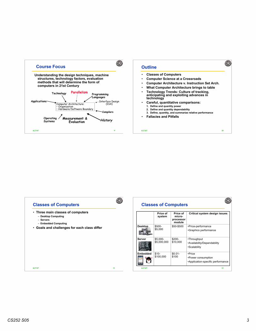
• Old Conventional Wisdom: Power is free, Transistors expensive• New Conventional Wisdom: “Power wall” Power expensive, Xtors free

(Can put more on chip than can afford to turn on)• Old CW: Sufficiently increasing Instruction Level Parallelism via

compilers, innovation (Out-of-order, speculation, VLIW, …)• New CW: “ILP wall” law of diminishing returns on more HW for ILP• Old CW: Multiplies are slow, Memory access is fast• New CW: “Memory wall” Memory slow, multiplies fast

(200 clock cycles to DRAM memory, 4 clocks for multiply)• Old CW: Uniprocessor performance 2X / 1.5 yrs• New CW: Power Wall + ILP Wall + Memory Wall = Brick Wall

– Uniprocessor performance now 2X / 5(?) yrs⇒ Sea change in chip design: multiple “cores”

(2X processors per chip / ~ 2 years)» More simpler processors are more power efficient

Crossroads: Conventional Wisdom in Comp. Arch

8/27/07 15

Crossroads: Uniprocessor Performance

• VAX : 25%/year 1978 to 1986• RISC + x86: 52%/year 1986 to 2002• RISC + x86: ≈20%/year 2002 to present

From Hennessy and Patterson, ComputerArchitecture: A Quantitative Approach, 4thedition, October, 2006 ≈20%/year

8/27/07 16

Sea Change in Chip Design• Intel 4004 (1971): 4-bit processor,

2312 transistors, 0.4 MHz,10 micron PMOS, 11 mm2 chip

• Processor is the new transistor?

• RISC II (1983): 32-bit, 5 stagepipeline, 40,760 transistors, 3 MHz,3 micron NMOS, 60 mm2 chip

• 125 mm2 chip, 0.065 micron CMOS= 2312 RISC II+FPU+Icache+Dcache

– RISC II shrinks to ~ 0.02 mm2 at 65 nm– Caches via DRAM or 1 transistor SRAM (www.t-ram.com) ?– Proximity Communication via capacitive coupling at > 1 TB/s ?

(Ivan Sutherland @ Sun / Berkeley)

CS252 S05 5

8/27/07 17

Déjà vu all over again?

• Multiprocessors imminent in 1970s, ‘80s, ‘90s, …• “… today’s processors … are nearing an impasse as

technologies approach the speed of light..”David Mitchell, The Transputer: The Time Is Now (1989)

• Transputer was premature⇒ Custom multiprocessors strove to lead uniprocessors⇒ Procrastination rewarded: 2X seq. perf. / 1.5 years

• “We are dedicating all of our future product development tomulticore designs. … This is a sea change in computing”

Paul Otellini, President, Intel (2004)• Difference is all microprocessor companies switch to

multiprocessors (AMD, Intel, IBM, Sun; all new Apples 2 CPUs)⇒ Procrastination penalized: 2X sequential perf. / 5 yrs⇒ Biggest programming challenge: 1 to 2 CPUs

8/27/07 18

Problems with Sea Change

• Algorithms, Programming Languages, Compilers,Operating Systems, Architectures, Libraries, … notready to supply Thread Level Parallelism or DataLevel Parallelism for 1000 CPUs / chip,

• Architectures not ready for 1000 CPUs / chip• Unlike Instruction Level Parallelism, cannot be solved by just by

computer architects and compiler writers alone, but also cannotbe solved without participation of computer architects

• Computer Architecture: A Quantitative Approach)explores shift from Instruction Level Parallelism toThread Level Parallelism / Data Level Parallelism

8/27/07 19





8/27/07 20

Instruction Set Architecture: Critical Interface

instruction set

software

hardware

• Properties of a good abstraction– Lasts through many generations (portability)– Used in many different ways (generality)– Provides convenient functionality to higher levels– Permits an efficient implementation at lower levels

CS252 S05 6

8/27/07 21

Example: MIPS0r0

r1°°°r31PClohi

Programmable storage2^32 x bytes31 x 32-bit GPRs (R0=0)32 x 32-bit FP regs (paired DP)HI, LO, PC

Data types ?Format ?Addressing Modes?

Arithmetic logicalAdd, AddU, Sub, SubU, And, Or, Xor, Nor, SLT, SLTU,AddI, AddIU, SLTI, SLTIU, AndI, OrI, XorI, LUISLL, SRL, SRA, SLLV, SRLV, SRAV

Memory AccessLB, LBU, LH, LHU, LW, LWL,LWRSB, SH, SW, SWL, SWR

ControlJ, JAL, JR, JALRBEq, BNE, BLEZ,BGTZ,BLTZ,BGEZ,BLTZAL,BGEZAL

32-bit instructions on word boundary

8/27/07 22

Instruction Set Architecture“... the attributes of a [computing] system as seen bythe programmer, i.e. the conceptual structure andfunctional behavior, as distinct from the organizationof the data flows and controls the logic design, andthe physical implementation.”

– Amdahl, Blaauw, and Brooks, 1964SOFTWARESOFTWARE

-- Organization of Programmable Storage

-- Data Types & Data Structures: Encodings & Representations

-- Instruction Formats

-- Instruction (or Operation Code) Set

-- Modes of Addressing and Accessing Data Items and Instructions

-- Exceptional Conditions

8/27/07 23

ISA vs. Computer Architecture• Old definition of computer architecture

= instruction set design– Other aspects of computer design called implementation– Insinuates implementation is uninteresting or less challenging

• Our view is computer architecture >> ISA• Architect’s job much more than instruction set

design; technical hurdles today more challengingthan those in instruction set design

• Since instruction set design not where action is,some conclude computer architecture (using olddefinition) is not where action is

– Disagree on conclusion– Agree that ISA not where action is (ISA in CA:AQA 4/e appendix)

8/27/07 24

Comp. Arch. is an Integrated Approach

• What really matters is the functioning of the completesystem

– hardware, runtime system, compiler, operating system, andapplication

– In networking, this is called the “End to End argument”

• Computer architecture is not just about transistors,individual instructions, or particular implementations

CS252 S05 7

8/27/07 25

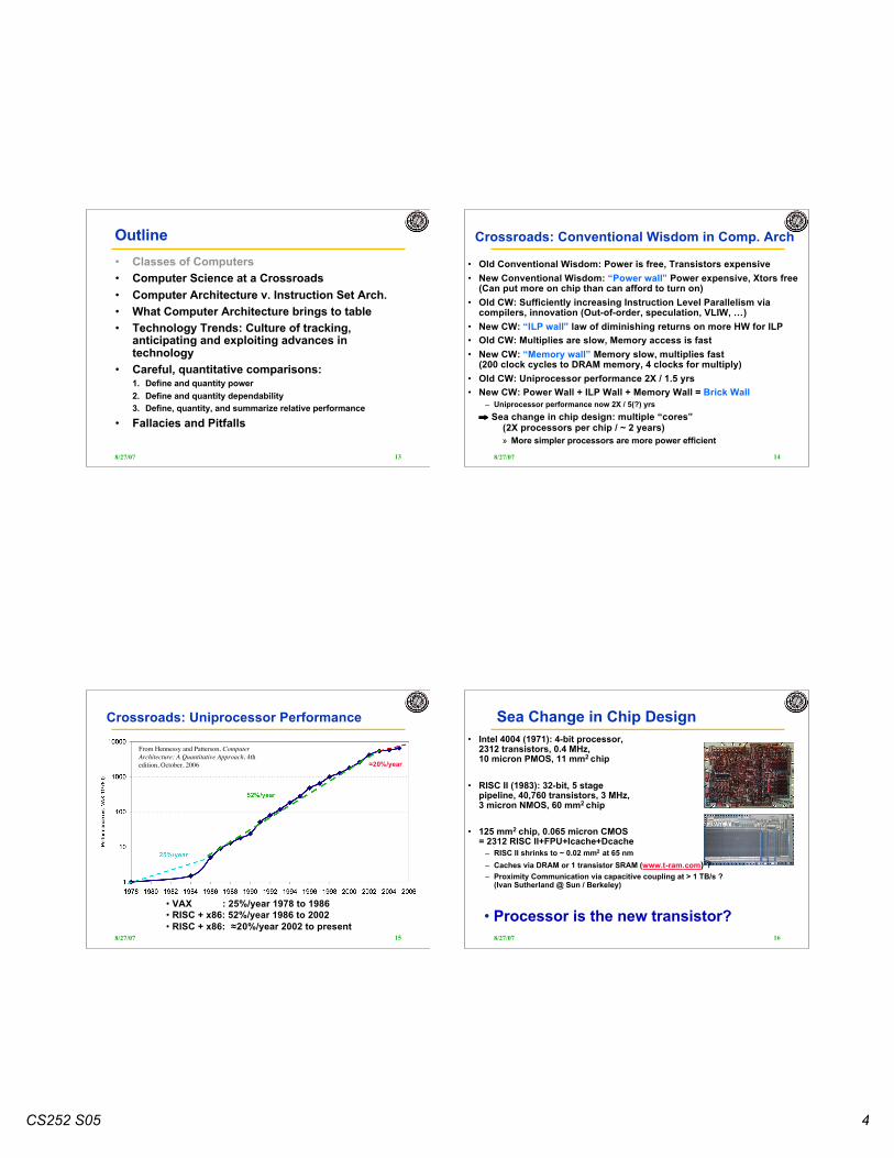
Computer Architecture isDesign and Analysis

Design

Ana lys is

Architecture is an iterative process:• Searching the space of possible designs• At all levels of computer systems

Creativity

Good IdeasGood IdeasMediocre IdeasBad Ideas

Cost /PerformanceAnalysis

8/27/07 26

Outline• Classes of Computers Computer Science at a

Crossroads• Computer Architecture v. Instruction Set Arch.• What Computer Architecture brings to table• Technology Trends: Culture of tracking,




8/27/07 27

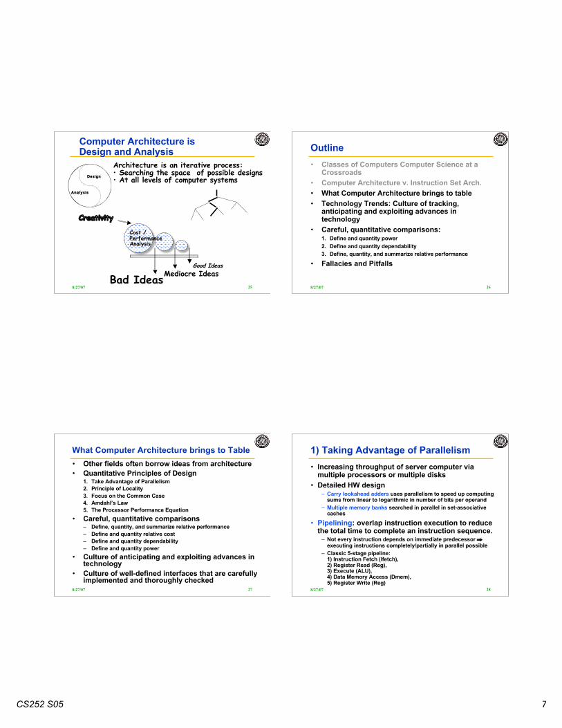
What Computer Architecture brings to Table• Other fields often borrow ideas from architecture• Quantitative Principles of Design

1. Take Advantage of Parallelism2. Principle of Locality3. Focus on the Common Case4. Amdahl’s Law5. The Processor Performance Equation

• Careful, quantitative comparisons– Define, quantity, and summarize relative performance– Define and quantity relative cost– Define and quantity dependability– Define and quantity power

• Culture of anticipating and exploiting advances intechnology

• Culture of well-defined interfaces that are carefullyimplemented and thoroughly checked

8/27/07 28

1) Taking Advantage of Parallelism• Increasing throughput of server computer via

multiple processors or multiple disks• Detailed HW design

– Carry lookahead adders uses parallelism to speed up computingsums from linear to logarithmic in number of bits per operand

– Multiple memory banks searched in parallel in set-associativecaches

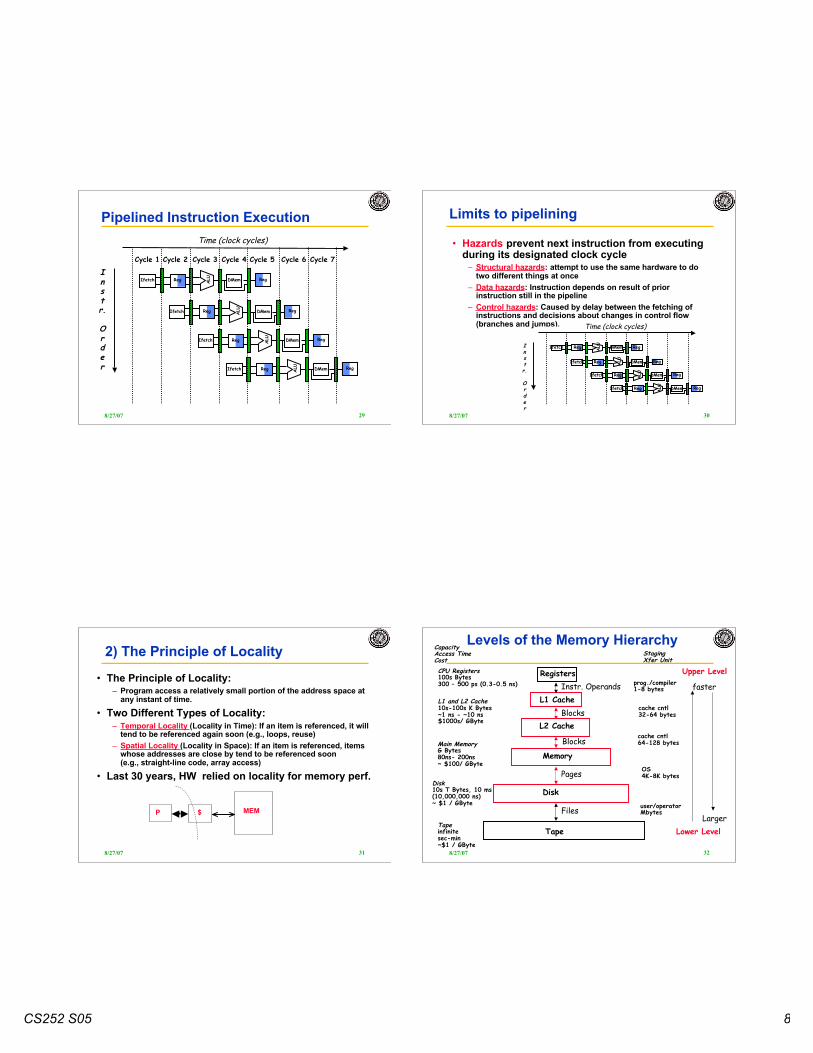
• Pipelining: overlap instruction execution to reducethe total time to complete an instruction sequence.

– Not every instruction depends on immediate predecessor ⇒executing instructions completely/partially in parallel possible

– Classic 5-stage pipeline:1) Instruction Fetch (Ifetch),2) Register Read (Reg),3) Execute (ALU),4) Data Memory Access (Dmem),5) Register Write (Reg)

CS252 S05 8

8/27/07 29

Pipelined Instruction Execution

Instr.

Order

Time (clock cycles)

Reg ALU DMemIfetch Reg




Cycle 1 Cycle 2 Cycle 3 Cycle 4 Cycle 6 Cycle 7Cycle 5

8/27/07 30

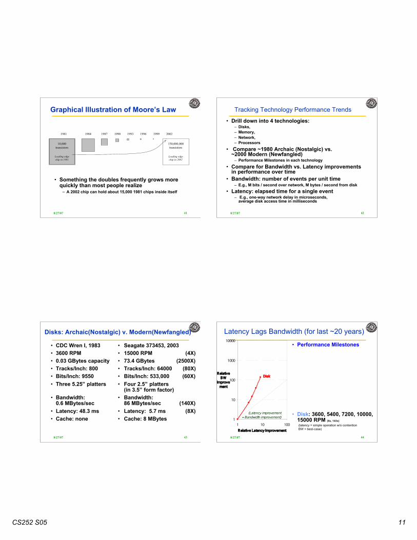
Limits to pipelining

• Hazards prevent next instruction from executingduring its designated clock cycle

– Structural hazards: attempt to use the same hardware to dotwo different things at once

– Data hazards: Instruction depends on result of priorinstruction still in the pipeline

– Control hazards: Caused by delay between the fetching ofinstructions and decisions about changes in control flow(branches and jumps).

Instr.

Order

Time (clock cycles)





8/27/07 31

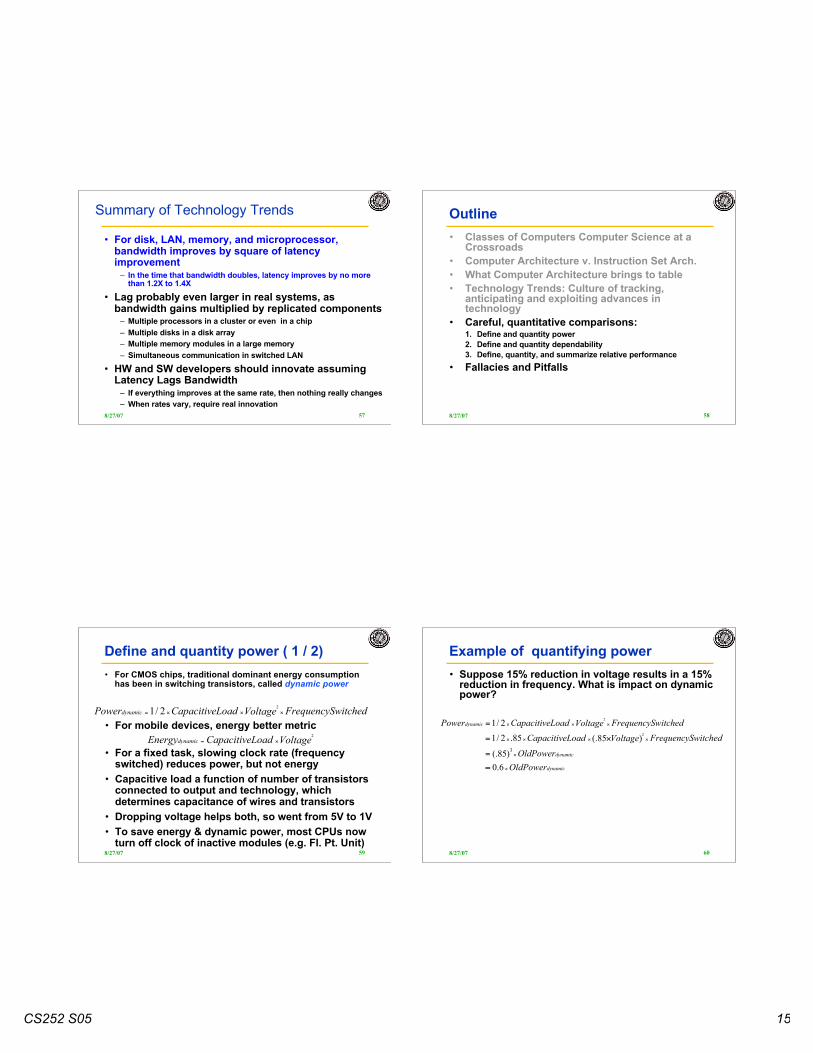
2) The Principle of Locality

• The Principle of Locality:– Program access a relatively small portion of the address space at

any instant of time.

• Two Different Types of Locality:– Temporal Locality (Locality in Time): If an item is referenced, it will

tend to be referenced again soon (e.g., loops, reuse)– Spatial Locality (Locality in Space): If an item is referenced, items

whose addresses are close by tend to be referenced soon(e.g., straight-line code, array access)

• Last 30 years, HW relied on locality for memory perf.

P MEM$

8/27/07 32

Levels of the Memory Hierarchy

CPU Registers100s Bytes300 – 500 ps (0.3-0.5 ns)

L1 and L2 Cache10s-100s K Bytes~1 ns - ~10 ns$1000s/ GByte

Main MemoryG Bytes80ns- 200ns~ $100/ GByte

Disk10s T Bytes, 10 ms (10,000,000 ns)~ $1 / GByte

CapacityAccess TimeCost

Tapeinfinitesec-min~$1 / GByte

Registers

L1 Cache

Memory

Disk

Tape

Instr. Operands

Blocks

Pages

Files

StagingXfer Unit

prog./compiler1-8 bytes

cache cntl32-64 bytes

OS4K-8K bytes

user/operatorMbytes

Upper Level

Lower Level

faster

Larger

L2 Cachecache cntl64-128 bytesBlocks

CS252 S05 9

8/27/07 33

3) Focus on the Common Case• Common sense guides computer design

– Since its engineering, common sense is valuable• In making a design trade-off, favor the frequent

case over the infrequent case– E.g., Instruction fetch and decode unit used more frequently

than multiplier, so optimize it 1st– E.g., If database server has 50 disks / processor, storage

dependability dominates system dependability, so optimize it 1st• Frequent case is often simpler and can be done

faster than the infrequent case– E.g., overflow is rare when adding 2 numbers, so improve

performance by optimizing more common case of no overflow– May slow down overflow, but overall performance improved by

optimizing for the normal case• What is frequent case and how much performance

improved by making case faster => Amdahl’s Law

8/27/07 34

4) Amdahl’s Law

( )enhanced

enhancedenhanced

new

oldoverall

Speedup

Fraction Fraction

1

ExTime

ExTime Speedup

+!

==

1

Best you could ever hope to do:

( )enhancedmaximum Fraction - 1

1 Speedup =

( ) !"

#$%

&+'(=

enhanced

enhancedenhancedoldnew Speedup

FractionFraction ExTime ExTime 1

8/27/07 35

Amdahl’s Law example• New CPU 10X faster• I/O bound server, so 60% time waiting for I/O

( )

( )56.1

64.0

1

10

0.4 0.4 1

1

Speedup

Fraction Fraction 1

1 Speedup

enhanced

enhancedenhanced

overall

==

+!

=

+!

=

• Apparently, its human nature to be attracted by 10Xfaster, vs. keeping in perspective its just 1.6X faster

8/27/07 36

5) Processor performance equation

CPU time = Seconds = Instructions x Cycles x Seconds Program Program Instruction Cycle

Inst Count CPI Clock RateProgram X

Compiler X (X)

Inst. Set. X X

Organization X X

Technology X

inst count

CPI

Cycle time

CS252 S05 10

8/27/07 37

What’s a Clock Cycle?

• Old days: 10 levels of gates• Today: determined by numerous time-of-flight

issues + gate delays– clock propagation, wire lengths, drivers

Latchor

register

combinationallogic

8/27/07 38






8/27/07 39

Trends in IC Technology• The most important trend in embedded systems -

Moore’s Law– Predicted in 1965 by Intel co-founder Gordon Moore– IC transistor capacity has doubled roughly every 18 months

for the past several decades

10,000

1,000

100

10

1

0.1

0.01

0.001

Logic transistorsper chip

(in millions)

1981

1983

1985

1987

1989

1991

1993

1995

1997

1999

2001

2003

2005

2007

2009

8/27/07 40

Moore’s Law• Wow

– This growth rate is hard to imagine, most peopleunderestimate

– How many ancestors do you have from 20 generations ago» I.e. roughly how many people alive in the 1500’s did it take

to make you» 220 = more than 1 million people

– This underestimation is the key to pyramid schemes!

CS252 S05 11

8/27/07 41

Graphical Illustration of Moore’s Law

• Something the doubles frequently grows morequickly than most people realize

– A 2002 chip can hold about 15,000 1981 chips inside itself

1981 1984 1987 1990 1993 1996 1999 2002

Leading edgechip in 1981

10,000transistors

Leading edgechip in 2002

150,000,000transistors

8/27/07 42

Tracking Technology Performance Trends

• Drill down into 4 technologies:– Disks,– Memory,– Network,– Processors

• Compare ~1980 Archaic (Nostalgic) vs.~2000 Modern (Newfangled)

– Performance Milestones in each technology• Compare for Bandwidth vs. Latency improvements

in performance over time• Bandwidth: number of events per unit time

– E.g., M bits / second over network, M bytes / second from disk• Latency: elapsed time for a single event

– E.g., one-way network delay in microseconds,average disk access time in milliseconds

8/27/07 43

Disks: Archaic(Nostalgic) v. Modern(Newfangled)

• Seagate 373453, 2003• 15000 RPM (4X)• 73.4 GBytes (2500X)• Tracks/Inch: 64000 (80X)• Bits/Inch: 533,000 (60X)• Four 2.5” platters

(in 3.5” form factor)• Bandwidth:

86 MBytes/sec (140X)• Latency: 5.7 ms (8X)• Cache: 8 MBytes

• CDC Wren I, 1983• 3600 RPM• 0.03 GBytes capacity• Tracks/Inch: 800• Bits/Inch: 9550• Three 5.25” platters

• Bandwidth:0.6 MBytes/sec

• Latency: 48.3 ms• Cache: none

8/27/07 44

Latency Lags Bandwidth (for last ~20 years)

• Performance Milestones

• Disk: 3600, 5400, 7200, 10000,15000 RPM (8x, 143x)

(latency = simple operation w/o contentionBW = best-case)

1

10

100

1000

10000

1 10 100

Relative Latency Improvement

Relative

BW

Improve

ment

Disk

(Latency improvement = Bandwidth improvement)

CS252 S05 12

8/27/07 45

Memory: Archaic (Nostalgic) v. Modern (Newfangled)

• 1980 DRAM(asynchronous)

• 0.06 Mbits/chip• 64,000 xtors, 35 mm2

• 16-bit data bus permodule, 16 pins/chip

• 13 Mbytes/sec• Latency: 225 ns• (no block transfer)

• 2000 Double Data Rate Synchr.(clocked) DRAM

• 256.00 Mbits/chip (4000X)• 256,000,000 xtors, 204 mm2

• 64-bit data bus perDIMM, 66 pins/chip (4X)

• 1600 Mbytes/sec (120X)• Latency: 52 ns (4X)• Block transfers (page mode)

8/27/07 46

Latency Lags Bandwidth (last ~20 years)• Performance Milestones

• Memory Module: 16bit plainDRAM, Page Mode DRAM, 32b,64b, SDRAM,DDR SDRAM (4x,120x)

• Disk: 3600, 5400, 7200, 10000,15000 RPM (8x, 143x)


1

10

100

1000

10000

1 10 100


Relative

BW

Improve

ment

MemoryDisk


8/27/07 47

LANs: Archaic (Nostalgic)v. Modern (Newfangled)

• Ethernet 802.3• Year of Standard: 1978• 10 Mbits/s

link speed• Latency: 3000 µsec• Shared media• Coaxial cable

• Ethernet 802.3ae• Year of Standard: 2003• 10,000 Mbits/s (1000X)

link speed• Latency: 190 µsec (15X)• Switched media• Category 5 copper wire

Coaxial Cable:

Copper coreInsulator

Braided outer conductorPlastic Covering

Copper, 1mm thick, twisted to avoid antenna effect

Twisted Pair:"Cat 5" is 4 twisted pairs in bundle

8/27/07 48

Latency Lags Bandwidth (last ~20 years)

• Performance Milestones

• Ethernet: 10Mb, 100Mb,1000Mb, 10000 Mb/s (16x,1000x)


• Disk: 3600, 5400, 7200, 10000,15000 RPM (8x, 143x)


1

10

100

1000

10000

1 10 100


Relative

BW

Improve

ment

Memory

Network

Disk


CS252 S05 13

8/27/07 49

CPUs: Archaic (Nostalgic) v. Modern (Newfangled)

• 1982 Intel 80286• 12.5 MHz• 2 MIPS (peak)• Latency 320 ns• 134,000 xtors, 47 mm2

• 16-bit data bus, 68 pins• Microcode interpreter,

separate FPU chip• (no caches)

• 2001 Intel Pentium 4• 1500 MHz (120X)• 4500 MIPS (peak) (2250X)• Latency 15 ns (20X)• 42,000,000 xtors, 217 mm2

• 64-bit data bus, 423 pins• 3-way superscalar,

Dynamic translate to RISC,Superpipelined (22 stage),Out-of-Order execution

• On-chip 8KB Data caches,96KB Instr. Trace cache,256KB L2 cache

8/27/07 50

Latency Lags Bandwidth (last ~20 years)

• Performance Milestones• Processor: ‘286, ‘386, ‘486,

Pentium, Pentium Pro,Pentium 4 (21x,2250x)

• Ethernet: 10Mb, 100Mb,1000Mb, 10000 Mb/s (16x,1000x)


• Disk : 3600, 5400, 7200, 10000,15000 RPM (8x, 143x)

1

10

100

1000

10000

1 10 100


Relative

BW

Improve

ment

Processor

Memory

Network

Disk


CPU high,Memory low(“MemoryWall”)

8/27/07 51

Rule of Thumb for Latency Lagging BW

• In the time that bandwidth doubles, latencyimproves by no more than a factor of 1.2 to 1.4

(and capacity improves faster than bandwidth)

• Stated alternatively:Bandwidth improves by more than the squareof the improvement in Latency

8/27/07 52

Computers in the News• “Intel loses market share in own backyard,”

By Tom Krazit, CNET News.com, 1/18/2006• “Intel's share of the U.S. retail PC market fell by

11 percentage points, from 64.4 percent in thefourth quarter of 2004 to 53.3 percent. … CurrentAnalysis' market share numbers measure U.S.retail sales only, and therefore exclude figuresfrom Dell, which uses its Web site to sell directlyto consumers. …AMD chips were found in 52.5 percent of desktopPCs sold in U.S. retail stores during that period.”

• Technical advantages of AMD Opteron/Athlon vs.Intel Pentium 4 as we’ll see in this course.

CS252 S05 14

8/27/07 53

6 Reasons Latency Lags Bandwidth

1. Moore’s Law helps BW more than latency• Faster transistors, more transistors,

more pins help Bandwidth» MPU Transistors: 0.130 vs. 42 M xtors (300X)» DRAM Transistors: 0.064 vs. 256 M xtors (4000X)» MPU Pins: 68 vs. 423 pins (6X)» DRAM Pins: 16 vs. 66 pins (4X)

• Smaller, faster transistors but communicateover (relatively) longer lines: limits latency

» Feature size: 1.5 to 3 vs. 0.18 micron (8X,17X)» MPU Die Size: 35 vs. 204 mm2 (ratio sqrt ⇒ 2X)» DRAM Die Size: 47 vs. 217 mm2 (ratio sqrt ⇒ 2X)

8/27/07 54

6 Reasons Latency Lags Bandwidth (cont’d)

2. Distance limits latency• Size of DRAM block ⇒ long bit and word lines

⇒ most of DRAM access time• Speed of light and computers on network• 1. & 2. explains linear latency vs. square BW?

3. Bandwidth easier to sell (“bigger=better”)• E.g., 10 Gbits/s Ethernet (“10 Gig”) vs.

10 µsec latency Ethernet• 4400 MB/s DIMM (“PC4400”) vs. 50 ns latency• Even if just marketing, customers now trained• Since bandwidth sells, more resources thrown at bandwidth,

which further tips the balance

8/27/07 55

4. Latency helps BW, but not vice versa• Spinning disk faster improves both bandwidth and

rotational latency» 3600 RPM ⇒ 15000 RPM = 4.2X» Average rotational latency: 8.3 ms ⇒ 2.0 ms» Things being equal, also helps BW by 4.2X

• Lower DRAM latency ⇒More access/second (higher bandwidth)

• Higher linear density helps disk BW (and capacity), but not disk Latency

» 9,550 BPI ⇒ 533,000 BPI ⇒ 60X in BW


8/27/07 56

5. Bandwidth hurts latency• Queues help Bandwidth, hurt Latency (Queuing Theory)• Adding chips to widen a memory module increases

Bandwidth but higher fan-out on address lines mayincrease Latency

6. Operating System overhead hurtsLatency more than Bandwidth

• Long messages amortize overhead;overhead bigger part of short messages


CS252 S05 15

8/27/07 57

Summary of Technology Trends

• For disk, LAN, memory, and microprocessor,bandwidth improves by square of latencyimprovement

– In the time that bandwidth doubles, latency improves by no morethan 1.2X to 1.4X

• Lag probably even larger in real systems, asbandwidth gains multiplied by replicated components

– Multiple processors in a cluster or even in a chip– Multiple disks in a disk array– Multiple memory modules in a large memory– Simultaneous communication in switched LAN

• HW and SW developers should innovate assumingLatency Lags Bandwidth

– If everything improves at the same rate, then nothing really changes– When rates vary, require real innovation

8/27/07 58






8/27/07 59

Define and quantity power ( 1 / 2)• For CMOS chips, traditional dominant energy consumption

has been in switching transistors, called dynamic power

witchedFrequencySVoltageLoadCapacitivePowerdynamic !!!=2

2/1

• For mobile devices, energy better metricVoltageLoadCapacitiveEnergydynamic

2

!=

• For a fixed task, slowing clock rate (frequencyswitched) reduces power, but not energy

• Capacitive load a function of number of transistorsconnected to output and technology, whichdetermines capacitance of wires and transistors

• Dropping voltage helps both, so went from 5V to 1V• To save energy & dynamic power, most CPUs now

turn off clock of inactive modules (e.g. Fl. Pt. Unit)8/27/07 60

Example of quantifying power• Suppose 15% reduction in voltage results in a 15%

reduction in frequency. What is impact on dynamicpower?

dynamic

dynamic

dynamic

OldPower

OldPower

witchedFrequencySVoltageLoadCapacitive

witchedFrequencySVoltageLoadCapacitivePower

!

!

!!!!

!!!

"

=

!=

=

6.0

)85(.

)85(.85.2/1

2/1

3

2

2

CS252 S05 16

8/27/07 61

Define and quantity power (2 / 2)• Because leakage current flows even when a

transistor is off, now static power important too

• Leakage current increases in processors withsmaller transistor sizes

• Increasing the number of transistors increasespower even if they are turned off

• In 2006, goal for leakage is 25% of total powerconsumption; high performance designs at 40%

• Very low power systems even gate voltage toinactive modules to control loss due to leakage

VoltageCurrentPower staticstatic !=

8/27/07 62






8/27/07 63

Define and quantity dependability (1/3)• How decide when a system is operating properly?• Infrastructure providers now offer Service Level

Agreements (SLA) to guarantee that theirnetworking or power service would be dependable

• Systems alternate between 2 states of servicewith respect to an SLA:

1. Service accomplishment, where the service isdelivered as specified in SLA

2. Service interruption, where the delivered serviceis different from the SLA

• Failure = transition from state 1 to state 2• Restoration = transition from state 2 to state 1

8/27/07 64

Define and quantity dependability (2/3)• Module reliability = measure of continuous service

accomplishment (or time to failure). 2 metrics

1. Mean Time To Failure (MTTF) measures Reliability2. Failures In Time (FIT) = 1/MTTF, the rate of failures

• Traditionally reported as failures per billion hours of operation

• Mean Time To Repair (MTTR) measures ServiceInterruption– Mean Time Between Failures (MTBF) = MTTF+MTTR

• Module availability measures service as alternatebetween the 2 states of accomplishment andinterruption (number between 0 and 1, e.g. 0.9)

• Module availability = MTTF / ( MTTF + MTTR)

CS252 S05 17

8/27/07 65

Example calculating reliability• If modules have exponentially distributed

lifetimes (age of module does not affectprobability of failure), overall failure rate is thesum of failure rates of the modules

• Calculate FIT and MTTF for 10 disks (1M hourMTTF per disk), 1 disk controller (0.5M hourMTTF), and 1 power supply (0.2M hour MTTF):

=

=

MTTF

eFailureRat

8/27/07 66

Example calculating reliability• If modules have exponentially distributed

lifetimes (age of module does not affectprobability of failure), overall failure rate is thesum of failure rates of the modules

• Calculate FIT and MTTF for 10 disks (1M hourMTTF per disk), 1 disk controller (0.5M hourMTTF), and 1 power supply (0.2M hour MTTF):

hours

MTTF

FIT

eFailureRat

000,59

000,17/000,000,000,1

000,17

000,000,1/17

000,000,1/5210

000,200/1000,500/1)000,000,1/1(10

!

=

=

=

++=

++"=

8/27/07 67






8/27/07 68

Performance(X) Execution_time(Y)n = =

Performance(Y) Execution_time(X)

Definition: Performance• Performance is in units of things per sec

– bigger is better

• If we are primarily concerned with response time

performance(x) = 1 execution_time(x)

" X is n times faster than Y" means

CS252 S05 18

8/27/07 69

Performance: What to measure• Usually rely on benchmarks vs. real workloads• To increase predictability, collections of benchmark

applications, called benchmark suites, are popular• SPECCPU: popular desktop benchmark suite

– CPU only, split between integer and floating point programs– SPECint2000 has 12 integer, SPECfp2000 has 14 integer pgms– SPECCPU2006 to be announced Spring 2006– SPECSFS (NFS file server) and SPECWeb (WebServer) added as

server benchmarks

• Transaction Processing Council measures serverperformance and cost-performance for databases

– TPC-C Complex query for Online Transaction Processing– TPC-H models ad hoc decision support– TPC-W a transactional web benchmark– TPC-App application server and web services benchmark

8/27/07 70

How Summarize Suite Performance (1/5)

• Arithmetic average of execution time of all pgms?– But they vary by 4X in speed, so some would be more important

than others in arithmetic average

• Could add a weights per program, but how pickweight?

– Different companies want different weights for their products

• SPECRatio: Normalize execution times to referencecomputer, yielding a ratio proportional toperformance =

time on reference computertime on computer being rated

8/27/07 71


• If program SPECRatio on Computer A is 1.25 timesbigger than Computer B, then

B

A

A

B

B

reference

A

reference

B

A

ePerformanc

ePerformanc

imeExecutionT

imeExecutionT

imeExecutionT

imeExecutionT

imeExecutionT

imeExecutionT

SPECRatio

SPECRatio

==

==25.1

• Note that when comparing 2 computers as a ratio,execution times on the reference computer dropout, so choice of reference computer is irrelevant

8/27/07 72


• Since ratios, proper mean is geometric mean(SPECRatio unitless, so arithmetic mean meaningless)

n

n

i

iSPECRatioeanGeometricM !

=

=1

1. Geometric mean of the ratios is the same as theratio of the geometric means

2. Ratio of geometric means= Geometric mean of performance ratios⇒ choice of reference computer is irrelevant!

• These two points make geometric mean of ratiosattractive to summarize performance

CS252 S05 19

8/27/07 73


• Does a single mean well summarize performance ofprograms in benchmark suite?

• Can decide if mean a good predictor by characterizingvariability of distribution using standard deviation

• Like geometric mean, geometric standard deviation ismultiplicative rather than arithmetic

• Can simply take the logarithm of SPECRatios, computethe standard mean and standard deviation, and thentake the exponent to convert back:

( )

( )( )( )i

n

i

i

SPECRatioStDevtDevGeometricS

SPECRation

eanGeometricM

lnexp

ln1

exp1

=

!"

#$%

&'= (

=

8/27/07 74


• Standard deviation is more informative if knowdistribution has a standard form

– bell-shaped normal distribution, whose data are symmetricaround mean

– lognormal distribution, where logarithms of data--not dataitself--are normally distributed (symmetric) on a logarithmicscale

• For a lognormal distribution, we expect that68% of samples fall in range95% of samples fall in range• Note: Excel provides functions EXP(), LN(), and

STDEV() that make calculating geometric meanand multiplicative standard deviation easy

[ ]gstdevmeangstdevmean !,/

[ ]22,/ gstdevmeangstdevmean !

8/27/07 75






8/27/07 76

Fallacies and Pitfalls (1/2)• Fallacies - commonly held misconceptions

– When discussing a fallacy, we try to give a counterexample.• Pitfalls - easily made mistakes.

– Often generalizations of principles true in limited context– Show Fallacies and Pitfalls to help you avoid these errors

• Fallacy: Benchmarks remain valid indefinitely– Once a benchmark becomes popular, tremendous

pressure to improve performance by targetedoptimizations or by aggressive interpretation of therules for running the benchmark:“benchmarksmanship.”

– 70 benchmarks from the 5 SPEC releases. 70% weredropped from the next release since no longer useful

• Pitfall: A single point of failure– Rule of thumb for fault tolerant systems: make

sure that every component was redundant sothat no single component failure could bringdown the whole system (e.g, power supply)

CS252 S05 20

8/27/07 77

Fallacies and Pitfalls (2/2)• Fallacy - Rated MTTF of disks is 1,200,000 hours or

≈ 140 years, so disks practically never fail• But disk lifetime is 5 years ⇒ replace a disk every 5

years; on average, 28 replacements wouldn't fail• A better unit: % that fail (1.2M MTTF = 833 FIT)• Fail over lifetime: if had 1000 disks for 5 years

= 1000*(5*365*24)*833 /109 = 36,485,000 / 106 = 37= 3.7% (37/1000) fail over 5 yr lifetime (1.2M hr MTTF)

• But this is under pristine conditions– little vibration, narrow temperature range ⇒ no power failures

• Real world: 3% to 6% of SCSI drives fail per year– 3400 - 6800 FIT or 150,000 - 300,000 hour MTTF [Gray & van Ingen 05]

• 3% to 7% of ATA drives fail per year– 3400 - 8000 FIT or 125,000 - 300,000 hour MTTF [Gray & van Ingen 05]

Documents

EEL 5764 Introduction - ann.ece.ufl.edu · Introduction Ch 1 - Fundamentals of Computer Design ... Midterms-40% –2 midterms »One ... •ISS for your own custom assembly language