AD-A1uG 385 COLD RE61ONS RESEARCH AND ENGINEERING LAS HANOVER NH F/e 13/1EVALUATING THE HEAT PUMP ALTERNATIVE FOR HEATING ENCLOSED WASTE--ETC(U)NAT 82 C J MARTEL. B E PHETTEPLACE

UNCLASSIFIED CRREL-SR-82-10 NLEEEEEEEEEEEEllE/hE/h/hEEE/hEIIELL

Special Report 82-10 /May 1982US Army Corps

May 1982EngineeCold Regions Research &Engineering Laboratory

Evaluating the heat pump alternative forheating enclosed wastewater treatmentfacilities in cold regions

C.J. Martel and Gary E. Phetteplace

-1--!,

JIUL 2 1982WJ

A

Propered forOFFICE OF THE CHIEF OF ENGINEERSAppro.d for public release, distributon unlmted. 82 07 02 18

UnclassifiedSECURITY CLASSIFICATION OF THIS PAGE (W.n Dat Fnf.,.d)

REPORT DOCUMENTATION PAGE BEFORE COMPLETING FORM

I. REPORT NUMBER 2 GOVT ACCESSION NO. 3 RECIPIENT'S CATALOG NUMBER

Special Report 82-10 1 , .!: - '

4TITLE (anld Subtitle) 5 TYPE OF REPORT 8, PERIOD COVERED

EVALUATING; THlE HEAT PUMP ALTERNATIVE FOR

HEATING ENCLOSED WASTEWATER TREATMENT FACI~IITIES

IN COLD REGIONS 6 PERFORMING ORG. REPORT NUMBER

7. AUTHOR(.) S. CONTRACT OR GRANT NUMBER(-)

C. 3ames Martel and Gary E. Phetteplace

9. PERFORMING ORGANIZATION NAME AND ADDRESS 10. PROGRAM ELEMENT. PROJECT. TASKAREA A WORK UNIT NUMBERS

U.S. Army Cold Regions Research and DPrect 4A762730AT42,Engineering Laboratory

DA o r t

Hanover, New Hampshire 03755 Task C, Work Unit C01

I. CONTROLLING OFFICE NAME AND ADDRESS 12. REPORT DATE

Office of the Chief of Engineers MayWashington, D.C. 20314 13. NUMBER OF PAGES

29

14. MONITORING AGENCY NAME & ADDRESS(I1 dllferent from Controlln4 Offil c e ) 15. SECURITY CLASS. (of this report)

Unclassified15.. DECLASSIFICATION,'DOWNGRADING

SCHEDULE

16. DISTRIBUTION STATEMENT (of this Report)

Approved for public release; distribution unlimited.

17. DISTRIBUTION STATEMENT (of the abstract eritered In Block 20, If different from Report)

IS. SUPPLEMENTARY NOTES

19. KEY WORDS (Continue on reverse aide If necessary wnd Identlfy by block number)

Cold regionsHeat pumpsHeat recoveryWaste treatment

20. ABSTRACT ('tllR,,, eve sie' f st i eo d Idenrwify by block number)

-This report presents a five-step procedure for evaluating the technical andeconomic feasibility of using heat pumps to recover heat from treatment planteffluent. The procedure is meant to be used at the facility planning levelby engineers who are unfamiliar with this technology. An example of the useof the procedure and general design information are provided. Also, the re-port reviews the operational experience with heat pumps at wastewater plantslocated in Fairbanks, Alaska, Madison, Wisconsin, and Wilton, Maine. .

' /!

D IJAN 75 3 EOITIION OF I NOV 65 IS OBSOLETE UcasfeS T Unclassified i ~SECURITV CLASSIFICATION OF THISI PAGE (Wlhken Del. Entered)

*'i *

PREFACE

This report was prepared by C. James Martel, Environmental Engineer,

of the Civil Engineering Research Branch, and Gary E. Phetteplace,

Mechanical Engineer, of the Applied Research Branch, Experimental

Engineering Division, U.S. Army Cold Regions Research nd Engineering

Laboratory. Funding for this research was provided by'DA Project

4A762730AT42, Design, Construction and Operations Technology for Cold

Regions, Task C, Cold Regions Base Support: Maintenance and Operations,

Work Unit 001, Operations and Maintenance of Cold Regions Sanitary

Engineering Facilities.

Sherwood Reed and Dr. Virgil Lunardini of CRREL technically reviewed

the manuscript of this report.

-i

.I i

aria

CONTENTS

Aostract . .I

Preface............................Introduction ............................Theory of operation......................Coefficient of performance (COP) ..................Sizing the heat pump and estimating costs .............

Building heat load................... .Estimation of COP.................. . . . ... .. .. . ...Effluent flow rate to heat pump.............. . . .. . . .....

Estimation of cost and energy savins .. ......... 12ex l.............................13Step 1. Determine the heating load ............. 13Step 2. Determine the capacity of the heat pump .. ..... 14Step 3. Determine the COP. ................ 15Step 4. Determine the evaporator tiou, rat . .. ....... 15Step 5. Estimate costs and energy savings .. ....... 15

Literature cited ........................ 19Appendix A: Degree-days and winter design temperatures for

large U.S. cities ................. 21

ILLUSTRATIONS

Figure1. Wastewater treatment plant in Wilton, Maine. .. ..... 22. iHeat pump unit and the Delafield-71artland plant. . . . 33. The principal components of a water-source heat pump 44. Approximate COP values for given effluent and heating

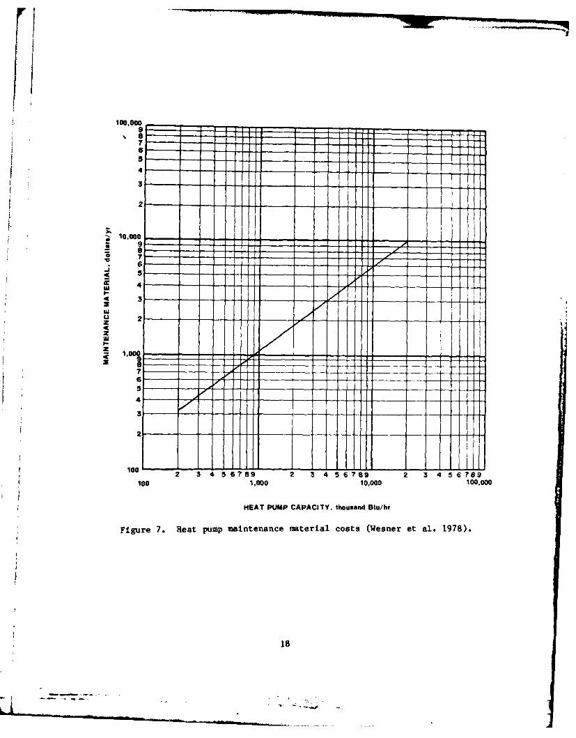
system temperatures .................. 75. Heat pump construction cost. .............. 166. Heat pump O&M labor requirements ............. 177. Heat pump maintenance material costs. ......... 18

TA.BLES

Table1. Typical hourly heat losses for three types of build-

ings.........................92. MNonthly average temperature of raw sewage .. ....... 113. Average heating value of some fuels .. ......... 124. Surmmary of heating requirements for hypothetical treat-

ment facility in Minneapolis, Minnesota .. ......145. Estimated costs of heat pump units ............ 166. Comparison of energy costs ................ 19

CONVERSION FACTORS: U.S. CUSTOMARY TO METRIC (SI) UNITSOF MEASUREMENT

These conversion factors include all the significant digitsgiven in the conversion tables in the ASTM Metric PracticeGuide (E 380), which has been approved for use by the De-partment of Defense. Converted values should be roundedto have the same precision as the original (see E 380).

Multiply By To obtain

inch 25.4* millimeter

foot 2 0.09290304* meter 2

foot 3 0.02831685 meter 3

gallon 3.785412* liter

pound/foot 3 16.01846 kilogram/meter 3

ton 907.1847 kilogramBtu 1055.056 joule

Btu/Ib *F 4186.800 joule/kilogram kelvin

degrees Fahrenheit toF = (toc- 32 )/1. 8 degrees Celsius

*Exact.

iv

EVALUATING THE HEAT PUMP ALTERNATIVE F'OR HEATING ENCLOSED

WASTEWJATER TREATMENT FACILITIES IN COLD REGIONS

by

C. James Martel and Gary Phetteplace

INTRODUCTION

Was tewater treatment facilities located in cold regions are often

enclosed to facilitate operation and maintenance. Because of today's high

cost of energy, heating these large enclosures with a conventional oil- or

gas-fired boiler can be expensive. A potentially less costly method is

to use a heat pump. This device extracts heat from the treatment plant

effluent and reuses it for space heating. Usually there is enough heat

energy in the effluent to supply the entire heating requirements of the

facility, including office and laboratory areas. A heat pump is especially

attractive in cold regions where the wastewater is kept warm in insulated

pipelines and heated utilidors. Also, the water supply is often heated in

order to avoid freezing in the distribution system. An added environmental

benef it of installing a heat pump is the reduction of thermal discharges to

the receiving stream.

The purpose of this report is to present a simple procedure that can

be used to evaluate the technical and economic feasibility of installing a

heat pump at new or existing wastewater treatment facilities. The intended

users of this procedure are environmental engineers, who generally are not

familiar with this technology. Information used to develop this procedure

was obtained from site visits, technical reports and papers, and heating!/Iventilation and air conditioning (HVAC) manuals. It should be noted that

this procedure is intended for feasibility studies at the facility planning

level only. The actual unit specifications should be determined by a

qualified HVAC specialist.

EXISTING HEAT PUMP INSTALLATIONS

One of the first sewage treatment plants to include a heat pump in its

initial design is located in Fairbanks, Alaska. This plant, completed in

the summer of 1976, has an average design flow of 8.0 million gallons per

Figure 1. Wastewater treatment plant in Wilton, Maine.

day (mgd) and an average wastewater temperature of 45'F. The wastewater

treatment processes include an aerated grit chamber, several pure-oxygen-

activated sludge units and a chlorine contact chamber. Approximately 12.5%

of the chlorinated effluent is diverted through two heat transfer coils and

a heat pump. The heat transfer coils supply the base heat load of the

facility while the heat pump is used as a booster unit when more heat is

needed. The heat transfer coils and heat pump are designed to heat and

ventilate a 38,880-ft 2 enclosure at 40*F when the outside air temperature

is as low as -60*F (Crews 1977). The total estimated heat load, including

ventilation, is 3.728 x 109 Btu/yr. The maximum rate of heat loss through

the enclosure was calculated to be 743,400 Btu/hr and the ventilation

requirement is 10,000 ft3/min. A backup heating system, consisting of

electrical resistance coils, is provided for supplemental heating.

The Wiltou, Maine, Wastewater Treatment Plant (Fig. 1), also success-

fully uses a heat pump to heat their enclosed treatment area. This

0.45-mgd plant was constructed using the latest energy-saving technologies,

including a heat pump, active and passive solar heating systems, digester

gas recovery and air-to-air heat recovery (Wilke and Fuller 1976). A study

conducted by Wright-Pierce, Architects and Engineers (1980) indicated that

the heat pump unit provided 60% of the total facility heating require-

ments. The unit was designed for a total heat output of 320,000 Btu/hr at

2

Figure 2. Heat pump unit at the Delafield-Hartland plant.

an effluent flow rate through the heat pump of 60 gal./min. The initial

cost of this unit was $11,400 in 1978.

After initial problems with the control circuitry were solved, a heat

pump unit performed satisfactorily during its first year of operation atthe Delafield-Hartland plant near Madison, Wisconsin I . This new plant has

a design flow of 2.2 mgd, and the treatment scheme includes primary

sedimentation, rotating biological contactors and rapid sand filtration.

The total heating load of this facility was estimated to be 1.0 x 106

Btu/hr (Budde et al. 1979). The heat pump (Fig. 2) was designed to supply

120*F water to the hot water heating system rather than the conventional

180*F. Because of this lower temperature, the size of the building heating

elements had to be increased by approximately 20%. The hot water produced

by the heat pump is stored in a large tank which can also be heated by

stand-by electric immersion heaters.

Heat pumps have been used for many years at numerous commercial and

industrial installations, but their use with sewage effluent is a rela-

tively new application of this technology. Some problems have been re-

ported due to the solids content and corrosive nature of wastewater.

I R. Hyde, Superintendent, Delafield-Hartland Wastewater Treatment Plant,

pers. comm., 1981.

3

High Pressure t or Rad atorsR t r

Condenser

Electric Motor

Compressor'

Suction and discharge valves omitted for clarity

ExpansionValve

Low PressureVav

Evaporator 10 (D

eSewage4WP Effluent in

Sewage

Effluent out

Figure 3. The principal components of a water-source heat pump(Phetteplace 1979).

Recently, the Fairbanks plant had to shut down its heat pump unit because

of corrosion in the evaporator caused by chlorine and sulfides in the

effluent 2 (Miko 1981). At the Wilton plant, the operator reported that he

had to frequently clean the effluent strainers which are located in the

supply line to the evaporator3 . He indicated that this problem could have

been avoided by installing larger strainers.

The heat pump unit in each of these plants is supplied with wastewater

of secondary effluent quality or better. A higher strength wastewater is

not used because of possible solids accumulattom and fouling problems on

the interior surface of the tubes in the evaporator unit of the heat pump

(see Fig. 3). Even with secondary effluent, a fine-screening device is

sometimes placed in the effluent supply line to trap solids escaping from

the clarifier.

The preferred location for the intake to the evaporator supply line is

just upstream of the overflow weir in the chlorine contact chamber. As

noted by Budde et al. (1979), this location is preferred because the

2 j. Miko, Superintendent, Fairbanks Municipal Wastewater Treatment Plant,

ers. comm., 1981.J. Thornton, Superintendent, Wilton, Maine, Wastewater Treatment Plant,

pers. comm., 1981.

4

chlorine should help to maintain clean evaporator tubes. However, chlorine

residual concentration should be carefully controlled in order to prevent

corrosion. The return line should be located downstream of the chlorine

contact chamber just before the effluent metering device. This location

avoids the potential adverse effects of low temperature return water on

disinfection.

THEORY OF OPERATION

A heat pump is a cyclic device that transfers heat from a lower temp-

erature source (e.g. the effluent) to a higher temperature sink (e.g. the

hot water heating systm). The most common example of a heat pump is a

refrigerator. It removes heat from the 1 '.q temperature of its interior and

rejects that heat to the higher !temperature on its exterior. Thus, it

1.pumps" heat back into its surroundings, where the heat originated. A heat

pump allows heat from a low temperature source such as treatment plant

effluent to be used at a higher temperature, such as is required for space

heating. The price paid for recovery of this waste heat is the cost of the

electrical energy used by the compressor.

With the aid of Figure 3 it is possible to trace the thermodynamic

cycle of a heat pump. Since this is a cyclic device, there is no true

starting or finishing point for the cycle; arbitrarily, the cycle will be

assumed to begin where the refrigerant is mostly liquid and at low tempera-

ture and pressure. This is the state of the refrigerant after it leaves

the expansion valve as shown in Figure 3 (state 1). The refrigerant then

enters the evaporator where it takes on sufficient heat from the effluent

to be evaporated from the liquid to the gaseous state at nearly constant

temperature and pressure (state 2). Next, the refrigerant enters the com-

pressor where the pressure is increased, a process that also increases the

temperature of the refrigerant (state 3). Finally, the gaseous refrigerant

flows into the condenser where heat is given up to the hot water heating

system. This heat is the latent heat of vaporization of the refrigerant as

it condenses from a gas to a liquid (state 4). The liquid refrigerant now

enters the expansion valve and has its pressure reduced. Upon exit from

the expansion valve, the refrigerant is now ready again to repeat the cycle

just described. The advantage of this cycle is that most of the heat input

occurs in the evaporator. This energy does not have an economic cost,

although some electrical energy is needed to run the compressor.

5

COEFFICIENT OF PERFORMANCE (COP)

The ratio of energy delivered to the building heating system vs the

energy required by the compressor is a measure of the efficiency of the

heat pump. This ratio, called the coefficient of performance (COP), is the

most important factor in determining the economic advantage of installing a

heat pump. A COP higher than 1.0 indicates that the energy output by the

heat pump is greater than the energy input so that an energy savings would

be realized. However, the operation and maintenance cost of the heat pump

must also be recovered. Typically, COP's of heat pumps used in wastewater

treatment plants range from 2.5 to 4.5.

The COP depends mainly on the temperature difference between the heat

source (wastewater effluent) and the heat delivery system, which in most

cases will be a hot water heating system. The greater the temperature dif-

ference, the lower the COP. For this reason it is desirable to use the

highest temperature heat source and the lowest practical delivery tempera-

ture. The relationship between effluent temperature, delivered tempera-

tures and COP is shown in Figure 4. This figure assumes a temperature drop

of 5'F across the evaporator, an approach temperature of 150F (temperature

difference between the effluent, or hot water, and refrigerant as they

approach the heat exchangers), and a combined motor/compressor efficiency

of 65%. Although these factors could vary for each heat pump installation,

they should be accurate enough for estimation purposes.

To maintain a high COP it is better to provide a greater flow through

the evaporator and drop the temperature of the effluent only a few

degrees than to provide a low flow and a large temperature drop. Usually,

the increased COP compensates for the higher pumnping costs. The allowable

temperature drop will depend on the minimum temperature of the effluent

during the winter. In the case of an existing plant, the minimum effluent

temperature can be determined from past data. For new plants the minimum

temperature must be estimated.

Another way to improve the COP is to design the hot water heating

system for temperatures in the 120'~ to 140*F range rather than th: standard

180*F. As mentioned previously, the COP improves as the temperature dif-

ference between the effluent and the hot water heating system decreases.

The cost of the larger radiators needed for a 1200 to 140*F heating systemIis small compared to the reduced operational cost at the higher COP (Niess1981). A heat pump can also be used at an existing plant equipped witha

6

E610 CP

iE

100•I-0

U,/

60 -- 15 F Approach Temperature-65% Efficiency

40 50 60 70 80 90Effluent Temperature (*F)

Figure 4. Approximate COP values for given ef-fluent and heating system temperatures.

standard heating system. However, supplemental heating may be required on

occasion. This supplemental heat could be supplied by the old boiler.

The heat pump system controls should be designed to automatically

lower the hot water supply temperature as the outdoor temperature in-

creases. This can be achieved with a control device which senses the temp-

erature of the return water from the heating system. As the temperature of

the return water increases, the control system reduces the compressor

energy input and causes the temperature of the supply water to decrease so

that the heat pump system operates at near the optimum COP.

Another way to increase the COP is to reduce on-off cycling by closely

matching the capacity of the heat pump with the load requirement. One

effective method of load control is through the use of a multi-speed or

variable speed compressor. This type of compressor reduces the energy

input by idling one or more cylinders as the load decreases. The improved

efficiency easily compensates for the additional cost of the special con-

trols.

7

SIZING THE HEAT PUMP AND ESTIMATING COSTS

Building Heat Load

The most important step in sizing a heat pump is to estimate the

building heat load. The heating load results from basic conduction losses

through walls, windows, ceiling and floor. Also air infiltration and

ventilation cause sizable heat losses, especially in enclosed sewage treat-

ment facilities where air exchange is necessary to control odors. These

losses vary from structure to structure depending on type and quality of

construction, ventilation requirements, and climatic conditions. The

heating load will also depend on the desired internal temperature of the

building. At cold regions facilities, the administration and laboratory

areas are usually maintained at 68'F while the enclosed treatment area may

be maintained at only 40 to 45*F.

Conduction heat losses per 1000 ft 2 of floor area can be calculated as

follows:

E = 24 HD (I)c

where Ec = annual building conduction losses, Btu/1000 ft2 of floor

area

H = hourly heat loss, Btu/1000 ft2 -hr-OF

D = degree days, *F day/yr.

The hourly heat loss value (H) can be estimated from the building construc-

tion criteria in Table 1. Degree day (D) information for 650, 550 and 45*F

base temperature can be obtained from Appendix A or local sources such as a

heating oil distributors. The designer should use the base temperature

closest to the desired internal temperature of the building.

Determining the total heating load will also require calculation of

the amount of infiltration and ventilation. Infiltration is the uncon-

trolled leakage of air into a building through cracks in the walls and

ceilings, and around doors and windows (including the result of opening and

closing doorways). Ventilation is the intentional movement of air into and

out of a building through specific openings. In general it is more energy

efficient to produce air exchange by installing a ventilation system, which

can be controlled, than by relying on infiltration, which cannot be con-

trolled.

Table 1. Typical'hourly heat loss for three types of buildings (Wesneret al. 1978).

Hourly heatType Construction loss (H), Btu/1000 ft2-hr-*F

A Uninsulated 820

B 3.5-in. wall insulation, 6.0-in. 450ceiling insulation, storm windows

C Same insulation as Type B, double 325glazed windows, floor insulation

The energy required to heat the infiltration and ventilation air, per

1000 ft2 of floor area, can be calculated as follows:

E - 466 haD (2)V

where Ev = annual ventilation heat losses, Btu/1000 ft2-yr

h = height of ceiling, ft

a = number of air changes/hr.

The constant 466 includes the specific heat of air (0.24 Btu/Ib-0 F), the

density of air (0.0809 lb/ft 3), the unit area of the building (1000 ft2 )

and the number of hours per day, Accepted values of "a" for both adminis-

trative and enclosed treatment areas range between four to six air changes

per hour (Wesner et al. 1978). The term D is degree days as defined in eq

1.

The combined annual heating loss for each 1000 ft2 is the sum of Ec

and Ev . This sum, when multiplied by the heated floor area of the

facility (expressed in 1000 ft2 ), will give the total heating load of the

facility. This is a conservative estimate because no credit is taken for

heat produced by internal sources such as lights and machinery. Solar heat

gain during the day is also not taken as a credit because the heating

equipment should be sized to meet the most adverse conditions, which

generally occur at night.

Heat Pump Capacity

Once the building heating load is calculated, the required heat pump

capacity (Q, in Btu/hr) can be determined by dividing the total annual

heating load by the number of hours per year of equivalent full load opera-

tion. The yearly hours of equivalent full load operation (N), i.e. the

r9

hours of use resulting if the total heating load for the year were supplied

at full capacity, can be calculated from climatic information as follows:

24 DN - B -T(3

where B is the base temperature of degree days (D) used in heat load

calculations C0F), and T the winter design temperature (0F).

The winter design temperature T is based on a probability distribution

of average hourly temperatures during the months of December, January and

February. This temperature can be found in the ASHRAE Cooling and Heating

Load Calculation Manual (1979) for many U.S., Canadian and foreign cities.

Appendix A lists winter design temperatures for a few selected cities in

the United States.

Since winter design temperatures were selected at the 97 1/2% and 99%

levels, there could be 54 and 22 hours, respectively, during an average

winter when the outdoor temperature is below the winter design tempera-

ture. During this period, the heat pump would be inadequate to supply the

heating load and freezing problems might occur, especially if the internal

design temperature of the building is already near freezing, as in the case

of an enclosed treatment area. Typically this area is only heated to 400

to 45*F. Therefore, for enclosed treatment areas it would be safer to use

the winter design temperature at the 99% level. The winter design tempera-

ture at the 97-1/2% level could be used for other areas where the internal

design temperature will be higher, say 68*F, and the risk of freezing is

smaller.

Estimation of COP

As mentioned earler, the COP can be estimated from Figure 4, but the

average effluent temperature during the winter must first be determined.

For existing plants this is not a problem since the effluent temperatures

can be measured directly. For new plants, however, the temperature must be

estimated from data obtained at other northern facilities. Data from eight

such facilities are shown in Table 2 for the months of October through

March. The average effluent temperature for these facilities during this

time period was approximately 50*F. Although these temperatures are for

raw sewage, they should not be significantly different from effluent temp-

eratures if the facility is enclosed. In evaluating the temperature drop

through an enclosed pure-oxygen-activated sludge system, Boyle (1976) con-

Table 2. Monthly average temperature ( 0 F) of raw sewage (Alter 1969).

Place Oct. Nov. Dec. Jan. Feb. Mar.

Aurora, 111. 49 49 50 48 47 46Canton, Ohio 56 50 47 42 40 42Flint, Mich. 63 58 53 50 48 45Schenectady, N.Y. 64 60 56 48 43 36Traverse City, Mich. 60 55 52 48 46 49Fairbanks, Alaska 53 52 52 52 51 51Juneau, Alaska 46 46 44 38 36 37Wilton, Me.* 62 57 50 46 44 43Average 57 53 51 47 44 43

*Temperature of secondary effluent (Wright-Pierce 1980)

cluded that the amount of heat loss was negligib-le and the temperature drop

through the system should not be greater than 1*F.

The data shown in Table 2 also indicate that effluent temperatures

will gradually decrease over the winter heating season. October usually

has the highest effluent temperatures and the March lowest. Thus, there is

a significant delay in the impact of cold ambient air on the temperature of

the sewage effluent. This delay is caused by the insulating effect of the

cover material above the collection system. An important benefit of this

delay is that higher effluent temperatures are available during the coldest

months of December and January. By the time the effluent temperature

reaches its lowest point in March the demand for heat has lessened con-

siderably.

Effluent Flow rate to Heat Pump

The effluent flow rate needed to supply the evaporator will depend on

the heat pump capacity, COP, and the temperature drop across the evapora-

tor. The heat pump capacity and COP car be determined as indicated

earlier. The temperature drop across the evaporator should only be 3* to

50F according to Niess (1981). Budde et al. (1979) report flow rates

ranging between 12 to 17% of the average wastewater flow. This percentage

will be higher for facilities where the entire treatment area is enclosed

and heated. Also, the percentage of effluent used by the heat pump will be

higher during the first few years because the initial flow will be lower

than the 20-year design value.

once the required heat pump capacity, COP, and temperature drop across

Table 3. Average heating value of some fuels.

Heating valueFuel (106gBtu)

#2 fuel oil, 1 US gallon 0.1385#4 fuel oil, I US gallon 0.145Natural gas, 1000 ft3 1.092Propane, 1000 ft3 2.560Bituminous steam coal, short ton 24.580Electricity, 1000 kilowatt hours 3.413

the evaporator are established, the volumetric flow rate can be calculated

as follows:

2000 Q (1 - 100

AT

where V - volumetric flow rate, gpm

Q - heat pump capacity, million Btu/hr

= compressor motor efficiency, %

AT - temperature drop across the evaporator, *F.

Since the motor efficiency is usually around 90%, eq 4 can be simpli-

fied to

2000 Q (1 -~- (5)

V AT(5

Estimation of Cost and Energy Savings

The construction, 0&M labor, and maintenance material costs as a func-

tion of heat pump capacity can be estimated from Figures 5, 6 and 7. These

costs are based on an Engineering News Record (ENR) Construction Cost Index

of 2499 (Jan. 1977).

The energy cost savings will depend on the cost of heating with an

alternative fuel source. The heating values of some alternative fuels are

shown in Table 3. The cost of these fuels will vary regionally and can be

determined by contacting local fuel suppliers. Boiler efficiency will also

affect the cost of an alternative heating systems. Oil- and coal-fired

boiler efficiences are usually about 70% while that of a gas-fired boiler

is about 807.. Electrical resistance heating is normally figured at 100%

efficiency. The heat pump efficiency is already included in the assump-

tions for determining the COP from Figure 4.

12

r! T rEXAMPLE

The following is an example of how to use the previous information to

properly size a heat pump unit and estimate energy savings. As mentioned

earlier, this procedure is meant for the feasibility planning stage only.

Nevertheless, this procedure should provide a relatively accurate estimate

of the energy savings, if any, resulting from a heat pump installation. A

competent HVAC specialist should be contacted for more detail in regard to

design specifications and cost information.

As part of a facility plan, the project engineer wishes to evaluate

the cost-effectiveness of installing a heat pump to supply the heating

needs for a 5-mgd plant located near Minneapolis, Minnesota. The total

floor area of this facility will be 27,000 ft2 of which 25,000 ft2 is for

an enclosed treatment area and the remaining 2000 ft2 is for the adminis-

trative and laboratory functions.

Step 1. Determine the heating load.

The building heat loss can be determined from eq 1. Type B construc-

tion is planned for the enclosed treatment area which results in an hourly

heat loss value (H) of 450 Btu/1000 ft2-hr-*F. This area will only be

heated to 40*F which should be sufficient to prevent freeze-ups and facili-

tate operator maintenance. With the 45*F base, the average degree day

reading for the Minneapolis area is 3309*F-day (see App. A). Type C con-

struction is proposed for the office area which has a H value of 325

Btu/1000 ft2-hr-OF. This area will be heated to the standard indoor design

temperature of 68*F. Therefore, the 65*F base will be used for this area

which results in an average degree day reading of 8382*F-day. From eq 1,

the building heat losses for the treatment and office areas are

Conduction heat loss for f2y= 24 x 450 x 3309 = 35.7 x 106 Btu/1000 ft2-yrenclosed treatment area

Conduction heat loss for= 24 x 325 x 8382 = 65.4 x 106 Btu/1000 ft 2 -yr.office area

The heating requirements due to ventilation can be calculated from

eq 2. The ceiling heights of the treatment and office areas will be 12 and

8 ft respectively. A ventilation requirement of four changes per hour was

assumed for both areas. From equation 2, the ventilation losses are

Ventilation heat loss, = 466 2 12 x 4 x 3309 - 74.0 x 106 Btu/1O00 ft2-yrenclosed treatment area

13

I - -I - -. . .. . . . I . . .I I . . . . II IIlll . . . . ..

Table 4. Summary of heating requirements for hypothetical treatment facility inMinneatpolis, Minnesota.

Conduction Ventilation heat Combined heat Area heatService loss, E loss, E loss, E + E loadC V C v

area (Btu/1000 ft2 -yr) (Btu/1000 ft 2-yr) (Btu/1000 ft2 -yr) (Btu/yr)

Enclosed 35.7 x 106 74.0 x 106 109.7 x 106 2472 x 106treatmentarea(25,000 ft 2 )

Offices 65.4 x 106 125.0 x 106 190.4 x 106 381 x 106

(2000 ft 2 )

Ventilation heat loss, = 466 x 8 x 4 x 8382 = 125.0 x 106 Btu/1000 ft 2-yroffice area

The combined heat losses can be determined by adding building and

ventilation heat losses for each area. To convert the combined heat losses

to a heat load, multiply the heat losses by the floor area expressed in

1000 ft2 . The total facility heat load is then the sum of each area heat

load. A summary of heat losses and heat loads in each area is shown in

Table 4. The total facility heat load is estimated to be 3123 x 106

Btu/yr.

Step 2. Determine the capacity of the heat pump.

The capacity or size of the heat pump can be determined by dividing

the heating load by the number of equivalent full load hours. From eq 3,

the number of equivalent full load hours (N) for the treatment and office

areas are 1302 and 2613 hours respectively. The winter design temperatures

(T) used in eq 3 were -16°F for the treatment area and -120 F for the office

area. For reasons discussed earlier, a lower winter design temperature

(-16 0 F) was used for the treatment area to allow a greater margin of

safety.

Since the heating requirements of the two areas are quite different,

separate heat pump units would be more efficient. Based on a heat load of

2742 x 106 Btu/yr (see Table 4) and 1302 equivalent full load hours, the

required capacity of unit 1, the heat pump unit for the enclosed treatment

area, is 2.1 x 106 Btu/hr (2742 x 106 Btu/yr + 1302 hr/yr). Likewise, the

required capacity of a smaller heat pump unit (unit 2) for the office area

is 0.15 x 106 Btu/hr.

14

Step 3. Determine the COP.

The COP can be estimated from Figure 4 once the effluent and hot water

heating system temperatures are established. Since this is a new plant, an

effluent temperature of 50'F will be assumed. The heating system tempera-

ture for unit I will be set at 90*F while unit 2 will be set at 120*F.

These temperatures should provide adequate heat transfer and allow each

heat pump to operate at a high COP. From Figure 4 the COP's are 4.1 and

2.8 for units I and 2 respectively.

Step 4. Determine the evaporator flow rate.

By assuming a 5*F drop across the evaporator, the flow rate can be

determined from eq 5.

Effluent flow rate through 4.001 . ( 657 gl/inevaporator of unit 1 5

Effluent flow rate through 2.008 .1 i 41 gal./minevaporator of unit 2 5

The total flow of effluent through both evaporators is then almost 700 gpm

at peak load, which is equi.valent to 1.0 ngd or approximately 20% of the

design flow.

Step 5. Estimate costs and energy savings.

The estimated construction 0&M labor and maintenance material costs

[or each heat pump unit were calculated from Figures 5, 6 and 7 for an

Engineering News-Record Construction Cost Index of 3610 (3 Sept 1981).

These costs (see Table 5) may be higher than for comparable oil- or gas-

fired systems; however, the energy saved by the heat pump should more than

conpensate. In a comparison of oil and heat pump heating systems, Budde et

al. (1979) determined that, although the heat pump system had higher

capital, 0&M labor, and maintenance material costs, the present worth cost

was lower because of the energy savings. As energy costs escalate, this

differential will undoubtedly increase. Also, for municipal treatmentplants, the initial cost of the heat pump could be offset by federal and

state grants.

The energy costs of heating with the heat pumps and various other

fuels are shown in Table 6. These costs were based on an annual heatingI

15

1.000.0009

6- -

100,000 I9

o 7i '

W= 6oI- 5 - - - : *0/

0 4___0U -4 - -'r : -

z 3___2I.-

z0zC. 10,000 - _ - -

S -- --

6--

1,000 4L § ~L2 3 4 5 6769 2 3 4 5 6 789 2 3 4 56789

100 1000 10.000 100.000

HEAT PUMP CAPACITY, thousand Stu/hr

Figure 5. Heat pump construction cost (Wesner et al. 1978).

Table 5. Estimated costs of heat pump units.

O&M labor and

Heat pump Service Capacity Construction* maintenance materiallarea (1000 Btu/hr) costs ($) costs ($/yr)

1 Enclosed 2100 86,676 4,400Treatment Area

2 Office area 150 13,000 530

• Based on ENR Construction Cost Index of 3610 (3 Sept. 1981).

t Includes labor costs @ $8/hr and maintenance material costs (see Fig. 6and 7).

16

10,000 __

75

4

3 ,

2

-II

8,

U

000

HET UM-APCIY touad tuh

3

for 2 eet iy $11/a.frfelol 9/o.o ca n 40/

prbal inces inteftrfferie otnet ie

I 1 .007 ' O I

10 L A2 3 4 5 6789 2 3 4 5 6 789 2 3 4 5 6789:100 1,000 10,000 100,000

HEAT PUMP CAPACITY, thousand Btu/hr

! Figure 6. Heat pump O&M labor requirements (Wesner et al. 1978).

i load of 3123 x 106 Btu and unit costs for the .Minneapolis area of O.04/kWh

: for electricity, $1.19/gal. for fuel oil, $97/ton for coal and $4.06/1000

ft 3 of natural gas . Also shown in Table 6 are the potential annual

i savings resulting from a heat pump installation vs other types of heating

~equipment. The minimum annual savings is $5,082 compared to an equivalentI gas boiler. The annual savings compared to a typical oil-fred boiler is

f $28,905. This cost differential in favor of a heat pump installation willl

probably increase in the future if fuel prices continue to rise.

A. Duval, St. Paul District, U.S. Army Corps of Engineers, St. Paul

Minnesota, pers. coum., 1981.

17

100,000

7

S10.000

Il

2

z 100 1001,0 0.0

1008

2 7 92 19 8

100~~~~ 1,0 1,0010.0

Table 6. Comparison of energy costs.

Annual* Extra energy cost comparedType of heating energy cost ($) to heat pump ($/yr)

Heat pumps 9,433

Elec. resistance 52,294 42,861

Oil-fired boiler 38,338 28,905

Coal fired boiler 17,608 8,175

Natural gas boiler 14,515 5,082

i Electrical resistance cost figures at 100% efficiency, oil- andcoal-fired boilers at 70% efficiency, and natural gas at 80% efficiency.The heat pump energy cost was calculated as follows:

2742x106 Btu/yr 381x106 Btu/yr $0.04/kWh4.1 + 2.8 3413 Btu/kWh = $9433.00

LITERATURE CITED

Alter, A.J. (1969) Sewerage and sewage disposal in cold regions. CRREL

Cold Regions Science and Engineering Monograph II-C5b.

American Society of Heating, Refrigerating and Air-Conditioning

Engineers, Inc. (1979) ASHRAE cooling and heating load calculation

manual. New York.

Boyle, J.D. (1976) Biological treatment process in cold climates. Water and

Sewage Works, p. 28-50.

Budde, P.E., M.D. Doran and W.R. Ratal (1979) Energy recovery from waste-

water treatment plant effluent. Journal of the Water Pollution

Control Federation, vol. 51, p. 2155.

Crews, P.B. (1977) Heating the Fairbanks, Alaska, wastewater treatment

facility with a heat-pump-treated effluent. Proceedings of an

International Symposium on Cold Regions Engineering, Univ. of Alaska,

Fairbanks.

Niess, R.C. (1981) Effluents and energy economics. Water/Engineering and

Management, August, 1981, p. 52-58.

Phetteplace G. (1979) Waste heat recovery for heating purposes. The

Northern Engineer, vol. 10, no. 3.

Strock, C. and R.L. Koral (1965) Handbook of Air Conditioning, Heating and

Ventilation. New York: Industrial Press, 2nd ed.

19

Wesner, G.M., G.L. Culp, T.S. Lineck and D.J. Hinrichs (1978) Energy con-

servation in municipal wastewater treatment. U.S. Environmental

Protection Agency Technical Report EPA-430/9-77-011.

Wilke, D.A. and D.R. Fuller (1976) Highly energy efficient Wilton Waste-

water Treatment Plant. Civil Engineering Magazine, May 1976, p.

70-72.

Wright-Pierce Architects/Engineers (1980) Integrated energy systems

monitoring municipal wastewater treatment plant, Wilton, Maine.

U.S. Environmental Protection Agency Intermediate Report, Contract

68-03-2587.

20

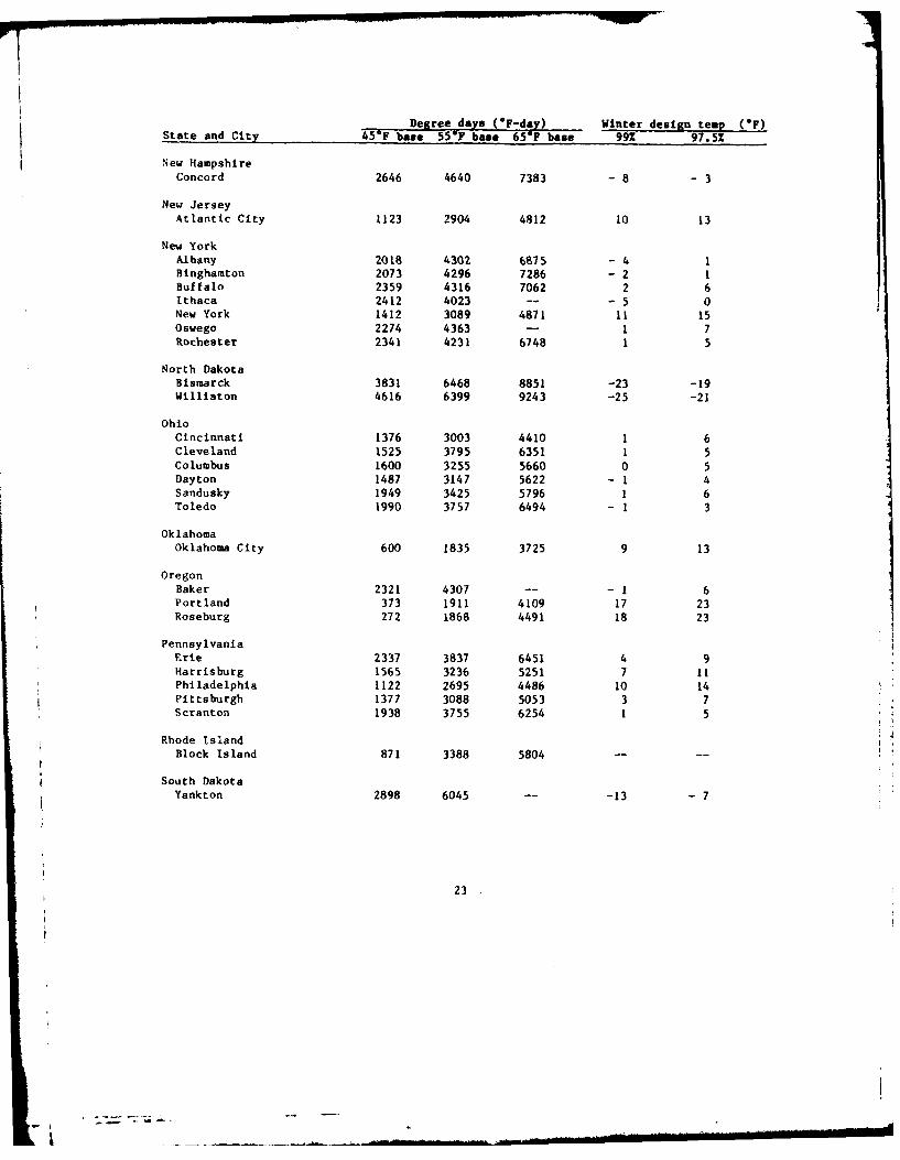
APPENDIX A. DEGREE-DAYS AND WINTER !ESIGN IEMPERAT'RES ]OR ;ELECTED L.S. UJTIL;

Degree days (F-day) 7 Winter design temp2

('F)

State and City 45°F baset

55'F base 65*Fase 99% 97.5%

AlaskaAnchorage 10864 -23 -18Fairbanks 14279 -51 -47

Juneau 9075 - 4 - INome 14171 -31 -27

ColoradoDenver 1548 3440 6283 - 5 1Grand Junc. 1757 3433 5641 2 7Pueblo 1499 3261 5462 - 7 0

Connecticut

Meriden -- 734 -- -- --

New Haven 1769 3237 5897 3 7

District of Columbia 1041 2487 4224 14 17

Idaho

Boise 1045 2814 5809 3 10

Lewiston 1034 2688 5542 - 1 6Pocatello 2161 4140 7033 - 8 - 1

IllinoisCairo 749 2119 3821 ....

Chicago 1969 3743 5882 - 3Springfield 1677 3289 5429 - 3 2

Indiana

Evansville 799 2335 4435 4 9Indianapolis 1397 2829 5699 - 2 2

Iowa

Davenport 2296 4142 -- -- --

Des Moines 2440 4180 6588 -10 - 5

Kansas

Dodge City 1385 2962 498b 0 5Topeka 1518 1811 5182 0 4Wichita 1152 2587 4620 3 7

Kentucky

Lexington -- 2557 4683 3 8

Louisville 1073 2294 4660 5 10

Strock and Koral (1956) Handbook of Air Cond., Heating and Ventilation, 2nd ed.2 ASHRAE (1979) Cooling and Heating Load Calculation Manual.

21

Degree days (*F-day) Winter design temp (°F)State and City 45*F base 55*F base 65°F base 99% 97.5%

Maineast Port 2956 5236 .-- --

Portland 2530 4572 7511 - 6 1

MarylandBaltimore 986 2491 4654 14 17

MassachusettsBoston 1787 3603 5634 6 9Nantucket 1514 3419 5891 -- --

MichiganAlpena 3131 5499 8506 -1] - 6Detroit 2240 4089 6232 3 6Escanaba 3699 5918 8481 -11 - 7Grand Haven 2405 3435 -- -- --

Grand Rapids 2332 4177 6894 1 5Houghton 4029 6112 -- -- --

Lansing 2537 4444 6909 - 3 1Sault Ste. Marie 4049 6575 9048 -12 - 8

MinnesotaDuluth 4419 6774 1000 -21 -16Minneapolis 3309 5417 8382 -16 -12Moorhead 4796 6572 -- -- --

St. Paul 2497 5497 -- -16 -12

MissouriKansas City 1463 2980 4711 2 6Saint Louis 1186 2745 4484 2 6Springfield 982 2423 4900 3 9

MontanaHavre 3736 5874 8182 -18 -11Helena 2843 5071 8129 -21 -16Kalispell 2874 5131 8191 -14 - 7

NebraskaLincoln 3023 3850 5864 - 5 - 2North Platte 2291 4152 6684 - 8 - 4

Omaha 2284 3982 6612 - 8 - 3

Valentine 2833 4801 7425 -- --

NevadaWinnemucca 1670 3468 6761 1 3

22

Degree days ('F-day) Winter design temp ('F)State and City 45F base 55'F base 65'F base 99% 97.5Z

I New HampshireConcord 2646 4640 7383 - 8 - 3

New JerseyAtlantic City 1123 2904 4812 10 13

New YorkAlbany 2018 4302 6875 - 4 1Binghamton 2073 4296 7286 - 2 1Buffalo 2359 4316 7062 2 6Ithaca 2412 4023 -- - 5 0New York 1412 3089 4871 11 15Oswego 2274 4363 - 1 7Rochester 2341 4231 6748 1 5

North DakotaBismarck 3831 6468 8851 -23 -19Williston 4616 6399 9243 -25 -21

OhioCincinnati 1376 3003 4410 1 6Cleveland 1525 3795 6351 1 5Columbus 1600 3255 5660 0 5Dayton 1487 3147 5622 - 1 4Sandusky 1949 3425 5796 1 6Toledo 1990 3757 6494 - 1 3

OklahomaOklahoma City 600 1835 3725 9 13

OregonBaker 2321 4307 -- - 1 6Portland 373 1911 4109 17 23Roseburg 272 1868 4491 18 23

PennsylvaniaErie 2337 3837 6451 4 9Harrisburg 1565 3236 5251 7 11Philadelphia 1122 2695 4486 10 14Pittsburgh 1377 3088 5053 3 7Scranton 1938 3755 6254 1 5

Rhode IslandBlock Island 871 3388 5804

South DakotaYankton 2898 6045 -- -13 7

23

Degree days (°F-day) Winter design temp (*F)State and City 45F base 55°F base 65°F base 99% 97.5%

TennesseeChattanooga 242 1398 3254 13 18Knoxville 431 1741 3494 13 19Memphis 166 1284 3015 13 18Nashville 419 1678 3578 9 14

UtahModena 1978 3981 -- -- --

Salt Lake City 1475 3202 6052 3 8

VermontBurlington 3014 4984 8269 -12 - 7

VirginiaLynchburg 554 1928 4166 12 16Norfolk 260 1496 3421 20 22Richmond 549 1895 3865 14 17

WashingtonNorth Head 184 2062 - -- --

Seattle 408 2185 4424 22 27Spokane 1741 3672 6655 - 6 2

West VirginiaElkins 1506 3327 5675 1 6Parkersburg 1147 2784 4754 7 11

WisconsinGreenbelt 3318 5331 8029 -13 - 9LaCrosse 3034 3992 7589 -13 - 9Madison 3067 4850 7863 -11 - 7Milwaukee 2657 4617 7635 - 8 - 4

WyomingCheyenne 2500 4700 7381 - 9 - ILander 3208 5450 7870 -16 -11

24

DATE

ILMEI