A WORLD VERTICAL NETWORK.(U)

FEB A0 0 L COLOMBO F1962-79-C-002?NLASSIFIED DGS-296 AFBL-TR-80-0077 NL

1 0

EEEEEEEE

III"11112 11111_LOjj2

111L 25 III 1 1IIII1.

CHROCOPY RESOLUT4 TEST CHARTNAHOtNAL HOLRIAtU Of STANDAR[P I 10€ A

'VIP

-4',

R 'w

;l . -, 0 *' VO,51A, n5

- WE!

SECURITY ;WNICATION or ris PAGE ("~eiOnR Detgatoeto

A~EFR COMPETIN VETALNEWOK

As. rp orREOR NT NUMPER oe

.~~~DeDept.n of Geodeti Scieno.e9

The Ohio State University - 1958 Neil Avenue 61102FColumbus, Ohio 43210 61" 2 1AW 17 G 1-

11. coNrO IN OFICE NAME AND AORESSAir Fore Geophysics Laboratory Fb watHanscornAFE, Massachusetts 01730 i FebaP,0"%9wContract Monitor: Bela Szabo/LW 63

14. MONITORING -AENCY NAME & AOORESS(If different from Controllind Office) 15. SECURITY CL.ASS. (of this report)TUnclassified13ai. DEC. ASSIPICATION/OOW0NGRAOING

14. OISTRIUIUTION STATEMENT (of thi ReCrt EGU

A -Approved for public release; distribution unlimited

17. OISTRIGUTION STATEMENT (0f CA*oberact entered In Stoak 20, It different frost Reort)

16I. SUPPLEMENTARY NOTES

It. KEY WORDS (Continue on Peverit id. It noeoowy aid Identify by block numethr)

geodesy, height, gravity, potential, geoid

2O. ANSTRA 1(Continue an reverao side It neceoesey aid Identify by block number)

Gravimetric data, levelling, and precise position fixes using artificial satel-ltes or the Mvoon could be combined to estimate the potential difference between

benchmarks situated far apart to an accuracy of a few tenths of kgal m. This issubstantially better than what can be obtained with tide gauges, which are affected bythe stationary sea surface topography. A set of these benchmarks can link nationaland continental levelling nets into a unifiled World Vertical Network.

OD ,~ 173 OITON F I OV 5 I OSOLEI tnc las 9if ledSECURITY CLASSIP CATION O T MIS PAGE (w hben Do t ered) -

Foreword

This report was prepared by Dr. Oscar L. Colombo, Post Doctoral Researcher,* Department of Geodetic Science, The Ohio State University, under Air Force

Contract No. F19,28-79-C-0027, The Ohio State University Research FoundationProject No. 711904, Project Supervisor Richard H. Rapp. The contract coveringthis research A administered by the Air Force Geophysics Laboratory, HaiscomAir Force Base, Massachusetts, with Mr. Bela Szabo, Contract Monitor.

Aveai

-iil.It

Specia

Acknowledgements

The author thanks professor Richard H. Rapp (O.S.U. Columbus) for his

help in clarifying and sorting out the basic ideas presented here; to Dr. Hans

Sihnkel (Graz) for revising most of the mathematical formulations, a very time-

consuming task he undertook most selflessly. To Reiner Rummel (Munich),

Christian Tscherning (Copenhagen) and Carl Wagner (formerly with NASA's

Goddard Space Flight Center and now living in Mountainview, California), many

thanks for their comments. The author is in debt to Kostas Katsambalos for

his careful proofreading of the text.

Pamela Pozderac is acknowledged for her typing of the manuscript, which

went through several revis ions.

.

Table of Contents

Foreword . iii

1. ntroduction .............................................. I

1.1. Definition of World Vertical Network .......................... 2

2. Method of Approach ............................. ................. 2

2. 1. Formulation of the Problem ................................ 3

2.2. Estimating T by Least Squares Collocation ................... 4

2.3. Data Arrangement ......................................... 8

2.4. Adjustment Theory ........................................ 9

3. Characteristics of the Data ...................................... 11

3.1. Position Fixes .............................. ............... 11

3. 2. Reference Model of the Gravity Field ......................... 12

3.3. Propagation of Position Errors through the Computed U ........ 14

3.4. Gravity Anomalies .......................................... 15

3.5. Propagation of Position Errors through Gravity Anomalies ...... 18

3.6. Levelling .................................................. 20

4. Computing Disturbing Potentials ................................... 21

4. 1. Reducing the Dimension of the Data Covariance Matrix .......... 21

4.2. Estimating T from 4 instead of 4g ........................ 24

4.3. Accuracies for T (P,) Estimated over 50 and 100 Caps ......... 26

4.4. Correlation Among Estimation Errors...................... 29

5. The Accuracy of the Adjusted Vertical Connection ................... 31

5. 1. Transoceanic Connections Using Several 50 Caps ............... 32

-v-

5.2. optimal Estimator for the Potential Difference Between Two Caps. 34

5.3. Height Differences Between inaccessible Points ................ 36

5.4. Some Questions Regarding Accuracy Estimates ................. 37

6. Conclusions .................................................. 3

References ...................................................... 4

AppendixA ...................................................... 4

Appendix B....................................................... 46

-vi-

1. Introduction

Since spirit levelling cannot be used across the oceans, connecting con-tinental vertical networks has long been a challenge for both oceanographers andgeodesists. Among the former, Cartwright (1963) calculated a tie between theBritish and the European nets across the English channel. Because the oceanog-raphic method requires a knowledge of currents that is not available for largerbodies of water, the geodesist Erik Tengstrom (1965) tried using gravimetry anddeflections of the vertical to compute a geoidal profile through the Eastern Medi-terranean, from Athens to Alexandria. His results suffered from lack of data.Lelgemann (1976) proposed unifying vertical datums by means of gravimetry,levelling, and very accurate position determinations, as those expected by theproponents of lunar laser ranging (Silverber et al., 1976). The late R. S.Mather (1978) considered the possibilities open for datum unification by constantimprovements in gravity field models (notably Goddard's GEM series) and thelarge amounts of information provided by the altimeter satellites whose proto-type has been GEOS-3.

Dynamic effects create a "sea surface topography", or departure of themean sea surface from a true equipotential. This topography is not very wellknown at present, and has an estimated r. m. s. value of about 1 m. Tidegauges determine the position of mean sea level at their locations, so the errormade by assuming that their mean sea level marks are on the same equipotentialsurface (geoid) is of the order of /'2 x (r. m. s. of the stationary sea surfacetopography) - 1.5 kgalm. Without any additional work, Nature provides a world"levelling net" of 1. 5 kgal m accuracy.

Would it be possible to obtain better transoceanic links using the variousforms of geodetic data that are available at present, or are likely to becomeavailable in the near future? Could it be feasible, with such data, to establishbenchmarks for levelling inside continents, rather like inland "tide gauges",whose potential differences are known so well that they can be used to constrainthe adjustment of the net to reduce distortion? If so, in a more distant future,similar benchmarks could be used to survey other components of the Solar System,where only the Earth has any significant amount of free surface water.

In this work the reader will not find more than a passing reference to the geoid,a notion that appears inseparable from that of vertical height and of vertical datum.Since the geoid has been regarded as the natural universal datum by geodesists, afew words of explanation are due. The reason for its omission here is that, howeveruseful otherwise, the geoid is not essential to the setting up of a vertical network,at least in theory. Such network, ultimately, is a set of potential differences es-timated among the points that form the net, in particular the primary points orbenchmarks. These potential differences do not convey information on the abso-lute potential of the gravity field, so they can be referred to any number of levelsurfaces, and not exclusively to one. For the same reason their meaning is not

-1-

>,- 'i~" - -- - -

dependent on which surface is selected, and it remains intact even if no surfaceis selected. The reason why the geoid is so ubiquitous in the literature onlevelling may be the complete reliance that levelling has had on tide gauges,idealized as points on the geoid. As long as gauges play a basic role, theconcept of reference surface is relevant to levelling.

Here, instead of heights above an equipotential surface, we are going toconsider distances to the center of mass of the Earth, or to a reference ellipsoidalcentered on this point. Such approach is not unreasonable today, when new po-sitioning techniques are being developed that promise accuracies far better thanthose available in the past. Methods based on the Global Positioning Systemsatellites, on Lageos, and on portable interferometric and lunar laser rangingstations, are expected to achieve near decimeter accuracy in relative position,over continental distances.

In recent years, the use of artificial satellites has changed many aspectsof geodesy. Space techniques for obtaining position fixes and models of thegravity field are in constant development, and both the quality and the quantityof the data provided by spacecraft are increasing. This work shall explorehow these advances may affect levelling. Next paragraph, to begin with, intro-duces a basic idea: a World Vertioal Network established without recourse toany reference surface, or geold. In a way, such network is the datum.

1.1. Definition of World Vertical Network

The World Vertical Network (WVN) is a set of estimated potential differencesamong benchmarks situated in various continents.

A network of potential differences can be translated immediately into a varietyof height systems such as those described by Krakiwsky and Mueller (1965). Po-tential differences are intrinsic to the set of benchmarks selected, and are indepen-dent on the choice of "geoid", or on the precise knowledge of the zero harmonicof the Earth's potential, present estimates of which have an uncertainty of some3 kgal m. Existing regional networks can be tied to the closest benchmarks tocreate a dense, unified global levelling net. Any benchmark potential can be usedto reference all points tied to the net. If so desired, the level surface throughthis arbitrary point may be regarded as a "geoid".

2. Method of Approach

If we had a perfect model of the gravity field and exact position fixes ingeocentric coordinates at two points on the Earth's surface, then we could usethis Information to find the potential of each point and, from this, their potentialdifference. Repeating this process for all possible pairs of points out of a givenset of benchmarks, the end result would be an exact WVN. Unfortunately, models

-2-

Ald .t. Asti.

and fixes are never perfect, so the potential differences must have some errors.To reduce these errors, we could combine the field model, which being finitecannot contain information above certain spatial frequencies, with additionaldata such as gravimetry, rich in high frequencies, particularly from the vicinityof the benchmarks.

2.1. Formulation of the Problem

If V is the gravitational potential due to the mass of the Earth and externalto its surface, and U is a reference potential defined by a spherical harmonic'smodel:

U(0,X,r) = - -[1 + E (a/r)"PF.(sino) Ct,.cosmX+Sk.sinrnXJ] (2.1)r 2

where: T3,, fully normalized Legendre function of the first kind, degree n andorder m ;

r,4,X geocentric distance, latitude, and longitude;G universal gravitational constant;M mass of the Earth;a mean equatorial radius of the Earth;

C., Sn* normalized spherical harmonic coefficients;N maximum degree and order for terms present in the model;

then the disturbing potential T at a point P of geocentric coordinates rp,0p,Xp is

T(P) = V(P) - U (P) (2.2)

The gravity potential of the Earth is

W(P) = V(P) + ((P) (2.3)

where o ( P) = w rp' cos 2 Op corresponds to the rotational potential, w being

the angular velocity of the planet about its spin axis. The potential difference be-tween two points such as P and Q is, therefore,

A W(P,Q) = U(P) + T(P) + 0 (P) - U(Q) - T(Q) - o(Q) (2.4)

With both P and Q on the Earth's surface, the uncertainties in the calculatedvalues of o(P) or o(Q), due to errors in the known positions of P and Q , will bethousands of times smaller than those arising in the determination of U (P), U (Q),

-3-

I

T (P) and T (Q). Consequently, only errors in the computed values in the right

hand side of

4 W (P, Q) V-P) [ O ] V(P) - (Q)

U(P) + T(P) - (U(Q) + T(Q)1 (2.5)

shall be Included in the error analysis that constitutes the major part of whatfollows.

2.2. Estimating T by Least Squares Collocation

The use of linear regression for predicting and filtering geodetic dataappears to have been first proposed by Kaula (1959). Further developed byMoritz and others, this approach has become a familiar technique that hasshown its value in many applications. Least squares collocation, as geodesistscall it, provides a way of combining all relevant data into estimates of unobservedvariables (minimum variance prediction), or into more reliable estimates ofthose actually observed (minimum variance filtering). For further information onthis method, see Moritz (1972).

If T is to be estimated at point P, then the linear, unbiased, minimumvariance estimator of T (P) is

T(P) = f_ d = f?(z+n) (2.6)

where

f = (Czz + D) - ' C'z (2.7)

is the optimal estimator vector, and

AT is the estimated disturbing potential, a scalar;

d = z + n is the N1 vector of measurements, or data vector;z is the N vector of signal component in the measurements;n is the N vector of the noise component in the measurements;

Ctz = M Tzr is the lxN covariance matrix (a row vector) of T and z;Czz = M z Z') is the N xl covariance matrix of the signal z;

D = M nn T ) is the N xN covariance matrix of the noise n.

The operator M f I represents some kind of average. D is supposed to bediagonal, because the noise is not correlated from measurement to measurement(white noise). Furthermore, these assumptions apply:

-4-

i;.p..

r

M z1= M - Mrd) = O (a null vector)and

M fz_nr , M T n' J are both null matrices.

More generally, we could be asked to obtain N. estimates (N vector ofestimates) from d, using an estimator matrix F such that

A.E = F' d (2.6)*

minimizes the mean square values of the components of the error vector

Ae - s - s

(s is the N, vector of true values of s). The variance-covariance matrix ofthese errors is

E = Mfee' = M(s- FTd)(s - Ftd) } = C,.-F C. 2z-C. 2 F+F r (Cgz+D)F (2.8)

where C, = M[ss 3 isa NxN. matrix, and Cz = Msz } is a N xNmatrix. Since the elements in the main diagonal of E are either positive orzero, minimizing each one of the mean square errors is the same as minimizingtheir sum, the trace of E (tr(E)). Accordingly (see for instance, (Rao, 1973)),

o r tr(E = _CT + (C~z + D) F = (a null matrix)or )

(C,,+D) F = CT (2.9)and, finally,

F = (C . + D)- Cd. (2.10)

Replacing (2.10) in (2.8) we get

E = C,. - Csz (Cz, + D)71 CT. (2. 11)

In the special case where s is the scalar T, we get (2. 7). The equations in thesystem (2.9) are known as "normal equations"; some people prefer to call them"Wiener-Hopf equations" because they bear a formal resemblance to the basicintegral equation of linear, invariant, minimum variance filtering in the time domain.

"5-

J*'5.

In geodetic applications, M I is an average on rotations of some sort.If all possible rotations about the origin (center of mass) are included, then thecovariance function ch of a function h of r,O and X

M(h(P) h(Q) f c h (P,Q) (2.12)

depends only on the spherical distance

Jpq = cos'[sin 0, sin + Cos 4 Cos q cos (4 - AQ)]

and on the geocentric distances rp and rQ. If both P and Q are on the samesphere ( rp = rQ ), then Chh depends on Op, alone. For this reason this type ofcovariance is known as isotropic, and the operator M( I is then called the iso-tropic average operator'. The elements of F depend on those of matrices C,and C,, and these elements are, in turn, values of the covariance functions

c,(p,Q) = Ms(P) z(Q)) and c..(P,Q) = Mtz(P) z(Q) .

A choice of Mt I determines those functions, their values, and, ultimately, theoptimal estimator matrix F. Rummel and Schwarz (1977) have discussed differenttypes of averages and covariance functions. From these considerations it is clearthat the optimal estimator is not unique, but it depends on what average we choose.The "easiest" choice is the isotropic average, because of the simplicity of thecorresponding covariance function. This function can be expanded as a series ofLegendre polynomials

c. (P,Q) = - (2n+l) (r a ., P.(CosWJ) (2.13).'10

where 65,,, , is the nth degree variance of the spherical harmonic coefficients ofu(O,X,r):

I'

6U =, + 9,..)(2n+ 1)1 (2.14)

The covariance between two functions u and v is

i There is a small problem with Mn nI, because the measurements' "noise" isnot an ordinary function of o, X and r, but a stochastic process. However, itcan be manipulated as if it were such a function. For this, see the discussion byBalmlno (1978).

-6-

.,w

-. 9, • • . .

(. (2.15)

wheren

--11 (,% VI,,,. + ,,, a Zone) (2n + 1 f1 (2.16)

To understand in what sense the estimator is "optimal", imagine somepattern of measurement points and estimation points. The whole pattern issubject, in succession, to all possible rotations.' Before each rotation,measurements are taken and all estimates are made at their respective points,and the squares of the estimation errors are found, somehow. This is repeatedover and over again, and running averages of the errors squared are kept. Inthe limit, these averages will tend to values that satisfy (2. 8); if F is optimal,they will also satisfy (2. 11) and will be smaller (or not worse) than for anyother choice of F. Also, in the limit, we would have covered the whole Earthwith estimates, which is why such mean squared values and their square roots(r. m. s. values) are called global In practice we are always concerned with afinite, even a small number of estimates at isolated locations, and we areinterested in the actual errors of those estimates, not "some global measure".The practical meaning of the latter is, therefore, a matter of interpretation. Ifsignal and noise have near Gaussian distributions, then the errors (which, accor-ding to (2.6), (2.6)*, are linear transformations of both) will also be nearGaussian. In such cases the global values are related to the actual errors by theusual "one sigma" and "three sigma" rules, giving an indication of their likelysizes. Rapp (1978a) has shown that a world-wide data set of 38406 lox 10 meangravity anomalies, compiled at The Ohio State University, has a nearly Gaussiandistribution. Gravity anomalies are the main type of data considered in thisreport for predicting T.

The probability distribution of the data does not characterize it enough,however, because all the large values could be concentrated in a few "rough"areas, the rest of the world being "smooth", with smaller values. The errorsare likely to repeat this pattern (see Appendix A) so, if estimates are made in a"rough" region, the global r. m. s. may give an over-optimistic indication of theactual size of the errors. This quality of the data being "evenly behaved", so thatthere are no zones that are highly idiosyncratic, is known as stationarity. It is arather elusive quality, but very important to the use of global, isotropic covariances.How stationary is the Earth? We know that trenches and ridges in the ocean floorproduce strong localized features in the gravity field, set off against comparativelysmooth surrounding areas. Mountainous regions in land also tend to be "rough";however, there are very flat regions, such as the Nullarbor plain in S. W. Australia,where the field presents strong local anomalies.

1 Not only rotations, but more generally all orthogonal transformations can be in-cluded (i.e., rotations, reflections and various symmetries), the result beingprecisely the same average values as with rotaticns alone.

-7-

LAI. .

Regardless of the significance of the results, getting them can present dif-ficulties. We have to form and invert a matrix whose dimension is that of thedata vector, so, if many measurements are involved, this two operations becomequite large. Not only the computer time involved, but also the accumulation ofrounding errors can escalate dramatically. Paradoxically, the more data areused, the better the results (in theory), but also the harder to get and the moreunreliable. This is further complicated by the fact that, for close spacings ofdata, the normal equations can become very ill-conditioned. A special technique,presented in Section 4, has been developed by the author to overcome theseproblems In the case at hand.

On the positive side we must consider: the possibility of using mixed datasets, so d may consist of gravity measurements, satellite altimetry, deflectionsof the vertical, and even levelling; the ability to provide more than one optimalestimate at the same time; the simplicity and elegance of the theory. Anothergood aspect of collocation is that the covariance functions needed to set up C,zand (C,, + D) do not have to be known with great accuracy. This is born outby the results presented in Section 5, where the same problem has been solvedusing somewhat different covariances. This is fortunate, as we can never gathersufficient data to obtain an exact empirical covariance, because to know suchfunction is equivalent to knowing the whole field exactly (thus making estimationunnecessary).

2. 3. Data Arrangement

IWI ~Qj M

A

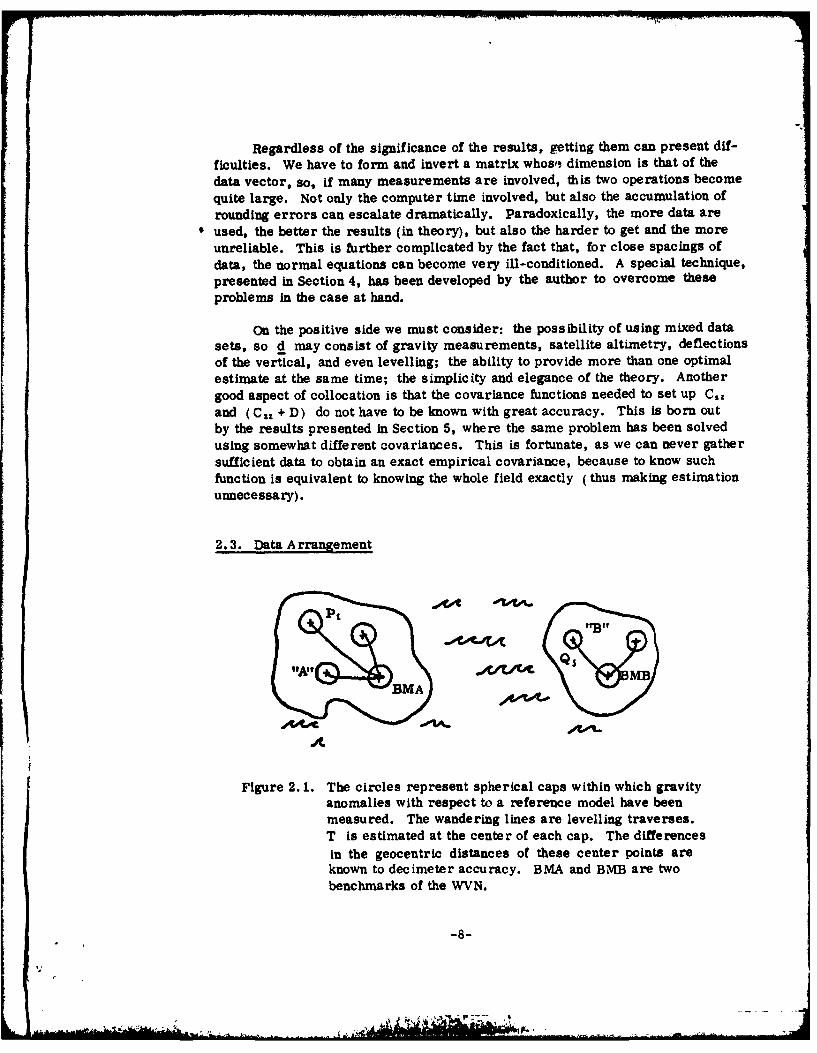
Figure 2. 1. The circles represent spherical caps within which gravityanomalies with respect to a reference model have beenmeasured. The wandering lines are levelling traverses.T is estimated at the center of each cap. The differencesin the geocentric distances of these center points areknown to decimeter accuracy. BIMA and BMB are twobenchmarks of the WVN.

-8-

Figure 2. 1 shows the basic data arrangement to be studied. While for thesimulations of Section 5 all caps are supposed to have the same size, to reducecomputing, this is by no means essential. Other kinds of Information (such assatellite altimetry) could be included among the data (see, for instance, paragraph5.3), though only the types indicated in Figure 2.1 shall be considered here.Anomalies are determined at the Earth's surface, somewhat in the manner of

Molodenskii. Details are given in Section 3.

2.4. Adjustment Theory

Consider a cap center Pt in zone "A" (Fig. 2.1) and another Q, in zone"B". The potential difference between benchmarks BMA and BMB is

AAW (BMA, BMB) = U (PI) + T (PI) + AWe (BRA, P1) + OWL) - U (QJ)

T(Qj) - AWf(BMB,Qj)-0(Qj)-Vij (2.17)

whereV1j = (4W,(BMAPt) - fAWt(BMB,Qj) + cU(P) - EU(Q 3 )

A A+ fT(PI) - fT(Qj)

is the sum of the error in levelling f W, the error in the potential according tothe reference model cU, ard the error in the estimated disturbing potential C T.cU is influenced both by errors in the model and errors in the coordinates of theP1 ,Q.. Expression (2. 17) can be regarded as an observation equation with thepotential difference A W as the only unknown. Each pair of caps (Pi,Qj) pro-vides an equation of this kind, so a redundant system can be set up

aW(BMA,BMB) = p+ v (2.18)

where p is the vector of "observed" potential differences, v is the vector orresiduals, and a is a vector with all components equal to 1 : the design "matrix"of this particular system. All three vectors have for dimension the numberof equations. This number is restricted by the following considerations: the

centers of the caps, paired in the same way as the caps, should not form a closed

loop, as shown in Figure 2.2 by a broken line. Otherwise, because the "observed"values for the pairs in the loop always add up to zero, i. e., are linearly dependent,the a priori variance-covariance matrix of the "observed" values must be singular.

As explained in Section 2.1, errors in o(Pz) and o(Q:) due to errors in the co-ordinates of P,, Qj, and in the rotation rate w, are considered to be negligible here.

-9-

The inverse of this matrix is needed for the adjustment of AW, so this limits thechoice of pairs of caps to those not forming loops. The number of such pairs isone less than the number of caps, and this is also the maximum number of equationsin system (2.18).

P P P PS "A"I

Q2 Q3 Q4 '"B"

Figure 2.2. The solid and broken lines identify capsthat have been "paired". The broken lineshows a selection containing a loop (notpermitted). The maximum number ofequations (permitted) = number of caps-1.

The accuracy of AW(BMA,BMB) after the adjustment can be computed from thefollowing formula

(No No (V'l)k (No no. of equations (2.19)Wno. of caps- 1)

where V, the variance -covariance matrix of the data, is

V = V + V(~ + VEA (2.20)

In this expression,

V4A. is the variance-covariance matrix of the levelling errors;VEAu is the variance-covariance matrix of the errors in U (PI) -U(Qj);VcP is the variance-covariance matrix of the errors in I(PI) -f (Q).

The uncertainties in AW, and AU depend on those of the data that give themorigin; C hA' depends also on the way T is estimated from the gravity anomalies.

-10-

I".

• ~~*Y~. - ,

• , +. : ....

3. Characteristics of the Data

In this section we shall consider those characteristics of the data that affectthe accuracy of potential differences adjusted according to the method explained inthe previous paragraph. The various types of data involved are: position fixes,the coefficients of a reference gravity field model, gravity anomalies, and levellingtraverses.

3.1. Position Fixes

To compute the reference potential U at the center of every cap, it isnecessary to know the coordinates of these points. The reference model containsterms below degree 20 or 30 (in this study) so the smallest detail it can show isof the order of 1000 km. U is, therefore, a smooth function of latitude and longi-tude, and cannot be substantially affected by horizontal position errors of the orderof less than 2 m, which is the accuracy that can be obtained at present with satelliteDoppler techniques. The reference potential, on the other hand, is quite sensitiveto vertica (geocentric distance) errors, at the ratio of about 1 kgal m permeter of error. As we are concerned with finding potential differences,the most important errors are those in relative vertical position. To beprecise, the vertical position of interest is the distance to the geocentre. Thereis little difference, however, between relative errors in ellipsoidal heights andrelative errors in geocentric distance, and both can be regarded as equivalent here.The absolute vertical error might contain a nearly constant bias, due to the incor-rect dimensions of the reference ellipsoid and to other systematic causes relatedto the positioning method. This error may be of several meters without any notice-able effect on the estimated potential differences, because it will nearly cancel-outwhen such differences are between points at the Earth's surface. Therefore, anerror in the ellipsoid of the order of 2 m, which is the present level of accuracy,can be disregarded.

While the relative vertical position error is the one that matters, we stillhave to know the absolute geocentric distance to compute U. This can be done,essentially, in two wayss

t

- L-11-

I

it!2

a) find the absolute position of each point separately;

b) find the absolute position of one point, and then obtain the relativeposition of the other points with respect to this one.

In each case, the relative position errors will vary, the choice being alwaysthe alternative that gives the smallest errors.

This study is more concerned with forthcoming developments than with thepresent state of affairs: Anderle (1978) has estimated that the Global PositioningSystem currently being deployed could provide, when all the satellites are oper-ational in the mid-Eighties, relative positions with errors of less than 0.1 m.This accuracy should be possible between stations thousands of kilometers apart,in all three coordinates, after less than one day of constant observation of thesatellites. Estimates for absolute position determinations from lunar rangingstations made by Silverberg et al. (1977), using mobile stations supported by anetwork of a few fixed ones, are also in the decimeter range. In addition tothese two, a variety of new positioning techniques based on satellites in highorbits that carry laser reflectors, mobile radiointerferometry, etc., beinginvestigated at present, might provide even better accuracies in the comingdecade. Present measurements from Doppler satellites have errors that areone order of magnitude worse. However, considering the progress made in thisfield over the past decade, and the new highly precise methods in the offing, itis probably not too optimistic to assume in this study relative accuracies as goodas one decimeter in vertical position.

3.2. Reference Model of the Gravity Field

The coefficients C,,,Sn, and the constant GM in (2.1) are not exact values,so the model does not represent to perfection the first N harmonic degrees ofU or T. The effect of an incorrect GM is, at the present level of accuracy,equivalent to a bias of about 1 3 m in geocentric distance (Lerch et al., 1978).This error, being virtually constant, has a negligible effect on potential differences.The existence of coefficient errors

Z!n C .(re a(9ade19" 9m i. (true) - '9,. (ode

i) (3.1)

has to be considered when defining the disturbing potential'

The 0 degree error CGM/r, being almost constant on the Earth's surface hasno relevance to this work, and has been excluded from these formulas.

-12-

~3:7,i.

IN

T(P) =V(P) -U(P) =r ZF~ (75' P.(iflp)I(CD.C05mAp + c9,,sinmi).J

(,as~h (3.2)+ -0lmJ

and the gravity anomaly

£ N

~g(P) )T(P) T P)_GM8r r y7(P) rp 2 rp 1

cc'It

11(i'(n - )Z !P.(s in o) C cos m). + 9,.s in mX,]}

3=0 (3.3)

The corresponding isotropic covariauces, according to expression (2.13) are

C)6tP( 7_ I+ 2+ 1)6.P,(cos Vk )( } (3.4)rp rq L rp; Q

N a ' a'Cr~~~~gf (Pl~n Q)=1f )~2n 1 f1)~eCO.)f(.6

CaaPQ) = 7 ,P(cosoq + 5 1)(2n+l f6Pcs)q (3.5)

knw as , ua' rue) or suc as

(? ~a+E n3 ))' /( 2 R (3.8)

Ing ate, avaiaber icnforto n the p)akower spcrm rvit anmalirees.uTdelt6o,, cand prxtdb the hoiznalgrdentonraiy, diona ndnto the paaeesaBposterio r thinc-at iemrxo the aetditjuschinomtn this prued ofe foulshThe adanage ta thl oe a less.4, 3 a nd (3.i6)dcn e scmuh usin

finite8 re u s o s - 1 - 1

(ga - .7,n + )---1( A)+1 - 1)n-2n

Thsls xrsin totrslw, a enivsiae yIkl 17)

3.3. Propagation of Position Errors through the Computed U

Because of the low degree of the terms in the expansion of U, horizontalerrors in 0 and X are of little importance. The vertical errors Er, on the otherhand, have a s ignif icant effect. if they are small, we can write

(E U (P, Q) U (P) -U(Q)~[ U. (P) U., -U (Q) (1'(3.9)

where U. is the nthi harmonic of U. Calling

6 U.(P, Q) = U. (P) - U. (Q)and

we havetF fr

f A U, 2 2(n + imx{)IUA 'E krl (3.10)

whe re r = mm inrn , rq) and ) a (r, 2) is the su rface of the sphere a( r,O)0 S ince

UO ~tl~o) F iUdtL

for n > 0, it follows that

for n > 0. Calling

v (rp + 'E, P+ rQ + Cgwe get

IU IEo U" GM I C, 1~ * (3.11)

where '7 is the mean value of gravity acceleration on the Earth's surface(~0. 9798 Kgal). The standard deviation of ecA U is

'EAU 'Y a(r~q(3.12)

-14-

If the coordinates of points P and Q were determined separately, so e rp and

crQ could be considered uncorrelated, and if ae rp = ae rq = a er then

a Eau VTa C (3.13)

On the other hand, if the difference in vertical position is determined simultaneously

for P and Q, then (3.12) applies. In any case, if all geocentric distances arecomputed with uncorrelated errors, except for some constant bias that does notaffect the potential differences, then matrix V.Au in (2. 20) must be diagonal,

each non-zero term being

v1 1 t I OAu, (3.14)

where Au1 is the potential difference between the centers of the ith pair of caps.

3.4. Gravity Anomalies

The theory used in this work assumes that the exterior potential of gravi-tation is harmonic. This is not strictly correct at the Earth's surface,because of the atmosphere above it. To avoid systematic errors this

effect should be discounted from the measured gravity values, and put back on

the estimated potential. These atmospheric corrections have been studied in

detail by Christodoulidis (1976). Probably, the variation in gravity due to Earth

tides and ocean loading should be corrected as well, in order to achieve the

degree of accuracy required here. Another source of systematic error is thegravity net to which the measurements are "tied". As explained later, system-

atics of more than 0. 1 mgal rms are undesirable, so the contribution from the net

should be as small as possible. Master stations where absolute gravity is knownto, say, 0.01 mgal would be quite adequate. Of course, a constant bias due to an

error in the nets' datum has no effect on the estimated potential differences, and

can be ignored.

A further cause of systematic errors in the gravity anomalies are the

distortions in the levelling net to which the stations are tied. The influence of

such distortions on estimates of the disturbing potential have been explained

by Lelgemann (1976). We are going to study here a way of determining the anom-

alies that minimizes this influence.

Besides actual errors in levelling, the main reason for distortions in vertical

nets is the use of tide gauges as benchmarks. Their mean sea level marks are

supposed to be at the same potential, and the net is adjusted with this as a constraint.

In reality, the stationary sea surface topography already mentioned is present,

-15-

and the potential differences among gauges are not quite zero. These discrepanciespropagate as errors throughout the adjusted net. The larger the network, thelarger the distortions can be, and also the longer the distances over which theyare correlated. To shorten this correlation length we shall break the existingnet into smaller pieces, and to eliminate the effect of the sea surface we shallnot use a net that is adjusted with constraints based on tide gauges. To achievethis we are going to use the center of each cap as the levelling datum for all thegravity stations inside that cap. The potential of each station is going to bereferred, accordingly, to the center point. Since the caps considered here aresmall (50 and 100 semi-apertures) the levelling net for each cap will consistonly of short traverses whose measurement errors can be ignored. If necessary,the net inside each cap can be adjusted, to filter out such errors. To use theestimated potential of each cap center in our vertical connections, we have torefer all of them to some common datum. To do this without reverting to theuse of tide gauges for this purpose, we shall take advantage of the accurateposition fixes taken at the cap centers, and find the reference potential U ateach one of them. f we take the U (Pt) for the true potentials, we make amistake quite similar to that of assuming that all tide gauges are on the samelevel surface. The errors, however, are proportional to the T(PI), thequantities to be estimated. As shown below, this leads to equations that can besolved for these "errors", to obtain the desired T (P 1 ) free from biases. Ina way, it can be said that the centers of the caps are the equivalent of tide gaugesin the adjustment of the World Vertical Network.

A gravity anomaly Ag, in terms of the reference model, is

Ag(Q) = g(Q) - Y(Q') (3.15)

where g(Q) is the acceleration of gravity measured at a point Q on the Earth'ssurface, and y(Q') is the model's acceleration at a point Q' such that Xq = XQ,and oq = oq,, while U (Q')+o(Q)= V(Q) +,D(Q) = W(Q). The rotationpotentials O(Q) and O(Q') are almost equal, because the difference ( - rQ,)is of the order of 3 m for a reference model up to degree and order 20. For thesame reason, the linearized expression

Tg(Q) + 7 r ( (Q) (3.16)

can be regarded as almost exact. These approximations hold better for this typeof model than for the simpler, and traditional, ellipsoidal model. The gravitypotential at the gravity station Q is

-16-

A!

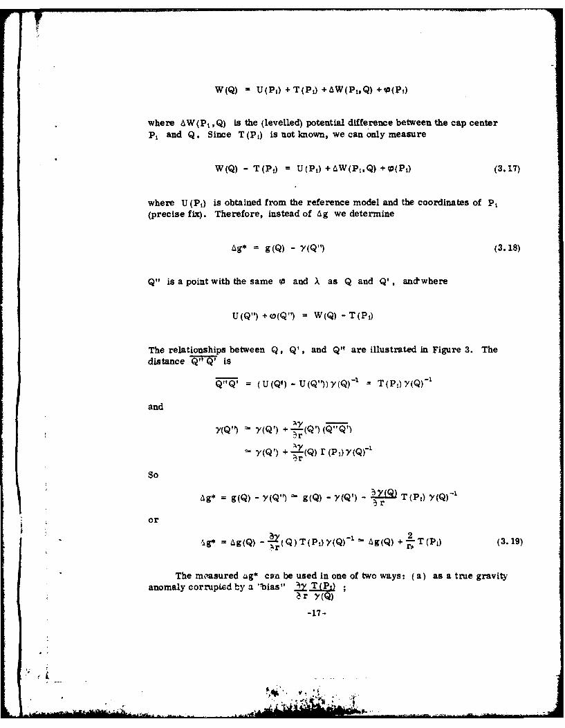
W(Q) = U(Pi) +T(Pi) +AW(P,Q) +O(Pi)

where AW(Pi,Q) is the (levelled) potential difference between the cap center

P1 and Q. Since T (PI) is not known, we can only measure

W (Q) - T (PI) = U (P) + AW(PIQ) + O(P) (3.17)

where U (PI) is obtained from the reference model and the coordinates of P1

(precise fix). Therefore, instead of Ag we determine

Ag* = g(Q) - Y(Q") (3.18)

Q"? is a point with the same 0 and X as Q and Q', and where

U(Q") +w(Q') = W(Q) - T(P 1)

The relationships between Q, Q', and Q" are illustrated in Figure 3. Thedistance Q" Q' is

QQ' = (U(Q)- U(Q"))y(Q)' = T(P )Y(Q)-'

and

Y(Q'Y) " y(Q') + R() (

y (Q) + -Y(Q)r (P)v(Q)'

So

Ag* g g(Q) - y (Q 1) -g (Q) - y (Q ) Y Q T (P1) Y(Q) 1or

= g((.. ci.ri )In _2(3.19)

g, = Ag(Q) - (Q) T (Pj)(Q)-I Ag(Q) +-T(PI)

The masured ag* can be used in one of two ways: (a) as a true gravityanomaly corrupted by a 'bias" 2z T (P)

~r y (Q)

-17-

.,.. v.

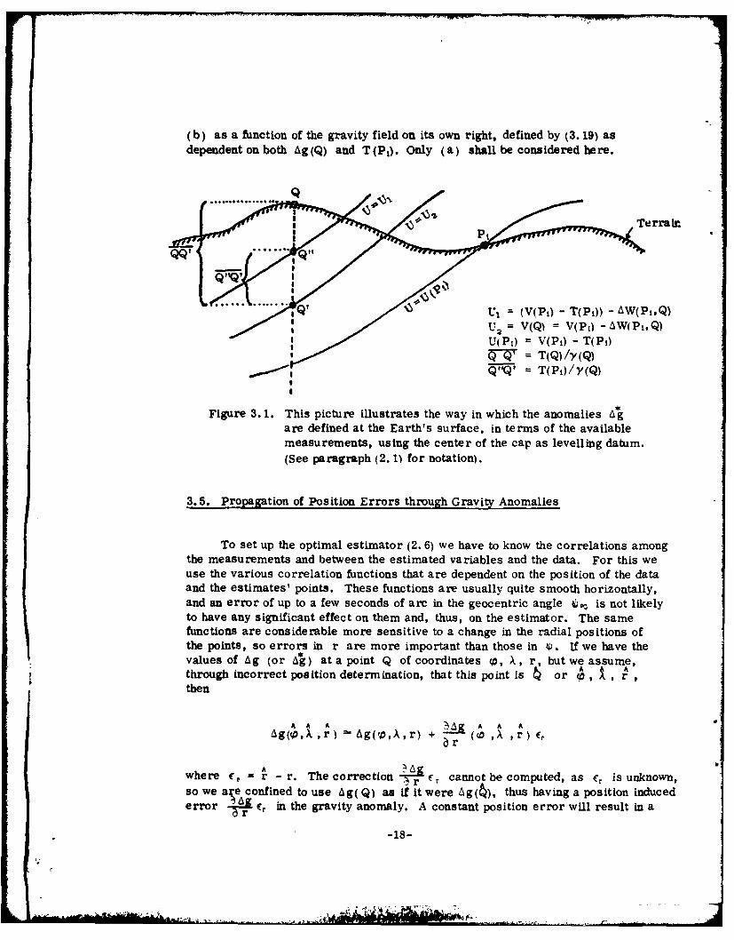
(b) as a function of the gravity field on its own right, defined by (3.19) asdependent on both Ag(Q) and T(PI). Only (a) shall be considered here.

I Terrain

IU 1 = (V(PI) - T(Pi)) - AW(Pt,Q)U = V(Q) = V(P) -AW(Pt,Q)U(PI) V(P) - T(P,)Q- = T(Q)/y(Q)

SQII = T(P)/y(Q)

Figure 3.1. This picture illustrates the way in which the anomalies a*are defined at the Earth's surface, in terms of the availablemeasurements, using the center of the cap as levelling datum.

(See paragraph (2. 1) for notation).

3.5. Propagation of Position Errors through Gravity Anomalies

To set up the optimal estimator (2. 6) we have to know the correlations amongthe measurements and between the estimated variables and the data. For this weuse the various correlation functions that are dependent on the position of the dataand the estimates' points. These functions are usually quite smooth horizontally,and an error of up to a few seconds of arc in the geocentric angle M is not likelyto have any significant effect on them and, thus, on the estimator. The samefunctions are considerable more sensitive to a change in the radial positions ofthe points, so errors in r are more important than those in j. If we have thevalues of Ag (or Ag) at a point Q of coordinates o, X, r, but we assume,through incorrect position determination, that this point is or 4, X, ,Pthen

A A A A A AAg(o ,,r) A'Ag(,o,),,r) + Mag ,X ,r) i

A Agwhere c0 = r- r. The correction r c, cannot be computed, as c, is unknown,so we are confined to use Ag(Q) as if it were Ag(4), thus having a position inducederror " e, in the gravity anomaly. A constant position error will result in a

-18-

+'+' +" ' + + ' + 'M ' + W +:' + 'I~r""+:++++, :,'.., . .... ... m+}.+lm~m++ ... . .... " '' +. .. ++:, .+.: .... • ... ,m,, ,+ :. ..... ... ... ......+ "

constant bias in all gravity anomalies, as the variation of - r over the whole rangeof r on the Earth's surface (about :30 kin) is very small. An error in Ag will,in turn, propagate into the estimated T's

Nd A

T E f,(Ag + AgL) =T +Eft cag, = +O(cYC6~I)I.=O I

If the data arrangement is much the same for each cap, then the estimator "weights"f1 are also much the same in any cap, and the resulting error in each T froma bias in Ag is going to be nearly constant. These nearly equal errors in potentialwill very likely cancel-out when potential differences are computed. For the samereason, the effect of an erroneous GM on the mean value of the reference model'sgravity will not have any appreciable consequence on the estimated potential differ-ences. Thus we can have rather large biases in GM and on the set of stationpositions (error in the size of the reference ellipsoid). On the other hand, lesscorrelated errors in r are not likely to cancel out. However, the rms valueof at the Earth's surface is approximately only 8 pgals m - . From the resultsin section 4 it follows that errors up to 0. 1 mgal in Ag, which are highly system-matic inside a cap but vary randomly from cap to cap, can be tolerated. The sameresults show that several regal in errors totally uncorrelated from station to stationhave very small effect on the accuracy of T. From all this, it can be concludedthat: a) errors of several meters in r (at gravity stations) constant over the wholeEarth, can be tolerated;

b) errors of several meters in r, constant inside each cap, but uncorrelatedfrom cap to cap, are acceptable;

c) errors of several meters in r, uncorrelated from station to station havesmall effect.

The Global Positioning System, already mentioned, is expected to provide fixesaccurate to 10 m in each coordinate after six seconds of receiving radio signalsfrom four satellites visible at the same time (Anderle, 1978). After 15 minutes,this accuracy should improve to 1 m, plus a constant bias of no more than 3 mdue to an error in the adopted ellipsoid. Thus, the contributions from (b) and(c) above should come to about 1 m, guaranteeing negligible position inducederrors in Ag. By using a GPS receiver in conjunction with a gravimeter, onehelicopter crew could collect all necessary information within a 50 cap (about500 stations) in less than two months. Additional work would be needed to estab-lish levelling ties between each station and the prediction point at the center,for which already existing traverses could be used, where available. In fact,

even without G PS fixes, the positions of points like Q" in paragraph (3.4),which are obtained using levelling and the reference model, can be used as station

positions. The errors are going to be

[V(Q) -U(Q")]/) 1 " (T(P,)- T (Q))/GMa- 2

-19-

7W'

If a 20,20 model is used, the rms of T will be on the order of 3 kgal m, soCrQ /2 x 3 kgal m. Because potential is a smooth function of distance, thecorrelation c TT between T (Q) and T (Pi) will reduce the rms of the error

a' CrQ = (4aO"(T (Q))3 + a (T(P)) - 2 C TT (0 PQ, rp ,

over distances of the order of one cap radius (500 km), so levelling-determinedpositions might be sufficient for the gravity stations. L

3.6. Levelling

Levelling is needed to connect cap centers to benchmarks, and cap centersto gravity stations within their respective caps. Existing traverses should be usedwherever possible, but only unadjusted values or values adjusted within relativelysmall regions must be used. Otherwise, results could be biased by the distortionsaccumulated in large adjusted nets. To keep errors small, the traverses should beas short as practicable. This goal is easily achieved for the levelling inside caps,as distances from center to rim range between 500 and 1000 km in the cases con-sidered; the longer traverses from centers to benchmarks require a careful planningof the overall system. Caps should be placed, as much as possible, within flat areaswith a smooth field of gravity anomalies, because estimates of T are likely to bebetter there than where both field and terrain change wildly, as suggested by theresults in Appendix A. Traverses should be levelled across regions where thetopography is gentle, to reduce their errors.

The simulations reported here have been done assuming that all levellingtraverses run along arcs of maximum circles, that their errors are uncorrelatedunless they overlap, and that the standard deviations of these errors obey the simpleformula

a.W. = 0. Iv kgal m (3.20)

where i is the length of the traverse in thousands of kilometers. This formularepresents a quality of measurement not much better than that of present day firstorder levelling (see, for instance, Lelgemann (1976)).

An error c., will result in an error ycr kgal m in U(P);,of about 0.3 cpregal in the value of each A* ; and of approximately 0. 3 c,, 1 :f kgal m inTo. However, according to Tables 4.3 and 4.4 f, 0. 3 for 5 and 10" caps,so eT, due to c is 0(0.1 r,) kgal m and can be neglected here if Co< 0.5 M.

-20-

4. Computing Disturbing Potentials

Paragraph (2.2) explains the choice of least squares collocation as the tech-nique for predicting T at the cap centers. Several practical problems associatedwith this method must be considered before even relatively simple simulations canbe carried out. A description of these problems and their treatment is given inthis section.

4.1. Reducing the Dimens ion of the Data Covariance Matrix

Assuming that the gravity stations are spaced some 40 km from each other,then their number in each 50 cap will be close to 500, and to 2000 for a 100 cap.This means that C,, + D is either a 500 x 500 or a 2000 x 2000 matrix, respectively.Being symmetrical, it will have up to 2000000 different elements for a 10 -7 cap,each one requiring one calculation of the covariance function c.... ( p, Q). Thiscan be a very costly process in terms of computer time, and inverting C,, + Dcan be costly as well. This is particularly true in the context of a study in whichcalculations may have to be repeated several times with slightly changed assump-tions. For these reasons an arrangement of the data was chosen that gives theCfz + D matrix a strong structure. This, as explained in Colombo (1979), bringsabout great savings in both forming and inverting the matrix. To understand howthis is possible in our case, consider the following argument. Imagine that thegravity measurements are arranged in concentric rows around the center point,which is also the estimation point, and that all stations are on the same geocentricsphere as the center. Instead of the individual anomalies, suppose that we usethe row sums

E--=

as data. The number of Eg' s is the same as that of the rows, N,. The covariancefunction for the Sg s is

N1 NJ

cg '[(i,j) Mfhgi Agi = n._4_1 Mf{g'. Agi (4.1)

(N ,NJ are the numbers of stations In rows i,j) while that between T( P) andhg 1 is

N!

c (p,i =) . ;I(1gjpj = N:M(Thgjjj (4.2)

as M(Tag j is constant for all stations in the same row.

-21-

With these two functions we can set up C,, and C,, while the noise matrix is

D {d : 2 i (4.3)dii =

where at. is the standard deviation of the mth measurement on the ith row. Cz,is now only N, x N, : for a 50 with 40 km between rows, N, = 13. This implies areduction of more than one order of magnitude in the dimension of the data set andof several in computing time, because setting up the matrix is proportional to its(dimension) , while inverting it requires a time proportional to (dimension)3 . More-over, as shown in the reference given above, if the points are equally spaced alongeach row, having the same number in each row, then estimating T from g orfrom Ag gives the same result. In other words: this arrangement largely improvescomputing efficiency, without changing the quality of the result.

A distribution of data with the same number of points in every row is not agood one, because if the maximum separation (in the outer row) is 40 kin, thenthe stations will be very crowded at the center. If points are eliminated to thinout the central region, the exact equivalence to collocation using Ag will be lost.This will bring some deterioration in results, though not a very remarkable one.The actual accuracy can be found, as usual, using expression (2.11) and the matricescorresponding to g 's. The unequal number of points will result in the outer rows'covariances being larger than the central ones', and this will probably worsen the con-dition number of the matrix. To avoid this problem, the row sums can be replacedby row averages.

Ag1 A Ag'. (4.4)

The covariance functions for these are

=~1 ~~ MrAg 1 Agj } (4.5)

N1

cTG = MfT(P)Eg&j = M MfT(P)Ag,9 = M(T(P)Agj) (4.6)

and= 7 Crm, D being diagonal. (4.7)

The grids used in this study were constructed according to a simple pattern thatkeeps average distances between stations at about 40 km. There is one station atthe very center, six in the first row, twelve in the second, twenty-four in the third;their number doubling from there on every time the diameter of.the row doubles (at

the 3rd, 6th, 12th, row, etc.), and staying constant otherwise. Figure 4. 1 showsthis scheme used on a cap. In such a grid, the separation between rows is

-22-

Figure 4.1. Arrangemeut of Gravity Stations in the 54 Cap.

4. 4 4. 4. 4. 4-4. -. 4. 4.

4+ + + + +

4 .. 4. . . 4. 4 4. . 4.4. 4-

+ 4+ 4- 4+ + + + + + 4. 4 4 + +4. 4. 4. 4 4.

4 4 + + 44 4 4 4+ + 4 44. 4. 4. 4. 4. 4-4. 4. 4. 4. 4.4" 4. 4. 4-

4. 4- 4+ 4. 4. 4. + + 4+ 4.4 4.

4 4 4.4 4- 4 * 44" 4. 4. 4. 4..4" 4. 4 4 4 4 . 4. 4. +

+4 4 4, 4. 44 .4.4 4 . .4-4.4 4, 4".

4.4 4. 4 4. 4.4. 4- 4 4. 4. "44 4 4 4 4 4.4. 4. 4-4."4.-4. 4.4.4.44. 4.4

+ + 4. + + + + 4 4 + + + + + + + + 4.4 + 4. +4 + +

.4 + 4. 4 + "t 4- 4. 4. 4"

+ -+- 4".. 4. 4 " 4 4 -- 4-

4-. 4

+ + 4- + + + .4 * 4. -4.I 4 + 4 - 4.4

+ " "I 4.- 4.4."" - + 4 4 .I - 44.-4 . + 4 +-.- 4. 4. 4

4 4 + 4 4- 4" 44. .4 4 + 4 4 . 4. 4.4.1" 4 -- + 4. 4

+ 4. 44. 4 4. 4 4- .4 4 4 4 4" 4 - 4 "

+ - 4.4

. 4.4. 4 4- 4 "

-23-

IV K.-

always almost 40 km, and the constant separation of stations in the same row varies,from row to row, from 30 km to 60 km. Furthermore, the values of the covariancebetween any point in row i and all points in row j 2 i are repeated at all points inI. This greatly speeds up the creation of Cz, as all terms such as

in (4.5) are equal regardless of m. Finally, computing time can be halved by takingadvantage of the fact that if a radial line is drawn through any point in the figureits covariances with all points to the left of this line are the same as with those onthe right.

It is most unlikely that all gravity stations will actually have the same geo-centric distances, and there is no fundamental need for this, as collocation can beimplemented with whatever coordinates the stations may have, although less effi-ciently, as long as they are known with reasonable certainty. However, if the com-puting savings mentioned above are tobe realized, the data must first be reduced to anideal grid by collocation on a spherical surface. Measurements in the vicinity of each nodeof the ideal grid can be used to interpolate a value on that node. Over a reasonablygentle terrain, the distance between it and the sphere is not likely to exceed 2 kmwithin a 50 cap, and some of the nodes are going to be below, and some above theEarth's surface. Assuming that five gravity stations were used, one on the samevertical as the node but 2 km above (below) it, and four others forming cross withthe first at the center and 20 km arms, also 2 km above (below) the sphere, theaccuracy of a value collocated on the node is ± 0.8 ingal if the data has * 0.5 mgalmeasurements' white noise. This was found using the same covariance functionsemployed in all the other simulations conducted during this study. Since collocationis a smoothing process, the rms of the estimation error is likely to be due, by andlarge, to the high frequency components of the data. As shown by the simulationsin the next section, as much as 4 regal of high frequency errors will have a neg-ligible effect on the accuracy of the adjusted vertical connections.

4.2. Estimating T from Ag instead of Ag

As already explained, the optimal estimator

AT(P,) = f d = Cz (Csz+D)-d

depends on the type of data chosen d = z + n . Let C,z and C.1 be covariancematrices for gravity anomalies Ag arranged inside a cap of center P., butsuppose that the data available consists in values of 4 with the same spatial

-24-

IItA

arrangement. According to (3.19), if T is given In kgal m and Ag in nigal,

6% = Ag +k T(P.) (4.8)

where k , 2- x 106~ 0. 3. Calling T the estimiate of T (P.) based on Ag, and+the estimate of T (P.) based on eg, and using overbars to design row averages,

as in the previous paragraph, then

T (Ps) = T(PO) + c (PO) E f, (6 g + kT(P.) k k(T(P.))]

N1. N1.

= £~f 1 ~g-kT(P.) Ef

So rN

T(P.)[1 + k I fd + f(. = 5f 1 Ag(4.9)

and N

A(. A i 1 lfia' (4.10)

Consequently, N1.

IE(a (Pe) if E f1 > 0 (.1a1= 1

N.A1E(Pa) -- 7(P.) if )f, !5 0 (4. 11-b)

Nr

IfZ-f > 0 there is a reduction In the estimate's error, according to (4. 11-a),adthe opposite happens when f, 0 0, according to (4. 11-b).

-25-

4.3. Accuracies for T (P,) Estimated over 50 and 100 Caps

Tables 4. 1 and 4.2 show the accuracy of T estimated under different con-ditions, using the theory explained in the two preceeding paragraphs. To obtainthe theoretical accuracy, and for the reasons given in the previous paragraph, thesquare %oot of the value calculated according to (2. 11) was corrected by the factor( 1 +k trf 1 )- 1 . While varying slightly from case to case, this factor is alwaysclose to 0.9 for 50 caps, and to 0.8 for 100 caps.

The values of the "weights" f (i.e. the components of _) do not changegreatly, under varying circumstances, from the "typical" ones listed in Tables4.3 and 4.4. This is particularly true of the largest "weights", from the centerpoint to the 10th ring, which remain nearly constant.

In general we can say that, for a 20,20 model and up to several mgal rmsof white noise in the gravity data, the accuracy of T estimated on a 50 cap isclose to 0.4 kgal m, and for a 100 cap It is near 0.3 kgal m.

The "imperfect model" used for the results consists of the first N degreeharmonics of a 180,180 model obtained by Rapp (1978b) as a combination of a worlddata set of 10 x 10 gravity anomalies with GEM-9. The standard deviations of thecoefficients are listed up to degree N = 30 in Table 4.5. The "2L" and "2H'covariance models are based on formula (3.8) and have the following coefficients(Jekeli, 1978):

2L 2H

A = 100 at = 18. 3906 mgal 2 A = 140 at = 14.0908 mgal2

B = 20 u = 658. 6132 mgal2 B = 10 oa = 160.670. mgal2s, = .9943667 s, = .9939083s 2 = .9048949 sa = .9997595

where 2 an(A)2 and

Covarlances were computed with these coefficients and the closed expressionsalso given in the above reference. To simplify calculations, all measurementsand estimations are supposed to be made on the same sphere of radius a = 6371000m. To test the resulting accuracies, some numerical experiments were conducted,as reported in Appendix A.

-26-

17

Table 4.1.

Accuracy of Estimated Disturbing Potential (kgal m) for 50 Caps and "42 L"Covariances (some values obtained using "2 H" are in brackets).

Imperfect Model Perfect Model RMS of cat Maximum Degree,in mgal Order in Model

0.81 0.80 2 10(0.37) 0.41 - 4 20

(0.36) 0.39 (0.23) 0.27 2 200.38 0.27 0 200.40 - 4 300.37 0.21 2 30

(Values estimated from Lg's are 1/0.9 of those given here.)

Table 4.2.

Accuracy of Estimated Disturbing Potential (kgal m) for 100 Capsand 1"2 L" Covarances

Imperfect Model Perfect Model RMS of cdk Maximum Degree,

in mgal Order in Model

0.29 4 200.27 - 2 200.24 0.19 0 20

(Values estimated from Ag's are 1/0.8 of those given here.)

-27-

.

-, , :,, , '

Table 4.3.

Optimal Row "Weights" fi (kgal m/rgal) for 50 Caps, Maximum Degree andOrder in Model is 20, RMS of ( g is 2 mgal (all values multiplied by 0.1).

Row No. Imperfect Model Perfect Model

t12 L" 112 H" "2 L" " 2 H"

fIxO. 1 fjxO.1 fjxO.1 fxO.1

0 (center) 0. 225 0.225 0.225 0.2241 0.438 0.438 0.436 0.4352 0.408 0.409 0.404 0.4023 0.388 0.391 0.383 0.3804 0.351 0.354 0.344 0.340

5 0.301 I 0.304 0.292 0.2876 0.301 0.307 0.290 0.2857 0.255 0.260 0.242 0.2378 0.228 0.234 0.214 0.2089 0.198 0.204 0.183 0.176

10 0.176 0.182 0.158 0.15011 0.122 0.129 0.109 0.10412 0.234 0.243 0.189 0.168

From these values it is clear that a constant error in gravity ego (mgal) willresult in an estimation error (bias)

12To = e go Z ft 0.3 cg kgalm.

1=0

Table 4.4.

Optimal Row "Weights" f, (kgal m/mgal) for 100 Caps, afalg = 2 mgal, ImperfectModel to Degree and Order 20, "2 L" Covariance Function.

Row No. fx0.1 Row No. f f~x0.1 Row No. ftx0.1

0 0. 2181 0.434 9 0.294 17 0.153

2 0.419 10 I 0.276 18 0.1383 0.413 11 0.241 19 0.1234 0.392 12 1 0.252 20 0.1105 0.352 13 0.218 21 0.0976 0.368 14 0.204 22 0.0857 0.331 15 0.186 23 0.0738 0.316 16 0.169 24 0.059

25 0.110

-28-

AAA

Table 4.5.

Accuracies of the Potential Coefficients in the Imperfect Model, by Degree.

n 1n n

x 10 - 1 x 10 "1, x I0 "l 1

1 - 11 4990. 21 2899.2 2720. 12 4415. 22 2761.3 6594. 13 4830. 23 2635.4 4564. 14 4458. 24 2522.5 7237. 15 4140. 25 2417.6 5703. 16 3864. 26 2321.7 6707. 17 3623. 27 2232.8 5685. 18 3410. 28 2149.9 5727. 19 3220. 29 2072.

10 5118. 20 3051. 30 2001.

4.4. Correlation Among Estimation Errors

The elements of matrix V E2 (expression (2.20)) are of the form1

A A A a A A AVkk = M(C T(Pik) - € T(Qjk))2 = 0' C T(Pi) +0'E T(Qjk)- 2Mf T(Ptk)( T(Qjk) )(4.12)

if the element is on the main diagonal, or

v. = M(,ET(P1 -CT(Qj )(cT(Ptm) -fT(Qj)) (4.13)

= Mf "T(Pt.) c T(P,,)) + M ET(Q,) ( T(Qj,)) - Mf( T(P.)(P.),E T(Qj.) }

if it is off-diagonal. To simplify matters, let us assume that all caps are of thesame size and have the same data distribution inside. Then

where a is the global rms of the estimation errors, found in accordance to (2. 11).Furthermore,

The subscript k indicates the "caps pair" or observation equation number.

-29-

'*'

Mr(T(6) (T(Qk) = M(T(P,) -fdj)(T(Qk) -IfT dk)))

= CTT,(P6,Qk) - 2Cr k, 1, C!L 1 lf (4.14)

where d = [Ag 1 ,Ag ,. gt,...,A,,]hr corresponds to the hth cap, and

CTI 1, = M(T(Ph)dkr?

is a 1 x D4 row vector (Nr is the number of concentric rows in each cap)

C Ih t = M[!d

isa N, xNK matrix (. is the data in the hth cap).

The elements of these matrices are:

N,

C, = M(T(Ph)EAg 1 (k)) -L-MIT(Ph) Ag(k)3

N- M(T(,)AgL(k)) (4.15)

for CTK

(where Ag .(k) is the value of Ag at the rth gravity station on the ithring centered at Pk), and

NNC tj = M(S=gik) 'gj(h)) = -R'N, M( a gir(k) Z Agj.(h)}

= N r gj~)Aj s' (4.16)

for C_.

If the total number of caps is N,, there are approximately (1/4) N.' N,.different

"ring covariances" (the general term in (4.16)), and each requires computing the

covariance function of Ag Nt x Nj times. This can tax the largest computingbudget; on the other hand VCA is only part of the a priori variance -covariancematrix used for adjusting the potential difference between benchmarks AW(BMA, BMB).Usually, a priori covariances are not needed to very great accuracy, because theadjusted values are not extremely sensitive to them, or should not be if the procedurehas been designed properly. f approximate values are enough, then a most efficientway of obtaining them, correct to several significant figures, is to assume that thecovariance of the "ring averages" Ag1 (h) Ag4 (k) is

-30-

L..14,i

M(Sg9(h) -g,(k)}" M{ 2 a1 n Iag(O,,v)d - 1 401

a E (2n + l)(n -1)a 8c P,(i4) P,(uP) P,(4) +

+ (n 1(n- 1' n n, I) P1(0wp&) J(4. 17)

where 41 is the spherical distance between the centers of the caps where ringsi and j are located; 0 , and ,, are the sizes (semi-apertures) of rings i andj ; while N, 6 c,, 8 8 are the same as in expression (3.4). Values computed asabove are accurate to no less than three significant figures foj Od > 0"

0 , 01,

*j < 50 and N..a > 400. Table 4.6 presents values of M[e T(Pk) cT(Pj) 3 for

different distances between cap centers: this illustrates the considerable indepen-dence of estimates separated by more than 2000 km. As the data are supposed tobe ag's rather than Ag's, results have been divided by 1 +0.3 1 fi" 0.9

Table 4.6.

Correlation Between Disturbing Potential Estimates at Various Distances(0 cAg = 2 mgal, 50 Caps, Imperfect Model up to Degree and Order 20).

M [cT(P )ET(Pj)} (kgal m)a Distance Pj P-

"2H' "2 L" km

0.130 0.154 00.032 0.033 11500.027 0.028 13000.008 0.007 20000.002 0.002 2300-0.002 0.002 25000.001 0.002 14000

-0.002 -0.002 17500

5. The Accuracy of the Adjusted Vertical Connection

This section presents the main results of this study: the theoretical accuracyof a World Vertical Network constructed along the lines already discussed. It alsocontains the theory of an optimal estimator for potential differences between centersof pairs of identical caps, and other ideas regarding possible uses of satellite andterrestrial data for setting up and strengthening levelling nets.

-31-

5.1. Transoceanic Connections Using Several 50 Caps

Two cases have been considered: in the first, five 50 caps were placedin North America (4 in the U.S. and 1 in Canada) and another four in Australia.The cap centers have been chosen to avoid overlaps and to ensure that almostall the area covered by the caps is land. The 'benchmarks", two points whosecoordinates are given below, are: BMA in Electra, Texas, and BMB in Wiluna,Western Australia. Cap centers in the same land mass are supposed to be joinedto the corresponding benchmark by levelling traverses, as in Figure 2. 1. Toassign a standard deviation to the error of each traverse, formula (3.20) hasbeen used, the length of the traverse being that of the maximum circle joiningits endpoints. All data is supposed to have been measured (or reduced) to thesame sphere of radius a = 6371000 m to simplify calculations. Tables 5. 1 and5.2 show the accuracies obtained using formula (2.191 with the "a priori" matrixV corresponding to various combinations of covariance function and referencemodel. The following is the list of cap centers, including their latitudes (thebenchmarks are also cap centers). The difference between the North America/Australia and the U.S./Australia connections is the fact that cap number 9 inthe former has been replaced by cap 9* in the latter.

Cap No. Latitude Longitude Location State

1 (BMB) -27.5' 120.00 WILUNA W. Australia2 -20.0, 130.00 Tanami N. Territory3 -22.50 142.00 Middleton Queensland4 -32.50 145.00 Cobar N. S. Wales5 36.00 -85.5" Sparta Tennessee6 (BMA) 34.50 -99.00 ELECTRA Te:as7 44.00 -99.00 Wessington South Dakota8 37.00 -112.50 Fredonia A rizona9 56.50 -112.00 Mc. Murray Alberta9* 65.00 -150.0a Manley Alaska

Overall, the accuracies listed in Tables 5.1 and 5.2 can be separated into twogroups: those based on the use of an imperfect reference model, and thoseobtained assuming a perfect model. Results within each group are much thesame: approximately 0.3 kgal m accuracy with an imperfect model, about 0.2kgal m with a perfect one. Changes of 100 in the accuracies of levelling orgravity measurements caused less than 10% variation in oaXW (the effect of lev-elling accuracy is shown in Table 5.2); while a change In covariance model hadonly a slight effect on AW, as suggested by the components of the respectivepseudoinverse vectors v listed in Table 5.3 (where vrp = AW, see paragraph(2.4)), and as shown in Table 5. 1.

-32-

In summary: the accuracy of the reference model is the most important of thevarious sources of error included in this study. Improvements in this modelare likely to have a large effect on the quality of the resulting vertical network.

As the error correlations between caps, shown in Table 4.6, are verysmall compared to the autocorrelations (cap errors), we can ignore them ina first approximation, regarding all errors contributing to matrix V asuncorrelated. The standard deviation of the adjusted AW can then be guessedusing the following formula, instead of the "exact" expression (2. 19):

aW(BMA, BMB) - (2(o CT+0.01 .+ y or y c &rV' Ne-

where Ne is the number of independent equations (paragraph (2. 4)), L a.x isthe length of the longest traverse (< 5000 kin), and a' Lr is the error in rela-tive geocentric position between points. Assuming: eight equations, as in thetwo examples; a; = 2 mgal; and the imperfect model, then

(76W(BMA,BMB) * (0./40+09 Ar)/8 for "2L"and aAW(BMA,BMB) - (0.36+0.96a2 CAr)'f//8 for "2 H"

Assuming, for instance, that Ar - 0.5 m, the corresponding accuracies withthese simplified expressions would be 0.28 kgal m and 0.27 kgal m, respectively.Now ± 0. 5 m in relative geocentric position is within the reach of present-dayDoppler satellite techniques. In any case, all the results given here are wellbelow the ± 1. 5 kgal m theoretical uncertainty for tidal gauges and spirit levellingalone.

Table 5.1.

Accuracy a4W of the North America-Australia Vertical Connection (in kgal m)o'Ar=0.15m, areAg=2mgal, aE6W,=0.1/'kgalm

Imperfect Model (N = 20) Perfect Model (N = 20)

"2 L" "2 H" "2 L" "2 H"

0.32 0.30 0.21 I 0.18

-33-

o.4

, ' --. , 4

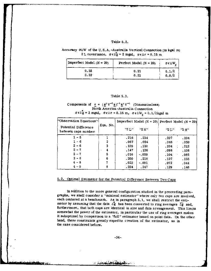
Table 5.2.

Accuracy a4W of the U.S.A. -Australia Vertical Connection (in kgal m)2Lcovariance, ac4= 2mgal, ac7r=0.15m

Imperfect Model (N = 20) Perfect Model (N = 20) a Wt

0.32 0.21 0. lifL0.32 0.21 0.0/1

Table 5.3.

Components of v = (aT V-1 a) - aTV -' (Dimensionless)

North America-Australia Connectionac4=2mgal, ac~r=0.15m, aEAW,=0.1/1kgalim

"Observation Equations" Imperfect Model (N = 20) Perfect Model (N = 20'

Potential Difference Eqn. No.between caps number

1-5 1 .216 .234 .207 .2041 - 6 2 .067 .054 .048 .0502 -6 3 .109 .130 .204 .2122 -7 4 .147 .126 .098 .1083 - 7 5 .016 -.059 .104 .0853 - 8 6 .200 .218 .137 .1554 - 8 7 .022 -.001 .072 .0444 -9 8 .224 .247 .129 .140

5.2. Optimal Estimator for the Potential Difference Between Two Caps

In addition to the more general configuration studied in the preceeding para-graphs, we shall consider a "minimal estimator" where only two caps are involved,each centered at a benchmark. As in paragraph 5. 1, we shall restrict the esti-mator by assuming that the data L* has been converted to ring averages r and,furthermore, that both caps are identical in size and data arrangement. This limitssomewhat the power of the estimator, in particular the use of ring averages makesit suboptimal by comparison to a "full" estimator based on point data. On the otherhand, these constraints greatly expedite creation of the estimator, as inthe case considered before.

-34-

bu#4 n

The objective of the estimator

N Nr.

AT(P, P.) -I'd = fa 1 g,1(l) - fAgj(2) (5.1)I---=12

is to minimize the global mean square of the prediction error:

MfE~T(1 ,P) M = ( M(T(P,, P2 ) - (&'-1 2 d))2 (5.2)

Because both caps are identical, and the average is isotropic (function of sphericaldistance and radial distances only) then, if both caps are on the same sphere, theoptimal weights for each are the same:

1 2 = - or fl1 = f, = f, i=1,2,...,Nr

Accordingly,

Nt

M re AT(P 1 , P2 )' " = M[(T(P) - T(P1) - ;( fi"g1(l) - 'gl(2)) )2 3

= M(T(P) - T(Pa) -f (d _)0)(T(PI) T(Pa_(rd)) I

TC?(O) -Crr(4,t)+_ (tr),-+r 1 ~1 )+f (C2 1 -C1Z 2+D)f

where C is the same as Cdk in (4.14), and CL I , D, CT1, 1 CT areasin (2.7). Thus,

_MEATI = CTiZ -C,11 + (C- 1. 1 - C.,2+ D)_ = 0 (5.3)

or

f = (Ca zr-C, z +D) - (Cra -Cry) (5.4)

since the data consists in values of Ag rather than Ag, a "correction factor"should be used, as before

A T

_T = ( - 1+0.3 f (5.5)

where l (ag ,... ,A I . Using the type of data grid shown in Figure 4. 1,

-35-

*Oki

extended to a 100 cap, so that the average separation of the stations is 40 kin,assuming the same reference gravity fields and covariance models (2 L and 2 H)used before, 0. 1 m relativel position accuracy (cap centers) and 2 mgal accuracyfor the gravity anomalies, the following global rms of the estimation errors werecalculated for various separations Od between the caps:

Table 5.4.

RMS of Error of Optimally Estimated Potential Difference Between the Centers ofTwo 100 Caps O0 Apart. (Imperfect model to degree and order 20, aC = 2 regal,"2 L" covariance function.)

aAW(kgal m) (0)

0.35 1000.40 20c

0.42 300

(RMS fluctuates between 0.41 and 0.42 kgal m for 30" < 4b, 180".)

If the position errors at each cap center are uncorrelated, and if o" c r is their

rms, then a 4 AW should be corrected as follows: a 4E AW' = /( EAW)2+2(0( r)7 .

It is interesting to compare Table 5.4 to Table 4.2: for VWd > 300 . TM_ CAr'"listed above clearly approaches /2 We TIa where /M[ T is the "single cap"accuracy listed in Table 4.2. This also agrees with the increasing independence of es-timates of T separated by more than a few thousand kilometers, pointed out inparagraph 4.4. Similarly, the values of the optimal "weights" fj converge tothose for a single 10' cap, with increasing W.

5.3. Height Differences Between Inaccessible Points

The technique described in this report, in essence, uses accurate positionfixes and a good gravity field model to obtain an estimate of the potential differencebetween points, estimate that is then refined using data from the neighborhood ofeach point (gravity anomalies and levelling) to add high frequency information notcontained in the model. So far we have assumed a good local coverage, easilyaccessible gravity stations and, generally, a most cooperative disposition fromboth Nature and men towards our project. If either, or both, were lacking, wewould be left with the field model, plus some data in the perifery of the region ofinterest to refine the former, and perhaps not even a high accuracy relativeposition fix at each cap center. Through collocation, external data can be incor-porated Into the adjustment, though not as efficiently as in the scheme discussed

The relevant error here is that in the measured difference of geocentric distances.

-36-

, .. -•

in paragraph 4.1. As the data Is far from the point of interest, it is important touse Information rich in long wavelengths signal. One possibility, if the inacces-sible area is not extremely far from the sea, is the mean sea surface derived fromsatellite altimetry, regarded as a quasi-geoid with 1.5 m global rms of "noise"due to dynamic effects. Altimetry could be used on land as well, to provide fixesin radial position for the "cap centers". The surface of an inland sea or lakewould be ideal as a target; other areas where consistent ellipsoidal heights couldbe obtained (i.e., independent of seasonal effects), such as salt-flats in desertareas, etc., could be used if systematic errors due to surface reflectivity weresufficiently understood. With very accurate gravity field models and continuoustracking of the altimeter satellite by another craft in a higher orbit it should bepossible, eventually, to obtain computed orbits good to 0.1 m (rms), which, addedto another 0.1 m (rms) error for the altimeter itself, would amount to near 0.15m (rms) error in the ellipsoidal height fixes, or about 0.2 m relative geocentricheight -ccuracy between benchmarks which would propagate as a 0.2 kgal m errorin potential difference. Gravity field models have been improving at a fast ratein recent years; new and better tracking systems are being developed; full

coverage of altimetry data over the oceans is now available from the Geos-3 andSeasat-l spacecrafts. These are three encouraging signs that, in the comingdecade, there will be enough information to model the field up to degree 180 witha global residual rms of about 1 kgal m for the disturbing potential. Then, verticalconnections good to at least /2 x 1 + (0.2)V - 1.5 kgal m should become feasible.This is the same as the theoretical global accuracy of a system based on tidegauges: it should be much the same as having "tide gauges" inland.

5.4. Some Questions Regarding Accuracy Estimates

The accuracies listed in the various tables of this section depend, mostly,on the applicability of the theory of collocation to the real world. In particular,there are some aspects of collocation open to criticism that deserve a mentionhere. The first one is the unavoidable use of approximate covarlance functions, asthe true ones cannot be known exactly from finite amounts of data, basically becausethe expansion of the "true" gravity field in harmonic polynomials is infinite. Laurit-zen (1973) has established the impossibility of obtaining the covariance of a randomprocess on a sphere even from a complete data coverage, but it is not very clearwhy the gravity field should be treated as a random process in the first place. Be

as it may, the available information is always going to be incomplete and inaccurate.Otherwise, there wouldn't be much point in using collocation, or any other form ofinterpolation and filtering, as there would be little to learn from it. This is whytwo different empirical covarlance functions were used, 1"2 L" and "2 H", to find

out how sensitive the adjusted potential differences were to the choice of function.The results, as shown in the various tables, were much the same with both.

-37-

... ..~

Second, there is the question of how suitable is the spherical harmonicrepresentation of the gravity field on which a good deal of the theory put forwardhere (as much of modern geodesy) rests. From the work of Petroskaya (1977)and Sjberg (1978), who have proposed mathematical formulations for the fieldboth inside and outside the Earth's surface, we learn that such expansions arenot necessarily sums of solid spherical harmonics. On the other hand, it iswell known that the gravity field of a homogeneous ellipsoid can be expressed interms of such harmonics down to a sphere completely buried in the ellipsoid.The Earth being primarily ellipsoidal, we may expect it to have a field that doesnot behave too differently from that of the ellipsoid. However, there is no reasonto expect that the harmonic series that describes the field exactly outside thebounding sphere does so also inside it and down to the Earth's surface. That itdoes not diverge too strongly is shown by the fact that low frequency models de-rived from satellites provide a fit to surface data that improves as more termsare used. That the model is not too inadequate follows from the usefulness offormulas such as Vening Meinesz' and Stokes', which are based on the assumptionthat the field can be expanded in solid spherical harmonics. But all this supportingevidence shows is that these ideas "work" enough to provide about one meter ac-curacy in computed undulations, seconds of arc in deflections of vertical, a fewmilligals in interpolated gravity. No evidence is available to suggest that theyalso "work" at the level of accuracy (approximately 0. 3 to 0.5 m) expected of themhere. Going back to the homogeneous ellipsoid, it is sufficient to add a most minuteinhomogeneity, in the form of a tiny material sphere at any distance R from theorigin, for the series of the composite body to fail to converge inside the sphereof radius R. The mass of the sphere (and therefore the difference between thepure ellipsoidal and the composite field) can be made as small as desired withoutthe series ever converging again. This makes clear that, at least in some cases,a gravity field with a harmonic series that does not converge down to an internalsphere can be only slightly different (except at some isolated points) from one witha series that does. Krarup (1969) brought attention to this fact, and enquiredwhether this might not be always the case. He concluded that it is, furnishingproof of what he called a "Runge-type theorem", because of similar theorems forelliptical differential equations. Krarup's thesis is that any harmonic field can beapproximated uniformly, together with all its derivatives, by sequences of series ofspherical harmonics that converge to an arbitrarily small sphere centered at theorigin, completely inside a surface (terrain) that separates the region where thefield is harmonic from that where it is not. There are a few restrictions on thenature of this surface, but they are loose enough to ensure an adequate fit to thereal topography. The uniform convergence takes place only down to that surface.Inside, the various approximations may differ increasingly from each other, andhave no limit function. So, a spherical harmonic approximation to the exteriorfield can be quite irregular and "wild" in the interior, and this might be a causefor some concern here. The global rms, or accuracy obtained from (2.11), cor-responds to the average of the square of the errors of all possible predictions madeon the same sphere where the actual estimation point is situated. Such sphere isalways partly inside the solid Earth, because of the equatorial bulge. If we imaginethe covariance functions that we are using as corresponding to some spherical har-monic expansion that fits closely the field outside the terrain, they may also cor-

-38-

TI° -,:

respond to a function that has a markedly different character on that part of thesphere that is buried from that which is out In the open. In other words, thespherical harmonic approximations may not be sufficiently "stationary" for ameaningful application of collocation. It may help to understand this problem

having some method to generate the sequences of convergent series Krarup has

spoken of, in order to visualize their behavior. Such method, to this author'sknowledge, has not been proposed yet.

The real question here is whether collocation, and the use of sphericalharmonics theory, may not be a source of bias in the results. In practice there

may be many sources of bias not treated here, such as systematic errors ingravity measurements, position fixes, etc. The only definitive way of knowing

if such factors can be truly significant is to subject the whole idea to experimen-

tation. If enough determinations of potential differences are carried out using

this technique, at many places around the world, between points already connectedby levelling traverses, then any large systematic discrepancies should becomeapparent. If they do not show up, then the experiments will provide supportingevidence for the use of the idea elsewhere.

6. Conclusions

This report has dealt with the concept of World Vertical Network: a set ofbenchmarks thousands of kilometers apart, the geocentric coordinates of, and thepotential differences between which, are accurately known, so they can be used to

connect separate levelling nets in a world-wide system.

The results of section 5 suggest that, according to theory, it might be possibleto set up this network to a significantly better accuracy than that provided by tidegauges and spirit levelling alone. This could be done by using satellite and terres-trial data together, employing least squares collocation as the main mathematical

tool for combining them.

Two cautionary notes are in order: first, there may be causes of error notconsidered in this study that turn out to be of practical significance: only

actual experience can have the final word on this. Second, the estimates of T,crucial to the ideas in this work, are assumed made from values of 6 measured,

or Interpolated, on spherical surfaces. Collocation can be used, in principle, onmore general (terrain-like) surfaces, but the accuracy is not exactly the sameas with the spherical arrangement of data points. "Common sense" suggests that,

if the terrain is gentle, departing smoothly from the spherical shape, the accuracyshould be much the same, but no evidence for this is given here. Numericalstudies are far more difficult when the data is not on a simple spherical arrange-ment, and probably too expensive for an ordinary research project. Furthermore,

whether on the terrain or on a partially buried sphere, the statistical relevance ofthe accuracies derived from collocation can be questioned on the grounds given

at the end of paragraph (5.4). If this is a real problem, it is in--39-

.A iLA.

herent to all applications of collocation theory to estimation of gravitational

field variables inside the Earth's bounding sphere, and not just to the presentideas. This matter seems to h.ve received little or no attention from workersin this area.

Depending primarily on the quality of the reference gravity field model, theaccuracy of the vertical connections in the network could be between 0. 2 and 0.3kgal m, using the data arrangement described in sections 2 and 5. Such configu-ration has been chosen, mostly, to s implify this study, and is by no means theonly possible one. With more data, including satellite altimetry, we could expecteven better results, so those given here are to be regarded as upper limits to the

ultimate quality of a global network.

The North America-Australia connection studied in section 5 requiresrelatively few data (about 4000 point gravity anomalies to 2 mgal accuracy, 8accurate position fixes and a number of levelling traverses, plus a referencemodel to degree and order 20) and the quality of the measurements are almostentirely within present day limits. The exception, the position fixes, can be ex-pected to become feasible within the coming decade. Much of this data can beobtained and used for other purposes, such as the study of polar motion and Earthrotation in the case of the accurate point coordinates. In this way, by sharing withother scientific enterprises, the establishment of the World Vertical Network couldbe made both cheaper and an integral part of the creation of a World GeodeticSystem for positions and heights.

-40-

References

Anderle, R.J., Geodetic Applications of the NAVSTA R Global PositioningSystem, paper presented at the Second International Symposium on ProblemsRelated to the Redefinition of the North American Geodetic Network, Wash-ington, D.C., April 24-28, 1978.

Balmino, G., Introduction to Least Squares Collocation, In "Approximation Methodsin Geodesy", H. Moritz and H. Siinkel editors, pp. 47-89, Herbert WichmannVerlag, Karlsruhe, 1978.

Cartwright, D. E., and J. Crease, A Comparison of the Geodetic Reference Levelsof England and France by Means of Mean Sea Surface, Proc. Royal Society,A 273, pp. 558-580, 1963.

Christodoulidis, D.C., On the Realization of a 10 cm Relative Oceanic Geoid,Report No. 247, Department of Geodetic Science, The Ohio State University,Columbus, Ohio, 1976.

Colombo, 0. L., Optimal Estimation from Data Regularly Sampled on a Sphere,Report No. 291, Department of Geodetic Science, The Ohio State University,Columbus, Ohio, 1979.

Jekeli, C., An Investigation of Two Models for the Degree Variances of GlobalCovariance Functions, Report No. 275, Department of Geodetic Science, TheOhio State University, Columbus, Ohio, 1978.

Kaula, W. M., Statistical and Harmonic Analysis of Gravity, Technical Report,Army Map Service, Washington, D.C., 1959.

Krakiwsky, E. J., and I. I. Mueller, Systems of Height, Report No. 60, Depart-ment of Geodetic Science, The Ohio State University, Columbus, Ohio, 1965.

Krarup, T., A Contribution to the Mathematical Foundation of Physical Geodesy,Geodaetisk Institut, Copenhagen, Denmark, 1969.

Lauritzen, S. L., The Probabilistic Background of Some Statistical Methods inPhysical Geodesy, Geodaetisk Institut, Copenhagen, Denmark, 1973.

Lelgemann, D., Some Problems Concerned with the Geodetic Use of High Pre-cision Altimeter Data, Report No. 237, Department of Geodetic Science, TheOhio State University, Columbus, 1976.

Lerch, F., S.M. Klosko, et. al., Gravity Model Improvement Using Geos-3Altimetry: GEM 10A and GEM 10B, Goddard Space Flight Center, (NASA),Report X-921-77-246, Greenbelt, Maryland, 1977.

-41-

v

• . ,~

Mather, R.S., C. Rizos and T. Morrison, On the Unification ct Geodetic Levelling

Datums Using Satellite Altimetry, NASA Technical Memorandum 79533, 1978.

Moritz, H., Advanced Least Squares Methods, Report No. 175, Department of

Geodetic Science, The Ohio State University, Columbus, Ohio, 1972.

Petroskaya, M.S., Generalization of Laplace's Expansion to the Earth's Surface,

Bulletin Ggodisique, Vol. 51, pp. 53-62, Paris, 1977.

Rao, C. R., Linear Statistical Inference and its Applications, pp. 71-73, JohnWiley and Sons, New York, 1973.

Rapp, R. H., Results of the Application of Least Squares Collocation to Selected

Geodetic Problems, in "Approximation Methods in Geodesy", pp. 117-157,1978a.

Rapp, R. H., A Global lox 1 Anomaly Field Combining Satellite, Geos-3 Altimeterand Terrestrial Anomaly Data, Report No. 278, Department of Geodetic Science,

The Ohio State University, Columbus, Ohio, 1978b.

Rummel, R., and K. P. Schwarz, On the Nonhomogeineity of the Global CovarianceFunction, Bulletin G6odesique, Vol. 51, pp. 93-103, 1977.

Silverberg, E.C., et. al., An Estimate of the Geodetic Accuracy Attainable with a

Transportable Lunar Laser Station, Bulletin Geodesique, Vol. 50, pp. 331-340,1976.

Sjberg, L., On the Errors of Spherical Harmonic Developments of Gravity at theSurface of the Earth, Report No. 257, Department of Geodetic Science, TheOhio State University, Columbus, Ohio, 1977.

Tengstrom, E., and A. Vogel, Research on Methods for Determining Level Sur-faces of the Earth's Gravity Field, Final Report, Geodetic Institute, UppsalaUniversity, 1965.

-42-

........................- ,.

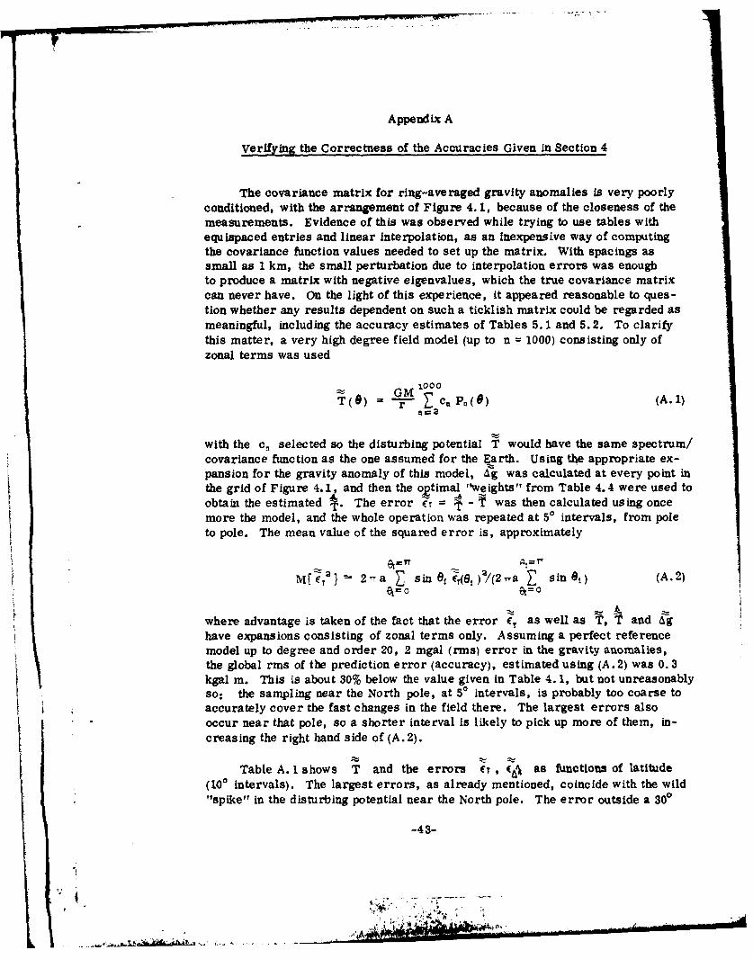
Appendix A

Verifying the Correctness of the Accuracies Given in Section 4

The covariance matrix for ring-averaged gravity anomalies is very poorlyconditioned, with the arrangement of Figure 4. 1, because of the closeness of themeasurements. Evidence of this was observed while trying to use tables withequispaced entries and linear interpolation, as an Inexpensive way of computingthe covariance function values needed to set up the matrix. With spacings assmall as 1 kin, the small perturbation due to interpolation errors was enoughto produce a matrix with negative eigenvalues, which the true covariance matrixcan never have. On the light of this experience, it appeared reasonable to ques-tion whether any results dependent on such a ticklish matrix could be regarded asmeaningful, including the accuracy estimates of Tables 5. 1 and 5.2. To clarifythis matter, a very high degree field model (up to n = 1000) consisting only ofzonal terms was used

G G 000TGM)c= P. (a) (A. 1)

with the c, selected so the disturbing potential T would have the same spectrum/covariance function as the one assumed for the Earth. Using the appropriate ex-pansion for the gravity anomaly of this model, &g was calculated at every point inthe grid of Figure 4.1, and then the o~timal "weights" from Table 4.4 were used to

obtain the estimated t. The error CT = 6 - T was then calculated using oncemore the model, and the whole operation was repeated at 50 intervals, from poleto pole. The mean value of the squared error is, approximately

MrEC_,' 2,7a Zsin 81 C48,)Y2ira sin 8 t) (A. 2)G%=o

where advantage is taken of the fact that the error f as well as t, and Aghave expansions consisting of zonal terms only. Assuming a perfect referencemodel up to degree and order 20, 2 regal (rms) error in the gravity anomalies,the global rms of the prediction error (accuracy), estimated using (A. 2) was 0.3kgal m. This is about 30% below the value given in Table 4. 1, but not unreasonablyso: the sampling near the North pole, at 5 intervals, is probably too coarse toaccurately cover the fast changes in the field there. The largest errors alsooccur near that pole, so a shorter interval is likely to pick up more of them, in-creasing the right hand side of (A. 2).

Table A. 1 shows T and the errors T , 0(,p as functions of latitude(100 intervals). The largest errors, as already mentioned, coincide with the wild"spike" in the disturbing potential near the North pole. The error outside a 300

-43-

polar cap is almost everywhere less than the global rms. This suggests that theworst predictions can occur where the field has large and fast variations. Thepercentage of error in the predicted value, however, is about 10% at the pole, sothe relative goodness of the prediction is not particularly bad there. But we areinterested in the absolute value of the error, so the pole is clearly a bad place,in this "artificial planet", for making estimates. Table A. 1 shows that the be-havior of Ag closely resembles that of . In this particular case, the predic-tion of T is bad where that of Yg is bad,' and vice versa, and this could beused as a practical criterion for selecting the locations of estimation points.Predicting Ag from gravimetry in a "candidate" region, at points in that regionwhere 4g is already known from accurate measurements, we could comparethe actual error in these estimates to the theoretical accuracy of expression(2. 11). If the actual errors are close to their theoretical rms, the region isacceptable, and we can proceed to set up a cap like that one in Figure 4. 1; if theerrors are consistently larger, the region should be rejected.

Other points to consider when selecting a place for a cap are: lack of sig-nificant bodies of free water, because gravity cannot be measured as accuratelyon water as on land; smooth topography (with most places easily accessible) topermit accurate levelling and good coverage with gravity stations.

1g is estimated here using a "4 points' cross" pattern centered at the prediction

point. The "arms" are 20 km wide.

-44-

4 - ,. -. , ",• . . . , . .;i~,,W , .

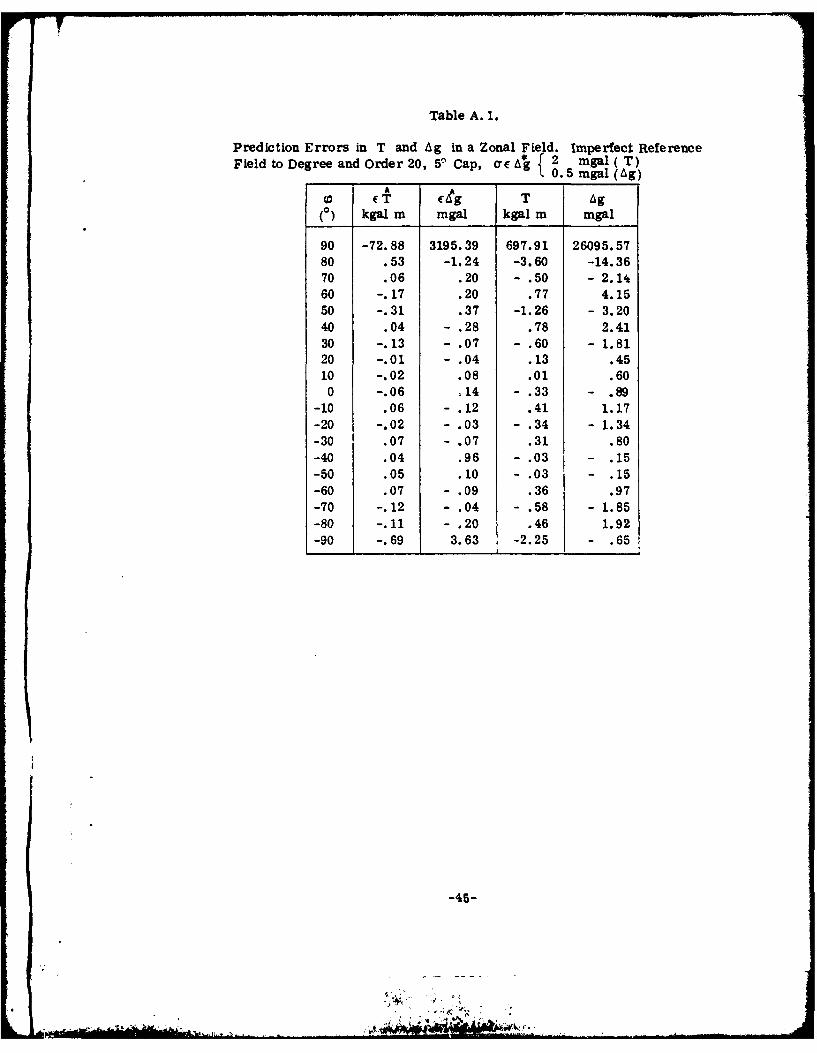
Table A. 1.

Prediction Errors in T and Ag in a Zonal Field. Imperfect ReferenceField to Degree and Order 20, 5 Cap, ac A* 2 mgal ( T)

S0. mgal (Ag)A

cT ceg T Ag(0) kgal m mgal kgal m mgal

90 -72.88 3195.39 697.91 26095.5780 .53 -1.24 -3.60 -14.3670 .06 .20 - .50 - 2.1460 -.17 .20 .77 4.1550 -. 31 .37 -1.26 - 3.2040 .04 - .28 .78 2.4130 -. 13 - .07 - .60 -1.8120 -. 01 - .04 .13 .45

10 -. 02 .08 .01 .600 -. 06 . 14 - .33 - .89

-10 .06 - .12 .41 1.17-20 -. 02 - .03 - .34 -1.34-30 .07 - .07 .31 .80-40 .04 .96 - .03 - .15-50 .05 .10 - .03 - .15-60 .07 - .09 .36 .97-70 -.12 - .04 - .58 -1.85

-80 -. 11 - .20 .46 1.92-90 -. 69 3.63 -2.25 - .65

-45-

Appendix B

This Appendix contains listings of parts of the software developed for thisproject, and sample output. First there is a listing of "RINGS", a program thatobtains the optimal components, or weights, of the estimator vector f (expression(2.6)). This program sets up a grid of the kind shown in Figure 4.1 for a cap ofsize CAPSIZ (in degrees). The number of rings in the cap is NP, so, with theorigin, there are NP+1 weights to be found. The listing clearly shows the variousconstants used. REGPAR is a "regularization" parameter, chosen here very small.This number is added to the main diagonal of the normal matrix C,, + D to improvethe stability of the solution. NMOD is the maximum degree and order in the refer-ence model. To change it into a "perfect" model, a statement setting all values inDVAR to zero is added before the statement "55 CONTINUE". GNOISE is the stan-dard deviation of At in mgals. The solution is obtained using the conjugate gradi-ents procedure in subroutine CGRADS. The maximum number of iterations allowed,ITERMX, is the number of unknown (NP + 1) plus ten. However, if the improvementin the rms of the solution from iteration to iteration is less than one part in a million,the procedure terminates then. Program RINGS sets up the normal matrix takingadvantage, as far as possible, of the various symmetries in the grid. After thesolution has been found, it multiplies both rms and weights by the correction factor

NP+ I1 + k1 Z fi (paragraph (4.2)), and it also multiplies (C,, + D)f reconstructedright hand sides of normals, to compare them with the original rms's, showingwhether the conjugate gradient procedure has, in fact, converged. The listing ofRINGS is complemented by those of the subroutines it calls: CGRADS, MATVEC,LEGPOL, COVAR, and function F.

A At

Finally, subroutine RINCOV, used to determine the covariance M E T (Pi)E T(PfIbetween prediction errors, based on (4.14) and the repeated use of expression (4.17),is listed as well. The main array and variables are given the same names as inRINGS and associated subroutines, with the exception of the optimal weights vector,here called "F".

-46-

se.;

C4.0

C4 9C4

Cd 00 w ; C

lad- N

0% CC If

V .. in -aft '@t.t-ccO

03-- 0o4 co C13.

p 4 44 16.0

'@04.4 - 4

09 0!D 006 C04.

0 Mlo~l~mtII I-

wo 03a aCc*S,

94 e~

* -~ O-47-

it-

U.

S.

00

*1$

04o

0®

'0O

..

-I.-

i ...... . ... ... . . ........ .... .. , ,, .. . ._ .. ._

.. c

0 E0

-;a-

- ~ .%O

NEU

21ci efMclc

[-PC \) 0 ,oC 00u" a 0"Dt

o~~ man"..~ hNo- 9 0 - - N1

0040 8000

00O 0004DO40 :000000:0 OOM000 -a :

-h. U~\ O@ ~ -049-t~~s

CIN

.cc

iijaI .-

II + I\ IC i0 as 40 II- - i: 4

* 1m

C3an~! T a;; otA CS AC00 t ! - N

* u 04 C, :96 Nl NM0i l

ac U

a li! R- * i fj Q . it

o------- ~I0-W.~Wiefif II 1 NH~i

* .~ ~;; -50 a

l - gig

82 b4 P0 NP*

*^ 80". -

0D 8c I .0-09*H I- 1421

64 t 1

*mee

SH M0 - 0 :3 000 006666 *so.- ~ bhI1

I ;

k e!ta

.11" \j a

. *

10 4ar Q

!-52-.__ , o -. o(, .a, 8 @ , + -,-

eal. .. .. ~ . ..

16

00

40

I, ;

- 0:

* 91"

0 '- i 11111 i i a irif% E- NN grrt -t-s0.20

o" - - - -- - -§ - --

*00 0 0000 0B 00 00000

4'--.-~ a 53-

.I

r - _ Ui,-,,( . • 9= .1® m I . ! " ".t

q ,*

WID

- m -U """, E

" - - tIRg @

-bro!... ass s iazgCs~sziw

-54-

- .. ' -; w -

: .. . ; 'a °m: II - -' i: L mfl "' , . . .. ... ... .. .. ,l ~,a

In

00

r.. CO

*cch

-55

4.

l imh~ 656-

IIis23l.

Irj~~ -.F

*e99

U~ -ai 4

40!N +-CIr 10 40 8 310

Goa HA MN -qr

C. *i m-i -

:10 000600 :Go Q: oo

-57,

2

U4t

o 0

S. .

I * .* *

-58-

*eee~e*wee*

ti

_+43 SOO - Q Q

~M 0

~ I -

%9 % "

-59-S- - --

eeoce.:::

SS

I!* N

Mp ~ NI.

Eq* NN. N

N

* Eq_ U

SE

#4'.,N

U-

M mi N~

~I..; ~9 ~

-; ~eq *

6

I -

U

b-60-

0

04

-'t 0o ~ e000

*i A

cl 0 1ri*

lK on

m NT ci:*

OS- * c19 u 96 - -- -- - - - *OC04fi gas*

4411 444. .. . . . .

.- C*-d%% jAN co 0 *

2>> * *

0 r. u * u

COM -4 -0 -0 ;;j(]klcc *V40 00:00 *0

0 0 co*ecmco0 coes o

010ccmnnoaa

94 44 9^*x 1

*e N

* *m* on-

010 * *

44 44* m 9

04 44 -4

01 * i riwr ir ir

00 a44 * *

Mo M* :: SHO

44 -- 62-

00 00

IICA

-t

40 Ca No. .41

3 0 s via-

I* k I, Co k

U *.2~ ~b.mm U ~..-63- m