Embed Size (px)
Citation preview

Lecture 13. Inverse Laplace Transformation
• Inverse Laplace TransformP l i l• Polynomials
• Roots, zeros and poles• Complex numbersp• Step & Delta functions
1

Solving Differential Equationsg q
• Example: For zero initial conditions, solve
)(4)(30)(11)(2
2
tutydt
tyddt
tyd=++
• Laplace transform approach automatically includes initial conditions in the solution
dtdt
in the solution
)0()()( yssdt
tyd−=⎥⎦
⎤⎢⎣⎡ YL
)0(')0()()( 22
2
yysssdt
tyd−−=⎥
⎦
⎤⎢⎣
⎡⎦⎣
YL
2

Solving Differential Equations (cont’d)g q ( )
• Laplace transform of the equation
ssYyssYysysYs 4)(30)0(11)(11)0(')0()(2 =+−+−−
)3011(4)11)0('()0()( 2
2
+++++
=sss
ysyssY)3011( ++ sss
Easy to solve the differential equation in Laplace space,but needs to transform the solution to real space!p
Inverse Laplace Transform3
p
Inverse Laplace Transformp
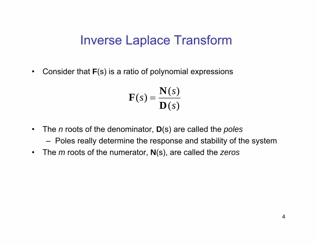
• Consider that F(s) is a ratio of polynomial expressions
)()()(
sss
DNF =
• The n roots of the denominator, D(s) are called the polesP l ll d t i th d t bilit f th t
)(sD
– Poles really determine the response and stability of the system• The m roots of the numerator, N(s), are called the zeros
4

Inverse Laplace Transformp
• We will use partial fractions expansion with the method p pof residues to determine the inverse Laplace transform
• Three possible cases (need proper rational, i.e., n>m)1. simple poles (real and unequal)2. simple complex roots (conjugate pair)2. simple complex roots (conjugate pair)3. repeated roots of same value
5

1. Simple Polesp
• Simple poles are placed in a partial fractions expansion
( ) ( )( )( ) ( ) n
n
n
m
psK
psK
psK
pspspszszsK
s+
+++
++
=+++
++= K
L
L
2
2
1
1
21
10)(F
• The constants, Ki, can be found from (use method of residues)
( )( ) ( ) nn pppppp 2121
• Finally, tabulated Laplace transform pairs are used to invert ipsii spsK
−=+= )()( F
y, p pexpression, but this is a nice form since the solution is
tptptp neKeKeKtf −−− +++= L2121)(
6
n eKeKeKtf +++ 21)(

2. Complex Conjugate Polesp j g
• Complex poles result in a Laplace transform of the form
+++
−∠+
−+
∠=+
+++
−+=
)()()()()( 11
*11
βαθ
βαθ
βαβα jsK
jsK
jsK
jsK
s LF
• The K1 can be found using the same method as for simple poles
βα sjsK −+= )()(1 FWARNING: the "positive" pole of the form –α+jβ MUST be the one that
is used
βαβα
jssjsK
+−=+ )()(1 F
• The corresponding time domain function is
( ) L++= − θβα teKtf t cos2)( 1
7
( )++θβ teKtf cos2)( 1
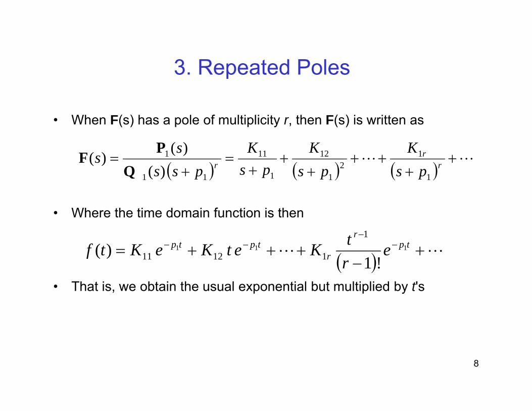
3. Repeated Polesp
• When F(s) has a pole of multiplicity r, then F(s) is written as
( ) ( ) ( )LL +
+++
++
+=
+= r
rr ps
Kps
Kps
Kpss
ss1
12
1
12
1
11
11
1
)()()(
QPF
• Where the time domain function is then
( ) ( ) ( )1111
1
Th t i bt i th l ti l b t lti li d b t'
( ) LL +−
+++= −−
−− tpr
rtptp e
rtKetKeKtf 111
!1)(
1
11211
• That is, we obtain the usual exponential but multiplied by t's
8

3. Repeated Poles (cont’d.)p ( )
• The K1j terms are evaluated from1j
( ) ( )[ ])(!
111
ps
rjr
jr
j spsdsd
jrK
−=−
−
+−
= F
• This actually simplifies nicely until you reach s³ terms, that is for a double root (s+p1)²
( )1ps −=
that is for a double root (s+p1)²
( ) ( )[ ]1
)()( 2111
2112 ps
spsdsdKspsK
−=+=+= FF
• Thus K12 is found just like for simple roots
11 ps
p ds −=
9
12 j p• Note this reverse order of solving for the K values

The “Finger” Methodg
• Let’s suppose we want to find the inverse Laplace pp ptransform of
)3)(2()1(5)(++
+=
sssssF
• We’ll use the “finger” method which is an easy way of visualizing the method of residues for the case of simple
)3)(2( ++ sss
visualizing the method of residues for the case of simple roots (non-repeated)
• We note immediately that the poles ares1 = 0 ; s2 = –2 ; s3 = –3
10

The Finger Method (cont’d)g ( )
• For each pole (root), we will write down the function F(s) and put our finger over the term that caused that particular root, and then substitute that pole (root) value into every other occurrence of ‘s’ in F(s); let’s start with s1=0
65
)3)(2()1(5
)30)(20)(()10(5
)3)(2()1(5)( ==
+=
+=
ssF
Thi l i h ffi i f h i f
6)3)(2()30)(20)(()3)(2()(
++++ ssss
• This result gives us the constant coefficient for the inverse transform of that pole; here: e–0·t
11

The Finger Method (cont’d)g ( )
• Let’s ‘finger’ the 2nd and 3rd poles (s2 & s3)
25
)1)(2()1(5
)32)(2)(2()12(5
)3)(2()1(5)( =
−−
=+−+−
+−=
+++
=ssss
ssF
310
)1)(3()2(5
)3)(23)(3()13(5
)3)(2()1(5)(
))(())()(())((−
=−−
−=
++−−+−
=++
+=
ssssssF
• They have inverses of e–2·t and e–3·t
• The final answer is then
tt eetf 32
310
25
65)( −− −+=
12
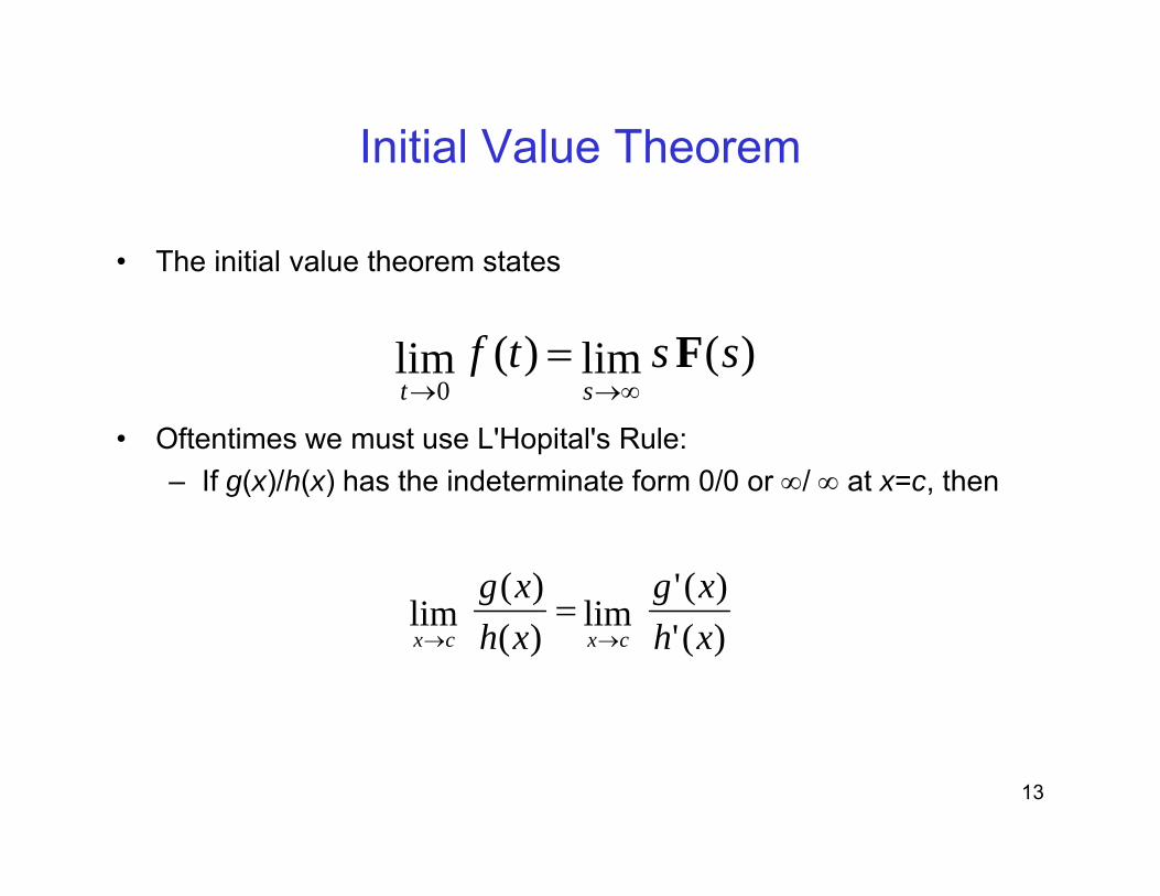
Initial Value Theorem
• The initial value theorem states
)(lim)(lim0
s s tfst
F∞→→
=
• Oftentimes we must use L'Hopital's Rule:– If g(x)/h(x) has the indeterminate form 0/0 or ∞/ ∞ at x=c, then
0 st ∞→→
)('lim
)(lim
xgxg=
)('lim)(lim xh
xh
cxcx →→
13

Final Value Theorem
• The final value theorem states
)(lim)(lim s s tf 0st
F→∞→
=
• The initial and final value theorems are useful for determining initial and steady state conditions respectively for transient circuitand steady-state conditions, respectively, for transient circuit solutions when we don’t need the entire time domain answer and we don’t want to perform the inverse Laplace transform
14
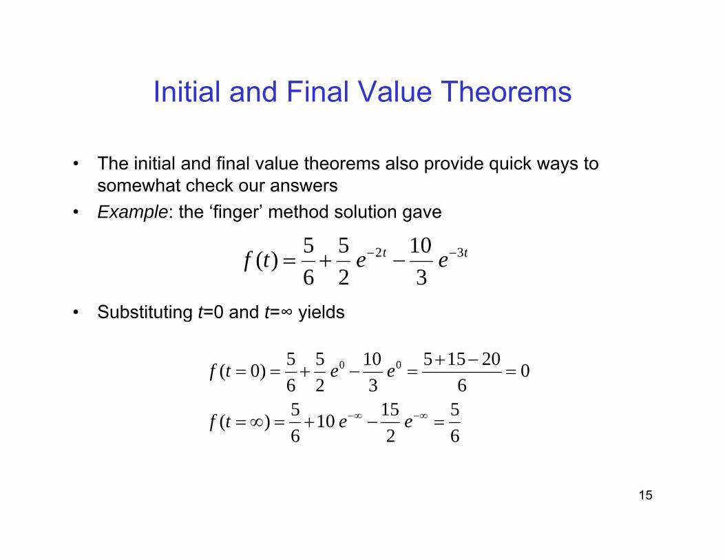
Initial and Final Value Theorems
• The initial and final value theorems also provide quick ways to somewhat check our answers
• Example: the ‘finger’ method solution gave
1055
• Substituting t=0 and t=∞ yields
tt eetf 32
310
25
65)( −− −+=
Substituting t 0 and t yields
06
201553
1025
65)0( 00 =
−+=−+== eetf
65
21510
65)(
6326
=−+=∞= ∞−∞− eetf
15

Initial and Final Value Theorems
• What would initial and final value theorems find?• First, try the initial value theorem (L'Hopital's too)
)3)(2()1(5
lim)(lim)0( ∞=
+++
==ss s f F
0552
5lim65
)1(5lim)0(
)3)(2(
2 =∞
=+
=++
+=
∞++
∞→∞→
∞→∞→
ssss
f
ss
sdsd
dsd
s
ss
• Next, employ final value theorem5)1(5)1(5
lim)(lim)( ==+
==∞sssf F
• This gives us confidence with our earlier answer
6)3)(2()3)(2(lim)(lim)(00
==++
==∞→→ ss
ss fss
F
16

Class Examplesp
• Find Inverse Laplace Transforms of
)1()( 2+=
sssY
84)(
)1(
2=
+ss
s
Z84
)( 2 ++ ss
17


