Embed Size (px)
Citation preview

EECC722 - ShaabanEECC722 - Shaaban#1 Lec # 1 Fall 2003 9-8-2003
Advanced Computer ArchitectureAdvanced Computer Architecture Course Goal:Understanding important emerging design techniques, machine structures, technology factors, evaluation methods that willdetermine the form of high-performance programmable processors andcomputing systems in 21st Century.
Important Factors:• Driving Force: Applications with diverse and increased computational demands even in mainstream
computing (multimedia etc.)• Techniques must be developed to overcome the major limitations of current computing systems to
meet such demands:– ILP limitations, Memory latency, IO performance.– Increased branch penalty/other stalls in deeply pipelined CPUs.– General-purpose processors as only homogeneous system computing resource.
• Enabling Technology for many possible solutions: – Increased density of VLSI logic (one billion transistors in 2004?)– Enables a high-level of system-level integration.

EECC722 - ShaabanEECC722 - Shaaban#2 Lec # 1 Fall 2003 9-8-2003
Course TopicsTopics we will cover include:• Overcoming inherent ILP limitations by exploiting Thread-level Parallelism (TLP):
– Support for Simultaneous Multithreading (SMT). • Alpha EV8. Intel P4 Xeon (aka Hyper-Threading), IBM Power5.
– Introduction to Multiprocessors:• Chip Multiprocessors (CMPs): The Hydra Project. IBM Power4, 5
• Memory Latency Reduction:
– Conventional & Block-based Trace Cache (Intel P4).
• Advanced Branch Prediction Techniques.
• Towards micro heterogeneous computing systems:– Vector processing. Vector Intelligent RAM (VIRAM).– Digital Signal Processing (DSP) & Media Architectures & Processors.– Re-Configurable Computing and Processors.
• Virtual Memory Implementation Issues.
• High Performance Storage: Redundant Arrays of Disks (RAID).

EECC722 - ShaabanEECC722 - Shaaban#3 Lec # 1 Fall 2003 9-8-2003
Computer System ComponentsComputer System Components
SDRAMPC100/PC133100-133MHZ64-128 bits wide2-way inteleaved~ 900 MBYTES/SEC
Double DateRate (DDR) SDRAMPC3200400MHZ (effective 200x2)64-128 bits wide4-way interleaved~3.2 GBYTES/SEC(second half 2002)
RAMbus DRAM (RDRAM)PC800, PC1060 400-533MHZ (DDR)16-32 bits wide channel~ 1.6 - 3.2 GBYTES/SEC ( per channel)
CPU
CachesSystem Bus
I/O Devices:
Memory
Controllers
adapters
DisksDisplaysKeyboards
Networks
NICs
I/O BusesMemoryController
Examples: Alpha, AMD K7: EV6, 400MHZ Intel PII, PIII: GTL+ 133MHZ Intel P4 800MHZ
Example: PCI-X 133MHZ PCI, 33-66MHZ 32-64 bits wide 133-1024 MBYTES/SEC
1000MHZ - 3 GHZ (a multiple of system bus speed)Pipelined ( 7 -21 stages )Superscalar (max ~ 4 instructions/cycle) single-threadedDynamically-Scheduled or VLIWDynamic and static branch prediction
L1
L2 L3
Memory Bus
Support for one or more CPUs
Fast EthernetGigabit EthernetATM, Token Ring ..
NorthBridge
SouthBridge
Chipset

EECC722 - ShaabanEECC722 - Shaaban#4 Lec # 1 Fall 2003 9-8-2003
Computer System ComponentsComputer System Components
CPU
CachesSystem Bus
I/O Devices:
Memory
Controllers
adapters
Disks (RAID)DisplaysKeyboards
Networks
NICs
I/O BusesMemoryController
L1
L2 L3
Memory Bus
Conventional & Block-based Trace Cache.
Integrate MemoryController & a portionof main memory with CPU: Intelligent RAM
Integrated memory Controller: AMD Opetron
IBM Power5
Memory Latency Reduction:
Enhanced CPU Performance & Capabilities:
• Support for Simultaneous Multithreading (SMT): Alpha EV8.• VLIW & intelligent compiler techniques: Intel/HP EPIC IA-64.• More Advanced Branch Prediction Techniques.• Chip Multiprocessors (CMPs): The Hydra Project. IBM Power 4,5• Vector processing capability: Vector Intelligent RAM (VIRAM). Or Multimedia ISA extension.• Digital Signal Processing (DSP) capability in system.• Re-Configurable Computing hardware capability in system.
SMTCMP
NorthBridge
SouthBridge
Chipset

EECC722 - ShaabanEECC722 - Shaaban#5 Lec # 1 Fall 2003 9-8-2003
EECC551 ReviewEECC551 Review• Recent Trends in Computer Design.Recent Trends in Computer Design.
• A Hierarchy of Computer Design.A Hierarchy of Computer Design.
• Computer Architecture’s Changing Definition.Computer Architecture’s Changing Definition.
• Computer Performance Measures.Computer Performance Measures.
• Instruction Pipelining.Instruction Pipelining.
• Branch Prediction.Branch Prediction.
• Instruction-Level Parallelism (ILP).Instruction-Level Parallelism (ILP).
• Loop-Level Parallelism (LLP).Loop-Level Parallelism (LLP).
• Dynamic Pipeline Scheduling.Dynamic Pipeline Scheduling.
• Multiple Instruction Issue (CPI < 1): Superscalar vs. VLIWMultiple Instruction Issue (CPI < 1): Superscalar vs. VLIW
• Dynamic Hardware-Based SpeculationDynamic Hardware-Based Speculation• Cache Design & Performance.Cache Design & Performance.

EECC722 - ShaabanEECC722 - Shaaban#6 Lec # 1 Fall 2003 9-8-2003
Recent Trends in Computer DesignRecent Trends in Computer Design• The cost/performance ratio of computing systems have seen a
steady decline due to advances in:
– Integrated circuit technology: decreasing feature size, • Clock rate improves roughly proportional to improvement in • Number of transistors improves proportional to (or faster).
– Architectural improvements in CPU design.
• Microprocessor systems directly reflect IC improvement in terms of a yearly 35 to 55% improvement in performance.
• Assembly language has been mostly eliminated and replaced by other alternatives such as C or C++
• Standard operating Systems (UNIX, NT) lowered the cost of introducing new architectures.
• Emergence of RISC architectures and RISC-core architectures.
• Adoption of quantitative approaches to computer design based on empirical performance observations.

EECC722 - ShaabanEECC722 - Shaaban#7 Lec # 1 Fall 2003 9-8-2003
Microprocessor Architecture TrendsMicroprocessor Architecture Trends
C IS C M ac h i n e sins truc tio ns take var iable t im e s to c o m ple te
R IS C M ac h i n e s ( m i c r o c o d e )s im ple ins truc tio ns , o ptim ize d fo r spe e d
R IS C M ac h i n e s ( p i p e l i n e d )s am e individual ins truc tio n late nc y
gre ate r thro ughput thro ugh ins truc tio n "o ve r lap"
S u p e r s c a l ar P r o c e s s o r sm ultiple ins truc tio ns e xe c uting s im ultane o us ly
M u l t i t h r e ad e d P r o c e s s o r saddit io nal H W re so urc e s ( re gs , P C , SP )e ac h c o nte xt ge ts pro c e s so r fo r x c yc le s
V L IW"Supe r ins truc tio ns " gro upe d to ge the r
de c re ase d H W c o ntro l c o m ple xity
S i n g l e C h i p M u l t i p r o c e s s o r sduplic ate e ntire pro c e s so rs
( te c h so o n due to M o o re 's Law)
S IM U L TA N E O U S M U L TITH R E A D IN Gm ultiple H W c o nte xts ( re gs , P C , SP )e ac h c yc le , any c o nte xt m ay e xe c ute
CMPs
(SMT)
SMT/CMPs (e.g. IBM Power5 in 2004)

EECC722 - ShaabanEECC722 - Shaaban#8 Lec # 1 Fall 2003 9-8-2003
1988 Computer Food Chain1988 Computer Food Chain
PCWork-stationMini-
computer
Mainframe
Mini-supercomputer
Supercomputer
Massively Parallel Processors

EECC722 - ShaabanEECC722 - Shaaban#9 Lec # 1 Fall 2003 9-8-2003
1997- Computer Food Chain1997- Computer Food Chain
PCWork-station
Mainframe
Supercomputer
Mini-supercomputerMassively Parallel Processors
Mini-computer
ServerPDA
Clusters

EECC722 - ShaabanEECC722 - Shaaban#10 Lec # 1 Fall 2003 9-8-2003
Processor Performance TrendsProcessor Performance Trends
Microprocessors
Minicomputers
Mainframes
Supercomputers
Year
0.1
1
10
100
1000
1965 1970 1975 1980 1985 1990 1995 2000
Mass-produced microprocessors a cost-effective high-performance replacement for custom-designed mainframe/minicomputer CPUs

EECC722 - ShaabanEECC722 - Shaaban#11 Lec # 1 Fall 2003 9-8-2003
Microprocessor Performance Microprocessor Performance 1987-971987-97
0
200
400
600
800
1000
1200
87 88 89 90 91 92 93 94 95 96 97
DEC Alpha 21264/600
DEC Alpha 5/500
DEC Alpha 5/300
DEC Alpha 4/266IBM POWER 100
DEC AXP/500
HP 9000/750
Sun-4/
260
IBMRS/
6000
MIPS M/
120
MIPS M
2000
Integer SPEC92 PerformanceInteger SPEC92 Performance

EECC722 - ShaabanEECC722 - Shaaban#12 Lec # 1 Fall 2003 9-8-2003
Microprocessor Frequency TrendMicroprocessor Frequency Trend
386486
Pentium(R)
Pentium Pro(R)
Pentium(R) II
MPC750604+604
601, 603
21264S
2126421164A
2116421064A
21066
10
100
1,000
10,000
19
87
19
89
19
91
19
93
19
95
19
97
19
99
20
01
20
03
20
05
Mh
z
1
10
100
Ga
te D
ela
ys
/ Clo
ck
Intel
IBM Power PC
DEC
Gate delays/clock
Processor freq scales by 2X per
generation
Frequency doubles each generation Number of gates/clock reduce by 25%
Result:Deeper PipelinesLonger stallsHigher CPI

EECC722 - ShaabanEECC722 - Shaaban#13 Lec # 1 Fall 2003 9-8-2003
Microprocessor Transistor Microprocessor Transistor Count Growth RateCount Growth Rate
Year
Tra
nsis
tors
1000
10000
100000
1000000
10000000
100000000
1970 1975 1980 1985 1990 1995 2000
i80386
i4004
i8080
Pentium
i80486
i80286
i8086 Moore’s Law:Moore’s Law:2X transistors/ChipEvery 1.5 yearsStill valid possibly until 2010
Alpha 21264: 15 millionPentium Pro: 5.5 millionPowerPC 620: 6.9 millionAlpha 21164: 9.3 millionSparc Ultra: 5.2 million
Moore’s Law
One billion in 2004?

EECC722 - ShaabanEECC722 - Shaaban#14 Lec # 1 Fall 2003 9-8-2003
Increase of Capacity of VLSI Dynamic RAM ChipsIncrease of Capacity of VLSI Dynamic RAM Chips
size
Year
Bit
s
1000
10000
100000
1000000
10000000
100000000
1000000000
1970 1975 1980 1985 1990 1995 2000
year size(Megabit)
1980 0.0625
1983 0.25
1986 1
1989 4
1992 16
1996 64
1999 256
2000 1024
1.55X/yr, or doubling every 1.6 years

EECC722 - ShaabanEECC722 - Shaaban#15 Lec # 1 Fall 2003 9-8-2003
Recent Technology Trends Recent Technology Trends (Summary) (Summary)
Capacity Speed (latency)
Logic 2x in 3 years 2x in 3 years
DRAM 4x in 3 years 2x in 10 years
Disk 4x in 3 years 2x in 10 yearsResult: Widening gap between CPU performance & memory/IO performance

EECC722 - ShaabanEECC722 - Shaaban#16 Lec # 1 Fall 2003 9-8-2003
Computer Technology Trends:Computer Technology Trends: Evolutionary but Rapid ChangeEvolutionary but Rapid Change
• Processor:– 2X in speed every 1.5 years; 100X performance in last decade.
• Memory:– DRAM capacity: > 2x every 1.5 years; 1000X size in last decade.– Cost per bit: Improves about 25% per year.
• Disk:– Capacity: > 2X in size every 1.5 years.– Cost per bit: Improves about 60% per year.– 200X size in last decade.– Only 10% performance improvement per year, due to mechanical limitations.
• Expected State-of-the-art PC by end of year 2003 :– Processor clock speed: > 3400 MegaHertz (3.2 GigaHertz)– Memory capacity: > 4000 MegaByte (2 GigaBytes)– Disk capacity: > 300 GigaBytes (0.3 TeraBytes)

EECC722 - ShaabanEECC722 - Shaaban#17 Lec # 1 Fall 2003 9-8-2003
A Hierarchy of Computer DesignA Hierarchy of Computer DesignLevel Name Modules Primitives Descriptive Media
1 Electronics Gates, FF’s Transistors, Resistors, etc. Circuit Diagrams
2 Logic Registers, ALU’s ... Gates, FF’s …. Logic Diagrams
3 Organization Processors, Memories Registers, ALU’s … Register Transfer
Notation (RTN)
4 Microprogramming Assembly Language Microinstructions Microprogram
5 Assembly language OS Routines Assembly language Assembly Language
programming Instructions Programs
6 Procedural Applications OS Routines High-level Language
Programming Drivers .. High-level Languages Programs
7 Application Systems Procedural Constructs Problem-Oriented
Programs
Low Level - Hardware
Firmware
High Level - Software

EECC722 - ShaabanEECC722 - Shaaban#18 Lec # 1 Fall 2003 9-8-2003
Hierarchy of Computer ArchitectureHierarchy of Computer Architecture
I/O systemInstr. Set Proc.
Compiler
OperatingSystem
Application
Digital DesignCircuit Design
Instruction Set Architecture
Firmware
Datapath & Control
Layout
Software
Hardware
Software/Hardware Boundary
High-Level Language Programs
Assembly LanguagePrograms
Microprogram
Register TransferNotation (RTN)
Logic Diagrams
Circuit Diagrams
Machine Language Program

EECC722 - ShaabanEECC722 - Shaaban#19 Lec # 1 Fall 2003 9-8-2003
Computer Architecture Vs. Computer Organization• The term Computer architecture is sometimes erroneously restricted
to computer instruction set design, with other aspects of computer design called implementation
• More accurate definitions:
– Instruction set architecture (ISA): The actual programmer-visible instruction set and serves as the boundary between the software and hardware.
– Implementation of a machine has two components:• Organization: includes the high-level aspects of a computer’s
design such as: The memory system, the bus structure, the internal CPU unit which includes implementations of arithmetic, logic, branching, and data transfer operations.
• Hardware: Refers to the specifics of the machine such as detailed logic design and packaging technology.
• In general, Computer Architecture refers to the above three aspects:
Instruction set architecture, organization, and hardware.

EECC722 - ShaabanEECC722 - Shaaban#20 Lec # 1 Fall 2003 9-8-2003
Computer Architecture’s Changing Computer Architecture’s Changing DefinitionDefinition
• 1950s to 1960s: Computer Architecture Course = Computer Arithmetic
• 1970s to mid 1980s: Computer Architecture Course = Instruction Set Design, especially ISA appropriate for compilers
• 1990s-2000s : Computer Architecture Course = Design of CPU, memory system, I/O system, Multiprocessors

EECC722 - ShaabanEECC722 - Shaaban#21 Lec # 1 Fall 2003 9-8-2003
Architectural ImprovementsArchitectural Improvements• Increased optimization, utilization and size of cache systems with
multiple levels (currently the most popular approach to utilize the increased number of available transistors) .
• Memory-latency hiding techniques.
• Optimization of pipelined instruction execution.
• Dynamic hardware-based pipeline scheduling.
• Improved handling of pipeline hazards.
• Improved hardware branch prediction techniques.
• Exploiting Instruction-Level Parallelism (ILP) in terms of multiple-instruction issue and multiple hardware functional units.
• Inclusion of special instructions to handle multimedia applications.
• High-speed system and memory bus designs to improve data transfer rates and reduce latency.

EECC722 - ShaabanEECC722 - Shaaban#22 Lec # 1 Fall 2003 9-8-2003
Current Computer Architecture TopicsCurrent Computer Architecture Topics
Instruction Set Architecture
Pipelining, Hazard Resolution, Superscalar, Reordering, Branch Prediction, Speculation,VLIW, Vector, DSP, ...
Multiprocessing,Simultaneous CPU Multi-threading
Addressing,Protection,Exception Handling
L1 Cache
L2 Cache
DRAM
Disks, WORM, Tape
Coherence,Bandwidth,Latency
Emerging TechnologiesInterleavingBus protocols
RAID
VLSI
Input/Output and Storage
MemoryHierarchy
Pipelining and Instruction Level Parallelism (ILP)
Thread Level Parallelism (TLB)

EECC722 - ShaabanEECC722 - Shaaban#23 Lec # 1 Fall 2003 9-8-2003
• For a specific program compiled to run on a specific machine “A”, the following parameters are provided:
– The total instruction count of the program.– The average number of cycles per instruction (average CPI).– Clock cycle of machine “A”
• How can one measure the performance of this machine running this program?– Intuitively the machine is said to be faster or has better performance
running this program if the total execution time is shorter. – Thus the inverse of the total measured program execution time is a
possible performance measure or metric:
PerformanceA = 1 / Execution TimeA
How to compare performance of different machines?
What factors affect performance? How to improve performance?
Computer Performance Measures: Computer Performance Measures: Program Execution TimeProgram Execution Time

EECC722 - ShaabanEECC722 - Shaaban#24 Lec # 1 Fall 2003 9-8-2003
CPU Execution Time: The CPU EquationCPU Execution Time: The CPU Equation• A program is comprised of a number of instructions, I
– Measured in: instructions/program
• The average instruction takes a number of cycles per instruction (CPI) to be completed. – Measured in: cycles/instruction– IPC (Instructions Per Cycle) = 1/CPI
• CPU has a fixed clock cycle time C = 1/clock rate – Measured in: seconds/cycle
• CPU execution time is the product of the above three parameters as follows:
CPU Time = I x CPI x C
CPU time = Seconds = Instructions x Cycles x Seconds
Program Program Instruction Cycle
CPU time = Seconds = Instructions x Cycles x Seconds
Program Program Instruction Cycle

EECC722 - ShaabanEECC722 - Shaaban#25 Lec # 1 Fall 2003 9-8-2003
Factors Affecting CPU PerformanceFactors Affecting CPU PerformanceCPU time = Seconds = Instructions x Cycles x
Seconds
Program Program Instruction Cycle
CPU time = Seconds = Instructions x Cycles x Seconds
Program Program Instruction Cycle
CPIIPC
Clock Cycle CInstruction Count I
Program
Compiler
Organization(Micro-Architecture)
Technology
Instruction SetArchitecture (ISA)
X
X
X
X
X
X
X X
X

EECC722 - ShaabanEECC722 - Shaaban#26 Lec # 1 Fall 2003 9-8-2003
Metrics of Computer Metrics of Computer PerformancePerformance
Compiler
Programming Language
Application
DatapathControl
Transistors Wires Pins
ISA
Function UnitsCycles per second (clock rate).
Megabytes per second.
Execution time: Target workload,SPEC95, SPEC2000, etc.
Each metric has a purpose, and each can be misused.
(millions) of Instructions per second – MIPS(millions) of (F.P.) operations per second – MFLOP/s

EECC722 - ShaabanEECC722 - Shaaban#27 Lec # 1 Fall 2003 9-8-2003
SPEC: System Performance SPEC: System Performance Evaluation CooperativeEvaluation Cooperative
The most popular and industry-standard set of CPU benchmarks.
• SPECmarks, 1989:– 10 programs yielding a single number (“SPECmarks”).
• SPEC92, 1992:– SPECInt92 (6 integer programs) and SPECfp92 (14 floating point programs).
• SPEC95, 1995:– SPECint95 (8 integer programs):
• go, m88ksim, gcc, compress, li, ijpeg, perl, vortex
– SPECfp95 (10 floating-point intensive programs):• tomcatv, swim, su2cor, hydro2d, mgrid, applu, turb3d, apsi, fppp, wave5
– Performance relative to a Sun SuperSpark I (50 MHz) which is given a score of SPECint95 = SPECfp95 = 1
• SPEC CPU2000, 1999:– CINT2000 (11 integer programs). CFP2000 (14 floating-point intensive programs)
– Performance relative to a Sun Ultra5_10 (300 MHz) which is given a score of SPECint2000 = SPECfp2000 = 100

EECC722 - ShaabanEECC722 - Shaaban#28 Lec # 1 Fall 2003 9-8-2003
Top 20 SPEC CPU2000 Results (As of March 2002)
# MHz Processor int peak int base MHz Processor fp peak fp base
1 1300 POWER4 814 790 1300 POWER4 1169 1098
2 2200 Pentium 4 811 790 1000 Alpha 21264C 960 776
3 2200 Pentium 4 Xeon 810 788 1050 UltraSPARC-III Cu 827 701
4 1667 Athlon XP 724 697 2200 Pentium 4 Xeon 802 779
5 1000 Alpha 21264C 679 621 2200 Pentium 4 801 779
6 1400 Pentium III 664 648 833 Alpha 21264B 784 643
7 1050 UltraSPARC-III Cu 610 537 800 Itanium 701 701
8 1533 Athlon MP 609 587 833 Alpha 21264A 644 571
9 750 PA-RISC 8700 604 568 1667 Athlon XP 642 596
10 833 Alpha 21264B 571 497 750 PA-RISC 8700 581 526
11 1400 Athlon 554 495 1533 Athlon MP 547 504
12 833 Alpha 21264A 533 511 600 MIPS R14000 529 499
13 600 MIPS R14000 500 483 675 SPARC64 GP 509 371
14 675 SPARC64 GP 478 449 900 UltraSPARC-III 482 427
15 900 UltraSPARC-III 467 438 1400 Athlon 458 426
16 552 PA-RISC 8600 441 417 1400 Pentium III 456 437
17 750 POWER RS64-IV 439 409 500 PA-RISC 8600 440 397
18 700 Pentium III Xeon 438 431 450 POWER3-II 433 426
19 800 Itanium 365 358 500 Alpha 21264 422 383
20 400 MIPS R12000 353 328 400 MIPS R12000 407 382
Source: http://www.aceshardware.com/SPECmine/top.jsp
Top 20 SPECfp2000Top 20 SPECint2000

EECC722 - ShaabanEECC722 - Shaaban#29 Lec # 1 Fall 2003 9-8-2003
Quantitative Principles Quantitative Principles of Computer Designof Computer Design
• Amdahl’s Law:
The performance gain from improving some portion of a computer is calculated by:
Speedup = Performance for entire task using the enhancement
Performance for the entire task without using the enhancement
or Speedup = Execution time without the enhancement
Execution time for entire task using the enhancement

EECC722 - ShaabanEECC722 - Shaaban#30 Lec # 1 Fall 2003 9-8-2003
Performance Enhancement Calculations:Performance Enhancement Calculations: Amdahl's Law Amdahl's Law
• The performance enhancement possible due to a given design improvement is limited by the amount that the improved feature is used
• Amdahl’s Law:
Performance improvement or speedup due to enhancement E: Execution Time without E Performance with E Speedup(E) = -------------------------------------- = --------------------------------- Execution Time with E Performance without E
– Suppose that enhancement E accelerates a fraction F of the execution time by a factor S and the remainder of the time is unaffected then:
Execution Time with E = ((1-F) + F/S) X Execution Time without E
Hence speedup is given by:
Execution Time without E 1Speedup(E) = --------------------------------------------------------- = --------------------
((1 - F) + F/S) X Execution Time without E (1 - F) + F/S

EECC722 - ShaabanEECC722 - Shaaban#31 Lec # 1 Fall 2003 9-8-2003
Pictorial Depiction of Amdahl’s LawPictorial Depiction of Amdahl’s Law
Before: Execution Time without enhancement E:
Unaffected, fraction: (1- F)
After: Execution Time with enhancement E:
Enhancement E accelerates fraction F of execution time by a factor of S
Affected fraction: F
Unaffected, fraction: (1- F) F/S
Unchanged
Execution Time without enhancement E 1Speedup(E) = ------------------------------------------------------ = ------------------ Execution Time with enhancement E (1 - F) + F/S

EECC722 - ShaabanEECC722 - Shaaban#32 Lec # 1 Fall 2003 9-8-2003
Performance Enhancement ExamplePerformance Enhancement Example• For the RISC machine with the following instruction mix given
earlier:Op Freq Cycles CPI(i) % TimeALU 50% 1 .5 23%Load 20% 5 1.0 45%Store 10% 3 .3 14%
Branch 20% 2 .4 18%
• If a CPU design enhancement improves the CPI of load instructions from 5 to 2, what is the resulting performance improvement from this enhancement:
Fraction enhanced = F = 45% or .45
Unaffected fraction = 100% - 45% = 55% or .55
Factor of enhancement = 5/2 = 2.5
Using Amdahl’s Law: 1 1Speedup(E) = ------------------ = --------------------- = 1.37 (1 - F) + F/S .55 + .45/2.5
CPI = 2.2

EECC722 - ShaabanEECC722 - Shaaban#33 Lec # 1 Fall 2003 9-8-2003
Extending Amdahl's Law To Multiple EnhancementsExtending Amdahl's Law To Multiple Enhancements
• Suppose that enhancement Ei accelerates a fraction Fi of the execution time by a factor Si and the remainder of the time is unaffected then:
i ii
ii
XSFF
Speedup
Time Execution Original)1
Time Execution Original
)((
i ii
ii S
FFSpeedup
)( )1
1
(
Note: All fractions refer to original execution time.

EECC722 - ShaabanEECC722 - Shaaban#34 Lec # 1 Fall 2003 9-8-2003
Amdahl's Law With Multiple Enhancements: Amdahl's Law With Multiple Enhancements: ExampleExample
• Three CPU or system performance enhancements are proposed with the following speedups and percentage of the code execution time affected:
Speedup1 = S1 = 10 Percentage1 = F1 = 20%
Speedup2 = S2 = 15 Percentage1 = F2 = 15%
Speedup3 = S3 = 30 Percentage1 = F3 = 10%
• While all three enhancements are in place in the new design, each enhancement affects a different portion of the code and only one enhancement can be used at a time.
• What is the resulting overall speedup?
• Speedup = 1 / [(1 - .2 - .15 - .1) + .2/10 + .15/15 + .1/30)] = 1 / [ .55 + .0333 ] = 1 / .5833 = 1.71
i ii
ii S
FFSpeedup
)( )1
1
(

EECC722 - ShaabanEECC722 - Shaaban#35 Lec # 1 Fall 2003 9-8-2003
Pictorial Depiction of ExamplePictorial Depiction of Example Before: Execution Time with no enhancements: 1
After: Execution Time with enhancements: .55 + .02 + .01 + .00333 = .5833
Speedup = 1 / .5833 = 1.71
Note: All fractions refer to original execution time.
Unaffected, fraction: .55
Unchanged
Unaffected, fraction: .55 F1 = .2 F2 = .15 F3 = .1
S1 = 10 S2 = 15 S3 = 30
/ 10 / 30/ 15

EECC722 - ShaabanEECC722 - Shaaban#36 Lec # 1 Fall 2003 9-8-2003
Evolution of Instruction SetsEvolution of Instruction SetsSingle Accumulator (EDSAC 1950)
Accumulator + Index Registers
(Manchester Mark I, IBM 700 series 1953)
Separation of Programming Model from Implementation
High-level Language Based Concept of a Family(B5000 1963) (IBM 360 1964)
General Purpose Register Machines
Complex Instruction SetsLoad/Store Architecture
RISC
(Vax, Intel 432 1977-80) (CDC 6600, Cray 1 1963-76)
(Mips,SPARC,HP-PA,IBM RS6000, . . .1987)

EECC722 - ShaabanEECC722 - Shaaban#37 Lec # 1 Fall 2003 9-8-2003
A "Typical" RISCA "Typical" RISC
• 32-bit fixed format instruction (3 formats I,R,J)
• 32 64-bit GPRs (R0 contains zero, DP take pair)
• 32 64-bit FPRs,
• 3-address, reg-reg arithmetic instruction
• Single address mode for load/store: base + displacement
– no indirection• Simple branch conditions (based on register values)
• Delayed branch

EECC722 - ShaabanEECC722 - Shaaban#38 Lec # 1 Fall 2003 9-8-2003
A RISC ISA Example: MIPSA RISC ISA Example: MIPS
Op
31 26 01516202125
rs rt immediate
Op
31 26 025
Op
31 26 01516202125
rs rt
target
rd sa funct
Register-Register
561011
Register-Immediate
Op
31 26 01516202125
rs rt displacement
Branch
Jump / Call

EECC722 - ShaabanEECC722 - Shaaban#39 Lec # 1 Fall 2003 9-8-2003
Instruction Pipelining ReviewInstruction Pipelining Review• Instruction pipelining is CPU implementation technique where multiple
operations on a number of instructions are overlapped.
• An instruction execution pipeline involves a number of steps, where each step completes a part of an instruction. Each step is called a pipeline stage or a pipeline segment.
• The stages or steps are connected in a linear fashion: one stage to the next to form the pipeline -- instructions enter at one end and progress through the stages and exit at the other end.
• The time to move an instruction one step down the pipeline is is equal to the machine cycle and is determined by the stage with the longest processing delay.
• Pipelining increases the CPU instruction throughput: The number of instructions completed per cycle.
– Under ideal conditions (no stall cycles), instruction throughput is one instruction per machine cycle, or ideal CPI = 1
• Pipelining does not reduce the execution time of an individual instruction: The time needed to complete all processing steps of an instruction (also called instruction completion latency).
– Minimum instruction latency = n cycles, where n is the number of pipeline stages

EECC722 - ShaabanEECC722 - Shaaban#40 Lec # 1 Fall 2003 9-8-2003
MIPS In-Order Single-Issue Integer Pipeline MIPS In-Order Single-Issue Integer Pipeline Ideal OperationIdeal Operation
Clock Number Time in clock cycles Instruction Number 1 2 3 4 5 6 7 8 9
Instruction I IF ID EX MEM WB
Instruction I+1 IF ID EX MEM WB
Instruction I+2 IF ID EX MEM WB
Instruction I+3 IF ID EX MEM WB
Instruction I +4 IF ID EX MEM WB
Time to fill the pipeline
MIPS Pipeline Stages:
IF = Instruction Fetch
ID = Instruction Decode
EX = Execution
MEM = Memory Access
WB = Write Back
First instruction, ICompleted
Last instruction, I+4 completed
5 pipeline stages Ideal CPI =1

EECC722 - ShaabanEECC722 - Shaaban#41 Lec # 1 Fall 2003 9-8-2003
A Pipelined MIPS DatapathA Pipelined MIPS Datapath• Obtained from multi-cycle MIPS datapath by adding buffer registers between pipeline stages• Assume register writes occur in first half of cycle and register reads occur in second half.

EECC722 - ShaabanEECC722 - Shaaban#42 Lec # 1 Fall 2003 9-8-2003
Pipeline HazardsPipeline Hazards• Hazards are situations in pipelining which prevent the next
instruction in the instruction stream from executing during the designated clock cycle.
• Hazards reduce the ideal speedup gained from pipelining and are classified into three classes:
– Structural hazards: Arise from hardware resource conflicts when the available hardware cannot support all possible combinations of instructions.
– Data hazards: Arise when an instruction depends on the results of a previous instruction in a way that is exposed by the overlapping of instructions in the pipeline
– Control hazards: Arise from the pipelining of conditional branches and other instructions that change the PC

EECC722 - ShaabanEECC722 - Shaaban#43 Lec # 1 Fall 2003 9-8-2003
Performance of Pipelines with StallsPerformance of Pipelines with Stalls
• Hazards in pipelines may make it necessary to stall the pipeline by one or more cycles and thus degrading performance from the ideal CPI of 1.
CPI pipelined = Ideal CPI + Pipeline stall clock cycles per instruction
• If pipelining overhead is ignored (no change in clock cycle) and we assume that the stages are perfectly balanced then:
Speedup = CPI un-pipelined / CPI pipelined
= CPI un-pipelined / (1 + Pipeline stall cycles per instruction)

EECC722 - ShaabanEECC722 - Shaaban#44 Lec # 1 Fall 2003 9-8-2003
Structural HazardsStructural Hazards• In pipelined machines overlapped instruction execution
requires pipelining of functional units and duplication of resources to allow all possible combinations of instructions in the pipeline.
• If a resource conflict arises due to a hardware resource being required by more than one instruction in a single cycle, and one or more such instructions cannot be accommodated, then a structural hazard has occurred, for example:
– when a machine has only one register file write port – or when a pipelined machine has a shared single-memory
pipeline for data and instructions. stall the pipeline for one cycle for register writes or
memory data access

EECC722 - ShaabanEECC722 - Shaaban#45 Lec # 1 Fall 2003 9-8-2003
MIPS with MemoryMIPS with MemoryUnit Structural HazardsUnit Structural Hazards

EECC722 - ShaabanEECC722 - Shaaban#46 Lec # 1 Fall 2003 9-8-2003
Resolving A StructuralResolving A StructuralHazard with StallingHazard with Stalling

EECC722 - ShaabanEECC722 - Shaaban#47 Lec # 1 Fall 2003 9-8-2003
Data HazardsData Hazards• Data hazards occur when the pipeline changes the order of
read/write accesses to instruction operands in such a way that the resulting access order differs from the original sequential instruction operand access order of the unpipelined machine resulting in incorrect execution.
• Data hazards usually require one or more instructions to be stalled to ensure correct execution.
• Example: DADD R1, R2, R3
DSUB R4, R1, R5
AND R6, R1, R7
OR R8,R1,R9
XOR R10, R1, R11
– All the instructions after DADD use the result of the DADD instruction
– DSUB, AND instructions need to be stalled for correct execution.

EECC722 - ShaabanEECC722 - Shaaban#48 Lec # 1 Fall 2003 9-8-2003
Figure A.6 The use of the result of the DADD instruction in the next three instructionscauses a hazard, since the register is not written until after those instructions read it.
Data Data Hazard ExampleHazard Example

EECC722 - ShaabanEECC722 - Shaaban#49 Lec # 1 Fall 2003 9-8-2003
Minimizing Data hazard Stalls by ForwardingMinimizing Data hazard Stalls by Forwarding• Forwarding is a hardware-based technique (also called register
bypassing or short-circuiting) used to eliminate or minimize data hazard stalls.
• Using forwarding hardware, the result of an instruction is copied directly from where it is produced (ALU, memory read port etc.), to where subsequent instructions need it (ALU input register, memory write port etc.)
• For example, in the DLX pipeline with forwarding: – The ALU result from the EX/MEM register may be forwarded or fed
back to the ALU input latches as needed instead of the register operand value read in the ID stage.
– Similarly, the Data Memory Unit result from the MEM/WB register may be fed back to the ALU input latches as needed .
– If the forwarding hardware detects that a previous ALU operation is to write the register corresponding to a source for the current ALU operation, control logic selects the forwarded result as the ALU input rather than the value read from the register file.

EECC722 - ShaabanEECC722 - Shaaban#50 Lec # 1 Fall 2003 9-8-2003

EECC722 - ShaabanEECC722 - Shaaban#51 Lec # 1 Fall 2003 9-8-2003
MIPS PipelineMIPS Pipelinewith Forwardingwith Forwarding
A set of instructions that depend on the DADD result uses forwarding paths to avoid the data hazard

EECC722 - ShaabanEECC722 - Shaaban#52 Lec # 1 Fall 2003 9-8-2003
Data Hazard ClassificationData Hazard Classification Given two instructions I, J, with I occurring before J
in an instruction stream:
• RAW (read after write): A true data dependence
J tried to read a source before I writes to it, so J incorrectly gets the old value.
• WAW (write after write): A name dependence
J tries to write an operand before it is written by I The writes end up being performed in the wrong order.
• WAR (write after read): A name dependence
J tries to write to a destination before it is read by I, so I incorrectly gets the new value.
• RAR (read after read): Not a hazard.

EECC722 - ShaabanEECC722 - Shaaban#53 Lec # 1 Fall 2003 9-8-2003
Data Hazard ClassificationData Hazard ClassificationI (Write)
Shared Operand
J (Read)
Read after Write (RAW)
I (Read)
Shared Operand
J (Write)
Write after Read (WAR)
I (Write)
Shared Operand
J (Write)
Write after Write (WAW)
I (Read)
Shared Operand
J (Read)
Read after Read (RAR) not a hazard

EECC722 - ShaabanEECC722 - Shaaban#54 Lec # 1 Fall 2003 9-8-2003
Data Hazards Requiring Stall CyclesData Hazards Requiring Stall Cycles

EECC722 - ShaabanEECC722 - Shaaban#55 Lec # 1 Fall 2003 9-8-2003
Compiler Instruction Scheduling Compiler Instruction Scheduling for Data Hazard Stall Reductionfor Data Hazard Stall Reduction
• Many types of stalls resulting from data hazards are very frequent. For example:
A = B + C
produces a stall when loading the second data value (B).
• Rather than allow the pipeline to stall, the compiler could sometimes schedule the pipeline to avoid stalls.
• Compiler pipeline or instruction scheduling involves rearranging the code sequence (instruction reordering) to eliminate the hazard.

EECC722 - ShaabanEECC722 - Shaaban#56 Lec # 1 Fall 2003 9-8-2003
Compiler Instruction Scheduling ExampleCompiler Instruction Scheduling Example• For the code sequence:
a = b + c
d = e - f• Assuming loads have a latency of one clock cycle, the following code or pipeline compiler
schedule eliminates stalls:
a, b, c, d ,e, and f are in memory
Scheduled code with no stalls:
LD Rb,b
LD Rc,c
LD Re,e
DADD Ra,Rb,Rc
LD Rf,f
SD Ra,a
DSUB Rd,Re,Rf
SD Rd,d
Original code with stalls:
LD Rb,b
LD Rc,c
DADD Ra,Rb,Rc
SD Ra,a
LD Re,e
LD Rf,f
DSUB Rd,Re,Rf
SD Rd,d
Stall
Stall

EECC722 - ShaabanEECC722 - Shaaban#57 Lec # 1 Fall 2003 9-8-2003
Control HazardsControl Hazards
Branch instruction IF ID EX MEM WBBranch successor IF stall stall IF ID EX MEM WBBranch successor + 1 IF ID EX MEM WB Branch successor + 2 IF ID EX MEMBranch successor + 3 IF ID EXBranch successor + 4 IF IDBranch successor + 5 IF
Assuming we stall on a branch instruction: Three clock cycles are wasted for every branch for current MIPS pipeline
• When a conditional branch is executed it may change the PC and, without any special measures, leads to stalling the pipeline for a number of cycles until the branch condition is known.
• In current MIPS pipeline, the conditional branch is resolved in the MEM stage resulting in three stall cycles as shown below:

EECC722 - ShaabanEECC722 - Shaaban#58 Lec # 1 Fall 2003 9-8-2003
Reducing Branch Stall CyclesReducing Branch Stall CyclesPipeline hardware measures to reduce branch stall cycles:
1- Find out whether a branch is taken earlier in the pipeline. 2- Compute the taken PC earlier in the pipeline.
In MIPS:
– In MIPS branch instructions BEQZ, BNE, test a register for equality to zero.
– This can be completed in the ID cycle by moving the zero test into that cycle.
– Both PCs (taken and not taken) must be computed early.
– Requires an additional adder because the current ALU is not useable until EX cycle.
– This results in just a single cycle stall on branches.

EECC722 - ShaabanEECC722 - Shaaban#59 Lec # 1 Fall 2003 9-8-2003
Modified MIPS Pipeline:Modified MIPS Pipeline: Conditional Branches Conditional Branches Completed in ID StageCompleted in ID Stage

EECC722 - ShaabanEECC722 - Shaaban#60 Lec # 1 Fall 2003 9-8-2003
Compile-Time Reduction of Branch PenaltiesCompile-Time Reduction of Branch Penalties • One scheme discussed earlier is to flush or freeze the pipeline
by whenever a conditional branch is decoded by holding or deleting any instructions in the pipeline until the branch destination is known (zero pipeline registers, control lines).
• Another method is to predict that the branch is not taken where the state of the machine is not changed until the branch outcome is definitely known. Execution here continues with the next instruction; stall occurs here when the branch is taken.
• Another method is to predict that the branch is taken and begin fetching and executing at the target; stall occurs here if the branch is not taken.
• Delayed Branch: An instruction following the branch in a branch delay slot is executed whether the branch is taken or not.

EECC722 - ShaabanEECC722 - Shaaban#61 Lec # 1 Fall 2003 9-8-2003
Reduction of Branch Penalties:Reduction of Branch Penalties:Delayed BranchDelayed Branch
• When delayed branch is used, the branch is delayed by n cycles, following this execution pattern:
conditional branch instruction
sequential successor1
sequential successor2
…….. sequential successorn
branch target if taken
• The sequential successor instruction are said to be in the branch delay slots. These instructions are executed whether or not the branch is taken.
• In Practice, all machines that utilize delayed branching have a single instruction delay slot.
• The job of the compiler is to make the successor instructions valid and useful instructions.

EECC722 - ShaabanEECC722 - Shaaban#62 Lec # 1 Fall 2003 9-8-2003
Delayed Branch ExampleDelayed Branch Example

EECC722 - ShaabanEECC722 - Shaaban#63 Lec # 1 Fall 2003 9-8-2003
Pipeline Performance ExamplePipeline Performance Example• Assume the following MIPS instruction mix:
• What is the resulting CPI for the pipelined MIPS with forwarding and branch address calculation in ID stage when using a branch not-taken scheme?
• CPI = Ideal CPI + Pipeline stall clock cycles per instruction
= 1 + stalls by loads + stalls by branches
= 1 + .3 x .25 x 1 + .2 x .45 x 1
= 1 + .075 + .09
= 1.165
Type FrequencyArith/Logic 40%Load 30% of which 25% are followed immediately by an instruction using the loaded value Store 10%branch 20% of which 45% are taken

EECC722 - ShaabanEECC722 - Shaaban#64 Lec # 1 Fall 2003 9-8-2003
Pipelining and Exploiting Pipelining and Exploiting Instruction-Level Parallelism (ILP)Instruction-Level Parallelism (ILP)
• Pipelining increases performance by overlapping the execution of independent instructions.
• The CPI of a real-life pipeline is given by (assuming ideal memory):
Pipeline CPI = Ideal Pipeline CPI + Structural Stalls + RAW Stalls
+ WAR Stalls + WAW Stalls + Control Stalls
• A basic instruction block is a straight-line code sequence with no branches in, except at the entry point, and no branches out except at the exit point of the sequence .
• The amount of parallelism in a basic block is limited by instruction dependence present and size of the basic block.
• In typical integer code, dynamic branch frequency is about 15% (average basic block size of 7 instructions).

EECC722 - ShaabanEECC722 - Shaaban#65 Lec # 1 Fall 2003 9-8-2003
Increasing Instruction-Level ParallelismIncreasing Instruction-Level Parallelism• A common way to increase parallelism among instructions
is to exploit parallelism among iterations of a loop – (i.e Loop Level Parallelism, LLP).
• This is accomplished by unrolling the loop either statically by the compiler, or dynamically by hardware, which increases the size of the basic block present.
• In this loop every iteration can overlap with any other iteration. Overlap within each iteration is minimal.
for (i=1; i<=1000; i=i+1;)
x[i] = x[i] + y[i];
• In vector machines, utilizing vector instructions is an important alternative to exploit loop-level parallelism,
• Vector instructions operate on a number of data items. The above loop would require just four such instructions.

EECC722 - ShaabanEECC722 - Shaaban#66 Lec # 1 Fall 2003 9-8-2003
MIPS Loop Unrolling ExampleMIPS Loop Unrolling Example• For the loop:
for (i=1000; i>0; i=i-1)
x[i] = x[i] + s;
The straightforward MIPS assembly code is given by:
Loop: L.D F0, 0 (R1) ;F0=array element
ADD.D F4, F0, F2 ;add scalar in F2
S.D F4, 0(R1) ;store result
DADDUI R1, R1, # -8 ;decrement pointer 8 bytes
BNE R1, R2,Loop ;branch R1!=R2
R1 is initially the address of the element with highest address.8(R2) is the address of the last element to operate on.

EECC722 - ShaabanEECC722 - Shaaban#67 Lec # 1 Fall 2003 9-8-2003
MIPS FP Latency MIPS FP Latency Assumptions Assumptions
• All FP units assumed to be pipelined.
• The following FP operations latencies are used:
Instruction Producing Result
FP ALU Op
FP ALU Op
Load Double
Load Double
Instruction Using Result
Another FP ALU Op
Store Double
FP ALU Op
Store Double
Latency InClock Cycles
3
2
1
0

EECC722 - ShaabanEECC722 - Shaaban#68 Lec # 1 Fall 2003 9-8-2003
Loop Unrolling Example Loop Unrolling Example (continued)(continued)
• This loop code is executed on the MIPS pipeline as follows:
With delayed branch scheduling
Loop: L.D F0, 0(R1) DADDUI R1, R1, # -8 ADD.D F4, F0, F2 stall BNE R1,R2, Loop S.D F4,8(R1)
6 cycles per iteration
No scheduling
Clock cycle
Loop: L.D F0, 0(R1) 1
stall 2
ADD.D F4, F0, F2 3
stall 4
stall 5
S.D F4, 0 (R1) 6
DADDUI R1, R1, # -8 7
stall 8
BNE R1,R2, Loop 9
stall 10
10 cycles per iteration
10/6 = 1.7 times faster

EECC722 - ShaabanEECC722 - Shaaban#69 Lec # 1 Fall 2003 9-8-2003
Loop Unrolling Example (continued)Loop Unrolling Example (continued)• The resulting loop code when four copies of the loop body
are unrolled without reuse of registers:
No schedulingLoop: L.D F0, 0(R1) ADD.D F4, F0, F2 SD F4,0 (R1) ; drop DADDUI & BNE
LD F6, -8(R1) ADDD F8, F6, F2 SD F8, -8 (R1), ; drop DADDUI & BNE
LD F10, -16(R1) ADDD F12, F10, F2 SD F12, -16 (R1) ; drop DADDUI & BNE
LD F14, -24 (R1) ADDD F16, F14, F2 SD F16, -24(R1) DADDUI R1, R1, # -32 BNE R1, R2, Loop
Three branches and three decrements of R1 are eliminated.
Load and store addresses arechanged to allow DADDUI instructions to be merged.
The loop runs in 28 assuming each L.D has 1 stall cycle, each ADD.D has 2 stall cycles, the DADDUI 1 stall, the branch 1 stall cycles, or 7 cycles for each of the four elements.

EECC722 - ShaabanEECC722 - Shaaban#70 Lec # 1 Fall 2003 9-8-2003
Loop Unrolling Example (continued)Loop Unrolling Example (continued) When scheduled for pipeline
Loop: L.D F0, 0(R1) L.D F6,-8 (R1) L.D F10, -16(R1) L.D F14, -24(R1) ADD.D F4, F0, F2 ADD.D F8, F6, F2 ADD.D F12, F10, F2 ADD.D F16, F14, F2 S.D F4, 0(R1) S.D F8, -8(R1) DADDUI R1, R1,# -32 S.D F12, -16(R1),F12 BNE R1,R2, Loop S.D F16, 8(R1), F16 ;8-32 = -24
The execution time of the loophas dropped to 14 cycles, or 3.5 clock cycles per element
compared to 6.8 before schedulingand 6 when scheduled but unrolled.
Unrolling the loop exposed more computation that can be scheduled to minimize stalls.

EECC722 - ShaabanEECC722 - Shaaban#71 Lec # 1 Fall 2003 9-8-2003
Loop-Level Parallelism (LLP) AnalysisLoop-Level Parallelism (LLP) Analysis • Loop-Level Parallelism (LLP) analysis focuses on whether data
accesses in later iterations of a loop are data dependent on data values produced in earlier iterations.
e.g. in for (i=1; i<=1000; i++)
x[i] = x[i] + s;
the computation in each iteration is independent of the previous iterations and the loop is thus parallel. The use of X[i] twice is within a single iteration.
Thus loop iterations are parallel (or independent from each other).
• Loop-carried Dependence: A data dependence between different loop iterations (data produced in earlier iteration used in a later one).
• LLP analysis is normally done at the source code level or close to it since assembly language and target machine code generation introduces a loop-carried name dependence in the registers used for addressing and incrementing.
• Instruction level parallelism (ILP) analysis, on the other hand, is usually done when instructions are generated by the compiler.

EECC722 - ShaabanEECC722 - Shaaban#72 Lec # 1 Fall 2003 9-8-2003
LLP Analysis Example 1LLP Analysis Example 1• In the loop:
for (i=1; i<=100; i=i+1) {
A[i+1] = A[i] + C[i]; /* S1 */
B[i+1] = B[i] + A[i+1];} /* S2 */
} (Where A, B, C are distinct non-overlapping arrays)
– S2 uses the value A[i+1], computed by S1 in the same iteration. This data dependence is within the same iteration (not a loop-carried dependence).
does not prevent loop iteration parallelism.
– S1 uses a value computed by S1 in an earlier iteration, since iteration i computes A[i+1] read in iteration i+1 (loop-carried dependence, prevents parallelism). The same applies for S2 for B[i] and B[i+1]
These two dependences are loop-carried spanning more than one iteration preventing loop parallelism.

EECC722 - ShaabanEECC722 - Shaaban#73 Lec # 1 Fall 2003 9-8-2003
LLP Analysis Example 2LLP Analysis Example 2• In the loop:
for (i=1; i<=100; i=i+1) {
A[i] = A[i] + B[i]; /* S1 */
B[i+1] = C[i] + D[i]; /* S2 */
}– S1 uses the value B[i] computed by S2 in the previous iteration (loop-
carried dependence)– This dependence is not circular:
• S1 depends on S2 but S2 does not depend on S1.
– Can be made parallel by replacing the code with the following:
A[1] = A[1] + B[1];
for (i=1; i<=99; i=i+1) {
B[i+1] = C[i] + D[i];
A[i+1] = A[i+1] + B[i+1];
}
B[101] = C[100] + D[100];
Loop Start-up code
Loop Completion code

EECC722 - ShaabanEECC722 - Shaaban#74 Lec # 1 Fall 2003 9-8-2003
LLP Analysis Example 2LLP Analysis Example 2
Original Loop:
A[100] = A[100] + B[100]; B[101] = C[100] + D[100];
A[1] = A[1] + B[1];
B[2] = C[1] + D[1];
A[2] = A[2] + B[2];
B[3] = C[2] + D[2];
A[99] = A[99] + B[99];
B[100] = C[99] + D[99];
A[100] = A[100] + B[100]; B[101] = C[100] + D[100];
A[1] = A[1] + B[1];
B[2] = C[1] + D[1];
A[2] = A[2] + B[2];
B[3] = C[2] + D[2];
A[99] = A[99] + B[99];
B[100] = C[99] + D[99];
for (i=1; i<=100; i=i+1) { A[i] = A[i] + B[i]; /* S1 */ B[i+1] = C[i] + D[i]; /* S2 */ }
A[1] = A[1] + B[1]; for (i=1; i<=99; i=i+1) { B[i+1] = C[i] + D[i]; A[i+1] = A[i+1] + B[i+1]; } B[101] = C[100] + D[100];
Modified Parallel Loop:
Iteration 1 Iteration 2 Iteration 100Iteration 99
Loop-carried Dependence
Loop Start-up code
Loop Completion code
Iteration 1Iteration 98 Iteration 99
Not LoopCarried Dependence
. . . . . .
. . . . . .
. . . .

EECC722 - ShaabanEECC722 - Shaaban#75 Lec # 1 Fall 2003 9-8-2003
Reduction of Data Hazards Stalls Reduction of Data Hazards Stalls
with Dynamic Schedulingwith Dynamic Scheduling • So far we have dealt with data hazards in instruction pipelines by:
– Result forwarding and bypassing to reduce latency and hide or reduce the effect of true data dependence.
– Hazard detection hardware to stall the pipeline starting with the instruction that uses the result.
– Compiler-based static pipeline scheduling to separate the dependent instructions minimizing actual hazards and stalls in scheduled code.
• Dynamic scheduling:– Uses a hardware-based mechanism to rearrange instruction
execution order to reduce stalls at runtime.
– Enables handling some cases where dependencies are unknown at compile time.
– Similar to the other pipeline optimizations above, a dynamically scheduled processor cannot remove true data dependencies, but tries to avoid or reduce stalling.

EECC722 - ShaabanEECC722 - Shaaban#76 Lec # 1 Fall 2003 9-8-2003
Dynamic Pipeline Scheduling:Dynamic Pipeline Scheduling: The ConceptThe Concept
• Dynamic pipeline scheduling overcomes the limitations of in-order execution by allowing out-of-order instruction execution.
• Instruction are allowed to start executing out-of-order as soon as their operands are available.
Example:
• This implies allowing out-of-order instruction commit (completion).
• May lead to imprecise exceptions if an instruction issued earlier raises an exception.
• This is similar to pipelines with multi-cycle floating point units.
In the case of in-order execution SUBD must wait for DIVD to complete which stalled ADDD before starting executionIn out-of-order execution SUBD can start as soon as the values of its operands F8, F14 are available.
DIVD F0, F2, F4
ADDD F10, F0, F8
SUBD F12, F8, F14

EECC722 - ShaabanEECC722 - Shaaban#77 Lec # 1 Fall 2003 9-8-2003
Dynamic Pipeline SchedulingDynamic Pipeline Scheduling• Dynamic instruction scheduling is accomplished by:
– Dividing the Instruction Decode ID stage into two stages:
• Issue: Decode instructions, check for structural hazards.• Read operands: Wait until data hazard conditions, if any, are
resolved, then read operands when available.
(All instructions pass through the issue stage in order but can be stalled or pass each other in the read operands stage).
– In the instruction fetch stage IF, fetch an additional instruction every cycle into a latch or several instructions into an instruction queue.
– Increase the number of functional units to meet the demands of the additional instructions in their EX stage.
• Two dynamic scheduling approaches exist:– Dynamic scheduling with a Scoreboard used first in CDC6600– The Tomasulo approach pioneered by the IBM 360/91

EECC722 - ShaabanEECC722 - Shaaban#78 Lec # 1 Fall 2003 9-8-2003
Dynamic Scheduling With A ScoreboardDynamic Scheduling With A Scoreboard• The score board is a hardware mechanism that maintains an execution
rate of one instruction per cycle by executing an instruction as soon as its operands are available and no hazard conditions prevent it.
• It replaces ID, EX, WB with four stages: ID1, ID2, EX, WB
• Every instruction goes through the scoreboard where a record of data dependencies is constructed (corresponds to instruction issue).
• A system with a scoreboard is assumed to have several functional units with their status information reported to the scoreboard.
• If the scoreboard determines that an instruction cannot execute immediately it executes another waiting instruction and keeps monitoring hardware units status and decide when the instruction can proceed to execute.
• The scoreboard also decides when an instruction can write its results to registers (hazard detection and resolution is centralized in the scoreboard).

EECC722 - ShaabanEECC722 - Shaaban#79 Lec # 1 Fall 2003 9-8-2003
The basic structure of a MIPS processor with a scoreboard

EECC722 - ShaabanEECC722 - Shaaban#80 Lec # 1 Fall 2003 9-8-2003
Instruction Execution Stages with A ScoreboardInstruction Execution Stages with A Scoreboard1 Issue (ID1): If a functional unit for the instruction is available, the
scoreboard issues the instruction to the functional unit and updates its internal data structure; structural and WAW hazards are resolved here. (this replaces part of ID stage in the conventional MIPS pipeline).
2 Read operands (ID2): The scoreboard monitors the availability of the source operands. A source operand is available when no earlier active instruction will write it. When all source operands are available the scoreboard tells the functional unit to read all operands from the registers (no forwarding supported) and start execution (RAW hazards resolved here dynamically). This completes ID.
3 Execution (EX): The functional unit starts execution upon receiving operands. When the results are ready it notifies the scoreboard (replaces EX, MEM in MIPS).
4 Write result (WB): Once the scoreboard senses that a functional unit completed execution, it checks for WAR hazards and stalls the completing instruction if needed otherwise the write back is completed.

EECC722 - ShaabanEECC722 - Shaaban#81 Lec # 1 Fall 2003 9-8-2003
Three Parts of the ScoreboardThree Parts of the Scoreboard1 Instruction status: Which of 4 steps the instruction is in.
2 Functional unit status: Indicates the state of the functional unit (FU). Nine fields for each functional unit:
– Busy Indicates whether the unit is busy or not
– Op Operation to perform in the unit (e.g., + or –)
– Fi Destination register
– Fj, Fk Source-register numbers
– Qj, Qk Functional units producing source registers Fj, Fk
– Rj, Rk Flags indicating when Fj, Fk are ready
(set to Yes after operand is available to read)
3 Register result status: Indicates which functional unit will write to each register, if one exists. Blank when no pending instructions will write that register.

EECC722 - ShaabanEECC722 - Shaaban#82 Lec # 1 Fall 2003 9-8-2003
Dynamic Scheduling: Dynamic Scheduling: The Tomasulo AlgorithmThe Tomasulo Algorithm
• Developed at IBM and first implemented in IBM’s 360/91 mainframe in 1966, about 3 years after the debut of the scoreboard in the CDC 6600.
• Dynamically schedule the pipeline in hardware to reduce stalls.
• Differences between IBM 360 & CDC 6600 ISA.
– IBM has only 2 register specifiers/instr vs. 3 in CDC 6600.– IBM has 4 FP registers vs. 8 in CDC 6600.
• Current CPU architectures that can be considered descendants of the IBM 360/91 which implement and utilize a variation of the Tomasulo Algorithm include:
RISC CPUs: Alpha 21264, HP 8600, MIPS R12000, PowerPC G4
RISC-core x86 CPUs: AMD Athlon, Pentium III, 4, Xeon ….

EECC722 - ShaabanEECC722 - Shaaban#83 Lec # 1 Fall 2003 9-8-2003
Tomasulo Algorithm Vs. Scoreboard• Control & buffers distributed with Function Units (FU) Vs. centralized in
Scoreboard:– FU buffers are called “reservation stations” which have pending instructions
and operands and other instruction status info.– Reservations stations are sometimes referred to as “physical registers” or
“renaming registers” as opposed to architecture registers specified by the ISA.• ISA Registers in instructions are replaced by either values (if available) or pointers
to reservation stations (RS) that will supply the value later:
– This process is called register renaming.
– Avoids WAR, WAW hazards.
– Allows for hardware-based loop unrolling.– More reservation stations than ISA registers are possible , leading to
optimizations that compilers can’t achieve and prevents the number of ISA registers from becoming a bottleneck.
• Instruction results go (forwarded) to FUs from RSs, not through registers, over Common Data Bus (CDB) that broadcasts results to all FUs.
• Loads and Stores are treated as FUs with RSs as well.• Integer instructions can go past branches, allowing FP ops beyond basic block in
FP queue.

EECC722 - ShaabanEECC722 - Shaaban#84 Lec # 1 Fall 2003 9-8-2003
Dynamic Scheduling: The Tomasulo ApproachDynamic Scheduling: The Tomasulo Approach
The basic structure of a MIPS floating-point unit using Tomasulo’s algorithm

EECC722 - ShaabanEECC722 - Shaaban#85 Lec # 1 Fall 2003 9-8-2003
Reservation Station Reservation Station FieldsFields• Op Operation to perform in the unit (e.g., + or –)
• Vj, Vk Value of Source operands S1 and S2– Store buffers have a single V field indicating result
to be stored.
• Qj, Qk Reservation stations producing source registers. (value to be written).– No ready flags as in Scoreboard; Qj,Qk=0 => ready.– Store buffers only have Qi for RS producing result.
• A: Address information for loads or stores. Initially immediate field of instruction then effective address when calculated.
• Busy: Indicates reservation station and FU are busy.
• Register result status: Qi Indicates which functional unit will write each register, if one exists. – Blank (or 0) when no pending instructions exist that
will write to that register.

EECC722 - ShaabanEECC722 - Shaaban#86 Lec # 1 Fall 2003 9-8-2003
Three Stages of Tomasulo AlgorithmThree Stages of Tomasulo Algorithm1 Issue: Get instruction from pending Instruction Queue.
– Instruction issued to a free reservation station (no structural hazard). – Selected RS is marked busy.– Control sends available instruction operands values (from ISA registers)
to assigned RS. – Operands not available yet are renamed to RSs that will produce the
operand (register renaming).
2 Execution (EX): Operate on operands.– When both operands are ready then start executing on assigned FU.– If all operands are not ready, watch Common Data Bus (CDB) for needed
result (forwarding done via CDB).
3 Write result (WB): Finish execution.– Write result on Common Data Bus to all awaiting units– Mark reservation station as available.
• Normal data bus: data + destination (“go to” bus).
• Common Data Bus (CDB): data + source (“come from” bus):– 64 bits for data + 4 bits for Functional Unit source address.– Write data to waiting RS if source matches expected RS (that produces result).– Does the result forwarding via broadcast to waiting RSs.

EECC722 - ShaabanEECC722 - Shaaban#87 Lec # 1 Fall 2003 9-8-2003
Dynamic Conditional Branch PredictionDynamic Conditional Branch Prediction• Dynamic branch prediction schemes are different from static mechanisms because
they use the run-time behavior of branches to make more accurate predictions than possible using static prediction.
• Usually information about outcomes of previous occurrences of a given branch (branching history) is used to predict the outcome of the current occurrence. Some of the proposed dynamic branch prediction mechanisms include:– One-level or Bimodal: Uses a Branch History Table (BHT), a table of usually
two-bit saturating counters which is indexed by a portion of the branch address (low bits of address).
– Two-Level Adaptive Branch Prediction. – MCFarling’s Two-Level Prediction with index sharing (gshare).– Hybrid or Tournament Predictors: Uses a combinations of two or more
(usually two) branch prediction mechanisms.• To reduce the stall cycles resulting from correctly predicted taken branches to zero
cycles, a Branch Target Buffer (BTB) that includes the addresses of conditional branches that were taken along with their targets is added to the fetch stage.

EECC722 - ShaabanEECC722 - Shaaban#88 Lec # 1 Fall 2003 9-8-2003
Branch Target Buffer (BTB)Branch Target Buffer (BTB)• Effective branch prediction requires the target of the branch at an early pipeline
stage.
• One can use additional adders to calculate the target, as soon as the branch instruction is decoded. This would mean that one has to wait until the ID stage before the target of the branch can be fetched, taken branches would be fetched with a one-cycle penalty (this was done in the enhanced MIPS pipeline Fig A.24).
• To avoid this problem one can use a Branch Target Buffer (BTB). A typical BTB is an associative memory where the addresses of taken branch instructions are stored together with their target addresses.
• Some designs store n prediction bits as well, implementing a combined BTB and BHT.
• Instructions are fetched from the target stored in the BTB in case the branch is predicted-taken and found in BTB. After the branch has been resolved the BTB is updated. If a branch is encountered for the first time a new entry is created once it is resolved.
• Branch Target Instruction Cache (BTIC): A variation of BTB which caches also the code of the branch target instruction in addition to its address. This eliminates the need to fetch the target instruction from the instruction cache or from memory.

EECC722 - ShaabanEECC722 - Shaaban#89 Lec # 1 Fall 2003 9-8-2003
Basic Branch Target Buffer (BTB)Basic Branch Target Buffer (BTB)

EECC722 - ShaabanEECC722 - Shaaban#90 Lec # 1 Fall 2003 9-8-2003

EECC722 - ShaabanEECC722 - Shaaban#91 Lec # 1 Fall 2003 9-8-2003
One-Level Bimodal Branch PredictorsOne-Level Bimodal Branch Predictors• One-level or bimodal branch prediction uses only one level of branch
history.• These mechanisms usually employ a table which is indexed by lower bits of
the branch address. • The table entry consists of n history bits, which form an n-bit automaton
or saturating counters.• Smith proposed such a scheme, known as the Smith algorithm, that uses a
table of two-bit saturating counters.• One rarely finds the use of more than 3 history bits in the literature.• Two variations of this mechanism:
– Decode History Table: Consists of directly mapped entries.
– Branch History Table (BHT): Stores the branch address as a tag. It is associative and enables one to identify the branch instruction during IF by comparing the address of an instruction with the stored branch addresses in the table (similar to BTB).

EECC722 - ShaabanEECC722 - Shaaban#92 Lec # 1 Fall 2003 9-8-2003
One-Level Bimodal Branch Predictors One-Level Bimodal Branch Predictors Decode History Table (DHT)Decode History Table (DHT)
N Low Bits of
Table has 2N entries.0 00 11 01 1
Not Taken
Taken
High bit determines branch prediction0 = Not Taken1 = Taken
Example:
For N =12Table has 2N = 212 entries = 4096 = 4k entries
Number of bits needed = 2 x 4k = 8k bits

EECC722 - ShaabanEECC722 - Shaaban#93 Lec # 1 Fall 2003 9-8-2003
One-Level Bimodal Branch Predictors One-Level Bimodal Branch Predictors
Branch History Table (BHT)Branch History Table (BHT)
High bit determines branch prediction0 = Not Taken1 = Taken

EECC722 - ShaabanEECC722 - Shaaban#94 Lec # 1 Fall 2003 9-8-2003
Basic Dynamic Two-Bit Branch Prediction:Basic Dynamic Two-Bit Branch Prediction:Two-bit Predictor State Two-bit Predictor State Transition DiagramTransition Diagram

EECC722 - ShaabanEECC722 - Shaaban#95 Lec # 1 Fall 2003 9-8-2003
Prediction Accuracy Prediction Accuracy of A 4096-Entry of A 4096-Entry Basic Dynamic Two-Basic Dynamic Two-Bit Branch PredictorBit Branch Predictor
Integer average 11%FP average 4%
Integer

EECC722 - ShaabanEECC722 - Shaaban#96 Lec # 1 Fall 2003 9-8-2003
From The Analysis of Static Branch Prediction :From The Analysis of Static Branch Prediction :
MIPS Performance Using Canceling Delay BranchesMIPS Performance Using Canceling Delay Branches

EECC722 - ShaabanEECC722 - Shaaban#97 Lec # 1 Fall 2003 9-8-2003
Correlating BranchesCorrelating BranchesRecent branches are possibly correlated: The behavior of recently executed branches affects prediction of current branch.
Example:
Branch B3 is correlated with branches B1, B2. If B1, B2 are both not taken, then B3 will be taken. Using only the behavior of one branch cannot detect this behavior.
B1 if (aa==2) aa=0;B2 if (bb==2)
bb=0;
B3 if (aa!==bb){
DSUBUI R3, R1, #2 BENZ R3, L1 ; b1 (aa!=2) DADD R1, R0, R0 ; aa==0L1: DSUBUI R3, R1, #2 BNEZ R3, L2 ; b2 (bb!=2) DADD R2, R0, R0 ; bb==0L2: DSUBUI R3, R1, R2 ; R3=aa-bb BEQZ R3, L3 ; b3 (aa==bb)

EECC722 - ShaabanEECC722 - Shaaban#98 Lec # 1 Fall 2003 9-8-2003
Correlating Two-Level Dynamic GAp Branch Correlating Two-Level Dynamic GAp Branch PredictorsPredictors• Improve branch prediction by looking not only at the history of the branch in question
but also at that of other branches using two levels of branch history.• Uses two levels of branch history:
– First level (global): • Record the global pattern or history of the m most recently executed branches
as taken or not taken. Usually an m-bit shift register.– Second level (per branch address):
• 2m prediction tables, each table entry has n bit saturating counter.• The branch history pattern from first level is used to select the proper branch
prediction table in the second level.• The low N bits of the branch address are used to select the correct prediction
entry within a the selected table, thus each of the 2m tables has 2N entries and each entry is 2 bits counter.
• Total number of bits needed for second level = 2m x n x 2N bits• In general, the notation: (m,n) GAp predictor means:
– Record last m branches to select between 2m history tables.– Each second level table uses n-bit counters (each table entry has n bits).
• Basic two-bit single-level Bimodal BHT is then a (0,2) predictor.

EECC722 - ShaabanEECC722 - Shaaban#99 Lec # 1 Fall 2003 9-8-2003
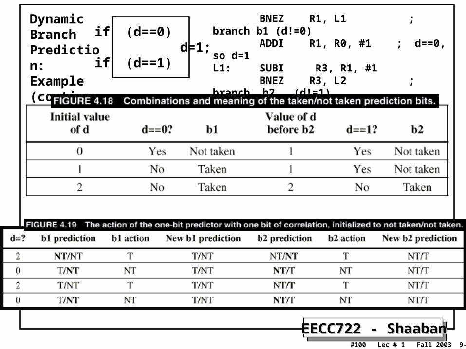
BNEZ R1, L1 ; branch b1 (d!=0)ADDI R1, R0, #1 ; d==0, so d=1
L1: SUBI R3, R1, #1BNEZ R3, L2 ; branch b2 (d!=1)
. . .L2:
Dynamic Branch Prediction: Example
if (d==0) d=1;if (d==1)
EECC722 - ShaabanEECC722 - Shaaban#100 Lec # 1 Fall 2003 9-8-2003
BNEZ R1, L1 ; branch b1 (d!=0)ADDI R1, R0, #1 ; d==0, so d=1
L1: SUBI R3, R1, #1BNEZ R3, L2 ; branch b2 (d!=1)
. . .L2:
if (d==0) d=1;if (d==1)
Dynamic Branch Prediction:Example(continued)

EECC722 - ShaabanEECC722 - Shaaban#101 Lec # 1 Fall 2003 9-8-2003
Organization of A Correlating Two-level GAp (2,2) Branch Predictor
First Level(2 bit shift register)
Second Level
m = # of branches tracked in first level = 2Thus 2m = 22 = 4 tables in second level
N = # of low bits of branch address used = 4Thus each table in 2nd level has 2N = 24 = 16 entries
n = # number of bits of 2nd level table entry = 2
Number of bits for 2nd level = 2m x n x 2N = 4 x 2 x 16 = 128 bits
High bit determines branch prediction0 = Not Taken1 = Taken
Low 4 bits of address
Selects correct table
Selects correct entry in table
GAp
Global(1st level) Adaptive
per address(2nd level)

EECC722 - ShaabanEECC722 - Shaaban#102 Lec # 1 Fall 2003 9-8-2003
Prediction Accuracy Prediction Accuracy of Two-Bit Dynamic of Two-Bit Dynamic Predictors Under Predictors Under SPEC89SPEC89
BasicBasic BasicBasic Correlating Correlating Two-levelTwo-level
GAp

EECC722 - ShaabanEECC722 - Shaaban#103 Lec # 1 Fall 2003 9-8-2003
Multiple Instruction Issue: CPI < 1Multiple Instruction Issue: CPI < 1 • To improve a pipeline’s CPI to be better [less] than one, and to utilize ILP
better, a number of independent instructions have to be issued in the same pipeline cycle.
• Multiple instruction issue processors are of two types:– Superscalar: A number of instructions (2-8) is issued in the same
cycle, scheduled statically by the compiler or dynamically (Tomasulo).
• PowerPC, Sun UltraSparc, Alpha, HP 8000 ...
– VLIW (Very Long Instruction Word): A fixed number of instructions (3-6) are formatted as one long
instruction word or packet (statically scheduled by the compiler). – Joint HP/Intel agreement (Itanium, Q4 2000).– Intel Architecture-64 (IA-64) 64-bit address:
• Explicitly Parallel Instruction Computer (EPIC): Itanium.
• Limitations of the approaches:– Available ILP in the program (both).– Specific hardware implementation difficulties (superscalar).– VLIW optimal compiler design issues.

EECC722 - ShaabanEECC722 - Shaaban#104 Lec # 1 Fall 2003 9-8-2003
Multiple Instruction Issue:Multiple Instruction Issue:
SuperscalarSuperscalar Vs. Vs. VLIWVLIW
• Smaller code size.
• Binary compatibility across generations of hardware.
• Simplified Hardware for decoding, issuing instructions.
• No Interlock Hardware (compiler checks?)
• More registers, but simplified hardware for register ports.

EECC722 - ShaabanEECC722 - Shaaban#105 Lec # 1 Fall 2003 9-8-2003
• Two instructions can be issued per cycle (two-issue superscalar).
• One of the instructions is integer (including load/store, branch). The other instruction is a floating-point operation.
– This restriction reduces the complexity of hazard checking.
• Hardware must fetch and decode two instructions per cycle.
• Then it determines whether zero (a stall), one or two instructions can be issued per cycle.
Simple Statically Scheduled Superscalar PipelineSimple Statically Scheduled Superscalar Pipeline
MEM
EX
EX
EX
ID
ID
IF
IF
EX
EX
ID
ID
IF
IF
WB
WB
EX
MEM
EX
EX
EX
WB
WB
EX
MEM
EX
WB
WB
EX
ID
ID
IF
IF
WB
EX
MEM
EX
EX
EX
ID
ID
IF
IF
Integer Instruction
Integer Instruction
Integer Instruction
Integer Instruction
FP Instruction
FP Instruction
FP Instruction
FP Instruction
1 2 3 4 5 6 7 8Instruction Type
Two-issue statically scheduled pipeline in operationTwo-issue statically scheduled pipeline in operationFP instructions assumed to be addsFP instructions assumed to be adds

EECC722 - ShaabanEECC722 - Shaaban#106 Lec # 1 Fall 2003 9-8-2003
Intel/HP VLIW “Explicitly Parallel Intel/HP VLIW “Explicitly Parallel Instruction Computing (EPIC)”Instruction Computing (EPIC)”
• Three instructions in 128 bit “Groups”; instruction template fields determines if instructions are dependent or independent– Smaller code size than old VLIW, larger than x86/RISC– Groups can be linked to show dependencies of more than three
instructions.
• 128 integer registers + 128 floating point registers– No separate register files per functional unit as in old VLIW.
• Hardware checks dependencies (interlocks binary compatibility over time)
• Predicated execution: An implementation of conditional instructions used to reduce the number of conditional branches used in the generated code larger basic block size
• IA-64 : Name given to instruction set architecture (ISA).• Itanium : Name of the first implementation (2001).

EECC722 - ShaabanEECC722 - Shaaban#107 Lec # 1 Fall 2003 9-8-2003
Intel/HP EPIC VLIW ApproachIntel/HP EPIC VLIW Approachoriginal sourceoriginal source
codecode
ExposeExposeInstructionInstructionParallelismParallelism
OptimizeOptimizeExploitExploit
Parallelism:Parallelism:GenerateGenerate
VLIWsVLIWs
compilercompiler
Instruction DependencyInstruction DependencyAnalysisAnalysis
Instruction 2Instruction 2 Instruction 1Instruction 1 Instruction 0Instruction 0 TemplateTemplate
128-bit bundle128-bit bundle
00127127

EECC722 - ShaabanEECC722 - Shaaban#108 Lec # 1 Fall 2003 9-8-2003
Unrolled Loop Example for Scalar PipelineUnrolled Loop Example for Scalar Pipeline
1 Loop: L.D F0,0(R1)2 L.D F6,-8(R1)3 L.D F10,-16(R1)4 L.D F14,-24(R1)5 ADD.D F4,F0,F26 ADD.D F8,F6,F27 ADD.D F12,F10,F28 ADD.D F16,F14,F29 S.D F4,0(R1)10 S.D F8,-8(R1)11 DADDUI R1,R1,#-3212 S.D F12,-16(R1)13 BNE R1,R2,LOOP14 S.D F16,8(R1) ; 8-32 = -24
14 clock cycles, or 3.5 per iteration
L.D to ADD.D: 1 CycleADD.D to S.D: 2 Cycles

EECC722 - ShaabanEECC722 - Shaaban#109 Lec # 1 Fall 2003 9-8-2003
Loop Unrolling in Superscalar Pipeline: Loop Unrolling in Superscalar Pipeline: (1 Integer, 1 FP/Cycle)(1 Integer, 1 FP/Cycle)
Integer instruction FP instruction Clock cycle
Loop: L.D F0,0(R1) 1
L.D F6,-8(R1) 2
L.D F10,-16(R1) ADD.D F4,F0,F2 3
L.D F14,-24(R1) ADD.D F8,F6,F2 4
L.D F18,-32(R1) ADD.D F12,F10,F2 5
S.D F4,0(R1) ADD.D F16,F14,F2 6
S.D F8,-8(R1) ADD.D F20,F18,F2 7
S.D F12,-16(R1) 8
DADDUI R1,R1,#-40 9
S.D F16,-24(R1) 10
BNE R1,R2,LOOP 11
SD -32(R1),F20 12
• Unrolled 5 times to avoid delays (+1 due to SS)• 12 clocks, or 2.4 clocks per iteration (1.5X)• 7 issue slots wasted

EECC722 - ShaabanEECC722 - Shaaban#110 Lec # 1 Fall 2003 9-8-2003
Loop Unrolling in VLIW PipelineLoop Unrolling in VLIW Pipeline(2 Memory, 2 FP, 1 Integer / Cycle)(2 Memory, 2 FP, 1 Integer / Cycle)
Memory Memory FP FP Int. op/ Clockreference 1 reference 2 operation 1 op. 2 branchL.D F0,0(R1) L.D F6,-8(R1) 1
L.D F10,-16(R1) L.D F14,-24(R1) 2
L.D F18,-32(R1) L.D F22,-40(R1) ADD.D F4,F0,F2 ADD.D F8,F6,F2 3
L.D F26,-48(R1) ADD.D F12,F10,F2 ADD.D F16,F14,F2 4
ADD.D F20,F18,F2 ADD.D F24,F22,F2 5
S.D F4,0(R1) S.D F8, -8(R1) ADD.D F28,F26,F2 6
S.D F12, -16(R1) S.D F16,-24(R1) DADDUI R1,R1,#-56 7
S.D F20, 24(R1) S.D F24,16(R1) 8
S.D F28, 8(R1) BNE R1,R2,LOOP 9
Unrolled 7 times to avoid delays 7 results in 9 clocks, or 1.3 clocks per iteration (1.8X) Average: 2.5 ops per clock, 50% efficiency Note: Needs more registers in VLIW (15 vs. 6 in Superscalar)

EECC722 - ShaabanEECC722 - Shaaban#111 Lec # 1 Fall 2003 9-8-2003
Superscalar Dynamic SchedulingSuperscalar Dynamic Scheduling• How to issue two instructions and keep in-order instruction
issue for Tomasulo?– Assume: 1 integer + 1 floating-point operations. – 1 Tomasulo control for integer, 1 for floating point.
• Issue at 2X Clock Rate, so that issue remains in order.
• Only FP loads might cause a dependency between integer and FP issue:– Replace load reservation station with a load queue;
operands must be read in the order they are fetched.– Load checks addresses in Store Queue to avoid RAW
violation– Store checks addresses in Load Queue to avoid WAR,
WAW.• Called “Decoupled Architecture”

EECC722 - ShaabanEECC722 - Shaaban#112 Lec # 1 Fall 2003 9-8-2003
Multiple Instruction Issue ChallengesMultiple Instruction Issue Challenges• While a two-issue single Integer/FP split is simple in hardware, we get
a CPI of 0.5 only for programs with:
– Exactly 50% FP operations– No hazards of any type.
• If more instructions issue at the same time, greater difficulty of decode and issue operations arise:– Even for a 2-issue superscalar machine, we have to examine 2
opcodes, 6 register specifiers, and decide if 1 or 2 instructions can issue.
• VLIW: tradeoff instruction space for simple decoding
– The long instruction word has room for many operations.
– By definition, all the operations the compiler puts in the long instruction word are independent => execute in parallel
– E.g. 2 integer operations, 2 FP ops, 2 Memory refs, 1 branch• 16 to 24 bits per field => 7*16 or 112 bits to 7*24 or 168 bits wide
– Need compiling technique that schedules across several branches.

EECC722 - ShaabanEECC722 - Shaaban#113 Lec # 1 Fall 2003 9-8-2003
Limits to Multiple Instruction Issue Limits to Multiple Instruction Issue MachinesMachines• Inherent limitations of ILP:
– If 1 branch exist for every 5 instruction : How to keep a 5-way VLIW busy?– Latencies of unit adds complexity to the many operations that must be scheduled
every cycle.– For maximum performance multiple instruction issue requires about: Pipeline Depth x No. Functional Units
independent instructions per cycle.
• Hardware implementation complexities:– Duplicate FUs for parallel execution are needed.– More instruction bandwidth is essential.– Increased number of ports to Register File (datapath bandwidth):
• VLIW example needs 7 read and 3 write for Int. Reg. & 5 read and 3 write for FP reg
– Increased ports to memory (to improve memory bandwidth).
– Superscalar decoding complexity may impact pipeline clock rate.

EECC722 - ShaabanEECC722 - Shaaban#114 Lec # 1 Fall 2003 9-8-2003
• Empty or wasted issue slots can be defined as either vertical waste or horizontal waste:
– Vertical waste is introduced when the processor issues no instructions in a cycle.
– Horizontal waste occurs when not all issue slots can be filled in a cycle.
Superscalar Architectures:Superscalar Architectures:Issue Slot Waste Classification

EECC722 - ShaabanEECC722 - Shaaban#115 Lec # 1 Fall 2003 9-8-2003
Hardware Support for Extracting More ParallelismHardware Support for Extracting More Parallelism• Compiler ILP techniques (loop-unrolling, software Pipelining etc.) are
not effective to uncover maximum ILP when branch behavior is not well known at compile time.
• Hardware ILP techniques:
– Conditional or Predicted Instructions: An extension to the instruction set with instructions that turn into no-ops if a condition is not valid at run time.
– Speculation: An instruction is executed before the processor knows that the instruction should execute to avoid control dependence stalls:
• Static Speculation by the compiler with hardware support:– The compiler labels an instruction as speculative and the hardware helps
by ignoring the outcome of incorrectly speculated instructions.
– Conditional instructions provide limited speculation.
• Dynamic Hardware-based Speculation:– Uses dynamic branch-prediction to guide the speculation process.
– Dynamic scheduling and execution continued passed a conditional branch in the predicted branch direction.

EECC722 - ShaabanEECC722 - Shaaban#116 Lec # 1 Fall 2003 9-8-2003
Conditional or Predicted InstructionsConditional or Predicted Instructions• Avoid branch prediction by turning branches into
conditionally-executed instructions:
if (x) then (A = B op C) else NOP– If false, then neither store result nor cause exception:
instruction is annulled (turned into NOP) .– Expanded ISA of Alpha, MIPS, PowerPC, SPARC have
conditional move.– HP PA-RISC can annul any following instruction.– IA-64: 64 1-bit condition fields selected so conditional execution of any instruction
(Predication).
• Drawbacks of conditional instructions– Still takes a clock cycle even if “annulled”.
– Must stall if condition is evaluated late.– Complex conditions reduce effectiveness;
condition becomes known late in pipeline.
x
A = B op C

EECC722 - ShaabanEECC722 - Shaaban#117 Lec # 1 Fall 2003 9-8-2003
Dynamic Hardware-Based SpeculationDynamic Hardware-Based Speculation• Combines:Combines:
– Dynamic hardware-based branch prediction– Dynamic Scheduling: of multiple instructions to issue and
execute out of order.
• Continue to dynamically issue, and execute instructions passed a conditional branch in the dynamically predicted branch direction, before control dependencies are resolved.– This overcomes the ILP limitations of the basic block size.– Creates dynamically speculated instructions at run-time with no
compiler support at all.– If a branch turns out as mispredicted all such dynamically
speculated instructions must be prevented from changing the state of the machine (registers, memory).
• Addition of commit (retire or re-ordering) stage and forcing instructions to commit in their order in the code (i.e to write results to registers or memory).
• Precise exceptions are possible since instructions must commit in order.

EECC722 - ShaabanEECC722 - Shaaban#118 Lec # 1 Fall 2003 9-8-2003
Hardware-Based Hardware-Based SpeculationSpeculation
Speculative Execution +Speculative Execution + Tomasulo’s AlgorithmTomasulo’s Algorithm

EECC722 - ShaabanEECC722 - Shaaban#119 Lec # 1 Fall 2003 9-8-2003
Four Steps of Speculative Tomasulo AlgorithmFour Steps of Speculative Tomasulo Algorithm1. Issue — Get an instruction from FP Op Queue
If a reservation station and a reorder buffer slot are free, issue instruction & send operands & reorder buffer number for destination (this stage is sometimes called “dispatch”)
2. Execution — Operate on operands (EX) When both operands are ready then execute; if not ready, watch CDB for
result; when both operands are in reservation station, execute; checks RAW (sometimes called “issue”)
3. Write result — Finish execution (WB) Write on Common Data Bus to all awaiting FUs & reorder buffer; mark
reservation station available.
4. Commit — Update registers, memory with reorder buffer result– When an instruction is at head of reorder buffer & the result is present,
update register with result (or store to memory) and remove instruction from reorder buffer.
– A mispredicted branch at the head of the reorder buffer flushes the reorder buffer (sometimes called “graduation”)
Instructions issue in order, execute (EX), write result (WB) out of order, but must commit in order.

EECC722 - ShaabanEECC722 - Shaaban#120 Lec # 1 Fall 2003 9-8-2003
Advantages of HW (Tomasulo) vs. SW Advantages of HW (Tomasulo) vs. SW (VLIW) Speculation(VLIW) Speculation
• HW determines address conflicts.• HW provides better branch prediction.• HW maintains precise exception model.• HW does not execute bookkeeping instructions.• Works across multiple implementations• SW speculation is much easier for HW design.

EECC722 - ShaabanEECC722 - Shaaban#121 Lec # 1 Fall 2003 9-8-2003
Memory Hierarchy: The motivationMemory Hierarchy: The motivation• The gap between CPU performance and main memory has been
widening with higher performance CPUs creating performance bottlenecks for memory access instructions.
• The memory hierarchy is organized into several levels of memory with the smaller, more expensive, and faster memory levels closer to the CPU: registers, then primary Cache Level (L1), then additional secondary cache levels (L2, L3…), then main memory, then mass storage (virtual memory).
• Each level of the hierarchy is a subset of the level below: data found in a level is also found in the level below but at lower speed.
• Each level maps addresses from a larger physical memory to a smaller level of physical memory.
• This concept is greatly aided by the principal of locality both temporal and spatial which indicates that programs tend to reuse data and instructions that they have used recently or those stored in their vicinity leading to working set of a program.

EECC722 - ShaabanEECC722 - Shaaban#122 Lec # 1 Fall 2003 9-8-2003
Memory Hierarchy: MotivationMemory Hierarchy: MotivationProcessor-Memory (DRAM) Performance GapProcessor-Memory (DRAM) Performance Gap
µProc60%/yr.
DRAM7%/yr.
1
10
100
1000198
0198
1 198
3198
4198
5 198
6198
7198
8198
9199
0199
1 199
2199
3199
4199
5199
6199
7199
8 199
9200
0
DRAM
CPU
198
2
Processor-MemoryPerformance Gap:(grows 50% / year)
Per
form
ance

EECC722 - ShaabanEECC722 - Shaaban#123 Lec # 1 Fall 2003 9-8-2003
Processor-DRAM Performance Gap Impact: Processor-DRAM Performance Gap Impact:
Example Example• To illustrate the performance impact, assume a single-issue pipelined CPU
with CPI = 1 using non-ideal memory. • Ignoring other factors, the minimum cost of a full memory access in terms of
number of wasted CPU cycles:
CPU CPU Memory Minimum CPU cycles or Year speed cycle Access instructions wasted MHZ ns ns
1986: 8 125 190 190/125 - 1 = 0.51989: 33 30 165 165/30 -1 = 4.51992: 60 16.6 120 120/16.6 -1 = 6.21996: 200 5 110 110/5 -1 = 211998: 300 3.33 100 100/3.33 -1 = 292000: 1000 1 90 90/1 - 1 = 892002: 2000 .5 80 80/.5 - 1 = 159

EECC722 - ShaabanEECC722 - Shaaban#124 Lec # 1 Fall 2003 9-8-2003
Cache Design & Operation IssuesCache Design & Operation Issues• Q1: Where can a block be placed cache?
(Block placement strategy & Cache organization)– Fully Associative, Set Associative, Direct Mapped.
• Q2: How is a block found if it is in cache? (Block identification)– Tag/Block.
• Q3: Which block should be replaced on a miss? (Block replacement)– Random, LRU.
• Q4: What happens on a write? (Cache write policy)– Write through, write back.

EECC722 - ShaabanEECC722 - Shaaban#125 Lec # 1 Fall 2003 9-8-2003
Cache Organization & Placement StrategiesCache Organization & Placement StrategiesPlacement strategies or mapping of a main memory data block onto
cache block frame addresses divide cache into three organizations:
1 Direct mapped cache: A block can be placed in one location only, given by:
(Block address) MOD (Number of blocks in cache)
2 Fully associative cache: A block can be placed anywhere in cache.
3 Set associative cache: A block can be placed in a restricted set of places, or cache block frames. A set is a group of block frames in the cache. A block is first mapped onto the set and then it can be placed anywhere within the set. The set in this case is chosen by:
(Block address) MOD (Number of sets in cache)
If there are n blocks in a set the cache placement is called n-way set-associative.

EECC722 - ShaabanEECC722 - Shaaban#126 Lec # 1 Fall 2003 9-8-2003
Locating A Data Block in CacheLocating A Data Block in Cache• Each block frame in cache has an address tag.
• The tags of every cache block that might contain the required data are checked in parallel.
• A valid bit is added to the tag to indicate whether this entry contains a valid address.
• The address from the CPU to cache is divided into:
– A block address, further divided into:
• An index field to choose a block set in cache.
(no index field when fully associative).
• A tag field to search and match addresses in the selected set.
– A block offset to select the data from the block.
Block Address BlockOffsetTag Index

EECC722 - ShaabanEECC722 - Shaaban#127 Lec # 1 Fall 2003 9-8-2003
Address Field SizesAddress Field Sizes
Block Address BlockOffsetTag Index
Block offset size = log2(block size)
Index size = log2(Total number of blocks/associativity)
Tag size = address size - index size - offset sizeTag size = address size - index size - offset size
Physical Address Generated by CPU
Mapping function:
Cache set or block frame number = Index = = (Block Address) MOD (Number of Sets)
Number of Sets

EECC722 - ShaabanEECC722 - Shaaban#128 Lec # 1 Fall 2003 9-8-2003
4KB Direct Mapped 4KB Direct Mapped Cache ExampleCache Example
A d d re s s ( s h o w in g b it p o s i t io n s )
2 0 1 0
B y te
o ffs e t
V a l id T a g D a taIn d e x
0
1
2
1 0 2 1
1 0 2 2
1 0 2 3
T a g
In d e x
H i t D a ta
2 0 3 2
3 1 3 0 1 3 1 2 1 1 2 1 0
1K = 1024 BlocksEach block = one word
Can cache up to232 bytes = 4 GBof memory
Mapping function:
Cache Block frame number =(Block address) MOD (1024)
Index fieldTag field
Block offset = 2 bits
Block Address = 30 bits
Tag = 20 bits Index = 10 bits

EECC722 - ShaabanEECC722 - Shaaban#129 Lec # 1 Fall 2003 9-8-2003
4K Four-Way Set Associative Cache:4K Four-Way Set Associative Cache:MIPS Implementation ExampleMIPS Implementation Example
Ad dress
2 2 8
V TagIndex
0
1
2
253
254
255
D ata V Tag D ata V Tag D ata V Tag D ata
3 22 2
4 - to - 1 m ultip lexo r
H it D a ta
123891011123 031 0
IndexField
TagField
1024 block framesEach block = one word4-way set associative256 sets
Can cache up to232 bytes = 4 GBof memory
Block Address = 30 bits
Tag = 22 bits Index = 8 bits Block offset = 2 bits
Mapping Function: Cache Set Number = (Block address) MOD (256)

EECC722 - ShaabanEECC722 - Shaaban#130 Lec # 1 Fall 2003 9-8-2003
Cache Performance:Average Memory Access Time (AMAT), Memory Stall cycles
• The Average Memory Access Time (AMAT): The number of cycles required to complete an average memory access request by the CPU.
• Memory stall cycles per memory access: The number of stall cycles added to CPU execution cycles for one memory access.
• For ideal memory: AMAT = 1 cycle, this results in zero memory stall cycles.
• Memory stall cycles per average memory access = (AMAT -1)
• Memory stall cycles per average instruction =
Memory stall cycles per average memory access
x Number of memory accesses per instruction
= (AMAT -1 ) x ( 1 + fraction of loads/stores)
Instruction Fetch

EECC722 - ShaabanEECC722 - Shaaban#131 Lec # 1 Fall 2003 9-8-2003
Cache PerformanceCache PerformanceFor a CPU with a single level (L1) of cache and no stalls for
cache hits:
CPU time = (CPU execution clock cycles +
Memory stall clock cycles) x clock cycle time
Memory stall clock cycles = (Reads x Read miss rate x Read miss penalty) + (Writes x Write miss rate x Write miss penalty)
If write and read miss penalties are the same:
Memory stall clock cycles = Memory accesses x Miss rate x Miss penalty
With ideal memory

EECC722 - ShaabanEECC722 - Shaaban#132 Lec # 1 Fall 2003 9-8-2003
Miss Rates for Caches with Different Size, Miss Rates for Caches with Different Size, Associativity & Replacement AlgorithmAssociativity & Replacement Algorithm
Sample DataSample Data
Associativity: 2-way 4-way 8-way
Size LRU Random LRU Random LRURandom
16 KB 5.18% 5.69% 4.67% 5.29% 4.39% 4.96%
64 KB 1.88% 2.01% 1.54% 1.66% 1.39% 1.53%
256 KB 1.15% 1.17% 1.13% 1.13% 1.12% 1.12%

EECC722 - ShaabanEECC722 - Shaaban#133 Lec # 1 Fall 2003 9-8-2003
Typical Cache Performance DataTypical Cache Performance Data Using SPEC92Using SPEC92

EECC722 - ShaabanEECC722 - Shaaban#134 Lec # 1 Fall 2003 9-8-2003
Cache Read/Write OperationsCache Read/Write Operations• Statistical data suggest that reads (including instruction
fetches) dominate processor cache accesses (writes account for 25% of data cache traffic).
• In cache reads, a block is read at the same time while the tag is being compared with the block address. If the read is a hit the data is passed to the CPU, if a miss it ignores it.
• In cache writes, modifying the block cannot begin until the tag is checked to see if the address is a hit.
• Thus for cache writes, tag checking cannot take place in parallel, and only the specific data (between 1 and 8 bytes) requested by the CPU can be modified.
• Cache is classified according to the write and memory update strategy in place: write through, or write back.

EECC722 - ShaabanEECC722 - Shaaban#135 Lec # 1 Fall 2003 9-8-2003
Cache Write StrategiesCache Write Strategies1 Write Though: Data is written to both the cache block and to a
block of main memory.
– The lower level always has the most updated data; an important feature for I/O and multiprocessing.
– Easier to implement than write back.
– A write buffer is often used to reduce CPU write stall while data is written to memory.
2 Write back: Data is written or updated only to the cache block. The modified cache block is written to main memory when it’s being replaced from cache.
– Writes occur at the speed of cache– A status bit called a dirty bit, is used to indicate whether the block
was modified while in cache; if not the block is not written to main memory.
– Uses less memory bandwidth than write through.

EECC722 - ShaabanEECC722 - Shaaban#136 Lec # 1 Fall 2003 9-8-2003
Cache Write Miss PolicyCache Write Miss Policy• Since data is usually not needed immediately on a write miss
two options exist on a cache write miss:
Write Allocate:
The cache block is loaded on a write miss followed by write hit actions.
No-Write Allocate:
The block is modified in the lower level (lower cache level, or main
memory) and not loaded into cache.
While any of the above two write miss policies can be used with either write back or write through:
• Write back caches use write allocate to capture subsequent writes to the block in cache.
• Write through caches usually use no-write allocate since subsequent writes still have to go to memory.

EECC722 - ShaabanEECC722 - Shaaban#137 Lec # 1 Fall 2003 9-8-2003
Memory Access Tree, Unified L1
Write Through, No Write Allocate, No Write Buffer
CPU Memory Access
L1
Read Write
L1 Write Miss:Access Time : M + 1Stalls per access: % write x (1 - H1 ) x M
L1 Write Hit:Access Time: M +1 Stalls Per access:% write x (H1 ) x M
L1 Read Hit:Access Time = 1Stalls = 0
L1 Read Miss:Access Time = M + 1Stalls Per access
% reads x (1 - H1 ) x M
Stall Cycles Per Memory Access = % reads x (1 - H1 ) x M + % write x M
AMAT = 1 + % reads x (1 - H1 ) x M + % write x M

EECC722 - ShaabanEECC722 - Shaaban#138 Lec # 1 Fall 2003 9-8-2003
Write Write Through Cache Performance Example Cache Performance Example• A CPU with CPIexecution = 1.1 uses a unified L1 Write Through, No Write
Allocate and no write buffer.
• Instruction mix: 50% arith/logic, 15% load, 15% store, 20% control
• Assume a cache miss rate of 1.5% and a miss penalty of 50 cycles.
CPI = CPIexecution + mem stalls per instruction
Mem Stalls per instruction =
Mem accesses per instruction x Stalls per access
Mem accesses per instruction = 1 + .3 = 1.3 Stalls per access = % reads x miss rate x Miss penalty + % write x Miss penalty
% reads = 1.15/1.3 = 88.5% % writes = .15/1.3 = 11.5%
Stalls per access = 50 x (88.5% x 1.5% + 11.5%) = 6.4 cycles
Mem Stalls per instruction = 1.3 x 6.4 = 8.33 cycles
AMAT = 1 + 8.33 = 9.33 cycles
CPI = 1.1 + 8.33 = 9.43
The ideal memory CPU with no misses is 9.43/1.1 = 8.57 times faster

EECC722 - ShaabanEECC722 - Shaaban#139 Lec # 1 Fall 2003 9-8-2003
Memory Access Tree Unified L1
Write Back, With Write Allocate CPU Memory Access
L1
Read Write
L1 Write Miss L1 Write Hit:% write x H1Access Time = 1Stalls = 0
L1 Hit:% read x H1Access Time = 1Stalls = 0
L1 Read Miss
Stall Cycles Per Memory Access = (1-H1) x ( M x % clean + 2M x % dirty )
AMAT = 1 + Stall Cycles Per Memory Access
CleanAccess Time = M +1Stall cycles = M x (1-H1 ) x % reads x % clean
DirtyAccess Time = 2M +1Stall cycles = 2M x (1-H1) x %read x % dirty
CleanAccess Time = M +1Stall cycles = M x (1 -H1) x % write x % clean
DirtyAccess Time = 2M +1Stall cycles = 2M x (1-H1) x %read x % dirty

EECC722 - ShaabanEECC722 - Shaaban#140 Lec # 1 Fall 2003 9-8-2003
Write Back Cache Performance ExampleWrite Back Cache Performance Example• A CPU with CPIexecution = 1.1 uses a unified L1 with with write back , with
write allocate, and the probability a cache block is dirty = 10% • Instruction mix: 50% arith/logic, 15% load, 15% store, 20% control
• Assume a cache miss rate of 1.5% and a miss penalty of 50 cycles.
CPI = CPIexecution + mem stalls per instruction
Mem Stalls per instruction =
Mem accesses per instruction x Stalls per access
Mem accesses per instruction = 1 + .3 = 1.3
Stalls per access = (1-H1) x ( M x % clean + 2M x % dirty )
Stalls per access = 1.5% x (50 x 90% + 100 x 10%) = .825 cycles
Mem Stalls per instruction = 1.3 x .825 = 1.07 cycles
AMAT = 1 + 1.07 = 2.07 cycles
CPI = 1.1 + 1.07 = 2.17
The ideal CPU with no misses is 2.17/1.1 = 1.97 times faster

EECC722 - ShaabanEECC722 - Shaaban#141 Lec # 1 Fall 2003 9-8-2003
Miss Rates For Multi-Level CachesMiss Rates For Multi-Level Caches• Local Miss Rate: This rate is the number of misses in a
cache level divided by the number of memory accesses to this level. Local Hit Rate = 1 - Local Miss Rate
• Global Miss Rate: The number of misses in a cache level divided by the total number of memory accesses generated by the CPU.
• Since level 1 receives all CPU memory accesses, for level 1:– Local Miss Rate = Global Miss Rate = 1 - H1
• For level 2 since it only receives those accesses missed in 1:
– Local Miss Rate = Miss rateL2= 1- H2
– Global Miss Rate = Miss rateL1 x Miss rateL2
= (1- H1) x (1 - H2)

EECC722 - ShaabanEECC722 - Shaaban#142 Lec # 1 Fall 2003 9-8-2003
2-Level Cache Performance 2-Level Cache Performance Memory Access TreeMemory Access Tree
CPU Stall Cycles Per Memory AccessCPU Stall Cycles Per Memory Access
CPU Memory Access
L1 Miss: % = (1-H1)
L1 Hit:Stalls= H1 x 0 = 0(No Stall)
L2 Miss: Stalls= (1-H1)(1-H2) x M
L2 Hit:(1-H1) x H2 x T2
Stall cycles per memory access = (1-H1) x H2 x T2 + (1-H1)(1-H2) x MAMAT = 1 + (1-H1) x H2 x T2 + (1-H1)(1-H2) x M
L1
L2

EECC722 - ShaabanEECC722 - Shaaban#143 Lec # 1 Fall 2003 9-8-2003
3 Levels of Cache3 Levels of Cache
CPU
L1 Cache
L2 Cache
L3 Cache
Main Memory
Hit Rate= H1, Hit time = 1 cycle
Hit Rate= H2, Hit time = T2 cycles
Hit Rate= H3, Hit time = T3
Memory access penalty, M

EECC722 - ShaabanEECC722 - Shaaban#144 Lec # 1 Fall 2003 9-8-2003
3-Level Cache Performance 3-Level Cache Performance Memory Access TreeMemory Access Tree
CPU Stall Cycles Per Memory AccessCPU Stall Cycles Per Memory Access
CPU Memory Access
L1 Miss: % = (1-H1)
L1 Hit:Stalls= H1 x 0 = 0 ( No Stall)
L2 Miss: % = (1-H1)(1-H2)
L2 Hit:(1-H1) x H2 x T2
Stall cycles per memory access = (1-H1) x H2 x T2 + (1-H1) x (1-H2) x H3 x T3 + (1-H1)(1-H2) (1-H3)x MAMAT = 1 + Stall cycles per memory access
L3 Miss: (1-H1)(1-H2)(1-H3) x M
L3 Hit:(1-H1) x (1-H2) x H3 x T3
L1
L3
L2

EECC722 - ShaabanEECC722 - Shaaban#145 Lec # 1 Fall 2003 9-8-2003
Three-Level Cache ExampleThree-Level Cache Example• CPU with CPIexecution = 1.1 running at clock rate = 500 MHZ• 1.3 memory accesses per instruction.• L1 cache operates at 500 MHZ with a miss rate of 5%• L2 cache operates at 250 MHZ with a local miss rate 40%, (T2 = 2 cycles)• L3 cache operates at 100 MHZ with a local miss rate 50%, (T3 = 5 cycles)• Memory access penalty, M= 100 cycles. Find CPI. With No Cache, CPI = 1.1 + 1.3 x 100 = 131.1
With single L1, CPI = 1.1 + 1.3 x .05 x 100 = 7.6
With L1, L2 CPI = 1.1 + 1.3 x (.05 x .6 x 2 + .05 x .4 x 100) = 3.778
CPI = CPIexecution + Mem Stall cycles per instruction
Mem Stall cycles per instruction = Mem accesses per instruction x Stall cycles per access
Stall cycles per memory access = (1-H1) x H2 x T2 + (1-H1) x (1-H2) x H3 x T3 + (1-H1)(1-H2) (1-H3)x M
= .05 x .6 x 2 + .05 x .4 x .5 x 5 + .05 x .4 x .5 x 100 = .097 + .0075 + .00225 = 1.11
CPI = 1.1 + 1.3 x 1.11 = 2.54 Speedup compared to L1 only = 7.6/2.54 = 3
Speedup compared to L1, L2 = 3.778/2.54 = 1.49

EECC722 - ShaabanEECC722 - Shaaban#146 Lec # 1 Fall 2003 9-8-2003
Cache Optimization SummaryCache Optimization SummaryTechnique MR MP HT Complexity
Larger Block Size + – 0Higher Associativity + – 1Victim Caches + 2Pseudo-Associative Caches + 2HW Prefetching of Instr/Data + 2Compiler Controlled Prefetching + 3Compiler Reduce Misses + 0
Priority to Read Misses + 1Subblock Placement + + 1Early Restart & Critical Word 1st + 2Non-Blocking Caches + 3Second Level Caches + 2
Small & Simple Caches – + 0Avoiding Address Translation + 2Pipelining Writes + 1
Mis
s ra
teH
it t
ime
Mis
sP
enal
ty

EECC722 - ShaabanEECC722 - Shaaban#147 Lec # 1 Fall 2003 9-8-2003
X86 CPU Cache/Memory Performance Example:X86 CPU Cache/Memory Performance Example:AMD Athlon T-Bird Vs. Intel PIII, Vs. P4AMD Athlon T-Bird Vs. Intel PIII, Vs. P4
AMD Athlon T-Bird 1GHZL1: 64K INST, 64K DATA (3 cycle latency), both 2-wayL2: 256K 16-way 64 bit Latency: 7 cycles L1,L2 on-chip
Intel PIII 1 GHZL1: 16K INST, 16K DATA (3 cycle latency) both 4-wayL2: 256K 8-way 256 bit , Latency: 7 cycles
L1,L2 on-chip
Intel P 4, 1.5 GHZL1: 8K INST, 8K DATA (2 cycle latency) both 4-way 96KB Execution Trace CacheL2: 256K 8-way 256 bit , Latency: 7 cycles
L1,L2 on-chip
Source: http://www1.anandtech.com/showdoc.html?i=1360&p=15
Intel P4 utilizes PC800 bandwidth much better than PIII due to P4’s higher 400MHZ system bus speed.