© Copyright ARRI/ACS 2004 All rights reserved

EE 4343/5320 - Control System Design Project Updated: Friday, February 13, 2004

Bode Plots Bode plot methods give a graphical procedure for determining the stability of a control system based on response for frequency dependent inputs. Time domain methods study the behavior of the system for the inputs which are functions of time; Frequency domain methods do the same but for frequency based functions. H(s) (Open loop transfer function) H (jω ) (Function of a complex variable) A complex variable function of frequency ω We know that one can express a complex variable in terms of magnitude and phase angle. BODE PLOT Plots of 1. (Variation of Magnitude of Transfer Function) dB Vs (Frequency) logarithmic

AND

2. (Variation of Corresponding Phase Angle) degrees Vs (Frequency) logarithmic Advantage:

• Logarithmic bode plot has an advantage of being approximated by asymptotic Straight lines.

• Relative Stability of a closed loop system control system can be assessed. • Gain margin can directly be determined.

Limitations:??

1

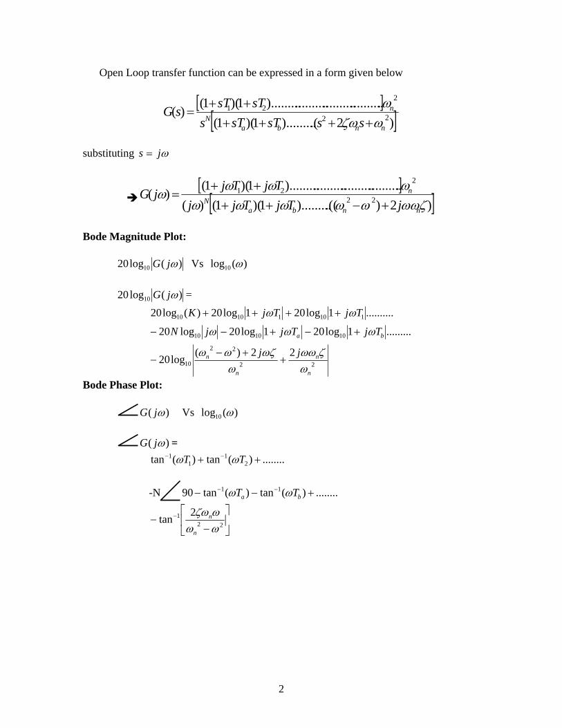
Open Loop transfer function can be expressed in a form given below

[ ][ ])2.().........1)(1(

...............................).........1)(1()( 22

221

nnbaN

n

sssTsTssTsTsG

ωζωω

++++++

=

substituting ωjs =

[ ][ ])2).(().........1)(1()(

...............................).........1)(1()( 22

221

ζωωωωωωωωωωω

nnbaN

n

jTjTjjTjTjjG

+−++++

=

Bode Magnitude Plot:

)(log20 10 ωjG Vs )(log10 ω

)(log20 10 ωjG =

22

22

10

101010

11011010

22)(log20

.........1log201log20log20

..........1log201log20)(log20

n

n

n

n

ba

jj

TjTjjN

TjTjK

ωζωω

ωωζωω

ωωω

ωω

++−

−

+−+−−

++++

Bode Phase Plot:

)( ωjG Vs log )(10 ω

)( ωjG = ........)(tan)(tan 2

11

1 ++ −− TT ωω

-N 90 ........)(tan)(tan 11 +−− −−ba TT ωω

⎥⎦

⎤⎢⎣

⎡

−− −

221 2tan

ωωωζω

n

n

2

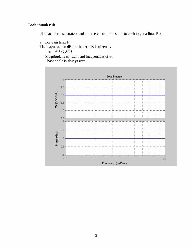
Bode thumb rule:

Plot each term separately and add the contributions due to each to get a final Plot. a. For gain term K: The magnitude in dB for the term K is given by

K dB = 20 )(log10 KMagnitude is constant and independent of ω. Phase angle is always zero.

3

b. For the term Nj )(1ω

Magnitude:

Nj )(1log20 10 ω

− = ωjN 10log20−

Equation of a line falling 20N per decade

Phase: 090)(

1 Nj N −=ω

4

c. Graph for the term )1( Tjω+ Magnitude:

( )221010 1log20)1(log20 TTj ωω +=+

Case 1 1<<Tω ( Low frequency) ( ) dBTj 01log20)1(log20 1010 =≈+ ω

Case 2 1>>Tω ( High frequency) ( )

)1(log20)(log20

)(log20log20)1(log20

1010

10

221010

T

dBTTTj

−=

=

≈+

ω

ωωω

Has a slope of 20 dB/decade. Case 1 and Case graphs intersect at point when

)1(log20)(log20 1010 T−ω =0

T1

=ω

Phase:

⎟⎠⎞

⎜⎝⎛= −

1tan 1 Tωφ

Case 1: Low frequency ( ) 01 00tan =≈ −φ

Case 2 : At T1

=ω

01 45*1tan =⎟⎠⎞

⎜⎝⎛= − TT

φ

Case 3: High Frequency ( ) 01 90tan =∞≈ −φ

Figure : Graph for the term (1+.1sT)

5

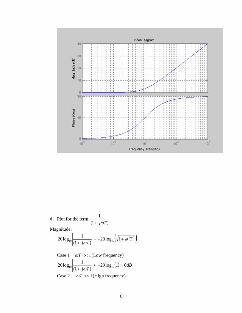
d. Plot for the term )1(

1Tjω+

Magnitude:

( )221010 1log20

)1(1log20 T

Tjω

ω+−=

+

Case 1 1<<Tω (Low frequency)

( ) dBTj

01log20)1(

1log20 1010 =−≈+ ω

Case 2 1>>Tω (High frequency)

6

( )

dBT

dBT

TTj

)1(log20)(log20

)(log20

log20)1(

1log20

1010

10

221010

+−=

−=

−≈+

ω

ω

ωω

Has a slope of -20 dB/decade. Case 1 and Case graphs intersect at point when

)1(log20)(log20 1010 T+− ω =0

T1

=ω

Phase:

⎟⎠⎞

⎜⎝⎛−= −

1tan 1 Tωφ

Case 1: Low frequency ( ) 01 00tan =−≈ −φ

Case 2 : At T1

=ω

01 45*1tan −=⎟⎠⎞

⎜⎝⎛−= − TT

φ

Case 3: High Frequency ( ) 01 90tan −=∞−≈ −φ

Figure : Graph for the term )1.1(

1s+

7

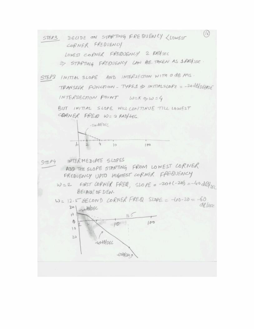
INITIAL SLOPE OF BODE PLOT Corner frequencies due to first order terms

etcTjTj

TjTjba

...........)1(

1,)1(

1.).........1)(1( 21 ωωωω

++++

are given by

etcTTTT ba

...........1,1.........,.........1,1

21=ω

For frequencies lower than the lowest corner frequency the contribution towards the gain(Magnitude in dB) of the transfer function is nil Sinusoidal transfer function for frequencies lower than the lowest corner frequency can be expressed as

NjKjG

)()(

ωω ≅

Magnitude )(log20)(log20)(log20 101010 ωω NKjG −=

For Type N transfer function magnitude has initial slope of -20NdB/decade. Intersection with 0 dB axis

)(log20)(log20 1010 ωNK − =0

8

( ) NK1

=ω

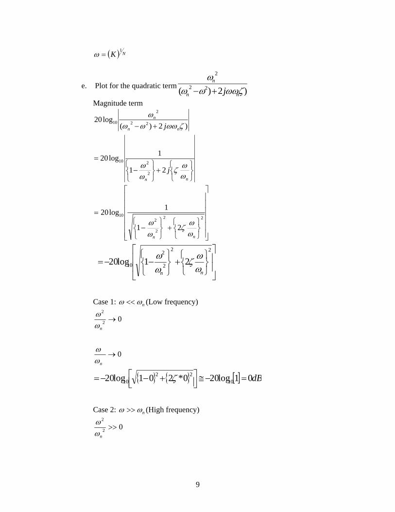
e. Plot for the quadratic term )2)( 22

2

ζωωωωω

nn

n

j+−

Magnitude term

⎭⎬⎫

⎩⎨⎧

+⎭⎬⎫

⎩⎨⎧−

=

+−

nn

nn

n

j

j

ωωζ

ωω

ζωωωωω

21

1log20

)2)(log20

2

210

22

2

10

⎥⎥⎥⎥⎥⎥

⎦

⎤

⎢⎢⎢⎢⎢⎢

⎣

⎡

⎭⎬⎫

⎩⎨⎧

+⎭⎬⎫

⎩⎨⎧−

=22

2

210

21

1log20

nn ωωζ

ωω

⎥⎥

⎦

⎤

⎢⎢

⎣

⎡

⎭⎬⎫

⎩⎨⎧

+⎭⎬⎫

⎩⎨⎧−−=

22

2

2

10 21log20nn ωωζ

ωω

Case 1: nωω << (Low frequency)

02

2

→nω

ω

0→nω

ω

{ } { } [ ] dB01log200*201log20 1022

10 =−≅⎥⎦⎤

⎢⎣⎡ +−−= ζ

Case 2: nωω >> (High frequency)

02

2

>>nω

ω

9

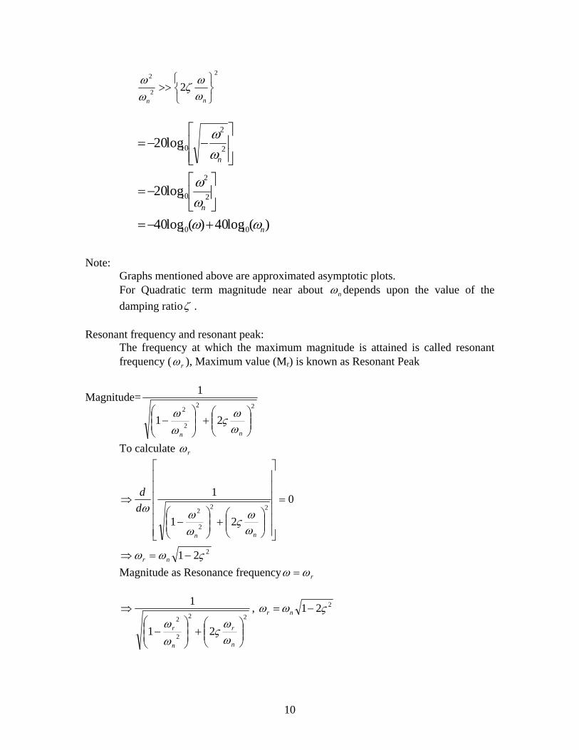
2

2

2

2⎭⎬⎫

⎩⎨⎧

>>nn ωωζ

ωω

)(log40)(log40

log20

log20

1010

2

2

10

2

2

10

n

n

n

ωωωω

ωω

+−=

⎥⎦

⎤⎢⎣

⎡−=

⎥⎥⎦

⎤

⎢⎢⎣

⎡−−=

Note: Graphs mentioned above are approximated asymptotic plots. For Quadratic term magnitude near about nω depends upon the value of the damping ratioζ .

Resonant frequency and resonant peak: The frequency at which the maximum magnitude is attained is called resonant frequency ( rω ), Maximum value (Mr) is known as Resonant Peak

Magnitude=22

2

2

21

1

⎟⎟⎠

⎞⎜⎜⎝

⎛+⎟

⎟⎠

⎞⎜⎜⎝

⎛−

nn ωως

ωω

To calculate rω

2

22

2

2

21

0

21

1

ςωω

ωως

ωωω

−=⇒

=

⎥⎥⎥⎥⎥⎥

⎦

⎤

⎢⎢⎢⎢⎢⎢

⎣

⎡

⎟⎟⎠

⎞⎜⎜⎝

⎛+⎟⎟

⎠

⎞⎜⎜⎝

⎛−

⇒

nr

nn

dd

Magnitude as Resonance frequency rωω =

22

2

2

21

1

⎟⎟⎠

⎞⎜⎜⎝

⎛+⎟

⎟⎠

⎞⎜⎜⎝

⎛−

⇒

n

r

n

r

ωω

ςωω

, 221 ςωω −= nr

10

( )

( )⎥⎥⎦

⎤

⎢⎢⎣

⎡

−=⇒

−=⇒

210

2

121log20)(

121

ςς

ςς

dBM

M

r

r

Phase Angle:

[ ]⎥⎥⎥⎥

⎦

⎤

⎢⎢⎢⎢

⎣

⎡

−=

+−∠ −

2

21

22

2

1

2tan

2)(

n

n

nn

n

jωωωως

ωωςωωω

At Corner frequency

221 ςωω

ωω

−=

=

nr

r

⎥⎥⎦

⎤

⎢⎢⎣

⎡

−−−=∠ −

2

1

1sin90

ς

ς

11

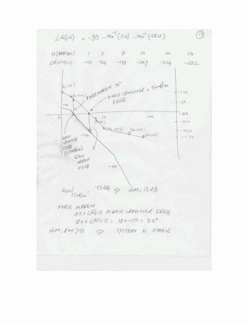
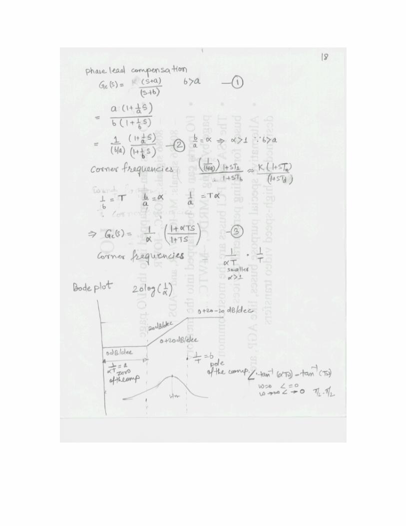
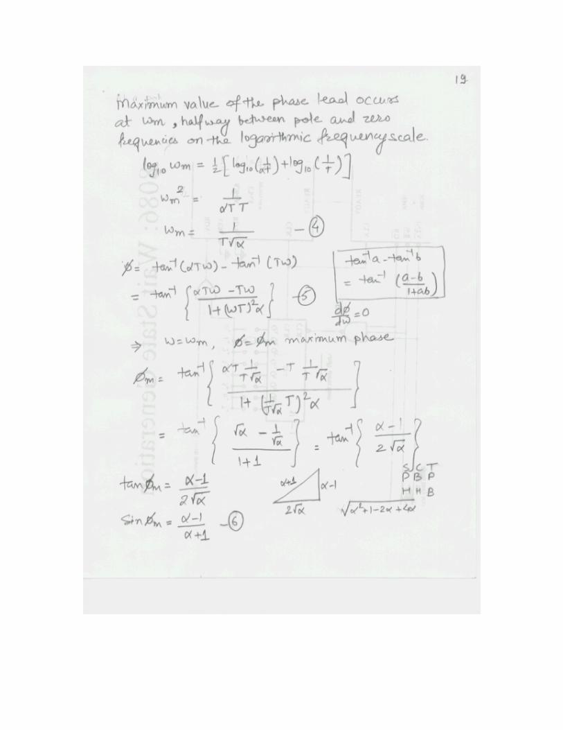
% Example : A lead compensator for a second order system A unity % feedback control system has a loop transfer function 4/(s(s+2)). It is % desired to design a compensator for the system so that satic velocity % error constant is 20, phase margin is 50 and gain margin is atleast 10 % db clear all close all clc % First step in design is to adjust gain K to meet the steady state % performance specifications, we have already obtained k=10. % % MARGIN Gain and phase margins and crossover frequencies. % % [Gm,Pm,Wcg,Wcp] = MARGIN(SYS) computes the gain margin Gm, the % phase margin Pm, and the associated frequencies Wcg and Wcp, % for the SISO open-loop model SYS (continuous or discrete). % The gain margin Gm is defined as 1/G where G is the gain at % the -180 phase crossing. The phase margin Pm is in degrees. % The gain margin in dB is derived by % Gm_dB = 20*log10(Gm) % The loop gain at Wcg can increase or decrease by this many dBs % before losing stability, and Gm_dB<0 (Gm<1) means that stability % is most sensitive to loop gain reduction. If there are several % crossover points, MARGIN returns the smallest margins (gain % margin nearest to 0 dB and phase margin nearest to 0 degrees). g=tf(40,[1 2 0]) [Gm,Pm,Wcg,wm] = MARGIN(g); % Gm = % % Inf % % % Pm = % % 17.9642 % % % Wcg = % % Inf % % % wm =

% % 6.1685 figure bode(g);grid on title('Open Loop Bode Plot'); % MARGIN(SYS), by itself, plot the open-loop Bode plot with % the gain and phase margins marked with a vertical line. figure margin(g) %additional phase lead required for the system phi_m=50-Pm; phi_m=phi_m*1.2;%Compensation alpha=(1+sin(phi_m*pi/180))/(1-sin(phi_m*pi/180)); % alpha = % % 3.7281 % Gain at max phase lead freq Gcor=-10*log10(alpha); % Gcor = % % -5.7148 wm=8.72; T=1/(wm*sqrt(alpha)); T=1/(wm*sqrt(alpha)) % % T = % % 0.0594 Gc=(1/alpha)*tf([alpha*T 1],[T 1]); % Transfer function: % 0.05939 s + 0.2682 % ------------------ % 0.05939 s + 1 OpenComp=series(alpha*Gc,tf(40,[1 2 0])); figure bode(OpenComp); grid on figure margin(OpenComp) close=feedback(OpenComp,1); figure step(close) t=.01:.01:2;

figure lsim(close,t,t,.01); grid on

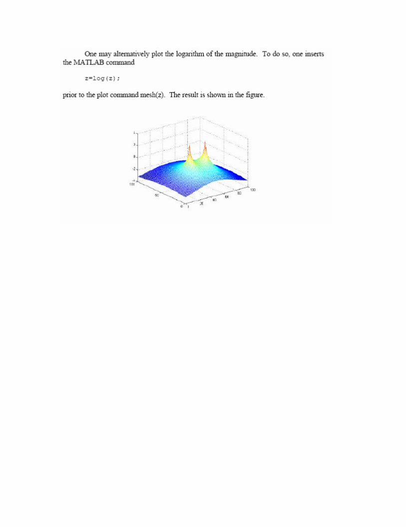
1. 3-d Plots and Bode. A system has transfer function 134

3)( 2 +++

=ss

ssH

a. Use MATLAB to make a 3-D plot of the magnitude of H(s) b. Use MATLAB to make a 3-D plot of the phase of H(s) c. Use MATLAB to draw mag and phase Bode plots

2. Bode. A system has transfer function

)250)(1002(

)50)(1()( 2 +++++

=ssss

sssH .

a. Plot Bode mag and phase roughly by hand using the Rules of Thumb. b. Use MATLAB to plot Bode mag and phase.

3. Bode Design. A transfer function is given by)6)(2(

24)(++

=sss

sH , this is a system

with a pole at origin and couple of stable poles. A compensator aircraft is selected:

Where .404)( ⎟⎠⎞

⎜⎝⎛

++

=ssksK

a. Draw Bode magnitude and phase plot for open loop system. b. Calculate gain margin and phase margin for open loop system. c. Draw Bode magnitude and phase plot for the compensator alone. d. Draw Bode magnitude and phase plot for the closed loop system when k=10. e. Calculate gain margin and phase margin of the closed loop system with a

discussion on system stability. f. Is it possible to find a value of k that yields a phase margin of 500 ? g. Find system’s step response for this value of k.

12