EE 201 Lecture Notes - METU EEEeee.metu.edu.tr/.../EE201/EE201_Fall201112/lecture_notes/2ndorder.pdf · EE 201 Lecture Notes ... damental for the analysis of linear time-invariant

EE 201 Lecture Notes

Cagatay CandanElectrical and Electronics Engineering Dept.

METU, Ankara.

Draft date January 13, 2013

Chapter 1

Second Order Circuits

1.1 Introducing Second Order Circuits

An understanding of the second order circuits and their modes of operation is fun-damental for the analysis of linear time-invariant systems. The phrase “linear time-invariant system” appears frequently in the notes. We should note that this conceptis not only central to the electrical engineering, but also important for many otherengineering disciplines. In our curriculum, a sequence of courses introduces topicsrelated to linear system theory, such as the second order circuits. The first coursein this list is EE201. After EE201, there are some other mandatory courses (EE202,EE301, EE302) and a number of 4th year courses which are linked with the linearsystem theory.

The response of a linear time-invariant system, which can be circuit or a me-chanical system or any other dynamical system, can be interpreted as a joint actionof its “modes”. (The word mode will become clearer in this chapter.) The super-position of the modes comprise the overall reaction of the system. Specifically, thereaction of an unforced system (a system excited only by the initial conditions, i.e.no external input) is called the natural response. As the name implies this responseshows how the system behaves once it is energized at t = 0 and then left on its own(no external input or forcing term for t > 0). In many applications, you may not bepleased with the way the system behaves and you inject an input to steer the systemto a desirable direction. Then the next question is what should be the input to steerthe system towards the desired direction. To do that we need to understand thehow the system reacts to the external inputs. This chapter presents some answers

1

2 CHAPTER 1. SECOND ORDER CIRCUITS

to such questions. In this chapter, the second order circuits are used to illustratethe answers of such questions.

If we go back to the first order circuits, the first order circuits have a singlemode, that is a single way of reacting to a given initial condition. This mode ischaracterized by an exponential decay and we know that the decay rate is relatedto the time-constant of the system.

The second order circuits have two modes and the analysis is a little bit moreintricate. As a side note, we would like to mention that the first order and sec-ond order systems are fundamental for the analysis of N’th order systems, since ahigher order system can be decomposed as a cascade of first and second order sys-tems. Hence, a through understanding of second order systems is important for theperception of the whole theory.

1.2 Parallel RLC Circuit

We present the main concepts through the parallel RLC circuit. The parallel andseries RLC circuits are classical circuits which are the duals of each other. Hence,their mathematical treatment is identical. We focus on the parallel RLC circuit inthis section and briefly examine the series RLC after the completion of this section.

Figure 1.1 shows the parallel RLC circuit configuration. We assume that thecircuit is energized with the initial conditions of VC(0

−) = V0 and IL(0−) = I0. The

goal is to analyze this circuit for t ≥ 0 under the external input of is(t) and also theinitial conditions.

Figure 1.1: Parallel RLC Circuit

We embark on the analysis by writing the KCL equation at the top node ofthe circuit:

−is(t) + IR(t) + IL(t) + iC(t) = 0

Using the component relations for R, L and C, this equation can be written asfollows:

1.2. PARALLEL RLC CIRCUIT 3

VC(t)

R︸︷︷︸IR(t)

+ IL(0−) +

1

L

∫ t

0−VC(τ)dτ︸︷︷︸

IL(t)

+Cd

dtVC(t)︸︷︷︸

ic(t)

= is(t), t > 0(1.1)

In the equation above, the initial condition for the inductor, IL(0−), is explicitly

present; but the initial condition for the capacitor, VC(0−), is absent. The equation

(1.1) and the initial condition VC(0−) = V0 (which is the initial condition absent in

the equation) forms the complete description of the system via an integro-differentialequation.

By taking the time-derivative of (1.1) for t > 0, the integro-differential equationis converted into a differential equation:

1

R

d

dtVC(t) +

1

LVC(t) + C

d2

dt2VC(t) =

d

dtis(t)(1.2)

The same equation can be written using the operator notation D∆= d

dtas follows:(

D2 +1

RCD +

1

LC

)VC(t) =

1

CD is(t)(1.3)

Note that after taking the derivative the initial condition for the inductor vanishes.Hence, we need two initial conditions to find the solution from the differential equa-tion.

We know that a differential equation is not complete unless its initial conditionsare specified. Since the differential equation above is with respect to VC(t), the initialconditions for VC(0

−) and VC(0−) should be provided. (The dot on top refers to the

derivative of the function.) We are already given the initial condition for VC(0−)

which is VC(0−) = V0; and we need to find the initial condition for VC(0

−). To findthat, we can examine, the t = 0− circuit.

The parallel RLC circuit at t = 0+ is shown in Figure 1.2. Note that, wehave replaced the inductor and capacitor in the circuit with the current and voltagesources, respectively. The equivalency of t = 0− and t = 0+ values is due to thecontinuity of these circuit variables for the bounded inputs and the replacement ofthe components for t = 0+ with the sources is possible by the substitution theorem.By inspection of Figure 1.2, the capacitor current at t = 0+ can be written as follows:

ic(0+) = C

d

dtVC(0

+) = −V0

R− I0 − is(0

+)(1.4)

The required initial condition is then ddtVC(0

+) = −(

V0

RC+ I0+is(0+)

C

). Now, we can

write the differential equation along with required initial conditions as follows:


R I0

At t = 0+

0

0

)0()0(

)0()0(

III

VVV

LL

CC

==

==+−

+−

is(0+)

ic(0+)

V0

Figure 1.2: Parallel RLC Circuit at t=0−

(D2 +

1

RCD +

1

LC

)VC(t) =

1

CD is(t) ,

VC(0+) = V0

VC(0+) = −

(V0

RC+ I0+is(0+)

C

)(1.5)

The last equation completely characterizes the system for t ≥ 0+. This means that itis possible to forget that the problem is a circuit analysis problem and work with thegiven differential equation in a purely mathematical manner and find the solutionVC(t).

The next task is the solution of the differential equation; but before that wepresent another description for the same circuit. From Figure (1.1), it is possible towrite the following two relations:

VC(t)

R+ IL(t) + C

d

dtVC(t) = is(t)

Ld

dtIL(t)︸︷︷︸

vL(t)

= VC(t)

We retain the differentiated variables on the left hand side and move all others tothe right hand side to get the following:

d

dtVC(t) = −VC(t)

RC− IL(t)

C+

is(t)

Cd

dtIL(t) =

1

LVC(t)

This equation can also be written using matrices. (The matrices are the essentialtools for the analysis of linear systems and can significantly ease the mathematicaltreatment of the topic. Don’t get intimidated by matrices, everyone gets, eventually,along very well with matrices!)

1.2. PARALLEL RLC CIRCUIT 5[VC(t)

IL(t)

]=

[− 1

RC− 1

C1L

0

] [VC(t)IL(t)

]+

[1C

0

]is(t)(1.6)

The equation system shown in (1.6) is a first order matrix differential equation.(Your differential equations teacher would be very happy if you can immediatelysay that the solution of such equations can be written in terms of eAt matrix!) Theinitial conditions to make this equation complete is VC(0

−) = V0 and IL(0−) = I0.

Note that, for bounded inputs, i.e. is(t) < M for some M , VC(0+) = VC(0

−) = V0

and IL(0−) = IL(0

+) = I0. Note that, there is no need to do a t = 0+ analysis, aswe did in Figure 1.2, to find the initial conditions.

Note that it is possible to retrieve the 2nd order scalar differential equationfor VC(t) given in (1.5) from the matrix differential equation given in (1.6). To dothat take the derivative of the first equation in (1.6) and substitute IL(t) with thesecond equation of (1.6). Once this is done, we get the scalar 2nd order differentialequation for VC(t). Hence, both representations are equivalent to each other, it ispossible to go back and forth between different representations.

We would like to note that it is possible to write the differential equation forany other circuit variable of the parallel RLC circuit. For example, to write anequation for IL(t), we can utilize (1.6). First write VC(t) and VC(t) in terms of IL(t)and IL(t). Then take the derivative of the second equation to get IL(t). Finally,replace all VC(t) and VC(t) appearing in IL(t) with the inductor current functions.This gives us an equation for IL(t). We can show these steps as follows:

d2

dt2IL(t) =

1

L

d

dtVc(t)

(1.6)=

1

L

(−VC(t)

RC− IL(t)

C

)(1.6)=

1

L

(−LIL(t)

RC− IL(t)

C

)

It is also possible write a second order differential equation for the resistorcurrent by noting that IR(t) = VC(t)/R or VC(t) = RIR(t). To write the describingequation for IR(t), you can replace VC(t) and its derivatives in (1.5) with IR(t) andIR(t).

Furthermore you can invent new circuit variables such as x(t) = VC(t) + IL(t)y(t) = VC(t)+2IL(t) and write the matrix differential equation satisfied by x(t) andy(t), or you may write the scalar 2nd order differential equation satisfied by x(t).(It may not be clear why you may want to do such a thing at this point.)

Hence there are many ways of describing the same circuit. All of these de-scriptions are inter-related and we can go back and forth between these equivalent


descriptions. (For experienced readers, we note that the natural frequencies of thecircuit, or the system poles or the eigenvalues of the A matrix is identically the samefor every representation. If you do not understand this parenthesis, don’t worry!)

1.2.1 Zero-Input Solution

The zero-input solution characterizes the natural response of the circuit. In otherwords, the zero-input solution is the solution when the circuit is energized at t = 0−

and then left on this own (no external forcing). The question is to find the variationof the circuit variables or the evolution of the circuit variables under the KVL andKCL constraints, given the initial conditions. Stated differently the question is whatis happening in the circuit due to the initial conditions in the absence of externalinput.

Figure 1.3: Zero-Input Parallel RLC Circuit

The defining equation: In resistive LTI circuits, the equation defining thesolution of the circuit is a linear equation system. As we have noted before, thenumber of unknowns for such a description can be the number of nodes or the numberof meshes. For resistive circuits with non-linear elements, the defining equationsystem is a non-linear equation. The non-linear relation is a quadratic equation ifwe have component with the relation V = i2R.

The defining equation for dynamic circuits can be an integro-differential equa-tion as we have noted in (1.1). The integral equations have certain advantages interms of computation and there is a strong mathematical theory for the integralequations. In this course we prefer the differential equations descriptions for whichthere is an equally strong theory. (The differential equations can be more funda-mental in equation writing since they describe the behaviour of the system via localdifferences.) The differential equation describing the circuit given in Figure 1.3 isgiven in (1.5) and reproduced below:(

D2 +1

RCD +

1

LC

)VC(t) =

1

CD is(t) , with

VC(0+) = V0

VC(0+) = −

(V0

RC+ I0+is(0+)

C

)When the input is(t) = 0 (zero-input), the equation characterizing the zero-input


solution is:(D2 +

1

RCD +

1

LC

)VC(t) = 0, with

VC(0+) = V0

VC(0+) = −

(V0

RC+ I0

C

)(1.7)

We present the general solution for the following differential equation:(D2 + 2αD + ω2

o

)VC(t) = 0(1.8)

We make the following guess for the solution:

Vc(t) = ceλt

If this function is indeed the solution, then the differential equation (1.7) should besatisfied for all t > 0. To check the guess, we insert the function into the differentialequation and get the following equation:

c(λ2 + 2αλ+ ω2o) = 0(1.9)

The last equation shows that the guess is correct if c = 0 or λ2+2αλ+ω2o = 0. The

solution c = 0 becomes VC(t) = 0 which can not be the right solution the unlessall initial conditions are zero. Thus, the non-trivial solutions should have λ whichsatisfies:

(λ2 + 2αλ+ ω2o) = 0(1.10)

This equation is called the characteristic equation of the system. The roots of thecharacteristic equation are called the natural frequencies. The roots can be writtenas follows:

Natural Frequencies: λ1,2 = −α±√

α2 − ω2o(1.11)

The solution for the zero-input can then be written as follows:

VC(t) = c1eλ1t + c2e

λ2t, t ≥ 0(1.12)

where λ1 and λ2 are the natural frequencies and c1 and c2 are the arbitrary constants.(The constants c1 and c2 are set to meet the initial conditions at t = 0+.)

Types of Zero-Input Responses: The zero-input responses are categorizedby the natural frequencies, that is the roots of the characteristics equation given in(1.10) determine the type of response.

The possibilities for the roots are:

i. Distinct real roots (∆ > 0, i.e α > ωo)


ii. Repeated real roots (∆ = 0, i.e. α = ωo)

iii. Complex conjugate roots (∆ < 0, i.e. α < ωo)

The parameter ∆ is the discrimant value of the quadratic given in (1.10), ∆ =4(α2 − ω2

o). Each one of these possibilities listed is attributed as a circuit response.

Before the discussion of the responses, we need to introduce some terminologyfor the parameters α and ωo appearing in (1.10). The parameter α, which is 1/(RC)for the parallel RLC circuit, is called the damping factor. The parameter ωo, whichis 1/

√LC for the parallel RLC, is called the resonance frequency.

Parallel RLC :

α = 1

2RC

ωo =1√LC

The terminology will become more apparent with the introduced topics.

Characteristic Equation:λ2 + 2αλ+ ω2

o = 0

α : Damping factor (1/sec, Hz.)ωo : Natural frequency (1/sec, Hz.)

i. Overdamped Circuits (α > ωo): The natural frequencies for the over-damped circuits are real valued and distinct.

For the parallel RLC circuit with R = 1/5 Ω, L = 1/8 H and C = 1/2 F, wehave α = 5 and ωo = 4. Since α > ωo, the response is overdamped, i.e. damping isgreater than than ωo. The characteristic equation for this circuit is λ2+10λ+16 = 0and the natural frequencies are λ = −8,−2. The zero-input solution is then

V ziC (t) = c1e

−2t + c2e−8t, t ≥ 0.

The constants c1 and c2 are to be determined according to the initial conditions att = 0+.

ii. Critically Damped Circuits (α = ωo): The natural frequencies forcritically damped circuits are real valued and repeated.

Let’s take R = 1/4 Ω, L = 1/8 H and C = 1/2 F, then α = ωo = 4 and thecharacteristic equation is λ2 + 8λ + 16 = 0. The natural frequencies are λ = −4.The zero-input solution is then

V ziC (t) = c1e

−4t + c2te−4t, t ≥ 0.


iii. Underdamped Circuits (α < ωo): The natural frequencies for criticallydamped circuits are complex valued and two natural frequencies are the complexconjugates of each other.

Let’s take R = 1/3 Ω, L = 1/8 H and C = 1/2 F in the parallel RLC circuit,then α = 3 and ωo = 4. It is clear that the damping coefficient smaller than the nat-ural frequency, hence the name underdamped. The characteristic equation for thissystem is λ2 + 6λ + 16 = 0. The natural frequencies are λ = −3 + j

√7,−3− j

√7.

The zero-input solution is then:

V ziC (t) = c1e

(−3−j√7)t + c2te

(−3+j√7)t, t ≥ 0

The solution for this case is complex valued. It may not be clear from this repre-sentation that the solution we get is a reasonable solution representing the physicsof the problem, that is if the solution is complex valued, it would be very hard forus to interpret as the capacitor voltage! Luckily, as it is shown belown, there areno such interpretation problems and the theory extends smoothly towards complexvalued natural frequencies.

Let’s assume that VC(0+) and VC(0

+) values are provided. Then to find V ziC (t),

we need to set c1 and c2 appearing in (1.13) to meet the initial conditions at t = 0+.

VC(0+) = c1 + c2

VC(0+) = λ1c1 + λ2c2(1.13)

Here λ1 and λ2 are complex valued natural frequencies, which is λ1 = (−3 − j√7)

and λ2 = (−3 + j√7) for the presented example.

The claim is that if VC(0+) and VC(0

+) are real valued, then c1 = c∗2 (c1 andc2 are complex conjugates of each other). To show this claim, we take the complexconjugate of the equations in (1.13), the resultant equation is as follows:

VC(0+) = c∗1 + c∗2

VC(0+) = λ∗

1c∗1 + λ∗

2c∗2

But since λ1 and λ2 are complex conjugates of each other, the equation systemreduces to:

VC(0+) = c∗2 + c∗1

VC(0+) = λ1c

∗2 + λ2c

∗1(1.14)

Now we compare (1.13) and (1.14). If the equation system given in (1.13) has aunique solution (which is the case, think about why?), then that solution for (1.13)


should be solution of (1.14). Due to the uniqueness of the solution, we have c1 = c∗2and c2 = c∗1. This shows that the claim is indeed correct.

Going back to (1.13), we can now write the zero-input solution for t > 0 as

V ziC (t) = c1e

λ1t + c2eλ2t

(a)= c1e

λ1t + c∗1eλ∗1t

(b)= 2Re

c1e

λ1t

(c)= 2Re

||c1||ej]c1eλ1t

= 2||c1||Re

ej]c1eλ1t

(d)= 2||c1||Re

ej]c1e(λ

r1+jλi

1)t

= 2||c1||Reeλ

r1tej(λ

i1t+]c1)

(e)= 2||c1||eλ

r1tRe

ej(λ

i1t+]c1)

(f)= 2||c1||eλ

r1t cos(λi

1t+ ]c1)(g)= d1e

λr1t cos(λi

1t+ d2)

In line (a): The complex conjugacy relation between the parameters is used.In line (b): Summation of a function and its complex conjugate yields two times thereal part of the function.In line (c): The constant c1 is expressed in polar coordinates.In line (d): The constant λ1 is expressed as λ1 = λr

1 + jλi1.

In line (e): The real valued function eλr1t is pulled out of the real operator.

In line (f): Euler’s formula.In line (g): Undetermined constants are replaced with a new set of undeterminedconstants d1 and d2.

If we go back to the parallel RLC circuit example, the zero-input is then

V ziC (t) = d1e

−3t cos(√7t+ d2), t ≥ 0

Again note that by selecting d1 and d2, it is possible to meet any given initialcondition at t = 0+.

Comparison of Under/Critical and Overdamped Responses:

(to be written...)


1.2.2 Zero-State Solution

The zero-state solution assumes the circuit is not energized initially, that is theinitial voltage of all capacitors and the initial current of all inductors are zero. Thezero-stage solution is the response due to the applied input in the absence of anyinitial conditions, that is when the system is at rest initially.

The general approach is as follows:

i. Find the initial conditions at t = 0+ by inspecting the t = 0+ circuit.

ii. Solve the differential equation for t > 0 with the t = 0+ initial conditions.

For the zero-state solution, the circuit is initially at rest; therefore t = 0− valuesfor the capacitor voltages and inductor currents are zero. From our earlier discus-sions, we know that the capacitor voltages and inductor currents is a continuousfunction of time if the input is bounded. As discussed before, this is a consequenceof the terminal equations for the capacitor (VC(t) = VC(0)+1/C

∫ t

0IC(t

′)dt′) and the

inductor (IL(t) = IL(0)+1/L∫ t

0VL(t

′)dt′). Therefore, if there is no impulsive sourcein the circuit, VC(0

+) = VC(0−) and IL(0

+) = IL(0−) is granted. The continuity of

the VC(t) and IL(t) is the golden rule that should always be remembered.

Below we find the zero-state response to ramp, unit step and impulse input.The method shown below can also be used to directly write the complete solution,i.e. solving a circuit without zero-input and zero-state decomposition. As we havediscussed before, this decomposition enables us to apply the superposition for thezero-stage responses. Therefore it is very useful if we have a superposition of elemen-tary functions at the input. In this case, the zero-state response to the superposedinput is the superposition of zero-state responses to each input. This is the reason(the possibility of superposition) that makes the zero-state responses important tous.

i. Ramp Response: Figure 1.4 shows the circuit at t = 0+ when the inputis the ramp function.

An inspection of this circuit, reveals that all circuit variables in this currenthas the value of zero t = 0+, that is IC(0

+) = 0 and therefore VC(0+) = 0. Hence

the t = 0+ initial conditions for the ramp input is VC(0+) = VC(0

+) = 0 and thefirst step of the procedure given above is completed.

The differential equation for the ramp input, i.e. is(t) = r(t) is as follows:(D2 +

1

RCD +

1

LC

)VC(t) =

1

CD is(t) =

1

Cu(t),

VC(0+) = 0

VC(0+) = 0

For t > 0, the differential equation is


R I0 V0

At t = 0+

0)0(

0)0(

0

0

==

==−

−

II

VV

L

C

is(0+)

+

VL

-

R

At t = 0+

)0()0(

)0()0(

0)0()0(

++

++

++

=

=

==

LL

CC

s

ILV

VCI

ri

&

&

is(0+)

+

VL

- Ic

Figure 1.4: At t = 0+ circuit for the ramp input(D2 +

1

RCD +

1

LC

)VC(t) =

1

C, t > 0

The zero-state solution is then

V zsC (t) = L+ c1e

λ1t + c2eλ2t, t > 0

Here λ1, λ2 are the natural frequencies and the constants c1, c2 should be selectedthe meet the initial conditions at t = 0+.

ii. Step Response: Figure 1.5 shows the circuit at t = 0+ when the input isthe step function.

R I0 V0

At t = 0+

0)0(

0)0(

0

0

==

==−

−

II

VV

L

C

is(0+)

+

VL

-

R

At t = 0+

)0()0(

)0()0(

1)0()0(

++

++

++

=

=

==

LL

CC

s

ILV

VCI

ui

&

&

is(0+)

+

VL

- Ic

Figure 1.5: At t = 0+ circuit for the unit step input

A simple analysis of the t = 0+ which does not contain any dynamic elements,but only sources and resistors reveals that VC(0

+) = 0 and VC(0+) = 1/C. It

should be noted that VC(0+) is due to the continuity of the capacitor voltage for the

bounded inputs (the golden rule!) and does not follow from any analysis.

Then the differential equation for the unit step input, i.e. is(t) = u(t) is asfollows:

1.2. PARALLEL RLC CIRCUIT 13(D2 +

1

RCD +

1

LC

)VC(t) =

1

CD is(t) =

1

Cδ(t),

VC(0+) = 0

VC(0+) = 1/C

(1.15)

On the right hand side of the differential equation we have a δ(t) functionwhich is quite a problem if we were presented with such a differential equation at adifferential equations course; but note that for t > 0, the differential equation is(

D2 +1

RCD +

1

LC

)VC(t) = 0, t > 0

The zero-state solution for t > 0, is then

V zsC (t) = c1e

λ1t + c2eλ2t, t > 0

Here λ1, λ2 are the natural frequencies and the constants c1, c2 should be selectedthe meet the initial conditions at t = 0+.

iii. Impulse Response: Figure 1.6 shows the circuit that is be analyzed forVC(0

+) and VC(0+) values.

)(tδ R

0-<t< 0+

+

VL

- Ic

R I0

At t = 0+

+

VL

-

V0

)0()0(

)0()0(++

++

=

=

LL

CC

ILV

VCI

&

&

)(tδ R

0-<t< 0+

+

VL

- Ic

R I0

At t = 0+

+

VL

-

V0

)0()0(

)0()0(++

++

=

=

LL

CC

ILV

VCI

&

&

R

0-<t< 0+

+

VL

- Ic

R I0

At t = 0+

+

VL

-

V0

)0()0(

)0()0(++

++

=

=

LL

CC

ILV

VCI

&

&

Figure 1.6: At t = 0+ circuit for the impulse input

The input is not a bounded one, therefore we can not apply the rule statingthat the capacitor voltage and inductor current is continuous. The circuit on the leftside of Figure 1.6 shows that IC(t) = δ(t) “during the application of the impulse”.

Hence VC(0+) = VC(0

−) + 1/C∫ 0+

0−ic(t

′)dt′ = 1/C. How about IL(0+)? To find

IL(0+), we need to find VL(t) during the application of the impulse. It can be noted

from Figure 1.6 that VL(t) = 0 in between 0− and 0+ and hence IL(0+) = 0.

To solve the differential equation written for VC(t), we need the initial condi-tions for VC at t = 0+. To find VC(0

+), we examine t = 0+ circuit, which is thecircuit just after the application of the impulse. This circuit is given on the rightside of Figure 1.6. In this circuit V0 = 1/C and I0 = 0. Then a resistive circuitanalysis reveals that IC(0

+) = −VC(0+)/R = −1/(RC), then VC(0+) = −1/(RC2).

We are done with the finding of the initial conditions.


The differential equation for the unit impulse input, i.e. is(t) = δ(t) is asfollows:(

D2 +1

RCD +

1

LC

)VC(t) =

1

CD is(t) =

1

Cδ(t),

VC(0+) = 1/C

VC(0+) = −1/RC2

On the right hand side of the differential equation, we have the derivative ofthe δ(t) function which is called the doublet function. (A rigorous solution of adifferential equation with the impulse input and its derivatives requires familiaritywith the generalized functions. A semi-rigorous but convincing method of solutionis presented as an appendix to this chapter.) The function δ(t) on the right handside of the differential equations can cause nervousness and nausea to some readers,but readers should be assured that for t > 0, the differential equation reduces to(

D2 +1

RCD +

1

LC

)VC(t) = 0, t > 0

The zero-state solution for t > 0, is then

V zsC (t) = c1e

λ1t + c2eλ2t, t > 0

Here λ1, λ2 are the natural frequencies as before and the constants c1, c2 should beselected the meet the initial conditions at t = 0+.

Remark #1: We would like to note that the solution of the differential equa-tions with a forcing term of δ(t) (and its derivatives) is not a straightforward prob-lem. The technique presented in this chapter passes the difficulties associated withthe impulse by analyzing t = 0+ circuit. A time-domain verification of the t = 0+

circuit analysis result using differential equations knowledge (no circuit theory) re-quires fairly sophisticated mathematical analysis knowledge. Another approach forthe solution of such differential equations is the transform domain methods, i.e.the Laplace domain, which is throughly presented in EE202 within the context ofs-domain circuit analysis.

Remark #2: As noted before instead of having a 2nd order scalar differen-tial equation for VC(t), we may write a 1st order matrix differential equation forVC(t) and IL(t). Both equations characterize the same circuit and their solution isidentical. It should always be remembered that alternative characterizations canbe always useful i.) to justify your solution and ii.) to find alternative methodsto reach the same solution. In many problems the method to the solution can bemore critical and lead to a better conceptual understanding and generalizations ofthe problem in hand.

The 1st order matrix differential equations present an alternative method forcircuit characterization. In EE202, this topic is investigated under the heading of


state equations. The state equations have a number of advantages in comparison toscalar differential equations.

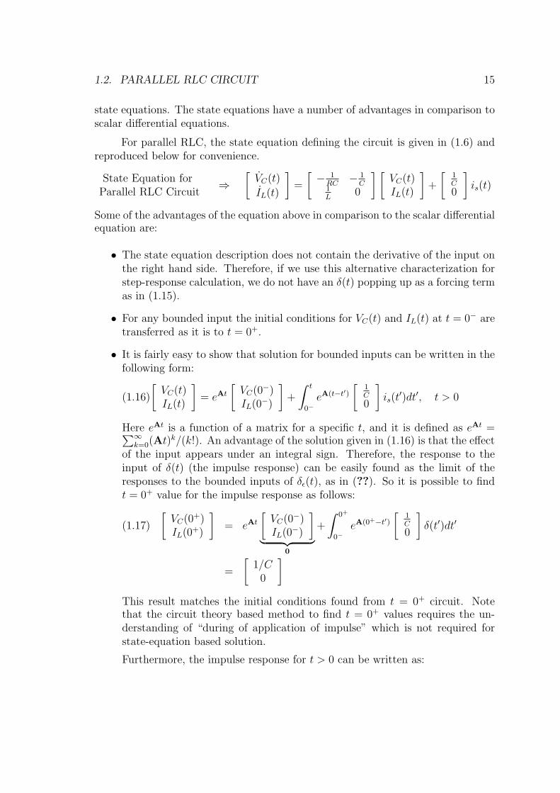
For parallel RLC, the state equation defining the circuit is given in (1.6) andreproduced below for convenience.

State Equation forParallel RLC Circuit

⇒[VC(t)

IL(t)

]=

[− 1

RC− 1

C1L

0

] [VC(t)IL(t)

]+

[1C

0

]is(t)

Some of the advantages of the equation above in comparison to the scalar differentialequation are:

• The state equation description does not contain the derivative of the input onthe right hand side. Therefore, if we use this alternative characterization forstep-response calculation, we do not have an δ(t) popping up as a forcing termas in (1.15).

• For any bounded input the initial conditions for VC(t) and IL(t) at t = 0− aretransferred as it is to t = 0+.

• It is fairly easy to show that solution for bounded inputs can be written in thefollowing form:[

VC(t)IL(t)

]= eAt

[VC(0

−)IL(0

−)

]+

∫ t

0−eA(t−t′)

[1C

0

]is(t

′)dt′, t > 0(1.16)

Here eAt is a function of a matrix for a specific t, and it is defined as eAt =∑∞k=0(At)k/(k!). An advantage of the solution given in (1.16) is that the effect

of the input appears under an integral sign. Therefore, the response to theinput of δ(t) (the impulse response) can be easily found as the limit of theresponses to the bounded inputs of δϵ(t), as in (??). So it is possible to findt = 0+ value for the impulse response as follows:[

VC(0+)

IL(0+)

]= eAt

[VC(0

−)IL(0

−)

]︸︷︷︸

0

+

∫ 0+

0−eA(0+−t′)

[1C

0

]δ(t′)dt′(1.17)

=

[1/C0

]This result matches the initial conditions found from t = 0+ circuit. Notethat the circuit theory based method to find t = 0+ values requires the un-derstanding of “during of application of impulse” which is not required forstate-equation based solution.

Furthermore, the impulse response for t > 0 can be written as:

16 CHAPTER 1. SECOND ORDER CIRCUITS[VC(t)IL(t)

]= eAt

[VC(0

+)IL(0

+)

]+

∫ t

0+eA(t−t′)

[1C

0

]δ(t′)︸︷︷︸

0

dt′

= eAt

[VC(0

+)IL(0

+)

]= eAt

[1/C0

], t ≥ 0

This shows that the impulse response for VC(t) and IL(t) can be found bymultiplying eAt matrix and b = [1/C, 0]T vector. This result is valid forany circuit having state variables listed in x(t) vector and state equation ofx(t) = Ax(t) + b is(t).

Remark #3: (A Mechanical Analogy) To illustrate the differences in be-tween the overdamped and underdamped responses, we present a mechanical analogfor the parallel RLC circuit. The mechanical analogy carries our everyday intuitionof dynamical systems to the RLC circuits.

M

x=0x

Figure 1.7: Mechanical Analog of 2nd Order RLC circuit

Figure 1.7 shows a mass M attached to a linear spring with the spring constantk on a rough surface with friction. We assume that the system is energized at t = 0−

and released at t = 0. There is no external force on the system for t > 0. Our goalis to analyze what happens after we release.

We assume that the origin of the selected coordinate system coincides withthe equilibrium position of the mechanical system. In other words when the massis at x = 0, the spring is not compressed, i.e. the force exerted by the spring on themass is zero. The position of the mass is denoted by the function x(t). Our goal isto find x(t) for t > 0.

The initial energy can be deposited to the mechanical system in two ways.The mass can have a non-zero initial speed or the spring can be initially compressed.


Mass with a non-zero speed at t = 0− leads to the storage of kinetic energy, 12Mx2(t).

Initially compressed spring leads to the storage of the potential energy, 12kx2(t). The

initial rest conditions (no initial energy) for the mechanical system is then x(0−) = 0,x(0−) = 0.

The analogy with the RLC circuit can be established by noting that the storedelectrical energy in the circuit at time t is 1

2CVC(t)

2 and the stored magnetic energyis 1

2LIL(t)

2. For the parallel RLC circuit, if we choose to denote IL(t) as x(t), thenx(t) = VC(t)/L. Hence the electrical and magnetic energy at time t can be writtenas 1

2CL2x(t)

2 and 12Lx(t)2 respectively. It should be noted that the energy relations

for the electrical and mechanical systems are closely related. (Note that by settingthe mass as M = C/L2 and spring constant k as L, we can reproduce the samefunctional relations for mechanical and electrical systems. It should be noted ourgoal in making this analogy is to understand the differences between underdampedand overdamped responses, not the construction of an exact mechanical analog of anelectrical circuit. Therefore attention should not be focused on the arbitrary systemconstants such as M,k or R,L,C; but we should focus on the functional relations.)

By Newton’s axioms, we can write that Fnet = m d2

dt2x(t) and for the particular

mechanical system Fnet = −kx(t)−µx(t). In the last equation µx(t) is the force dueto friction. (In Physics 105, the friction force is, in general, denoted as µ. Here weassume that the friction force is proportional to velocity of the object. The frictionused in this model is the viscous friction which is the friction faced by a movingobject in a liquid or gas. Figure 1.7 does not explicit show the type of friction. Ifyou want, you may consider that the object M is floating on the surface of a poolfilled with some fluid.)

The governing equation for the position of the mass is as follows:

Md2

dt2x(t) + µ

d

dtx(t) + kx(t) = 0, with

x(0−) = X0

x(0−) = X0

The same equation can be written in the standard form as shown below:

d2

dt2x(t) +

µ

M︸︷︷︸2α

d

dtx(t) +

k

M︸︷︷︸ω20

x(t) = 0, withx(0−) = X0

x(0−) = X0

From the last equation, we can note the damping factor and resonant frequencyconstants of the system, α = µ/2M and ω2

o = k/M . (Note that if M = C,k =1/L,µ = 1/R, α = R/2C and ω2

o = 1/LC exactly matching the differential equationof the parallel RLC circuit given in (1.7).) Note that the friction only effects dampingcoefficient and it is analogous to R in the RLC circuit in this sense.


Underdamped Case (µ is small): When µ is sufficiently small α < ω0

and the mechanical system will be underdamped. The word “underdamped” isspecifically chosen to imply that the damping (or the friction force) is small orbelow a certain threshold for this case. The response for this case is in the form:

x(t) = d1eλr1t cos(λi

1t+ d2)

where d1 and d2 are chosen to satisfy the initial conditions and λr1 and λi

1 are thereal and imaginary parts of the natural frequency λ1.

The most important observation about this solution is that x(t) changes itssign infinitely many times until it comes to a final rest In other words, the objectcrosses the equilibrium point (x = 0) and proceeds towards, say, the positive x-axis.After some time, the object slows down (x(t) is negative valued) and then stopstemporarily (when x(t) = 0, note that when it stops it stretches/compresses thespring to the maximum level and at this instant kinetic energy is zero) and thenspeeds up in the opposite direction that is towards negative x-axis direction. Aftersome time, it crosses the equilibrium point and slows down due to the compressionof the spring (storage of potential energy). Then stops and repeats the some motion.At every oscillation cycle, the system losses some part of its energy due to friction.Because of this, it can never attain the level of spring compression/streching that ithas achieved in the earlier cycles. The object is said have decaying oscillations.

Now, read the previous paragraph with the following replacements: Mass →Capacitor; Inductor → Spring; Friction → Conductance (1/R, i.e. no friction R →∞); Kinetic Energy → Electrical Energy; Potential Energy → Magnetic Energy.

The important conclusion is, one more time, that the underdamped systemsdue to small friction (or small ohmic losses) oscillates around the equilibrium pointand eventually comes to a stop.

Overdamped Case (µ is large): When µ is sufficiently large α > ω0 and themechanical system will be overdamped. The response for this case is in the form:

x(t) = c1eλ1t + c2e

λ2t

Here λ1, λ2 are the distinct and negative valued real numbers which are the naturalfrequencies of the system. The parameters c1, c2 are, as before, chosen to satisfy theinitial conditions.

In this case the response does not have oscillations across the equilibriumpoint. The response is the summation of two monotonic functions. You can showthat depending on the initial conditions, the response either have a single equilibriumcrossing (only one sign change) or no equilibrium crossings (x(t) keeps its sign, thatis remains positive or negative and monotonically approaches the equilibrium state

1.3. SERIES RLC CIRCUIT 19

of x(t) = 0). In both cases, system reaches the equilibrium point via an exponentialdecay.

Note that the presence or absence of oscillations is determined by the dampingfactor which is directly influenced by the amount of friction (or resistance) in thesystem. Again note that, the type of the response is the property of the system, notits initial conditions or external input.

Lossless Case (µ = 0): When µ is equal to zero, there is no friction in thesystem and the mechanical system has sustained oscillations. In other words theobject moves back and forth across the equilibrium point. The solution in this caseis

x(t) = d1 cos(λi1t+ d2)

where λ1,2 = ±j ωo. For the lossless case, the oscillation frequency is the resonancefrequency ωo. The object moves back and forth across x = 0 point, ωo times atevery 2π seconds.

Remark #4: The topic of second order circuits is also examined under thetopic of frequency response in EE202. Especially the underdamped case will bebrought under scrutiny for the description of RLC resonators.

1.3 Series RLC Circuit

The series RLC circuit is the dual of the parallel RLC circuit. The circuit is shownin Figure 1.8.

Figure 1.8: Series RLC Circuit

We can write the differential equation characterizing the circuit as follows:

VR(t) + VL(t) + VC(t) = vs(t)

RIL(t) + Ld

dtIL(t) + VC(0

−) +1

C

∫ t

0−IL(t

′)dt′ = vs(t), t ≥ 0


By taking the derivative of the last relation, we can get the following differentialequation: (

D2 +R

LD +

1

LC

)IL(t) =

1

LDvs(t), t ≥ 0(1.18)

Note that, the differential equation given above can be written by noting the dualityof the parallel RLC and series RLC circuit. To do that one needs to replace R →1/R, L → C, C → L and VC(t) → IL(t), is(t) → Vs(t) in (1.3).

The differential equation for VC(t) can be written by noting that IL(t) =CDVC(t) for the series RLC circuit. By substituting CDVC(t) for IL(t) in(1.18), we get: (

D2 +R

LD +

1

LC

)CDVC(t) =

1

LDvs(t)

After the cancellation of D operator, we get the differential equation for VC(t):(D2 +

R

LD +

1

LC

)VC(t) =

1

LCvs(t)(1.19)

The only difference between the parallel and series RLC circuits as the definitionof damping factor and resonant frequency. All results and conclusions given for theparallel RLC is equally applicable to the series RLC circuit.

1.4 Examples

Example 1.1 Find VC(t) for t ≥ 0. The initial conditions are VC(0−) = −3 V and

IL(0−) = 0 A.

Figure 1.9: Example 1.1

Solution:

1.4. EXAMPLES 21

The differential equation for VC(t) has been previously given in (1.19). Once thegiven R,L and C values are substituted, we get:(

D2 + 10D + 16)VC(t) = 16vs(t)

We use zero-input and zero-state decomposition of the circuit to find the completesolution for VC(t).

Zero-Input Solution:

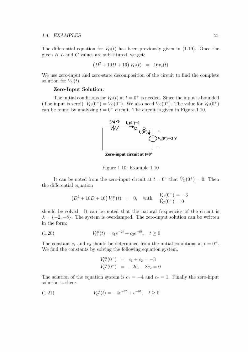
The initial conditions for VC(t) at t = 0+ is needed. Since the input is bounded(The input is zero!), VC(0

+) = VC(0−). We also need VC(0

+). The value for VC(0+)

can be found by analyzing t = 0+ circuit. The circuit is given in Figure 1.10.

5/4 Ω+

Vc(0+)=-3 V

-

IL(0+)=0

Ic(0+)

Zero-input circuit at t=0+

Figure 1.10: Example 1.10

It can be noted from the zero-input circuit at t = 0+ that VC(0+) = 0. Then

the differential equation(D2 + 10D + 16

)V ziC (t) = 0, with

VC(0+) = −3

VC(0+) = 0

should be solved. It can be noted that the natural frequencies of the circuit isλ = −2,−8. The system is overdamped. The zero-input solution can be writtenin the form:

V ziC (t) = c1e

−2t + c2e−8t, t ≥ 0(1.20)

The constant c1 and c2 should be determined from the initial conditions at t = 0+.We find the constants by solving the following equation system.

V ziC (0+) = c1 + c2 = −3

V ziC (0+) = −2c1 − 8c2 = 0

The solution of the equation system is c1 = −4 and c2 = 1. Finally the zero-inputsolution is then:

V ziC (t) = −4e−2t + e−8t, t ≥ 0(1.21)


Zero-State Solution:

The external input vs(t) can be written as follows:

vs(t) = 15 (u(t)− u(t− 30)) + δ(t− 35)

The zero-state response to this input is then

V zsC (t) = 15

(V stepC (t)− V step

C (t− 30))+ V impulse

C (t− 35)

The superposition of the zero-state responses is the main reason that we decomposethe solution into zero-input and zero-state parts. By calculating the step-responseand impulse response of series RLC circuit (which are the standard responses), it ispossible to present a solution to a fairly complicated input given in this example.

Step-Response: Like all zero-state responses, the initial conditions at t = 0−

are all zero. The circuit is not energized at t = 0−. Since the input is bounded,(the input is unit step function); VC(0

−) and IL(0−) values are transferred as it is to

t = 0+ values. Then VC(0+) = 0 and IL(0

+) = 0 and we do a t = 0+ to find VC(0+).

5/4 Ω IL(0+)=0

Ic(0+)

Zero-state response for unit step input, t=0+

u(0+)=1

Figure 1.11: Step response calculation, t = 0+

Figure 1.11 shows that VC(0+) = 0. Then the differential equation for the step

input is then(D2 + 10D + 16

)V zsC (t) = 16u(t), with

VC(0+) = 0

VC(0+) = 0

The solution for the step input is then:

V zsC (t) = 1 + d1e

−2t + d2e−8t, t ≥ 0

Again d1 and d2 are constants to be determined from t = 0+ initial conditions.These constants can be found as d1 = −4/3 and d2 = 1/3. Then the step responsecan be written as follows:

1.4. EXAMPLES 23

V stepC (t) = 1− 4

3e−2t +

1

3e−8t, t ≥ 0

Impulse-Response: The impulse response can be calculated by finding theinitial conditions at t = 0+ and then solving the differential equations for t > 0.Even though, this is possible; we use the knowledge that the impulse response is thederivative of the step response and immediately write the response as:

V impulseC (t) =

d

dtV stepC (t)

=8

3

(e−2t − e−8t

), t ≥ 0

Complete Solution: The solution can be written as the summation of thezero-input and the zero-state solutions which is

VC(t) = V ziC (t) + V zs

C (t)

=(−4e−2t + e−8t

)+ 15(V step

C (t)− V stepC (t− 30)) + 35V impulse

C (t− 35), t ≥ 0

This concludes the example.

...(to be continued, January 13, 2013)

Documents

EE 201 Lecture Notes - METU EEEeee.metu.edu.tr/.../EE201/EE201_Fall201112/lecture_notes/2ndorder.pdf · EE 201 Lecture Notes ... damental for the analysis of linear time-invariant