Educational Modeling for Fault Analysis of Power Systems

University of New Orleans University of New Orleans

ScholarWorks@UNO ScholarWorks@UNO

University of New Orleans Theses and Dissertations Dissertations and Theses

Fall 12-18-2014

Educational Modeling for Fault Analysis of Power Systems with Educational Modeling for Fault Analysis of Power Systems with

STATCOM Controllers using Simulink STATCOM Controllers using Simulink

Tetiana Brockhoeft University of New Orleans, [email protected]

Follow this and additional works at: https://scholarworks.uno.edu/td

Part of the Power and Energy Commons

Recommended Citation Recommended Citation Brockhoeft, Tetiana, "Educational Modeling for Fault Analysis of Power Systems with STATCOM Controllers using Simulink" (2014). University of New Orleans Theses and Dissertations. 1906. https://scholarworks.uno.edu/td/1906

This Thesis is protected by copyright and/or related rights. It has been brought to you by ScholarWorks@UNO with permission from the rights-holder(s). You are free to use this Thesis in any way that is permitted by the copyright and related rights legislation that applies to your use. For other uses you need to obtain permission from the rights-holder(s) directly, unless additional rights are indicated by a Creative Commons license in the record and/or on the work itself. This Thesis has been accepted for inclusion in University of New Orleans Theses and Dissertations by an authorized administrator of ScholarWorks@UNO. For more information, please contact [email protected].

https://scholarworks.uno.edu/

https://scholarworks.uno.edu/td

https://scholarworks.uno.edu/td

https://scholarworks.uno.edu/etds

https://scholarworks.uno.edu/td?utm_source=scholarworks.uno.edu%2Ftd%2F1906&utm_medium=PDF&utm_campaign=PDFCoverPages

http://network.bepress.com/hgg/discipline/274?utm_source=scholarworks.uno.edu%2Ftd%2F1906&utm_medium=PDF&utm_campaign=PDFCoverPages

https://scholarworks.uno.edu/td/1906?utm_source=scholarworks.uno.edu%2Ftd%2F1906&utm_medium=PDF&utm_campaign=PDFCoverPages

mailto:[email protected]

Educational Modeling for Fault Analysis of Power Systems

With STATCOM Controllers using Simulink

A Thesis

Submitted to the Graduate Faculty of the

University of New Orleans

in partial fulfillment of the

requirements for the degree of

Master of Science

in

Electrical

Engineering

by

Tetiana Brockhoeft

B.S. Zaporizhzhya National Technical University, 2008

M.S. Zaporizhzhya National Technical University, 2009

December, 2014

ii

To my Mother

Thanks Mom!

iii

ACKNOWLEDGMENTS

This project would not have been possible without the support of many people. Many

thanks to my adviser, Dr. Parviz Rastgoufard, who read my numerous revisions and helped me to

make some sense of the confusion. Also thanks to my committee members, Dr. Ittiphong

Leevongwat and Dr. Rasheed Azzam, who offered guidance and support. Thanks to the

University of New Orleans for giving me the opportunity to get this degree and opening the road

for me in life.

And finally, thanks to my parents, and friends who endured this long process with me,

pushed me, always offering support and love.

iv

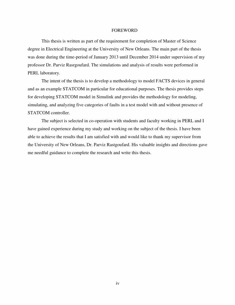
FOREWORD

This thesis is written as part of the requirement for completion of Master of Science

degree in Electrical Engineering at the University of New Orleans. The main part of the thesis

was done during the time-period of January 2013 until December 2014 under supervision of my

professor Dr. Parviz Rasrgoufard. The simulations and analysis of results were performed in

PERL laboratory.

The intent of the thesis is to develop a methodology to model FACTS devices in general

and as an example STATCOM in particular for educational purposes. The thesis provides steps

for developing STATCOM model in Simulink and provides the methodology for modeling,

simulating, and analyzing five categories of faults in a test model with and without presence of

STATCOM controller.

The subject is selected in co-operation with students and faculty working in PERL and I

have gained experience during my study and working on the subject of the thesis. I have been

able to achieve the results that I am satisfied with and would like to thank my supervisor from

the University of New Orleans, Dr. Parviz Rastgoufard. His valuable insights and directions gave

me needful guidance to complete the research and write this thesis.

v

TABLE OF CONTENTS

Table of Contents.....................................................................................................v

List of Figures ....................................................................................................... vii

List of Tables .......................................................................................................... x

Abstract .................................................................................................................. xi

Chapter 1..................................................................................................................1

Introduction..............................................................................................................1

1.1 Introduction to FACTS Devices ........................................................................2

1.2 Types of Fault ....................................................................................................3

1.2.1 Balanced Three-Phase Fault Analysis ............................................................4

1.2.2 Unbalanced Fault Analysis .............................................................................4

1.3 Review of Relevant Studies ...............................................................................6

1.4 Objective of the Thesis ......................................................................................7

Chapter 2 Model of the Power System ....................................................................8

Chapter 3 Model of the Power System with STATCOM .....................................22

3.1 STATCOM Overview......................................................................................22

3.2 STATCOM Operating Principle ......................................................................23

3.3 Modeling of STATCOM in Simulink..............................................................24

Chapter 4 Test System ...........................................................................................31

4.1 Balanced Three-Phase Fault ............................................................................31

4.2 Three Phase-to-Ground Fault...........................................................................37

4.3 Line-to-Ground Fault .......................................................................................42

4.4 Line-to-Line Fault ............................................................................................47

4.5 Double Line-to-Ground Fault ..........................................................................52

Chapter 5 Results and Analysis .............................................................................57

5.1 Balanced Three-Phase Fault ............................................................................58

5.2 Three Phase-to-Ground Fault...........................................................................61

5.3 Line-to-Ground Fault .......................................................................................62

5.4 Line-to-Line Fault ............................................................................................64

5.5 Double Line-to-Ground Fault ..........................................................................66

Chapter 6 Conclusion and Future Work ................................................................70

vi

References..............................................................................................................72

Appendix A............................................................................................................74

Appendix B ............................................................................................................75

Appendix C ............................................................................................................76

Appendix D............................................................................................................77

Appendix E ............................................................................................................78

Vita.........................................................................................................................79

vii

LIST OF FIGURES

Figure 1.1: Four Common Types of Fault ...............................................................4

Figure 1.2: (a) Balanced three phase fault, (b) Balanced three phase

to ground fault..........................................................................................................4

Figure 1.3: Line-to-ground fault on phase “c”.........................................................5

Figure 1.4: Line-to-Line Fault on phases “b-c” .......................................................5

Figure 1.5: Double Line-to-Ground Fault on phases “b-c” .....................................5

Figure 2.1: (a) One-line Diagram of the 4-bus System, (b) One-line Diagram of

the Test Power System with description in Table 2.1..............................................8

Figure 2.1c): Scheme of the Test System ................................................................9

Figure 2.2: AC Voltage Source Simulink Block ...................................................10

Figure 2.3: Load Representation in Simulink Block .............................................11

Figure 2.4: Three-phase Transformer Simulink Block ..........................................12

Figure 2.5: Distributed Transmission Line Simulink Block..................................16

Figure 2.6: Power System Model in Simulink.......................................................18

Figure 2.7 a): System Voltage Waveform Measured after Transformer ...............19

Figure 2.7 b): System Current Waveform Measured after Transformer ...............20

Figure 3.1: Static Compensator (STATCOM) System: Voltage Source Converter

(VSC) connected to the AC Network via a Shunt-Connected Transformer ..........22

Figure 3.2: Structure and Equivalent Circuit of STATCOM.................................23

Figure 3.3: Static Compensator (STATCOM) Equivalent Circuit ........................24

Figure 3.4: STATCOM Controller System............................................................24

Figure 3.5: A Thyristor in Parallel with a Series RC Circuit Subsystem ..............25

Figure 3.6: Voltage Source Inverter Model ...........................................................26

Figure 3.7: One-line Diagram of the Power System with STATCOM

Controller ...............................................................................................................26

Figure 3.8: Model of the Power System with STATCOM in Simulink ................27

Figure 3.9 a): System Voltage Waveforms Measured after Transformer..............28

Figure 3.9 b): System Current Waveforms Measured after Transformer ..............29

Figure 4.1: One-line diagram of the balanced three-phase fault............................32

Figure 4.2: Model without STATCOM under Balanced Three-Phase Fault .........33

viii

Figure 4.3: Model with STATCOM under Balanced Three-Phase Fault ..............34

Figure 4.4: Voltage plot of the power system without STATCOM

Under three-phase fault..........................................................................................35

Figure 4.5: Voltage plot of the power system with STATCOM

Under three-phase fault..........................................................................................36

Figure 4.6: One-line diagram of the three-phase to-ground fault ..........................37

Figure 4.7: Model without STATCOM under Three-Phase to Ground Fault........38

Figure 4.8: Model with STATCOM under Three-Phase to Ground Fault.............39


Under Three-Phase to Ground Fault ......................................................................40


Under Three-Phase to Ground Fault ......................................................................41

Figure 4.11: One-line Diagram of the Power System with Line-to-Ground

Fault .......................................................................................................................42

Figure 4.12: Model of the Power System without STATCOM

Under Line-to-Ground Fault ..................................................................................43

Figure 4.13: Model of the Power System with STATCOM






Figure 4.16: One-line Diagram of the Bus System with

Phase-to-Phase Fault (A-to-B)...............................................................................47

Figure 4.17: Model without STATCOM under Line-to-Line Fault ......................48

Figure 4.18: Model with STATCOM under Line-to-Line Fault............................49


Under Line-to-Line Fault .......................................................................................50


Under Line-to-Line Fault .......................................................................................51

Figure 4.21: One-line Diagram of the Power System with Double Line-to-Ground

ix

Fault .......................................................................................................................52

Figure 4.22: Model of the power system without STATCOM

Under Line-to-Ground fault...................................................................................53

Figure 4.23: Model of the power system with STATCOM






Figure 5.1 a): Voltage Peaks after the Balanced Three-Phase Fault Clears

In the System without STATCOM ........................................................................59

Figure 5.1 b): Voltage Peaks after the Balanced Three-Phase Fault Clears

In the System with STATCOM .............................................................................60

Figure 5.2 a): Voltage Peaks after the Three-Phase to Ground Fault Clears


Figure 5.2 b): Voltage Peaks after the Three-Phase to Ground Fault Clears


Figure 5.3 a): Voltage Peaks after the Line-to-Ground Fault Clears


Figure 5.3 b): Voltage Peaks after the Line-to-Ground Fault Clears


Figure 5.4 a): Voltage Peaks after the Line-to-Line Fault Clears


Figure 5.4 b): Voltage Peaks after the Line-to-Line Fault Clears


Figure 5.5 a): Voltage Peaks after the Double Line-to-Ground Fault Clears


Figure 5.5 b): Voltage Peaks after the Double Line-to-Ground Fault Clears


x

LIST OF TABLES

Table 2.1: Parameters of the Power System ..........................................................17

Table 3.1: Thyristor in Parallel with Series RC Circuit Simulink

Block Parameters ...................................................................................................25

Table 5.1: Comparison of Voltage Peaks for the System Without and

With STATCOM ...................................................................................................69

xi

ABSTRACT

The analysis of power systems under fault condition represents one of the most important

and complex tasks in power engineering. The study and detection of these faults are necessary to

ensure that the reliability and stability of the power system do not suffer a decrement as a result

of a critical event such as fault. The purpose of this thesis is to develop and to present an

educational tool for students to model FACTS devices using Simulink. Furthermore, the

development of this thesis provides the means for students to model different types of faults. The

development is based on presenting a power system – the Test System - by its simplest form

including generation, transmission, transformers, loads and STATCOM device as an example of

the general FACTS devices. The thesis includes modeling of the Test System using Simulink and

MATLAB program to produce the results for further analysis. The findings and development

included in the thesis is intended to serve as an educational tool for students interested in the

study of faults and their impact on FACTS devices. Students may use the thesis as the building

block for developing models of larger and more complex power systems using Simulink and

MATLAB programs for further study of impacts of FACTS devices in power systems.

Fault Analysis, Power Systems, Types of Fault, STATCOM, MATLAB, Modeling,

Simulink

1

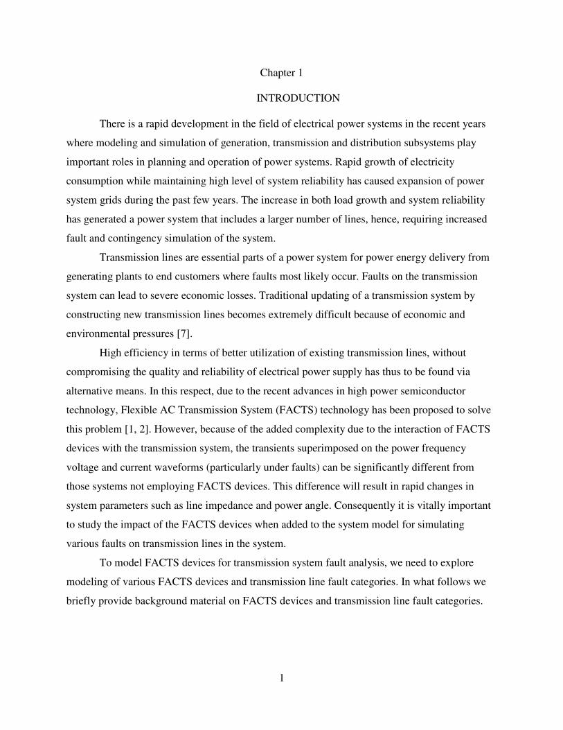
Chapter 1

INTRODUCTION

There is a rapid development in the field of electrical power systems in the recent years

where modeling and simulation of generation, transmission and distribution subsystems play

important roles in planning and operation of power systems. Rapid growth of electricity

consumption while maintaining high level of system reliability has caused expansion of power

system grids during the past few years. The increase in both load growth and system reliability

has generated a power system that includes a larger number of lines, hence, requiring increased

fault and contingency simulation of the system.

Transmission lines are essential parts of a power system for power energy delivery from

generating plants to end customers where faults most likely occur. Faults on the transmission

system can lead to severe economic losses. Traditional updating of a transmission system by

constructing new transmission lines becomes extremely difficult because of economic and

environmental pressures [7].

High efficiency in terms of better utilization of existing transmission lines, without

compromising the quality and reliability of electrical power supply has thus to be found via

alternative means. In this respect, due to the recent advances in high power semiconductor

technology, Flexible AC Transmission System (FACTS) technology has been proposed to solve

this problem [1, 2]. However, because of the added complexity due to the interaction of FACTS

devices with the transmission system, the transients superimposed on the power frequency

voltage and current waveforms (particularly under faults) can be significantly different from

those systems not employing FACTS devices. This difference will result in rapid changes in

system parameters such as line impedance and power angle. Consequently it is vitally important

to study the impact of the FACTS devices when added to the system model for simulating

various faults on transmission lines in the system.

To model FACTS devices for transmission system fault analysis, we need to explore

modeling of various FACTS devices and transmission line fault categories. In what follows we

briefly provide background material on FACTS devices and transmission line fault categories.

2

1.1. Introduction to FACTS Devices

The Thyristor Controlled Series Capacitor (TCSC), the Universal Power Flow Controller

(UPFC), the Static Synchronous Series Compensator (SSSC), and the Static Synchronous

Compensator (STATCOM) are some of the power controllers developed under the umbrella

name of “Flexible AC Transmission Systems” (FACTS). These devices play a key role in

modern electrical networks because they have the capability of improving the operation and

control of power networks by increasing power transfer and improving transient stability among

other characteristics. Collateral to their many strong points, the FACTS controllers have

undesired impact on the protection system that should be taken into account in modeling,

simulation, and design of future power systems.

The FACTS controllers, once installed in the power grid, help to improve the power

transfer capability of long transmission lines and the system performance in general.

Additionally FACTS controllers are beneficially used for fast voltage regulation, increased

power transfer over long AC lines, damping of active power oscillations, and load flow control

in meshed systems.

Hingorani and Gyugyi [3] provide a useful and thorough representation of FACTS

devices in four categories that are used by researchers in study and design of power systems. The

four categories represented in [3] and used in this thesis are:

1. Series Controller. Series controllers are connected to a power line in series and have an

impact on the power flow and voltage profile. Examples of these controllers are the SSSC and

TCSC.

2. Shunt Controllers. These controllers are shunt connected to transmission lines and are

designed to inject current into the system at the point of connection. An example of these

controllers is the Static Synchronous Compensator (STATCOM).

3. Series-shunt controllers. These controllers are a combination of serial and shunt

controllers. This combination is capable of injecting current and voltage. An example of

controllers is the Unified Power Flow Controller (UPFC).

4. Series-series controllers. These controllers can be a combination of separate series

controllers in a multiline transmission system, or it can be a single controller in a single line. An

example of such devices is the Interline Power Flow Controller (IPFC). The STATCOM, TCSC,

3

and SSCC are three of the FACTS controllers highlighted by their capacity to provide a wide

range of solutions for both normal and abnormal conditions.

The TCSC is made of a series capacitor (CTCSC) shunted by a thyristor module in series

with an inductor (LTCSC). An external fixed capacitor (CFIXED) provides additional series

compensating. Normally the TCSC operates as a variable capacitor, firing the thyristor between

180° to 150°.

The SSSC injects a voltage in series with the transmission line in quadrature with the line

current. The SSSC increases or decreases the voltage across the line, and thereby, controlling the

transmitted power.

The STATCOM is a voltage-source converter (VSC) based controller which maintains

the bus voltage by injecting an ac current through a transformer.

The STATCOM can rapidly supply dynamic VARs required during system faults for

voltage support. During a fault in power system short circuit currents flow, the magnitude of

these currents can be of the order of tens of thousands of amperes. So consequently, the fault

types have to be determined and analyzed.

With this brief background material on FACTS devices, we proceed to providing the

necessary material on types of faults that are important building blocks in our study of faulted

power systems that include FACTS devices [10].

1.2 Types of Faults

Granger and Stevenson [8] outlined balanced three-phase faults, single line-to-ground

faults, line-to-line faults, double line-to-ground faults as four common types of fault occurrence

on transmission lines. Figure 1.1 provides a graphical view of the four types of faults.

4

Figure 1.1: Four Common Types of Fault [8]

1.2.1 Balanced Three-Phase Fault

Balanced three-phase fault is defined as the simultaneous short circuit across all three

phases of a transmission line. A three phase fault is a condition where either (a) all three phases

of the system are short circuited to each other or (b) all three phases of the system are grounded.

Figure 1.2 provides a pictorial view of balanced three-phase faults.

Figure 1.2: (a) Balanced three phase fault, (b) Balanced three phase to ground fault [8]

Balanced three phase fault is also called as symmetric fault because the power system

remains in balance after the fault occurs. It is the most infrequent but the most severe fault type,

and other faults, if not cleared promptly, can easily develop into a three-phase fault [8].

1.2.2 Unbalanced Faults

Single line-to-ground faults are faults in which an overhead transmission line touches the

ground because of wind, ice loading, or a falling tree limb. A majority of transmission line faults

are single line-to-ground faults. The single line to ground fault can occur in any of the three

5

phases. However, it is sufficient to analyze only one of the phases [8]. Figure 1.3 depicts line-to-

ground fault on phase “c”.

Figure 1.3: Line-to-ground fault on phase “c” [8]

Line-to-line faults are usually the result of galloping lines because of high winds or

because of a line breaking and falling on a line below. Line-to- line faults may occur in a power

system, with or without the earth, and with or without fault impedance [8]. Figure 1.4 shows

line-to-line fault on phases “b-c”.

Figure 1.4: Line-to-line fault on phases “b-c” [8]

Double line-to-ground fault occurs when two phases got shorted to the ground. This type

of fault is common due to the storm damage. Double line-to-ground fault is presented on Figure

1.5.

Figure 1.5: Double line-to-ground fault on phases “b-c” [8]

So far we have provided problem statement, FACTS devices and four common categories

that are used by researchers in their studies, and four common types of faults experienced on

6

transmission lines. We next provide a summary of the studies that have been conducted and

reported by investigators using FACTS devices.

1.3 Review of Relevant Studies

Varieties of fault studies and some research have been done on the performance of

distance relays for transmission systems including different FACTS devices and are reported in

literature. The analytical results based on steady-state model of STATCOM, and the impact of

STATCOM on distance relays at different load levels are presented in [18]. In [19], the voltage-

source model of FACTS devices is used to study the impact of FACTS on tripping boundaries of

distance relays.

The work in [20] shows that thyristor controlled series capacitor (TCSC) has a big

influence on the mho characteristic and reactance while the studies in [21], [15] and [4]

demonstrate that the presence of FACTS devices on a transmission line will affect the trip

boundary of distance relays, and both the parameters of the FACTS device and its location have

impacts on the trip boundary.

Wavelet transform based multi resolution analysis approach can be successfully applied

for effective detection and classification of faults in transmission lines. With STATCOM

controller, fault detection, classification and location can be accomplished within a half cycle

using detail coefficients of currents [13, 16]. Wavelet transform is an effective tool in

analyzing transient voltage and current signals associated with faults both in frequency

and time domain.

The new wavelet-fuzzy combined approach for digital relaying is highly used nowadays

as well. The algorithm for fault classification employs wavelet multi resolution analysis (MRA)

to overcome the difficulties associated with conventional voltage and current based

measurements due to effect of factors such as fault inception angle, fault impedance and fault

distance. The combined approach employs wavelet transform together with fuzzy logic. The

wavelet transform captures the dynamic characteristics of the non-stationary

transient fault signals using wavelet MRA coefficients. The fuzzy logic is employed to

incorporate expert evaluation through fuzzy inference system (FIS) so as to extract

important features from wavelet MRA coefficients for obtaining coherent conclusions

regarding fault location [16].

7

All the studies show that when the FACTS device is in a fault loop, its voltage and

current injection will affect both the steady and transient components in voltage and current and

hence the apparent impedance seen by a conventional distance relay is different from that on a

system without FACTS.

When the types of faults described in Section 1.2 occur, the magnitude of bus voltage

cannot exist at its operational range, either voltage drops or increases. To prevent this effect,

STATCOM FACTS controller is the best solution to maintain bus voltage magnitude in a

suitable range [1]. There is always a need to develop innovative methods for transmission line

protection.

1.4 Objectives of the Thesis

The first objective of this thesis is to study in dynamics the common fault types that occur

in the power system. Secondly is to perform the analysis of influence that FACTS devices and in

particular STATCOM has on a power system under five categories of faults described in Section

1.2. These objectives are accomplished by creating a model of a power system in Simulink –

MATLAB based program. Simulink is the environment in MATLAB that has design tools to

model and simulate a power system. Simulink has been used to build the STATCOM [2,5,6,9]

and to study different types of influences that it has on a power system described in Section 1.3.

We focus on studying the influence of STATCOM on a test power system during fault

event. Moreover, we simulate, analyze, and compare the results of five different types of faults

on the test system without and with STATCOM model.

The remainder of the thesis is organized to include the necessary parts in order to

determine the effect of the STATCOM on a power system. So firstly the model of a power

system is developed in Chapter 2. Secondly STATCOM controller was introduced into the

system and analyzed in Chapter 3. In Chapter 4 five different types of faults were added in the

power system with STATCOM. Chapter 5 includes the analysis of STATCOM influence on the

power system and concluding remarks and future work are included in Chapter 6.

8

Chapter 2

MODEL OF THE POWER SYSTEM

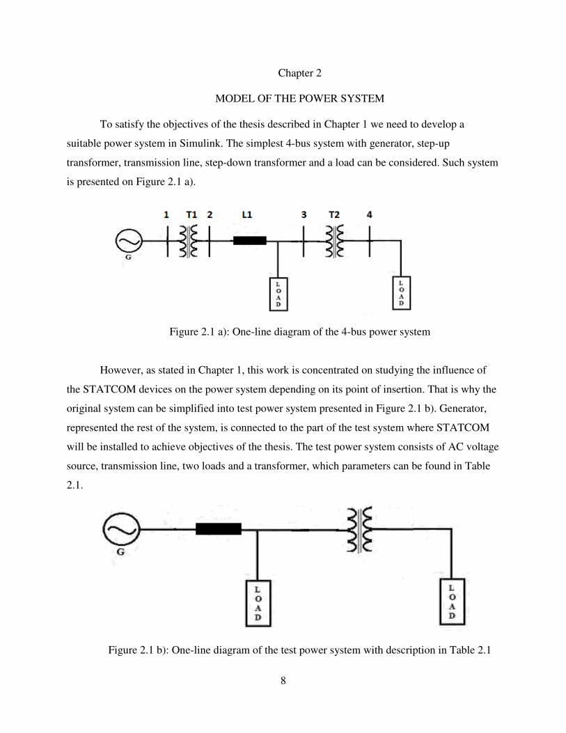
To satisfy the objectives of the thesis described in Chapter 1 we need to develop a

suitable power system in Simulink. The simplest 4-bus system with generator, step-up

transformer, transmission line, step-down transformer and a load can be considered. Such system

is presented on Figure 2.1 a).

Figure 2.1 a): One-line diagram of the 4-bus power system

However, as stated in Chapter 1, this work is concentrated on studying the influence of

the STATCOM devices on the power system depending on its point of insertion. That is why the

original system can be simplified into test power system presented in Figure 2.1 b). Generator,

represented the rest of the system, is connected to the part of the test system where STATCOM

will be installed to achieve objectives of the thesis. The test power system consists of AC voltage

source, transmission line, two loads and a transformer, which parameters can be found in Table

2.1.

Figure 2.1 b): One-line diagram of the test power system with description in Table 2.1

9

The test power system can be presented as a scheme consisting of a part where

STATCOM will be installed and the rest of the system. Depending on the point of STATCOM

insertion, test system can be modified for the future studies. Scheme of a power system used in

this work is presented in Figure 2.1 c).

Figure 2.1 c): Scheme of the test system

The generator in the test system is modeled by a voltage source and for analysis of the

results, the generator is an ideal voltage source in Simulink. Although in real power systems

generators’ characteristics are not ideal, the choice of power source was to simplify the analysis

using Simulink results. The AC voltage source used to model the generator of Figure 2.1 b) is

represented by Figure 2.2.

AC voltage source model in Simulink was presented by three-phase ideal sinusoidal

voltage source with amplitude of 3

2735000 ⋅ volts and with three phases lagging each other by

120 degrees.

10

Figure 2.2: AC voltage source Simulink block

The two loads in Figure 2.1 b) are represented as inductive instead of resistive loads. It is

important to have inductive and not just resistive loads in order to achieve the similarity with a

real world power system. Two loads were added into two different places of the power system:

one on the generation side and one after step-down transformer on the load side. Simulink

models of the load are shown by Figure 2.3.

11

Figure 2.3: Load representation in Simulink block

Transformer is also added into the system to achieve the similarity with the real world

power system. It is a step-down transformer from generation side of the model to the load side.

Three-phase transformer block of the Simulink power system model is presented in Figure 2.4.

Three-phase transformer model in Simulink was built by specifying parameters for

winding 1 and winding 2, and also magnetization characteristics which are the following:

Winding 1 parameters: [V1 Ph-Ph(Vrms), R1(pu), L1(pu)]= [735e3, 0.15/30/2, 0.15*0.7]

Winding 2 parameters: [V2 Ph-Ph(Vrms), R2(pu), L2(pu)]= [ 16e3, 0.15/30/2, 0.15*0.3]

Magnetization resistance: [Rm (pu); magnetization inductance Lm (pu)]= [500, 500]

12

Figure 2.4: Three-phase transformer Simulink block

In order to simulate transmission line, distributed model of the line with specific R, L and

C values that are shown in Table 2.1 were chosen. Transmission line is the model block that has

to be explained in more details since its values change depending on the length of the line. Thus,

we will present the necessary theory for distributed parameter model of transmission lines in this

section. A distributed parameter is a parameter which is spread throughout a structure and is not

confined to a lumped element such as a coil of wire.

The generic line consists of two conductors with a potential difference V(x) between

them, and a current I(x) that flows down one conductor, and returns via the other. A current

flowing in a wire gives rise to a magnetic field, H. By the definition L, the inductance of a circuit

element, L≡ΦI, is Φ, the flux linking the circuit element, multiplied by I, the current flowing

through it. But the longer a section of wire is, the more Φ would be needed for the same I.

Thus, L as the distributed inductance for the transmission line has to be defined. It has units of

Henrys per unit length and can be found as length of transmission line multiplied by a distributed

inductance of L. The two conductors would also have a distributed capacitance C which has units

of Farads per unit length and can be found as the length of transmission line multiplied by

distributed capacitance C. Thus, we see that the transmission line has both a distributed

inductance L and a distributed capacitance C which are tied up with each other. There is really no

13

way in which we can separate one from the other having only the capacitance, or only the

inductance; there will always be some of each associated with each section of line no matter how

small or how big we make it [12].

These elements of transmission line such as capacitance and reactance may be used in the

per phase equivalent circuit of a three-phase line operating under balanced conditions. The

Distributed Parameter Line block, used in Simulink, implements an N-phase distributed

parameter line model with lumped losses. The model is based on the Bergeron's traveling wave

method [5]. In this model, the lossless distributed LC line is characterized by two values (for a

single-phase line): the surge impedance c

lZC = and the wave propagation speed

clv

⋅

=1

,

where l and c are the per-unit length inductance and capacitance [12]. For the test model used in

the simulations, distributed parameters of the transmission line such as resistance presented by

resistance per unit length (Ohms/km) specified by positive and zero-sequence resistances [r1 r0]-

[0.01273 0.3864]. Inductance presented by inductance per unit length (H/km) with positive and

zero-sequence inductances [l1 l0]- [0.9337e-3 4.1264e-3]. Capacitance presented by

capacitance per unit length (F/km) specified by positive and zero-sequence capacitances [c1 c0]-

[12.74e-9 7.751e-9]. Positive, negative and zero-sequence components are used to resolve

unbalanced three-phase systems into balanced system of phasors. The symmetrical components

differ in the phase sequence, that is, the order in which the phase quantities go through a

maximum. The phase components are the addition of the symmetrical components and can be

written as follows:

021

021

021

cccc

bbbb

aaaa

++=

++=

++=

(2.1)

In order to solve the system (2.1) it has to be written in terms of one phase, for example

phase “a”, components and the operatorα , which has a magnitude of unity and, when operated

on any complex number, rotates it anti-clockwise by an angle of 120 degrees. The operatorα ,

the square of it and (1+j0) phasor form a balanced symmetrical system [12].

If Za, Zb, and Zc are the impedance of the load between phases “a”, “b”, and “c”, then

sequence impedances are given in (2.2):

14

)(3

1:

)(3

1:

)(3

1:

3

2

1

cba

cba

cba

ZZZZzero

ZZZZnegative

ZZZZpositive

++=

++=

++=

α

α

(2.2)

Transmission lines are assumed to have positive and negative sequence to be equal [12],

so only positive sequence was mentioned in the test system. Taking into account the numbers

from the test model for inductance specified by positive and zero-sequence inductances [l1 l0]-

[0.9337e-3 4.1264e-3] and capacitance specified by positive and zero-sequence capacitances

[c1 c0]- [12.74e-9 7.751e-9], we can get the following equations specified in (2.3):

9751.7)(3

1

974.12)(3

1

974.12)(3

1

31264.4)(3

1

3933.0)(3

1

3933.0)(3

1

0

0

−=++=

−=++=

−=++=

−=++=

−=++=

−=++=

ecccc

ecccc

ecccc

ellll

ellll

ellll

cba

cbaneg

cbapos

cba

cbaneg

cbapos

α

α

α

α

(2.3)

Solving the above system of equations (2.3) in Matlab program the following solutions

were found:

)0432.00748.0()0071(

)0432.00748.0()0071(

)0864.03822.0()0071(

0028.00048.0

0028.00048.0

0055.00028.0

jec

jec

jec

jl

jl

jl

c

b

a

c

b

a

−−⋅−=

−−⋅−=

+⋅−=

−=

−=

−=

(2.4)

Transmission lines may be represented by a single reactance in the single line diagram as

l and c are the per-unit length inductance and capacitance. For a lossless line (r = 0), the

quantity e + Zci, where e is the line voltage at one end and i is the line current entering the same

end, must arrive unchanged at the other end after a transport delay τ.

v

d=τ (2.5)

where d is the line length and v is the propagation speed [12]. Using the notion of propagation

speed and surge impedance, the following can be established in (2.6):

15

c

lZC = (2.6)

cld ⋅=τ

The model equations for a lossless line are:

)()()()( ττ −⋅+−=⋅− tiZtetiZte Scsrcr (2.7)

)()()()( ττ −⋅+−=⋅− tiZtetiZte rcrScS

knowing that,

)()(

)( tIZ

teti sh

SS −= (2.8)

)()(

)( tIZ

teti rh

rr −=

In a lossless line, Ish and Irh, which are two current sources of a two-port model, are computed in

(2.9):

)()(2

)( ττ −−−⋅= tIteZ

tI rhr

c

sh (2.9)

)()(2

)( ττ −−−⋅= tIteZ

tI shS

c

rh

When losses are taken into account, new equations for Ish and Irh (2.10) are obtained by

lumping R/4 at both ends of the line and R/2 in the middle of the line:

R = total resistance = r × d

The current sources Ish and Irh are then computed as follows [12]:

))()(1

()2

1())()(

1()

2

1()( ττττ −⋅−−⋅

+⋅

−+−⋅−−⋅

+⋅

+= tIhte

Z

hhtIhte

Z

hhtI shSrhrsh (2.10)

))()(1

()2

1())()(

1()

2

1()( ττττ −⋅−−⋅

+⋅

−+−⋅−−⋅

+⋅

+= tIhte

Z

hhtIhte

Z

hhtI rhrshSrh

where

4

rZZ C +=

4

4r

Z

rZ

h

C

C

+

−

= (2.11)

16

For multiphase line models, modal transformation is used to convert line quantities from

phase values (line currents and voltages) into modal values independent of each other. As the test

model is three-phase unbalanced system, it would have to be solved by taking the values of

phase components separately and converting them into modal quantities. This can be

accomplished by using transformations like Karrenbauer, Clarke or alike which are commonly

used in EMPT-like programs. These transformations result in the same modal impedances and

admittances as would result from applying symmetrical components transformation in the 60 Hz

phase domain [5]. These transformations are automatically performed inside the Distributed

Parameter Line block of Simulink which model is presented on Figure 2.5.

Figure 2.5: Distributed transmission line Simulink block

Numerical values for each of the components of the power system are described next.

The system consists of 600 km transmission line powered by 735 kV generator. A 735kV/16kV

Delta/Y transformer connected to the power system to step down the voltage. Two loads 330 and

17

250 MW each are installed on the power system as well. The details of the power system are

presented in the Table 2.1.

Table 2.1: Parameters of the power system

Generator 735kV 3 phase AC voltage source

Load 1 330MW/250 Active, 330MVar Reactive

Load 2 250MW/250 Active, 250MVar Reactive

Transmission line Length=600km, R= 0.01273 Ohm/km,

L= 0.9337e-3 H/km, C= 12.74e-9 F/km

Putting all the components together into one model, we receive graphical representation

of the power system built in Simulink which is shown in Figure 2.6.

After simulations had been performed the voltage and current can be observed at the

various locations of the system. This is done by including the graph blocks for plotting voltage

and current waveforms (Figure 2.7).

18

Ideal Voltage

Source

Continuous

powergui

v+-

Voltage Measurement

U3 no statcom

U2

U1

Transmission Line

(600 km)

A B C

a b c

Three-phase Transformer

735/16kV

Vabc

Iabc

A B C

a b c

Three-Phase

V-I Measurement1

Vabc

Iabc

A B C

a b c

Three-Phase

V-I Measurement

I2

I1

C1B1A1

A B C

330 MVar

Load

A B C

250 MVar

Load

Figure 2.6: Power system model in Simulink

19

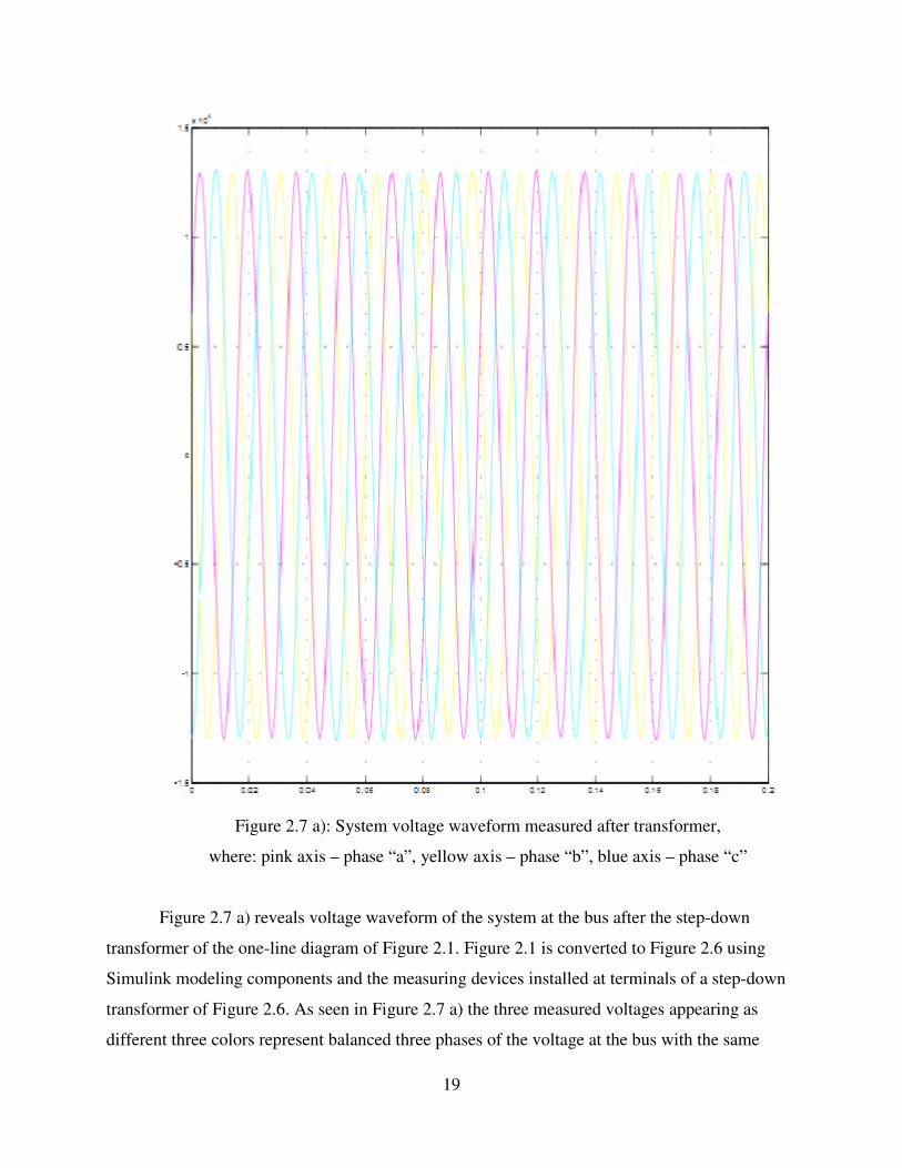
Figure 2.7 a): System voltage waveform measured after transformer,

where: pink axis – phase “a”, yellow axis – phase “b”, blue axis – phase “c”

Figure 2.7 a) reveals voltage waveform of the system at the bus after the step-down

transformer of the one-line diagram of Figure 2.1. Figure 2.1 is converted to Figure 2.6 using

Simulink modeling components and the measuring devices installed at terminals of a step-down

transformer of Figure 2.6. As seen in Figure 2.7 a) the three measured voltages appearing as

different three colors represent balanced three phases of the voltage at the bus with the same

20

magnitude and 120 degrees phase angle. Figure 2.7 b) is a replica of 2.7 a) except for the current

phases at the bus.

Figure 2.7 b): System current waveform measured after transformer,


In Chapter 3 we introduce model of STATCOM in the Simulink model of Chapter 2 for

running “what if scenarios” while applying different faults. The developed integrated Simulink

model could be used for studying behavior of STATCOM when the transmission system is

21

exposed to faults in Chapter 4. The purpose of the developments of Chapter 3 and Chapter 4 is to

provide the educational tool for studying behavior of power systems that are pushed to their

stability limit and to study the improvements made by adding FACTS control devices in general

and STATCOM in particular. As stated in [14], STATCOM allows an increase in transfer of

power while improving stability limits by adjusting the power system parameters such as

voltage, current, frequency and phase angle.

22

Chapter 3

MODEL OF THE TEST POWER SYSTEM INCLUDING STATCOM

3.1 STATCOM Overview

A static synchronous compensator (STATCOM), also known as a "static synchronous

condenser" ("STATCON"), is a regulating device used on alternating current electricity

transmission networks [1]. STATCOM is a self commutated switching power converter supplied

from an electric energy source and operated to produce a set of adjustable multiphase voltage,

which may be coupled to an AC power system for the purpose of exchanging independently

controllable real and reactive power. The controlled reactive compensation in electric power

system is usually achieved with the variant STATCOM configurations. The STATCOM has

been defined with following three operating structural components. First component is Static:

based on solid state switching devices with no rotating components; second component is

Synchronous: analogous to an ideal synchronous machine with three sinusoidal phase voltages at

fundamental frequency and the third component is Compensator: provided with reactive

compensation. It is based on a power electronics voltage-source converter and can act as either a

source or sink of reactive ac power to an electricity network. If connected to a source of power it

can also provide active ac power. It is a member of the FACTS family of devices [3], [17].

Figure 3.1: Static compensator (STATCOM) system: voltage source converter (VSC)

connected to the AC power system via a shunt-connected transformer [3]

Usefully a STATCOM is installed to support electricity networks that have a poor power

factor and often poor voltage regulation and the most common use of it is for voltage stability. A

static synchronous compensator is a voltage source converter based device where the voltage

source is created from a DC capacitor and therefore a static synchronous compensator has very

23

little active power capability. However, STATCOM active power capability can be increased if a

suitable energy storage device is connected across the dc capacitor. The reactive power at the

terminals of the static synchronous compensator depends on the amplitude of the voltage source.

For example, if the terminal voltage of the voltage source converter (VSC) is higher than the ac

voltage at the point of connection, the STATCOM generates reactive current and when the

amplitude of the voltage source is lower than the ac voltage, it absorbs reactive power. The

response time of a STATCOM is shorter than that of a static var compensator (SVC), mainly due

to the fast switching times provided by the Insulated Gate Bypolar Transistor (IGBTs) of the

voltage source converter. The STATCOM also provides better reactive power support at low ac

voltages than an SVC, since the reactive power from a STATCOM decreases linearly with the ac

voltage (as the current can be maintained at the rated value even down to low ac voltage) [10].

3.2 STATCOM Operating Principle

A STATCOM consists of a coupling transformer, an inverter and a DC capacitor as

shown in Figure 3.2.

Figure 3.2: Structure and equivalent circuit of STATCOM [3]

STATCOM is usually used to control transmission voltage by reactive power shunt

compensation. Based on the operating principle of the STATCOM [3] the equivalent circuit has

been derived, which is displayed by Figure 3.3.

24

Figure 3.3: Static compensator (STATCOM) equivalent circuit [3]

In the derivation, it is assumed that the harmonics generated by the STATCOM are

neglected and the system as well as the STATCOM is three phases balanced. The STATCOM is

equivalently represented by a controllable fundamental frequency positive sequence shunt

voltage source. In principle of the STATCOM output voltage can be regulated in such a way that

the reactive power of the STATCOM can be changed [11].

3.3 Modeling of STATCOM in Simulink

In order to study improvement of transfer capability and voltage control of the power

system 6-pulse STATCOM was installed on the low side of the transformer of Figure 2.1 c). The

control model of STATCOM that is used in the test system is shown in Figure 3.4.

Inverter 1

Out1

3 C2 B1 A

imp_1

imp_4

Uab x

X

Thyristor

block 3

imp_1

imp_4

Uab x

X

Thyristor

block 2imp_1

imp_4

Uab x

X

Thyristor

block 1

U_lin

alfa

imp U Y

U Y

U Y

signalrms

RMS

KP2KP1KP

Ikr

Ia_rms

i+

-

DI4

i+

-

DI2

i+

-

DI1

u+90

Bias

2

alfa

1

Ulin

Figure 3.4: STATCOM controller system

25

The STATCOM consists of six IGBT inverters and three phase-shifting transformers.

Each inverter uses a thyristor in parallel with a series RC circuit block to generate almost square-

wave voltage. The parameters of the STATCOM control system are presented in Table 3.1.

Table 3.1: Thyristor in parallel with a series RC circuit Simulink block parameters

Resistance Ron 0.001 Ohm

Inductance Lon 1.13e-3 H

Snubber resistance Rs 500 Ohm

Snubber capacitance Cs 250e-9 F

The parameters represent the Simulink internal resistance Ron and internal inductance

Lon of the thyristor model as well as snubber parameters – resistance Rs and capacitance Cs. The

parameters are true when thyristor is in the on-state, and hence, “on” for representing internal

resistance and inductance.

This model is represented on Figure 3.5.

2 x

1 X

u,i,imp_4

u,i,imp_1

gm

ak

VT2

gm

ak

VT1

3 Uab 2 imp_41 imp_1

Figure 3.5: A thyristor in parallel with a series RC circuit subsystem

26

The inverters of Figure 3.4 with specifications of Figure 3.5 are fed to the secondary

windings (L=18.7e-3 H) of phase-shifting transformers whose primary windings are connected to

produce an almost sinusoidal voltage output.

The voltage source inverter in this research is represented with the help of a synchronized

6-pulse generator which can be viewed in the Figure 3.6.

1

impStep2 Prod

alpha_deg

A

B

C

Block

pulses

6-Pulse1

2

alfa

1 U_lin

Figure 3.6: Voltage source inverter model

The subsystems of Figure 3.4, 3.5, and 3.6 complete the STATCOM model which is used

to inject or decrease reactive power to regulate the voltage to the test system. The STATCOM

model is added to the low side of the transformer that is connected to the rest of the system at its

high side voltage bus. The “rest of the system” is represented by a generator, a load, a

transformer, and a transmission line with specific numerical values for simulation purposes. The

one-line diagram of “the rest of the system” connected to the load and the STATCOM model is

shown by Figure 3.7.

Figure 3.7: One-line diagram of the power system with STATCOM controller

The model of the power system with the STATCOM controller in Simulink is shown in

Figure 3.8.

27

Ideal Voltage Source


735/16kV

Continuous

powergui

v+-

Voltage Measurement

U3

U2

U1

Transmission Line

(600 km)

A B C

a b c

Vabc

Iabc

A B C

a b c

Three-Phase

V-I Measurement1

Vabc

Iabc

A B C

a b cThree-Phase

V-I Measurement

AB,BC,CA_Y

A B C

Subsystem4

Ulin

alfa

Out1 A B C

STATCOM

Itir

I2

I1

31

Constant

C1B1A1

A B C

330 MVar

Load

A B C

250 MVar

Load

Figure 3.8: Model of the power system with STATCOM controller in Simulink

28

Figure 3.9 shows voltage and current waveforms after performing simulations that

include model of the STATCOM. The waveforms will later be compared with the waveforms of

Chapter 2 which excludes STATCOM model.

Figure 3.9 a): System voltage waveforms measured after transformer

29

Figure 3.9 b): System current waveforms measured after transformer


We can see from the current graph of Figure 3.9 b) that the STATCOM injected about

20% current into the system which is necessary for increasing transfer capability and improving

voltage control. In voltage stability and control problems voltage decreases due to insufficient

power delivered to the loads. In order to prevent system from collapsing, it is necessary to inject

the additional reactive power into the system. This is especially crucial for the transmission lines,

since they are generally long and transfer of reactive power over these lines is very difficult due

30

to significant amount of reactive power requirement. STATCOM, by injecting reactive power

into the system, helps to prevent or lessen the problems of transfer capability of the system.

STATCOM can be also a solution for voltage control problems. Voltage control can be attained

by sufficient generation and transmission of energy. The main reason for voltage instability is the

lack of sufficient reactive power in the system, which can be regulated by STATCOM by

injecting current into the system which can be observably seen on Figure 3.9 b).

The performance of the power system is affected by many factors and particularly faults

on transmission lines. The Simulink model and simulations of the test system including

STATCOM and fault models provide the means to students for studying effectiveness of using

FACTS devices in general and STATCOM controller as an example. Chapter 4 includes steps

for modeling and simulation of five different types of fault and STATCOM controller for

analysis of the Test System of Chapter 3.

31

Chapter 4

TEST SYSTEM

To validate the ability of STATCOM to stabilize voltage in power system using Simulink

as an educational tool, the most common types of faults described in the Chapter 1 are simulated

in Chapter 4 using different scenarios and models. Specifically, we model and simulate five

types of faults:

- balanced three-phase fault;

- three-phase fault to the ground;

- line-to-ground fault;

- line-to-line fault;

- double line-to-ground.

Development of the educational methodology consists of two steps: a specific type of

fault is modeled and integrated in the model of the test system without STATCOM model while

recording the results of simulation; and inclusion of the model of STATCOM controller in the

test system while simulating different types of faults. The developed educational tool may then

be used for simulating “what if scenarios” by applying different fault types at different locations

in the test system with further modeling and inclusion of other FACTS devices than STATCOM.

The simulations were performed for 2 seconds consisting of 120 cycles to better observe

three time periods that are present in the simulations: time before the fault, time during the fault

and time after the fault. Time period after the fault can be divided into two sub-periods: time

immediately after the fault and the time during which the system goes into steady state. Results

from both experiments are summarized in Table 4.1.

4.1 Balanced three-phase fault

One-line diagram of the balanced three-phase fault is presented on the Figure 4.1.

32

Figure 4.1: One-line diagram of the balanced three-phase fault

Figure 4.2 represents the model of the power system without STATCOM under balanced

three-phase fault in Simulink. Whereas Figure 4.3 represents the model of the power system with

STATCOM under balanced three-phase fault in Simulink.

The parameters of the three-phase breaker are shown in Appendix A.

33



735/16kV

Continuous

powergui

v+-

Voltage Measurement

U3 no statcom

U2

U1

Transmission Line 1

(300 km)1

Transmission Line 1

(300 km)

A B C

a b c

A B C

a b c

Three-Phase Breaker

Vabc

Iabc

A B C

a b c

Three-Phase

V-I Measurement1

Vabc

Iabc

A B C

a b c

Three-Phase

V-I Measurement

I2

I1

C1B1A1

A B C

330 MVar

Load

A B C

250 MVar

Load

Fig 4.2: Model without STATCOM under balanced three-phase fault

34



735/16kV

250MVar

Load

Continuous

powergui

v+-

Voltage Measurement

U3

U2 with ST

U1

Transmission Line 1

(300 km)

Transmissio Line 1

(300 km)1

A B C

a b c

A B C

a b c

Three-Phase Breaker

Vabc

Iabc

A B C

a b c

Three-Phase

V-I Measurement1

Vabc

Iabc

A B C

a b c

Three-Phase

V-I Measurement

AB,BC,CA_Y

A B C

Subsystem4

Ulin

alfa

Out1 A B C

STATCOM

Itir

I2

I1

31

Constant

C1B1A1

A B C

330 MVar

Load

A B C

Fig 4.3: Model with STATCOM under balanced three-phase fault

The voltage graph of the power system without STATCOM under three-phase fault is

shown on Figure 4.4.

35

Fig 4.4: Voltage plot of the power system without STATCOM under three-phase fault

The voltage graph of the power system with STATCOM under three-phase fault is shown

on Figure 4.5.

36

Figure 4.5: Voltage plot of the power system with STATCOM under three-phase fault

Comparing the Figures 4.4 and 4.5, we can conclude that peak voltages of the system

with STATCOM are smaller than the system without one. The more detailed analysis of the

results will be presented in Chapter 5.

37

4.2 Three-phase-to-ground fault

One-line diagram of the three-phase to ground fault is presented on the Figure 4.6.

Figure 4.6: One-line diagram of the three-phase to ground fault

Figure 4.7 represents the model of the power system without STATCOM under three-

phase to ground fault in Simulink. Whereas Figure 4.8 represents the model of the power system

with STATCOM under three-phase to ground fault in Simulink.

The parameters of the three-phase breaker are shown in Appendix A.

38


Three-phase to ground Breaker


735/16kV

Continuous

powergui

v+-

Voltage Measurement

U3 no statcom

U2

U1

Transmission Line 1

(300 km)1

Transmission Line 1

(300 km)

A B C

a b c

A

B

C

a

b

c

Vabc

Iabc

A B C

a b c

Three-Phase

V-I Measurement1

Vabc

Iabc

A B C

a b c

Three-Phase

V-I Measurement

I2

I1

C1B1A1

A B C

330 MVar

Load

A B C

250 MVar

Load

Figure 4.7: Model without STATCOM under three-phase to ground fault

39


Three-phase to ground Breaker


735/16 kV

Continuous

powergui

v+-

Voltage Measurement

U3

U2

U1

Transmission Line 1

(300 km)1

Transmission Line 1

(300 km)

A B C

a b c

A

B

C

a

b

c

Vabc

Iabc

A B C

a b c

Three-Phase

V-I Measurement1

Vabc

Iabc

A B C

a b c

Three-Phase

V-I Measurement

AB,BC,CA_Y

A B C

Subsystem4

Ulin

alfa

Out1 A B C

STATCOM

Itir

I2

I1

31

Constant

C1B1A1

A B C

330 MVar

Load

A B C250 MVar

Load

Figure 4.8: Model with STATCOM under three-phase to ground fault

The voltage graph of the power system without STATCOM under three-phase to ground

fault is shown on Figure 4.9.

40

Figure 4.9: Voltage plot of the power system without STATCOM under three-phase to

ground fault

The voltage graph of the power system with STATCOM under three-phase to ground


41

Figure 4.10: Voltage plot of the power system with STATCOM under three-phase to

ground fault

42

Analyzing Figure 4.9 and 4.10 and the numerical values from the Table 5.1 in Chapter 5,

we can make the conclusion that installation of the STATCOM in the system with three-phase to

ground fault was the most effective. More detailed results are presented in Chapter 5.

4.3 Line-to-ground fault

One-line diagram of the line-to-ground fault is presented on the figure 4.11.

Figure 4.11: One-line diagram of the power system with line-to-ground fault

The model of the power system without STATCOM under line-to-ground fault in

Simulink is presented in the Figure 4.12. Whereas Figure 4.13 represents the model of the power

system with STATCOM under line-to-ground fault in Simulink.

The parameters of the line-to-ground breaker are shown in Appendix B.

43


Line-to-ground Breaker


735/16kV

250 MVar

Load

Continuous

powergui

v+-

Voltage Measurement

U3 no statcom

U2 no statcom

U1

Transmission Line 1

(300 km)1

Transmission Line 1

(300 km)

A B C

a b c

A

B

C

a

b

c

Vabc

Iabc

A B C

a b c

Three-Phase

V-I Measurement1

Vabc

Iabc

A B C

a b c

Three-Phase

V-I Measurement

I2

I1

C1B1A1

A B C

330 MVar

Load

A B C

Figure 4.12: Model of the power system without STATCOM under line-to-ground fault

44


Line-to-ground Breaker


735/16kV

Continuous

powergui

v+-

Voltage Measurement

U3

U2 with ST

U1 with ST

Transmission Line 1

(300 km)1

Transmission Line 1

(300 km)

A B C

a b c

A

B

C

a

b

c

Vabc

Iabc

A B C

a b c

Three-Phase

V-I Measurement1

Vabc

Iabc

A B C

a b c

Three-Phase

V-I Measurement

AB,BC,CA_Y

A B C

Subsystem4

Ulin

alfa

Out1 A B C

STATCOM

Itir

I2

I1

31

Constant

C1B1A1

A B C

330 MVar

Load

A B C250 MVar

Load

Figure 4.13: Model with STATCOM under line-to-ground fault

The voltage graph of the power system without STATCOM under line-to-ground fault is


45

Figure 4.14: Voltage plot of the power system without STATCOM under line-to-ground

fault

The voltage graph of the power system with STATCOM under line-to-ground fault is


46

Figure 4.15: Voltage plot of the power system with STATCOM under line-to-ground

fault

Numerical values of the voltage peaks from the Table 5.1, which concludes the results

from Figures 4.14 and 4.15, indicate that installation of the STATCOM into the system with line-

to-ground fault was effective as the voltage peaks are smaller when STATCOM is in the system.

47

4.4 Line-to-line fault

One-line diagram of the line-to-line fault is represented on the figure 4.16.

Figure 4.16: One-line diagram of the bus system with phase-to-phase fault (A-to-B)

Line-to-line fault can occur between any two phases. However, it is sufficient to analyze

only one case between two phases. In this work A-to-B fault was analyzed. Figure 4.17

represents the model of the power system without STATCOM under line-to-line fault in

Simulink. Whereas Figure 4.18 represents the model of the power system with STATCOM under

line-to-line fault in Simulink.

The parameters of the line-to-line breaker are shown in Appendix C.

48



735/16 kV

Continuous

powergui

v+-

Voltage Measurement

U3

U2

U1

Transmission Line 1

(300 km)1

Transmission Line 1

(300 km)

A B C

a b c

Vabc

Iabc

A B C

a b c

Three-Phase

V-I Measurement1

Vabc

Iabc

A B C

a b c

Three-Phase

V-I Measurement

Line-to-line Breaker

I2

I1

C1B1A1

A B C

330 MVar

Load

A B C

250 MVar

Load

Figure 4.17: Model without STATCOM under line-to-line fault

49



735/16 kV

Continuous

powergui

v+-

Voltage Measurement

U3

U2 with ST

U1

Transmission Line 1

(300 km)1

Transmission Line 1

(300 km)

A B C

a b c

Vabc

Iabc

A B C

a b c

Three-Phase

V-I Measurement1

Vabc

Iabc

A B C

a b c

Three-Phase

V-I Measurement

AB,BC,CA_Y

A B C

Subsystem4

Ulin

alfa

Out1 A B C

STATCOM

Line-to-line Breaker

Itir

I2

I1

31

Constant

C1B1A1

A B C

330 MVar

Load

A B C

250 MVar

Load

Figure 4.18: Model with STATCOM under line-to-line fault

The voltage graph of the power system without STATCOM under line-to-line fault is


50

Figure 4.19: Voltage plot of the power system without STATCOM under line-to-line

fault

The voltage graph of the power system with STATCOM under line-to-line fault is shown

on Figure 4.20.

51

Figure 4.20: Voltage plot of the power system with STATCOM under line-to-line fault

Placing STATCOM into the system with line-to-line fault was the second most effective

after three-phase to ground fault as the results in Table 5.1 indicate. The voltage peaks were

much smaller in the system with STATCOM than in the one without it.

52

4.5 Double line-to-ground fault

One-line diagram of the model with double line-to-ground fault is presented on figure

4.21.

Figure 4.21: One-line diagram of the power system with double line-to-ground fault

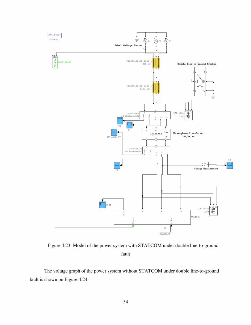
Figure 4.22 represents the model of the power system without STATCOM under double

line-to-ground fault in Simulink. Whereas Figure 4.23 represents the model of the power system

with STATCOM under double line-to-ground fault in Simulink.

The parameters of the double line-to-ground breaker are presented in Appendix D.

53


Double Line-to-ground Breaker


735/16 kV

Continuous

powergui

v+-

Voltage Measurement

U3 no statcom

U2

U1

Transmission Line 1

(300 km)1

Transmission Line 1

(300 km)

A B C

a b c

A

B

C

a

b

c

Vabc

Iabc

A B C

a b c

Three-Phase

V-I Measurement1

Vabc

Iabc

A B C

a b c

Three-Phase

V-I Measurement

I2

I1

C1B1A1

A B C

330 MVar

Load

A B C

250 MVar

Figure 4.22: Model of the power system without STATCOM under double line-to-ground

fault

54


Double line-to-ground Breaker


735/16 kV

Continuous

powergui

v+-

Voltage Measurement

U3

U2 with ST

U1

Transmission Line 1

(300 km)1

Transmission Line 1

(300 km)

A B C

a b c

A

B

C

a

b

c

Vabc

Iabc

A B C

a b c

Three-Phase

V-I Measurement1

Vabc

Iabc

A B C

a b c

Three-Phase

V-I Measurement

AB,BC,CA_Y

A B C

Subsystem4

Ulin

alfa

Out1 A B C

STATCOM

Itir

I2

I1

31

Constant

C1B1A1

A B C

330 MVar

Load

A B C

250 MVar

Load

Figure 4.23: Model of the power system with STATCOM under double line-to-ground

fault

The voltage graph of the power system without STATCOM under double line-to-ground


55

Figure 4.24: Voltage plot of the power system without STATCOM under double line-to-

ground fault

The voltage graph of the power system with STATCOM under double line-to-ground


56

Figure 4.25: Voltage plot of the power system with STATCOM under double line-to-

ground fault

The result presented in Figure 4.25 completes the modeling and simulation of five

categories of faults applied to the test system with and without model of STATCOM. We

analyze the results recorded in Chapter 4 in Chapter 5.

57

Chapter 5

RESULTS AND ANALYSIS

Using the models of STATCOM, the test system connecting the load bus with

STATCOM injection, and the rest of the system and the models of five categories of faults in

Simulink; the students may simulate different types of fault for studying the impact of

STATCOM on steady state and dynamic performance of the test system. All documented

studies of Chapter 4 show that when model of STATCOM is included in the loop, its voltage and

current injection will affect both the steady and transient response of voltage and current, and

hence their values will be different from those on a system without STATCOM model. In what

follows, we present a brief analysis of the responses comparing the impact of STATCOM model

using Simulink for educational purposes. To compare the effect of inclusion of STATCOM in

modeling the test system, we will use the index of Equation 5.1 for Peak Voltage improvement.

I1 = [1- (Peak Voltage without STATCOM )/(Peak Voltage with STATCOM)] (5.1)

The purpose of Chapter 5 is to simulate the models developed in Chapter 4 and to

compare the load bus voltage profile with and without inclusion of STATCOM for interested

students. To simulate a larger test system, the steps appearing in Chapter 4 and the simulation

outcomes of Chapter 5 may be used by students as building blocks of modeling and simulating

larger systems. The educational tool presented in the thesis may be followed by students for

modeling other FACTS devices than STATCOM. Furthermore, for analysis purpose and for

determining the usefulness of FACTS devices in a power system, students may use other metrics

than the index of Equation 5.1. We present other sample indices by Equation 5.2 and Equation

5.3.

I2 = [1 – (Oscillation without STATCOM)/(Oscillations with STATCOM)] (5.2)

In Equation 5.2, we count the number of oscillations before reaching steady state voltage

value with and without inclusion of STATCOM model in the test system. Use of STATCOM

may result in a stable voltage profile with lesser number of oscillations – appoint that may be

58

investigated by students using the educational modeling tool development of using Simulink in

Chapter 4.

As a third index, we may use the settling time to steady state value of voltage with and

without inclusion of STATCOM in the test system. Equation 5.3 provides the settling time index.

I3 = [1-(Settling time without STATCOM)/(Settling time with STATCOM)] (5.3)

In Equation 3, the settling time is measured between the start of the fault time and up to

the time of reaching steady state after the fault is removed and the system has reached its steady

state operation. While the proposed measures in Equation 5.2 and Equation 5.3 are not intended

for use in this thesis, they may be used by students for analyzing power systems that include

FACTS devices and the developments of the thesis in future.

5.1 Balanced three-phase fault

Let us model balanced three – phase fault with and without model of STATCOM in the

Simulink test system. Students may use modeling of the components of the system including

fault model of Chapter 4 to study the impact of inclusion of STATCOM controller in load bus

voltage and current performance before, during, and after the specific simulated fault is cleared.

Figure 5.1 and Figure 5.2 depict the performance of the test system at the load bus measured by

observing the voltage profile of the bus in the three time periods.

59

Figure 5.1 a): Voltage peaks after the balanced three-phase fault clears in the system

without STATCOM

60

Figure 5.1 b): Voltage peaks after the balanced three-phase fault clears in the system with

STATCOM

The three colors in Figure 5.1 and Figure 5.2 represent the three voltage phases on the

vertical axis versus time on the horizontal axis. The peaks of the voltage after the fault clears are

almost the same in the system with or without STATCOM. Using the index of Equation 5.1,

students may compare the impact of STATCOM in three periods of time. It seems that

STATCOM has minimal or no impact on Peak Voltage during or after the balanced three-phase

61

fault is cleared. The numerical value of peak voltage is included in the summary Table 5.1.

Table 5.1 may be expanded to include indices proposed by Equation 5.1, 5.2, and 5.3.

5.2 Three-phase to ground fault

For the power system under three-phase to ground fault STATCOM appeared to be the

most effective. The peak voltage of the system with STATCOM was lower than the one without

STATCOM. The steady-state value of the voltage was reached faster in the system with

STATCOM than in the one without it. The comparison of the voltage peaks is presented by

Figure 5.2. The numerical values are presented in the Table 5.1.

Figure 5.2 a): Voltage peaks after the three-phase to ground fault clears in the system

without STATCOM

62

Figure 5.2 b): Voltage peaks after the three-phase to ground fault clears in the system

with STATCOM

5.3 Line-to-ground fault

For the power system under line-to-ground fault STATCOM appeared to be effective.

The peak voltage of the system with STATCOM was lower than the one without STATCOM.

The steady-state value of the voltage was reached faster in the system with STATCOM than in

63

the one without it. The comparison of the voltage peaks is presented on figure 5.3. The numerical

values are presented in the Table 5.1.

Figure 5.3 a): Voltage peaks after the line-to-ground fault clears in the system without

STATCOM

64

Figure 5.3 b): Voltage peaks after the line-to-ground fault clears in the system with

STATCOM

5.4 Line-to-line fault

For the power system under line-to-line fault STATCOM appeared to be effective. The

peak voltage of the system with STATCOM was lower than the one without STATCOM. The

steady-state value of the voltage was reached faster in the system with STATCOM than in the

65

one without it. The comparison of the voltage peaks is presented on figure 5.4. The numerical

values are presented in the Table 5.1.

Figure 5.4 a): Voltage peaks after the line-to-line fault clears in the system without

STATCOM

66

Figure 5.4 b): Voltage peaks after the line-to-line fault clears in the system with

STATCOM

5.5 Double line-to-ground fault

For the power system under double line-to-ground fault STATCOM appeared to be

effective. The peak voltage of the system with STATCOM was lower than the one without

STATCOM. The steady-state value of the voltage was reached faster in the system with

67

STATCOM than in the one without it. The comparison of the voltage peaks is presented on

figure 5.5. The numerical values are presented in the Table 5.1.

Figure 5.5 a): Voltage peaks after the double line-to-ground fault clears in the system

without STATCOM

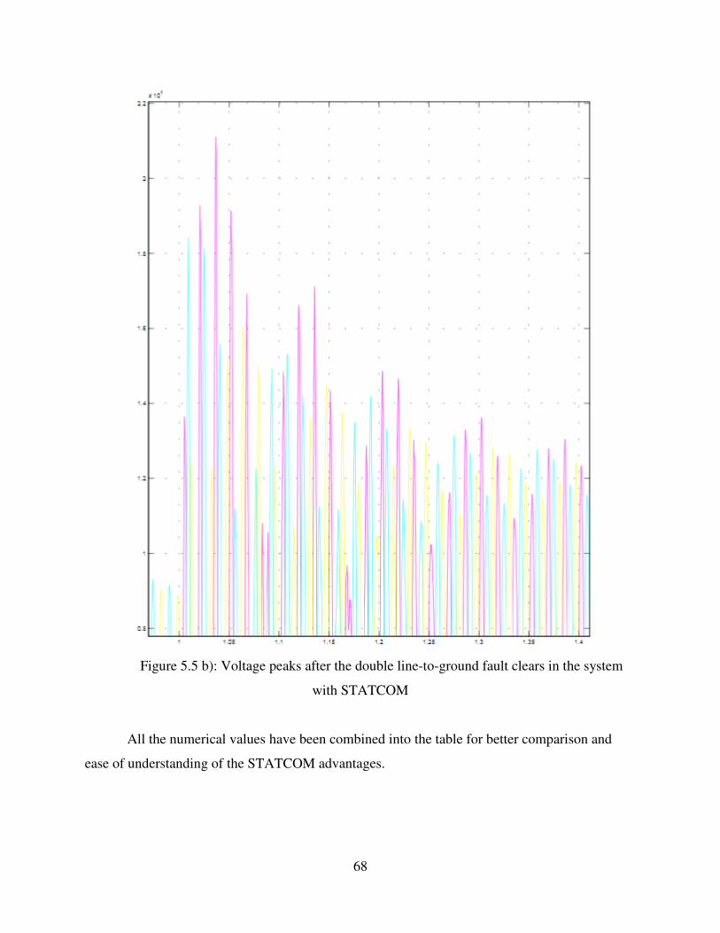
68

Figure 5.5 b): Voltage peaks after the double line-to-ground fault clears in the system

with STATCOM

All the numerical values have been combined into the table for better comparison and

ease of understanding of the STATCOM advantages.

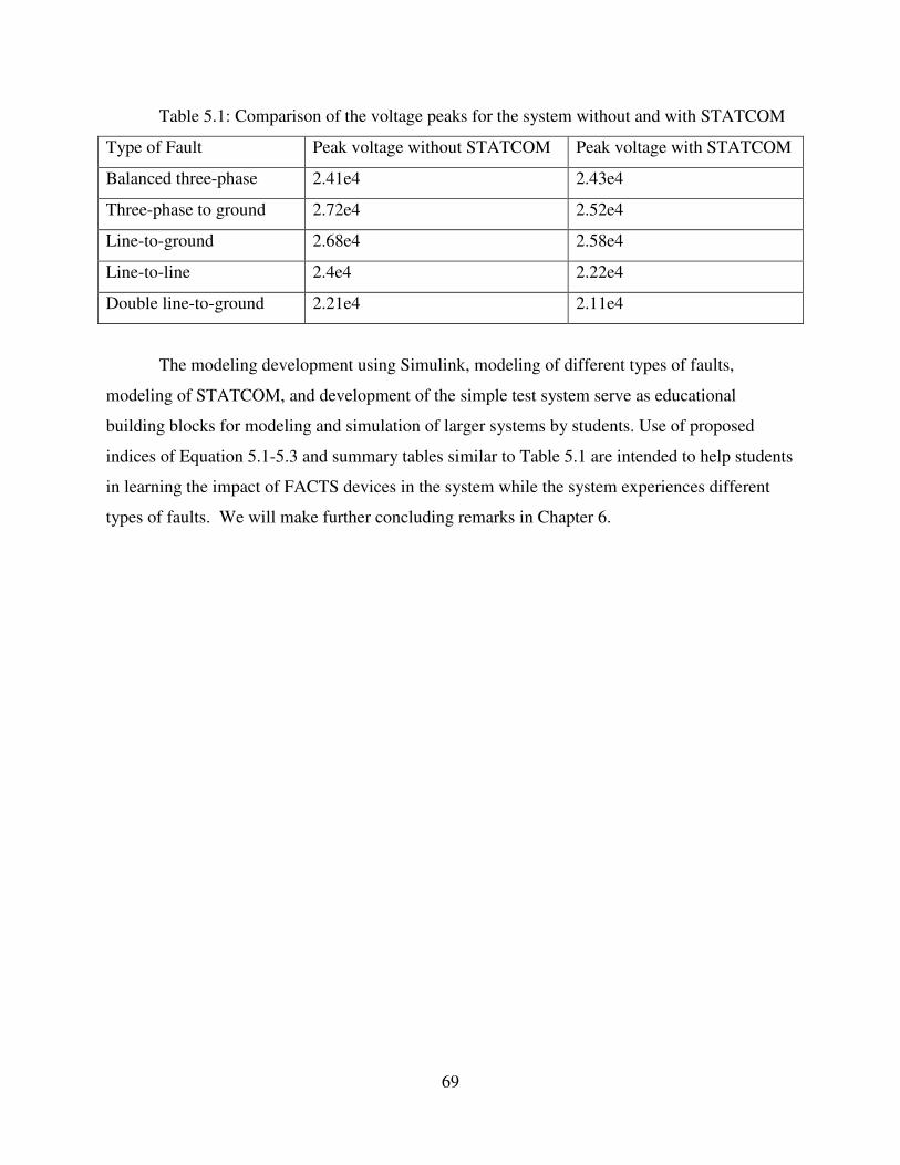
69

Table 5.1: Comparison of the voltage peaks for the system without and with STATCOM

Type of Fault Peak voltage without STATCOM Peak voltage with STATCOM

Balanced three-phase 2.41e4 2.43e4

Three-phase to ground 2.72e4 2.52e4

Line-to-ground 2.68e4 2.58e4

Line-to-line 2.4e4 2.22e4

Double line-to-ground 2.21e4 2.11e4

The modeling development using Simulink, modeling of different types of faults,

modeling of STATCOM, and development of the simple test system serve as educational

building blocks for modeling and simulation of larger systems by students. Use of proposed

indices of Equation 5.1-5.3 and summary tables similar to Table 5.1 are intended to help students

in learning the impact of FACTS devices in the system while the system experiences different

types of faults. We will make further concluding remarks in Chapter 6.

70

Chapter 6

CONCLUSIONS AND FUTURE WORK

STATCOM is one of the most widely used FACTS devices for efficient power system

operation. It is based on a voltage source converter and can inject or sink an almost sinusoidal

current with variable magnitude to an electricity network. If connected to a source of power it

can also provide active AC power. Usually a STATCOM is installed to support electricity

networks that have a poor power factor and often poor voltage regulation. There are however,

other uses, the most common use is for voltage stability.

It is widely used at the mid-point of a transmission line or heavy load area to maintain the

connecting point voltage by supplying or decreasing reactive power into the power system.

Because of the presence of STATCOM devices in a fault loop, the voltage and current signals

will be affected in both steady and transient state.

This thesis includes an educational methodology for modeling, simulating, and then

analyzing behavior of STATCOM when exposed to different types of faults. A power system is

first represented by and equivalent system connected to a load by two transformers and one

transmission line. The system is further reduced to a model where “the rest of the system” is

connected to a load bus by a transmission line where a STATCOM is connected to the high end

of the step-down transformer with a load. The proposed test system is therefore equipped with

the STATCOM model with appropriate sensing devices measuring three phase voltage and

current at the high and the low end of the step-down transformer.

The thesis includes classification and detail of fault types and a methodology for

modeling faults using Simulink. Using MATLAB, simulation studies of the Test-System that

includes models for faults and STATCOM were performed and measured by the voltage and

current sensors in three time periods; before, during, and post fault periods. To ensure capturing

the transient and steady state behaviors of the system including STATCOM and different fault

types, the voltage and current profiles at different locations in the system where observed and

recorded for 2 seconds – more than necessary time for the dynamics to settle at their steady state

values. The observed data is used in MATLAB to analyze the Test-System that includes

STATCOM and fault types.

71

After providing a methodology for modeling faults and STATCOM using Simulink, we

propose three indices in Chapter 5 that may provide educational insight to students for studying

usefulness of STATCOM in faulted power systems. Equations 5.1-5.3 and similar indices to

appear in future works at PERL (Power & Energy Research Laboratory) and other FACTS

devices than STATCOM will be pursued further. Studying Voltage Peak may be performed

using Equation 5.1 while frequency oscillation and settling time may be studied by use of

Equation 5.2 and 5.3.

This work describes the model of STATCOM in Simulink. MATLAB Simulink model

was used to simulate and analyze types of faults. In a very preliminary analysis and educational

purposes, the simulation results show the impact of STATCOM on the system. In particular

STATCOM device decreases voltage peaks and dips during and after a fault condition that

improves reaching stable state of the system with smaller overshoots.

This thesis may be extended to include larger number of buses by including a smaller in

size equivalent of the rest of the system, inclusion of faults at different locations than at the bus

where the STATCOM is connected to, inclusion of models of other FACTS devices than

STATCOM, and inclusion of generator and load dynamics in the larger test system. This thesis

provides the educational building blocks for students to study behavior of FACTS devices and

not as a tool for analysis of faulted power systems that include FACTS devices. The thesi

therefore may be used as building blocks for modeling and simulation of larger and more

realistic systems with the aid of Simulink and MATLAB. The proposed future works and

extensions will be performed by the student researchers in the University of New Orleans Power

and Energy research Laboratory.

72

REFERENCES

[1] Q. Yu, P. Li, and Wenhua, “Overview of STATCOM technologies,” in Proc. IEEE Int.

Conf. Electric Utility Deregulation, Restructing, PowerTechnologies, Hong Kong, Apr.

2004, pp. 647–652.

[2] P. Giroux, G. Sybille, and H. Le-Huy, “Modeling and simulation of a distribution

STATCOM using simulink’s power system blockset,” in Proc. Annu. Conf. IEEE

Industrial Electronics Society, pp. 990–994.

[3] N. G. Hingorani and L. Gyugyi, “Understanding FACTS, Concepts and Technology of

Flexible AC Transmission Systems”, Piscataway, NJ: IEEE Press, 2000.

[4] N. Vijaysimha, Ch.Chengaiah, “Evaluation of fault analysis in transmission lines using

relay settings”, Journal of Theoretical and Applied Information Technology, pp. 126-134.

[5] I.V.Chernyh, “Modeling of Electric Devices using MATLAB, SimPowerSystems and

Simulink”,DMK Press, 2008.

[6] J.Segunto-Ramirez and A.Medina, “Analysis of Power Electronic Controllers in Electric

Power Systems using Simulink”, Mexico, pp. 1-9.

[7] IEEE Power Engineering Society (PES), IEEE Guide for Determining Fault Location on

AC Transmission and Distribution Lines, IEEE Std. C37.114-2004.

[8] Granger, J. J. and W. D. Stevenson. “Power system analysis”, New York: McGraw-Hill,

1994

[9] S.K.Das, J.K.Moharana, “Design and Simulation of Small Signal Model of a STATCOM

for Reactive Power Compensation on Variation of DC link Voltage”, International Journal

of Engineering and Innovative Technology (IJEIT) Volume 2, Issue 5, November 2012

[10] Amit Garg and Sanjai Kumar Agarwal, “Voltage Control and Dynamic Performance of

Power Transmission System using STATCOM and its Comparison with SVC”,

International Journal of Advances in Engineering & Technology, Jan 2012.

[11] B. Singh, R. Saha, A. Chandra, K. Al-Haddad, “Static synchronous compensators

(STATCOM): a review”, IET Power Electron., Vol. 2, Issue. 4, pp. 297–324, 2009.

[12] Arthur R. Bergen, Vijay Vittal, “Power System Analysis”, Second Edition, Prentice Hall,

pp. 90-126, 2000

[13] R.Kameswara Rao , G.Ravi kumar , Shaik Abdul Gafoor ,S.S.Tulasi Ram, “Fault Analysis

of Double Line Transmission System with STATCOM Controller Using Neuro-Wavelet

Based Technique”, International Journal of Engineering and Technology Volume 2 No. 6,

June, 2012.

[14] Amit Debnath, Champa Nandi, “Voltage Profile Analysis during Fault with STATCOM”,

International Journal of Computer Applications (0975 – 8887) Volume 72– No.11, May

2013.

[15] X.Y Zhou, H.F Wang, R.K Aggarwal, P.Beaumont, “The Impact of STATCOM on

Distance Relay”, 15th PSCC, Liege, 22-26 August 2005.

73

[16] N. Zamanan, M. Gilany, “A Sensitive Wavelet-Based Algorithm for Fault Detection in

Power Distribution Networks”, ACEEE Int. J. on Communication, Vol. 02, No. 01, Mar

2011.

[17] Ashish Dewangan, Dr. Rn pate, “HVDC Transmission with STATCOM”, IOSR Journal of

Engineering May 2012, Vol. 2(5) pp: 1095-1101.

[18] K. El-Arroudi, G. Joos, D.T. McGillis, “Operation of the Impedance Protection Relay with

the STATCOM”, Power Delivery, IEEE Transaction on, Volume 17, Issue 2, April 2002

pp: 381-387.

[19] P.K. Dash., A.K. Pradhan, G. Panda, A.C. Liew, “Adaptive relay setting for flexible AC

transmission systems (FACTS) ,” Power Delivery, IEEE Transactions on , Volume 15,

Issue 1, Jan 2000 pp: 38 -43.

[20] W. G. Wang, X.G. Yin, J. Yu, X.ZH Duan, D.SH Chen, “The impact of TCSC on distance

protection relay,” Power System Technology, 1998. Proceedings. POWERCON '98. 1998

International Conference on, Volume 1, 18-21 Aug. 1998.

[21] M, Khederzadeh, “The impact of FACTS device on digital multifunctional protective

relays,” Transmission and Distribution Conference and Exhibition 2002: Asia Pacific.

IEEE/PES, Volume 3, 6-10 Oct. 2002 pp: 2043 – 2048.

74

APPENDIX A

Three-phase breaker block that is used in the model with balanced three-phase fault as

well as in the model with three-phase to ground fault has next parameters:

Figure A: Parameters of the three-phase breaker block in Simulink used for three-phase fault

75

APPENDIX B

Three-phase breaker block that is used in the model with line-to-ground fault (switching

only one phase – phase A – to ground) has next parameters:

Figure B: Parameters of the three-phase breaker block in Simulink used for line-to-ground fault

76

APPENDIX C

The ideal breaker block that is used in the model with line-to-line fault has next

parameters:

Figure C: Parameters of the ideal breaker block in Simulink used for line-to-line fault

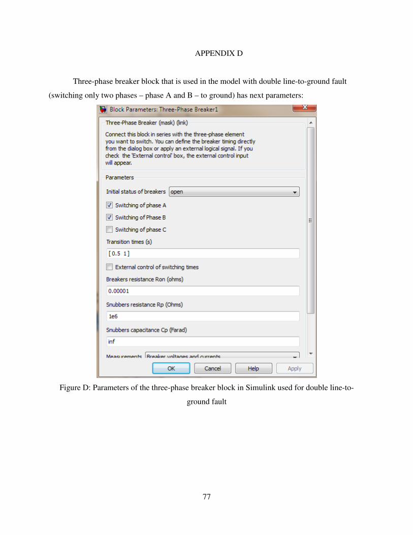
77

APPENDIX D

Three-phase breaker block that is used in the model with double line-to-ground fault

(switching only two phases – phase A and B – to ground) has next parameters:

Figure D: Parameters of the three-phase breaker block in Simulink used for double line-to-

ground fault

78

APPENDIX E

Transmission line in power system model in Simulink is represented by distributed

parameters line. It implements an N-phases distributed parameter line model. The R, L, and C

line parameters are specified by [NxN] matrices.

- Resistance presented by: resistance per unit length (Ohms/km) with [NxN matrix] -

[0.01273 0.3864].

- Inductance presented by: inductance per unit length (H/km) with [NxN matrix ] -

[0.9337e-3 4.1264e-3].

- Capacitance presented by: capacitance per unit length (F/km) with [NxN matrix] -

[12.74e-9 7.751e-9].

Three-phase transformer model in Simulink was built by specifying parameters for

winding 1 and winding 2, and also magnetization characteristics which are the following:

- Winding 1 parameters [V1 Ph-Ph(Vrms), R1(pu), L1(pu)]: [735e3, 0.15/30/2, 0.15*0.7].

- Winding 2 parameters [V2 Ph-Ph(Vrms), R2(pu), L2(pu)]: [ 16e3, 0.15/30/2, 0.15*0.3].

- Magnetization resistance Rm (pu): 500; magnetization inductance Lm (pu): 500.

AC voltage source model in Simulink was presented by three-phase ideal sinusoidal

voltage source with amplitude of 3

2735000 ⋅ with 120 degrees apart.

79

VITA

The author was born in Zaporizhzhya, Ukraine. She received Bachelor Degree in

Electrical Engineering from Zaporizhzhya National Technical University, Ukraine in 2008. She

obtained Master Degree in Electrical Engineering from Zaporizhzhya National Technical

University, Ukraine in 2009. She joined the University of New Orleans Electrical Engineering

graduate program in January 2012. She became a member of Dr. Parviz Rastgoufard research

team in January 2013. She is the member of IEEE professional organization since January 2013.

Documents

Educational Modeling for Fault Analysis of Power Systems