Education equity and intergenerational mobility: Quasi ... · education expenditure and parent income should lead to higher intergenerational mobility. Placing the magnitudes of these

Education equity and intergenerational mobility: Quasi-experimental evidence from court-

ordered school finance reforms

Minghao Li

Postdoctoral Research Associate

Iowa State University

Abstract

Starting from early seventies, court-ordered school finance reforms (SFRs) have

fundamentally changed the landscape of primary and elementary education finance in the US. This

paper employs SFRs as quasi-experiments to quantify the effects of education equity on

intergenerational mobility within commuting zones. First, I use reduced form difference-in-

difference analysis to show that 10 years of exposure to SFRs increases the average college

attendance rate by about 5.2% for children with the lowest parent income. The effect of exposure

to SFRs decreases with parent income and increases with the duration of exposure. Second, to

directly model the causal pathways, I construct a measure for education inequity based on the

association between school district education expenditure and median family income. Using

exposure to SFRs as the instrumental variable, 2SLS analysis suggests that one standard deviation

reduction in education inequality will cause the average college attendance rate to increase by 2.2%

for children at the lower end of the parent income spectrum. Placing the magnitudes of these effects

in context, I conclude that policies aimed at increasing education equity, such as SFRs, can

substantially benefit poor children but they alone are not enough to overcome the high degree of

existing inequalities.

Key words: public education finance, intergenerational mobility, school finance reforms, quasi-

experiments

I. Introduction

Starting from the Serrano v. Priest (1971) case in California, school finance lawsuits have

fundamentally changed the landscape of primary and secondary education finance in the United

States. In these lawsuits, the plaintiffs argued that the states had failed to provide just education

financing and demanded reforms. The courts that ruled in favor of reforms would order the state

legislatures to revise their education funding formulas. By channeling more state funds to poor

districts, these court-ordered school finance reforms (SFRs) have increased the equity of

education expenditures. A tally by Jackson, Johnson, and Persico (2015) counted that by 2010,

school finance lawsuits had been brought up in 42 states, some of which had experienced

multiple lawsuits (Figure 1). These lawsuits are still going on today and will continue to happen

in the future. Given their prevalence and importance, it is crucial to thoroughly evaluate the

effects of past SFRs.

This paper provides new evidence on the long-term impacts of SFRs on intergenerational

mobility, measured by the college attendance rates and child income rank. Exploiting SFRs as

natural experiments, this study also answers a broader question: To what degree, if any,

intergenerational mobility is causally determined by education equity?

The past literature on court-ordered SFRs agreed that they had achieved the fiscal goals

of curbing the within-state expenditure disparities (Murray, Evans, and Schwab 1998; Corcoran

and Evans 2008) and reducing the correlation between expenditure and family income (Card and

Payne 2002). Also, higher expenditure leads to more education inputs such as the number of

teachers per pupil and teacher salary (Jackson, Johnson, and Persico 2016). However, the effects

of SFRs on students’ outcomes during school are contested (Papke 2005; Guryan 2001; Downes

and Figlio 1998; Hoxby 2001; Fischel 2006; Hanushek 2003), and the evidence on the long-term

impacts of SFRs are very sparse. Card and Payne (2002) found tentative evidence that the

equalization caused by SFRs narrows the SAT score outcomes across parent education

categories. Jackson et al. (2016) found that the exogenous increase in school expenditures caused

by court-ordered SFRs raises low-income children’s income and education attainment. Besides

the lack evidence on the long-term impacts of SFRs in general, the effects of SFR on

intergenerational mobility have not been studied. Intergenerational mobility is defined over the

entire range of parent income, yet existing studies (such as Card and Payne 2002 and Jackson et

al. 2016) only grouped children by crude categories therefore cannot provide quantitative

predictions regarding intergenerational mobility.

[Insert Figure 1 here]

[Insert Figure 2 here]

Other than providing additional evidence for policy evaluation, quantifying the impacts

of SFRs on intergenerational mobility is also an important contribution to the mobility literature.

Previous theoretical studies reached no consensus on the effects of education equity on

intergenerational mobility: on one hand, more equitable education finance can transfer more

funds to poor students and increase mobility. On the other hand, over-centralized education

financing may weaken individual incentives to invest in education and decrease mobility (Solon

2004; Checchi, Ichino, and Rustichini 1999). The task of determining the relationship between

education equity and integrational mobility is left to empirical studies. While cross-country

studies provide suggestive correlational evidence, CHKS data offers a unique opportunity to

establish causal effects using panel data models. Although superior to cross-sectional analysis,

OLS analysis using panel data still suffers from serious endogeneity concerns. Public funding is

usually tied to the proportion of disadvantaged students, such as students who are learning

English as a second language. An increase in the proportion of these students would cause public

funding to increase. However, the positive impacts of additional funding might be offset by the

negative effects of unobservable student characters. SFRs generated exogenous changes in

education equity, which can be exploited as quasi-experiments to facilitate causal inference.

In this study, I use the differential trends of commuting-zone-level intergenerational

mobility across birth cohorts (Chetty, Hendren, Kline, and Saez 2014; Chetty et al. 2014, CHKS

from here on) to provide additional evidence on the long-term effects of SFRs. Using population

based federal tax records, CHKS provides college attendance rates (child income rank) for 10 (7)

birth cohorts from 1984 to 1993 (1980 to 1986), across the parent income distribution. Due to the

timing of SFRs, the duration of exposure to SFRs during school years varies from cohort to

cohort, which serves as the treatment variable that creates exogenous shifts in education equity.

The first part of the analysis uses the panel fixed effect model to evaluate the effects of

exposure to SFRs on children’s college attendance rates. The empirical setup is equivalent to the

difference-in-difference (DD) analysis in the panel data setting. I find that 10 years of exposure

to SFRs increases the average college attendance rate of lowest-parent-income children by

5.72%, and reduces the attendance gap between lowest and highest-parent-income children by

3.92%. Event analysis shows that the impact increases with the duration of exposure following

an approximately linear trend. Furthermore, as parent income rank increases, the impact of SFRs

diminishes, also in an approximately linear relationship. The impact of SFRs loses statistical

significance at about 70% parent income rank (100% being the highest). These results indicate

that, in the long-term, SFRs have substantial equalization effects on college attendance, and the

equalization is achieved by leveling-up, not leveling-down. However, similar analysis on child

income ranks finds now significant results. Possible reasons for not finding significant results for

income ranks are discussed.

The second part of the analysis quantifies the impacts of education expenditure equity on

intergenerational mobility, using exposure to SFRs as the instrumental variable. I first construct

education equity measures following Card and Payne (2002). For each cohort in each state, the

equity of education is measured by the expenditure-income gradient, defined as the association

(regression coefficient) between school district education expenditure per pupil and median

income. I find that exposure to SFRs reduces the expenditure-income gradient, and that one

standard deviation decrease in expenditure-income gradient increases the college attendance

rates for the lowest-parent-income students by 2.06% and reduces the college attendance

inequality by 2.87%. In contrast to the 2SLS results, OLS regressions produce unexpected

results, demonstrating the importance of addressing the endogeneity bias. Overall, these results

are consistent with the theoretical prediction (Solon 2004) that weakening the linkage between

education expenditure and parent income should lead to higher intergenerational mobility.

Placing the magnitudes of these effects in context, I concluded that policies aimed at increasing

education equity, such as SFRs, can substantially increase poor children’s college attendance but

they alone are not enough to overcome the high degree of existing inequalities.

The remainder of the paper is organized as follows. Section II outlines empirical

strategies and Section III introduces data. Section IV presents results from the DD analysis that

evaluates the impacts of SFRs on intergenerational mobility. Section V presents the 2SLS

estimations that quantifies the impacts of education equity on intergenerational mobility, using

exposure to SFRs as instruments, and Section VI concludes.

II. Empirical Strategy

II a. Difference-in-difference analysis of the impact of SFRs.

The objective of this part of the analysis is to test whether exposure to court-ordered

school finance reforms has positive impacts on various mobility measures, and if yes, quantify

the sizes of these impacts. For college attendance analysis (demonstrated in Figure. 3), the first

cohort in this study started school in 1990 and finished in 2002, while the last cohort started

school in 1999 and finished in 2011. For child income rank, the first cohort was born in 1980 and

the last cohort was born in 1986. The duration of exposure to SFRs during school years, ranging

from 0 to 12, is our key independent variable.

[Insert Figure 3 Here]

The mobility measures include the college attendance rates (income rank) of children

from various family backgrounds, measure by their parents’ income ranking. Another useful

measure of mobility is the slopes that characterize the linear relationships between the college

attendance rate (child income rank) and parent income ranking, which represent the outcome

gaps between children from highest and lowest income families. Let 𝑀𝑜𝑏𝑖𝑙𝑖𝑡𝑦𝑐𝑠𝑡 be the omnibus

symbol for the mobility measures for birth cohort 𝑡 in commuting zone 𝑐 of state 𝑠, the

regression model is of the following form:

𝑀𝑜𝑏𝑖𝑙𝑖𝑡𝑦𝑐𝑠𝑡 = 𝛽𝑒𝑥𝑝𝐸𝑥𝑝𝑜𝑠𝑢𝑟𝑒𝑠𝑡 + 𝛽𝑣𝑖𝑛𝑉𝑖𝑛𝑡𝑎𝑔𝑒𝑠𝑡 + 𝛽𝑐𝐶𝑜𝑣𝑎𝑟𝑖𝑎𝑡𝑒𝑠𝑐𝑠𝑡 + 𝜃𝑐 + 𝛾𝑡 + 𝜀𝑐𝑠𝑡 (1)

𝑉𝑖𝑛𝑡𝑎𝑔𝑒𝑠𝑡 = 𝑏𝑖𝑟𝑡ℎ_𝑦𝑟 + 6 − 𝑟𝑒𝑓𝑜𝑟𝑚_𝑦𝑟 𝑖𝑓 𝑏𝑖𝑟𝑡ℎ_𝑦𝑟 + 6 − 𝑟𝑒𝑓𝑜𝑟𝑚_𝑦𝑟 > 0, 0 𝑜𝑡ℎ𝑒𝑟𝑤𝑖𝑠𝑒

The coefficient 𝛽𝑒𝑥𝑝 is the main result of interest. For SFRs that happened before a certain cohort

entered school, the 𝑉𝑖𝑛𝑡𝑎𝑔𝑒𝑠𝑡 variable allows older reforms to have different impacts from more

recent reforms (Lafortune, Rothstein, and Schanzenbach 2016). I control for a host of commuting

zone-cohort level covariates to increase the precision of the model. Commuting zone fixed

effects are represented by 𝜃𝑐 which captures time-invariant omitted variables, cohort fixed

effects 𝛾𝑡 captures time variant omitted variables that are common to all commuting zones. With

the inclusion of both 𝜃𝑐 and 𝛾𝑡, this is the standard setup for a DD analysis in the panel data

setting with the treatments applied at different time points for different groups (in our case

states). In absence of the treatment (when 𝐸𝑥𝑝𝑜𝑠𝑢𝑟𝑒𝑠𝑡 is 0), this model assumes that commuting

zones will follow the same time trend 𝛾𝑡, which is the DD assumption. The error term 𝜀𝑐𝑠𝑡 is

clustered at the state level, allowing for within-state spatial correlations as well as

autocorrelations (Bertrand, Duflo, and Mullainathan 2004).

The above parametric model assumes the impact of SFRs to be proportional to the

duration of the exposure. However, non-linearity cn arise for various reasons. For instance, if

later investment in education depends on earlier investment, then SFRs will only have effects if

the duration of exposure is sufficiently long. On the other hand, if there are decreasing returns to

investment, then the effects of SFRs will plateau after certain amount of exposure. The following

semi-parametric specification is estimated to relax the linearity assumption:

𝑀𝑜𝑏𝑖𝑙𝑖𝑡𝑦𝑐𝑠𝑡 = ∑ 𝐸𝑥𝑝𝑜𝑠𝑢𝑟𝑒_𝑖𝑠𝑡

12

𝑖=−5

+ 𝛽𝑐𝐶𝑜𝑣𝑎𝑟𝑖𝑎𝑡𝑒𝑠𝑐𝑠𝑡 + 𝜃𝑐 + 𝛾𝑡 + 𝜀𝑐𝑠𝑡 (2)

In the above equation, the linear exposure variable in equation (1) is replaced by a set of dummy

variables 𝐸𝑥𝑝𝑜𝑠𝑢𝑟𝑒_𝑖𝑠𝑡, representing different exposure duration. For instance, 𝐸𝑥𝑝𝑜𝑠𝑢𝑟𝑒_8𝑠𝑡 =

1 if the cohort experienced exactly 8 years of SFRs, 𝐸𝑥𝑝𝑜𝑠𝑢𝑟𝑒_8𝑠𝑡 = 0 otherwise. Besides the

ability to capture non-linearity, this setup (sometime known as event analysis) can test for

preexisting trends. If court verdicts are truly exogenous, they should not have effects on cohorts

that missed the reform. On the other hand, if the observed treatment effect is the artifact of

certain unobserved trends, these trends will also have effects on cohorts that missed the

treatment. In this placebo test, we expect that dummy variables representing missing the SFRs

(i<0) to have little effects.

II b. 2SLS estimation of the impacts of education equity on intergenerational mobility

Intuitively, if public education financing becomes more equitable, children from poor

families are going to receive more resources resulting in higher levels of upward mobility. This

intuition is formalized in Solon’s (2004) model where the author shows that intergenerational

mobility, reversely measured by intergenerational elasticity, increases with the progressivity of

the public education system.

However, cross-country patterns of intergenerational mobility and education equity do

not always conform to this intuition and the predictions of Solon’s model. For example, Checchi

et al. (1999) present evidence that Italy, despite having a more egalitarian education system than

the U.S., exhibit less intergenerational mobility across occupations and education level. To

reconcile this paradox, the authors devised a theoretical model in which a centralized education

system could produce less intergenerational mobility compared to the private education system

by stifling individual efforts. Needless to say, causality cannot be established with a two-country

comparison. However, Checchi et al. (1999) demonstrate that the relationship between education

equity and intergenerational mobility is not theoretically given, and that more empirical evidence

is needed to establish the causality between the two.

One straightforward approach to estimate the impacts of education equity on

intergenerational mobility is to directly regress mobility measures on education equity measures

using the panel fixed effects model. Although superior to cross-sectional analysis, OLS analysis

using panel data still suffers from strong endogeneity concerns. Public funding is usually tied to

the proportion of disadvantaged students, such as students who are learning English as a second

language. An increase in the proportion of these students would cause public funding to increase.

However, the positive impacts of additional funding might be offset by the negative effects of

unobservable student characters.

In this part, I use court-ordered finance reform as the exogenous shifter to quantify the

causal impact of education equity on intergenerational mobility. Inequity measures are

constructed for each state-cohort pair using a method that is similar to that used in Card and

Payne (2002). The following school-district-level regression is estimated for each state 𝑠 and

cohort 𝑡:

𝑃𝑃𝐸𝑑 = 𝛽0, + 𝛽𝑖𝑛𝑐 ∗ 𝑚𝑒𝑑𝑖𝑎𝑛𝑖𝑛𝑐𝑑+ 𝛽𝑐𝑜𝑛𝐶𝑜𝑛𝑡𝑟𝑜𝑙𝑑 + 𝑒𝑑 (3)

School districts are index by 𝑑, the indexes for states and cohorts are suppressed. Total per pupil

expenditure 𝑃𝑃𝐸𝑑 is averaged over the period when the children is in school (from 6 to 18 years

old.) School district median family income 𝑚𝑒𝑑𝑖𝑎𝑛_𝑖𝑛𝑐𝑑 is measured at the time when the child

first enter school (6 years old). The coefficient of education expenditure regressed on median

family income 𝛽𝑖𝑛𝑐 is the measure of education inequality for that state/cohort (called

expenditure-income gradient, or EIG). Following Card and Payne (2002), the control variables

include dummy variables for school districts with less than 100 pupils, with 100 to 200 students,

and with 200 to 300 students; the log of the average school size within the district, the ratio of

population living in urban areas, and the ratio of black and native American population, all

measured when the cohort is 6-years-old. The regression is weighted by the number of pupils in

the school district.

State-cohort level education equity (reversely measured by EIG) is used as an

explanatory variable for the different measures of intergenerational mobility. It is assumed to be

endogenous to the determination of mobility, and is instrumented by the cohort’s exposure to

court-ordered SFRs using the 2SLS method:

𝐸𝐼𝐺𝑐𝑠𝑡 = 𝛽𝑟𝐸𝑥𝑝𝑜𝑠𝑢𝑟𝑒𝑠𝑡 + 𝛽𝑐1𝐶𝑜𝑣𝑎𝑟𝑖𝑎𝑡𝑒𝑠𝑐𝑠𝑡 + 𝜃𝑐 + 𝛾𝑡 + 𝜀𝑐𝑠𝑡 (4)

𝑀𝑜𝑏𝑖𝑙𝑖𝑡𝑦𝑐𝑠𝑡 = 𝛽𝑝𝐸𝐼�̂�𝑐𝑠𝑡 + 𝛽𝑐2𝐶𝑜𝑣𝑎𝑟𝑖𝑎𝑡𝑒𝑠𝑐𝑠𝑡 + 𝜃′𝑐 + 𝛾′𝑡 + 𝜀′𝑐𝑠𝑡 (5)

Because 𝐸𝐼�̂�𝑐𝑠𝑡 is an estimated coefficient, the first stage regression is weighted by the inverse of

the standard deviation of the equity estimation.

III. Data

III a. School Finance Lawsuits

Starting from the Serrano v. Priest 1971 case in California, school finance lawsuits had

been brought up in 42 states. Among them, 29 had at least one verdict in favor of reforms.

Political scientists and economist (Lynn 2011; Baicker and Gordon 2006) have found the results

of school finance lawsuits, often determined by intense and protracted legal battles, hard to

predict. Therefore, they are often considered as exogenous by economists.

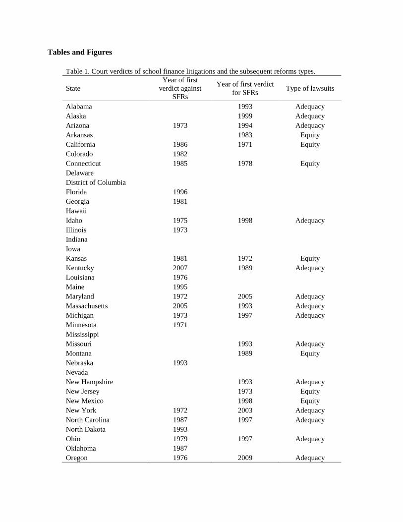
[Insert Table 1 Here]

Due to the broad interests in SFRs, inventories of school finance lawsuits have been

assembled by various sources. In this study, I adopt a recent catalog by Jackson et al. (2015),

which contains information for both legislative reforms and school finance lawsuits, the type of

the lawsuits, the results of the lawsuits, and the type of school finance formulas adopted before

and after the SFRs (table 1). In this study, I only consider the court-ordered reforms, because the

legislative reforms might be endogenous. Also, since a successful lawsuit may open the gate for

successive lawsuits, I only consider the first lawsuit overturning the existing system. Finally, the

treatment is defined by the result of the lawsuits, ignoring differences in the strength of state

response and the type of new funding formulas adopted. These responses are from the legislation

and are not exogenous to local conditions as court decisions. Therefore, the estimations in this

paper should be interpreted as the average total effect of initial SFRs and the subsequent SFRs

that they brought about.

III b. Mobility data

Intergenerational mobility data are published with the CHKS studies, and detail

information can be found in the original papers. Here I only provide a brief introduction to

facilitate readers’ understanding of the present study. Intergenerational mobility is measured at

the commuting-zone-level by the associations between children’s college attendance rate

(income rank) and their parents’ family income. These aggregates come from population based,

individual level federal tax records, which remain confidential to most researchers. The college

attendance (child income rank) data is available for 10 (7) birth cohorts from 1984 to 1993 (1980

to 1986).

College attendance is measured at age 19, child income is measured at age 26, and parent

income is measured when the children is 15 ~ 19 years old. Both child and parent income ranks

are national: for example, a parent income rank of 0.25 means that the parents’ family income is

higher than 25% of other parents of the child’s birth cohort in the US. Children are assigned to

locations based on where they were first claimed as dependents in tax records, regardless of

whether they migrated later on. Because the first year of the tax data is 1996, 98.9% of children

are assigned to their location in 1996 or 1997. CHKS showed that in a given geographical unit,

both the college attendance rate and child income rank have approximately linear relationships

with parent income rank and can be summarized by intercepts and slopes. The intercept

represents the average college attendance rate (income rank) of children with the lowest parent

income rank, while the slope represents the difference between children with the highest and the

lowest parent income rank. The average outcome of children with any parent income rank can be

calculated using the intercept and the slope. Because parent income is measured as national

ranks, the results are comparable across commuting zones.

III c. School districts finance and demographic data

State-cohort level education expenditure equity measures are constructed from school

district-level data. These data includes elementary and secondary school expenditure data from

Census of Government (compiled in Data Files on Historical Finances of Individual

Governments) and Local Education Agency Finance Survey (F-33) data from National Center

for Education Statistics (NCES). The former contains information for independent school

districts from 1967 to 2012, while the later contains all school districts from 1990 to 2010 (1991,

1993, and 1994 are not available). The NCES data is used when possible, and missing

observations are imputed using the average of the two nearby years. I only keep school districts

that have no missing data after imputation for all years under study (from 1990 to 2011). School

district characteristics are from Local Education Agency Universe Survey Data by NCES, which

contains enrollment and the number of schools. Demographic data for school districts include

median family income, the ratio of population living in urban areas, and the ratios of black and

Native American population, which can be found in the Census School District Tabulation Data

accessed through the School Districts Demographic System of NCES. For each cohort, the

expenditure variable is averaged over the years that the cohort is in primary and secondary

schools, and the school characteristics and demographic variables are measured at year when the

cohort is 6 years old. Demographic data are only available every 10 years, and the years in-

between are calculated using linear interpolations.

III d. Commuting-zone-level covariates

The following time-variant commuting zone level variables are included as controls to

increase the precision of the model. Medicaid benefits, Supplemental Nutrition Assistance

Programs (SNAP) benefits, and Earned Income Tax Credits (EITC) benefits (all for Bureau of

Economic Analysis), normalized by the population below 125% poverty line (which is roughly

how the eligibility of these programs is determined) control for other government policies.

Poverty rates (Decennial Census and American Community Survey), unemployment rates

(Bureau of Labor Statistics), the share of manufacturing employment (BEA), per capita personal

income (BEA), and violent crimes (Federal Bureau of Investigation, Uniform Crime Reporting

Program Data) per year per thousand population control for local socio-economic conditions.

The number of degree granting institutions with Title IV programs per million population, the

enrollment (first-time undergraduate in the fall semester) of these colleges per thousand

population, and the enrollment weighted 1-year tuitions and fees for in-state undergraduate

students living on campus control for local access to colleges (National Center for Education

Statistics, Integrated Postsecondary Education Data System). Monetary variables have been

deflated to 1992 dollars using the nation Consumer Price Index published by the Bureau of

Labor Statistics. The college access variables are measured at the year when the child turns 18

(e.g. 2011 college data for the 1993 cohort), all other variables are averaged over the period

between birth and 18 years old (e.g. 1993~2011 data for the 1993 birth cohort.) Poverty between

census years are linear interpolations from nearest census years.



IV. Evaluating the effects of SFRs on intergenerational mobility using DD

IV a. DD results

This section reports the effects of exposure to SFRs on intergenerational mobility

measured by college attendance rates and child income rank. Table 4 reports the effects of years

of exposure on the college attendance rates of children with bottom parent income, top parent

income, and on the college attendance slope. Results with and without commuting-zone-level

covariates are reported separately, and the latter is the preferred specification. For children with

bottom parent income, 10 years of exposure to the initial SFR increase average college

attendance rate by 5.72%, which is about a third of the pooled average at the bottom parent

income level (table 2). For children with top parent income, 10 years of exposure to the initial

SFR has a statistically insignificant effect of 1.28%. In the specification with no covariates, the

effect is higher (2.37%) and weakly significant, but it is insubstantial compared to the pooled

average of 87% at the top parent income ranking. Turning to the college attendance slope, I

found that 10 years of exposure to SFR reduces the attendance gap between children with top

and bottom parent income by 3.92%. This reduction reflects that fact that SFRs have strong

positive effects on children with bottom parent income and weaker positive effects on children

with top parent income. The estimation is stable with or without the inclusion of commuting-

zone-level covariate, which is evidence supporting the exogeneity of court-ordered SFRs.


However, when similar analysis is performed on child income rank, exposure to SFRs

has small and statistically insignificant effects on all three mobility measures. The lack of effects

could be due to deficiencies in the data. The income data only contains 7 cohorts (1980 ~ 1986),

meaning that the first and last cohorts have substantial overlap in primary and secondary schools.

Also, to have a panel as long as possible, children’s income is measured in one year at age 26.

This age is at the lower end of the acceptable range to measure child income (Solon 1992), and

can cause income measures to be noisy. Despite these data concerns, there remains the

possibility that SFRs have little impacts on children’s adult income, which would contradict

recent finding by Jackson et al. (2015) and confirm early conclusions by (Hanushek 2003). The

remaining analysis is only conducted on college attendance rate.


Next, the regression with covariates is conducted for children on different points of the

parent income spectrum. Because the trend is smooth, the analysis is conducted on 10% intervals

on the parent income ranking. As shown in Figure 4, the impact of SFR is highest for children

with bottom parent income, and decrease to statistical insignificance at about 70% parent income

ranking. With every 10% increase in parent income ranking, the impact of SFRs decreases about

0.39%, but is positive throughout the parent income spectrum. There are potentially two

mechanisms driving this downward trend: first, the funding changes caused by SFRs are

progressive; second, the outcomes of children with lower parent income are more sensitive to the

same amount of funding increase, because of diminishing returns to education investment. These

results show that SFRs have progressive impacts on children’s college attendance rate, achieved

by raising the performance of children with lower parent income. This is consistent with

previous literature that found SFRs achieve equalization by leveling-up (Murray et al. 1998).

[Insert Figure. 4 Here]

By measuring the impacts of SFRs as the number years of exposure, it is assumed that the

effect increase linearly with the duration of exposure. I examine this assumption by replacing

years of exposure with dummies variables indicating each year of exposure. As Figure 3 shows,

starting from no exposure (=0), the effects of the initial SFR on children with lowest parent

income increase in an approximately linear relationship with the duration of the exposure,

suggesting that the more parsimonious specification has capture the underlying data generation

process. Also, the college attendance slope decreases with the years of exposure, also in an

approximately linear fashion. The effects of SFRs on children with highest parent income hover

around zero throughout the years and is not statistically significant.

[Insert Figure. 3 Here]

IV b. Robustness checks

Testing the exogeneity of court verdicts using failed lawsuits

The identifying assumption of this study is that court verdicts are unpredictable, therefore

can be treated as exogenous events. However, while the verdicts themselves are arguably

exogenous, the decisions by legal activists to file these lawsuits may depend on local conditions.

For example, legal activists may prioritize states that have large existing inequality in education.

Since to have a verdict there has to be a lawsuit first, the observed treatment effects could be

driven by unobserved local conditions that are correlated with the occurrence of lawsuits.

To test for this potential endogeneity, exposure to the first court verdict upholding the

current system (i.e. failed lawsuits) is included together with exposure to SFRs. The results in

table 6 show that in all regressions under the preferred specification, exposure to failed lawsuits

have no significant impact on children’s outcome. Even if the occurrence of lawsuits is driven by

unobserved local trends, this test finds no evidence that these trends are correlated with mobility

outcomes.


The problem caused by migration

In the CHKS data, children are assigned to the location where they first showed up as

dependents of their parents in the tax records. For 98.9% of children, their location is determined

by where they lived in 1996 or 1997, which is the first year of available tax records. Because

children’s location is only observed once, they could have lived in a different state from where

they are assigned to. Although inter-state migration rate is low in the U.S. and have been

decreasing in recent decades (Molloy, Smith, and Wozniak 2011), its potential impacts on our

results should not be neglected.

First, migration can cause measurement errors in the treatment variable. The number of

years of exposure is calculated based on the assumption that the children live in the same state

throughout their school years, which is not true for children who migrated cross states. The

standard econometric results tell us that measurement errors in independent variables will bias

the coefficients toward zero, making the treatment effects that we measured a conservative lower

bound.

Second, parents’ can migrate in response to the SFRs, causing endogeneity. Low-income

parents may choose to migrate into states with SFRs seeking better education for their children.

These children are likely to be more upward mobile either because their parents are more willing

to invest in their education and/or because they are more talented. Compared to the measurement

errors caused by exogenous migration, endogenous migration causes a bigger problem because it

may change how the treatment effect should be interpreted: instead of the result of investment in

education, the treatment effect could merely be the result of changing demographic composition

in cohorts.

Since most children’s location is assigned in 1997, we expect that only SFRs happened

before the location assignment have impacts on the cohort composition. If endogenous migration

is driving the observed treatment effects, SFRs after 1997 would have much lower effects

because they cannot influence cohort composition. Table 7 presents results where reforms before

(including) 1997 and reforms after 1997 are entered separately. The results show that post-1997

SFRs have slightly stronger effects on the intercept, in contrary to the predictions of endogenous

migration. Therefore, although I cannot completely rule out the existence of endogenous

migration, there is no evidence that it is driving the observed treatment effect.

V. 2SLS estimations

This section presents 2SLS estimations where exposure to court-ordered SFRs is used as

the instrumental variable to quantify the impact of education equity on college attendance

outcomes. The baseline specifications use one variable to measure exposure, while dummy

variables representing years of exposure (from 0 to 12) are used as instruments in robustness

checks. Education equity is measured by the expenditure-income gradient, representing how

much per pupil expenditure would increase with one dollar increase in school-district median

family income. To make the results easier to interpret, the expenditure-income gradient variable

has been normalized to mean of zero and standard deviation of 1. The dependent variables are

the average college attendance rates for children with the lowest parent income, for children with

highest parent income, and the attendance slope representing the difference between the two.

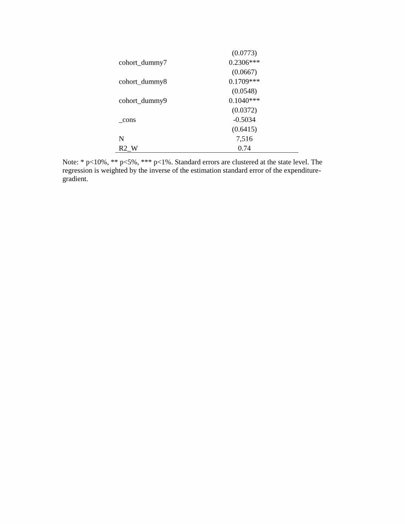
The first stage regression results (Appendix Table 1) show that 10 years of exposure to

reform reduces the expenditure-income gradient by about 1.04 standard deviations (s.d.=2.65

cents/dollar). This is consistent with Card and Payne (2002) which uses similar first-stage

regressions. It shows that exposure to SFR increases education equity by reducing the

expenditure-income gradient.


I use the predicted expenditure-income gradient in second stage regressions (table 8). The

baseline results show that a one standard deviation increase in expenditure-income gradient will

decrease the average college attendance rate of children with the lowest parent income by 2.87%,

and reduced the attendance slope by 2.42%. These effects are slightly smaller in the robustness

checks using dummy variables as instruments. Expenditure-income gradient shows no significant

income on the attendance rates of children with the highest parent income. OLS estimations,

when statistically significant, produce the opposite results with 2SLS, demonstrating the

importance of correcting the endogeneity bias of education expenditures.

VI. Conclusions

SFRs are built upon the premise that by increasing the equity of education expenditures,

the students’ outcome will depend less on their family backgrounds. Using commuting-zone-

level intergenerational mobility data for 10 birth cohorts, this study evaluates the long-term

effects of SFRs on college attendance rates, and tests the above premise. The results show that

SFRs have made a meaningful impact on low-income-student in terms of college attendance: for

children with lowest parent income, 10 years exposure to SFRs will increase their college

attendance rate by 5.72%, or a 35.2% relative increase from children with corresponding parent

income but did not experience SFRs. This impact decreases linearly with parent income rank,

and becomes statistically insignificant at about 70% parent income rank, but remains positive. As

a result, 10 years of exposure to SFRs decreases attendance rate gap between children with

lowest and highest parent income by 3.94%. These findings suggest that SFRs have improved the

college attendance equality by lifting up low income children. Event analysis shows that effect

increases in proportion to the duration of exposure to SFRs. However, when income rank is used

as the mobility measure, SFRs show no significant effects. This seems to contradict recent results

by Jackson et al. (2015), however it could also be the result of lower data quality in income ranks

compared to college attendance rates.

After quantifying the impacts of SFRs, this paper uses SFRs as natural experiments to

answer a broader question: to what degree, if any, intergenerational mobility is determined by

education equity? This paper finds that education equity has statistically significant effects, but

the size of effect depends on the mobility concept in question. If mobility is measured by the

chance of children from poorest families making it to college, then one standard deviation

increase in education equity can increase this chance by 2.87%, or a 17.7% relative increase; if

mobility is measured by the relative difference between the poorest and richest children, then one

standard deviation increase reduces this gap by 2.42%, which is only a 3.38% relative decrease.

For policymakers, it suggests that policies aimed at increasing education equity, such as SFRs,

can substantially benefit poor children but they alone are not enough to overcome the high

degree of existing inequalities.

Reference

Baicker, Katherine, and Nora Gordon. 2006. The effect of state education finance reform on total

local resources. Journal of Public Economics 90: 1519–35.

Bertrand, Marianne, Esther Duflo, and Sendhil Mullainathan. 2004. How much should we trust

difference-in-difference estimates. Article. Quarterly Journal of Economics 119: 249–75.

Card, David, and A Abigail Payne. 2002. School finance reform , the distribution of school

spending , and the distribution of student test scores. Journal of Public Economics 83: 49–

82.

Checchi, Daniele, Andrea Ichino, and Aldo Rustichini. 1999. More equal but less mobile?:

Education financing and intergenerational mobility in Italy and in the US. Journal of Public

Economics 74: 351–93.

Chetty, By Raj, Nathaniel Hendren, Patrick Kline, Emmanuel Saez, and Nicholas Turner. 2014.

Is the United States Still a Land of Opportunity ? Recent Trends in Intergenerational

Mobility. American Economic Review: Papers & Proceedings 104: 141–47.

Chetty, Raj, Nathaniel Hendren, Patrick Kline, and Emmanuel Saez. 2014. Where is the land of

Opportunity? The Geography of Intergenerational Mobility in the United States. Article.

The Quarterly Journal of Economics 129: 1553–1623.

Corcoran, Sean P., and William N. Evans. 2008. Equity, adequacy, and the evolving state role in

education finance. In Handbook of Research in Education Finance and Policy, edited by

Helen F. Ladd and Edward B. Fiske. New York: Routledge.

Downes, T A, and D N Figlio. 1998. School Finance Reforms, Tax Limits, and Student

Performance: Do Reforms Level Up or Dumb Down? Article. Discussion Papers.

Fischel, William A. 2006. The Courts and Public School Finance: Judge-Made Centralization

and Economic Research. Incollection. In , edited by E Hanushek and F Welch, 2:1279–

1325. Handbook of the Economics of Education. Elsevier.

Guryan, Jonathan. 2001. Does Money Matter? Regression-Discontinuity Estimates from

Education Finance Reform in Massachusetts. Techreport. Working Paper Series.

Hanushek, Eric A. 2003. The failure of input-based schooling policies. The Economic Journal

113: F64–98.

Hoxby, Caroline M. 2001. All School Finance Equalizations Are Not Created Equal. Article.

Quarterly Journal of Economics 116: 1189–1231.

Jackson, C Kirabo, Rucker C Johnson, and Claudia Persico. 2015. The Effects of School

Spending on Educational and Economic Outcomes: Evidence from School Finance

Reforms. NBER. Working Paper Series.

———. 2016. The Effects of School Spending on Educational and Economic Outcomes:

Evidence from School Finance Reforms. Article. The Quarterly Journal of Economics 131:

157–218.

Lafortune, Julien, Jesse Rothstein, and Diane Whitmore Schanzenbach. 2016. School finance

reform and the distribution of student achievement. Techreport.

Lynn, Zachary. 2011. Predicting the results of school finance adequacy lawsuits. Columbia

University.

Molloy, Raven, Christopher L Smith, and Abigail Wozniak. 2011. Internal migration in the

United States. Article. The Journal of Economic Perspectives 25. American Economic

Association: 173–96.

Murray, Sheila E, William N Evans, and Robert M Schwab. 1998. Education-Finance Reform

and the Distribution of Education Resources. American Economic Review 88: 789–812.

Papke, Leslie E. 2005. The effects of spending on test pass rates : evidence from Michigan.

Journal of Public Economics 89: 821–39.

Solon, Gary. 1992. Intergenerational income mobility in the United States. Article. The

American Economic Review. JSTOR, 393–408.

———. 2004. A Model of Intergenerational Mobility Variation over Time and Place. In

Generational Income Mobility in North America and Europe, edited by Miles Corak, 38–

47. Cambridge UK: Cambridge University Press.

Tables and Figures

Table 1. Court verdicts of school finance litigations and the subsequent reforms types.

State

Year of first

verdict against

SFRs

Year of first verdict

for SFRs Type of lawsuits

Alabama 1993 Adequacy

Alaska 1999 Adequacy

Arizona 1973 1994 Adequacy

Arkansas 1983 Equity

California 1986 1971 Equity

Colorado 1982

Connecticut 1985 1978 Equity

Delaware

District of Columbia

Florida 1996

Georgia 1981

Hawaii

Idaho 1975 1998 Adequacy

Illinois 1973

Indiana

Iowa

Kansas 1981 1972 Equity

Kentucky 2007 1989 Adequacy

Louisiana 1976

Maine 1995

Maryland 1972 2005 Adequacy

Massachusetts 2005 1993 Adequacy

Michigan 1973 1997 Adequacy

Minnesota 1971

Mississippi

Missouri 1993 Adequacy

Montana 1989 Equity

Nebraska 1993

Nevada

New Hampshire 1993 Adequacy

New Jersey 1973 Equity

New Mexico 1998 Equity

New York 1972 2003 Adequacy

North Carolina 1987 1997 Adequacy

North Dakota 1993

Ohio 1979 1997 Adequacy

Oklahoma 1987

Oregon 1976 2009 Adequacy

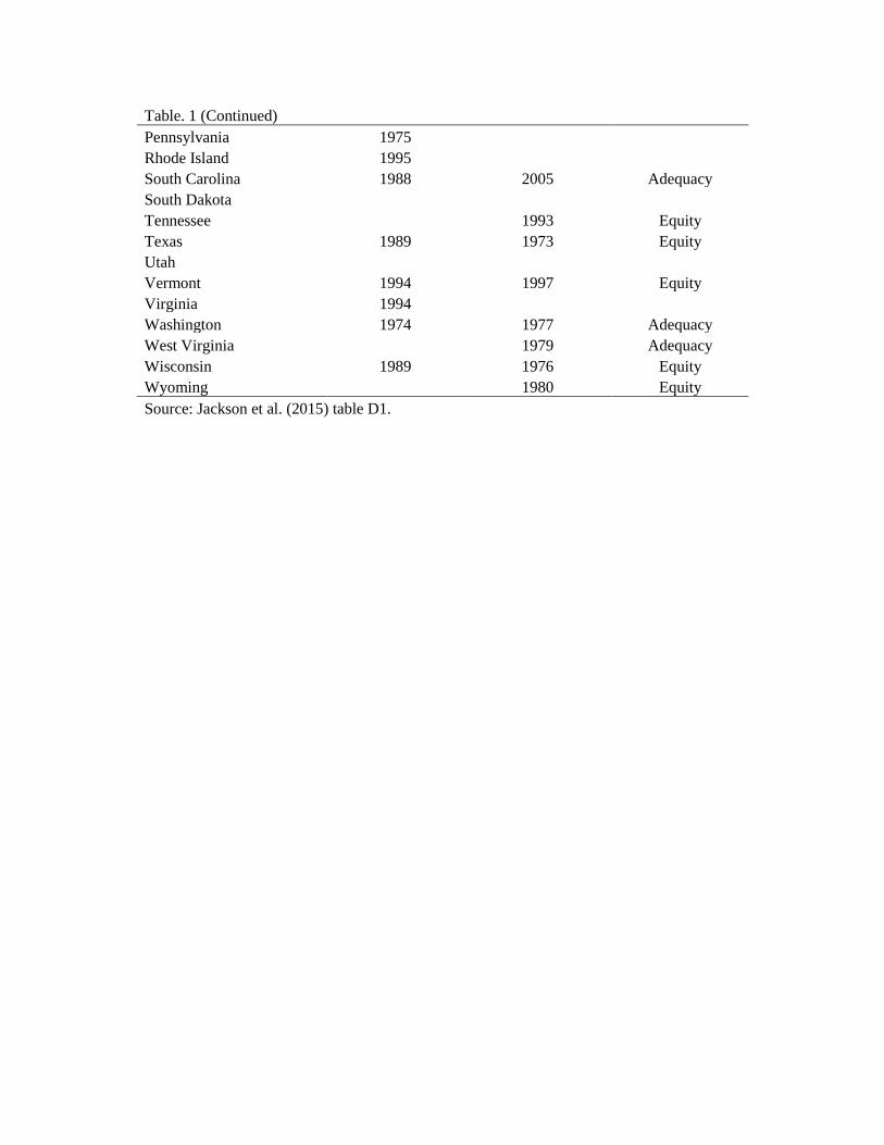
Table. 1 (Continued)

Pennsylvania 1975

Rhode Island 1995

South Carolina 1988 2005 Adequacy

South Dakota

Tennessee 1993 Equity

Texas 1989 1973 Equity

Utah

Vermont 1994 1997 Equity

Virginia 1994

Washington 1974 1977 Adequacy

West Virginia 1979 Adequacy

Wisconsin 1989 1976 Equity

Wyoming 1980 Equity

Source: Jackson et al. (2015) table D1.

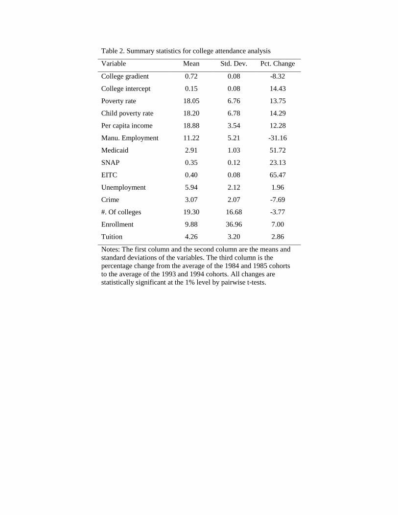
Table 2. Summary statistics for college attendance analysis

Variable Mean Std. Dev. Pct. Change

College gradient 0.72 0.08 -8.32

College intercept 0.15 0.08 14.43

Poverty rate 18.05 6.76 13.75

Child poverty rate 18.20 6.78 14.29

Per capita income 18.88 3.54 12.28

Manu. Employment 11.22 5.21 -31.16

Medicaid 2.91 1.03 51.72

SNAP 0.35 0.12 23.13

EITC 0.40 0.08 65.47

Unemployment 5.94 2.12 1.96

Crime 3.07 2.07 -7.69

#. Of colleges 19.30 16.68 -3.77

Enrollment 9.88 36.96 7.00

Tuition 4.26 3.20 2.86

Notes: The first column and the second column are the means and

standard deviations of the variables. The third column is the

percentage change from the average of the 1984 and 1985 cohorts

to the average of the 1993 and 1994 cohorts. All changes are

statistically significant at the 1% level by pairwise t-tests.

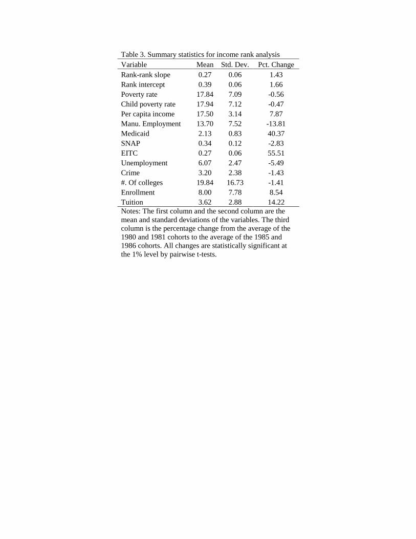
Table 3. Summary statistics for income rank analysis

Variable Mean Std. Dev. Pct. Change

Rank-rank slope 0.27 0.06 1.43

Rank intercept 0.39 0.06 1.66

Poverty rate 17.84 7.09 -0.56

Child poverty rate 17.94 7.12 -0.47

Per capita income 17.50 3.14 7.87

Manu. Employment 13.70 7.52 -13.81

Medicaid 2.13 0.83 40.37

SNAP 0.34 0.12 -2.83

EITC 0.27 0.06 55.51

Unemployment 6.07 2.47 -5.49

Crime 3.20 2.38 -1.43

#. Of colleges 19.84 16.73 -1.41

Enrollment 8.00 7.78 8.54

Tuition 3.62 2.88 14.22

Notes: The first column and the second column are the

mean and standard deviations of the variables. The third

column is the percentage change from the average of the

1980 and 1981 cohorts to the average of the 1985 and

1986 cohorts. All changes are statistically significant at

the 1% level by pairwise t-tests.

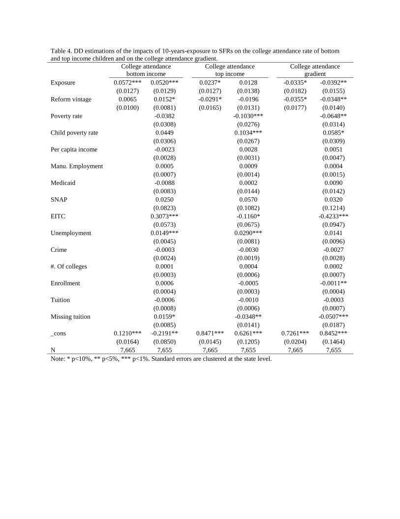
Table 4. DD estimations of the impacts of 10-years-exposure to SFRs on the college attendance rate of bottom

and top income children and on the college attendance gradient.

College attendance

bottom income

College attendance

top income

College attendance

gradient

Exposure 0.0572*** 0.0520*** 0.0237* 0.0128 -0.0335* -0.0392**

(0.0127) (0.0129) (0.0127) (0.0138) (0.0182) (0.0155)

Reform vintage 0.0065 0.0152* -0.0291* -0.0196 -0.0355* -0.0348**

(0.0100) (0.0081) (0.0165) (0.0131) (0.0177) (0.0140)

Poverty rate -0.0382 -0.1030*** -0.0648**

(0.0308) (0.0276) (0.0314)

Child poverty rate 0.0449 0.1034*** 0.0585*

(0.0306) (0.0267) (0.0309)

Per capita income -0.0023 0.0028 0.0051

(0.0028) (0.0031) (0.0047)

Manu. Employment 0.0005 0.0009 0.0004

(0.0007) (0.0014) (0.0015)

Medicaid -0.0088 0.0002 0.0090

(0.0083) (0.0144) (0.0142)

SNAP 0.0250 0.0570 0.0320

(0.0823) (0.1082) (0.1214)

EITC 0.3073*** -0.1160* -0.4233***

(0.0573) (0.0675) (0.0947)

Unemployment 0.0149*** 0.0290*** 0.0141

(0.0045) (0.0081) (0.0096)

Crime -0.0003 -0.0030 -0.0027

(0.0024) (0.0019) (0.0028)

#. Of colleges 0.0001 0.0004 0.0002

(0.0003) (0.0006) (0.0007)

Enrollment 0.0006 -0.0005 -0.0011**

(0.0004) (0.0003) (0.0004)

Tuition -0.0006 -0.0010 -0.0003

(0.0008) (0.0006) (0.0007)

Missing tuition 0.0159* -0.0348** -0.0507***

(0.0085) (0.0141) (0.0187)

_cons 0.1210*** -0.2191** 0.8471*** 0.6261*** 0.7261*** 0.8452***

(0.0164) (0.0850) (0.0145) (0.1205) (0.0204) (0.1464)

N 7,665 7,655 7,665 7,655 7,665 7,655

Note: * p<10%, ** p<5%, *** p<1%. Standard errors are clustered at the state level.

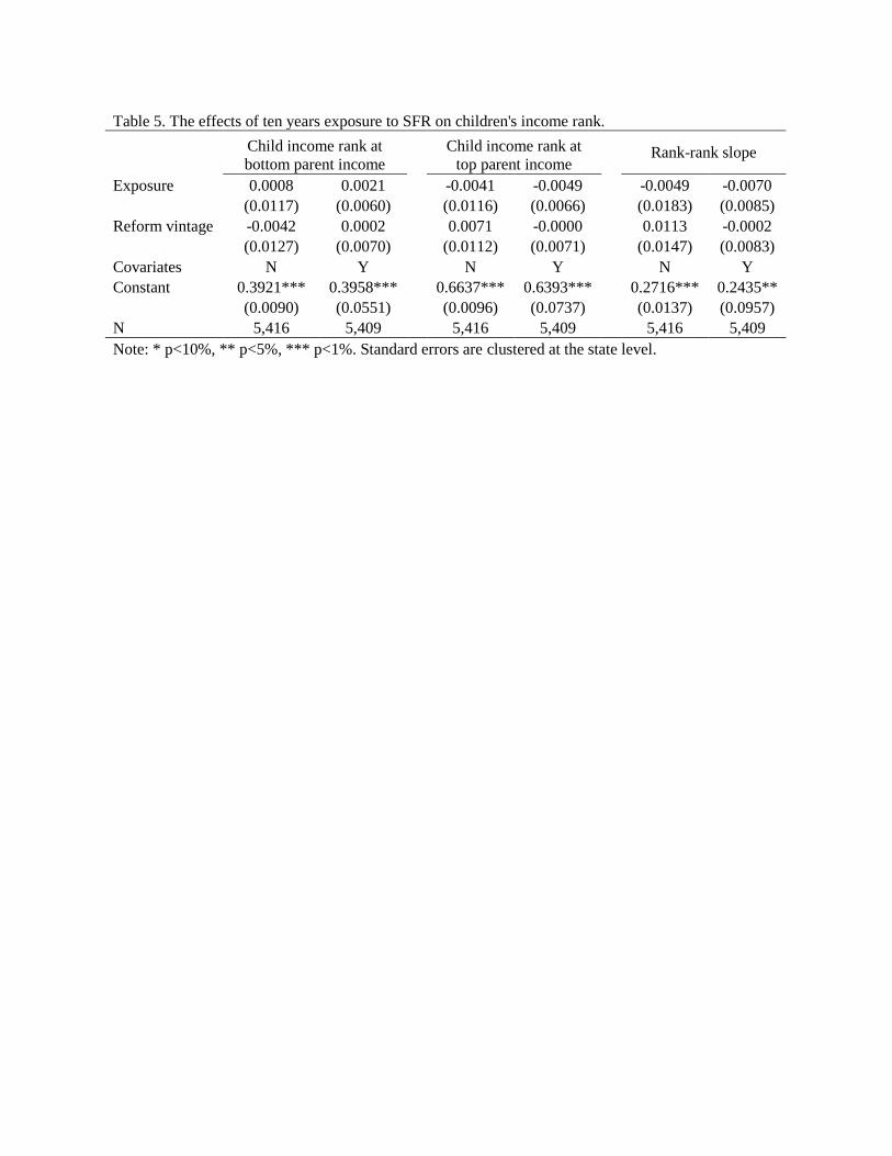
Table 5. The effects of ten years exposure to SFR on children's income rank.

Child income rank at

bottom parent income

Child income rank at

top parent income Rank-rank slope

Exposure 0.0008 0.0021 -0.0041 -0.0049 -0.0049 -0.0070

(0.0117) (0.0060) (0.0116) (0.0066) (0.0183) (0.0085)

Reform vintage -0.0042 0.0002 0.0071 -0.0000 0.0113 -0.0002

(0.0127) (0.0070) (0.0112) (0.0071) (0.0147) (0.0083)

Covariates N Y N Y N Y

Constant 0.3921*** 0.3958*** 0.6637*** 0.6393*** 0.2716*** 0.2435**

(0.0090) (0.0551) (0.0096) (0.0737) (0.0137) (0.0957)

N 5,416 5,409 5,416 5,409 5,416 5,409


Table 6. Robustness check with court decisions upholding the status quo.

College attendance

bottom income

College attendance

top income

College attendance

gradient

Exposure 0.0555*** 0.0500*** 0.0234* 0.0124 -0.0321 -0.0377**

(0.0130) (0.0127) (0.0134) (0.0140) (0.0193) (0.0163)

Upheld -0.0188 -0.0199 -0.0025 -0.0047 0.0164 0.0153

(0.0318) (0.0346) (0.0216) (0.0212) (0.0308) (0.0253)

Reform vintage 0.0050 0.0136* -0.0293* -0.0200 -0.0342* -0.0336**

(0.0105) (0.0080) (0.0170) (0.0135) (0.0186) (0.0146)


Constant 0.1356*** -0.2090** 0.8490*** 0.6285*** 0.7134*** 0.8375***

(0.0313) (0.0889) (0.0261) (0.1227) (0.0379) (0.1480)

N 7,665 7,655 7,665 7,655 7,665 7,655


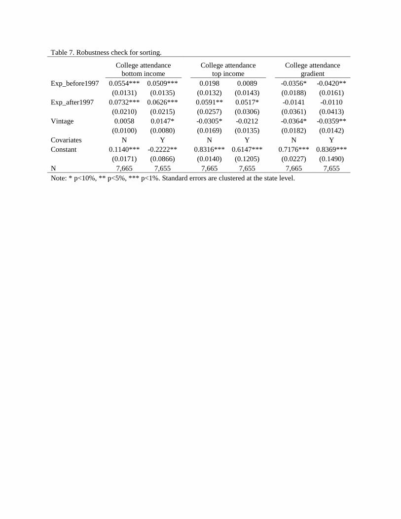
Table 7. Robustness check for sorting.

College attendance

bottom income

College attendance

top income

College attendance

gradient

Exp_before1997 0.0554*** 0.0509*** 0.0198 0.0089 -0.0356* -0.0420**

(0.0131) (0.0135) (0.0132) (0.0143) (0.0188) (0.0161)

Exp_after1997 0.0732*** 0.0626*** 0.0591** 0.0517* -0.0141 -0.0110

(0.0210) (0.0215) (0.0257) (0.0306) (0.0361) (0.0413)

Vintage 0.0058 0.0147* -0.0305* -0.0212 -0.0364* -0.0359**

(0.0100) (0.0080) (0.0169) (0.0135) (0.0182) (0.0142)


Constant 0.1140*** -0.2222** 0.8316*** 0.6147*** 0.7176*** 0.8369***

(0.0171) (0.0866) (0.0140) (0.1205) (0.0227) (0.1490)

N 7,665 7,655 7,665 7,655 7,665 7,655


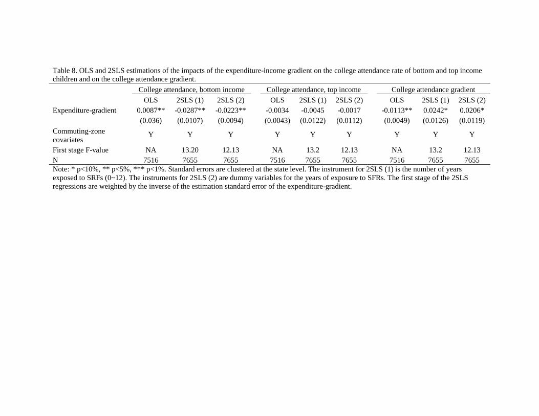
Table 8. OLS and 2SLS estimations of the impacts of the expenditure-income gradient on the college attendance rate of bottom and top income

children and on the college attendance gradient.

College attendance, bottom income College attendance, top income College attendance gradient

OLS 2SLS (1) 2SLS (2) OLS 2SLS (1) 2SLS (2) OLS 2SLS (1) 2SLS (2)

Expenditure-gradient 0.0087** -0.0287** -0.0223** -0.0034 -0.0045 -0.0017 -0.0113** 0.0242* 0.0206*

(0.036) (0.0107) (0.0094) (0.0043) (0.0122) (0.0112) (0.0049) (0.0126) (0.0119)

Commuting-zone

covariates Y Y Y Y Y Y Y Y Y

First stage F-value NA 13.20 12.13 NA 13.2 12.13 NA 13.2 12.13

N 7516 7655 7655 7516 7655 7655 7516 7655 7655

Note: * p<10%, ** p<5%, *** p<1%. Standard errors are clustered at the state level. The instrument for 2SLS (1) is the number of years

exposed to SRFs (0~12). The instruments for 2SLS (2) are dummy variables for the years of exposure to SFRs. The first stage of the 2SLS

regressions are weighted by the inverse of the estimation standard error of the expenditure-gradient.

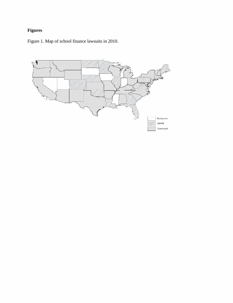
Figures

Figure 1. Map of school finance lawsuits in 2010.

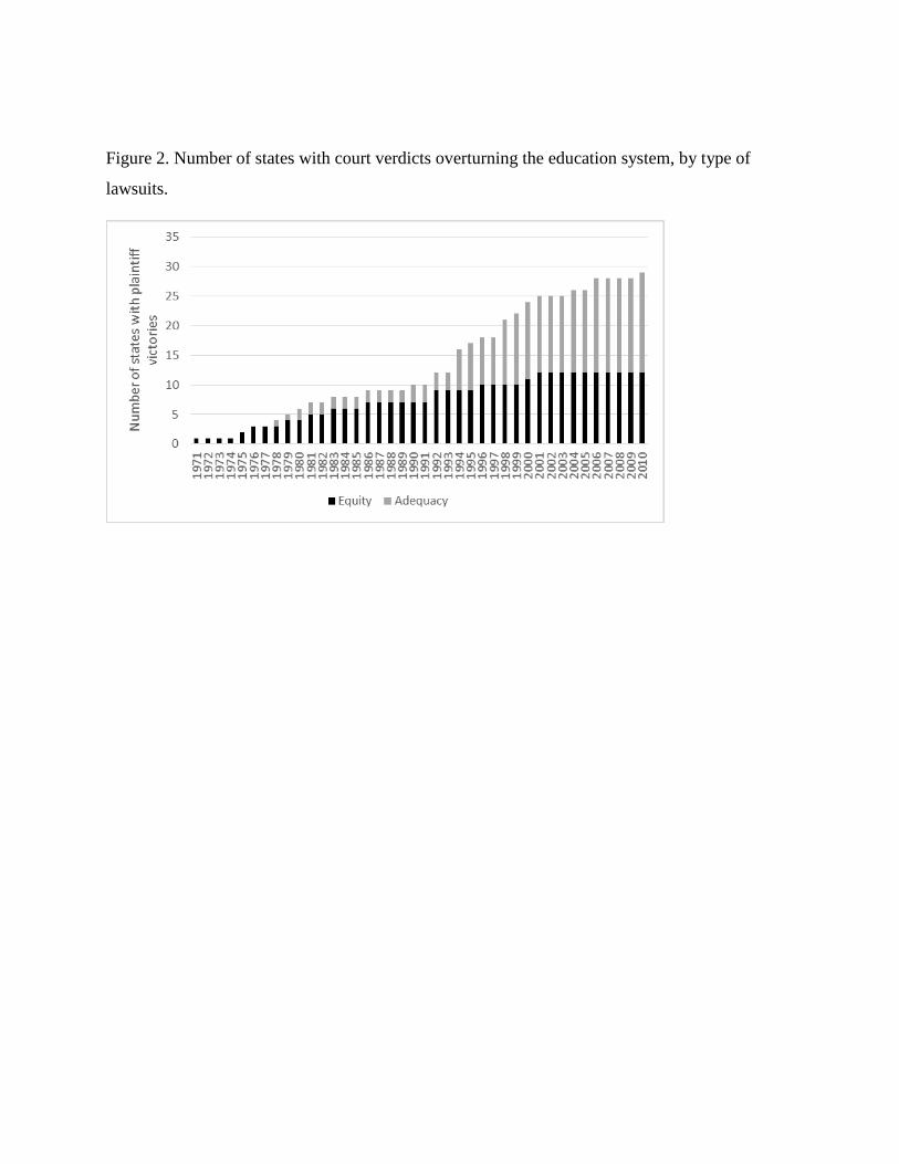
Figure 2. Number of states with court verdicts overturning the education system, by type of

lawsuits.

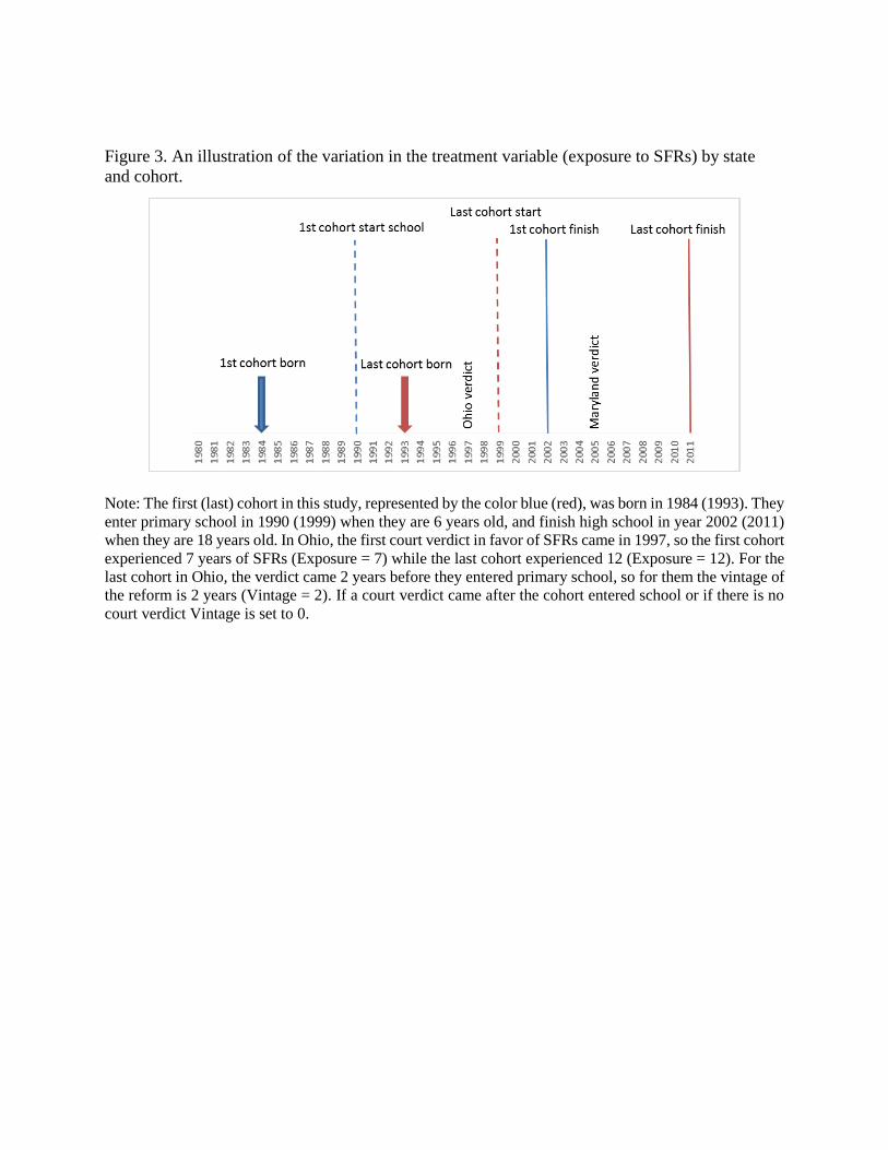
Figure 3. An illustration of the variation in the treatment variable (exposure to SFRs) by state

and cohort.

Note: The first (last) cohort in this study, represented by the color blue (red), was born in 1984 (1993). They

enter primary school in 1990 (1999) when they are 6 years old, and finish high school in year 2002 (2011)

when they are 18 years old. In Ohio, the first court verdict in favor of SFRs came in 1997, so the first cohort

experienced 7 years of SFRs (Exposure = 7) while the last cohort experienced 12 (Exposure = 12). For the

last cohort in Ohio, the verdict came 2 years before they entered primary school, so for them the vintage of

the reform is 2 years (Vintage = 2). If a court verdict came after the cohort entered school or if there is no

court verdict Vintage is set to 0.

Figure 4. The impacts of SFRs across the parent income spectrum.

Note: College attendance rates are calculated for 10% intervals of parent income ranks using the intercepts

and slopes published by CHKS. Regressions in table 3 (with covariates) are estimated for each parent

income rank percentile. The coefficient estimates are represented by the solid line and 90% confidence

intervals are represented by the dashed lines. The y-axis represents the change in college attendance rate

caused by 10 years of exposure to SFRs.

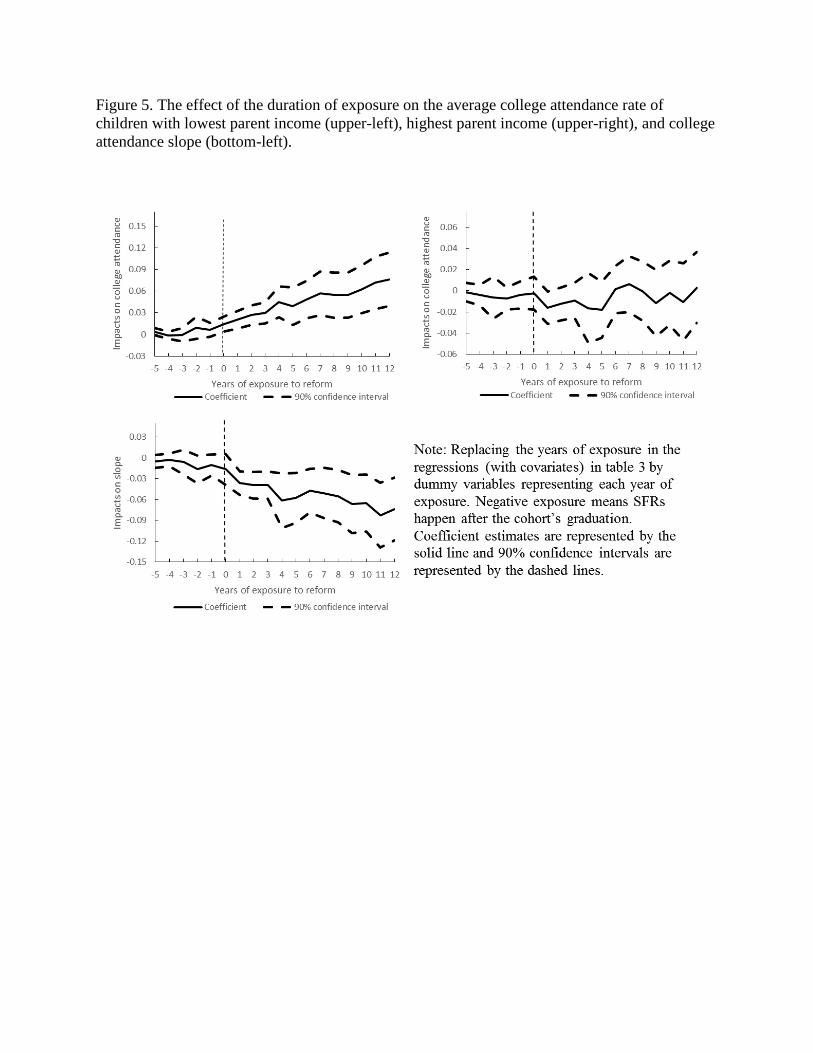
Figure 5. The effect of the duration of exposure on the average college attendance rate of

children with lowest parent income (upper-left), highest parent income (upper-right), and college

attendance slope (bottom-left).

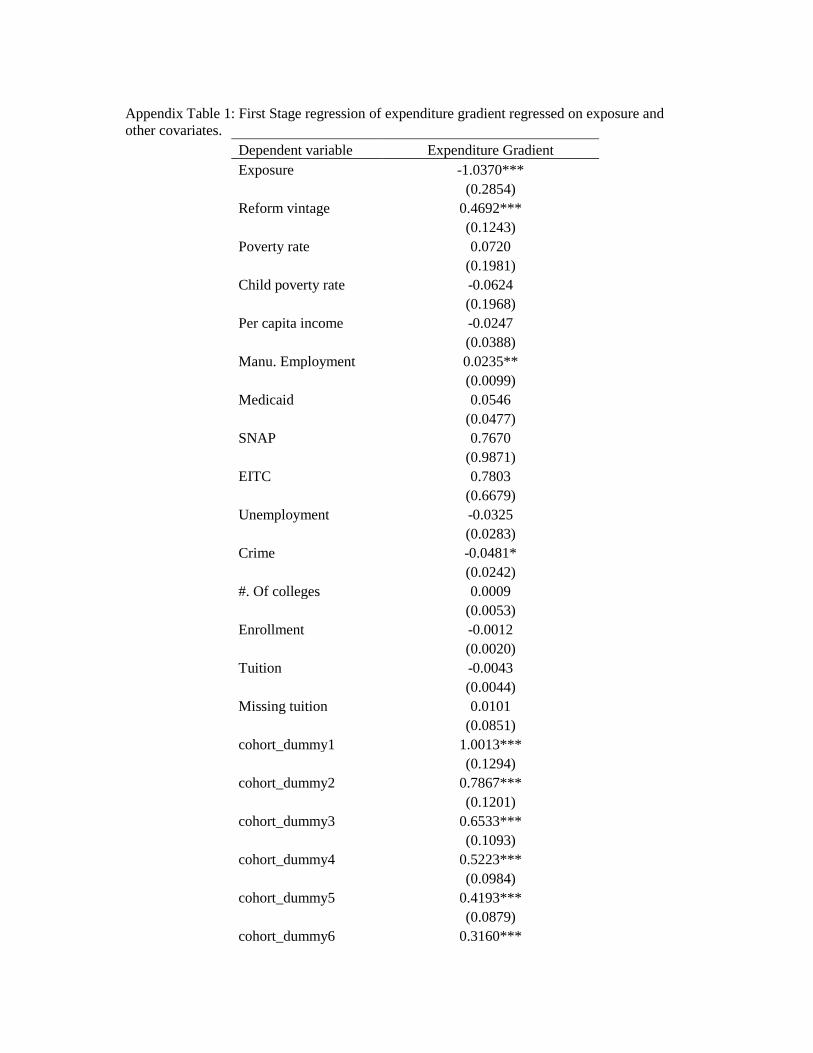
Appendix Table 1: First Stage regression of expenditure gradient regressed on exposure and

other covariates.

Dependent variable Expenditure Gradient

Exposure -1.0370***

(0.2854)

Reform vintage 0.4692***

(0.1243)

Poverty rate 0.0720

(0.1981)

Child poverty rate -0.0624

(0.1968)

Per capita income -0.0247

(0.0388)

Manu. Employment 0.0235**

(0.0099)

Medicaid 0.0546

(0.0477)

SNAP 0.7670

(0.9871)

EITC 0.7803

(0.6679)

Unemployment -0.0325

(0.0283)

Crime -0.0481*

(0.0242)

#. Of colleges 0.0009

(0.0053)

Enrollment -0.0012

(0.0020)

Tuition -0.0043

(0.0044)

Missing tuition 0.0101

(0.0851)

cohort_dummy1 1.0013***

(0.1294)


(0.1201)


(0.1093)


(0.0984)


(0.0879)


(0.0773)


(0.0667)


(0.0548)


(0.0372)

_cons -0.5034

(0.6415)

N 7,516

R2_W 0.74

Note: * p<10%, ** p<5%, *** p<1%. Standard errors are clustered at the state level. The

regression is weighted by the inverse of the estimation standard error of the expenditure-

gradient.

Documents

Education equity and intergenerational mobility: Quasi ... · education expenditure and parent income should lead to higher intergenerational mobility. Placing the magnitudes of these