Education and Saving:The Long-Term Effects of High School

Financial Curriculum Mandates

by

B. Douglas BernheimStanford University

National Bureau of Economic Research

Daniel M. GarrettCornerstone Research

Dean M. MakiBoard of Governors of the Federal Reserve System

June 1997

______________________________________________________________________________We are grateful to the National Science Foundation (grant number SBR94-009043 and SBR95-11321),Merrill Lynch & Co., Inc., and an anonymous private foundation for financial support, and to Merrill Lynch& Co., Inc., for sponsoring the collection of the data on which this study is based. We would like to thankPeter Brady, Martha Starr-McCluer, John Pencavel, Jim Poterba, and Jonathan Skinner for helpful comments,Heather Nevin for excellent research assistance, and Hayden Green for valuable conversations concerning theconsumer education movement. The views expressed in this paper are those of the authors and do notnecessarily reflect the positions of any organization.

Abstract

Over the last forty years, the majority of states have adopted consumer education policies, and a

sizable minority have specifically mandated that high school students receive instruction on topics related to

household financial decision-making (budgeting, credit management, saving and investment, and so forth). In

this paper, we attempt to determine whether the curricula arising from these mandates have had any

discernable effect on adult decisions regarding saving. Using a unique household survey, we exploit the

variation in requirements both across states and over time to identify the effects of interest. The evidence

indicates that mandates have significantly raised both exposure to financial curricula and subsequent asset

accumulation once exposed students reached adulthood. These effects appear to have been gradual rather

than immediate -- a probable reflection of implementation lags.

See Alexander (1979), Highsmith (1989), and Scott (1990) for a detailed description of these mandates. A more concise1

summary is presented in section 2 of this paper.

For example, legislation in the state of Georgia states: “Each citizen should have the skills and knowledge to be an2

informed consumer in order to use available resources in an efficient and beneficial manner” (Alexander, 1989).

The Head Start program is a good example; see e.g. the discussion in Currie and Thomas (1995).3

1

1. Introduction

Between 1957 and 1985, 29 states adopted legislation mandating some form of “consumer”

education in secondary schools. In 14 cases, these measures specifically required coverage of topics relevant

to household financial decision-making, from budgeting, credit management, and balancing checkbooks to

compound interest and other investment principles. The objective of these curriculum mandates was to1

equip students with practical decision-making skills that would prove useful in their adult lives.2

Should one expect high school consumer/financial curriculum mandates to be effective in achieving

this objective? There are reasons for both optimism and pessimism. On the one hand, there is some evidence

that poor financial decisions frequently result, at least to some degree, from a failure to appreciate economic

vulnerabilities (Bernheim, 1994, 1995). Education could alleviate this problem by contributing pertinent

knowledge and/or specific decision-making skills. Early financial education may also increase comfort and

familiarity with financial matters, thereby removing psychological barriers that impede proper decision-

making. By way of analogy, the early acquisition of computer literacy appears to have a long-term effect on

an individual’s general level of comfort with computers. On the other hand, long-run effects of targeted

educational initiatives have been difficult to detect in other contexts. Broad mandates may have little real3

influence on curriculum content, classroom treatment of critical financial topics may be cursory, and/or

students may fail to take the material seriously. Of course, all of these considerations, both positive and

negative, are speculative. Virtually nothing is known about the long-term behavioral effects of financial

To the extent previous studies have explored the effects of consumer/economic education, they have focused on the short-4

term, and have usually examined measures of knowledge or attitudes rather than behavior. See e.g. Peterson (1992), Soper andBrenneke (1981), Kohen and Kipps (1979), and Langrehr (1979). One exception is Fast, Vosburgh, and Frisbee (1989), whoanalyzed the effects of consumer education on consumer search.

2

education in secondary schools.4

In this paper, we attempt to determine whether the curricula arising from high school financial

education mandates have had any discernable effect on adult financial decision-making. Obviously, this issue

has many dimensions, including the adequacy of saving, the appropriate management of credit, and prudent

portfolio allocation. While we are interested in all of these dimensions, we focus here only on the first (the

adequacy of saving). This focus is motivated in part by the widespread (though certainly not universal)

concern that the typical American saves too little (see e.g. Bernheim, 1991, 1996a). Rather than develop a

formal model to measure the adequacy of saving, we simply ask whether exposure to a high school financial

curriculum leads to higher saving as an adult.

Our analysis is based on a unique cross-sectional household survey fielded in the Fall of 1995,

which, among other things, solicited the state in which the respondent attended high school, as well as

recollections concerning exposure to financial education. In attempting to detect the effects of curriculum

mandates, we are aided by the fact that some states never adopted these programs, and that the others adopted

them at different times. Our analysis is based on comparisons both across states and over time -- using the

non-adopting states as a benchmark, we investigate whether the establishment of a mandate coincided with a

departure from this benchmark among the affected cohorts.

We begin our investigation by studying exposure to financial education. There is no indication that

mandates are correlated with pre-existing inclination to offer, require, or take financially oriented courses.

Students in the typical state that enacted a mandate were no more likely, prior to the mandate, to have been

exposed to financial education than were students in the typical state that never enacted a mandate. However,

differences in reported exposure rates do appear after mandates are introduced, and increase steadily with the

For recent surveys of this literature, see Bernheim (1996b), Hubbard and Skinner (1996), Poterba, Venti, and Wise5

(1996), and Gale and Scholz (1996).

3

passage of time. This suggests that the effect of a mandate is gradual, perhaps reflecting lags associated with

curriculum development, adoption, and compliance.

Data on self-reported rates of saving mirror this pattern extremely closely: there are no differences

(either in levels or age-trends) across states before the adoption of a mandate, but there is a steady and

significant divergence after adoption, in the expected direction. A somewhat different pattern is predicted for

the accumulation of net wealth; however, the basic predictions (no systematic difference from the benchmark

among those too old to have been exposed, significant difference for those young enough to have been

exposed) find considerable support in the data. Overall, the evidence suggests that adoption was not

systematically related to pre-existing preferences -- that it is probably best regarded as exogenous.

Irrespective of that issue, specifications that control for systematic differences across states provide strong

indications that mandates not only increased exposure to financial education, but also systematically altered

adult behavior by stimulating greater saving.

Although this is, to our knowledge, the first study to examine the effects of secondary school

education on adult financial decisions, it is certainly related to several strands of the literature. One pertinent

strand is concerned with the evaluation of policies to increase saving. There is an extensive literature on tax

incentives, which reaches somewhat ambiguous conclusions. There is also a smaller, but more closely5

related literature that investigates the relation between saving and education. Much of this is anecdotal and/or

inconclusive. For example, although there is some indication that the post-War increase in saving by

Japanese households may have been at least partially attributable to an extensive educational and promotional

campaign, there are other competing explanations for the same phenomenon (see Bernheim, 1991, or Central

Council for Savings Promotion, 1981). Likewise, correlations between an individual’s general level of

educational attainment and his or her rate of saving (documented by Bernheim and Scholz, 1993, and by

4

Hubbard, Skinner, and Zeldes, 1995) may be attributable to other related factors, such as rates of time

preference. A more promising branch of this literature has focused specifically on the behavioral effects of

retirement education in the workplace (Bernheim and Garrett, 1996, Bayer, Bernheim, and Scholz, 1996,

Bernheim, 1996c, Clark and Schieber, 1996, and Yakoboski, 1996). Subject to some qualifications, these

studies have identified significant effects on saving. The growing body of evidence concerning the effects of

education on financial decision-making has recently led the Department of Labor to launch “a national

pension education program aimed at drawing the attention of American workers to the importance of taking

personal responsibility for their retirement security” (Berg, 1995, p. 2).

The paper is related also to the more general literature on the returns to education. Much of this

literature has focused on the relation between wages and either training or schooling. A central issue in this

literature concerns the likelihood that both of these variables are related to some underlying unobservable

characteristic, such as ability (see e.g. Ashenfelter, 1978, Lalonde, 1986, or Card, 1995). Causal inferences

about the effects of education are potentially misleading unless they are derived from sources of variation in

education that are plausibly exogenous. Naturally, identical issues arise in the context of the current

investigation. In certain respects, our approach is similar in spirit to that of Angrist and Krueger (1991,

1995), who attempt to infer the effects of secondary education from variation in state mandatory schooling

laws, which they treat as exogenous. Notably, since financial curriculum mandates vary both across states

and over time, our investigation does not require us to make a similar assumption concerning exogeneity.

Instead, we investigate whether the imposition of mandates correlates with changes in behavior. This general

strategy has been used in a variety of other contexts; for example, Hoxby (1996) identifies the effect of

teachers’ unionization on educational performance by studying the variation in pertinent state laws.

The paper is organized as follows. Section 2 summarizes the history and content of state financial

education mandates. Section 3 describes the household survey data used in our analysis. Section 4 examines

the effects of mandates on exposure to financial education. Section 5 studies the effects of mandates on rates

See Bannister and Monsma (1982) for a complete classification of the various concepts that are included in the field of6

consumer education.

See National Institute for Consumer Education (1994) for an example of a teaching guide for personal finance education.7

5

of saving and wealth accumulation. Section 6 concludes.

2. State Financial Curriculum Mandates

The financial education mandates analyzed in this paper are a subset of the larger set of consumer

education mandates. Consumer education covers a wide range of topics. Alexander (1979) and Scott (1990)6

refer to four sub-fields of consumer education: Consumer decision-making, economics, personal finance, and

consumer rights and responsibilities.

Consumer decision-making includes instruction in assessing the consumer's goals and needs, as well

as training in the decision-making skills used to meet the goals and needs. This area often focuses on factors

that should be considered in choosing among various goods and services, such as prices, product features,

warranties, and operation and repair costs. Consumer decision-making also may cover the analysis of

advertising messages and product labels. Economics, the second area of consumer education, typically deals

with concepts such as the allocation of scarce resources, the roles of consumers, producers, and government

in an economic system, the principles of supply and demand, and the role of prices in a market system. The

third area, personal finance, may cover household budgeting, money management, saving and investing, and

the use of credit. The saving and investing portion of such a course may offer discussion on various types of

financial instruments, the relationship between risk and return, and the role of inflation, taxes and

diversification in portfolio choice. Finally, the area of consumer rights and responsibilities offers instruction7

on consumer protection laws and regulations, along with redress mechanisms available to consumers.

Thirty seven states have policies that encourage or require instruction in consumer education, or have

had such policies in the past. Some policies merely “encourage” consumer education to be taught. Other

For more information on policies for each state, see Alexander (1979), Joint Council on Economic Education (1989) and8

the National Coalition for Consumer Education (1990). There are some discrepancies between sources, particularly betweenAlexander (1979) and later sources. These discrepancies may be due to differences in interpretations of survey questions or to policychanges after 1978. When possible, state school administrators were questioned about discrepancies. If discrepancies could not bereconciled, Alexander (1979) was used as the definitive source, on the grounds that more recent sources are less likely to haveclassified state policies correctly during the time period that is of greatest relevance to this study. There is some remaining ambiguityabout the correct classification of Wisconsin, but our results are not particularly sensitive to the reclassification of this state. Policiesalso may have changed since 1990, but such changes would not affect the results in this paper because affected households would betoo young to be included in the sample.

6

states have mandates covering consumer education, although such mandates vary in scope, from requiring

state education agencies to develop and distribute materials on consumer education to local districts to

imposing requirements at the local level by requiring each district to offer some form of consumer education.

Also, a number of states specifically mandate that each student receive instruction in a consumer education

course; some of these states require a separate course, while others allow schools to integrate consumer

education into existing courses.

The analysis in this paper will focus on the mandates that require all students to receive instruction in

consumer education. Because they are universal, these types of mandates seem the most likely to affect

behavior. Table 1 summarizes consumer education policies in the 50 states and the District of Columbia.

The table indicates whether a state has adopted a consumer education policy, the first graduating class to be

affected by the policy, and whether the policy mandates that all public school students receive instruction in

consumer education, or specifically in personal finance education. The earliest policy was instituted by

Nevada in 1957, and most of the policies were implemented in the 1970s. Students are required to receive8

consumer education in 29 states, while in 14 states students specifically are required to receive instruction in

personal finance.

This paper attempts to measure the effect of mandated consumer education policies on saving and

wealth accumulation later in life. A potential problem with assessing the effect of mandates on saving

behavior is that mandates may be endogenous, if states whose residents had a high preference for saving were

the same states that enacted mandates. This type of endogeneity seems unlikely for several reasons.

See Bannister (1996) for a history of consumer education in the U.S., and Mayer (1989) for a history of the broader9

consumer movement.

Conversations with consumer education experts in Illinois indicated that keys to enactment of its consumer education10

legislation were highly publicized fraud cases as well as the political skill of key legislators.

For additional background on the passage and development of consumer education policies and programs, see Langrehr11

and Mason (1977), or Herrman (1982).

7

Consumer education mandates seem to be an outgrowth of the broader consumer movement of the 1960s and

1970s that is most closely associated with Ralph Nader. Few consumer education laws focused mainly on9

personal finance. More commonly, the laws were directed at all four of the areas mentioned above.

Moreover, Mayer (1989) argues for the importance of sound tactical strategy by lobbying groups and the

preferences of key legislators as keys for the passage of consumer laws, rather than public opinion more

broadly defined.

When public opinion is important to enactment of consumer legislation, it is usually associated with

outrage over a particular event that damaged consumers in some way. The importance of lobbying groups10

as opposed to broad public opinion also was borne out in a survey of chief state school administrators (Scott,

1990). When asked "Which group is most likely to discuss consumer education initiatives?" 41 percent of

the school administrators indicated education professionals such as teachers, school administrators, and their

staffs; 39 percent indicated the business community; and only 10 percent indicated that parents or students

were the most likely to discuss consumer education initiatives. There is little reason to believe that the

preferences of politically active education professionals or business leaders are generally representative of

household preferences in a given state. Further evidence is provided by Ford (1977), who finds that states

that passed consumer education legislation were not statistically significantly different from other states in

income, retail sales, or the proportion of residents who graduated from high school. Thus, it seems unlikely

that passage of a consumer education policy in a particular state was correlated with the pre-mandate

financial behavior of the state's households. Nevertheless, the empirical analysis in this paper controls for11

differences in pre-mandate saving behavior between states where a mandate was imposed and other states to

8

check whether this intuition is borne out statistically.

3. Survey Data

To examine the effects of high school financial curriculum mandates, one requires a household

survey data set with several characteristics. First, the data must be recent. Since most workers are on the

steepest portions of their earnings trajectories during their 20s and early 30s, one generally observes

relatively little saving (and relatively little divergence of saving across groups) prior to the mid-30s. As

indicated in table 1, many states did not adopt mandates until the mid-1970s. An individual who was

exposed to financial education in 1976 at the age of 16 would not have reached age 35 until 1995. Second, to

assess exposure to financial education, the survey should solicit the state in which each individual attended

high school. If mobility across states is sufficiently low, then current state of residence might be a reasonable

proxy. Direct measures of exposure to financial education (based on appropriately worded questions) are

also desirable. Third, the survey must collect information on financial choices (saving and wealth), as well as

the usual array of economic and demographic data (e.g. earnings, age, and so forth).

Unfortunately, there is currently no publicly available data set that satisfies these criteria. Consider,

for example, the Survey of Consumer Finances (SCF). When this project was conducted, data from the 1992

SCF were available, but the 1995 data had not yet been released. SCF respondents were not asked directly

about exposure to financial education, and the survey did not solicit the state in which the respondent

attended high school. While state of current residence is recorded in the survey, in practice this information is

withheld from the public to ensure confidentiality. Furthermore, the use of current state in place of high

school state would yield a poorer measure of exposure to mandates, and would thereby bias our analysis

against the finding that mandates affect behavior. Similar problems arise for other data sources, such as the

Survey of Income and Program Participation, and the Panel Study of Income Dynamics. Thus, to address the

nexus of issues identified in section 1, it was necessary to collect new data.

The survey was designed in cooperation with the first author of this paper, and fielded for Merrill Lynch by the Luntz12

Research Companies.

Respondents who terminated their interviews before completion of the survey are not included in this sample.13

Respondents were asked separately about the value of financial assets, houses, other real property, business interests, and14

debt.

Respondents were asked to identify the type of pension (defined benefit, voluntary tax-deferred salary reduction plan, or15

other defined contribution), and to provide total assets for defined contribution plans.

Each household was asked to estimate the fraction of take-home pay that it saved on its own behalf (not including16

reinvested capital income or employer contributions to retirement accounts).

If they lived in more than one state during high school, they were asked to name the state in which they lived the longest.17

The survey did not elicit similar information concerning spouses.18

9

The first author of this paper has directed an ongoing project, sponsored by Merrill Lynch, Inc., to

monitor the adequacy of personal saving through annual household surveys (see Bernheim, 1996a). For the

fall of 1995, the survey instrument was expanded to cover several new topics, including high school financial

education. Data were collected during the month of November, 1995 from a nationally representative12

sample of respondents between the ages of 30 and 49. This age-specific focus is appropriate for the current

study, since these are the age groups that experienced the transition to financial curriculum mandates in many

states. A total of 2,000 surveys were completed. The survey gathered standard economic and demographic13

information, including household assets and liabilities, earnings of respondent and spouse, total household14

income, various aspects of pension coverage, employment status, gender, marital status, age, ethnic group,15

education, and household composition. It also solicited self-reported rates of saving, as well as information16

on a variety of less standard topics, such as childhood influences of potential relevance to future financial

decisions (e.g. parental attitudes toward saving, and the fraction of the respondent’s high school class that

attended college).

Most importantly, the Merrill Lynch survey specifically asked respondents to identify the state in

which they attended high school, and it solicited information concerning exposure to financial education. 17 18

This information was gathered in three steps. First, respondents were asked if, in high school, they took any

When an individual reported that the value of a variable fell within a given bracket, we imputed the value by taking the19

median of the variable for the subset of individuals who provided numerical answers within the same bracket. Within brackets,additional variables (e.g. demographics) had little predictive power, and therefore were not used to improve imputations.

For the remaining 14 percent of the sample, we imputed earnings based on a regression of earnings on a third degree20

polynomial in age, years of education, gender, ethnicity dummies, marital status, and employment status.

10

courses dealing with household finances, consumer education, or economics. Those who answered “yes”

were then asked whether any of these courses specifically covered topics that had to do with household

finances, such as the use of budgets, credit, savings accounts, checking accounts, and so forth. Each

respondent who answered “yes” to this second question was then asked whether any of these courses were

required by his or her school. Issues concerning the accuracy of these recollections are considered below,

where pertinent.

One potential problem is that the survey was administered by telephone. While telephone interviews

are usually regarded as less reliable than face-to-face interviews, the survey was designed to achieve a high

level of compliance and to assure accuracy. Questions were sequenced according to their degree of

invasiveness. This permitted interviewers to establish credibility, to place respondents at ease, and to engage

them in the survey process. Invasive questions concerning assets and earnings were deferred until later in the

survey, and the most innocuous of these (for example, the household’s estimated rate of saving) were placed

before the most problematic ones (primarily those designed to elicit asset holdings). Bracketed information

was solicited from those who were unable or refused to give numerical answers, and provided a basis for

making imputations. Response rates were relatively high; for example, 74 percent of respondents provided19

numerical information on annual earnings, and another 12 percent provided bracketed information. 20

Tables 2 and 3 contain summary statistics based on the survey data. Since the reliability of telephone

interviews is open to question, it is useful to compare these numbers to those drawn from other recognized

data sources. For benchmarks, the reader is referred to a study by the Congressional Budget Office (1993),

which tabulated statistics for 25-34 and 35-44 year olds, based on the 1989 Survey of Consumer Finances

and the 1990 Current Population Survey (see also Bernheim and Garrett, 1996, who compare the 1994

In addition to the patterns displayed in the table, measured earnings also vary in the expected manner with education and21

ethnicity.

11

Merrill Lynch survey to these benchmarks). Generally, the data conform reasonably well to these

benchmarks. The fraction of respondents who are married and the fraction who are homeowners are a bit

high (by perhaps five or six percentage points), but this is understandable given that such households are

probably relatively easy to reach by telephone. African Americans are also underrepresented in the survey.

Once one accounts for these patterns of oversampling and undersampling, it becomes apparent that median

income and wealth are of the right magnitudes. The wealth distribution also exhibits the usual thick upper

tail. Wealth and earnings also vary in the appropriate manner across population subgroups. It is21

particularly notable that the data display the well-documented chasm between the wealth of homeowners and

renters. The similarity between these summary statistics and similar statistics based on recognized surveys

provides considerable comfort concerning the validity of the Merrill Lynch data.

4. The Impact of Curriculum Requirements on Educational Exposure

It is hard to imagine that curriculum mandates could influence subsequent financial choices unless

they increase exposure to financial concepts in the classroom. Yet there is no guarantee that mandates will

have this effect. Obviously, if school districts or individual schools require consumer education to begin

with, or if the vast majority of students take related courses as electives, then the imposition of a state

mandate may add little more than window dressing. Alternatively, schools without consumer-oriented

curricula might simply choose not to comply with the mandate. Even if the mandate is truly incremental and

binding, its effects may not be immediate. Schools may take time to comply, or may initially comply in some

nominal and ineffective way. In that case, one might not expect to observe changes in behavior among the

oldest cohorts exposed to a mandate, even if the mandate was ultimately successful in altering financial

choices among younger cohorts.

When no other information is available, we assume that the mandate applied to the first class graduating after adoption.22

For individuals who did not finish high school, it is impossible to know whether they remained in school long enough to have beenaffected by a mandate. For this analysis, we assume that they were affected. As only 19 observations (less than 6 percent of those“exposed to mandate”) fall into this category, the problem of misclassifying high school drop-outs is not very important as a practicalmatter.

12

In table 4, we estimate a series of probit models to study the probability of exposure to various forms

of high school consumer education. There are four distinct dependent variables: whether the respondent took

a high school course in consumer education (including any courses covering financial or economic topics),

whether the respondent took a high school course covering household financial topics, whether the respondent

was required to take a high school course covering household financial topics, and whether the respondent

took, but was not required to take, a high school course covering household financial topics.

It is important to emphasize that our dependent variables are self-reported; hence, they measure

recollections about exposure to various forms of education, rather than actual exposure. Certainly, some

individuals may have forgotten that they have taken such a course, or think they remember taking such a

course even when they have not. However, as long as the quality of the respondent’s memory is not

systematically correlated with the presence of a state mandate, our estimates should still reliably measure the

existence and timing of effects on educational exposure, even though it may mismeasure magnitudes.

A high fraction of respondents (42 percent) indicated that they took a high school course in consumer

education; 70 percent of those said that financial topics were covered, and 39 percent of this subset

characterized the course as a requirement. Thus, just over 11 percent of respondents (39 percent of 70

percent of 42 percent) said that they were required to take courses covering financial topics.

There are two key explanatory variables in these regressions. The first is labeled “exposed to

mandate,” and the second is “years since mandate.” “Exposed to mandate” is set equal to unity if the

respondent is young enough to have been affected by the mandate (if any) for the state in which he or she

attended high school. If the imposition of a mandate leads to an immediate and substantial increase in22

To the extent we sometimes incorrectly identify the first class affected (see previous footnote), the measured affect may23

appear to be somewhat gradual, even if the real effect is instantaneous. However, the mandate would still achieve something close toits maximal measured effect in short order (within a couple of years).

The most natural relation between educational exposure and “years since mandate” would be non-linear. However, since24

most of the individuals in this sample were educated within five or six years of a mandate, the relation may be approximately linearover the relevant range. In practice, a linear function adequately summarized the patterns in the data.

13

consumer education, then the coefficient of this variable should be positive. “Years since mandate”23

measures the time elapsed between the imposition of the mandate and the year in which the mandate applied

to the respondent. For example, if a state adopted a mandate for 16 year olds in 1970, and if a respondent

who attended high school in that state turned 16 in 1974, then “years since mandate” is set equal to 5 (1974

being the fifth year under the mandate). For individuals attending high school prior to the imposition of a

mandate or in states without mandates, “years since mandate” is set equal to zero. If the effect of a mandate

on educational exposure is gradual (e.g. as schools develop curricula to comply), then the coefficient of this

variable should be positive. 24

On the basis of other anecdotal and institutional information, we would expect the effects of

mandates to be gradual rather than immediate. From conversations with consumer education activists, we

have learned that implementation lags have been common, and have often resulted from the lack of qualified

teachers. The state of Illinois ran teacher workshops for several years after legislators passed its mandate.

Illinois did not even issue consumer education guidelines until more than a year after adoption (Metcalf and

Wetherington, 1969); it then set out to select pilot schools, with the object of developing and assessing model

programs (Johnston, 1969). This process suggests that, in practice, implementation lags may be protracted.

Both “exposed to mandate” and “years since mandate” are defined differently for different dependent

variables. For “consumer education,” we use generic consumer education mandates (including financial

education); for “financial education,” we use specific financial education mandates.

Based on their birth years and high school states, we find that roughly 15 percent of our respondents

were exposed to general consumer education mandates, and that 10 percent were exposed to financial

Current state is the same as high school state for roughly 70 percent of respondents. The inclusion of dummy variables25

for state of current residence (in addition to high school state) has very little effect on the results -- we omit the associated estimates forthe sake of brevity.

14

education mandates. Of those exposed to general consumer education mandates, roughly 44 percent were

exposed within the first three years after the imposition of the mandate, roughly 30 percent were exposed

within the next three years, and roughly 26 percent were exposed more than six years after the mandate. The

figures for exposure to financial mandates are similar (43 percent, 26 percent, and 31 percent, respectively).

Notably, similar fractions of respondents (11 percent and 10 percent, respectively) say they were

required to take courses covering financial topics, and were exposed to financial education mandates. The

correlation between these two variables is, however, imperfect. Of those not exposed to financial education

mandates, 28 percent said that they took courses covering financial topics, and 10 percent said that they were

required to do so; of those exposed to financial education mandates, 43 percent said that they took courses

covering financial topics, and 21 percent said that they were required to do so. Likewise, of those not

exposed to general consumer education mandates, 41 percent said that they took consumer education courses,

while of those exposed to general consumer education mandates, 51 percent said that they took such courses.

For each of our four dependent variables, we estimate two models, which are distinguished by the

inclusion or exclusion of state-specific constants. Here, “state” refers to the state in which the respondent

attended high school, rather than the current state of residence. When state-specific constants are omitted,25

we include a dummy variable indicating whether the state ever imposed a mandate (regardless of whether the

particular respondent was affected by it). In both specifications, our object is to remove spurious correlation

between mandates and educational exposure. Such correlations might arise if mandates were more (or less)

likely to be adopted in states where financial education was more common to begin with. In effect, we

identify the effects of mandates by asking whether the change in exposure for states that adopted mandates

(measured by comparing individuals who were young enough to be affected with individuals who were too

old to be affected) was larger than the change in exposure for states that did not adopt mandates.

15

Note that the number of observations varies from specification to specification in table 4. This

occurs for two reasons. First, response rates differ for each of our dependent variables. Second, for each

dependent variable, there are a few state constants that predict responses perfectly; hence, the inclusion of

state constants necessitates the exclusion of the corresponding observations.

To facilitate the interpretation of our results, we report probit coefficients that are transformed to

measure the effects of the explanatory variables on the probability of educational exposure, evaluated at

sample means. In particular, for continuous variables, we report the derivative of the probability of exposure;

for dummy variables, we report the discrete change in probability associated with a discrete change in the

variable. Our results indicate that the effects of mandates have been significant, but gradual rather than

immediate. In particular, the “exposed to mandate” coefficients are uniformly small, usually negative, and

statistically insignificant. This indicates the absence of an immediate impact on educational exposure.

However, in equations (1) through (6), the coefficients of “years since mandate” are positive, and generally

significant at very high levels of confidence. Thus, over time, mandates appear to have significantly

increased the fraction of individuals taking generic consumer education courses, as well as the fraction taking

courses covering household financial topics. The coefficients of “years since mandate” are estimated with the

greatest precision when the dependent variable indicates whether the individual was required to take a course

covering financial topics. This provides us with some reassurance that recollections about requirements are

reasonably reliable. Likewise, the corresponding coefficients are essentially zero in equations (7) and (8),

which explain whether the respondent took, but was not required to take such a course.

Actually, it is somewhat surprising that mandates do not reduce the fraction of individuals who say

that they took, but were not required to take, courses covering financial topics. Obviously, if the mandate

was universally effective, it would reduce this fraction to zero. There are at least two possible explanations

for the absence of significant negative coefficients. First, some respondents may recollect incorrectly that

they took a course as an elective, even though it was required. Second, if students are given a variety of

16

choices for fulfilling a curriculum requirement, they may regard their particular choice as an elective.

It is particularly interesting to note that, in the odd-numbered equations (those omitting state

dummies), there is essentially no effect associated with the dummy variables that measure whether the

respondent’s high school state ever imposed a mandate. The significance of this finding is perhaps best-

illustrated through an example. Imagine that state A imposed a mandate in 1970, while state B never

imposed a mandate. Respondents W and X both attended high school in state A. However, respondent W is

35 years old in 1995 (and was therefore exposed to the mandate), while respondent X is 45 (and was

therefore not exposed). Respondents Y and Z both attended high school in state B; Y is 35 years old in 1995,

while Z is 45. In essence, we have found that X and Z (neither of whom were affected by mandates) were

equally likely to have taken pertinent courses. That is, before adoption of the mandate in state A, exposure to

consumer education was about the same as in state B. However, we have also found that respondent W was

considerably more likely to have taken pertinent courses than respondent Y. Thus, educational exposure in

the two states did not diverge until after one of them adopted a mandate -- and then it did so gradually.

The preceding finding suggests that mandates were no more (or less) likely to be adopted in states

where consumer/financial education was already common. This is consistent with the view that mandates

arise from political activism on the part of narrow interest groups, or from the idiosyncratic interests and

concerns of legislators, rather than from a political consensus that reflects the preexisting tastes and

inclinations of the general populace (recall the discussion of exogeneity in section 2). To investigate this

hypothesis further, we reestimated our specifications with one additional variable: “years before mandate”

(the definition of which is symmetric to that of “years after mandate”). The coefficients of this variable were

usually small and uniformly insignificant at conventional levels of statistical confidence. Thus, there is no

indication that school districts were increasingly requiring these kinds of courses, or that students were

increasingly enrolling in pertinent elective courses, prior to the adoption of a state mandate. Since a change in

public attitudes would most likely show up first in district-level mandates and voluntary enrollments, and

For these regressions, “frugal parents” is a dummy variable, and is set equal to unity if the respondent reported that his or26

her parents were above-average savers. The fractions of the sample classifying their parents as above average savers, average savers,and below average savers were, respectively, 30 percent, 32 percent, and 35 percent (a small fraction of respondents declined toanswer the question). Although parents’ frugality plays no significant role in the regressions of table 4, it is highly correlated bothwith current saving, and with other pertinent childhood experiences (such as ownership of a bank account).

17

only later (after a delay) in state-wide legislation, this finding provides considerable reassurance that the

imposition of a mandate is exogenous with respect to the general public’s interest in financial education.

Other findings are also of interest. Women and African Americans were far more likely to receive

consumer/financial education. The first of these patterns may reflect the gender-specific incidence of courses

in “home economics,” while the second suggests that there may have been greater emphasis on practical skills

at schools serving lower income and/or African American communities. Aside from African Americans,

there appears to be little difference in exposure to financial education between whites and other minorities.

The negative coefficients for age, though generally insignificant, hint that consumer/financial education may

be on the rise generally, independent of mandates (see especially equations (3) and (4)). Alternatively, older

respondents may simply be more likely to forget that they have taken these courses. Finally, the respondent’s

assessment of his or her parent’s degree of frugality is unrelated to educational exposure, including

(somewhat surprisingly) electives.26

5. The Impact of Financial Curriculum Requirements on Adult Behavior

In this section, we study the relations between state financial education mandates and measures of

adult financial behavior, including self-reported rates of saving (a flow variable) and accumulated net worth

(a stock variable). Results are contained in tables 5 and 6. Before discussing specific findings, it is

important to address three general issues.

The first general issue concerns the choice of estimation technique. As is well-known, the

distributions of wealth and self-reported rates of saving are highly skewed. Since it is not at all clear that one

should be interested in studying the means of these distributions (which tend to be driven by the upper tails),

In practice, OLS estimates are often qualitatively similar to those presented in subsequent sections, but in many cases they27

are simply too imprecise to support reliable inferences.

This amounts to taking a specific nonlinear monotonic transformation of the dependent variable. One could, of course,28

take other nonlinear monotonic transformations that similarly condense the tail of the distribution. As an example, one could take thelog of the dependent variable. The selection of a particular non-linear function is, of necessity, somewhat arbitrary (unless, forexample, one knows on the basis of other information that the error term is log normal). We prefer percentile ranks in part becausethe resulting coefficient estimates have a natural interpretation. For logs, one has the additional complication that some values of thedependent variables are zero or negative.

Another approach would be to truncate the dependent variable (i.e. “trim” the upper tail), and estimate a tobit model to29

correct for censoring. There are, however, several problems with this approach. First, the truncation point is arbitrary. Second, theunderlying statistical justification is, at best, murky: presumably, one has in mind that the center of the distribution and the upper tailare generated by different processes, but this reasoning is informal. Third, it is not clear why one is intrinsically interested in the meanof the truncated distribution. We have, nevertheless, explored the use of this procedure. Provided that one sets the truncation point atsome moderate multiple of the median, one obtains results similar to those presented in subsequent sections (indeed, they are oftensomewhat stronger).

18

standard OLS regression is not a particularly attractive procedure. In this paper, we use two alternative27

techniques. The first is median regression (with bootstrapped standard errors). By studying medians, one

describes financial behavior at the center of the population distribution, rather than in the upper tail. For the

second technique, dependent variables are converted to population percentiles (equivalently, population

ranks) before fitting OLS regressions. The coefficients in the resulting equations are robust with respect to28

outliers, and they have natural interpretations: they describe the effects of changes in the independent

variables on the respondent’s position in the distribution of the dependent variable. There are, of course,

other techniques for dealing with the skewness of the distributions for accumulated assets and rates of saving.

One alternative is to use iterative “robust” regression techniques that weight observations based on absolute

deviations obtained from the previous iteration’s regression. This procedure generally yields results similar

to those presented in the text.29

A second general issue concerns the choice of independent variables. Specifically, when estimating

behavioral equations, which variables should we use to summarize exposure to financial education? In tables

5 and 6, we opt for variables that are based on high school state, year of birth, and the timing of state

mandates (“mandate” variables). There are at least two other alternatives: (1) use self-reported information

on educational exposure, (2) use self-reported information on educational exposure, instrumenting with the

Results based on self-reported educational exposure are in most cases similar to those discussed in sections 6 and 7, but30

are not reported due to the concerns mentioned in the text.

In general, instrumental variable results are inconclusive, in that the key coefficients tend to have large standard errors.31

19

mandate variables. Both of these alternatives strike us as problematic.

Consider first the use of self-reported information on educational exposure. In the absence of30

mandates, the decision to enroll in a financial education course is endogenous, and potentially related to

underlying tastes and/or interests. Consequently, correlations between financial behavior and exposure to

pertinent curricula may be spurious. Even if one uses self-reported information on course requirements,

similar problems may arise. Requirements at the school or district level may reflect the preferences and

inclinations of those who live in the local community, including the students’ parents. There is also some

indication in the data that respondents’ memories of high school courses are selective or otherwise imperfect.

A spurious correlation between self-reported requirements and behavior could arise if, for example,

individuals with greater interest in financial topics are more likely to remember financially oriented courses.

As we have discussed, the imposition of a state financial curriculum mandate does not appear to be

driven by changes in the tastes or interests of the general populace -- for our purposes, these mandates are

plausibly exogenous. This suggests that one might attempt to estimate equations explaining behavior as a

function of self-reported exposure and/or requirements, instrumenting with the mandate variables. There are

several problems with this approach. First, courses are not homogeneous. If schools gradually develop and

improve curricula subsequent to the imposition of a mandate, then the quality of courses may improve over

time. If so, then variables such as “years since mandate” may proxy for quality. If this variable is used only

to predict enrollment, then potentially important information is lost. Second, self-reported measures of

exposure are probably subject to non-classical measurement error. For example, individuals are probably

more likely to forget courses they took than falsely remember courses they didn’t take. In such cases, even

instrumental variables estimators may be subject to bias.31

20

By estimating equations that explain financial behavior directly as a function of the mandate

variables, we avoid the various problems that plague these alternative approaches. In essence, our strategy is

to search for direct evidence that state financial curriculum mandates affected (or did not affect) the adult

behavior of those who were subject to the mandates.

The third general issue concerns policy focus. In particular, when studying behavior, which kinds of

curriculum mandates should we consider? Throughout this section, we study the behavioral effects of

policies mandating that students actually take courses covering financial topics. Other kinds of consumer

education courses are not directly related to saving and investment choices, and therefore should not be

expected to affect behavior in these areas. Not surprisingly, results based on a broader class of consumer

education mandates (omitted) are significantly weaker than those presented here. Unfortunately, the data are

not sufficiently rich to distinguish between the effects of different kinds of policies at a finer level.

A. Rates of Saving

The use of self-reported saving rates raises important issues of interpretation. To some extent, these

rates are suspect because they do not necessarily reflect the consistent application of appropriate economic

principles. For example, one individual may think of saving as the portion of his paycheck (take-home pay)

that he refrains from spending, while another may count her employer’s contribution to her defined

contribution pension account, or even some portion of reinvested capital income. We have attempted to

minimize this problem by stating the survey question in a way that defines saving as unspent take-home pay

plus voluntary deferrals (e.g. employee contributions to 401(k)s). Certainly, this is not the only conceivable

measure (and perhaps not even the best measure) of saving; however, we suspect that it is the most intuitive

notion of flow saving for most respondents.

Notably, response rates to questions about rates of saving are extremely high (roughly 95 percent),

particularly relative to questions about assets. This probably results from a combination of factors.

21

Presumably, most individuals regard questions about saving rates as less invasive than questions about dollar

amounts. In addition, survey evidence suggests that -- for their own decision-making purposes -- most

individuals already think about saving as a fraction of income, rather than as a dollar amount (Bernheim,

1995). One practical consequence is that our saving rate regressions use a much larger fraction of the data

sample than our net worth regressions.

The median self-reported rate of saving is 10 percent, and the interquartile range runs from 3 percent

to 15 percent. Roughly 17 percent of respondents say that they save nothing, and no respondent reports a

negative rate (“dissaving”). Though some households undoubtably dissave in the broad economic sense, the

truncation of the observed distribution at zero is consistent with the notion that this variable measures

unspent take-home pay plus voluntary deferrals. Roughly 4 percent of the sample reports saving more than

30 percent of earnings, and nine respondents report rates of saving greater than 50 percent. The highest

reported rate of saving in the sample is 75 percent. Based on asset accumulation profiles (e.g. Bernheim,

Lemke, and Scholz, 1997), one would tend to regard this distribution as a bit on the high side, and one might

therefore be inclined to regard the associated cardinal information with a grain of salt. Nevertheless, at a

minimum, the data do appear to contain meaningful ordinal information. The correlation between self-

reported rates of saving and net worth (where available) is highly statistically significant, and these rates

exhibit the expected correlations with variables such as 401(k) eligibility and education, even controlling for

wealth (see Bernheim and Garrett, 1996). Finally, absent either a true panel data or a detailed log of

household spending, self-reported rates of saving are the only available measures of flow saving.

Results for saving rates (in percentages) are contained in table 5. For the most part, these

regressions are designed to measure the effects of “years since mandate.” To remove systematic differences

between the circumstances of individuals from states with and without mandates (including differences

arising from variation in other public policies), we control for whether the respondent’s state ever imposed a

mandate, as well as for a short list of critical socio-economic characteristics. With two exceptions, these

This assumed tendency is consistent with the estimates reported later in this section.32

22

regressions do not control for “exposed to mandate.” In figure 1, we motivate this practice by illustrating the

likely effect of a financial curriculum mandate on rates of saving. The figure assumes that mandates are

effective and that education increases saving. In the figure, we plot hypothetical cross-sectional data on rates

of saving against birth year. The figure includes two “benchmark” cases: the cross-sectional savings rate

profile for individuals who were not exposed to financial education, and the cross-sectional savings rate

profile for individuals who were exposed. As we have drawn the figure, both lines slope slightly downwards,

reflecting the empirical tendency for rates of saving to increase slowly with age.32

Now suppose that a state imposed an educational mandate at a particular time. For simplicity,

suppose that no student received financial education prior to the mandate. What kind of cross-sectional

saving rate profile would one expect to observe? For those who are too old to have been exposed to the

mandate, the profile will coincide with the lower benchmark. For those who are young enough to have been

exposed to the mandate, average rates of saving will be higher. However, one would not expect average rates

of saving to jump immediately to the higher benchmark, for two reasons: first, as we have seen in section 4,

the likelihood of exposure to financial education increased gradually, rather than discontinuously, after the

imposition of mandates; second, as discussed above, curriculum quality may have improved gradually

subsequent to the imposition of a mandate. Consequently, one would expect to observe a smooth departure

from the lower benchmark, and a gradual convergence to the higher benchmark, with “years since mandate”

(see the curve labeled “transition path” in the figure). To the extent we control properly for “years since

mandate,” there is no reason to expect a separate effect from “exposed to mandate.” As we will see, the data

are consistent with this prediction.

The first two columns of table 5 summarize our basic findings. Note that the coefficient of “years

since mandate” is positive and statistically significant in both the median regression and the percentile rank

regression. From equation (1), one infers that (self-reported) saving rates were roughly 1.5 percentage points

The difference in saving rates between two individuals attending high school in the same state, one before and the other33

after the mandate, is compared to the difference in saving rates between two individuals in another state that never imposed amandate.

23

higher for those entering the affected high school grade five years after the imposition of a mandate, than for

those who were not exposed to a mandate. From equation (2), one infers that the saving rates of individuals

from the first group tend to be roughly 4.75 percentage points higher in the population distribution than the

saving rates of individuals in the second group.

The inclusion of “state ever imposed mandate” implies that the central finding (above) is, in effect,

based on differences in behavioral changes. Our strategy is akin to taking “differences-in-differences,”33

except that we allow the magnitude of this second difference to depend upon the amount of time elapsed since

adoption of the mandate. Notably, however, the coefficients of “state ever imposed mandate” are statistically

insignificant. This implies that there are no significant, systematic differences between the saving rates of

individuals who attended high school in states that never imposed mandates, and the saving rates of

individuals of the same ages who attended high school in states that eventually imposed mandates, but who

were too old to be affected. In other words, systematic differences in saving rates across states do not appear

until after mandates are imposed. As in section 4, we have refined these estimates by also including a

variable measuring “years before mandate” (not included in the table), and its coefficient is consistently

insignificant. These findings provide additional reassurance that the imposition of a mandate is not correlated

either with generally prevailing inclinations to save within a state, or with pre-existing trends in these

inclinations. In other words, though our analysis is akin to taking differences-in-differences, there is no

indication that simple differences (between exposed and unexposed individuals of similar ages) are

misleading.

Other findings in columns (1) and (2) are unsurprising. Self-reported rates of saving rise

significantly with education and earnings. There is some evidence that married couples save at higher rates

than single individuals, and that rates of saving rise moderately with age.

As mentioned previously, 30 percent of respondents placed their parents in this category.34

24

Equations (3) and (4) of table 5 are identical to (1) and (2), except that they also include the “frugal

parents” dummy variable discussed in section 4, which is set equal to unity if the respondent characterized his

or her parents as having saved more than average. While the inclusion of this variable does not alter any of34

our central findings, its coefficients are economically large and highly significant statistically. This pattern is

consistent with the view that many individuals acquire some of their attitudes towards saving as children,

from their parents. It also raises the following intriguing possibility: if the children of frugal parents save

more because they learn the basic elements of household saving at home, then the impact of high school

financial education may vary significantly and systematically across the population. In particular, one might

expect to find a much smaller effect on the behavior of individuals who had frugal parents than on the

behavior of individuals whose parents were not frugal, since the formal educational curriculum was more

likely to be redundant for the former than for the latter.

We investigate this possibility in equations (5) and (6), where we omit “years since mandate,”

substituting interactions between “years since mandate” and two dummy variables, one indicating whether the

respondent’s parents saved more than average (“frugal parents”), and another indicating whether the

respondent’s parents were average or below average savers (“parents not frugal”). The results strongly

support the prediction outlined in the preceding paragraph. The measured effects of curriculum mandates on

respondents whose parents were not frugal are substantially larger than the “average” effects measured in

equations (1) through (4). Moreover, there is no indication that the children of frugal parents materially

altered their behavior in response to curriculum mandates.

The final four columns of table 5 investigate the robustness of our results with respect to changes in

specification. For equations (7) and (8), we add the variable “exposed to mandate” to test whether the

empirical relationship actually has the shape depicted in figure 1. As expected, the estimated coefficients for

This finding suggests that the observed change in behavior are not attributable to high-profile lobbying efforts (which may35

have raised the visibility of financial issues), or to other public or private sector activities that may have coincided with the adoption ofthe mandate.

For the median regression, F(47,1815) = 1.12; for the percentile rank regression, F(47,1815) = 1.15.36

25

this variable are statistically insignificant. The coefficients of the key explanatory variable (years since35

mandate * parents not frugal) change relatively little, and despite some loss of precision, they remain

statistically significant at conventional levels.

For equations (9) and (10), we add a collection of dummy variables indicating the state in which the

respondent attended high school. This, of course, requires us to remove “state ever imposed mandate.” The

key coefficients (of years since mandate * parents not frugal) are not greatly changed, though once again

precision is sacrificed. Still, the associated coefficient is significant at the 93 percent level in the median

regression, and at the 94 percent level in the percentile rank regression. Notably, the state constants are

jointly insignificant for both equations.36

We have performed a variety of other robustness checks that are not reported in this table. Our

central findings are not affected by the inclusion of a wider range of socio-economic controls (e.g. ethnicity,

gender of single individuals, employment status, etc.), higher order terms in age and earnings, or dummy

variables for state of current residence (as opposed to high school state). Since “years since mandate” is

correlated with age, we are particularly reassured by the robustness of our results with respect to the inclusion

of higher order terms in age. We looked for possible interactions between financial education and other

variables such as gender and income, but did not detect any robust patterns.

We also attempted to examine in greater detail the functional relation between saving rates and

“years since mandate.” Based on figure 1, one would expect to observe asymptotic convergence to a new

profile, rather than linear divergence from the baseline profile. Indeed, our results become somewhat stronger

when we truncate “years since mandate” at ten years. More generally, however, the data are simply not

sufficiently informative to reveal much about the shape of the transition path. This is not surprising, in that

The coefficients for “more than six years since mandate” are significant in both the median regression and the percentile37

rank regression, and the coefficient for “4 to 6 years since mandate” is significant in the median regression.

We have made no attempt to correct for potential sample selection bias. In large part, this reflects our inability to identify38

a variable that is plausibly related to the inclination to report wealth, but unrelated to the inclination to accumulate wealth.

One apparently natural alternative would be to use the log of net worth. Unfortunately, this raises further difficulties,39

since net worth is either zero or negative for a non-trivial fraction of the sample.

26

only 10 percent of respondents were exposed to mandates, and in that “years since mandate” exceeds 6 years

for only about one-quarter of this group. The inclusion of higher order terms in “years since mandate”

generally renders the individual coefficients statistically insignificant, so that one cannot learn much about

curvature. Similarly, if one partitions the set of exposed respondents into three groups (exposed within 3

years of mandate, exposed within 4 to 6 years of mandate, and exposed more than 6 years after mandate), the

individual coefficients give the appearance of an approximately linear relationship, but their standard errors

are too large to draw this inference with much confidence.37

B. Net Worth

Table 6 contains results for statistical specifications explaining net worth. Before discussing specific

results, several general comments are in order.

First, response rates are significantly lower for net worth than for rates of saving. Only 55 percent of

the sample gave sufficiently complete answers to the full array of questions on assets to permit construction

of net worth. For this reason alone, one might not expect to identify the effects of curriculum mandates with

the same level of precision as with rates of saving. Low response rates also raise concerns about possible

sample selection biases.38

Second, the explanatory variable in each of the reported regressions is the ratio of wealth to earnings,

rather than the level of wealth. The logic of this choice is that the effects of changes in explanatory variables

almost certainly vary with the household’s resources; proportionality to earnings is intended as an

approximation. The difficulty with this dependent variable is that it is not defined for households with zero39

27

earnings. Moreover, low values of earnings generate extreme outliers, as well as extreme sensitivity to small

changes in earnings. We handle these problems by dropping observations for which earnings fall below

$20,000 (40 percent of median household earnings). Failure to impose any earnings threshold inflates our

standard errors substantially; however, our results are not particularly sensitive to smaller variations in the

specific value of the threshold.

Third, our specifications for net worth (table 6) differ from our specifications for saving rates (table

5) in that we typically control for “exposed to mandate,” rather than “years since mandate.” Figure 2

motivates this choice. In the figure, we plot hypothetical cross-sectional data on accumulated wealth against

birth year. As in figure 1, we include two “benchmark” cases, as well as a transition path. The analysis is

essentially the same as in the case of saving rates, with one important exception. For accumulated wealth,

one expects to find cross-sectional profiles that are rather steeply downward sloped, and that converge

towards zero for respondents with relatively recent birth years. This implies that the two benchmark cases

tend to converge towards the right hand side of the diagram.

What does this imply for our estimation strategy? Once again, our estimator amounts to comparing

the transition path with the lower benchmark. Because the benchmarks converge towards the right side of the

figure, we do not expect the divergence between these lines to increase monotonically with “years since

mandate.” The relation is necessarily more complex. In light of this prediction, one must either specify a

flexible functional form for the effects of “years since mandate,” or settle for measuring the average effect on

those who were young enough to be affected by the mandate (i.e. by controlling for “exposed to mandate”).

For reasons discussed below, we take the latter approach.

The first two columns of table 6 summarize our basic findings. Note that the coefficient of “exposed

to mandate” is positive and statistically significant in both the median regression and the percentile rank

regression. From equation (1), one infers that net worth is higher by roughly one-year’s worth of earnings for

the typical individual who was exposed to a mandate. From equation (2), one infers that the net-worth-to-

28

earnings ratios of those who were exposed to mandates are roughly 9 percentage points higher in the

population distribution than the net-worth-to-earnings ratios of those who were not exposed. As in table 5,

the coefficients of “state ever imposed mandate” are insignificant, indicating that, prior to the imposition of

mandates, there are generally no systematic difference between states that eventually imposed mandates, and

states that did not.

Other findings in columns (1) and (2) are not surprising. Unlike saving rates, the ratio of wealth-to-

earnings does not appear to rise sharply with education. This discrepancy may, however, be attributable to

fact that college educated individuals have saved at higher rates for fewer years -- significant differences in

accumulated wealth based on education may show up for older workers. Wealth also increases much more

sharply with age than does the rate of saving, but this discrepancy is an inevitable consequence of the

accumulation process. Like rates of saving, the ratio of wealth-to-earnings appears to rise with earnings.

In equations (3) and (4), we add our control for frugal parents. While the key coefficients are largely

unaffected, we again find evidence that respondent’s savings behavior is strongly correlated with their

perceptions of their parents’ behavior. Equations (5) and (6) measure the effects of curriculum mandates

separately for individuals whose parents saved more than average, and for individuals whose parents did not

save more than average. Again we find that the effect is concentrated in the second group. The consistency

of this pattern across regressions for rates of saving and for net worth provides considerable support to the

view that financial education at school is a close substitute for financial education at home, and is largely

redundant when parents communicate the basic elements of household saving.

In equations (7) and (8), we add the variable “years since mandate” to see if we can glean further

information about the shape of the transition path illustrated in figure 2. The coefficients of this variable are

slightly negative and statistically insignificant. This is not surprising since, as shown in figure 2, the two

benchmark profiles must converge as “years since mandate” rises. Our other findings are largely unaffected,

except that we estimate the coefficients of the “exposed to mandate” interactions with somewhat less

One can only be 80 percent confident that the coefficient is different from zero.40

29

precision. Further attempts to identify the shape of the transition path were largely unsuccessful, probably

owing (as in section 5.A) to the relatively small fraction of respondents who were exposed. In this instance

the problem is even more severe since the usable data sample is only half as large.

In equations (9) and (10), we add dummy variables for the respondent’s high school state, again

dropping the variable “state ever imposed mandate.” This reduces the size of the key coefficients (of

“exposed to mandate * frugal parents”). For the median regression, this coefficient is no longer significant at

conventional levels, though its economic magnitude is still substantial. For the percentile rank regression,40

the coefficient remains significant at the 94 percent level of confidence. In contrast to our findings for rates

of saving, the state constants are jointly significant in both regressions. The weakening of our results does

not come as a surprise, given that the state constants consume degrees of freedom that are particularly scarce

in the context of net worth. To the extent the state constants proxy for effects that are orthogonal to the

variables of interest, their omission may improve precision without introducing a systematic bias.

As in section 5A, we performed a variety of other robustness checks that are not reported in the table.

Our central findings are not affected by the inclusion of a wider range of socio-economic controls, higher

order terms in age and earnings, or dummy variable for state of current residence. No robust patterns

identifying interactions between education and other characteristics were detected.

6. Conclusions

In this study, we have provided the first systematic evidence on the long-term behavioral effects of

high school financial curriculum mandates. Our findings are consistent with the view that mandates are

uncorrelated with preexisting inclinations to offer, require, and take courses that cover financial topics. We

also find that mandates significantly increase exposure to financial education, and ultimately elevate the rates

30

at which individuals save and accumulate wealth during their adult lives. These results contribute to the

growing body of evidence that education may be a powerful tool for stimulating personal saving.

31

References

Alexander, Robert J., State Consumer Education Policy Manual, Education Commission of the States:Denver, Colorado, January, 1979

Angrist, Joshua D., and Alan B. Krueger, “Does Compulsory School Attendance Affect Schooling andEarnings?” Quarterly Journal of Economics 106(4), November 1991, 979-1014.

Angrist, Joshua D., and Alan B. Krueger, “Split-Sample Instrumental Variables Estimates of the Return toSchooling,” Journal of Business and Economic Statistics 13(2), April 1995, 90-100.

Ashenfelter, Orley C., “Estimating the Effects of Training Programs on Earnings,” Review of Economics andStatistics 6(1), February 1978, 47-57.

Bannister, Rosella, Consumer Education in the United States: A Historical Perspective, National Institutefor Consumer Education: Ypsilanti, Michigan, 1996.

Bannister, Rosella and Charles Monsma, Classification of Concepts in Consumer Education, South-Western Publishing Co.: Cincinnati, Ohio, 1982.

Bayer, Patrick J., B. Douglas Bernheim, and John Karl Scholz, “The Effects of Financial Education in theWorkplace: Evidence from a Survey of Employers,” mimeo, Stanford University, June 1996.

Berg, Olena, “DOL to Launch Savings and Pension Education Campaign,” EBRI Notes, June 1995, p. 2.

Bernheim, B. Douglas, The Vanishing Nest Egg: Reflections on Saving in America, New York: PriorityPress, 1991.

Bernheim, B. Douglas, "Personal Saving, Information, and Economic Literacy: New Directions for PublicPolicy," in Tax Policy for Economic Growth in the 1990s, Washington, DC: American Council for CapitalFormation, 1994, 53-78.

Bernheim, B. Douglas, "Do Households Appreciate Their Financial Vulnerabilities? An Analysis of Actions,Perceptions, and Public Policy," Tax Policy and Economic Growth, Washington, DC: American Council forCapital Formation, 1995, pp. 1-30.

Bernheim, B. Douglas, “The Merrill Lynch Baby Boom Retirement Index: Update ‘96,” mimeo, StanfordUniversity, 1996a.

Bernheim, B. Douglas, “Rethinking Saving Incentives,” in Alan Auerbach (ed.), Fiscal Policy: Lessons fromEconomic Research, Cambridge, MA: MIT Press, 1996b.

Bernheim, B. Douglas, “Financial Illiteracy, Education, and Retirement Saving,” in Living with DefinedContribution Plans, Pension Research Council, the Wharton School, University of Pennsylvania, 1996c,forthcoming.

Bernheim, B. Douglas and Daniel Garrett, “The Determinants and Consequences of Financial Education inthe Workplace: Evidence from a Survey of Households,” mimeo, Stanford University, March 1996.

32

Bernheim, B. Douglas, Robert Lemke, and John Karl Scholz, “U.S. Saving in the 1980s: Evidence from theSurveys of Consumer Finances,” mimeo, Stanford University, 1997.

Bernheim, B. Douglas and John Karl Scholz, "Private Saving and Public Policy," Tax Policy and theEconomy 7, 1993, 73-110.

Brobeck, Stephen, and Judy Cohart, Secondary Consumer Education: A Status Report, ConsumerFederation of America, December 1988.

Card, David, “Earnings, Schooling, and Ability Revisited,” Research in Labor Economics 14, 1995, pp. 23-48.

Central Council for Savings Promotion, Savings and Savings Promotion Movement in Japan, Tokyo: Bankof Japan, 1981.

Clark, Robert, and Sylvester Schieber, “Factors Affecting Participation Rates and Contribution Levels in401(k) Plans,” in Living with Defined Contribution Plans, Pension Research Council, the Wharton School,University of Pennsylvania, 1996, forthcoming.

Congressional Budget Office, Baby Boomers in Retirement: An Early Perspective, September 1993.

Curie, Janet, and Duncan Thomas, “Does Head Start Make a Difference,” American Economic Review 85(3),June 1995, 341-64.

Engen, Eric M., William G. Gale, and John Karl Scholz, “The Illusory Effects of Saving Incentives onSaving,” Journal of Economic Perspectives 10(4), Fall 1996, 113-138.

Fast, Janet, Richard E. Vosburgh, and William R. Frisbee, “The Effects of Consumer Education onConsumer Search,” Journal of Consumer Affairs 23(1), Summer 1989, 65-90.

Ford, Gary T., “State Characteristics Affecting the Passage of Consumer Education Legislation,” Journal ofConsumer Affairs 11(1), Summer 1977, 177-182.

Garman, E. Thomas, “The Cognitive Consumer Education Knowledge of Prospective Teachers: A NationalAssessment,” Journal of Consumer Affairs 13(1), Summer 1979, 54-63.

Herrman, Robert O., “The Historical Development of the Content of Consumer Education: An Examinationof Selected High School Texts, 1938-1978,” Journal of Consumer Affairs 16(2), Winter 1982, 195-223.

Highsmith, Robert J., A Survey of State Mandates for Economics Instruction, Joint Council on EconomicEducation: New York, 1989.

Hoxby, Caroline Minter, “How Teachers’ Unions Affect Education Production,” Quarterly Journal ofEconomics 111(3), August 1996, 671-718.

Hubbard, R. Glenn and Jonathan S. Skinner, “Assessing the Effectiveness of Saving Incentives,” Journal ofEconomic Perspectives 10(4), Fall 1996, 73-90.

33

Hubbard, R. Glenn, Jonathan Skinner, and Stephen P. Zeldes, “Precautionary Saving and Social Insurance,”Journal of Political Economy, 103(2), April 1995, 360-399.

Johnston, William, “Report of the ‘Pilot School’ Programs in Consumer Education,” Illinois Journal ofEducation, Office of Superintendent of Public Instruction, October 1969, 19-21.

Kohen, Andrew I., and Paul H. Kipps, “Factors Determining Student Retention of Economic Knowledge afterCompleting the Principles-of-Microeconomics Course,” Journal of Economic Education 10(2), Sprint 1979,38-48.

Langrehr, Frederick W., “Consumer Education: Does it Change Students’ Competencies and Attitudes?”Journal of Consumer Affairs 13(1), Summer 1979, 41-53.

Langrehr, Frederick W. And J. Barry Mason, “The Development and Implementation of the Concept ofConsumer Education,” Journal of Consumer Affairs 11(2), Winter 1977, 63-79.

Lalonde, Robert J., “Evaluating the Econometric Evaluations of Training Programs with Experimental Data,”American Economic Review 76(4), September 1986, 604-20.

Mayer, Robert N., The Consumer Movement: Guardians of the Marketplace, Twayne Publishers: Boston,1989.

Metcalf, Marilyn, and William Wetherington, “Implementation of Senate Bill 977,” Illinois Journal ofEducation, Office of Superintendent of Public Instruction, October 1969, 15-18.

National Institute for Consumer Education, Consumer Approach to Investing: A Teaching Guide, Ypsilanti,Michigan, 1994.

Peterson, Norris A., “The High School Economics Course and Its Impact on Economic Knowledge,” Journalof Economic Education 23(1), Winter 1992, 5-16.

Poterba, James M., Steven F. Venti, and David A. Wise, “How Retirement Saving Programs IncreaseSaving,” Journal of Economic Perspectives 10(4), Fall 1996, 91-112.

Scott, Charlotte H., 1990 National Survey, The Status of Consumer Education in United States Schools,Grades K-12, National Coalition for Consumer Education, Inc.:Madison, NJ, 1990.

Soper, John C. And Judith Staley Brenneke, “The Test of Economic Literacy as an Evaluation of the DEEPSystem,” Journal of Economic Education 12(2), Summer 1981, 1-14.

Yakoboski, Paul, “Pension Education: What Works?” in Living with Defined Contribution Plans, PensionResearch Council, the Wharton School, University of Pennsylvania, 1996, forthcoming.

Figure 1: Hypothesized Pattern forRates of Saving

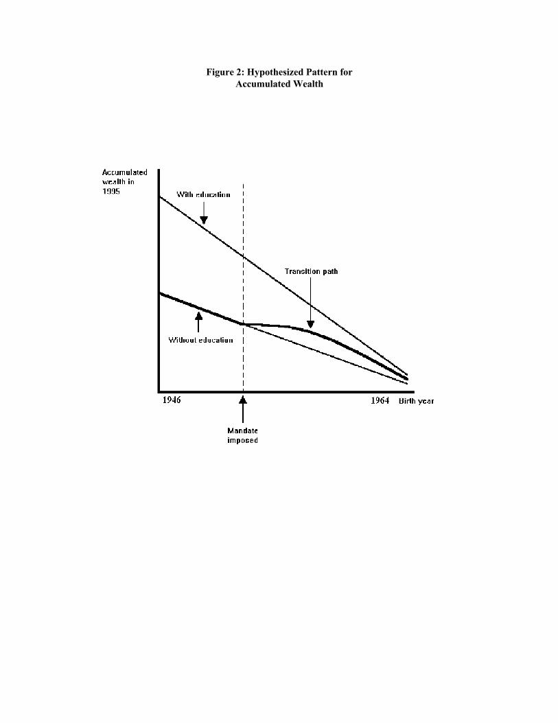
Figure 2: Hypothesized Pattern forAccumulated Wealth

Table 1: Consumer Education Policies by State

State First graduating Consumer education Personal financeclass affected* mandate? mandate?

Alabama 1976 Yes No

Alaska 1964 No No

Arizona 1972 Yes No

Arkansas 1977 Yes (1988) No

California 1975 Yes (1989) No

Colorado No policy

Connecticut No policy

Delaware 1976 Yes Yes

District of Columbia No policy

Florida 1975 Yes Yes

Georgia 1977 Yes Yes

Hawaii 1973 Yes Yes

Idaho 1978 Yes Yes

Illinois 1968 Yes Yes

Indiana 1976 No No

Iowa 1976 Yes No

Kansas 1977 No No

Kentucky** 1975 Yes No

Louisiana 1978 Yes No

Maine No policy

Maryland 1975 No No

Massachusetts No policy

Michigan 1980 No No

Minnesota No policy

Mississippi 1982 Yes No

Missouri No policy

Montana 1972 No No

Nebraska No policy

Nevada 1957 Yes Yes

New Hampshire 1985 Yes No

New Jersey 1976 Yes No

New Mexico 1979 Yes Yes

State First graduating Consumer education Personal financeclass affected* mandate? mandate?

New York 1979 Yes (1986) No

North Carolina 1978 Yes Yes

North Dakota No policy

Ohio 1970 No No

Oklahoma 1978 Yes Yes

Oregon 1973 Yes Yes

Pennsylvania 1978 No No

Rhode Island 1969 Yes (1985) No

South Carolina 1982 Yes Yes

South Dakota No policy

Tennessee 1975 Yes No

Texas 1976 Yes (1979) Yes (1979)

Utah 1978 Yes No

Vermont No policy

Virginia No policy

Washington No policy

West Virginia** 1977 Yes (1983) No

Wisconsin** 1974 Yes Yes

Wyoming No policy

Number with policy: 37 29 14

* If no information on implementation date was available, the first class affected was assumed to be the class graduating in the year after the policy was approved.

** Kentucky withdrew its consumer education policy in 1984, West Virginia withdrew its mandate in 1989, and Wisconsin withdrew its mandate in 1983.

Note: Unless noted, the first class affected by mandate is the same as the first class affected by policy.Source: Alexander (1979), Joint Council on Economic Education (1989), and National Coalition for Consumer Education (1990).

Table 2: General Characteristics of the Sample

Characteristic

Percent married 67.9%Percent female respondent 50.0%Percent homeowner 71.7%Percent African American 6.9%Percent other non-white 12.7%Percent high school degree, no college degree 61.8%Percent college degree 32.3%Average age - respondent 39.6Average age - spouse 40.2Percent took consumer ed. course 42.0%Percent took consumer ed. course with financial topics 29.4%Percent required to take consumer ed. course with financial topics 11.4%

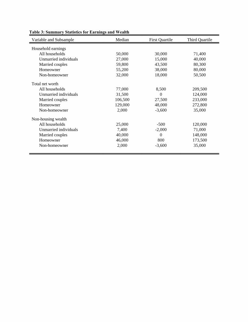
Table 3: Summary Statistics for Earnings and Wealth

Variable and Subsample Median First Quartile Third Quartile

Household earnings All households 50,000 30,000 71,400 Unmarried individuals 27,000 15,000 40,000 Married couples 59,800 43,500 80,300 Homeowner 55,200 38,000 80,000 Non-homeowner 32,000 18,000 50,500

Total net worth All households 77,000 8,500 209,500 Unmarried individuals 31,500 0 124,000 Married couples 106,500 27,500 233,000 Homeowner 129,000 48,000 272,800 Non-homeowner 2,000 -3,600 35,000

Non-housing wealth All households 25,000 -500 120,000 Unmarried individuals 7,400 -2,000 71,000 Married couples 40,000 0 148,000 Homeowner 46,000 800 173,500 Non-homeowner 2,000 -3,600 35,000

Table 4: Exposure to Consumer and Financial Education, Probits

Independent Variable (1) (2) (3) (4) (5) (6) (7) (8)Exposed to Exposed to Exposed to Exposed to Exposed to Exposed to Exposed to Exposed toconsumer consumer financial financial fin. ed., fin. ed., fin. ed., fin. ed.,education education education education required required elective elective

State constants No Yes No Yes No Yes No Yes

State ever imposed mandate -0.0127 0.0403 0.0139 0.0238(0.0263) (0.0312) (0.0214) (0.0262)

Exposed to mandate -0.0567 -0.0605 -0.0227 -0.0277 -0.0326 -0.0506 0.0090 0.0189(0.0562) (0.0620) (0.063) (0.0655) (0.0388) (0.0399) (0.0530) (0.0561)

Years since mandate 0.0271 0.0310 0.0181 0.0240 0.0146 0.0230 0.0007 0.0024(0.0088) (0.0107) (0.0082) (0.0104) (0.0048) (0.0070) (0.0065) (0.0085)

Age -0.0028 -0.0019 -0.0039 -0.0037 -0.0014 -0.0011 -0.0024 -0.0019(0.0024) (0.0026) (0.0021) (0.0023) (0.0015) (0.0016) (0.0018) (0.0019)

Female 0.0889 0.0949 0.0810 0.0867 0.0384 0.0429 0.0405 0.0420(0.0239) (0.0245) (0.0224) (0.0228) (0.0154) (0.0161) (0.0186) (0.0188)

African American 0.146 0.147 0.0857 0.102 0.140 0.132 -0.0544 -0.0339(0.048) (0.051) (0.0456) (0.049) (0.034) (0.037) (0.0366) (0.0395)

Other non-white -0.0133 -0.0042 -0.0213 -0.0107 -0.0040 0.0075 -0.0075 -0.0080(0.0369) (0.0384) (0.0341) (0.0357) (0.0236) (0.0255) (0.0279) (0.0287)

Frugal parents 0.0158 0.0124 0.0212 0.0238 0.0076 0.067 0.0129 0.0157(0.0260) (0.0268) (0.0243) (0.0248) (0.0167) (0.0175) (0.0202) (0.0205)

Percent class attending 0.0157 0.0589 -0.0198 0.0187 0.0076 0.0240 -0.0238 -0.0065 college (0.0497) (0.0524) (0.0468) (0.0490) (0.0318) (0.0341) (0.0391) (0.0406)

Observations 1751 1744 1727 1721 1699 1593 1699 1671

P 44.0 137.1 40.7 127.7 43.3 82.2 11.5 82.52

Coefficients represent probability changes (derivatives for continuous variables, changes for discrete variables). Standard errors are in parentheses.

Table 5: Percentage Rates of Saving

Independent Variable (1) (2) (3) (4) (5) (6) (7) (8) (9) (10)Median Percentile Median Percentile Median Percentile Median Percentile Median Percentile

regression rank, OLS regression rank, OLS regression rank, OLS regression rank, OLS regression rank, OLS

Constant 3.23 40.0 3.66 38.3 3.55 38.1 3.62 39.2 State State(1.87) (4.8) (1.85) (4.8) (1.86) (4.8) (2.00) (4.9) constants constants

State ever imposed -0.520 -1.32 -0.330 -1.51 -0.255 -1.63 -0.314 -0.84 mandate (0.504) (1.59) (0.546) (1.58) (0.601) (1.58) (0.619) (1.74)

Exposed to mandate 0.35 -4.03(1.49) (3.66)

Years since mandate 0.303 0.815 0.299 0.799(0.092) (0.352) (0.104) (0.351)

Years since mandate 0.374 1.30 0.348 1.68 0.352 1.04 * parents not frugal (0.117) (0.44) (0.172) (0.56) (0.190) (0.55)

Years since mandate 0.012 0.100 -0.054 0.428 0.105 -0.110 * frugal parents (0.204) (0.505) (0.255) (0.587) (0.221) (0.589)

Frugal parents 1.69 4.40 1.95 5.11 1.89 5.16 1.30 5.18(0.52) (1.39) (0.57) (1.44) (0.54) (1.44) (0.51) (1.45)

Married 0.435 3.16 0.581 3.09 0.518 3.08 0.575 3.06 -0.073 2.93(0.689) (1.40) (0.688) (1.40) (0.683) (1.40) (0.648) (1.40) (0.597) (1.42)

College educated 1.85 9.30 1.79 8.60 1.88 8.57 1.82 8.55 2.25 8.63(0.52) (1.36) (0.54) (1.38) (0.51) (1.37) (0.52) (1.37) (0.56) (1.40)

Age/10 0.498 0.177 0.307 0.196 0.345 0.198 0.323 0.170 0.622 0.202(0.427) (0.117) (0.458) (0.117) (0.455) (0.117) (0.496) (0.120) (0.450) (0.123)

Total earnings/10 4.00 5.65 3.52 5.52 3.36 5.46 3.43 5.43 3.53 5.195

(0.95) (1.04) (0.93) (1.04) (0.927) (1.04) (1.03) (1.04) (0.97) (1.07)

Observations 1870 1870 1870 1870 1870 1870 1870 1870 1870 1870

Standard errors are in parentheses. For median regressions, standard errors are bootstrapped based on 500 replications.

Table 6: Ratio of Net Worth to Earnings

Independent Variable (1) (2) (3) (4) (5) (6) (7) (8) (9) (10)Median Percentile Median Percentile Median Percentile Median Percentile Median Percentile

regression rank, OLS regression rank, OLS regression rank, OLS regression rank, OLS regression rank, OLS

Constant -2.00 9.96 -1.97 6.28 -2.09 5.76 -1.99 6.08 State State(0.71) (7.22) (0.68) (7.25) (0.69) (7.25) (0.73) (7.25) constants constants

State ever imposed -0.205 -1.29 -0.297 -1.79 -0.316 -1.88 -0.266 -1.86 mandate (0.341) (2.64) (0.316) (2.63) (0.303) (2.62) (0.306) (2.62)

Exposed to mandate 1.02 9.09 1.15 9.00(0.475) (4.05) (0.50) (4.03)

Exposed to mandate 1.26 13.8 1.41 19.7 0.690 9.78 * parents not frugal (0.55) (4.7) (0.87) (6.2) (0.517) (5.16)

Exposed to mandate 0.272 1.51 0.265 7.00 0.135 -1.45 * frugal parents (0.861) (5.63) (0.946) (6.77) (0.723) (5.87)

Years since mandate -0.036 -1.07(0.103) (0.74)

Frugal parents 0.692 7.27 0.781 8.63 0.766 8.60 0.516 7.69(0.266) (2.07) (0.280) (2.19) (0.296) (2.18) (0.264) (2.23)

Married -0.159 -1.99 -0.262 -1.85 -0.125 -1.82 -0.168 -1.79 -0.301 -2.46(0.283) (2.11) (0.276) (2.10) (0.274) (2.10) (0.255) (2.10) (0.257) (2.13)

College educated 0.038 3.13 -0.109 2.12 -0.127 2.30 -0.143 2.45 0.015 2.04(0.218) (2.03) (0.213) (2.04) (0.216) (2.04) (0.213) (2.04) (0.224) (2.10)

Age/10 0.824 9.27 0.814 9.79 0.841 9.83 0.296 9.73 0.775 9.16(0.180) (1.78) (1.65) (1.77) (0.172) (1.77) (0.179) (1.77) (0.161) (1.82)

Total earnings/10 0.771 5.30 0.811 5.07 0.632 4.95 0.857 4.97 0.714 4.765

(0.426) (1.67) (0.442) (1.66) (0.442) (1.66) (0.415) (1.66) (0.414) (1.70)

Observations 911 911 911 911 911 911 911 911 911 911

Standard errors are in parentheses. For median regressions, standard errors are bootstrapped based on 500 replications.