Embed Size (px)
Citation preview

University of South FloridaScholar Commons
Graduate Theses and Dissertations Graduate School
November 2017
Education and Health Impacts of an AffirmativeAction Policy on Minorities in IndiaRobin DhakalUniversity of South Florida, [email protected]
Follow this and additional works at: http://scholarcommons.usf.edu/etd
Part of the Economics Commons
This Dissertation is brought to you for free and open access by the Graduate School at Scholar Commons. It has been accepted for inclusion inGraduate Theses and Dissertations by an authorized administrator of Scholar Commons. For more information, please [email protected].
Scholar Commons CitationDhakal, Robin, "Education and Health Impacts of an Affirmative Action Policy on Minorities in India" (2017). Graduate Theses andDissertations.http://scholarcommons.usf.edu/etd/7017

Education and Health Impacts of an Affirmative Action Policy on Minorities in India
by
Robin Dhakal
A dissertation submitted in partial fulfillment
Of the requirements for the degree of
Doctor of Philosophy
Department of Economics
College of Arts and Sciences
University of South Florida
Co-Major Professor: Kwabena Gyimah-Brempong, Ph.D.
Co-Major Professor: Gabriel Picone, Ph.D.
Giulia La Mattina, Ph.D.
Susan Kask, Ph.D.
Date of Approval:
October 30, 2017
Keywords: quota, caste, gross enrollment ratio, dropout rate, infant mortality, under-five mortality
Copyright © 2017, Robin Dhakal

ACKNOWLEDGMENTS
I would like to thank all of my committee members — Dr. Gyimah-Brempong, Dr. La Mattina,
Dr. Picone, and Dr. Kask — for all of your help and guidance. Without their help, this
dissertation would not have been possible. I would like to specially thank Dr. Kwabena
Gyimah-Brempong for the extra help and support that he has provided to me throughout this
journey. His feedbacks and edits to the paper were invaluable. I would also like to thank Amy
Wagner for spending countless hours to make sure that the grammar in this dissertation is
proper. Similarly, this paper would not have been possible without the help of the Ministry of
Human Resource Development and Ministry of Social Justice and Empowerment of the
Government of India. Finally, a special thanks to Indiastat for putting together all the state-level
data and to the Demographic and Health Survey.

i
TABLE OF CONTENTS
List of Tables…………………………………………………………..………………………………….iii
List of Figures……………………………………………………………………………………………..v
Abstract……………………………………………………………………………………..…………….vi
Chapter One: Introduction……………………………………………………………………………….1
1.1 Background…………………………………………………………………………………..1
1.2 Institutional Setting…………………………………………………………………….……7
1.2.1 Caste System…………………………………………………………………….7
1.2.2 Political Reservation System……………………………………...………….15
Chapter Two: Education…………………………………………………………………………..……19
2.1 Introduction…………………………………………………………………………………19
2.2 Literature Review……………………………………………………………..…………….22
2.3 Data…………………………………………………………………………………………..26
2.3.1 Education data……………………………………………………………………27
2.3.2 Political data………………………………………………………..…………….31
2.3.3 Other variables………………………………………………………….………..32
2.4 Empirical Framework………………………………………………………………………33
2.5 Results…………………………………………………………………………………..……48
2.5.1 Robustness check………………………………………………………….……..52
2.5.1.1 DPD with district level data…………………………………...……..52
2.5.1.2 DPD with state-level election cycle data……………………………53
2.5.1.3 DPD without UTs and newer states…………………………...…….53
2.6 Conclusion and Discussion…………………………………………….………………….54
Chapter Three: Health……………………………………………………………………………….….58
3.1 Introduction……………………………………………………………………………..…..58
3.2 Literature Review………………………………………………………………...…………63
3.3 Data…………………………………………………………………………………………..65
3.3.1 Covariates and determinants of childhood mortality………………….…….67
3.3.1.1 Biological determinants………………………………………………67
3.3.1.2 Socio-economic determinants………………………………………..70
3.3.1.3 Behavioral determinants………………………….………………..…71
3.3.1.4 Environmental determinants…………………………………...……72
3.3.1.5 Political and administrative determinants……………………...…..73

ii
3.4 Empirical Model and Strategy………………………………………………………………….…..76
3.5 Results…………………………………………………………………………….……………..……81
3.6 Conclusion…………………………………………………………….………….…………..………84
Chapter Four: Discussion and Future Research………………………………………….………..…86
References…………………………………………………………………………………...……………90
Appendices………………………………………………………………………………………...……..99
Appendix A: Tables…………………………………………………………………………….99
Appendix B: Figures…………………………………………………………………………..119
Appendix C: Alternative approach: Structural Equation Model…………………………126

iii
LIST OF TABLES
Table 1.01: Literacy rate differentials among social groups in India…………………………..99
Table 1.02: Primary schools enrollment rate differentials among social groups……………..99
Table 1.03: Basic indicator differentials among social groups………………………………100
Table 1.04: Summary Statistics- Education……………………………………………………101
Table 1.05: Pairwise correlation among independent variables……………………….……102
Table 1.06: Fixed effect regression- mediation variables (the mechanism)…………………103
Table 1.07: Dynamic Panel model- SC GER- primary..…………………………………..…….104
Table 1.08: Dynamic Panel model- SC GER- upper primary………………...…….....….…... 105
Table 1.09: Dynamic Panel model- SC GER- secondary…………………………….………....106
Table 1.10: Dynamic Panel model- SC GER- higher secondary……………………………….107
Table 1.11: Dynamic Panel model- SC dropout rates………………………………….….…...108
Table 1.12: Robustness check- DPD with district level data……………………..….…….…..109
Table 1.13: Robustness check- DPD with state-level election cycle data……………..….…..110
Table 1.14: Robustness Check- DPD with data without UTs & newer states………….…….111
Table 1.15: Alternate method- Mediation analyzing using Structural Equation Model
- primary enrollment rates………………………………………...…………..…….132
Table 1.16: Alternate method- Mediation analyzing using Structural Equation Model- upper
primary enrollment rates…………...……………………………………...………...133
Table 2.01: Summary statistics of covariates in the hazard model……………………………112

iv
Table 2.02: Test of proportional hazard assumption- IMR……………...……………………..113
Table 2.03: Test of proportional hazard assumption- U5MR………………………………….113
Table 2.04: Chi-square test of independence of categorical variables…………..………….…114
Table 2.05: Cox Regression for IMR………………………………………………...………..…. 115
Table 2.06: Cox Regression for U5MR………………………………………...…………...…….116
Table 2.07: Cox Regression for IMR – by residence…………………………...………………..117
Table 2.08: Cox Regression for U5MR – by residence…………………………………...…......118

v
LIST OF FIGURES
Figure 1.1: Literacy rate differentials among social groups……………………...……………119
Figure 1.2: Gross enrollment ratio (GER)- primary- by social groups…………………..……119
Figure 1.3: Sample box-plot and regression coefficients- one step GMM…………………....120
Figure 1.4: Sample box-plot and regression coefficients- two step GMM…………………...120
Figure 1.5: SEM path diagram for SC primary enrollment rates………………………….…..130
Figure 1.6: SEM path diagram for SC upper primary enrollment rates……………………...131
Figure 2.1: Data censoring illustration for hazard model- IMR…………………………….…121
Figure 2.2: Data censoring illustration for hazard model- U5MR………………………….…121
Figure 2.3 SC children surviving proportion- by quota quintile……………………………..122
Figure 2.4: Kaplan-Meier hazard plot- IMR………………………………………………….…123
Figure 2.5: Kaplan-Meier hazard plot- U5MR……………………………….…………….……123
Figure 2.6: Kaplan-Meier hazard plot- U5MR by sex- all India……………………....………124
Figure 2.7: Kaplan-Meier hazard plot- U5MR by sex- SC………………………………..……124
Figure 2.8: Kaplan-Meier hazard plot- U5MR by sex- Others…………………………...……125
vi
ABSTRACT
Article 332 of the Constitution of India (1950) stipulates that certain electoral districts in each
state should be reserved for minority groups, namely the “Scheduled Caste”(SC) and the
Scheduled Tribe”(ST), through the reservation of seats in the states' legislative assemblies. Even
though the original article stated that the reservation policy would be in place for just twenty
years, it has been amended several times and is still in effect. This dissertation examines the
impact of the policy on the education and health outcomes of the SC population. Variations in
seat quotas are generated by the timing of elections in different states and the states’ fluctuating
SC populations. The first paper on education uses data from 25 Indian States and 3 Union
Territories for the years 1990-2011 to form a panel dataset to estimate the impact of the quota
system on both enrollment and dropout rates among SC students in all levels of schooling. I use
the fixed effect regression to test the mechanisms through which an elected SC legislator could
have an influence on the education outcomes for the SC population in the represented state. I
then use the resulting variables as my controls to identify the causal relationship using the
dynamic panel data model. I find that a SC legislator has the potential to influence the number
of schools built, as well as the amount of education and welfare expenditure allocated to the SC
population. Moreover, I find that the SC political reservation has a positive and statistically
significant impact on the SC enrollment rates and a negative and significant impact on the
dropout rates, in all levels of schooling. Likewise, I use the NFHS-3 dataset and the Cox

vii
Proportional Hazard Model to estimate the hazard rates (risks of dying) of children under the
age of 12 months (IMR) and under the age of 60 months (U5MR) as influenced by different SC
quota share quintiles. I find that the 50-60% quota-share quintile has the biggest impact in
reducing the IMR and U5MR among the SC children.

1
CHAPTER ONE: INTRODUCTION
1.1 BACKGROUND
Throughout the world, various forms of social segregation create different sects of people
who live as minority groups within national boundaries. A minority population is an often
socially and economically disadvantaged and discriminated group of people. Discrimination is
not only a social and moral issue, but also an economic issue. According to a report1 by the
Center for American Progress in 2012, workplace discrimination causes a loss of $64 billion
every year as a result of reshuffling 2 million American workers due to some form of
discrimination. Similarly, a report2 published by The Atlantic in 2013 concludes that gender
discrimination may have reduced India’s annual growth rate by almost 4% over the past 10
years. Likewise, according to a report3 published by the World Bank in 2014, homophobia and
discrimination cost the Indian economy $30.8 billion every year. The resulting concerns of
economists and others have led to the worldwide development and widespread use of
“Affirmative Action” (AA) policies designed to prevent societal discrimination of historically
disadvantaged groups. Economists have suggested various ways to ensure that those
1 Burns, C. (2012, March). The Costly Business of Discrimination. Center for American Progress. Retrieved from
https://www.americanprogress.org/wp-content/uploads/issues/2012/03/pdf/lgbt_biz_discrimination.pdf 2 Jaishankar, D. (2013, March). The Huge Cost of India’s Discrimination Against Women. The Atlantic. Retrieved
from http://www.theatlantic.com/international/archive/2013/03/the-huge-cost-of-indias-discrimination-against-
women/274115/ 3 Badgett, M.V. L. (2014, February). The Economic Cost of Homophobia & the Exclusion of LGBT People: A Case
Study of India. The World Bank. Retrieved from
https://www.worldbank.org/content/dam/Worldbank/document/SAR/economic-costs homophobia-lgbt-exlusion-
india.pdf.
2
minorities’ rights are protected, not only so that they can become equal and productive
members of societies, but also to ensure that resource allocation in the society is more efficient.
Affirmative action (AA) policies are one of those policies which have been widely used around
the world. Such policies are designed to ensure that the historically disadvantaged groups of
people do not suffer any discrimination in their societies by enacting policies which favor those
who tend to suffer from discrimination. Such policies are often referred to as “positive
discrimination” policies and have been enacted in India to protect some of the social, ethnic and
religious minorities. In this dissertation, I analyze the impact of a particular AA policy, political
reservation, on the education, and health outcomes of a targeted minority group, the Scheduled
Caste (SC), in India.
We can trace the idea of AA in the United States to as early as 1865. However, the term
“affirmative action” was used for the first time in 1961 when Executive Order 10925 was signed
by President John F. Kennedy. The executive order was issued to promote actions that
discourage discrimination by ensuring that government contractors "take affirmative action to
ensure that applicants are employed, and employees are treated fairly during employment,
without regard to their race, creed, color, or national origin." Further executive actions were
taken in 1965, by President Lyndon B. Johnson to discourage discrimination in the hiring
process. Executive Order 11246 required federal and state employers to “take affirmative action
to hire without regard to race, religion and national origin” (gender was added to the list in
1967).
Affirmative action policies in the U.S. have been arguably successful. AA in the U.S. is
mostly applicable to employment and in college admission process. The Supreme Court has

3
been involved a few times in rulings pertaining to affirmative action policies. One of the first
cases was Regents v Bakke (1978) when the Court upheld the AA policy of using race as one of
the factors for college admission. However, the Court also ruled that defining specific quotas is
illegal. Similarly, Grutter v Bollinger (2003) Supreme Court ruling also favored the use of race in
college admission process. Despite some of the successful court cases, affirmative action in the
U.S. remains a contested issue with the Fisher v. Texas (2013) case being the latest related case
discussed in the United States Supreme Court. The general successes of AA in the Court have
resulted in better outcomes for minorities. According to a report published in 2011 by the
Americans for a Fair Chance, there has been an increase in college enrollments of people of
color by 57.2%. Similarly, the proportion of women earning bachelor’s degree has also been
steadily increasing. Likewise, according to statistics from the National Center on Education
Statistics, 65% of African American high school graduates immediately enrolled in college in
2011 compared to just 56% in 2007- that number went from 61% to 63% for Hispanic graduates.
These improvements in enrollments are attributed to the AA policies.
A different form of AA policy had been enacted in India in 1950, 11 years before the U.S
implemented AA to address the rights of African American communities. Even before the 1955
civil rights movement in the United States, India had already implemented a reservation system
(a form of quota-based affirmative action) in its 1950 Constitution, to address the issue of
discrimination against its minority populations. Minorities in India mostly originate from the
social stratification produced by the caste system, which is a key component of Hinduism. Since
over 80% of the Indian population identify as Hindu (Census of India, 2011), the caste system
has resulted in a large minority group. One of these minorities is identified as the “Scheduled

4
Caste” (SC)4 by the Government of India and they form about 17% of the Indian population
(Census of India, 2011). Several articles of the Indian Constitution introduce the non-
discriminatory laws. For example: Article 16(2) of the constitution states that “No citizen shall,
on grounds only of religion, race, caste, sex, descent, place of birth, residence or any of them, be
ineligible for, or discriminated against in respect or, any employment or office under the State.”
Another subsection of Article 16(4) states that “Nothing in this article shall prevent the State
from making any provision for the reservation of appointments or posts in favor of any
backward class of citizens which, in the opinion of the State, is not adequately represented in
the services under the State.” Similarly, Article 46 states that “The State shall promote with
special care the educational and economic interests of the weaker sections of the people, and, in
particular, of the Scheduled Castes (SC) and the Scheduled Tribes (ST), and shall protect them
from social injustice and all forms of exploitation.” The provision for the political
reservation/quota comes from Article 334(a), which states that “Reservation of seats and special
representation to cease after ten years notwithstanding anything in the foregoing provisions of
this Part, the provisions of Constitution relating to the reservation of seats for the Scheduled
Castes and the Scheduled Tribes in the House of the People and in the Legislative Assemblies of
the States.” The reservation of political seats for different minority groups under Article 334(a)
was supposed to expire in 1960. However, the 8th amendment of the Constitution extended the
provision for an additional 10 years. Since then, it has been extended several times by the 23rd,
4 Scheduled Caste does not include all of the “lower caste” population. Brahmnin and Kshatriya are typically
considered to be “higher caste”; Vaisya and Shudra are considered to be “lower caste”. SC designation only applies
to those who are Shudras and who fall outside the caste system, namely Dalits. The caste system is explained in detail
in section 2.2.

5
45th, 62nd, 79th and 95th amendments. The 95th amendment extends the political reservation for
the minority groups until January 26th, 2020.
Even though the quota system in India has been in place for over sixty years, the social
and economic standings of the SC and ST population have not dramatically improved. Over the
past few decades when India saw rising economic growth, the poverty levels among the SC
population continued to grow despite various measures taken by the State and Federal
governments to help the poor population.5 Many studies have pointed out that, over the past
two decades, the SC population has seen a growing incidence of poverty, poor education
outcomes, higher levels of unemployment, higher childhood mortality, and declining rates of
consumption shares (Thorat, 2007; Teltumbde, 1997 & 2001). There have been supporters and
critics of the quota system but the policy has seldom become a national political conversation.
Politicians are unwilling to debate the issue since it would be a controversial political move and
the media and the public are cautious about discussing it, likely because arguing to replace the
system with something else might be seen as being “anti-minority”.
However, the quota system has generated interest among social scientists and
economists over the last decade. The primary question of interest has been “how successful has
this program been?” “Success,” however, has been variably defined by different economists.
Some economists have studied the system’s impact on poverty (Chin & Prakash, 2011; Bardhan,
Mookherjee & Torrado, 2010) and others have looked at the overall transfer of wealth from
higher castes to lower castes in society (Mitra, 2015). Economists have also studied the political
reservation’s impact on policy making (Pande, 2003 and Madhok, 2013). Additionally, some
5 National Council of Educational Research and Training, 2015
6
economists have focused on the system’s impact on crimes and atrocities against minorities
(Prakash, Rockmore & Uppal, 2015). All of these papers conclude that there has been a positive
impact of political reservation on several groups of minorities in India. However, when it comes
to the impact on the Scheduled Caste, there has been varying conclusions. This dissertation tries
to provide more conclusive evidence about the impact of such laws on the Scheduled Caste.
The primary focus of this dissertation is the education, and health outcomes of the SC
group- one of the minority groups that the law targets (ST is the other group). Since the 1950
Constitution of India did not specify a measure of the law’s ‘success’, the true measure of
‘success’ comes from the intent of the law in the first place. The political reservation is
considered to be a constitutional support to those who have suffered discrimination in society
and who lack opportunities in different aspects of the society. In other words, it was put in
place so that the socio-economic status of the lower caste (including the SCs) population in the
society can be alleviated. Various studies6 show that some of the most important issues to
improve the socio-economic status of minorities are education and health, among other areas. In
fact, in his book Development as Freedom, published in 1999, Dr. Amartya Sen highlights the
importance of education and health as indicators and instruments of human development. Sen
argues that development stems from freedom and freedom stems from social opportunities
such as better education access and healthcare. Hence, this dissertation studies the impact of the
reservation laws on two of those important opportunity indicators- education and health. 7
6 Bloom (2007); Sen (1999) 7 The Human Development Index (HDI) also adopts education and health as two of the important measures of
“human development” in calculating its annual HDI index for various countries.

7
The contribution that my research will have relative to existing literature stems from the
specificity of the dependent variables I use. While existing literature has examined the impact of
political reservation on poverty, policy implications, crime, and wealth transfers, it does not
address the impact on the SC population’s education, and health outcomes directly. For
example, Chin & Prakash found that the political reservation for SC did not have any impact on
the SC’s poverty outcomes. However, there is evidence that the SC quotas have increased
transfers from the well-off high caste population to the lower caste population (Pande, 2003).
My dissertation makes a contribution by going a step further in the discussion. I empirically test
if the political quotas for SC have contributed to better education, and health outcomes for this
minority group in India. By providing a definitive assessment of the impact of reservation
policies on the specific socio-economic indicators of the minority, this analysis will fill an
existing gap and be a significant contribution to development economics literature. As the
majority of the SC population falls below the UN’s poverty line, this analysis also has
implications for the effectiveness of poverty reduction policies in India.
The rest of this dissertation is organized as follows: Section 2 of this chapter provides an
institutional background on the caste system and the political reservation system in India.
Chapter 2 discusses the education impacts of the reservation system, outlining the literature
review, data, empirical strategy, and the results. Chapter 3 discusses the health impacts of the
reservation system, outlining the literature review, data, empirical strategy, and the results.
Chapter 4 summarizes the dissertation. The Appendix presents the summary statistic table, the
results table, and an alternative approach taken in this paper

8
1.2 INSTITUTIONAL SETTING
1.2.1 Caste System In India:
One of the large minority groups in India originates from a deep-rooted belief in a
social-stratification system —the caste system. A caste system is a form of social stratification
unique to Hinduism, which groups people hereditarily into distinct occupational divisions.
Most Indian languages use the term "jati" to describe the hereditary social structures known to
us as the caste system. The term “caste” comes from the Portuguese term "casta" — which
means "race". It is commonly believed that Portuguese travelers came to India in the 16th
century and they were exposed to the race-based social stratification system that was already
prevalent in India. Hence, the word “casta” was used — to describe what they saw. The term
has since evolved into "caste" and is widely used to describe social classifications that are
passed along through generations. 8
The origin of the caste system in the region is still debated among scholars. A Hindu
person would explain the origin of the caste system by referring to the Lord Brahma, a four-
handed and four-headed Hindu god, whose hands and heads represent the four castes within
which people are expected to arrange themselves. Indeed, the earliest written evidence of the
caste system comes from an ancient Hindu scripture, Vedas,9 with references to Lord Brahma.
Even though one of the four Vedas, the Rigveda (1500 – 1200 BC), lacks direct reference to the
8 Ushistory.org. (2016). The Caste System. Ancient Civilizations Online Textbook. Retrieved from
http://www.ushistory.org/civ/8b.asp. 9 The Vedas are a collection of hymns and poems written between 1500 and 1000 BC in India. This collection is
considered sacred in the Hindu religion. The Vedas are composed of four different Vedic texts- the Rigveda, the
Samaveda, the Yajurveda and the Atharvaveda. The Rigveda is the largest of these texts, and is considered to be the most
important.

9
caste system and indicates the importance of social mobility, The Bhagvad Gita10 (200 BC – 200
AD) highlights the importance of the caste system in the general society. In addition, the
Manusmriti, a part of The Bhagvad Gita, specifically outlines the rights and duties of the four
castes.
A second set of theory on the origin of the caste system refers to a biological adaptation.
According to this theory, people in India simply specialized to their God-given skills and
attributes– which, over time, transformed the society into a caste system11. However, a more
socio-historical theory links the origin of the castes to the Aryan civilization. The Aryans are
thought to have come to India in about 1500 BC, mostly from south Europe and north Asia. The
theory claims that The Aryans must have introduced the caste system as a means to influence
and control the local population. By the time they arrived, there were other non-Indian groups
already in India, including the Negrito, Mongoloid, Austroloid and Dravidian. In order to
secure their political and economic influence in the society, and to separate themselves from the
“inferior” local population, the Aryans introduced some social and religious rules wherein
specific groups of people would do specific types of work and only the Aryans could be the
priests, warriors and businessmen in society. They were able to maintain and enforce this
structure because of their strong army. This structure paved the way to the more established
caste system that we know today.
10 The Bhagvad Gita, which is written in the ancient language of Sanskrit, is the most revered Hindu scripture. Even
though the origin date of The Bhagvad Gita is still contested, most scholars believe that it was written between the fifth
century and the second century BC. The Bhagvad Gita is not a part of the four Vedas. 11 Ushistory.org. (2016). The Caste System. Ancient Civilizations Online Textbook. Retrieved from
http://www.ushistory.org/civ/8b.asp.

10
A commonly recurring theme in theories about the origin of the caste system, however,
involves the idea of division of labor. The caste system simplifies division of labor by dictating
that people who belong to different castes are responsible for specific and separate jobs. People
would voluntarily assign themselves in doing the jobs that they are good at doing. Over time,
this led to a more formal social stratification system. According to the established system,
people belong to one of four castes: Brahmin; Kshatriya; Vaisya; Shudra. People may also be
born outside of the caste system, in which case they are called Dalits (“untouchables”) and not
permitted to join any caste. As with the castes, the Dalits are not able to climb up the social
ladder. However, they are part of the Scheduled Caste designation. It is important to note that
the caste system only applies to people choosing to follow Hinduism. Brahmins are designated
to serve as priests; Kshatriyas as warriors and nobilities; Vaisyas as farmers, traders and
artisans; and Shudras as tenant farmers and servants. The hierarchy in the social setting is such
that the Brahmins are considered the highest caste and Shudras the lowest caste. Untouchables
are assigned no occupational role in the society.
Although a caste designation originally depended upon the kind of job a person did,
with time, it became a strictly rigid system in which the caste was assigned at birth and passed
down through generations. Each person’s birth assigned caste is unalterable during his/her life
and is also unalterable for his/her children, grandchildren, and so on. Even though the
beginnings of this caste rigidity are hard to trace, it is believed that it is a product of self-interest
on the part of ruling emperors throughout India’s history. However, historical evidence does
confirm that India’s caste system was not originally as absolute and rigid as it has become in
modern times. In fact the Gupta Dynasty, which ruled India from 320 AD to 550 AD, in addition

11
to the Madhuri Nayaks dynasty, who ruled India from 1559 AD-1739 AD, originated from
lower castes. It is important to note, however, that from the 12th century onward, much of India
was ruled by Muslims. During the initial Muslim rule, the Hindu population was marginalized
up to the point where there were hardly any reported populations of Brahmins and Kshatriyas
in northern and central India. The Muslim rule created an anti-Muslim sentiment among the
Indian Hindu population which further strengthened the caste system by inspiring Hindus to
strictly adhere to the elements of their faith, including the caste system. The British took over
India from Muslim rule in 1757 AD, thereby lessening the animosity between the Muslim
Indians and the Hindu Indians. Some of the documented anecdotal evidence reveals that the
British were able to exploit the caste system as a means of social and political control over India.
However, they also identified the underlying discrimination brought upon the lower caste
population (mostly Shudras and Vaisyas), and, responsively created some of the initial anti-
discriminatory laws for the “Scheduled Caste” population of India during 1930-1940.
Typically, the Brahmins and the Kshatriyas are considered “higher caste”, and Shudras
are considered the lowest caste in the hierarchy. However, the official “Scheduled Caste”
designation only includes and protects the Dalits (“untouchables”) who fall outside the caste
system12 which represent about 17% of the national population13. Some of the Shudra
population, who were historically disadvantaged, are officially classified as “Other Backward
Class (OBC)”and also have similar protections in place by the Government of India. This
dissertation strictly focuses on the SC population.
12 Scheduled Caste designation is based on a household’s last name. All of the Dalits fall under this designation. 13 The Scheduled Tribe (ST) does not fall under the “Dalit” designation. The STs are protected because of their
indigenous heritage.

12
Historically, the population of “lower caste” always outnumbered the population of
“higher caste”14. According to the last census taken during the British Empire (1931), the lower
caste represented 54% of the total Indian population. India has never taken a caste-based census
since its independence from Britain. However, according to four different surveys conducted by
the Center for the Study of Developing Societies, between 2004 and 2007, the Brahmins
represented about 5% of the national population and Kshatriyas represented 3.46% of the
national population. Even though the populations of Brahmins and Kshatriyas do not represent
the majority, they constitute a vast number of public officials and politicians in India. According
to the same surveys by the CSDS, Brahmins alone constituted 47% of the chief justices and 40%
of the associate justices in India. Even though the representation of higher caste in the upper
and lower house of the legislative branch of India has been falling— thanks in part to the quota
system— the representation is still disproportionate. Brahmins alone represent about 10% of the
Members of Parliament (MPs) and hold a significant proportion of public offices. The higher
caste population was able to stay in control of governance and form a “majority” in Indian
society because of the better education and increased opportunities that they received by virtue
of their birth-assigned social rank. The extent of the opportunities they received was also
expanded during the British rule, which is why the Brahmins were able to grab a majority of
government positions after India’s independence from the British. Vaisyas, Shudras and Dalits
have comprised a significant portion of the Indian minority in governance for decades. Specific
tribes and some religious groups (Muslim and Christian, in particular) form the other part of
14 The Brahmins and Kshatriyas are generally considered “higher caste”. However, in most of the surveys conducted
only Shudras and Dalits (untouchables) are considered “lower caste”.

13
the Indian population and governance minority. Even though discriminating against anyone
based on caste is illegal in India, peoples’ belief in the ranking inherent to the system is strong.
The fact that people must remain in their birth-assigned castes for life means that
members of the SC population face a significant obstacle in climbing up the economic ladder.
Opportunities for obtaining a higher social status, better education, well-paying jobs, and
political involvement, do not exist for these groups of people. It is for this reason that the Indian
government decided to implement a quota system wherein some seats (and/or positions) are set
aside for people of certain minority classes in employment15, education and in different states’
legislatures. These minority groups are referred to as the “Scheduled Caste” (SC) and the
designation is based on the last names they carry. The Indian Constitution of 1950 lists 1108
different last names under the “Scheduled Caste,” making these people eligible for participation
in the quota system. The tribal minorities are also protected under the quota system and are
referred to as the “Scheduled Tribe” (ST). While the SC classification targets the caste minority
and “untouchables”, the ST classification targets the population who live in tribal areas
(including forest dwellers). There are 744 different tribes listed in this category under the Indian
Constitution of 1950.
The SC population is one of India’s most vulnerable groups despite its growing size.
According to the 2011 national census, the SC population was a little over 201 million, which is
about 17% of India’s total population. Long before the 1950 Constitution of India, this group of
people was considered to be the class of people who did not deserve the rights and protections
granted to the rest of the general population. Because of their position within the caste system,
15 In federal employment, certain percentage of the hiring is assigned for SC, ST or the OBC.

14
the SC population has experienced persistent discrimination and a lack of opportunities in
many socio-economic dimensions. The SC group has been historically deprived of access and
entitlement not only to economic and political rights but also to social needs such as basic
education, health care, and housing. Historical discrimination and exclusion in access to land,
capital, education, and health care have led to high levels of economic deprivation and poverty
among the SCs. The lack of job opportunities has resulted in an SC population with an
exceptionally high dependence on manual wage labor.
Data16 shows that SCs have lower levels of job market skills, higher underemployment,
and lower wage rates compared to rest of the general population because of the limited, if not
excluded, access to capital, land, and education they receive (Saravanakumar & Palanisamy,
2013). According to the National Sample Survey 2011, the average monthly per capita
expenditures (MPCE)17 for SC in rural areas was Rs. 1252 ($18) and in urban areas was Rs. 2028
($29). However, the remainder of India’s population had MPCE of Rs. 1719 ($25) in rural areas
and Rs. 3242 ($47) in urban areas- both values significantly higher than those for the SC’s.
Similarly, the Census of India 2011 shows that only 50.9% of total SC households used some
form of banking services compared to 59.9% of the non-SC households. The census data also
shows that while only 59% of the SC households had access to electricity, 67% of the non-SC
households had access. Likewise, the National Sample Survey 59th round (2003) shows that only
43.3% of SC households owned some land compared to 62.2% of the non-SC households.
16 Data and statistics referred to here come from the following sources: Census of India 2011, The National
Commission for Scheduled Castes (2010), Ministry of Human Resource Development (2011), and the Annual Report
of University Grant Commission 2010. 17 MPCE is the per capita final consumption expenditure of good and services by households.

15
It is important to note, however, that the Scheduled Caste and Scheduled Tribe (Prevention of
Atrocities) Act was enacted in 1989. The Act replaced the caste-based customs relating to
property rights, employment, wage, and education with a more egalitarian legal framework,
under which the SC and the untouchables are granted equal access and rights compared to the
general Indian population. However, despite the legal change, SC’s actual access to land and
other income-earning capital has barely improved. The caste system has continued to function
in the private domain of the economy in modified and changing forms. Empirical studies on
labor, education, housing, and health services have revealed the persistence of market
discrimination towards lower castes, particularly the Dalits (Thorat & Deshpande, 1999; Shah,
Deshpande, Mander, Baviskar & Thorat, 2006). The studies conclude that such discrimination,
despite laws banning it, results in lack of access to capital, more unemployment, and poor
human development, which all together culminate in high poverty and deprivation among the
lower caste population (including the SCs). Some studies also highlight the exclusionary and
discriminatory working of private industrial labor markets (Papola, 2012). It is also important to
note, however, that enforcement of anti-discriminatory laws is often neglected, in part, because
of the deep-rooted belief in the caste system within the law enforcement and the private domain
of the society.
1.2.2 Reservation in State Legislative Assemblies for the Scheduled Caste:
Since this dissertation focuses on the role of political reservation on the well-being of the
SC population, it is important to understand the way seats are reserved and changed for the SC.
It is also critical to understand the role of elected state legislatures in forming policies that affect

16
education, among other sectors. The political reservation in India applies to all states because of
a provision in Article 332 of the Constitution of India (effective January 26, 1950). Specifically,
the article mandates representation of the SC (and the ST) in the State Legislative Assemblies
and the lower house of the Parliament (Lok Sabha.) The numbers of seats reserved for the SC are
to be proportionate to their share of the total population in a state. More specifically, the
proportion of the SC seats in the state assembly is equal to its share of the population as
measured by the latest national census. A “Delimitation Commission” is to be formed after
every national census is conducted. The role of the Commission is to demarcate the
constituency boundaries based on the new population data from the census. Moreover, the
commission revises the number of seats reserved for the SC in each state based on the revised
constituencies and the SC’s new population share. This policy rule allows for some variation in
the SC political reservation. More specifically, the variations come from the following elements:
i) With every new census, the number of reserved seats for the SC changes. The census is
taken every 10 years. After the census is conducted, a Delimitation Commission
is formed. Members of the committee include two Supreme Court and/or high
court judges, the chief election commissioner, and a nominee by the central
government of India. One of the tasks assigned to the committee is to update the
seats quota in the Lok Sabha and the State Legislative assemblies based on the
newly drawn constituency boundaries. In this duty, the committee is simply
matching the reserved seat proportion to the SC population share based on the
newest census. Since the total available seats do not change, the committee has to

17
change the SC quota seats to match the proportion to population proportion.
Thus, the actual number of reserved seats changes every 10 years.18
ii) Since the number of reserved seats can only be a whole number, there is always a
difference between the actual SC population share and the reserved seat share. The small
variation in the quota comes from the discrepancy between the required number
of reserved seats and the number of seats that are actually reserved given that
the number must be an integer.19
iii) When the definition of the SC changes, the share of reserved seats changes. The defining
Constitution of India (1950) listed 1,108 different last names as belonging to the
Scheduled Caste category. However, by 2008, 100 additional last names had been
added to the list. The list has been growing with the last addition approved in
December, 201520. With each added name, the total SC population and hence, its
population share, grows. This, in turn, increases the required seat quota for the
SC.
iv) Year-to-year variation exists because while the SC population size changes every year,
the actual reserved seats do not change as frequently. Since the Delimitation
Commission assigns the reserved seats based on the most recent decennial
18 For example: The 2001 census shows that the SC population in Bihar was 13,048,608 while its total population was
82,998,509. Hence the SC formed 15.72% of Bihar’s population in 2001. Once the Delimitation Commission is formed,
its job is to match the reserved seats proportion to something close to 15.72% of the total available seats. The
Commission finished its job in 2005 when there were 243 seats available in Bihar. Thus, 15.72% of 243 yields 38.20.
The committee established 39 SC-reserved seats 2005 (the policy is to round up to the next higher integer). 19 For example: The ideal number of seats to be reserved in Bihar after the 2001 census was 38.20. However, 39 seats
were chosen to be reserved. Thus, there is a variation of 0.80 in the quota. 20 The addition is mostly due to the demands from several minority groups to be included under SC, so that they can
have political representation and other benefits that the SC gets.
18
census population, but the actual SC population changes yearly (continuously
over any time period), there is year-to-year variation in the SC’s quota share.
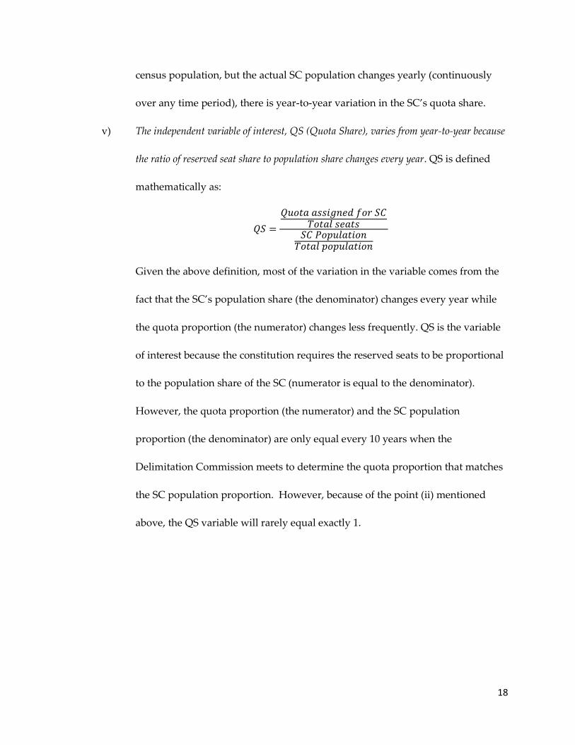
v) The independent variable of interest, QS (Quota Share), varies from year-to-year because
the ratio of reserved seat share to population share changes every year. QS is defined
mathematically as:
𝑄𝑆 =
𝑄𝑢𝑜𝑡𝑎 𝑎𝑠𝑠𝑖𝑔𝑛𝑒𝑑 𝑓𝑜𝑟 𝑆𝐶𝑇𝑜𝑡𝑎𝑙 𝑠𝑒𝑎𝑡𝑠𝑆𝐶 𝑃𝑜𝑝𝑢𝑙𝑎𝑡𝑖𝑜𝑛𝑇𝑜𝑡𝑎𝑙 𝑝𝑜𝑝𝑢𝑙𝑎𝑡𝑖𝑜𝑛
Given the above definition, most of the variation in the variable comes from the
fact that the SC’s population share (the denominator) changes every year while
the quota proportion (the numerator) changes less frequently. QS is the variable
of interest because the constitution requires the reserved seats to be proportional
to the population share of the SC (numerator is equal to the denominator).
However, the quota proportion (the numerator) and the SC population
proportion (the denominator) are only equal every 10 years when the
Delimitation Commission meets to determine the quota proportion that matches
the SC population proportion. However, because of the point (ii) mentioned
above, the QS variable will rarely equal exactly 1.

19
CHAPTER TWO: EDUCATION
2.1 INTRODUCTION
The education system in India consists of nine levels: preschool; play school;
kindergarten; primary school; upper primary (middle) school; secondary school; higher
secondary (pre-university) school; undergraduate; and postgraduate. This paper is concerned
with education in primary, upper primary, secondary, and higher secondary schools. Primary
school (for children aged 6-10 years) comprises grades 1-5; upper primary school (for children
aged 11-14 years) comprises grades 6-8; secondary school (for children aged 15-16) comprises
grades 9-10; and higher secondary school (for children aged 17-18) comprises grades 11-12. In
general, India has seen a rising trend in the literacy rate from just 24% in 1961 to 74% in 2011. A
similar trend is seen for the SC population. In 1961, the literacy rate among the SCs was just
10.3%. The rate has increased to 56.5% according to the 2011 census, thanks to several initiatives
taken by the central and state governments over the past few decades. However, the literacy
rate of the SC population is still significantly lower than that of the remaining Indian population
[Refer to table 1.01].
The increasing trend in literacy rates is primarily driven by the increasing trends in
enrollment rates in various levels of schooling. The increase in enrollment rates, however,
exhibits a similar gap between the general population and the SC population. According to the

20
2001 census, there was a 10% difference between the primary school enrollment rates of the
general population and those of the SC population, which were lower [Refer to table 1.02].
Several factors may explain the low enrollment and literacy rates among the SC
population. One of the biggest factors may be the lack of educational resources and
infrastructure in the rural parts of India. Several papers cite the lack of well-trained teachers,
lack of textbooks, and lack of schools in rural parts of India as the biggest hindrance to the
education outcomes of children in these parts.21 According to the Census of India 2011, 76.5% of
the SC population lives in rural areas, compared to 67% of the non-SC population. Thus, the SCs
are in a position to be most adversely affected by the lack of educational resources in these
areas. In West Bengal, one of the highest SC-populated states in India, 73.3% of the population
lives in rural areas, according to the same 2011 census. Similarly, an increase in the privatization
of schools in several states of India may have created a disincentive for members of the SC caste
to send their children to schools. This is because private schools are generally more expensive
than public schools and the SC population has a lower income level compared to the general
population. The National Sample Survey Round 50th to 68th (years 1993 to 2012) has consistently
shown that an SC person earns about 38.6 % - 40.8% less in a year than a non-SC person in
India. Hence, privatization of schools might lead to fewer enrollments of SC students in costly
private schools since the benefits of education to the SC do not increase at the same rate as the
cost.
Perhaps a more subtle but compelling reason why the SC school enrollment lags behind
general enrollment is the influence of culture and social status on decision making. For instance,
21 Education for rural development: towards new policy responses, 2003; The World Bank; Illiteracy Looms Over
India, The CS Monitor, 1990.

21
the dowry system is still prevalent in many parts of India, especially among the lower caste
population, including the SCs. According to the dowry system, a bride’s family is expected to
give money and furniture to the groom’s family at the time of the wedding. The requested
dowry is always more for an educated girl compared to an uneducated girl. This might provide
a sufficient incentive for SC parents to refrain from sending their daughters to school. In fact,
according to a report published in 2011 by the Ministry of Human Resource Development
(MHRD) of the Government of India, there are 94 female SC students for every 100 male SC
students enrolled in primary and upper-primary school levels. Similarly, the dropout rates for
female students are much higher than those for male students within the SC population and the
dropout rates for SCs overall are higher than those of non-SC caste members22. Additionally,
there have been multiple reports of SC children being targeted for bullying and public
humiliation by higher caste students as well as teachers (Saravanakumar & Palanisamy, 2013).
An expectation of their children being bullied in schools might prevent SC parents from
sending their children to schools; resulting in both lower SC enrollment and literacy rates.
Using state-level data, in this paper I examine the impact of political reservations on the
education outcomes of the SC population. I first use the fixed effect model to establish some of
the mediator variables that the quota system influences. I then make use of these mediator
variables and the variations in the quotas created by the timing of the elections and the
proportion of SC population, to estimate the effect on education outcomes using the dynamic
panel data model (DPD). The DPD model is the best fit for the data because of the
22 According to the Educational Statistics at a Glance report published by the Ministry of Human Resource
Development Government of India in 2011, the primary school dropout rate among SC males was 22.3% and among
SC females were 24.7%. Likewise, the primary school dropout rate for all of India was 22.3% and for the SC
population as a whole was 23.5%.

22
autoregressive nature of the dependent variable, which results in contemporaneous
endogeneity. The DPD controls for this endogeneity problem, which is not corrected by the first
difference or the fixed effect models. I find that India’s political reservation policy has a
statistically significant and positive impact on state-level gross enrollments of SC students in all
levels of schooling. Similarly, I find that the political reservation has a statistically significant
and negative impact on the state-level dropout rates of SC students.
2.2 LITERATURE REVIEW
There are many political economy papers that focus on the impact of affirmative
action policies. Galanter (1984) provides a very thorough qualitative overview of affirmative
action policies affecting SCs, in which he provides a description of different AA policies in the
sectors of employment, education, and politics. Another often-cited work in this field is An
Economic Theory of Democracy (1957), in which Anthony Downs theorizes that candidates who
contest for election for public office are likely to commit to their party’s agendas. Down’s work
is helpful in understanding how a public office candidate from a minority group might have a
bias towards the agenda and policy preferences of the minority group which elects him or her.
The theoretical base for my research is also built upon the work of Osborne and Slivinski (1996).
Their citizen-candidate model concludes that the identity of the candidate running for public
office has an impact on policy determination. This contributes to my understanding that there is
a mechanism through which elected officials are able to influence policy measures, in a way
which may affect the education outcomes of the minorities. For instance, the elected minority
candidate might have an influence on the amount and distribution of a state’s annual education

23
and welfare expenditure, which might have an impact on the well-being of the minorities he or
she represents. According to a report, The Legislature and the budget, published by The World
Bank in 2004, elected legislators in countries including India, Uganda and Zambia, have
significant influence on state’s annual budget allocation. When discussing India, the report
concludes that legislators have direct influence because state budget allocations are decided by
committees of elected legislators. The research endeavor described in this paper attempts to link
existing literature to empirically study the impact of the unique policy of political quotas on the
education outcomes of the SC group.
Several attempts have been made to empirically test the policy outcomes of political
reservation at the small scale level of village council (the Gram Panchayat). Most states have some
seats reserved for the SC, ST, or women for the position of chief of the Gram Panchayats, Pradhan.
Duflo and Chattopadhyay (2004) used the village-level data for the states of Rajasthan and West
Bengal to empirically test the effect of women Pradhans on policy determination. They found
that the Gram Panchayats that elect a female as their Pradhan tend to redirect more public goods
towards sectors that benefit the village, such as access to clean drinking water and paved roads.
Besley, Pande, Rahman, and Rao (2004) conducted similar research on three other states23 to
understand the impact of identity of a politician on the provision of public good. They found
that the Gram Panchayats that elect SC (or ST) as a Pradhan, have a significantly higher
probability of assigning public resources towards toilet, electricity connection and private water
lines. Duflo, Chattopadhyay (2003) also found that a Gram Panchayat with an elected SC
Pradhan directs public resources significantly more to the places where the SC population is
23 The studied states were Karnataka, Tamil Nadu, and Andhra Pradesh.

24
high. More importantly, Bardhan, Mookherjee, and Torrado (2010) found evidence that an SC
Pradhan in a Gram Panchayat in West Bengal secured more benefits from the State and local
governments for public infrastructure improvements such as housing and toilet construction
than did non-SC Pradhan in other Gram Panchayats. These papers provide further empirical
evidence that an elected SC member does have a significant impact on policy determination. I
thus have a solid framework for making an investigation into the direct and indirect influence
of an SC legislator on the socio-economic issues most pressing for the SC, namely education. I
expect to find that the established quota allocation has a positive and significant impact on SC
enrollment rates in all levels of schooling.
In the past decade, various researchers have focused attention on the economic
outcomes produced by political reservation for women. Duflo and Chattopadhyay (2004) found
that, in at least one location in India, the quota reserved for women leaders in public office had
a significant impact on the provision of public goods in the location where the women were
representing. Specifically, the researchers found that the public goods provided were in
accordance to the necessities and priorities of the society. Similarly, Lott and Kenny (1999) have
shown that the gender of the legislators have different priorities in their policy implementation,
while Edlund & Pande (2002) show that male and female tend to have different political stances
on major social issues.
Pande (2003) used the variation in the quota allocation to examine the effects of the
political quota provision in state legislatures on various policy outcomes. Unlike previously
mentioned papers, she used state-level data for 16 of the largest states of India to analyze the
impact of such policies on the transfers to minorities using state and time fixed effects. Pande

25
found that political reservation for SC (and ST) in state legislatures have increased transfers
from higher caste to lower caste population as the law was intended to do. More specifically,
she determined that the SC political reservation has increased the proportion of public jobs
reserved for SC members. Her results confirm the citizen-candidate model previously
discussed, in that they provide specific evidence that a legislator’s identity affects policy
outcomes.
Chin and Prakash (2011) expand on Pande’s (2003) research by examining poverty as an
outcome. If SC legislators have an influence on policy outcomes (as suggested by Pande, 2003),
then, presumably, they have an incentive to prescribe policies that improve the economic
outcomes of the minorities they represent. Working on this theory, Chin and Prakash (2011)
used state level data to study the impact of reservation policies on the overall poverty of a state.
Interestingly, they found that increasing the number of seats reserved for SC has no impact on
the overall poverty of the states. However, they did find that political reservation for ST has
statistically significant impact on poverty reduction wherein a one percentage increase in the ST
seat in the state assemblies would decrease the aggregate poverty level in that state by 1.1% .
Thus, in agreement with Pande (2003), the authors are able to conclude that the identity of
minority legislators can affect key outcomes for represented minorities.
All of the above mentioned studies together show that India’s political reservation schemes
have effects on the policy outcomes and the provision of public goods. Most of the studies also
show that there are some redistribution effects of the reservation in favor of the targeted
minority groups. However, there is no evidence that the reservation is helpful for the SCs in
every sector of their livelihood. In other words, we do not yet know whether the political quota

26
provision will always increase the flow of public resources to minorities in every sector. Hence,
it is imperative to empirically examine whether the reservation system has had an impact on the
basic human development outcomes of the minorities. This paper approaches the question by
estimating the reduced-form effects of the SC political quotas on their education outcomes.
According to the twelfth “five year plan” of the Indian government which spans 2012- 2017,
improvement of education, health, and employment outcomes of citizens are among India’s top
socio-economic priorities. Therefore, it is of interest to know whether the constitutionally
assigned quota system for the SC has been able to improve those outcomes for the SC. While
most of the papers in the literature have focused on understanding the impact of political quota
provision on inputs to the welfare of the SC population such as funding and infrastructure, this
is the first paper to estimate the impact on the outcomes by understanding the causal effects of
India’s affirmative action on the SC’s education outcomes- namely, enrollment and dropout
rates. Previous research, as mentioned above, focuses instead on AA’s impact on policies and
transfers of wealth, which serves as inputs that might have an effect on the outcomes. Although
these investigations brought about a preliminary understanding of the net effect of AA on
minorities, they did not quantify the impact on the SC’s overall well-being. This paper, thus,
fills this crucial void in the existing literature.

27
2.3 DATA
This paper uses annual data from various sources for 25 Indian States and 3 Union
Territories24 for the years 1990-2011. The states of Chhattisgarh, Jharkhand, and Uttarakhand
(previously known as Uttaranchal) were formed in November of 2000 and hence, only enter my
dataset after 2000. The state of Telangana was formed in June of 2014 after it was split from the
state of Andhra Pradesh. For this reason, Telangana is not included in my dataset. The Union
Territories of Dadra & Nagar Haveli, Andaman & Nicobar Islands, Daman & Diu, and
Lakshadweep were not included in the dataset because of a lack of availability of relevant data
and their smaller population size compared to the rest of the states/territories in the dataset. The
state of Punjab has the highest SC population proportion (28%) and the state of Gujrat has the
lowest (7.41%), according to the 2011 census. Both of these states are included in my dataset.
These data form an unbalanced panel because of missing observations for some variables for
some years. For example, my dataset does not have SC enrollment for primary school for the
years 2009 and 2010 due to unavailability of reliable data. Likewise, the SC enrollment data for
secondary and higher secondary level of schooling only spans 2006-2011 in the dataset. While
the quota variable has observations from 1990 to 2013 (with few missing observations for some
states), the GER has large number of missing observations for Arunanchal Pradesh, Assam,
Jammu & Kashmir, Meghalaya, Sikkim, and Tamil Nadu. The state of Jammu & Kashmir has
not kept reliable records of the SC school enrollment because of the armed conflict with
Pakistan since 1947 except for the years 2001-2008. The summary statistics of the variables are
presented in Table 1.04 in the Appendix. Because of the unbalanced panel, the number of
24 Union Territories are the administrative divisions in the Republic of India. These territories are not an established
State of India.

28
observations on table 1.04 is different than the number of observations in the individual
regression tables (tables 1.06- 1.10.) Methods used to deal with unbalanced panel are discussed
in the empirical framework section. All of the included variables are in log form; to avoid the
loss of zeros in some of the variables, I have added one before taking the logs. A description of
the variables used and their sources is provided below.
2.3.1 Education Data
The education outcomes of the scheduled caste group can be measured using various
indicators of education. In this paper, I am particularly interested in the enrollment and drop-
out rates of SC students in primary, upper primary, secondary, and higher secondary levels of
schooling. I use the Gross Enrollment Ratio (GER) for these levels as my dependent variables.
GER is defined as the ratio of the number of students who are enrolled in a school to the
number of children in the population who are of the corresponding school enrollment age. The
United Nations Educational, Scientific and Cultural Organization (UNESCO), officially
describes 'Gross Enrollment Ratio' as the total enrollment within a country "in a specific level of
education, regardless of age, expressed as a percentage of the population in the official age
group corresponding to this level of education." The variables will be referred to as GERP25,
GERUP26, GERS27 and GERHS28 for primary, upper primary, secondary and higher secondary
gross enrollment ratios, respectively.
25 The GERP (Gross Enrollment Ratio- Primary) variable is calculated as SC primary enrollment divided by the
primary-school-going-age population (aged 6-10 in the SC population). 26 The GERUP (Gross Enrollment Ratio- upper primary) variable is calculated as SC upper primary enrollment
divided by the upper-primary school going age population (aged 11-13 in the SC population).

29
Another measure of education outcome which is commonly used in research similar to
my own is net enrollment ratio (NER). In contrast to GER, NER is defined as the ratio of number
of children of official school-going age who are enrolled in school to the total number of
children in the population who are of that age group, expressed as a percentage. Although NER
is an appropriate and respected measure of outcome for education research, I have chosen, in
this paper, to use GER instead of NER for one specific reason. That is, GER includes all
enrollments for each level of schooling regardless of the age of the student, whereas NER
includes enrollments only if the enrolled student corresponds to the defined age group for that
particular level of schooling. As an example of this distinction, consider a case of a 12 year old
student enrolled in primary school, which is technically defined as being for children aged 6-10.
The enrollment of this student is counted in the measure of GER, but not in the measure of
NER. In this paper, I wish to investigate the education outcomes of all SC students, regardless
of whether or not their enrollment corresponds to officially designated age groups. In other
words, for the purposes of this analysis, it does not matter whether an SC student enrolls in
primary school at age 6 or at age 14—what matters is that the SC student is attending school.
Therefore, I have determined that GER is the more appropriate measure of SC education
outcome. Additionally, because the SC are a disadvantaged population, it is reasonable to
suspect that SC children are commonly unable to start school at the officially designated age,
and/or that they experience gaps in education that place them outside of the official age
27 The GERS (Gross Enrollment Ratio- secondary) variable is calculated as SC secondary enrollment divided by the
secondary-school-going-age population (aged 14-15 in the SC population). 28 The GERHS (Gross Enrollment Ratio- higher secondary) variable is calculated as SC higher secondary enrollment
divided by the higher secondary-school-going-age population (aged 16-17 in the SC population).

30
brackets for a grade level. Using GER allows me to measure the education outcomes of these
students rather than pretending they do not exist, as would be the case with NER.
In India, primary education is defined as grades one through five; upper primary
education as grades six through eight; secondary as grades nine and ten, and higher secondary
as grades eleven and twelve. The data for SC enrollment and dropouts were obtained from
Indiastat (indiastat.com), a database that compiles socio-economic data released by various
ministries of India including the Ministry of Human Resource Development of the Government
of India. Some of the enrollment and dropout data that were missing in the indiastat database
were collected using the District Information System for Education (DISE), which is an
education information system operated by the National University of Educational Planning and
Administration (NUEPA). The data cover yearly enrollment and dropout rates for each level
from the year 1990 to 2011.
As noted by UNESCO29 and the World Bank30, one way educational output can be
measured is by assessing access to education. One of the important measures of “access”, as
outlined by UNESCO, is the rate of enrollment in various levels of school. Therefore, GER is one
of the dependent variables I use to study the impact of political reservation on SC’s education.
Likewise, SC children have, historically, been excluded from the formal education system,
which is why various studies have shown that SC children have the highest dropout rates
among any social or minorities groups in India, thereby affecting the gross enrollment ratios
(Saravanakumar & Palanisamy, 2013). Because of this, I have also included dropout rates as
29 Atchoarena, D. & Gasperini, L. (2003). Education for rural development: towards new policy responses. United
Nations Educational, Scientific and Cultural Organization. Retrieved from
http://www.unesco.org/education/efa/know_sharing/flagship_initiatives/towards_new_policy.pdf. 30 Measuring Outputs and Outcomes in IDA Countries (2002), The World Bank

31
my second dependent variable because whether or not the SC children are enrolling in school
and staying in school, offers an indication of whether or not the elected SC legislators are
providing improved access to education for the population they represent.
The education related control variables used in this paper are obtained from Indiastat,
the Census of India, the Ministry of Human Resource Development of the Government of India,
and the Directorate of Economics and Statistics for state governments. Control variables
include: the education budget per SC pupil (EBPP)31, the student-teacher ratio32 (STRP, STRUP,
STRS, and STRHS), the number of schools33 (NoPS, NoUPS, NoSS, and NoHSS), and the adult
literacy rate. Adult literacy rate is included as one of the controls because an educated SC
population should be reflected by an increased rate of enrollment in various levels of schools.
2.3.2 Political Data
Since I am specifically interested in the impact of the political quotas on the well-being
of the SC population, I have used number of SC seats assigned under each state’s legislative
assembly as the variable of interest. State’s Legislative Assembly constitutes of representatives
(Member of Legislative Assembly (MLA)) elected by the voters of electoral districts to the
legislature of a state. Within each state, the seats are assigned at the district-level depending on
the population of SC in each district. The total number of seats assigned for the SC in each state
is determined by the combination of census data and election results. With a few exceptions, the
state elections in India are held every five years. However, not all states have elections during
31 Education budget per pupil (EBPP) is calculated as a state’s annual education budget (in Indian Rupees) divided by
the SC primary to higher secondary-school-going population. The education budget is the amount of a state’s annual
budget that is spent on education. 32 The student-teacher ratio is the number of SC students for every teacher in each State. 33 Number of school variable represents the number of schools which teach various levels of education in each states.
For example NoPS is the number of schools which teach primary level of education.

32
the same year. The variable used in this paper is the SC seat percentage (QS), which has been
previously described in this paper. The SC seats are assigned as a percentage of total legislative
seats available, wherein the proportion is matched to the state’s proportion of the SC
population. These data were extracted from the Election Commission of India’s34 online
database. Detailed election results are recorded by the Commission both for the general
elections and the state elections. The data for SC seat range from 1990 to 2014. It should be noted
that the states formed in 2000 (previously mentioned), only enter the political dataset after their
first elections held in 2002. The ElectionYear variable represents the dummy variable with a
value of 1 if an election was held that year and with 0 otherwise.
2.3.3 Other Variables
Primary and upper primary education were made free in India’s public institutions with the
passage of the Right of Children to Free and Compulsory Education Act of 2009, which went into
effect on April, 2010. In this analysis, I have included the annual per capita income of the SC as
a control variable given that the GER includes enrollment in both public and private schools in
India. As private schools are costly compared to public schools (they were even before the 2009
law), we should expect an SC family’s annual income to have an influence on enrollment rates
in all levels of schooling. The SC annual income per capita35 is calculated based on the Gross
State Domestic Product (GSDP) of each state. Various surveys and studies have shown that over
the past two decades, the average SC annual income is around 40% less than the non-SC annual
34 The Election Commission of India is an independent agency set up and authorized by the Constitution of India to
conduct fair elections. It is also the agency authorized to collect and store data related to federal and state elections. 35 The data on annual per capita income of SC in different states in India is not available in the public domain. Even
the Census of India does not collect this information. Census of India does, however, have data on the different types
of assets that SC households possess at the time of census.

33
income36 (Bhandari, Dutta 2007). Hence, for every dollar that a non-SC person earns, the SC
person earns only sixty cents. The SC annual income variable, is thus calculated as 3*GSDP /
(5*total population – 2*SC population)37.The data for the GSDP of each state is collected from
Indiastat and the Central Statistical Office. Indiastat compiles its GSDP dataset based on
information released by the Ministry of Finance of the Government of India. SC income per
capita is an important control variable because household income is frequently identified as one
of the primary reasons for school dropouts and lack of enrollments (Chauhan, 2016;
Saravanakumar, Palanisamy, 2013). The population data is collected from the Censuses of India
1991, 2001, and 2011. The intercensal population estimates are calculated using the exponential
projection of the population based on the census population data38. The same approach was
taken to estimate the age-group populations of the SC. Within existing literature, exponential
and logistic projections are two of the most-widely used methods for obtaining intercensal
estimates. Additionally, SC population density was calculated by dividing the total SC
population of each state by the total area of the state, as this variable was not otherwise
available. This variable is included to control for the effects of migration of SC population from
one state to the other.
36 The National Sample Survey Round 50th to 68th (1993 – 2012) consistently shows 38.6 %- 40.8% less income for the
SC population. (Source: Ministry of Statistics and Program Implementation, Government of India.
http://mail.mospi.gov.in/index.php/catalog) 37 If A is the per capita income of the non-SC, then the SC’s per capita income is 0.6A. Hence, A*(total population-SC
population) gives the total income share of the non-SC in the GSDP; and 0.6A*SC population gives the total income
share of the SC in the GSDP. These two numbers have to add up to the total GSDP of the states. After some algebra,
we find that the per capita non-SC income is 5*GSDP/(5*total population – 2*SC population), and, 60% of that
number is 3*GSDP/(5*total population – 2*SC population), yielding the per capita SC income. 38 The log-linear function of the exponential population change is given as log(P(t)) = log(P(0)) + t*log(1+r). For
example, the population in 1992 is given by exp(Ln(Pop1991) + (ln(Pop2001/Pop1991)/)2001-1991)* (1992-1991))

34
2.4 EMPIRICAL FRAMEWORK
To estimate the effect of political reservation on the education outcomes of the SC
population, I take advantage of the variations in the explanatory variable (QS) over time and
across states as caused by the above-mentioned factors. Since the quota is assigned according to
the proportion of SC population after every census, the variation caused in QS is exogenous to
the education outcomes of the SC. I assume linear relationships between the SC primary, upper
primary, secondary, and higher secondary gross enrollment ratio (GERP, GERUP, GERS,
GERHS), the explanatory variable of interest, quota share (QS), and the vector of control
variables. The empirical work for this paper is focused on 26 states and 3 union territories of
India for the years 1990-2012. I first test the mechanisms through which the quotas could have
an influence on the GERs using the fixed effect regression. Secondly, I use the dynamic panel
data (DPD) approach to get my estimation because of the fact that there might be some lag
effects of enrollment from one year to the other. As an alternate method of analysis, I also use
the Structural equation model (SEM) to estimate the total effect of the quotas on the gross
enrollment ratios via several mediator variables (see Appendix C.)
Since the panel data is unbalanced, it is important to test for sample selection bias. If the
reason of unbalanced panel is some systemic pattern within states, then the selected sample of
data is not stochastic. Therefore, a bias could be present by the selection of states which is not
randomized which ensures that the selected data sample is not representative of the population.
I have conducted the Heckman Selection Model to test if the dataset has the selection bias. In the
model, rho is the correlation between the errors in the two equations- outcome and selection
equations. Therefore, the null hypothesis rho = 0 means that there is no selectivity bias. For each

35
of the dependent variables, we fail to reject the null hypothesis that the rho is zero. The p-value
for GERP, GERUP, GERS, and GERHS is 0.47, 0.64, 0.48, and 0.97 respectively. This means that
the dataset does not have the sample selection bias. This result is consistent with the expectation
since sample selection bias exists only if the dependent variable is observed exclusively for a
restricted and nonrandom sample from the population. However, we know that both the
enrollment and dropout rates are uniformly observed throughout the sample. Hence, the
sample selection can be assumed exogenous since the unbalanced panel is largely caused by a
lack of data for entire years at a time. More importantly, some of the observations are missing
because of pure lack of availability of reliable data instead of some exogenous unobserved
event. Therefore, even though the unbalanced panel is not ideal, there is no reason to believe
that there is a big loss of efficiency or a significant bias. More importantly, the DPD method
used in this paper can handle unbalanced panel data better than the fixed effects of random
effect methods since the DPD approach does not rely on taking the first difference thereby not
maximizing the gap within the data. Instead, the DPD estimator uses the orthogonal deviations
which preserve the degree of freedom while avoiding the selection bias.
It is also important for me to recognize a mechanism through which the political quotas
might have an impact on the education outcomes of the SC population. It is clear that the intent
of such quota policies is to have a positive effect on the well-being of the minority groups but a
direct link is not as clear. Various studies have theorized an idea of a “role-model” effect,
wherein a representative from a minority group serves as a role model to that group if that
individual is recognized and accomplished in their fields (Fang, Moro 2011; Robb 1999). Duflo
and Chattopadhyay (2004) investigated the importance of the “role-model” effect on the socio-

36
economic status of women. They discovered that in areas with long-serving female Pradhans in
Gram Panchayat, female students tend to set higher goals in their education and hence the
gender gap in various education outcomes has shrunk. Likewise, they also found that SC
parents were 25% more likely to have more ambitious education goals for their daughters,
which in turn helps narrow the gender gap. The authors believe these results stemmed from the
“role-mode effect: Seeing women in charge persuaded parents and teens that women can run
things, and increased their ambitions. Changing perceptions and giving hope can have an
impact on reality.” In the same way, an SC member who becomes an elected state legislator
could be viewed as a role model for other SC members in the state to achieve more and hence,
could drive up enrollment in various levels of schooling. This effect might in fact be larger
among SCs compared to the non-SC population because of the overall fewer opportunities SCs
have to further their socio-economic standing in society. This suggests that the marginal benefit
of education among SCs is most likely higher than that among the non-SCs. Given this reality,
seeing an SC member in a state legislator might persuade SC parents to send their children to
school with a hope that their kids might be able to reach the same level of influence.
Moreover, previous literature (mentioned above) has shown that state legislators have a
significant influence on basic issues such as education in rural India. For instance, elected
legislators have the influential duty of determining state’s annual budgeted expenditures on
education. Education in India is funded by local, state, and central governments. Expenditures
on education from the central government steadily rose from 0.64% of GDP in 1951 to 2.31% in
1970 and peaked at 4.26% in 2000. However, by 2004, education expenditures had dropped to
3.49% of GDP. Similarly, there have been variations among the state’s education expenditures

37
as well. The state’s education budget in West Bengal, for example, was 16.3% of its annual
budget in 2015, which is up by 0.2% from the previous year. It is not unreasonable to expect that
the SC legislators are more likely to fight for more education funding for the SCs than the non-
SC legislators. This hypothesis has been backed by Down’s theory (discussed above), where he
argues that an elected official is more likely to cater to the agenda of the group he/she
represents. Given that elected legislators determine budget, I hypothesize that education
expenditures act as a mediator between the assigned SC quota and the SC enrollment numbers.
Therefore, we expect that education budget will have a positive sign in our analysis.
In addition, each state in India also sets aside a certain proportion of its annual budget
towards “SC/ST/OBC Welfare.” Although the use of these resources depends on the states,
historically, the welfare resources have been allocated towards the betterment of education and
employment of the SC, ST and OBC groups- in addition to urban development and socio
economic justice issues. For example, the Government of West Bengal describes the aim of its
Backward Classes Welfare Department as “to improve the quality of life of these socially and
economically backward classes and enhancement of capability of the people belonging to these
communities, so that they can be very much part & parcel of the mainstream of the Society.”
Several states have created scholarship programs for higher education of SC students using the
welfare funds. Part of the funds is also allocated to fight crimes and atrocities directed towards
those minority groups. This allocation of state resource is in the discretion of the elected state
legislators. . Therefore, I expect that a SC legislator can influence the amount of funding
towards the “SC/ST/OBC Welfare” to a larger extent than a non-SC legislator would. I
hypothesize that the welfare budget acts as another mediator between the assigned SC quota

38
and the SC enrollment rates. Hence, one of the control variables used in my paper is the per
capita welfare budget for the SC (WBPC). WBPC is expected to have a positive impact on the
enrollment of the SC because the welfare budget is intended to expand resources for the SC
population. Similarly, other mechanisms through which an SC legislator can influence SC
enrollment might include the number of schools for primary, upper primary, secondary, and
higher secondary levels and the student-teacher ratios in those levels of schooling.
To test whether a state’s education expenditures, number of schools and welfare
expenditures are influenced by the SC political quotas, I use the following model:
𝑌𝑠𝑡 = 𝛼𝑠 + 𝛽𝑡 + 𝛾𝑄𝑢𝑜𝑡𝑎𝑠𝑡 + 𝑒𝑠𝑡
wherein s=state, t=year, Yst is the state’s education expenditure, number of schools, and welfare
expenditure; Quota is the QS variable described above; 𝛼𝑠 𝑎𝑛𝑑 𝛽𝑡are state and time fixed effects,
while 𝑒𝑠𝑡 is the state level error term. The primary coefficient of interest is 𝛾, which will be the
estimated impact of the quota on the dependent variables mentioned above. The state fixed
effects control for any unobserved time-invariant state characteristics on the dependent
variables while the time fixed effects control for any policies that affect all states uniformly.
Since my omitted variables could be time-invariant or state-invariant, I use the state and time
fixed effect regression to estimate my coefficient of interest. A Haussmann specification test
concludes that the fixed effect method is more appropriate for this dataset than the random
effect model. The results of the model indicate that a state’s education expenditures and the
total number of schools are influenced by the SC quotas. The results of the regression are
discussed on the results section and the tables are in Appendix A. Likewise, to further test those

39
mediator variables, and the causal effects, I have used the Structural Equation Model (SEM),
which was first outlined by Sewall Wright (Wright, 1921). The details of the method and results
are outlined in Appendix C.
The confirmatory evidence about the mediator variable provided can be used to form a
dynamic linear panel model which will estimate a causal effect of the quotas on the enrollment
rates. The functional form can be represented by:
𝒀𝒔𝒕 = 𝜶 + 𝒄𝒔 + 𝜷𝒕 + 𝜸𝑸𝒖𝒐𝒕𝒂𝒔𝒕 + 𝜽𝑿𝒔𝒕 + 𝜺𝒔𝒕 (1)
where, Xst is a vector of variables which includes a state’s expenditures on education per SC
pupil, number of schools for various levels of schooling, election year dummy, overall literacy
rate, SC population density, student-teacher ratio in all levels of schools, the welfare budget
allocated for SC, and the SC income per capita. The education expenditure, welfare expenditure,
and the number of schools are included since these variables represent the infrastructure that is
essential in improving the enrollment in schools, according to a report from Innovations for
Poverty Action (IPA) published in 201239. The election year dummy is included to make sure
that the quota variable does not pick up any election year effects. This allows me to study the
impact of the quota share on the enrollment rates not only for the current year, but also for the
next four years —until the next election is held. The SC population density variable is included
to control for any effect of migration of SC from one state to another between years. Population
density is used as a control instead of the total SC population because the area of some states
has changed over the years within my dataset. The Yst is my education outcome variable in state
39 The IPA report of 2012 also indicates that other factors that improves school enrollment are: improvements in the
labor market, reduction in child labor, reduction in poverty, and reduction in school fees.

40
s and time t. The state fixed effects (cs ) control for any unobserved time-invariant state
characteristics on education outcomes. The Quota variable is the QS as defined earlier. The
primary coefficient of interest is 𝛾, which will be the estimated impact of the quota on the
education outcomes of the minority group. Also, β estimates the time trend and c denotes the
individual state fixed effects.
As with any panel data, there may exist omitted variables that could be fixed for states
over time (time invariant) and that could affect the dependent variable (GERs). This creates the
linear least squares estimates to be bias. If 𝑐𝑜𝑣(𝑄𝑢𝑜𝑡𝑎𝑠𝑡 , 𝛼𝑠)≠ 0, and suggests that the unobserved
variables might be correlated with the independent variables, it would then create an upward
or downward bias depending on the direction of the correlation. It can be expressed as follows.
𝑝𝑙𝑖𝑚 𝛾𝑂𝐿𝑆 = 𝛾 + 𝑐𝑜𝑣(𝑄𝑢𝑜𝑡𝑎𝑠𝑡 , 𝛼𝑠)
𝜎𝑄𝑢𝑜𝑡𝑎2
We can deal with this unobserved heterogeneity by taking the first differences or by
applying the demeaning transformation (fixed effects model). Equation 1 can also be modeled
by the linear least square estimates of the fixed effect model, which are least squares using
deviations from the individual means. Likewise, the first difference estimation can be used
(equation 2) which removes the constant term and the state effects. This equation can be
modelled by the pooled OLS estimator.
𝒚𝒔𝒕 − 𝒚𝒔𝒕−𝟏 = 𝜷 + 𝜸∆𝑸𝒖𝒐𝒕𝒂𝒔𝒕 + 𝜽∆𝑿𝒔𝒕 + ∆𝜺𝒔𝒕 (2)
Both the FE (equation 1) and FD (equation 2) methods explicitly model the impact of Quota on
GER where γ represents the coefficient of the impact. However, for us to estimate the model
using the first difference or the fixed effect approach, strict exogeneity must hold. In other
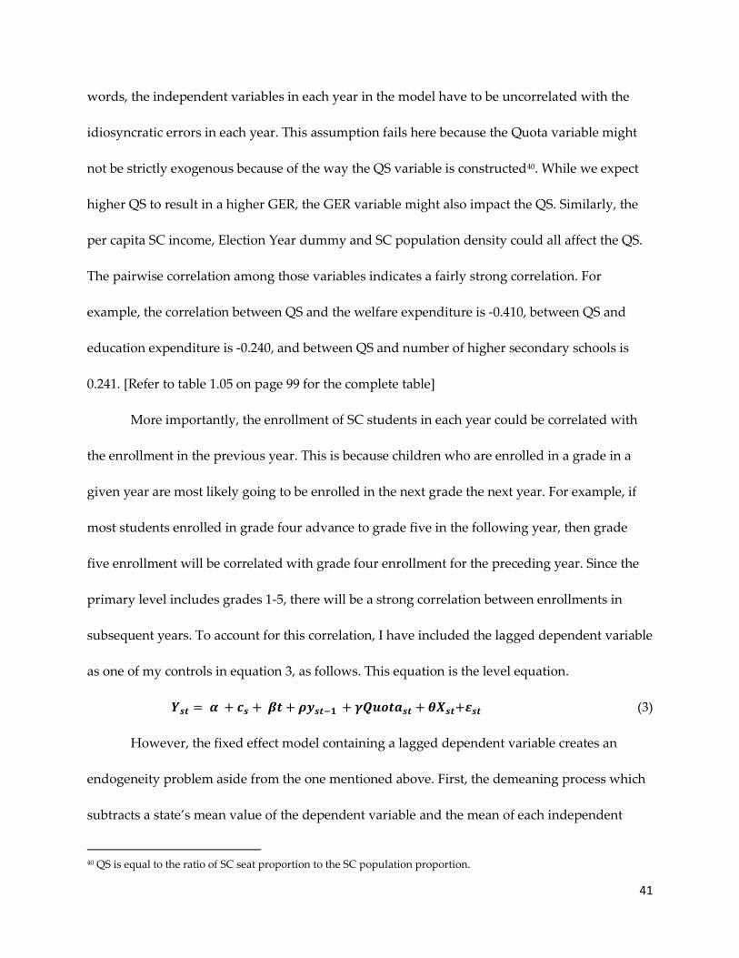
41
words, the independent variables in each year in the model have to be uncorrelated with the
idiosyncratic errors in each year. This assumption fails here because the Quota variable might
not be strictly exogenous because of the way the QS variable is constructed40. While we expect
higher QS to result in a higher GER, the GER variable might also impact the QS. Similarly, the
per capita SC income, Election Year dummy and SC population density could all affect the QS.
The pairwise correlation among those variables indicates a fairly strong correlation. For
example, the correlation between QS and the welfare expenditure is -0.410, between QS and
education expenditure is -0.240, and between QS and number of higher secondary schools is
0.241. [Refer to table 1.05 on page 99 for the complete table]
More importantly, the enrollment of SC students in each year could be correlated with
the enrollment in the previous year. This is because children who are enrolled in a grade in a
given year are most likely going to be enrolled in the next grade the next year. For example, if
most students enrolled in grade four advance to grade five in the following year, then grade
five enrollment will be correlated with grade four enrollment for the preceding year. Since the
primary level includes grades 1-5, there will be a strong correlation between enrollments in
subsequent years. To account for this correlation, I have included the lagged dependent variable
as one of my controls in equation 3, as follows. This equation is the level equation.
𝒀𝒔𝒕 = 𝜶 + 𝒄𝒔 + 𝜷𝒕 + 𝝆𝒚𝒔𝒕−𝟏 + 𝜸𝑸𝒖𝒐𝒕𝒂𝒔𝒕 + 𝜽𝑿𝒔𝒕+𝜺𝒔𝒕 (3)
However, the fixed effect model containing a lagged dependent variable creates an
endogeneity problem aside from the one mentioned above. First, the demeaning process which
subtracts a state’s mean value of the dependent variable and the mean of each independent
40 QS is equal to the ratio of SC seat proportion to the SC population proportion.
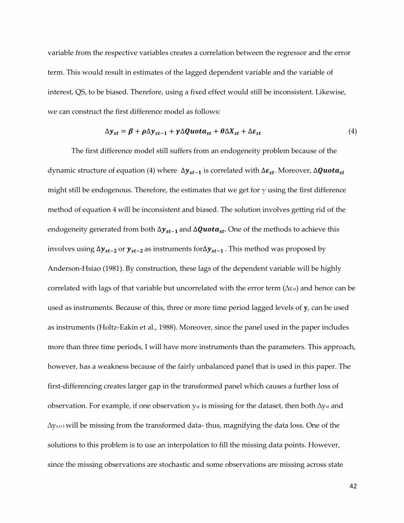
42
variable from the respective variables creates a correlation between the regressor and the error
term. This would result in estimates of the lagged dependent variable and the variable of
interest, QS, to be biased. Therefore, using a fixed effect would still be inconsistent. Likewise,
we can construct the first difference model as follows:
∆𝒚𝒔𝒕 = 𝜷+ 𝝆∆𝒚𝒔𝒕−𝟏 + 𝜸∆𝑸𝒖𝒐𝒕𝒂𝒔𝒕 + 𝜽∆𝑿𝒔𝒕 + ∆𝜺𝒔𝒕 (4)
The first difference model still suffers from an endogeneity problem because of the
dynamic structure of equation (4) where ∆𝒚𝒔𝒕−𝟏 is correlated with ∆𝜺𝒔𝒕. Moreover, ∆𝑸𝒖𝒐𝒕𝒂𝒔𝒕
might still be endogenous. Therefore, the estimates that we get for γ using the first difference
method of equation 4 will be inconsistent and biased. The solution involves getting rid of the
endogeneity generated from both ∆𝒚𝒔𝒕−𝟏 and ∆𝑸𝒖𝒐𝒕𝒂𝒔𝒕. One of the methods to achieve this
involves using ∆𝒚𝒔𝒕−𝟐 or 𝒚𝒔𝒕−𝟐 as instruments for∆𝒚𝒔𝒕−𝟏 . This method was proposed by
Anderson-Hsiao (1981). By construction, these lags of the dependent variable will be highly
correlated with lags of that variable but uncorrelated with the error term (∆εst) and hence can be
used as instruments. Because of this, three or more time period lagged levels of y, can be used
as instruments (Holtz-Eakin et al., 1988). Moreover, since the panel used in the paper includes
more than three time periods, I will have more instruments than the parameters. This approach,
however, has a weakness because of the fairly unbalanced panel that is used in this paper. The
first-differencing creates larger gap in the transformed panel which causes a further loss of
observation. For example, if one observation yst is missing for the dataset, then both ∆yst and
∆ys,t+1 will be missing from the transformed data- thus, magnifying the data loss. One of the
solutions to this problem is to use an interpolation to fill the missing data points. However,
since the missing observations are stochastic and some observations are missing across state

43
and year, the ideal interpolation method is hard to estimate without losing efficiency. More
importantly, since the dataset possess no sample selection bias, interpolation might not be
necessary as long as I have addressed the issue of data loss from the first-difference
transformation. As proposed by Arellano and Bover in 1995, using “forward orthogonal
deviation” instead of the first-differencing of the observations would prevent loss of data from
the differencing transformation. This approach solves the problem of data loss because the
approach subtracts the average of all future observations of a variable from the previous
observations instead of subtracting the contemporaneous value. In each of the DPD regressions,
I have used the orthogonal transformations instead of the first-differences.
However, the instrumental variables approach noted above will likely create
autocorrelation. Moreover, it does not use all of the information available in the data sample.
Arellano and Bond (AB) (1991) proposed an estimator which uses the lags of all predetermined
and strictly exogenous Xs as instruments in addition to the sets of instruments suggested by
Anderson-Hsiao. AB suggests using 𝑌𝑠𝑡−3 as an instrument for 𝑌𝑠𝑡−1. In this paper, I have treated
Quota as one of the predetermined variables because of its construction and used the lags of it
to generate instruments. Arellano and Bond (AB) (1991) used a generalized method of
moment’s approach to construct a valid set of instruments. AB suggests first taking the first-
difference of the data which removes the time-invariant fixed effect (equation 4). Second, use
the lagged dependent variables' values (levels) as instruments for the first-differenced variable,
while making sure that the residuals do not have second-order serial correlation. An issue,
however, is that if the lagged levels are serially correlated, it provides very little information
about the first-differenced variable (Arellano and Bover (1995); Blundell and Bond (BB) (1998)).

44
Therefore, Blundell and Bond (1998) suggested using “system” GMM estimator. In addition to
the first-differencing used by AB, Blundell and Bond use the lagged first differences as
instruments for equations in levels (non-transformed equations.). Hence, the estimation
includes lagged levels as well as lagged difference equations. The two advantages of the system
GMM as opposed to the difference GMM are: 1) it preserves the time-invariant regressors, and
2) it provides a test for autocorrelation in differenced residual terms. The former is particularly
important because states that tend to elect more minorities in state legislatures, likely differ
from other states in ways that affect enrollment and dropout rates as well. For example, if the
SC population is higher in one state, the corresponding QS variable is higher, which might
translate to a higher enrollment of SC students in that state’s schools. Also, the states might be
more progressive which, typically, means more minorities are elected to government, and
resultantly, there may be higher SC enrollment rates in those states. The progressiveness of
states is, in this way, an important factor because SC representatives are capable of running for
and being elected to office even when districts are not SC reserved.
With the Anderson-Hsiao approach, the first row of the instrument matrix corresponds
to t = 2 because the first observation is lost while applying the first difference transformation. If
we include the third lag (𝑦𝑡−3) as a second instrument, we would lose another observation per
panel. To avoid the loss of observation, we can construct the instrument matrix from the second
lag of y as follows where there is one instrument associated with each time period. The
following instrument matrix prevents the loss of degree of freedom because of the inclusion of
zeros and also because it allows all observations t=2 onward to be included in the regression.

45
0 0 …. 0
Ys,1 0 …. 0
0 Ys,2 …. .
Z s = . . … .
. . …. .
0 0 …. Ys, T-2
However, all of the available lags of the original untransformed variables can still be
used as instruments. If we do so, numbers of instruments available for each time period are
different. Hence, as we construct the instruments for higher time periods for each state’s time
series, additional orthogonality conditions are available. Using these additional orthogonality
conditions improves the efficiency of the Arellano-Bond estimator. Similarly, for endogenous
variables, lag 2 or higher can be used. For predetermined variables which might not be strictly
exogenous, lag 1 could be used, as its value is only correlated with errors dated t − 2 or earlier.
The resulting instruments matrix is illustrated below:
0 0 0 0 0 0 … … … …
Ys,1 0 0 0 0 0 … … … …
Zs = 0 Ys,2 Ys,1 0 0 0 … … … …
0 0 0 Ys,3 Ys,2 Ys,1 … … … …
. . . . . . … … … …
. . . . . . … … … …
. . . . . . … … … …

46
However, if all of the available instruments are used, the number of instruments
produced will be large because the number of instruments is proportional to T. Hence, when
constructing the instrument matrix, I have restricted the number of instruments used in the
regression to be closer to the number of groups (n). In all of the regressions, I have selected lags
between five and ten of the dependent variable such that I do not have more instruments than
the number of states. In other words, I use 𝑌𝑠𝑡−5, 𝑌𝑠𝑡−6,…… 𝑌𝑠𝑡−10., of the dependent variable
such that the number of instruments used is linear in T. Choosing a closer lag would likely
create an autocorrelation and hence might have significant AR2 process. If the selected lags are
further out (𝑌𝑠𝑡−11, 𝑌𝑠𝑡−12…), they are less likely to be correlated with the current error term.
However, the correlation between the current and the previous observations might be weaker.
Hence, my selection of the lag depth is justified. I test the validity of the instruments using the
Sargan test and Hansen J test of overidentifying restrictions. As the DPD estimators are the
instrumental variable method, it is important to evaluate the Sargan-Hansen diagnostic tests of
over identifying restrictions. As the system GMM estimator involves a set of additional
restrictions, the Hansens J test for over identifying restrictions is conducted. The regression
statistics and the p-values are included in the results table. The results indicate that the Hansen J
has a p-value of 0.954 which fails to reject the null hypothesis that the instruments are
uncorrelated with the error term (i.e., the instruments are valid), and that the instruments that
were excluded were correctly excluded from the estimated equation (J = 0). Similarly, Table 1.08
shows that the Hansen J has a p-value of 0.568, which fails to reject the null hypothesis of J= 0 as
well. Hence the over identification restrictions in my DPD model are valid. However, in a
model containing large sets of excluded instruments, Hansen J statistics might not be sufficient.

47
This is because the Hansen J statistic evaluates the entire set of overidentifying restrictions.
Hence, Hansen C statistics are also included in the results. The Hansen C test is a mechanism
for testing a subset of the original set of orthogonality conditions. The test statistic is calculated
as the difference between the Sargan statistic for the restricted regression (regression using a
smaller set of restrictions) and the Sargan statistic for the unrestricted regression (regression
using the full set of overidentifying restrictions). Table 1.07 shows that the p-value for Hansen C
is 0.502. Likewise, table 1.08 shows that the p-value is 0.811, which fails to reject the null
hypothesis that the specified orthogonality conditions are satisfied. I have also included the F-
statistics from the first stage in the tables which shows that the instruments used in the
regressions are strong since the p-values are significant at the 1% level.
As pointed out by Arellano and Bover (1995) and Blundell and Bond (1998), the lagged
levels are not the best instruments for first differenced variables. Arellano and Bover proposed
two estimators- one step and two-step estimators and showed that two-step is more efficient.
Hence, I have included the two step system GMM estimator, which avoids the problems of
weak instruments because it uses equations in both the differences (equation 3) and the level
(equation 4). One and two-step GMMs differ in the way their weighting matrices are
constructed. Whereas a one-step estimator is based on an initial weight matrix, a two-step
estimator uses estimates derived from that initial weight matrix to construct a new weight
matrix from which re-estimates of the parameters are obtained. In other words, for the one-step
GMM, one would perform the GMM regression using a weight matrix W = I and get the
estimator, �̂�1. To construct the weight matrix for the two-step GMM, one would obtain the
residuals from the one-step GMM: �̂�𝑡 = 𝑢(𝑥𝑡; �̂�1) and use the residuals to construct a weighing

48
matrix Ω̂�̂�1. Finally, one would then use the new weighing matrix to estimate the GMM
estimator. Hence, the two-step uses the consistent variance co-variance matrix from first step
GMM and is more asymptotically efficient than the one-step estimators. The one step system
GMM estimator is also equivalent to the 2SLS estimator, while the two-step system GMM is
equivalent to the 3SLS estimator because of the use of the consistent variance-covariance matrix
from the first step process.However, in the presence of a large number of instruments, the two
step standard errors can have a downward bias. The bias in the two step standard errors are
corrected by Windmeijer's (2005) finite correction procedure. For this analysis, both one-step
and two-step system GMM are conducted and the results are shown in tables 1.07-1.10.
The DPD is most useful when the data contain large individuals (N) and short time
periods (T). In the paper the panel data is cross-sectionally dominant with 28 individual units
over 21 time periods. If the moment conditions are satisfied, the GMM estimator will be
consistent.
One of the important diagnostic tests in the any dynamic panel estimation is the AR test
of autocorrelation of the residuals. By design, we expect a statistically significant p-value for the
AR1 test because the residuals of the differenced equation should have first order serial
correlation. However, if there are no serial correlation in the original error terms, the
differenced residuals should not have a statistically significant p-value for the AR2 test.
Therefore, for the second lags of the endogenous variables to be a valid of of instruments, we
should have a statistically insignificant AR2 statistic. The p-values for the AR1 and AR2 tests are
included in the results. All of the diagnostic tests validate the DPD approach of estimation for
this dataset.

49
2.5 RESULTS
Table 1.06 shows the results of the fixed effect regressions that were used to verify the
mechanisms through which the political quotas might be able to influence the enrollment rates
of the SCs. In all cases, I use the state and time fixed effects and the reported standard errors are
the robust standard errors clustered on states. Column 1 shows that a 10 % increase in the
previous year’s SC quota share would result in a 1.95% increase in the total number of primary
schools in the current year. Likewise, column 2 shows that a 10% increase in the previous year’s
SC quota share would result in a 3.86% increase in the number of upper-primary schools.
Columns 3 and 4 shows that there is a statistically significant lagged impact of the quotas on the
number of secondary and higher secondary schools. It suggests that a 10% increase in the SC
quota share, two years prior, will increase the number of secondary schools by a 7.3% and the
number of higher secondary schools by a 19.7%. The impact of the 10% increase of quota share
is a 7.82% increase in the state’s education expenditure (column 3) but the state’s welfare
expenditure is not influenced by the political quota (column 4).
Tables 1.07- 1.11 in the appendix show the results of the Blundell and Bond DPD model.
I have used the xtabond2 command developed by Roodman (2009). In all cases, the Arellano
and Bond test of autocorrelation in the first differenced residuals rejects the null hypothesis that
there might be a presence of second-order autocorrelation in the data. Also, all of the reported
estimates show that the Hansen’s statistic for over identifying restrictions is valid. I have
included the AR1, AR2, the Hansen statistic and the Hansen statistics for difference in the
tables. The table also includes the number of instruments and observations. All of the results are

50
derived from the one and two step system GMM method and the stated standard errors are the
robust standard errors.
Table 1.07 shows the estimates of the DPD for SC primary GER. Columns 1 and 2
provide the estimates using the one step system GMM and columns 3 and 4 provide estimates
using the two step system GMM. I find a positive and significant impact of QS on the SC
primary GER. The coefficients on the lagged dependent variable are very close to one, which
suggests the unit root problem in these results. Therefore, I interpret the corresponding beta
estimates with a slight caution. The results from the two-step system GMM (column 3) show
that if none of the proposed mediator variables are used as controls, a 10% increase in QS will
likely produce a 3.84% increase in the gross enrollment rates of SC in primary schools.
However, if the mediator variables are included as controls, column 4 shows that a 10% increase
in QS will likely increase the SC primary gross enrollment rate by 5.55%. This result is
significant at the 1% level. The estimates from the one-step system GMM (columns 1 and 2)
yield a similar result. Column 1 shows that if none of the proposed mediator variables are used
as controls, a 10% increase in QS will likely produce a 3.87% increase in the gross enrollment
rates of SC in primary education. However, if the mediator variables are included as controls,
column 2 shows that a 10% increase in QS will likely increase the SC primary gross enrollment
rate by 3.57%. This result is significant at the 5% level.
The estimates of the DPD for the SC upper primary GER are depicted in table 1.08.
Columns 1 and 2 show the estimates using the one step system GMM and columns 3 and 4
show the estimates using the two step system GMM. I find a positive and significant impact of
QS on the SC upper primary GER. The results from the two-step system GMM (column 3) show

51
that if none of the proposed mediator variables are used as controls, a 10% increase in QS will
likely produce a 3.98% increase in the gross enrollment rates of SC in upper primary schools.
However, if those variables are included as controls, column 4 shows that a 10% increase in QS
will likely increase the SC upper primary gross enrollment rate by 7.64%. This result is
significant at the 10% level. Likewise, column 2 in table 1.08 shows that with all the mediator
variables included, a 10% increase in QS will likely produce a 2.75% increase in gross
enrollment rates of SC in upper primary schools. This result is statistically significant at 10%
level.
Table 1.09 shows the estimates of the DPD for SC secondary GER. Columns 1 and 2
show the estimates using the one step system GMM and column 3 and 4 show the estimates
using the two step system GMM. I find a positive and significant impact of QS on the SC
secondary GER. The results from the two-step system GMM (column 3) indicate that if none of
the proposed mediator variables are used as controls, a 10% increase in QS will likely produce a
12.03% increase in the gross enrollment rates of SC in secondary schools. This result is
significant at the 1% level. However, if the mediator variables are included as controls, the
result is positive but not statistically significant. The estimates from the one-step system GMM
(columns 1 and 2) provide a similar result with a slightly lower magnitude. Column 1 shows
that if none of the proposed mediator variables are used as controls, a 10% increase in QS will
likely produce a 12.18% increase in the gross enrollment rates of SC in secondary education.
However, if the mediator variables are included as controls, column 2 shows that a 10% increase
in QS will likely increase the SC secondary gross enrollment rate by 9.43%. This result is
significant at the 10% level.

52
Table 1.10 shows the estimates of the DPD on SC higher secondary GER. Columns 1 and
2 show the estimates using the one step system GMM and columns 3 and 4 shows the estimates
using the two step system GMM. I find a positive and significant impact of QS on the SC higher
secondary GER. The results from the two-step system GMM (column 3) indicate that if none of
the proposed mediator variables are used as controls, a 10% increase in QS will likely produce a
16.51% increase in the gross enrollment rates of SC in higher secondary schools. This result is
significant at 1% level. However, if the mediator variables are included as controls, a 10%
increase in QS will likely produce a 3.62% increase in the gross enrollment rates of SC in higher
secondary schools (column 4.) The estimates from the one-step system GMM (columns 1 and 2)
provide a similar result. Column 1 shows that if none of the proposed mediator variables are
used as controls, a 10% increase in QS will likely produce a 8.19% increase in the gross
enrollment rates of SC in higher secondary education. However, if the mediator variables are
included as controls, column 2 shows that a 10% increase in QS will likely increase the SC
higher secondary gross enrollment rate by 10.23%. This result is significant at the 10% level.
Finally, table 1.11 in the appendix shows the results for the drop-out rates of SC students
at various levels of schooling. Column 2 shows that a 1% increase in the quota share of SCs
would likely decrease the SC primary level dropout rate by 4.1%. Similarly, the dropout rates
would likely decrease by 5.2% and 1.9% for upper primary and secondary levels of schooling
respectively. These results are all statistically significant at 10% level.
These results show that there is a significant impact of the SC political quotas on the
enrollment of SC children in various levels of schooling. For example, an increase of GER in
primary level of schooling by 5.55% for every 10% increase in QS means that the mean GER

53
increases by 5.87. This translates into an increase in enrollment of SC children in primary school
by 39,448 students. Likewise, the results show that a 10% increase in QS would result in an
increase in enrollment of 20696, 27624, and 28264 of the SC children in upper-primary,
secondary, and higher secondary level of schooling respectively. The sample box-plot and the
corresponding regression coefficients with 95% confidence intervals are given in figure 1.3 and
1.4 in the appendix.
2.5.1 ROBUSTNESS CHECK
I have interpreted the coefficients described in the results as being the result of a causal
relationship between the quota and the enrollment rates of SC students in various levels of
schooling. This interpretation comes from the way that the quota variable (QS) is designed, the
within-state and cross-time variations and the methods used. In this section, I highlight the
three other approaches I have taken to show a similar causal relationship between the quota
variable and the enrollment rates of the SC (i.e. to show robustness). I was unable to perform
these checks for secondary and higher secondary enrollment rates due to limitations in the data.
2.5.1.1 Dynamic Panel Model with district-level data:
It is also important to verify the results using a narrower data set, especially since the SC
quotas are assigned at the district level. Since each state in India is divided into administrative
districts, we can use the DPD model used earlier in the paper with the district level data. Due to
the limitation in the availability of district level data, however, I will not be using any controls
to identify the causal impact. The model identification is identical to the model described in
equation 3 and 4 except that the Xs are not controlled for. The DPD model is more suited for the
district level data because of the large N and small T in this dataset. The results of this model

54
are shown in Table 1.12 in the Appendix. The sign and the magnitude of the coefficient of
interest are as expected to verify the previously obtained core results. Table 1.12 shows that a
10% increase in the QS will likely result in an increase of 1.06% in the SC primary school
enrollment rates. Similarly, a 10% increase in the QS will likely result in an increase of 8.32% in
the SC upper primary school enrollment. The results of this district data DPD model indicate
that my core results are robust and not impacted by the type of data I use.
2.5.1.2 Dynamic Panel Model with state-level election cycle data:
Another robustness check I have performed is to run the same DPD model outlined
earlier, but with the election cycle data instead. For every state, I average the values of each
variable between the election years. If my results truly reflect the causal effect of quotas on
enrollment, I expect to see results similar to my core results by using this dataset instead. To
further test the robustness of the results, I drop the education budget and the welfare budget
variables from this test, as these variables had minimal impact on my core results. By taking the
average of between-elections values for all the variables, I attempt to eliminate the possibility
that election year variabilities are driving the enrollment rates. Hence, I expect to see a smaller
coefficient on my variable of interest (QS) compared to the core results. The Hansen J and C
statistics are all valid and are listed in table 1.13. The results are summarized in the table as well.
The estimates show that a 10% increase in the QS causes the enrollment rates to go up by
12.76% in the primary level and 17.17% in the upper primary level of schooling.
2.5.1.3 Dynamic Panel Model without Union Territories and newer states:
Finally, I check whether my results are driven primarily by the Union Territories and the
newer states that were added to the union. To do this, I only use the state-level data for the

55
states that were created before November, 2000 and exclude all of the Union Territories. I then
use the same DPD method (explained above in the empirical section) to get my coefficient
estimates. The test statistics and the coefficient estimates are given on table 1.14. The estimates
show that a 10% increase in the QS causes the enrollment rates to go up by 27.27% in the
primary level and 22.74% in the upper primary level of schooling. These results show that the
estimates I obtained are robust to the changes of states and union territories.
2.6 CONCLUSION AND DISCUSSION
Although various forms of Affirmative Action policies have been in place in many
countries in the world, the true socio-economic impact of those policies on the targeted
populations has not been definitively assessed. This paper fills the void in the existing literature
by finding conclusive evidence of the impact of one such AA policy in India on India’s minority
SC population. By assessing the impact of India’s political reservation system on its minorities’
education outcomes, I have contributed to the larger discussion on the effectiveness of
affirmative action policies in general. If the goal of the political reservation system in India is to
uplift the socio-economic status of its minorities, and eventually erode away the underlying
social and economic discrimination that still exists based on the caste system, then the
reservation system in India should be considered a “success. “
This paper finds that the reservation system in India has been fairly effective in
improving the education outcomes of the minorities. One of the major findings of this paper is
that the SC quota has a positive and statistically significant impact on the primary, upper
primary, secondary, and higher secondary enrollments of SC students. However, the impact is
highest at the upper primary level. This might be explained by the role-model effect I discussed

56
earlier. If a SC parent sees that a SC member from his/her community has been elected as a State
legislator, he/she is more likely to be encouraged to send their children to a higher level of
schooling. Hence, the effect on upper primary level is higher compared to the primary level of
schooling. We can also notice that the impact on secondary and higher secondary SC
enrollments is not as big as it is for upper primary enrollment. One of the reasons for this might
be the fact that free and compulsory education in India only applies to the primary and upper
primary levels of schooling. Hence, even if the SC parents would be willing to send their
children to higher education, cost of education might be impeding on the enrollment in those
levels.
The gross enrollment ratios (GERs) in various levels of schooling would increase 1.61% -
7.64% for every 10% increase in the quota share of the SC population in a state’s Legislative
Assemblies. Likewise, the dropout rates among the SC students would fall 1.88% - 5.25% for
every 1% increase in the Quota Share. Overall, that’s a very promising indicator that the quota
system is effective in improving the education outcomes of the targeted groups. This means that
in some states, even an increase of one seat for the SC would mean increased school enrollments
and decreased dropouts.
These results are somewhat consistent with those of previous literature. Most of the
previous papers have found little or no effect of SC quotas on poverty or other socio economic
outcomes. However, Chin and Prakash (2011) found that the political reservation for SCs did
not have any impact on poverty reduction of the states but Pande (2003) found that there is
evidence of transfers of resources from high caste to low caste population. My results are
different compared to that of Chin & Prakash since they found no impact of the SC political

57
reservation on poverty in India. However, if we believe that education helps mitigate poverty in
the long run, the findings of my paper is crucial in understanding the long-term effect of
political reservation on poverty. Given that over the past several years the Government of India
has been investing in the education and welfare of SCs, and that Pande (2003) found evidence of
transfer between the castes, I did expect to see a positive and significant impact of SC
reservation on SC education outcomes. Hence, the results of this paper are significant as I have
shown that the SC quota does have a fairly significant impact on the enrollment of SC students
in all levels of schooling. My second contribution to the literature is the establishment of the
mechanisms through which an elected SC legislator via political reservation might have an
impact on the education outcomes of SCs. First, the use of the fixed effect method validates the
mechanisms through which the political set-aside have an impact on the education outcomes of
the SC minority. To further strengthen the argument, I used the SEM mediation analysis (refer
to appendix C), which also shows that an elected SC legislator have a significant influence on
the allocation of state’s resources towards education, welfare, and the number of schools built
annually.
Given the findings of previous studies and this paper, it is clear that political reservation
is not just pro-poor but also pro-minority. If the SC reservation is able to drive up SC enrollment
in schools, it contributes towards India’s twelfth five year plan and it’s Sustainable
Development Goals (SDGs) of achieving universal primary education. A more robust and
aggressive effort from all branches of governments (local, state and central) to complement the
constitutionally granted political reservation, could potentially integrate the SC population into
mainstream India in all socio-economics sectors of life

58
CHAPTER 3: HEALTH
3.1 INTRODUCTION
The health outcomes of people in most of developing countries are still poor compared
to those in developed counties despite the huge amount of received foreign aid, modern
medical advances, and the many NGOs working in the health sector in developing countries.
Two health outcomes that remain especially poor in developing countries are infant mortality
rate (IMR) and under-five mortality rate (U5MR)41. According to the UN World Population
Prospects Report of 2004, 83% (5.3 billion) of the world’s population lives in developing
countries. According to the same UN report, India is home to 21% of the developing world’s
population, and 121 out of every 1000 Indian children will die before the age of 5.42
In many developing countries, minorities usually suffer from socio-economic disparities,
which affect their economic mobility. In India, the Scheduled Caste (SC) population represents
16.6% (206 million) of the total Indian population, thereby forming the largest minority group.
Historically, caste affiliation and social groups have had substantial implications among various
aspects of life in India, including educational outcomes, economic well-being, and career
perspectives. However, with affirmative action and anti-discriminatory laws, access to
resources for SC and other minorities has improved. Nevertheless, studies show that the SC
41 Infant mortality rate is defined as the ratio of number of deaths within the first year of life to every 1000 live births.
Under-five mortality rate is defined as the ratio of number of deaths within the first 5 years of life to every 1000 live
births. 42 Hence, India’s under-five mortality rate is 121..

59
population continues to suffer from economic disparity (Deshpande 2001) which impedes socio-
economic mobility. Various factors including economic well-being, health infrastructures, and
education, contribute to the prevalence of high IMR and U5MR among the people in developing
countries. Moreover, various papers have shown that the IMR and U5MR are significantly
different among various social groups. In particular, research has shown that IMR and U5MR
are especially high among the minorities in the developing countries43. This disparity is noted
by Das, Bhavsar, and Patel (2000) in 1993. They find that in the Indian state of Gujarat, U5MR
varied from 98 among the highest caste’s population to 127 among the lower caste (including
scheduled caste) population. Lower caste, indicative of a minority social group, could thus be
clearly linked to higher U5MR.
Health outcomes, as with many socio-economic outcomes, of India’s SC population,
have been poor compared to the non-SC population. In a caste-dominated country such as
India, SC makes up more than a sixth of the population of India (about 160 million). Even after
the passage of numerous anti-discriminatory laws since 1989, SC population has seen a
continuous violation of its basic human rights for decades. According to a 2007 report by the
United Nations (UN), “[m]ore than 165 million people in India continue to be subject to
discrimination, exploitation and violence simply because of their caste.” The same report goes
on to say that “caste-based divisions continue to dominate in housing, marriage, employment
and general social interaction—divisions that are reinforced through economic boycotts and
physical violence.” It has been documented that these minority groups experience structural
43 Das, N.P., Bhavsar, S. & Patel, R. (2000, November). The growth and development of scheduled caste and
scheduled tribe population in Gujarat and future prospects. International Union for the Scientific Study of
Population

60
discrimination in various forms in the society. Hanchinamani (2001) noted that these groups
experience physical, psychological, emotional, and cultural abuses in their daily lives. These
actions are in-turn legitimized by the society at large.
Various papers and reports have documented that there exists a physical segregation of
living spaces in India, most commonly in the rural areas, forcing poor minority groups44 to live
in some of most unhygienic and inhabitable conditions45. This could affect their access to
healthcare and quality of health service received which impacts their overall health status and
outcomes. According to a report published by the Center for Enquiry into Health and Allied
Themes (CEHAT)46 in 2007, along with poor healthcare access, some groups among the SC
population are especially vulnerable to emotional distress and common diseases. In the
presence of continued structural and social discrimination, obtaining equal access to health
services might be an impossibility. The report also highlights the possibility that the social
views of healthcare professionals in rural areas might impede access to healthcare for the SC
population. The doctor’s attitudes towards the social structure of the caste system might also act
as a barrier for the SC to receiving quality healthcare from the already available healthcare
system if SC members suspect they will face discrimination.
Although data and studies on the nature of discrimination faced by SC in the health
sector are very limited, there is indirect evidence of discrimination reflected in some of the
health indicators among the SC population. Some of the most pressing health concerns for the
44 The mentioned reports suggests that these rural dwellers are mostly Scheduled Caste population and religious
minorities. 45 Minorityrights.org; Development of Scheduled Castes and Scheduled Tribes in India, 2008; National Campaign on
Dalit Human Rights (NCDHR) 2008. 46 Chatterjee, C., & Sheoran, G. (2007). Vulnerable groups in India The Centre for Enquiry into Health and Allied
Themes (CEHAT), 1-21.

61
SC are various measures of child mortality. According to the NFHS-3 survey conducted in 2005-
2006, 66 out of 1000 SC babies die before their first birthday, compared to 57 out of 1000 babies
among the all population of India. Similarly, for every 1000 new births, 88 SC children died
before their fifth birthday compared to 74 for all population of India. Likewise, other indicators,
including NMR47, PMR48 and CMR49 are significantly higher for the SC children compared to the
all India population. Table below, depicts statistically significant SC versus ST and all India
comparison of the various indicators related to children mortality based on the NFHS-3 2005-
2006 surveys.
Social
Group
Neo-natal
mortality
(NMR)
Perinatal
mortality
(PMR)
Infant
mortality
(IMR)
Childhood
mortality
(CMR)
Under 5
mortality
(U5MR)
Childhood
vaccination
(full
immunization)
(%)
SC 46.3 55.0 66.4 23.2 88.1 39.7
ST 39.9 40.6 62.1 35.8 95.7 31.3
All India 39.0 48.5 57.0 18.4 74.3 43.5
However, it is also important to understand that the health outcomes are dependent on
the type and extent of health infrastructures available to the SC population. Although it is
difficult to quantify the number of health centers or doctors working exclusively for the SC
population, examining the health infrastructure in the rural areas of India, where 80% of SC
live, provides an indication of the resources available to them. According to the RCSH survey of
47 Neo-natal mortality rate (NMR) is the number of deaths among the children less than 28 days old, out of every 1000
live births. 48 Perinatal mortality rate (also referred to as Pre neonatal mortality rate) is the number of fetal deaths (stillbirth), out
of every 1000 live births. 49 Childhood mortality rate (CMR) is the number of deaths among children aged 1-4, out of every 1000 live births.

62
2004, only 68.3% of the rural villages in India had at least one Primary Health Center (PHC).
Similarly, about 79% of the villages had a government hospital. According to the same survey,
close to a hundred percent of urban areas have PHCs and government hospitals. However,
many of those facilities in rural areas are not accessible throughout the year because of poor
road conditions- a third of the villages are affected. According to a different survey (NSSO
2004), the total medical expenditure per treated patient in rural India was INRs. 257 while that
in urban India was INRs. 306. Of that amount, people in rural India spent just INRs. 26 per
capita in private medical facilities, compared to INRs. 299 in urban India. These figures indicate
that minorities living in rural India have much less infrastructure to help them improve their
health outcomes.
The goal of this paper is to assess, through an indirect effect, the impact of the political
reservation on the IMR and U5MR of the SC population. Since some of the previous literature
has shown that a minority representation in local, state, and federal branches of governments
have influence in policy matters, we should expect similar influence in the health sector.
Increased representation of a specific minority caste in an executive function in a governmental
sector might improve the provision of public goods and health infrastructures for members of
that caste. Some of the ways that a minority representative might have an impact on the IMR
and the U5MR of its people is through local and state health expenditures, the number of PMCs
and governmental health facilities and other health infrastructures. Additionally, a direct effect
may be present, for example in the case of a “role model” effect, wherein the successful election
of an SC member inspires SC parents to imagine greater potential for their children and invest
in them accordingly. Hence, both indirectly and directly, an SC representative has the potential

63
to positively influence the IMR and U5MR for the SC population. I study the impact of such
representation on IMR and U5MR based on the DHS health survey of 2005-2006 using the Cox
Proportional Hazard Model.
3.2 LITERATURE REVIEW
Many papers have highlighted the determinants of childhood mortality in developing
countries. However, very few have studied the impact of affirmative action policies on
childhood mortality. Van Den Berg, Bergemann, and Sumedha (2010) created a proportional
hazard model using data from the National Family Health Survey (NFHS 3) to identify the
impact of employment quotas in India on the childhood mortality rates. The employment
quotas in India went into effect in 1950 for the SC and ST population and in 1993 for the OBC
population, reserving a sizable portion (just under 50%) of the public sector jobs for these castes.
The authors control for various biological, environmental, and socio-economic factors, as well as
for some of the macroeconomic indicators of specific Indian states. They find that the
employment quotas are able to decrease childhood mortality among the SC children. They also
find that this decrease is substantially greater in India’s rural areas as opposed to its urban
areas. This paper conducts an analysis similar to Van Den Berg, Bergemann, and Sumedha
(2010), except examining the effect of the political reservation instead of the employment
quotas. As was the case with employment quotas, I expect political quotas to have a negative
and significant impact on the mortality of SC children.
The determinants of childhood mortality have been debated in the medical science field
as well as in the social science sector. However, there is a consensus on some of the biological,
environmental, and socio-economic factors that can drive mortality in children. Sonia Bhalotra

64
has published several papers studying the impact of birth spacing (Bhalotra and van Soest,
2007), economic growth (Bhalotra, 2008), state health expenditure (Bhalotra, 2007) and religion
(Bhalotra, Valente, & van Soest, 2008) on childhood mortality. In all cases, Bhalotra and her co-
authors use a dynamic panel data model to study the impact of these determinants, ultimately
concluding that longer birth spacing, economic growth, and higher state health expenditure
each reduce childhood mortality. They also find that religion plays a role, wherein a Muslim
child in India faces a higher risk of childhood mortality than a Hindu child.
Masset and White (2003) also examined several determinants of mortality in children.
Restricting their analysis to the Indian state of Andhra Pradesh, they used a Cox proportional
hazard model to identify specific determinants of childhood mortality. They then compared the
hazard ratios and the coefficients to those of the state of Kerela. Their analysis indicated that
key determinants, including birth spacing, a mother’s health, and environmental factors, act as
driving causes of childhood mortality. As discussed by Grossman (1972) in his book The
Demand for Health: a theoretical and empirical investigation, a household’s income drives its
demand for healthcare. However, health has negative income elasticity. Grossman’s
explanation for this is that “the income elasticities of the detrimental inputs in the health
production function exceed those of the beneficial inputs”. In order to test the income as one of
the determinants of childhood mortality, I use the “wealth index” as proposed by the
Demographic and Health Surveys (DHS), and as a necessity, because DHS does not collect data
on household income.
The mechanism through which an elected minority representative might have an impact
on childhood mortality is important to identify in this analysis. As highlighted in section 2.2 on

65
chapter two, the established mechanism is the type of policy and budget influence that an
elected official might have. For example, Downs (1957) concluded that an elected official might
have a bias towards the agenda of the group he/she represents. Likewise, Osborne and
Slivinski’s (1996) Citizen-Candidate model revealed that the identity of the candidate running
for public office has an impact on policy determination. This contributes to my understanding
that a minority legislator could influence certain policy measures affecting the associated
minority population, and that these measures, in turn, could have implications for that
population’s health outcomes. As an example, the elected minority candidate could be involved
in determining the amount of a state’s annual health and welfare budget, allocated to the
represented minorities, potentially improving the well-being of those minorities. Pande (2003),
Duflo and Chattopadhyay (2004), and Chin and Prakash (2011) have studied the various
possible mechanisms and the impact of the political reservation laws on various measures of
well-being of the targeted minority groups. Assuming that the elected SC representatives care
for the policy preferences of the group he/she is representing, or they care about their re-
election prospects, I hypothesize that such policy preferences will improve the health outcomes
(namely, IMR and U5MR) of the represented group.
3.3 DATA
The health data used in this paper comes from the National Family Health Surveys
(NFHS 3) of 2005. The dependent variables of interest are infant mortality rate (IMR) and under-
five mortality rate (U5MR), as measured by the probability of SC children dying within 1 year
and 5 years respectively. Outside of the NFHS surveys, data on mortality rates among the SC

66
population for various states are difficult to find. Although the IMR and U5MR can be
estimated from data from the Sample Registration System (SRS) and demographic surveillance
systems, these systems are not widely used in developing countries. India, does in fact, release
data from a SRS system, however, these data are considered to be less comprehensive, and less
reliable, and are of uncertain accuracy. Additionally, the SRS system does not record all socio-
economic information, making an analysis of the socioeconomic inequalities in mortality
impossible. Furthermore, information specific to the SC population and their health service
provided is inadequate and inconsistent, within the SRS system, because of missing data on
many crucial variables. Therefore, the best source of data on childhood mortality for this
analysis is a household survey such as the NFHS.
The NFHS-3 dataset provides information on birth and death histories of the
respondents and their children. To estimate child mortality rates from NFHS dataset, we can
use the fertility histories of the women respondents in the survey. These can be constructed
based on responses to questions asked to women of child-bearing age about births and deaths
of their children. The comprehensiveness of the NFHS data allows for a compilation of child-
level data containing information for each child on the date of the mother’s interview;
specifically: the date of birth of the child, a binary variable indicating the child’s status (alive or
dead), and the survival time. Mortality estimation is based on deaths over a specific period of
time—usually the 5 or 10 years before the survey date. The NFHS-3 dataset includes birth
histories of 124,385 women (aged 15-49) out of which about 23,125 women were from the SC
group. The summary statistics of all variables are listed in table 2.01 in the appendix. Each of
those variables are discusses in detail in the next section.

67
I have also incorporated health infrastructure data into the analysis. The data on number
of primary health centers and the number of doctors comes from the Ministry of Health and
Family Welfare, which spans the period 1970 to 2005. I have also included the health
expenditures by states as one of the controls. These data were collected from indiastat.com and
from states’ annual budget reports. The socio-economic covariates in the paper are derived from
the NFHS surveys. I have used place of residence, age of mother, and medical attention for
pregnancy and delivery as the socio-economic determinants of infant and under five mortality
rates. I also control for the household’s annual income. The following section describes the
covariates used in the empirical analysis in more detail.
3.3.1 Covariates and Determinants of Childhood Mortality
The determinants of childhood mortality used in this paper are based on the findings
reported in previous literature. The determinants can be consolidated into four different groups
— biological, socio-economic, behavioral, and environmental variables — which are described
further below and are used in the model described in the next section.
3.3.1.1 Biological Determinants:
The biological determinants of childhood mortality used in this paper are: birth order of
the children, mother’s age at birth of the child, length of birth intervals, and gender of the child.
Although the relationship between birth order of a child and mortality is not conclusive, several
health scholars expect mortality to be higher for a woman’s first child. Sullivan (1994) noted that
higher mortality among first born children in developing countries can be attributed to the fact
that women in rural parts of developing countries may have their first child before they have

68
reached reproductive maturity. Additionally, a paper published by the World Health
Organization (WHO) in 200050 shows that the IMR of first child in India is 93, while that of
second and third child is 77 and 72 respectively. Likewise, U5MR among the first child is 117,
while that for second and third child is 106 and 107 respectively51. In the dataset, 32.95% of the
children reported were the first child to the mother. Among the SC respondents, 30.81% of the
reported children were the first-born.
According to the same WHO report, IMR and U5MR are much higher among children
born to adolescent mothers (aged 10-19) and to older mothers (aged 35 and up). Pebley and
Strupp (1987) concluded that the higher mortality rates among children born to adolescent
mothers might be due to the fact that these women have not yet reached reproductive maturity.
Similarly, the higher mortality rates among children born to older mothers may be a result of
natural age-based deterioration of these women’s reproductive health. According to the NFHS3
survey, 27% of surveyed women gave birth to a child before they turned 20. IMR among
children born to mothers less than 20 years of age is 107 and among the children born to
mothers age 40-49 is 112. Likewise, the U5MR is 141 for adolescent mothers and 163 for older
mothers. All other mother age-groups have significantly less IMR and U5MR. Given that the
relationship between mother’s age and childhood mortality is U-shaped, wherein childhood
mortality is highest at lower age groups and at higher age groups, I use the mother’s age and
mother’s age squared as controls. In the survey sample that is used in this paper, the mean age
of the mother (SC and otherwise) was 23 years.
50 Claeson, M., Bos, E., Mawji, T. & Pathmanathan, I. (2000). Reducing child mortality in India in the new millennium.
Bulletin of the World Health Organization, 78(10), 1192-1199. 51 All of the IMR and U5MR numbers are expressed as the number of deaths out of 1000 new births.

69
One of the most important biological determinants of childhood mortality is the interval
between births. Arulampalam & Bhalotra (2004) find that if a child is born in a household after
the death of a previous child, the probability of the child dying as a newborn increases. The
United Nations International Children’s Emergency Fund (UNICEF) determined in a 1999
report on developing countries that “a child born within 24 months of the previous child has a
68% higher risk of dying within the neonatal period and a 99% higher risk of dying in the post-
neonatal period.” Furthermore, the risk significantly increases if the previous child had died.
The 2000 WHO report also shows that the IMR among children born within 24 months of the
previous birth is 130 and the U5MR is 178. These rates become significantly smaller if the birth
interval increases to more than 48 months (IMR of 42 and U5MR of 57). Boerma and Bicego
(1993) analyzed the relationship between birth interval and mortality and concluded that the
reason the mortality rate is high if the birth interval is low, is that the mother’s body is not fully
recovered from physical and nutritional depletion if the interval between births is less than 24
months. In the survey sample that is used in this paper, the average birth interval among SC
mothers is 32 months. Finally, gender of the child is also an important determinant of childhood
mortality. There is a general consensus that male children have a higher mortality probability at
all ages of childhood because of genetically determined characteristics. However, in many
developing countries, including India, the existence of a cultural preference for a male child
over a female, causes me to expect that the IMR and U5MR for female will be higher. Sullivan
(1994) and Croll (2001) both noted this relationship. In the sample, 48.04% of the SC respondents
were female.

70
3.3.1.2 Socio-economic Determinants:
The socio-economic determinants of childhood mortality used in this paper are: the
mother’s highest education level and her household’s economic well-being. The relationship
between a mother’s education and her child’s probability of dying is well documented52. As
Sullivan (1994) discovered, children of illiterate mothers have a higher probability of dying at
all ages than those of educated mothers. This may be attributed to the fact that, compared to a
poorly educated mother, a well-educated mother is likely equipped with a better understanding
of relevant environmental threats and the appropriate usage of healthcare methods and
facilities. The WHO report (2000) on India supports this finding, indicating that if a mother is
illiterate, her children’s average IMR and U5MR are 101 and 141 respectively. These mortality
rates drop significantly if the mother has a high school or higher education; in this scenario,
IMR and U5MR are 37 and 43 respectively. In my dataset, 64% of the SC women did not have
any formal education.
Since the NFHS survey data do not contain information on the respondent’s income, I
use the wealth index calculated based on the ownership of different asset types as a measure of
“economic well-being”, as recommended by DHS. According to DHS guidelines, a Principal
Components Analysis (PCA) is first conducted and the coefficient recorded for each of the
assets. Second, the PCA coefficient, mean and the standard deviation for each asset are used to
find a wealth index associated with possession of each asset. Finally, the individual scores are
added to obtain the wealth index of the households. I then use DHS’s guideline to divide those
wealth indices into five quintiles — poorest, poorer, middle, richer, and richest for each of the
52 Retherford (1989), Palloni & Tienda (1986), Pebley & Strupp (1987), Shiva Kumar (1995), Boerma & Bicego (1993),
Bourne & Walker (1991)

71
households. I expect the “poorest” quintile to have the higher childhood mortality rates and
“richest” quintile to have the lowest childhood mortality rates. In the sample, 22% of the SC
respondents were classified as “poorest”, 22% were “poorer”, 20% were “richer”, and 14% were
“richest”.
3.3.1.3 Behavioral Determinants:
The behavioral determinants of childhood mortality used in this paper are: tetanus
immunization, the number of antenatal visits, mother’s knowledge of oral rehydration salts
(ORS), and the total absence of breast feeding. According to the UNICEF report published in
1999, 73% of U5 mortality in India is a result of low-cost treatable diseases. Among them,
diarrhea, respiratory diseases, tetanus, and measles account for 60% of all deaths of children
under-five years of age. In my dataset, only 11% of the SC respondents had used tetanus
immunization on their children. The report also notes that 60% of childhood mortality would be
preventable by the use of antibiotics, immunization, and oral rehydration methods (ORS).
Gupta (1990) found that immunization and mother’s knowledge of ORS are two of the key
behavioral determinants of IMR and U5MR. Similarly, many scholars have noted that antenatal
care is very important in the early health of a child53. Hence, I use number of antenatal visits and
the mother’s knowledge of ORS as two of the controls in my regression. Only 1.5% of the SC
respondents in the dataset had used ORS and 11% had used some antenatal care. Additionally, I
53 Acharya, L., & Cleland, J. (2000). Maternal and child health services in rural Nepal: does access or quality matter
more?. Health Policy Plan, 15(2), 223–229.
Addisse, M. (2003, January). Maternal and Child Health Care. University of Gondar. Retrieved from
https://www.cartercenter.org/resources/pdfs/health/ephti/library/lecture_notes/
health_science_students/ln_maternal_care_final.pdf.

72
have chosen to incorporate a dummy variable of whether or not the child was breastfed as a
behavioral determinant of childhood mortality. There is a consensus in the medical science
literature that as a mother’s milk is highly nutritious and rich, it can prevent many illnesses and
diseases for a breastfed child. Palloni & Tienda (1986) found empirical evidence that a breastfed
child has a lower probability of dying compared to a non-breastfed child. Hence, I expect to find
in this analysis that a breastfed child has a lower probability of dying. In the dataset used, 75%
of the SC women did not breastfed their child.
3.3.1.4 Environmental Determinants:
The environmental determinants of childhood mortality used in this paper are: absence
of a toilet, absence of an accessible and safe source of potable water, and use of unsafe
(potentially toxic) fuel sources such as dung, wood, and coal for cooking. As Mosley and Chen
(1984) noted in their framework for the study of childhood survival in developing countries,
medical science has reached an overwhelming consensus that the environment a child is born
into has an enormous impact on the child’s probability of dying. A report published by the
International Institute for Population Sciences (IIPS) in 2000 observed that diarrhea and acute
respiratory infections are two of the major causes of mortality among children under five years
of age in India. Water and air quality are known to be major contributors to diarrhea and
respiratory infections. In a fact sheet report published in 2006, UNICEF indicates that IMR and
U5MR worldwide are considerably lower among children born in households with safe and
accessible drinking water and safe and improved toilets. According to the NFHS3 (2005-2006)
India survey, 43% of the respondents did not have any toilet facility and 9.6 % of respondents

73
were using unsanitary toilet facilities. Many scholars have found that the use of safe water and
toilet facilities have a decidedly positive impact on childhood mortality. Kishor and
Parasuraman (1998) found that in India, households using safe water and toilet facilities had a
significantly lower IMR and U5MR. Merick (1985) and Brockerhoff and Derose (1996) found
similar results in urban Brazil and five East African countries respectively. In this analysis, I
consider absence of a safe water source and absence of a sanitary toilet facility as possible
causes of diarrhea, and use these as two environmental controls for childhood mortality. In the
sample, over 93% of the SC respondents reported they had safe drinking water source.
However, 57% of the SC respondents did not have access to any toilet facility.
As previously mentioned and as noted in the Mosley-Chen Framework, air quality is
also an important factor affecting IMR and U5MR rates. In this paper, I use the type of fuel used
by households as a determinant of air quality experienced by the child. If the household uses
coal, wood, grass, or animal dung as its primary source of cooking fuel, then we expect the
immediate air quality in the household is unsafe, in terms of air quality. Thus, I expect to find
that household’s use of an unsafe fuel will result in higher IMR and U5MR. In the sample, over
74% of the SC respondents used unsafe fuel for cooking.
3.3.1.5 Political and Administrative Determinants:
The political and administrative determinants used in this paper are quota shares and
the number of primary health centers (PHCs). Many papers have highlighted the importance of
state capacity and a robust political development in the fight against childhood mortality.
Dawson (2010) points out that the state’s capacity to promote law and assign public goods is an

74
important factor in childhood mortality. Similarly, Houweling, Kunst, Looman & Mackenbach
(2005) indicate that socioeconomic development and a government’s commitment to citizen’s
health are important factors in curbing childhood mortality.
The quota variable used in this paper is a modification to the QS variable described in
section 1.2.2 on chapter one. Quota Share (QS) variable represents the ratio of the SC legislative
seat proportion to the SC population proportion. In this paper, I have divided the QS variable
into five categorical groups and is referred to as QD. They are:
𝑄𝐷 =
{
1 , 𝑄𝑆 < 0.506, 0.50 < 𝑄𝑆 < 0.607, 0.60 < 𝑄𝑆 < 0.708, 0.70 < 𝑄𝑆 < 0.809, 0.80 < 𝑄𝑆 < 0.90
This redefinition of the quota variable changes it from a continuous variable to a categorical
variable. QD of 6, for example, means that compared to the SC population proportion, there is a
50-60% representation of SCs in the state’s legislative branch. As an example, if QS for the state
X in the year Y is 0.60, and if SCs represented all of the population of India, there is a 60%
representation in the assembly for a 100% representation in population. More realistically, if the
SCs represent about 20% of the Indian population, the QS of 0.60 would translate into a 12%
representation of the assembly seats. This construction is more suited for the paper since more
information can be obtained on the impact of quotas on childhood mortality if analyzed within
several quota ranges instead of a continuous quota. If the variable was a continuous variable
(QS), then the hazard ratio given by the hazard model would be the ratio of hazard rates for one
unit increase in the QS. However, that conclusion might be inappropriate if there is any critical
threshold in quota that might have a more dramatic impact in reducing the child mortality

75
rates. For example, an increase of QS from 0.49 to 0.50 is a unit increase in the QS and the
hazard model would give us the reduction in IMR as a result of that one unit increase in QS.
Instead, if categorical variable (QD) was used, then we might be able to capture the marginal
effect of crossing a threshold, whereby the same one unit increase in QS from 0.49 to 0.50 might
have a more dramatic effect if 0.50 is a critical threshold. Hence, we can look at the results from
using QS as the total effect of the quotas while the use of QD would result in the marginal
effects- which is what is of interest in this paper. Therefore, the impact is clearer if we can
identify a quota range that has the most impact on the reduction of childhood mortality. Thus, I
am now able to compare the hazard rates of individuals born in states with varying quota
groups.
I expect the critical threshold of representation to be 50-60% (QD = 6). The QD of 6,
means that at least 50% of the SC populations are represented in the legislatures. The graph
(figure 2.3) shows that if the QD =6, the slope of the line of proportion of children surviving
against the survival time is the steepest. In other words, the 50-60% quota marks the most
influential quota to decrease childhood mortality. If at least 50% of the SC population is
represented, then the SC legislators might have a higher influence over the legislative outcomes,
thereby influencing the policies that his/her voters demand the most. Likewise, if the elected SC
members were to have a higher chance of re-election, QD of 6 means that the legislator should
follow the mandate of the plurality of his/her voters. Therefore, if SC legislator were rational,
we would expect him/her to cater to its voters by working on policies designed to improve the
health outcomes of his/her voters. Hence, the QD of 6 should have a higher chance of reduction
of IMR and U5MR.

76
3.4 MODEL AND EMPIRICAL STRATEGY
The estimates of the impact of the political quota, along with several determinants of
childhood mortality, on IMR and U5MR, can be obtained using a logistic regression model or a
hazard model. However, when the mortality rates are analyzed using a logistic regression
model, only children who were born five years prior to the NFHS survey (for U5MR) can be
included in the study. This is because children born more recently may not yet have been fully
exposed to the same environmental and other risks as those faced by children who were born
five years earlier. Therefore, I would predict a downward bias in the mortality measurements if
children born less than five years ago were included in the study. However, if these
observations are discarded, the data suffers some loss of information. More importantly, the
exclusion of these observations causes an increase in measurement bias because it assumes that
some of the determinants of IMR and U5MR have been applied to the whole life of the child,
when in reality, the determinants were obtained at the time of the survey, and the period of
exposure is unknown. Using a hazard rate model instead of a standard regression model
avoids these pitfalls by treating censored observations differently. Unlike the logistic regression
model, hazard rate model analyses the time to an event (death in this case), thereby, being able
to account for the censoring. The hazard function is the probability that a person will
experience the event (death) in the next instant if he/she survives to time t. The hazard model
used in this paper is the Cox Proportional Hazard Model (Cox & Oakes 1984, and Collet 1994).
The model identification comes from the way that the political quotas are assigned, as
discussed in section 1.2.2. The quotas are assigned based on the proportion of the SC population
in each state. The quotas do not change based on any of the socio-economic or health outcomes

77
of the minorities; they are strictly based on their population proportion. This exogenous
variation in the Quota variable allows us to use the Quota as one of the controls in the Cox
Proportional Hazard Model for each state, and hence the impact of quota on childhood
mortality can be estimated.
In this study, child mortality is calculated for two age groups- mortality of SC children
from birth to the age of 12 months (Infant Mortality Rate) and mortality of SC children from
birth to the age of 60 months (Under-5 Mortality Rate). Those variables will be referred to as
“IMR” and “U5MR” respectively. Hence, one of the dependent variables, IMR, is the risk of SC
children dying within the age interval 0-12 months. Likewise, dependent variable, U5MR, is the
risk of SC children dying within the age interval 0-60 months. The independent variables are all
of the biological, environmental, behavioral and political variables mentioned in the previous
section. Continuous-time hazard rates are estimated using Cox Proportional Hazard Model. I
present my results of the survival analysis with and without several of those variables.
In any survival analysis, the calculation of the dependent variable requires setting up an
event indicator and a measure of time at risk for the event. In this paper, “event” occurs when
the child dies and the measure of time at risk for the event is the age of the child until the
“failure” has occurred, in months. The time measure is calculated as follows:
𝑠𝑢𝑟𝑣𝑖𝑣𝑎𝑙𝑡𝑖𝑚𝑒 = {𝑑𝑎𝑡𝑒 𝑜𝑓 𝑖𝑛𝑡𝑒𝑟𝑣𝑖𝑒𝑤 (𝐶𝑀𝐶) − 𝑑𝑎𝑡𝑒 𝑜𝑓 𝑏𝑖𝑟𝑡ℎ (𝐶𝑀𝐶), 𝑐ℎ𝑖𝑙𝑑 𝑖𝑠 𝑎𝑙𝑖𝑣𝑒𝑎𝑔𝑒 𝑎𝑡 𝑑𝑒𝑎𝑡ℎ, 𝑐ℎ𝑖𝑙𝑑 𝑖𝑠 𝑑𝑒𝑎𝑑
NFHS reports all dates in century month code (CMC) in the dataset. CMC is the number of
months since the start of 20th century. For example, December 1900 will have a CMC of 12, and
January 1901 will have a CMC of 13. Therefore, if the date of interview in CMC was 1279 and

78
the date of birth of a child in CMC is 1218 and the child is still alive, then at the time of
interview, the child is 61 (1279 – 1218) months old. However, since I am interested in infant-
mortality (death before 12 months of age), and under-five mortality (death before 60 months of
age), I censor the data if the child is over that age limit and still alive. This is important because
those individuals do not experience the “event” (death) before the study ends. This is one of the
critical reasons that logistic regression is not appropriate in this situation. Refer to figure 2.1 and
2.2 in the appendix for the censor illustration.
Cox (1984) introduced a variety of models that focuses on hazard functions and has been
widely used in biostatistics and social sciences. One of the models he suggested is the
proportional hazard model, where the hazard for any group of individuals is a fixed proportion
of the hazard for any other groups. The generic proportional hazard model, thus, looked like
this:
ℎ𝑖(𝑡|𝑥𝑖) = ℎ0(𝑡)exp (∑𝛽𝑗𝑋𝑖𝑗) 2.1
where ℎ𝑖(𝑡|𝑥𝑖) is the hazard function at time t for individuals with covariates X. This model
could be rewritten as:
ln (ℎ𝑖(𝑡)
ℎ0(𝑡)) = ∑(𝛽𝑗𝑋𝑖𝑗) 2.2
The β coefficients can, thus, be calculated by maximizing the following partial log likelihood
function.
𝐿𝑗(𝛽)̂ = 𝑃(𝑖𝑛𝑑𝑖𝑣𝑖𝑑𝑢𝑎𝑙 𝑗 𝑓𝑎𝑖𝑙𝑠 |𝑠𝑜𝑚𝑒𝑜𝑛𝑒 𝑓𝑟𝑜𝑚 𝑅(𝑋𝑗) 𝑓𝑎𝑖𝑙𝑠)
𝐿(𝛽)̂ = ∏𝑒𝑥𝑝∑ 𝛽𝑖𝑋𝑖𝑗
𝑚𝑖=1
∑ 𝑒𝑥𝑝∑ 𝛽𝑖𝑋𝑝𝑖𝑚𝑖=1𝑝 ∈𝑅
𝑘𝑗=1 2.3

79
In this paper, let 𝜆(𝑡|𝐵𝑖𝑗 , 𝐸𝑖𝑗 , 𝑉𝑖𝑗, 𝑆𝑖𝑗, 𝑃𝑠𝑡) denote the hazard function for the ith child in jth
household at time t, i = 1, 2, ... , n; where, 𝐵𝑖𝑗 denotes the biological determinants, 𝐸𝑖𝑗 denotes the
environmental determinants, 𝑉𝑖𝑗 denotes the behavioral determinants, 𝑆𝑖𝑗 represents socio-
economic determinants, and 𝑃𝑠𝑡 denotes the political determinants. The baseline hazard
function at time t is denoted as λ0(t) such that:
𝜆(𝑡|𝐵𝑖𝑗, 𝐸𝑖𝑗 , 𝑉𝑖𝑗, 𝑆𝑖𝑗, 𝑃𝑠𝑡) = λ0(t)exp (∑𝛽𝑗𝑋𝑖𝑗) ; 2.4
where Xs are all the independent variables ( B, E, V, S and P) that might cause the hazard
(death). The political determinants include the “number of PHCs” variable and the quota
variable. As mentioned in earlier section, all of the covariates under B, E, V, and S come from
the NFHS-3 survey. The summary statistics of all of the categorical variables are listed on table
2.01. The table provides the number of observations for each of the covariates and their
subcategories along with the percent of the dataset they represent. In order to test the
collinearity among all of the covariates, I use the chi square test of independence. Under the
test, the null hypothesis is that the categorical variables used are independent. The choices of all
of the B, E, V, S, and P covariates are based on the test results, which are shown on table 2.04.
The covariates under P are merged in the dataset such that both the “number of PHCs”
and the quota correspond to the date of birth of the children in the survey. For example: if a SC
child is reported born in 1995 in the state of West Bengal, the number of PHCs and the SC quota
in West Bengal in 1995 is merged with the data for that respondent. Because of the way that the
political and administrative data are merged in the dataset, both of those covariates are time-
invariant. The P variables are assigned for each child in the dataset depending on the year they
were born and remains fixed for the remainder of their lives.

80
The hazard ratio, λ1(t)/ λ0(t) is the ratio of the risk of the event (death) occurring at time t
for a group to the risk for the baseline group. Hence, the log of the ratio, i.e. the hazard function
of the group divided by the baseline hazard function at time t, is a sum of the linear
combination of parameters and regressors and is given by:
𝑙𝑜𝑔 (𝜆(𝑡|𝐵𝑖𝑗,𝐸𝑖𝑗,𝑉𝑖𝑗,𝑆𝑖𝑗,𝑃𝑠𝑡)
λ0(t)) = (∑ 𝛽𝑗𝐵𝑖𝑗
𝐾𝑗=1 + 𝛽𝑗𝐸𝑖𝑗 + 𝛽𝑗𝑉𝑖𝑗 + 𝛽𝑗𝑆𝑖𝑗 + 𝛽𝑗𝑃𝑖𝑗) 2.5
The ratio of hazard functions is therefore just a ratio of risk functions. Therefore, the
proportional hazards regression model can be interpreted as a function of relative risk among
different groups. This is different from the logistic regression models because the logit models
are a function of an odds ratio. Changes in any of the covariate have a multiplicative effect on
the baseline risk. The β estimators can be obtained by maximizing the log likelihood function
given above.
To test the proportionality assumption of the hazard rates, I use the Schoenfeld PH test
in Stata. The Schoenfeld test is a three step process where the hazard model is first run and the
Schoenfeld residuals for each predictor are saved. Second, the variables are ranked according to
the failure times. In other words, the child with the earliest event of death gets a rank of 1 and
the next gets 2 and so on. Finally, correlation between the ranked failure times from step two
and the observed failure times from step one are tested. Therefore, the null hypothesis of the
test is that there is no correlation between the residuals from the first step and the ranked failure
times from the second step. In other words, the proportional hazard assumption is valid. The
results of the test are on table 2.02 and 2.03. With the p-values for all covariates higher than the
significance level, we can conclude that the proportionality assumptions are valid.

81
3.5 RESULTS
To ensure the validity of the model, we need to first test the fit of the model. We can use
the Wald test of overall goodness of fit. The null hypothesis of the test is that the hazard ratio is
equal to one which is equivalent to regression coefficients being equal to zero. In other words, it
tests how far the estimated parameters are from zero. The Wald statistics is then expressed
as 𝑍 = 𝛽⏞𝑗
𝑠𝑒(𝛽⏞𝑗)⁄ where Z is distributed as χ2 (1). All of the Wald statistics and their
corresponding p-values are listed in the results table (tables 2.05, 2.06, 2.07, and 2.08). Since all
of the Wald p values are less than the significance level, we can conclude that the model is fit. A
second set of test of fit of the model is the test of the assumptions of proportionality hazard
(PH). STATA performs this test using the stphtest command. The null hypothesis of this test is
that the Cox PH assumptions are valid. Since all of the rho values are statistically insignificant
(p-values are higher than the significance level), we meet the basic proportionality assumption
of the model. The results are given on table 2.05, 2.06, 2.07, and 2.08 in the appendix section.
The results show that we have the expected signs and magnitude for all of the determinants of
childhood mortality. Since the focus of this paper is the quota system, only the coefficients for
the quota variable and relevant variables are listed in the table. By construction, using equation
2.2 above, exp (𝛽) ̂ is the ratio of the group hazard to the baseline hazard. In other words, if the
baseline group is a group of states with no SC representation, the exp (𝛽) ̂will tell us the increase
or decrease of the hazard rate compared to that group. Therefore, if we are interested in the
hazard rates of a group compared to some base group, we should take the exponential of the
beta coefficients. If the coefficient for QD of 5 is -1.20, the hazard ratio = exp(-1.20) = 0.301. In

82
other words, if the representation is 50-60%, the hazard (risk) of SC infant deaths is 0.699 of the
SC population without political representation. This is equivalent of saying that the risk of SC
infant deaths decreases by 69.90% if the SC representation went from 0% to the 50-60%.
Table 2.05 shows the Cox Proportional hazard coefficients for the IMR of the Scheduled
Caste children. If none of the covariates are included in the regression, I find that if the quota
variable is 50-60%, instead of no representation, the risk of SC infants dying decreases by
68.56%. Similarly, if all of the determinants of childhood mortality are included in the
regression, I find that if the quota variable is 50-60%, instead of no representation, the risk of SC
infant dying decreases by 78.47%. If the socio-economic variables are dropped, I find that the
risk of SC infants dying decrease by 77.21% with 50-60% representation. The decrease in SC
infant’s risk of dying is 77.39%, 73.07% and 75.87% if the environmental, biological and
behavioral determinants are dropped respectively. We can also note from table 2.05 that the
wealth of the SC household plays a big role in the IMR. For instance, if the SC household falls
under the richest category, the risk of infant mortality decreases by 32.56%.
Table 2.06 shows the Cox Proportional hazard coefficients for the U5MR of the
Scheduled Caste children. If none of the covariates are included in the regression, I find that if
the quota variable is 50-60%, instead of no representation, the risk of SC infants dying decreases
by 66.57%. Similarly, if all of the determinants of childhood mortality are included in the
regression, I find that if the quota variable is 50-60%, instead of no representation, the risk of SC
infant dying decreases by 72.03%. If the socio-economic variables are dropped, I find that the
risk of SC infants dying decrease by 73.07% with 50-60% representation. The decrease in SC
infant’s risk of dying is 70.48%, 70.24% and 69.33% if the environmental, biological and

83
behavioral determinants are dropped respectively. We can also note from the table that the
wealth of the SC household plays a big role in the U5MR. For instance, if a SC household falls
under the richest category, the risk of under-five mortality decreases by 37.12% while if you fall
under the “poorest” category, the risk of under-five mortality increases by 83.50%
Table 2.07 shows the IMR for SC children by the type of residence of the households.
With all of the covariates included, I find that in rural areas, if the quota variable is 50-60%,
instead of no representation, the risk of SC infant dying decreases by 80.38%. In the urban areas,
the risk decreases by 82.32% if the representation is 50-60%. If none of the covariates are
included in the regression, I find that the risk of SC infants in rural areas dying decreases by
61.74%- that number is 75.21% in urban areas.
Table 2.08 shows the U5MR for SC children by the type of residence of the households.
With all of the covariates included, I find that in the rural areas, 50-60% quota representation
decreases the risk of SC infants in rural areas dying by 83.05%. Likewise, in the urban areas the
risk decreases by 70.83% with the representation of 50-60%. If none of the covariates are
included in the regression, I find that the risk of under-five SC children in rural areas dying
decreases by 74.23%- that number is 69.97% in urban areas.
In my dataset, the IMR among SC children is 37.3 per 1000 live births while that among
all Indian social groups is 30.8 per 1000 live births. Similarly, the U5MR among SC children is
65.3 per 1000 live births and that among all social groups is 52.4 per 1000 live births. The results
show that if any state moves from no representation to at least 50% representation, the IMR
among SC children could drop from 37.3 to as low as 8.03 per 1000 live birth. Likewise, U5MR
among SC children could drop from 65.3 to as low as 18.26 per 1000 live births, if states in India

84
moved from no SC representation to a 50% SC representation. It is important to note, however,
that most states in India have some level of SC representation in the state’s legislative assembly.
In the dataset, about 6.5% of the observations had a QD of less than 50%. Therefore, the actual
drop in IMR and U5MR might not be as dramatic as the results might suggest for all states.
Likewise, overall improvements on health technologies could be attributed to some of the
decreases in the IMR and U5MR. Refer to table 2.01 for the summary statistics on the variable.
3.6 CONCLUSION
The role of the reservation system in the SC child health is an important issue to
understand. In this paper, I have tried to understand the causal impact of the quota system in
India on the IMR and the U5MR of the SC children. The overall result shows that the quota
system plays a positive and significant role in shaping the health of the SC children. I find that
the impact of the 50-60% representation is crucial for the minorities. This is important because
the results show that as soon as the SC population has the majority representation (50% or
higher), the impact on the IMR and U5MR starts becoming more significant. In the dataset, only
about 7% of the observations have less than a 50% representation. Hence, one of the key results
from the paper is that a majority representation in the state legislature is all that is required to
have a dent in the SC IMR and U5MR. I find that the impact of the quota system in reducing the
IMR and U5MR are comparable. Finally, I find that the effect of the quota system is much
smaller in the urban areas than in the rural areas. This is not very surprising since the urban
areas tend to have more doctors, hospitals and better infrastructure compared to rural India.
The private health care services tend to focus in urban areas because of the financial viability

85
and the accesses of basic infrastructure like road, electricity, and water. This leads to the larger
supply of healthcare services in urban areas leaving the government to focus in rural areas.
Hence, more representation is more likely to channel the public funds and infrastructure in the
rural areas more easily than to the urban areas.

86
CHAPTER FOUR: DISCUSSION
Although various forms of Affirmative Action policies have been in place in many
countries in the world, the true socio-economic impact of those policies on the targeted
populations has not been definitively assessed. This dissertation fills the void in the existing
literature by finding additional evidence of the impact of one such AA policy in India on India’s
minority SC population. By assessing the impact of India’s political reservation system on its
minorities’ education and health outcomes, I have contributed to the larger discussion on the
effectiveness of affirmative action policies in general. If the goal of the political reservation
system in India is to uplift the socio-economic status of its minorities, and eventually erode
away the underlying social and economic discrimination that still exists based on the caste
system, then the reservation system in India should be considered a “success.”
This dissertation finds that the reservation system in India has been fairly effective in
improving the education and health outcomes of minorities. The gross enrollment ratios
(GERs) in various levels of schooling would increase 1.61% - 7.64% for every 10% increase in the
quota share of the SC population in the state’s Legislative Assemblies. More specifically, if the
SC’s population share did not change, I find that an increase of 1% of the SC quota in the state’s
legislative seat would increase gross primary enrollment rate by about 5.55, gross upper-
primary enrollment rate by 5.69, gross secondary enrollment rate by 8.63, and gross higher
secondary enrollment rate by 7.75. Likewise, the dropout rates among the SC students would

87
fall 1.88% - 5.25% for every 1% increase in the quota share. Overall, that is a very promising
indicator that the quota system has been effective in improving the education outcomes of the
targeted groups. Similarly, I also find that the infant mortality rates among the SC children
could fall 68% - 78% and the under-five mortality rates could fall 66% - 73% if the quota share is
at least 50% of the SC’s population share. This means that in some states, even an increase of
one seat for the SC would mean increased school enrollments, decreased drop outs and
decreased deaths of SC infants and children. Majority of the existing literature have already
concluded that the current political reservation system in India have had positive impact in the
poverty reduction and transfer of wealth for the SC population thereby likely improving the
well-being of those minority groups. My dissertation adds a direct evidence of improved well-
being of SC as a result of the political reservation to the literature. The findings of a positive and
significant impact on the minority’s education and health is a significant step towards
understanding the real impact these reservation policies have had over the past few decades.
From the policy maker’s point of view, this study finds that there are significant positive
effects of the minority political quota system on the minority’s education and health outcomes.
Even though economists deal with many variables in the environment to study any issues-
making it harder to estimate the exact impact of any laws, this study, coupled with previous
findings on the impact of such policies from other authors, shows that the law is an important
safety blanket for individuals under the SC category. In reality, between 1976 and 2008, the SC
quota share increased from 13.83% to 14.73% (+6.5%). Between the same periods, the SC
primary GER increased from 101.2 to 128.5 (+26.097%), and upper primary GER increased from
31.1 to 85.2 (+173.9%). Likewise, the IMR and U5MR among the SCs have also fallen during that
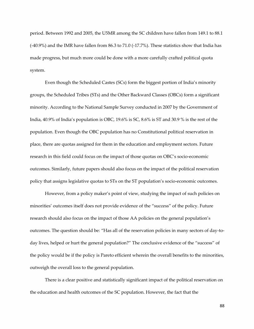
88
period. Between 1992 and 2005, the U5MR among the SC children have fallen from 149.1 to 88.1
(-40.9%) and the IMR have fallen from 86.3 to 71.0 (-17.7%). These statistics show that India has
made progress, but much more could be done with a more carefully crafted political quota
system.
Even though the Scheduled Castes (SCs) form the biggest portion of India’s minority
groups, the Scheduled Tribes (STs) and the Other Backward Classes (OBCs) form a significant
minority. According to the National Sample Survey conducted in 2007 by the Government of
India, 40.9% of India’s population is OBC, 19.6% is SC, 8.6% is ST and 30.9 % is the rest of the
population. Even though the OBC population has no Constitutional political reservation in
place, there are quotas assigned for them in the education and employment sectors. Future
research in this field could focus on the impact of those quotas on OBC’s socio-economic
outcomes. Similarly, future papers should also focus on the impact of the political reservation
policy that assigns legislative quotas to STs on the ST population’s socio-economic outcomes.
However, from a policy maker’s point of view, studying the impact of such policies on
minorities’ outcomes itself does not provide evidence of the “success” of the policy. Future
research should also focus on the impact of those AA policies on the general population’s
outcomes. The question should be: “Has all of the reservation policies in many sectors of day-to-
day lives, helped or hurt the general population?” The conclusive evidence of the “success” of
the policy would be if the policy is Pareto efficient wherein the overall benefits to the minorities,
outweigh the overall loss to the general population.
There is a clear positive and statistically significant impact of the political reservation on
the education and health outcomes of the SC population. However, the fact that the

89
Delimitation Commission has only met four times since the inception of the Constitution means
that the SC legislative seat proportion and the SC population proportion has been the same only
4 times in the past 67 years. Therefore, a major policy recommendation of this dissertation is
that the Government of India should find a way to equate the SC seat proportion and the SC
population proportion every year even if the Delimitation Commission might not meet that
often.

90
REFERENCES
Acharya, L., & Cleland, J. (2000). Maternal and child health services in rural Nepal: does access
or quality matter more?. Health Policy Plan, 15(2), 223–229.
Addisse, M. (2003, January). Maternal and Child Health Care. University of Gondar. Retrieved
from https://www.cartercenter.org/resources/pdfs/health/ephti/library/lecture_notes/
health_science_students/ln_maternal_care_final.pdf.
Anderson, T.W. & Hsiao, C. (1981). Estimation of Dynamic Models with Error Components.
Journal of the American Statistical Association, 76(375), 598-606.
Angloinfo.com (2015). The School System in India. India How to Guide: Family: Schooling and
Education. Retrieved from https://www.angloinfo.com/india/how-to/page/india-family-
schooling-education-school-system.
Arellano, M. & Bond, S. (1991). Some tests of specification for panel data: Monte Carlo evidence
and an application to employment equations. Review of economic studies, 58(2), 227-297.
Arellano, M. & Bover, O. (1995). Another look at the instrumental variables estimation of error
components models. Journal of Econometrics, 68(1), 29–51.
Arulampalam, W. & Bhalotra, S. (2004). Inequality in Infant Survival Rates in India:
Identification of State-Dependence Effects. Bristol Economics Discussion Papers,
Department of Economics, University of Bristol, UK. Retrieved from
http://EconPapers.repec.org/RePEc:bri:uobdis:04/558.
Atchoarena, D. & Gasperini, L. (2003). Education for rural development: towards new policy
responses. United Nations Educational, Scientific and Cultural Organization. Retrieved from
http://www.unesco.org/education/efa/know_sharing/flagship_initiatives/towards_new_
policy.pdf.
Badgett, M.V. L. (2014, February). The Economic Cost of Homophobia & the Exclusion of LGBT
People: A Case Study of India. The World Bank. Retrieved from
https://www.worldbank.org/content/dam/Worldbank/document/SAR/economic-costs
homophobia-lgbt-exlusion-india.pdf

91
Bardhan, P.K., Mookherjee, D., & Torrado, M. P. (2010). Impact of Political Reservations in West
Bengal Local Governments on Anti-Poverty Targeting. Journal of Globalization and
Development, 1(1), 1-38.
Besley, T., & Coate, S. (1997). An Economic Model of Representative Democracy. The Quarterly
Journal of Economics, 112(1), 85-114.
Besley, T., Pande, R., Rahman, L. and Rao, V. (2004). The Politics of Public Good Provision:
Evidence from Indian Local Governments. Journal of the European Economic Association,
2(2-3), 416–426.
Besley, T., Pande, R., & Rao, V. (2005, August). Political Selection and the Quality of
Government: Evidence from South India. LSE STICERD Research Paper No. PEPP08.
Retrieved from https://ssrn.com/abstract=1158330.
Bhalotra, S. (2007). Spending to save? State health expenditure and infant mortality in India.
Health Economics, 16(9), 911–928.
Bhalotra, S. (2008). Childhood Mortality and Economic Growth. The Centre for Market and Public
Organization, Department of Economics, University of Bristol, UK.
Bhalotra, S., Valente, C. & van Soest, A. (2008). Religion and Childhood Death in India.
The Centre for Market and Public Organization, Department of Economics, University of
Bristol, UK.
Bhalotra, S., & Soest, A. v. (2008). Birth-spacing, fertility and neonatal mortality in India:
Dynamics, frailty, and fecundity. Journal Of Econometrics, 143274(290).
Bhandari, L., & Dutta, S. (2007). Health Infrastructure in Rural India. Indian Institute of
Technology, Kanpur. Retrieved from
http://www.iitk.ac.in/3inetwork/html/reports/IIR2007/11-Health.pdf
Bicego, G. T., & Boerma, J. T. (1993). Maternal education and child survival: a comparative
study of survey data from 17 countries. Social Science & Medicine, 36(9), 1207.
Bloom, D. E. (2007). Education, Health and Development. American Academy of Arts and Sciences.
Retrieved from http://www.dphu.org/uploads/attachements/books/books_1474_0.pdf
Blundell, R., & Bond, S. (1998). Initial conditions and moment restrictions in dynamic panel data
models. Journal of Econometrics, 87(1), 115-143.
Bourne, K. L., & Walker, M. (1991). The Differential Effect of Mothers' Education on Mortality of
Boys and Girls in India. Population Studies, 45(2). 203.

92
Brockerhoff, M., & Derose, L. F. (1996). Child survival in East Africa: the impact of preventive
health care. World Development, 24(12), 1841.
Burns, C. (2012, March). The Costly Business of Discrimination. Center for American Progress.
Retrieved from https://www.americanprogress.org/wp-
content/uploads/issues/2012/03/pdf/lgbt_biz_discrimination.pdf
Cameron, A. & Trivedi, P. (2009). Microeconometrics Using Stata. Stata Press.
Chandra, R. (2005). Identity and Genesis of Caste System in India. Gyan Books.
Chatterjee, C., & Sheoran, G. (2007). Vulnerable groups in India The Centre for Enquiry into Health
and Allied Themes (CEHAT), 1-21.
Chattopadhyay, R., & Duflo, E. (2004). Women as Policy Makers: Evidence from a Randomized
Policy Experiment in India. Econometrica, 72(5). 1409.
Chauhan, P. (2016). Challenges Facing the Current Higher Education System in
India. International Journal of Engineering Technology Science and Research, 3(4).
Chin, A. & Prakash, N. (2011). The redistributive effects of political reservation for minorities:
Evidence from India. Journal of Development Economics, 96, 265-277.
Claeson, M., Bos, E., Mawji, T. & Pathmanathan, I. (2000). Reducing child mortality in India in
the new millennium. Bulletin of the World Health Organization, 78(10), 1192-1199.
Collett, D. (1994). Modelling Survival Time in Medical Research. Chapman and Hall, London.
Coughlan, J., Hooper, D. & Mullen, M. (2007). Structural Equation Modelling: Guidelines for
Determining Model Fit. Electronic Journal of Business Research Methods, 6(1).
Cox, D.R., & Oakes, D. (1984). Analysis of Survival Data. Chapman and Hall, London.
Croll, E. (2001). Endangered daughters: discrimination and development in Asia. Routledge
Das, N.P., Bhavsar, S. & Patel, R. (2000, November). The growth and development of scheduled
caste and scheduled tribe population in Gujarat and future prospects. International
Union for the Scientific Study of Population
Dawson, A. (2010). State capacity and the political economy of child mortality in developing
countries revisited: From fiscal sociology towards the rule of law. International Journal of
Comparative Sociology, 51(6), 403–422.

93
Deshpande, S. (2001, December). Caste and social structure. The Hindu. Retrieved from
http://www.thehindu.com/2001/12/06/stories/2001120600501000.htm
Downs, A. (1957). An Economic Theory of Democracy. Harper Collins Publishers.
Duflo, E. & Chattopadhyay, R. (2003). The impact of Reservation in the Panchayati Raj:
Evidence from a Nationwide Randomized Experiment. Economic and Political Weekly,
39(9).
Edlund, L. & Pande, R. (2002). Why Have Women Become Left-Wing? The Political Gender Gap
and the Decline in Marriage. Quarterly Journal of Economics, 117(3), 917-961.
Fang, H. & Moro, A. (2011). Theories of Statistical Discrimination and Affirmative Action: A
Survey. Handbook of Social Economics, 133–200.
Galanter, M. (1984). Competing Equalities: Law and the Backward Classes in India. University of
California Press
Ghurye, G.S. (1996). Caste and Race in India. Popular Prakashan.
Government of India. (2011). Educational Statistics at a Glance. Ministry of Human Resource
Development. Retrieved from
http://mhrd.gov.in/sites/upload_files/mhrd/files/statistics/EduStatGlance_2011.pdf
Government of India. (1950). The Constitution of India. Retrieved from
http://lawmin.nic.in/olwing/coi/coi-english/coi-4March2016.pdf
Government of India. (1961, 1971, 1981, 1991, 2001, 2011). Census of India Digital Library. The
Registrar General & Census Commissioner, India, New Delhi.
Grossman, M. (1972). On the Concept of Health Capital and the Demand for Health. Journal of
Political Economy, 80, 223-255.
Grossman, M. (1972). The demand for health: a theoretical and empirical investigation. National
Bureau of Economic Research. 74-135.
Gupta, M. D. (1990). Death Clustering, Mothers' Education and the Determinants of Child
Mortality in Rural Punjab, India. Population Studies, 44(3). 489.
Hanchinamani, B.B. (2001). Human Rights Abuses of Dalits in India. American University
Washington College of Law, 8(2), 18-19.

94
Hansen, L.P. (1982). Large sample properties of generalized method of moments estimators.
Econometrica, 50, 1029-1054.
Hill, K. (1999). Trends in child mortality in the developing world: 1960 to 1996. New York, NY:
UNICEF.
Holtz-Eakin, D., Newey, W., & Rosen, H. (1988). Estimating Vector Autoregressions with Panel
Data. Econometrica, 56(6), 1371-1395.
Houweling, A.J., Kunst, A.E., Looman, C., & Mackenbach, J. (2005) Determinants of under-5
mortality among the poor and the rich: A cross-national analysis of 43 developing
countries. International Journal of Epidemiology, 34 (6), 1257-1267.
Imai, K., Keele, L., & Tingley, D. (2010). A General Approach to Causal Mediation
Analysis. Psychological Methods, 15(4), 309
Innovations for Poverty Action. (2012). 2012 Annual Report. Retrieved from
https://www.poverty-
action.org/sites/default/files/publications/ipa_2012_annual_report.pdf
International Dalit Solidarity Network. (2007, March). India: UN Finds Pervasive Abuse Against
Dalits. Human Rights Watch. Retrieved from
https://www.hrw.org/news/2007/03/12/india-un-finds-pervasive-abuse-against-dalits
Iyer, L., Mani, A., Mishra, P., & Topalova, P. (2012). The Power of Political Voice: Women's
Political Representation and Crime in India. American Economic Journal: Applied
Economics, 4(4), 165-193.
Jaishankar, D. (2013, March). The Huge Cost of India’s Discrimination Against Women. The
Atlantic. Retrieved from http://www.theatlantic.com/international/archive/2013/03/the-
huge-cost-of-indias-discrimination-against-women/274115/
Jensenius, F. R. (2015). Development from Representation? A Study of Quotas for the Scheduled
Castes in India. American Economic Journal. Applied Economics, 7(3), 196-220.
Kishor, S., & Parasuraman, S. (1998). Mother’s employment and infant and child mortality in
India. International Institute for Population Sciences.
Krook, M., & Zetterberg, P. (2014). Electoral quotas and political representation: Comparative
perspectives. International Political Science Review, 35(1), 3-11.
Lott, J., & Kenny,L. (1999). Did Women's Suffrage Change the Size and Scope of Government?
Journal of Political Economy, 107(6), 1163-1198.

95
Madhok, R. (2013). Reservation Policy and Criminal Behavior in India: The Link Between
Political Reservation and Atrocities Against Scheduled Castes and Tribes. Issues in
Political Economy, 22, 56–76.
Masset, E., & White, H. (2003). Infant and Child Mortality in Andhra Pradesh: Analyzing
changes over time and between states. Munich Personal RePEc Archive.
Merick, T. (1985). The Effect of Piped Water on Early Childhood Mortality in Urban Brazil, 1970-
1976. Demography, 22(1), 1-14.
Mitra, A. (2015). Does mandated political representation help the poor? Theory and evidence
from India. Journal of Economic Literature.
Mosley, W.H., & Chen, L.C. (1984). An Analytical Framework for the Study of Child Survival in
Developing Countries. Population and Development Review, 10.
National Campaign on Dalit Human Rights. (2008). Alternate Report 2008. Retrieved from
http://www2.ohchr.org/english/bodies/cescr/docs/info-ngos/NCDHR-IDSNIndia40.pdf.
National University of Educational Planning and Administration. District Information System for
Education, New Delhi. Retrieved from http://www.dise.in
Osborne, M., & Slivinski, A. (1996). A Model of Political Competition with Citizen-
Candidates. The Quarterly Journal of Economics, 111(1), 65–96.
Palloni, A., & Tienda, M. (1986). The Effects of Breastfeeding and Pace of Childbearing on
Mortality at Early Ages. Demography. 23(1), 31-52.
Pande R. (2003). Can Mandated Political Representation Increase Policy Influence for
Disadvantaged Minorities? Theory and Evidence from India. The American Economic
Review, 93(4), 1132-1151
Papola, T. S. (2012). Social Exclusion and Discrimination in the Labor Market. Institute for Studies
in Industrial Development . Retrieved from http://isidev.nic.in/pdf/WP1204.pdf
Pebley, A.R., & Strupp, P.W. (1987). Reproductive Patterns and Child Mortality in Guatemala.
Demography, 24(1), 43-60.
Prakash, N., Rockmore, M., & Uppal, Y. (2015). Do Criminally Accused Politicians Affect
Economic Outcomes? Evidence from India. Households in Conflict Network (HiCN), The
Institute of Development Studies, University of Sussex.

96
Press Trust of India (PRI). (2015). Position of socially & financially deprived hasn’t improved:
Survey. The Economic Times. Retrieved from
http://articles.economictimes.indiatimes.com/2015-03-02/news/59684077_1_obc-rs-1514-
rs-1430
Reddy, D.S. (2005). The Ethnicity of Caste. Anthropological Quarterly, 78(3), 543-584.
Statistical Reports on State Elections in India. (1985 -2014). Election Commission of India New Delhi
Retherford D., Thapa S., & Gubhaju, B.B. (1989). To What Extent Does Breastfeeding Explain
Birth-Interval Effects on Early Childhood Mortality? Demography, 26(3), 439-450.
Robb, R., & Robb, A. (1999). Gender and the Study of Economics: The Role of Gender of the
Instructor. The Journal of Economic Education, 30(1), 3-19.
Saravanakumar, S., & Palanisamy, M. (2013). Status of Primary Education of Scheduled Caste
Children. International Journal of Research in Humanities and Social Sciences, 1(8).
Sebály, B. (2009, October). Sixty years on and caste discrimination continues in India. Minority
Rights Group International. Retrieved from http://minorityrights.org/2009/10/12/sixty-
years-on-and-caste-discrimination-continues-in-india/
Sen, A. (1999). Development as Freedom. Oxford, New York: Oxford University Press.
Shah, G., Mander, H., Thorat, S., Deshpande, S., & Baviskar, A. (2006). Untouchability in Rural
India. New Delhi: SAGE Publications, India Pvt Ltd.
Shirras, G. (1935). The Census of India, 1931. Geographical Review, 25(3), 434-448. Retrieved from
www.jstor.org/stable/209312.
Shiva Kumar, A. K. (1995). ‘Women’s Capabilities and Infant Mortality: Lessons from
Manipur’ In M. D. Gupta, L. Chen, and T. Krishnan (eds). Women’s Health in India:
Risk and Vulnerability. Oxford University Press: Bombay, 55–94.
Singh, D. (2009). Development of Scheduled Castes in India - A Review. Journal of Rural
Development Hyderabad, 28(4), 529-542.
Stapenhurst, F.C. (2004). The legislature and the budget. WBI working paper series. Washington,
DC: World Bank. Retrieved from http://documents.worldbank.org/curated/en/
835951468779433827/The-legislature-and-the-budget.
Sullivan, J.M., Rutstein, S.O., & Bicego, G.T. (1994). Infant and Child Mortality. Demographic and
Health Surveys Comparative Studies No. 15, Macro International Inc., Calverton, MD.

97
Tefft, S. (1990, February 8). Illiteracy Looms Over India. The Christian Science Monitor. Retrieved
from http://www.csmonitor.com/1990/0208/dteac.html.
Teltumbde, A. (1997). Impact of New Economic Reforms on Dalits in India. Occasional Paper
Series: 1, Department of Sociology, University of Pune, Pune. Retrieved from
http://www.unipune.ac.in/snc/cssh/HistorySociology/.
Teltumbde, A. (2001). Globalisation and the Dalits. Nagpur: Sanket Prakashan. Retrieved from
http://www.ambedkar.org/research/GLOBALISATIONANDTHEDALITS.pdf.
Thorat, S. (2007). Economic Exclusion and Poverty: Indian Experience of Remedies Against
Exclusion. Paper prepared for Policy Forum on Agricultural and Rural Development for
Reducing Poverty and Hunger in Asia: In Pursuit of Inclusive and Sustainable Growth, IFPRI,
and ADB, Manila, Philippines, August 9–10. Retrieved from
http://www.ifpri.org/2020ChinaConference/pdf/manilac_Thorat.pdf.
Thorat, S., & Deshpande, R. S. (1999). Caste and Labour Market Discrimination. The Indian
Journal of Labour Economics, 42(4), 841-854.
Thurlow, M. L., Sinclair, M. F., & Johnson, D. R. (2002, July). Students with disabilities who
drop out of school: Implications for policy and practice. Issue Brief: Examining Current
Challenges in Secondary Education and Transition, 1(2). Minneapolis, MN: Institute on
Community Integration, National Center on Secondary Education and Transition,
University of Minnesota.
United Nations. (2006). World population prospects: The 2004 revision. New York, NY: United
Nations. Retrieved from http://www.un.org/esa/population/publications/WPP2004/
WPP2004_Vol3_Final/WPP2004_Analytical_Report.pdf
Ushistory.org. (2016). The Caste System. Ancient Civilizations Online Textbook. Retrieved from
http://www.ushistory.org/civ/8b.asp.
Van den Berg, G.J., Bergemann, A., & Sumedha, G. (2010). Impact of an affirmative action
program in employment on child mortality in India. Beiträge zur Jahrestagung des Vereins
für Socialpolitik 2010: Ökonomie der Familie – Session: Skills, Risks, and Wages, No. E10-
V2.
William, A. (2014). Poverty as a Challenge. National Council of Educational Research and Training.
Retrieved from http://www.ncert.nic.in/ncerts/l/iess203.pdf
Windmeijer, F. (2005). A finite sample correction for the variance of linear efficient two-step
GMM estimators. Journal of Econometrics, 126(1), 25–51.

98
World Health Organization. (2000). The World Health Report 2000: Health systems: Improving
performance. Geneva: WHO. Retrieved from
http://www.who.int/whr/2000/en/whr00_en.pdf

99
APPENDIX A
Table 1.01: Literacy rate differentials among social groups in India
Census Year Total population literacy rate SC literacy rate
1961 24.0 10.3
1971 29.5 14.7
1981 36.2 21.4
1991 52.1 37.4
2001 65.4 54.7
2011 73.0 66.1
Source: Census of India Digital Library
Table 1.02: Enrollment rate differentials among social groups in India- primary school
Census Year India (%) SC population (%)
1961 24.02 10.27
1971 29.45 14.67
1981 36.23 21.38
1991 52.10 37.41
2001 65.00 54.69
Source: Ministry of Human Resource Development/ Census of India digital library. Note: The enrollment
rates (expressed as percentages) are the number of children enrolled in a level, divided by the
population of the age group that officially corresponds to the same level.

100
Table 1.03: Basic differentials among social groups
Indicators SC ST India
% Population below poverty line (2011) 29.4 43.0 22.0
Rural 31.5 45.3 25.4
Urban 21.7 24.1 13.7
Literacy rate (2011) 66.1 59.0 73.0
Male 75.2 68.5 80.9
Female 56.5 49.4 64.6
Gross enrollment ratio (GER)- primary
1990 106.4 104.0 100.1
2004 115.3 121.9 107.8
Gross enrollment ratio (GER)- upper primary
1990 52.7 40.7 62.1
2004 70.2 67.0 19.9
Dropout rates (grades 1-10)
1990 77.7 85.0 71.3
2004 71.3 79.0 61.9

101
Table 1.04: Summary Statistics- Education
Variable Obs Mean Std. Dev. Min Max
Gross Enrollment Ratio- primary (GERP) 476 105.84 31.22 11.02 160.57
Gross Enrollment Ratio- upper primary (GERUP) 486 74.59 25.02 12.63 119.73
Gross Enrollment Ratio- secondary (GERS) 157 71.71 28.28 12.13 151.15
Gross Enrollment Ratio- higher secondary
(GERHS)
160 46.96 22.79 1.92 99.98
SC reserved seats 666 20.62 20.99 0 91
Quota Share (QS) 663 0.828 0.354 0 1.81
SC per capita income 627 19098.95 14887.7 3985.9 106373.7
State’s education expenditure per pupil 576 9851880 9.86e07 2560.4 1.73e09
State’s welfare expenditure per capita 569 37604.04 221531.8 0 2740719
Number of primary schools 624 23624.7 26825.9 14 147376
Number of upper primary schools 627 8749.25 11864.2 7 96797
Number of secondary schools 180 4050.55 4753.2 63 19053
Number of higher secondary schools 180 2242.83 2278.8 48 10739

102
Table 1.05: Pairwise correlation among independent variables
Election
Year
SC per
capita
income
SC
population
density
SC Quota
Share
Education
expenditures
per pupil
Welfare
expenditure
per SC
Number
of
primary
schools
Number
of
upper-
primary
schools
Number
of
secondary
schools
Number of
higher
secondary
schools
Election Year 1.000
SC per capita
income -0.001 1.000
SC population
density 0.004 0.566 1.000
SC Quota Share 0.021 0.255 0.169 1.000
Education
expenditures per
pupil
-0.022 0.017 -0.037 -0.240 1.000
Welfare
expenditure per
SC
-0.0080 0.031 -0.062 -0.410 0.081 1.000
Number of
primary schools 0.006 -0.035 -0.188 0.182 -0.079 -0.155 1.000
Number of
upper-primary
schools
-0.020 -0.194 -0.194 0.165 -0.064 -0.119 0.709 1.000
Number of
secondary
schools
-0.024 -0.279 -0.215 0.119 -0.121 -0.148 0.602 0.582 1.000
Number of
higher
secondary
schools
0.007 -0.268 -0.141 0.241 -0.141 -0.189 0.810 0.738 0.697 1.000

103
Table 1.06: Fixed-effect – mediator variables (the mechanism)
Variables/Method FE (1) FE (2) FE(3) FE(4) FE (5) FE (6)
Log Quota Share (lag 1) 0.195**
(0.076)
0.386**
(0.181)
0.201
(0.618)
0.217
(0.422)
0.275
(0.965)
0.261
(0.561)
Log Quota Share (lag 2) 0.059
(0.088)
-0.017
(0.141)
0.732***
(0.157
1.97***
(0.124)
0.782*
(0.435)
0.087
(0.437)
Constant 8.99
(0.082)
7.53
(0.156)
7.18
(0.134)
6.00
(0.098)
9.66
(0.557)
7.97
(0.423)
State fixed effects Yes Yes Yes Yes Yes Yes
Year fixed effects Yes Yes Yes Yes Yes Yes
Number of observations 545 548 174 174 525 516
Number of groups 29 29 29 29 29 29
Overall R2 0.028 0.044 0.053 0.164 0.019 0.119
Note: Dependent variable are- log number of primary schools (column 1); log number of upper primary schools (column 2); log number of
secondary schools (column 3); log number of higher secondary schools (column 4); log state’s education expenditure (column 5); and log State’s
welfare expenditure (column 6) . Robust standard errors clustered with States are in parentheses. *, **, *** indicates statistical significance at α =
0.10, 0.05 and 0.01 respectively.

104
Table 1.07: Dynamic Panel model- GER- primary
Variables/Method One step System GMM
(1)
One step System GMM
(2)
Two step System
GMM (3)
Two step System
GMM (4)
Log SC Gross Enrollment Ratio- primary (lag 1) 0.958***
(0.026)
0.852***
(0.120)
0.958***
(0.027)
1.029***
(0.156)
Log quota share 0.387*
(0.193)
0.357**
(0.160)
0.384*
(0.199)
0.555***
(0.193)
Log SC income per capita 0.021
(0.043)
0.0034
(0.058)
Log number of primary schools (lag1) 0.018
(0.027)
-0.013
(0.048)
Log state education expenditure (lag1) 0.014
(0.031)
-0.036
(0.055)
SC population density -0.00005
(0.00006)
-0.00009
(0.00007)
Election Year -0.058
(0.071)
0.0001
(0.061)
Other mediator variables N Y N Y AR (1)
(p-value)
-2.73
(0.006)
-1.80
(0.071)
-2.64
(0.008)
-1.58
(0.115)
AR (2)
(p-value)
1.61
(0.108)
1.50
(0.133)
1.56
(0.118)
1.27
(0.205)
Hansen J-statistic
(p-value)
22.89
(0.691)
18.85
(0.988)
23.86
(0.638)
12.92
(0.954)
Hansen C-statistic
(p-value)
20.50
(0.365)
14.36
(0.996)
21.28
(0.321)
10.32
(0.502)
F-statistic 53245.55 37970.81 52521.28 113634.71
(p-value) (0.000) (0.000) (0.000) (0.000)
No. of instruments 29 42 29 30
No. of observations 401 308 401 308
Note: Dependent variable is Log SC Gross Enrollment Ratio- primary (GERP). Robust clustered standard errors are in parentheses. *, **, ***
indicates statistical significance at α = 0.10, 0.05 and 0.01 respectively. Column 1 and 3 excludes all of the mediator variables. Column 2 and 4
includes the mediator variables. Other mediator variables include States’ education expenditures, welfare expenditures and the interaction of
those variables with the quota variable.

105
Table 1.08: Dynamic Panel model- GER- upper primary
Variables/Method One step System
GMM (1)
One step System
GMM (2)
Two step system
GMM (3)
Two step system
GMM (4)
Log SC Gross Enrollment Ratio – upper primary
(lag 1)
0.769***
(0.162)
0.811***
(0.138)
0.402*
(0.204)
0.855**
(0.311)
Log quota share (lag 1) 0.200
(0.189)
0.275*
(0.147)
0.398*
(0.233)
0.764*
(0.439)
Log SC income per capita 0.024
(0.380)
0.0009
(0.089)
Log number of upper primary schools 0.027
(0.023)
0.016
(0.045)
Log state education expenditure 0.022
(0.047)
0.001
(0.064)
Election Year 0.032
(0.035)
0.072
(0.058)
Other mediator variables N Y N Y AR (1)
(p-value)
-2.11
(0.035)
-2.52
(0.012)
-1.91
(0.056)
-2.00
(0.046)
AR (2)
(p-value)
0.13
(0.900)
0.52
(0.600)
0.10
(0.918)
0.54
(0.589)
Hansen J statistic
(p-value)
16.51
(0.989)
13.40
(0.999)
11.49
(0.778)
13.44
(0.568)
Hansen C-statistic
(p-value)
11.75
(0.988)
14.47
(0.490)
5.98
(0.875)
3.73
(0.811)
F-statistic 71268.18 20927.62 59733.94 9446.49
(p-value) (0.000) (0.000) (0.000) (0.000)
No. of instruments 35 45 20 21
No. of observations 385 301 329 301
Note: Dependent variable is Log SC Gross Enrollment Ratio- upper primary (GERUP). Corrected standard errors are in parentheses. *, **, ***
indicates statistical significance at α = 0.10, 0.05 and 0.01 respectively. Column 1 and 3 are the results of one step and two system GMM
respectively and excludes all of the mediator variables. Column 2 and 4 includes the mediator variables.

106
Table 1.09: Dynamic Panel model- SC Gross secondary enrollment ratio (GERS)
Variables/Method One step System GMM
(1)
One step System GMM
(2)
Two step system GMM
(3)
Two step system GMM
(4)
Log SC secondary enrollment per capita
(lag 1)
0.823***
(0.049)
0.587***
(0.087)
0.823**
(0.051)
0.454***
(0.157)
Log quota share 1.218***
(0.296)
0.943*
(0.491)
1.203***
(0.292)
1.494
(0.990)
Log SC income per capita 0.180
(0.120)
0.004
(0.142)
Log number of secondary schools -0.037
(0.072)
0.118
(0.101)
SC population density
-0.0001
(0.0002)
0.0001
(0.0003)
Log welfare per capita
0.341**
(0.158)
Election Year -0.164*
(0.083)
-0.229
(0.186)
Other mediator variables N Y N Y AR (1)
(p-value)
-3.70
(0.000)
-2.93
(0.003)
-3.48
(0.001)
-1.90
(0.058)
AR (2)
(p-value)
-0.81
(0.419)
-1.19
(0.232)
-0.79
(0.427)
-0.54
(0.589)
Hansen J- statistic
(p-value)
24.33
(0.228)
18.86
(0.943)
24.33
(0.228)
46.42
(0.243)
Hansen C- statistic
(p-value)
23.50
(0.101)
14.68
(0.795)
23.50
(0.101)
5.40
(0.611)
F-statistic 17407.88 5023.67 7041.42 1636.58
(p-value) (0.000) (0.000) (0.000) (0.000)
No. of instruments 22 38 22 26
No. of observations 124 123 124 123
Note: Dependent variable is Log SC secondary school enrollment per capita. Corrected standard errors are in parentheses. *, **, *** indicates
statistical significance at α = 0.10, 0.05 and 0.01 respectively. Column 1 and 3 are the results of one step and two system GMM respectively and
excludes all of the mediator variables. Column 2 and 4 includes the mediator variables.

107
Table 1.10: Dynamic Panel model- SC Gross higher secondary enrollment ratio (GERHS)
Variables/Method One step System
GMM (1)
One step System
GMM (2)
Two step system
GMM (3)
Two step system
GMM (4)
Log SC higher secondary enrollment per
capita (lag 1)
0.591***
(0.087)
0.735***
(0.102)
0.493***
(0.102)
0.821***
(0.051)
Log quota share 0.819**
(0.307)
1.023*
(0.506)
1.651***
(0.389)
0.362*
(0.210)
Log SC income per capita
0.067
(0.099)
0.106*
(0.059)
Log education budget -0.024
(0.087)
-0.088
(0.053)
Log welfare budget 0.086
(0.074)
0.092
(0.061)
Literacy rate -0.0068
(0.0145)
-0.0021
(0.008)
Election Year 0.078
(0.072)
-0.235**
(0.110)
0.264***
(0.079)
-0.014
(0.086)
Other mediator variables N Y N Y AR (1)
(p-value)
-0.39
(0.695)
-2.77
(0.006)
-1.24
(0.216)
-2.53
(0.011)
AR (2)
(p-value)
-1.04
(0.298)
-1.02
(0.430)
-1.04
(0.296)
-1.58
(0.100)
Hansen J-statistic
(p-value)
20.64
(0.965)
18.49
(0.555)
18.69
(0.849)
23.70
(0.966)
Hansen C-statistic
(p-value)
16.60
(0.921)
15.91
(0.195)
18.52
(0.553)
23.76
(0.533)
F-statistic 5059.10 2500.13 3494.40 5065.59
(p-value) (0.000) (0.000) (0.000) (0.000)
No. of instruments 38 28 30 45
No. of observations 98 126 98 126
Note: Dependent variable is Log SC higher secondary school enrollment per capita. Corrected standard errors are in parentheses. *, **, ***
indicates statistical significance at α = 0.10, 0.05 and 0.01 respectively. Column 1 and 3 are the results of one step and two system GMM
respectively and excludes all of the mediator variables. Column 2 and 4 includes the mediator variables.

108
Table 1.11: Dynamic Panel model- SC Dropout rates
Variables/Method One step System
GMM – primary
(1)
Two step System
GMM – primary
(2)
Two step system
GMM- upper
primary (3)
One step System
GMM- secondary
(4)
Two step System
GMM- secondary
(5)
Log SC dropout rate (lag
1)
0.183
(0.179)
0.201
(0.224)
0.549**
(0.253)
0.314*
(0.171)
0.313*
(0.167)
Log quota share -4.256*
(2.179)
-4.139*
(2.422)
-5.247**
(2.239)
-2.23*
(1.33)
-1.877*
(0.987)
Log SC primary
enrollment per capita
-4.815
(5.814)
-3.412
(5.662)
Log SC income per
capita
0.415
(0.329)
0.354
(0.358)
0.142
(0.168)
-0.131
(0.239)
-0.139
(0.309)
Log number of schools 0.189
(0.158)
0.214
(0.157)
0.362*
(0.181)
0.576
(0.475)
0.572
(0.611)
Log student-teacher
ratio
0.473
(0.385)
0.355
(0.511)
0.223
(0.236)
0.217
(0.265)
Election Year 0.108
(0.266)
0.165
(0.243)
-0.0267
(0.110)
AR (1)
(p-value)
-1.35
(0.178)
-1.07
(0.284)
-1.44
(0.150)
-1.74
(0.081)
-1.61
(0.107)
AR (2)
(p-value)
-0.66
(0.508)
-0.55
(0.582)
-1.02
(0.310)
Hansen
(p-value)
17.27
(0.635)
17.27
(0.635)
17.80
(0.962)
19.34
(0.500)
19.34
(0.500)
Hansen Diff
(p-value)
-1.98
(0.999)
-1.98
(0.999)
-3.05
(0.999)
1.30
(0.730)
1.30
(0.730)
No. of instruments 27 27 35 25 25
No. of observations 141 141 211 91 91
Note: Dependent variable is Log of dropout rates. Corrected standard errors are in parentheses. *, **, *** indicates statistical
significance at α = 0.10, 0.05 and 0.01 respectively.

109
Table 1.12: Robustness check- DPD with district level data
Variables SC Primary
enrollment (1)
SC upper primary
enrollment (2)
Log SC enrollment per capita (lag 1) 0.915***
(26.97)
0.646***
(0.102)
Log quota share (lag 1) 0.106*
(0.059)
0.832***
(0.214)
AR (1)
(p-value)
--2.35
(0.019)
-2.90
(0.004)
AR (2)
(p-value)
1.48
(0.139)
-0.61
(0.540)
Hansen
(p-value)
8.23
(0.411)
1.57
(0.667)
Hansen Diff
(p-value)
0.48
(0.924)
1.14
(0.566)
No. of instruments 10 5
No. of observations 2924 2958
Note: Dependent variables are Log SC primary and upper primary enrollments per capita. Corrected standard errors are in
parentheses. *, **, *** indicates statistical significance at α = 0.10, 0.05 and 0.01 respectively. Both columns 1 and 2 are the results of
two step system GMM
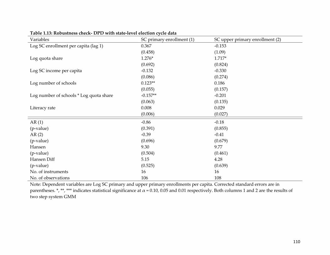
110
Table 1.13: Robustness check- DPD with state-level election cycle data
Variables SC primary enrollment (1) SC upper primary enrollment (2)
Log SC enrollment per capita (lag 1) 0.367
(0.458)
-0.153
(1.09)
Log quota share 1.276*
(0.692)
1.717*
(0.824)
Log SC income per capita -0.132
(0.086)
-0.330
(0.274)
Log number of schools 0.123**
(0.055)
0.186
(0.157)
Log number of schools * Log quota share -0.157**
(0.063)
-0.201
(0.135)
Literacy rate 0.008
(0.006)
0.029
(0.027) AR (1)
(p-value)
-0.86
(0.391)
-0.18
(0.855)
AR (2)
(p-value)
-0.39
(0.696)
-0.41
(0.679)
Hansen
(p-value)
9.30
(0.504)
9.77
(0.461)
Hansen Diff
(p-value)
5.15
(0.525)
4.28
(0.639)
No. of instruments 16 16
No. of observations 106 108
Note: Dependent variables are Log SC primary and upper primary enrollments per capita. Corrected standard errors are in
parentheses. *, **, *** indicates statistical significance at α = 0.10, 0.05 and 0.01 respectively. Both columns 1 and 2 are the results of
two step system GMM

111
Table 1.14: Robustness Check- DPD without UTs & newer states
Variables GPER (1) GPER (2) GUPER (3) GUPER (4)
Log SC enrollment per capita (lag 1) 1.062***
(0.115))
-0.021
(0.148)
0.843***
(0.089)
0.265
(0.462)
Log quota share 0.079**
(0.032)
2.727***
(0.944)
0.108*
(0.057)
2.274*
(1.333)
Log SC income per capita -0.200*
(0.103)
-0.189**
(0.084)
Log number of schools 0.099
(0.088)
0.091
(0.119)
Log number of schools * Log quota share -0.159
(0.116)
-0.204
(.0130)
Literacy rate -0.0005*
(0.0003)
SC population density -0.00002
(0.00003)
0.0003
(0.0007)
-0.00003
(0.0001)
-0.0005
(0.0007)
Election Year dummy -0.0165*
(0.0087)
0.0016
(0.008)
0.0333
(0.0379)
-0.0334
(0.029)
Other mediator variables N Y N Y AR (1)
(p-value)
-2.63
(0.009)
-1.06
(0.290)
-3.33
(0.001)
-1.39
(0.166)
AR (2)
(p-value)
1.43
(0.151)
-0.20
(0.841)
0.77
(0.443)
0.97
(0.330)
Hansen
(p-value)
16.42
(0.355)
5.80
(0.760)
16.93
(0.260)
5.59
(0.992)
Hansen Diff
(p-value)
7.93
(0.440)
2.48
(0.779)
4.65
(0.589)
-1.26
(0.999)
No. of instruments 21 20 18 28
No. of observations 442 342 474 335
Note: Dependent variables are Log SC primary enrollments per capita (column 1 and 2) and upper primary enrollments per capita (column 3 and
4). Corrected standard errors are in parentheses. *, **, *** indicates statistical significance at α = 0.10, 0.05 and 0.01 respectively. All the estimates
are the results of two step system GMM.

112
Table 2.01: Summary statistics of covariates of the hazard model
All survey sample Scheduled Caste
Categorical Variables Frequency (N) Percent (%) Frequency (N) Percent (%)
Gender of child
Male 133,435 51.96 25,495 51.66
Female 123,348 48.04 23,857 48.34
Religion
Hindu 182,752 71.17
Muslim 39,955 15.56
Place of residence
Urban 101,981 39.72 18,336 37.15
Rural 154,788 60.28 31,016 62.85
Caste
SC 45,486 18.94
ST 36,794 14.95
OBC 86,033 34.84
Mother’s education
No education 131,634 51.26 31,634 64.10
Some education 125,148 48.74 17,718 35.90
Wealth Index
Poorest 41,057 15.99 10,684 21.65
Poorer 45,707 17.82 10,898 22.08
Richer 57,827 22.52 9,996 20.25
Richest 59,342 23.12 6,736 13.65
Quota
< 50% 14,535 6.47 908 2.02
50-60% 10,444 4.65 1,893 4.22
60-70% 6,154 2.74 968 2.16
70-80% 5,498 2.45 1,132 2.52
80-90% 49,474 22.03 10,586 23.61
Breastfed the child
No 196,593 76.56 37,055 75.08
Yes 60,190 23.44 12,297 24.92
Place of delivery
Home 23,308 11.04 6,029 12.22
Government facility 9,830 3.83 1,929 3.91
Private facility 10,676 4.16 1,353 2.74
Access to health care
Not a big problem 188,925 73.59 35,761 72.48
Big problem 67,795 26.41 13,576 27.52
ORS
Never heard of it 67,482 26.28 14,271 28.92
Have used it 4,668 1.82 758 1.54
Antenatal care
Yes 29,631 11.54 5,309 10.76
No 6,815 2.65 1,350 2.74
Immunized against tetanus
No 5,453 2.12 1,103 2.23
Yes 30,994 12.07 5,578 11.30
Fuel used for cooking
Safe 80,948 31.52 11,553 23.41
Unsafe 168,475 65.61 36,336 73.63
Toilet
Unsanitary 24,728 9.63 2,906 5.89
No toilet 110,932 43.20 27,928 56.59
Water source
Safe 231,126 90.01 46,070 93.35
Unsafe 17,769 6.92 1,651 3.35

113
Table 2.02: Test of proportional hazard assumption- IMR
rho chi^2 df P>chi^2
Religion 0.0342 1.27 1 0.259
Breastfed 0.0321 1.27 1 0.259
Access to health
care
0.0529 2.91 1 0.088
Birth order 0.0181 0.35 1 0.552
Mother’s age 0.0218 0.54 1 0.464
Type of residence -0.0128 0.16 1 0.687
Gap between
births
0.0202 0.70 1 0.401
Wealth Index -0.0446 1.95 1 0.163
Quota 0.0035 0.02 1 0.892
ORS -0.0238 0.50 1 0.479
Antenatal care 0.0438 2.39 1 0.122
Access to water -0.0220 0.55 1 0.459
GLOBAL 16 12 0.191
Table 2.03: Test of proportional hazard assumption- U5MR
rho chi^2 df P>chi^2
Breastfed 0.0294 2.33 1 0.127
Access to
health care
0.0255 1.60 1 0.206
Type of
residence
0.0153 0.56 1 0.455
Gender 0.0413 4.15 1 0.042
Quota 0.0226 1.95 1 0.163
ORS 0.0109 0.21 1 0.650
Antenatal
care
0.0153 0.70 1 0.402
Access to
water
-0.0067 0.12 1 0.732
GLOBAL 13.58 8 0.094

114
Table 2.04: Chi-square test of independence of categorical variables
Variables Water Toilet Fuel Tetanus Antenatal
care
ORS Access
to
health
care
Place of
delivery
Religion
Water 6.631
(0.036)
0.901
(0.343)
2.631
(0.105)
2.631
(0.105)
0.262
(0.877)
2.619
(0.106)
1.609
(0.447)
31.908
(0.000)
Toilet 6.631
(0.036)
62.860
(0.000)
1.741
(0.419)
1.081
(0.582)
15.763
(0.003)
15.871
(0.000)
34.071
(0.000)
8.255
(0.220)
Fuel 0.901
(0.343)
62.860
(0.000)
4.971
(0.027)
4.971
(0.027)
8.788
(0.012)
4.534
(0.033)
24.274
(0.000)
4.902
(0.179)
Tetanus 2.631
(0.105)
1.741
(0.419)
4.971
(0.027)
92.401
(0.000)
1.126
(0.569)
11.264
(0.001)
5.821
(0.054)
19.665
(0.000)
Antenatal
care
2.631
(0.105)
1.081
(0.582)
4.971
(0.027)
92.401
(0.000)
1.126
(0.569)
1.950
(0.163)
5.821
(0.054)
19.665
(0.000)
ORS 0.262
(0.877)
15.763
(0.003)
8.788
(0.012)
1.126
(0.569)
1.126
(0.569)
0.091
(0.956)
7.677
(0.104)
1.416
(0.965)
Access to
health
care
2.619
(0.106)
15.871
(0.000)
4.534
(0.033)
11.264
(0.001)
1.950
(0.163)
0.091
(0.956)
9.710
(0.008)
26.315
(0.000)
Place of
delivery
1.609
(0.447)
34.071
(0.000)
24.274
(0.000)
5.821
(0.054)
5.821
(0.054)
7.677
(0.104)
9.710
(0.008)
6.245
(0.396)
Religion 31.908
(0.000)
8.255
(0.220)
4.902
(0.179)
19.665
(0.000)
19.665
(0.000)
1.416
(0.965)
26.315
(0.000)
6.245
(0.396)

115
Table 2.05: Cox Regression for IMR
IMR (1) IMR (2) IMR (3) IMR (4) IMR (5) IMR (6)
Quota Share
(lag 2)
50-60%
60-70%
70-80%
80-90%
-1.157***
(0.317)
-0.295
(0.293)
-1.422***
(0.376)
-0.510
(0.347)
-0.836**
(0.342)
-0.562**
(0.236)
-1.312***
(0.326)
-0.470
(0.295)
-0.438
(0.269)
-0.402**
(0.208)
-1.487***
(0.373)
-0.562*
(0.346)
-0.902***
(0.339)
-0.628***
(0.234)
-1.479***
(0.364)
-0.519
(0.344)
-0.884***
(0.337)
-0.645***
(0.233)
-1.536***
(0.373)
-0.603*
(0.346)
-0.954***
(0.339)
-0.674***
(0.233)
Behavioral
variables
No No Yes Yes Yes Yes
Biological
variables
No Yes No Yes Yes Yes
Environmental
variables
No Yes Yes No Yes Yes
Socio-
economic
variables
No Yes Yes Yes No Yes
Wealth Index
Poorest
Poorer
Richer
Richest
0.425***
(0.126)
0.399***
(0.124)
-0.074
(0.154)
-0.412***
(0.219)
0.545***
(0.081)
0.433***
(0.078)
-0.061
(0.089)
-0.462***
(0.115)
0.459***
(0.096)
0.413***
(0.093)
-0.062
(0.108)
-0.388***
(0.142)
0.443***
(0.093)
0.406***
(0.093)
-0.064
(0.108)
-0.394***
(0.142)
Number of
observations
40268 27974 40258 27986 27992 27986
Number of
deaths
1480 1036 1478 1036 1038 1036
Log likelihood -15594.74 -10307.06 -15444.47 -10298.91 -10345.51 -10293.91
Wald chi2 (p-
value)
72.54
(0.000)
3052.76
(0.000)
4973.50
(0.000)
2935.49
(0.000)
305.46
(0.000)
2982.50
(0.000)
Note: The coefficients are the β coefficients, not the hazard ratios. The hazard ratio is given as exp(β). The
standard errors are robust standard errors. *, **, *** represent 10%, 5% and 1% significance level
respectively.

116
Table 2.06: Cox Regression for U5MR
U5MR (1) U5MR (2) U5MR (3) U5MR (4) U5MR (5) U5MR (6)
Quota Share
(lag 2)
50-60%
60-70%
70-80%
80-90%
-1.096***
(0.253)
-0.593**
(0.256)
-1.182***
(0.296)
-0.717**
(0.313)
-0.480*
(0.259)
-0.483**
(0.199)
-1.212***
(0.258)
-0.702***
(0.258)
-0.360*
(0.213)
-0.429**
(0.169)
-1.220***
(0.293)
-0.738**
(0.312)
-0.509**
(0.257)
-0.520***
(0.197)
-1.312***
(0.289)
-0.763**
(0.313)
-0.518**
(0.256)
-0.568***
(0.198)
-1.274***
(0.293)
-0.781**
(0.312)
-0.566**
(0.257)
-0.572***
(0.197)
Behavioral
variables
No No Yes Yes Yes Yes
Biological
variables
No Yes No Yes Yes Yes
Environmental
variables
No Yes Yes No Yes Yes
Socio-economic
variables
No Yes Yes Yes No Yes
Wealth Index
Poorest
Poorer
Richer
Richest
0.604***
(0.072)
0.429***
(0.072)
-0.147*
(0.086)
-0.488***
(0.112)
0.658***
(0.062)
0.422***
(0.062)
-0.137*
(0.072)
-0.531***
(0.093)
0.623***
(0.073)
0.434***
(0.073)
-0.132
(0.086)
-0.457***
(0.112)
0.607***
(0.073)
0.426***
(0.073)
-0.134
(0.086)
-0.464***
(0.112)
Number of
observations
40268 27974 40258 27986 27992 27986
Number of
deaths
2422 1766 2420 1766 1768 1766
Log likelihood -25373.22 -17473.99 -25099.41 -17457.91 -17537.61 -17448.64
Wald chi2 (p-
value)
156.18
(0.000)
5062.28
(0.000)
7415.42
(0.000)
5001.19
(0.000)
513.48
(0.000)
5088.27
(0.000)
Note: The coefficients are the β coefficients, not the hazard ratios. The hazard ratio is given as exp(β). The
standard errors are robust standard errors. *, **, *** represent 10%, 5% and 1% significance level
respectively.

117
Table 2.07: Cox Regression for IMR – by residence
IMR (1) IMR (2)
Rural Urban Rural Urban
Quota Share
50-60%
60-70%
70-80%
80-90%
-1.629***
(0.615)
-0.559
(0.495)
-0.556
(0.433)
-0.579*
(0.341)
-1.733***
(0.487)
-0.845*
(0.498)
-1.906***
(0.668)
-0.812**
(0.325)
-0.961*
(0.592)
0.198
(0.437)
0.484
(0.381)
0.310
(0.326)
-1.395***
(0.380)
-0.768*
(0.401)
-0.777*
(0.451)
-0.568**
(0.265)
Behavioral variables Yes Yes No No
Biological variables Yes Yes No No
Environmental variables Yes Yes No No
Socio-economic variables Yes Yes No No
Wealth Index
Poorest
Poorer
Richer
Richest
0.500***
(0.116)
0.465***
(0.114)
-0.079
(0.169)
-0.591*
(0.332)
0.181
(0.235)
0.214
(0.186)
-0.100
(0.148)
-0.433**
(0.173)
Number of observations 17478 10508 24601 15667
Number of deaths 705 331 992 488
Log likelihood -6658.54 -2969.24 -9956.39 -4685.33
Wald chi2 (p-value) 1824.87
(0.000)
729.68
(0.000)
54.77
(0.000)
22.88
(0.001)
Note: The coefficients are the β coefficients, not the hazard ratios. The hazard ratio is given as exp(β). The
standard errors are robust standard errors. *, **, *** represent 10%, 5% and 1% significance level
respectively.

118
Table 2.08: Cox Regression for U5MR – by residence
U5MR (1) U5MR (2)
Rural Urban Rural Urban
Quota Share
50-60%
60-70%
70-80%
80-90%
-1.775***
(0.527)
-0.710*
(0.422)
-0.363
(0.332)
-0.515*
(0.275)
-1.232***
(0.383)
-1.024**
(0.474)
-1.047**
(0.444)
-0.664**
(0.285)
-1.356***
(0.509)
-1.608
(0.361)
-1.203***
(0.304)
-1.048***
(0.369)
-0.625*
(0.327)
-0.551**
(0.226)
Behavioral variables Yes Yes No No
Biological variables Yes Yes No No
Environmental variables Yes Yes No No
Socio-economic variables Yes Yes No No
Wealth Index
Poorest
Poorer
Richer
Richest
0.680***
(0.089)
0.522***
(0.090)
-0.139
(0.138)
-0.519**
(0.256)
0.389**
(0.164)
0.183
(0.142)
-0.208*
(0.114)
-0.558***
(0.134)
Number of observations 17478 10508 24601 15667
Number of deaths 1210 556 1645 777
Log likelihood -11353.97 -4977.09 -16401.89 -7423.74
Wald chi2 (p-value) 2489.17 (0.000) 49285.81 (0.000) 111.75 (0.000) 40.98 (0.002)
Note: The coefficients are the β coefficients, not the hazard ratios. The hazard ratio is given as exp(β). The
standard errors are robust standard errors. *, **, *** represent 10%, 5% and 1% significance level
respectively.

119
APPENDIX B
Figure 1.1: Literacy rate differentials among social groups
Figure1.2: Gross enrollment ratio (GER)- primary schools

120
Figure 1.3: Sample box-plot and regression coefficients for all levels of schooling- one-step
system GMM
Figure 1.4: Sample box-plot and regression coefficients for all levels of schooling- two-step
system GMM

121
Figure 2.1: Data censoring illustration for hazard model- IMR
Figure 2.2: Data censoring illustration for hazard model- U5MR

122
Figure2.3: SC children proportion surviving against survival time in months- by quota quintile
0.5
10
.51
0 100 200 300 400
QD = 1 (<50%) QD = 6 (50-60%) QD = 7 (60-70%)
QD = 8 (70-80%) QD = 9 (80-90%)
Pro
po
rtio
n S
urv
ivin
g
survivaltimeGraphs by quota quintile

123
Figure 2.4: Kaplan-Meier hazard plot- IMR
Figure 2.5: Kaplan-Meier hazard plot- U5MR
ST
SC
OBC
Others
0.0
00
.01
0.0
20
.03
0.0
40
.05
0 5 10 15Survival time (months)
Kaplan-Meier IMR estimates

124
Figure 2.6: Kaplan Meier hazard plot- U5MR by sex (All India)
Figure 2.7: Kaplan Meier hazard plot- U5MR by sex (SC)
125
Figure 2.8: Kaplan Meier hazard plot- U5MR by sex (Others)

126
APPENDIX C: An alternative approach: The Structural Equation Model
To understand the mechanism through which the political reservation affects the
education outcomes of SC, I use the mediation analysis with Structural Equation Model (SEM).
SEM allows us to test the hypotheses about the relationship among different variables
simultaneously. Hence, it is a multivariate technique that allows us to estimate a system of
equations as a tool to estimate both the direct and indirect effects of the variable of interest on
the dependent variable. It fits models using the observed covariances and the means. However,
the use of SEM requires us to have a set of assumptions. First, the sample size has to be “large”.
The SEM model uses the Maximum Likelihood (ML) estimator. Since ML estimation relies on
asymptotics, large sample size is required to get a consistent/efficient estimation of parameters.
My data supports this assumption as I have an average of 640 observations per variable in my
unbalanced panel data. Secondly, the SEM model assumes that the observed variable follow a
multivariate normal distribution because the likelihood that is being maximized in the
structural equation model uses the ML estimation. However, this assumption can be relaxed for
the exogenous variables in the model. Finally, the SEM model assumes that there are no
relevant variables that are omitted from the model -- i.e. the model is correctly specified. Thus,
if the model is not fully specified, it might be prone to omitted variable bias, as in the linear
regression case. This is one of the shortcomings in this SEM analysis as it is very hard to identify
a complete path with all the possible variables. Therefore, this method is expected to have some
bias on the coefficient estimates. However, the mediator variables are chosen based on the
possible quantifiable mediation effect of QS on enrollments.
Mediation analysis is a part of the SEM model with which one can understand the
underlying mechanism of a relationship between a dependent and independent variable
through one or more mediator variables. It is important to understand, however, that because of

127
limitation in fully specifying the model paths, the mediation model might not test the direct
causal relationship between the dependent and independent variable. Instead, it treats the
independent variable as the main cause of mediator variables, which in-turn causes the
dependent variable (as depicted in the figure below.) Thus, the mediator variable explains the
relationship between the dependent and the independent variable.
α β
γ
Figure above shows a simple mediation SEM model where the independent variable (X)
causes the mediator variable (M), which in-turn causes the dependent variable (Y). Hence, there
is a direct effect of X on Y and also an indirect effect from X to M to Y. In the figure above, direct
effect = γ, indirect effect = αβ and the total effect = γ + αβ. The following path diagram describes
the perceived relationships between different variables which are modeled to analyze the
presence and the extent of the impact that mediator variables have in my study. I am interested
in the direct, indirect, and the total effects of the QS on two of my dependent variables (SCPEPC
and SCUPEPC).
In the path diagram Figure 1.15 and Figure 1.16 (below), the independent variable of
interest is LnQS (natural log of QS) and the two dependent variables are the LnSCPEPC and
LnSCUPEPC (natural logs of SC primary and SC upper primary enrollments per capita). The
mediator variables in the path diagram are STRP, LnNoPS, LnEBPP, LnWBPC, LnNoUPS and
STRUP (described above). We can also see that LnQS can be affected by the ‘ElectionYear’ and
the ‘SCPopDensity’ variables because of the way that the quota is assigned. Since the income of
the SC families might have an impact on the primary and upper primary enrollments,
LnSCPCInc is also included in the model.
Independent
variable (X)
Mediator variable
(M)
Dependent
variable (Y)
E1
E2

128
The estimates from the Structural Equation Model (SEM) are provided in Table 1.15 and
Table 1.16 below. Since the robust clustered standard errors are used, the goodness of fit for the
SEM model is given by the Standardized root mean squared residuals (SRMR). The coefficient
of determination and the overall R2 are also calculated. All of these test results are included on
tables 1.15 and 1.16. Tables 1.15 and 1.16 also contain the direct, indirect and total effects of
quotas and other variables on the SC enrollments in primary and upper primary schools
respectively. Column 1 of Table 1.15 provides the direct effect of quotas and other variables on
primary school enrollment. As expected, the direct impact of quotas on the enrollment rate of
SC in primary education is positive and significant. It suggests that a 10% increase in the Quota
Share (QS) will increase the enrollment in primary education by 3.3% and it is significant at the
10% level. Similarly, column 2 of Table 1.15 shows the indirect effect of quotas on enrollment.
The indirect effects come from the various mediator variables previously described in the path
diagram. The results suggest that a 10% increase in QS will result in a 9.34% increase in the SC
enrollment in primary education and is significant at the 1% level. Finally, column 3 shows the
total effects of QS and other control variables on the SC enrollment. It shows that a 10% increase
in QS will likely increase the SC enrollment in primary education by about 13%. The coefficient
is significant at the 1% level. It is also important to highlight the significance of the proposed
mediator variables. The results listed in column 1 show that the number of schools, the
education budget, and the welfare budget all play a significant mediating role. For example, a
1% increase in QS will likely increase in the number of primary schools by 14.4%, an increase in
the education budget by 14.7%, and an increase in the welfare budget by 9.23%, all of which
lead to an increase in SC primary school enrollment rates.
As previously stated, Table 1.16 provides the SEM results for SC upper primary
enrollment rates. Column 1 provides the direct effect of quotas and other variables on the upper
primary enrollment. As expected, the direct impact of quotas on the enrollment of SC in upper
primary education is positive and small. However, it is not statistically significant. Similarly,
column 2 shows the indirect effect of quotas on enrollment. The indirect effects come from the

129
various mediator variables previously described in the path diagram. The SEM results suggest
that a 10% increase in QS will result in a 6.9% increase in the SC upper primary school
enrollment; this is significant at the 1% level. Finally, column 3 shows the total effects of QS and
other control variables on the SC enrollment rate. It shows that a 10% increase in QS will likely
increase the SC enrollment rate in upper primary education by about 10%. The coefficient is
significant at the 1% level. As before, the role of mediator variables is important to highlight.
The results listed in column 1 show that the number of schools, the education budget, and the
welfare budget all play a significant mediating role. For example, a 1% increase in QS will most
likely increase the number of upper primary schools by 12.5%, the education budget by 14.8%,
and the welfare budget by 9.5%.

130
Figure 1.5: SEM path diagram for SC primary enrollment rates
LnQS
1
LnNoPS 2
LnEBPP 3
LnWBPC 4
LnSCPEPC
5
NoPS*QS
SCPopDensity
EBPP*QS
ElectionYear
WBPC*QS
Structural Equation Model: Path Diagram for primary enrollments

131
Figure 1.6: SEM path diagram for SC upper primary enrollment rates
LnQS
1
LnNoUPS 2
LnEBPP 3
LnWBPC 4
LnSCUPEPC
5
NoUPS*QS
SC Pop Density
EBPP*QS
LnSCIncPC
Election Year
WBPC*QS
LnSTRUP 6
Literacy rate
Structural Equation Model: Path Diagram for upper primary enrollment

132
Table 1.15: Alternate method- Mediation analyzing using Structural Equation Model- primary enrollment rates
Model SEM (1) Direct effects Indirect effects Total effects
LnNoPS <- LnQS 14.43***
(0.687)
LnEBPP <- LnQS 14.72***
(0.392)
LnWBPC <- LnQS 9.23***
(0.434)
LnSCPEPC <-LnQS 0.333*
(0.197)
0.333*
(0.197)
0.934***
(0.030)
1.267***
(0.185)
LnNoPS 0.519***
(0.010)
0.052***
(0.011)
0.052***
(0.011)
LnEBPP 0.063***
(0.024)
0.064***
(0.024)
0.064***
(0.024)
LnWBPC -0.082***
(0.027)
-0.082***
(0.027)
-0.082***
(0.027)
SCPD -0.00005***
(0.00001)
-0.00005***
(0.00001)
0.0008**
(0.0004)
0.0008*
(0.0003)
Election Year 0.696***
(0.110)
0.696***
(0.110)
LnNoPS * LnQS -0.079***
(0.018)
-0.079***
(0.018)
-0.079***
(0.018)
LnEBPP * LnQS -0.079**
(0.032)
-0.079**
(0.033)
-0.079**
(0.033)
LnWBPC * LnQS 0.155***
(0.044)
0.155***
(0.044)
0.155***
(0.044)
Note: Number of observations = 445. Robust standard errors are clustered at the state level and are reported in parentheses. *, **, *** indicates
statistical significance at α = 0.10, 0.05 and 0.01 respectively. Coefficient of determination (CD) = 0.856; Standardized root mean squared residuals
(SRMR) = 0.487; R2 = 0.856 Refer to APPENDIX FIGURE 1.15 for the corresponding path diagram.

133
Table 1.16: Alternate method- Mediation analyzing using Structural Equation Model- upper primary enrollment rates Model SEM (2) Direct effects Indirect effects Total effects LnNoUPS <- LnQS 12.54***
(0.733)
LnEBPP <- LnQS 14.83*** (0.372)
LnWBPC <- LnQS 9.45*** (0.402)
LnSTRUP <- LnQS 5.11*** (0.168)
LnSCUPEPC <-LnQS 0.318 (0.326)
0.318 (0.326)
0.688*** (0.028)
1.005*** (0.336)
LnNoUPS 0.053** (0.027)
0.053** (0.027)
0.053** (0.027)
LnEBPP 0.085 (0.055)
0.085 (0.055)
0.085 (0.055)
LnWBPC -0.107* (0.064)
-0.107* (0.064)
-0.107* (0.064)
LnSTRUP -0.043** (0.022)
-0.043** (0.022)
-0.043** (0.022)
SCPD -0.00006*** (0.00002)
-0.00006*** (0.00002)
0.0007 (0.0006)
0.0006 (0.0006)
LnSCIncPC -0.040 (0.031)
-0.040 (0.031)
-0.040 (0.031)
Literacy rate 0.007*** (0.001)
0.007*** (0.001)
0.007*** (0.001)
Election Year 0.598 (0.477)
0.598 (0.477)
LnNoUPS * LnQS -0.064* (0.039)
-0.064* (0.039)
-0.064* (0.039)
LnEBPP * LnQS -0.112* (0.066)
-0.112* (0.066)
-0.112* (0.066)
LnWBPC * LnQS 0.167* (0.092)
0.167* (0.092)
0.167* (0.092)
Note: Number of observations = 313. Robust standard errors are clustered at the state level and are reported in parentheses. *, **, *** indicates
statistical significance at α = 0.10, 0.05 and 0.01 respectively. Coefficient of determination (CD) = 0.867; Standardized root mean squared residuals
(SRMR) = 0.367; R2 = 0.867 Refer to APPENDIX FIGURE 1.16 for the corresponding path diagram.