University of Jyväskylä

Department of Mathematical Information Technology

Edris Aman

Bridging Data Mining and Semantic Web

Master’s Thesis in Information Technology

23. Septemberta 2016

1

Author: Edris Aman

Contact information: edrismuzemil@gmail.com

Supervisor: Vagan Terziyan & Khriyenko Oleksiy

Title in English: Bridging Data Mining and Semantic Web

Työn nimi: Bridging Data Mining and Semantic Web

Project: Master’s Thesis in Information Technology

Page Count: 65

Abstract: Nowadays Semantic Web is widely adopted standard of knowledge representa-

tion. Hence, knowledge engineers are applying sophisticated methods to capture, discover

and represent knowledge in Semantic Web form. Studies show that, to represent

knowledge in Semantic Web standard, data mining techniques such as Decision Trees,

Association Rules, etc., play an important role. These techniques are implemented in pub-

licly available Data Mining tools. These tools represent knowledge discovered in hu-

man readable format and some tools use Predictive Model Markup language (PMML).

PMML is an XML based model for data mining model representation that fails to address

the representation of the semantics of the discovered knowledge. Hence, this thesis tries to

research and give solutions to translate PMML to Semantic Web Rule Language (SWRL)

format using Semantic Web technologies and data mining to cover the semantic gap in

PMML.

Keywords: Decision Tree, Ontology, Sematic web, SWRL, PMML, Rule-based

knowledge

2

Acknowledgment

I would like to express my deepest gratitude to Professor Vagan Terziyan for helping me to

discover this research topic. His insight towards finding the gap in the research topic has

helped me to easily narrow down my research for this vast area.

I would like to thank my supervisor and study advisor Dr. Khriyenko Oleksiy for constant-

ly directing me to proceed with my research.

I would like to thank my family for their constant support and encouragement.

Jyväskylä

Edris Aman

3

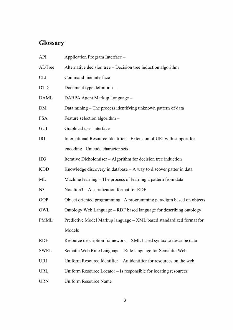
Glossary

API Application Program Interface –

ADTree Alternative decision tree – Decision tree induction algorithm

CLI Command line interface

DTD Document type definition –

DAML DARPA Agent Markup Language –

DM Data mining – The process identifying unknown pattern of data

FSA Feature selection algorithm –

GUI Graphical user interface

IRI International Resource Identifier – Extension of URI with support for

encoding Unicode character sets

ID3 Iterative Dicholomiser – Algorithm for decision tree induction

KDD Knowledge discovery in database – A way to discover patter in data

ML Machine learning – The process of learning a pattern from data

N3 Notation3 – A serialization format for RDF

OOP Object oriented programming –A programming paradigm based on objects

OWL Ontology Web Language – RDF based language for describing ontology

PMML Predictive Model Markup language – XML based standardized format for

Models

RDF Resource description framework – XML based syntax to describe data

SWRL Sematic Web Rule Language – Rule language for Semantic Web

URI Uniform Resource Identifier – An identifier for resources on the web

URL Uniform Resource Locator – Is responsible for locating resources

URN Uniform Resource Name

4

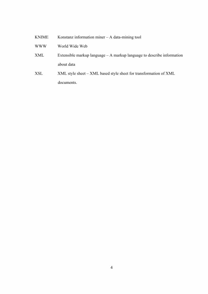
KNIME Konstanz information miner – A data-mining tool

WWW World Wide Web

XML Extensible markup language – A markup language to describe information

about data

XSL XML style sheet – XML based style sheet for transformation of XML

documents.

5

Figure

Figure 1. A learning machine predicting output based observation of the system [9] ....... 11Figure 2. KDD process [8] ................................................................................................... 13Figure 3. Decision tree structure .......................................................................................... 18Figure 4. Graphical representation of RDF [27] .................................................................. 29Figure 5. Protégé OWL integration [33] .............................................................................. 36Figure 6. Protégé OWL model class diagram [33] .............................................................. 37Figure 7. Classes for ontology management in OWL API [34] .......................................... 39Figure 8. Ontology building approach ................................................................................. 41Figure 9. The proposed architecture of dataset to SWRL .................................................... 43Figure 10. CSV dataset to ontology ..................................................................................... 45Figure 11. Sample WBCD dataset ....................................................................................... 47Figure 12. WBCD ontology ................................................................................................. 48Figure 13.Example Decision model induction workflow in KNIME .................................. 49Figure 14. Mapping PMML to Inductive Rule .................................................................... 52Figure 15. Mapping PMML to SWRL ................................................................................ 53Figure 16. WBCD SWRL rules ........................................................................................... 58

Table

Table 1. Simple example: weather problem ........................................................................ 12Table 2. Summary of Semantic Web architecture ............................................................... 25Table 3. SWRL atom types and examples [32] ................................................................... 34Table 4. Entity in ontology .................................................................................................. 54

6

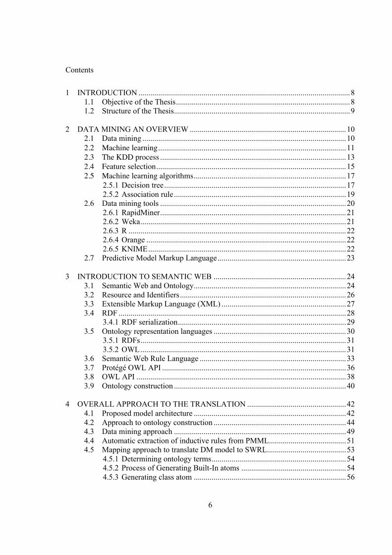
Contents

1 INTRODUCTION ........................................................................................................... 81.1 Objective of the Thesis ........................................................................................ 81.2 Structure of the Thesis ......................................................................................... 9

2 DATA MINING AN OVERVIEW ............................................................................... 102.1 Data mining ....................................................................................................... 102.2 Machine learning ............................................................................................... 112.3 The KDD process .............................................................................................. 132.4 Feature selection ................................................................................................ 152.5 Machine learning algorithms ............................................................................. 17

2.5.1Decision tree ............................................................................................ 172.5.2Association rule ....................................................................................... 19

2.6 Data mining tools .............................................................................................. 202.6.1RapidMiner .............................................................................................. 212.6.2Weka ........................................................................................................ 212.6.3R .............................................................................................................. 222.6.4Orange ..................................................................................................... 222.6.5KNIME .................................................................................................... 22

2.7 Predictive Model Markup Language ................................................................. 23

3 INTRODUCTION TO SEMANTIC WEB ................................................................... 243.1 Semantic Web and Ontology ............................................................................. 243.2 Resource and Identifiers .................................................................................... 263.3 Extensible Markup Language (XML) ............................................................... 273.4 RDF ................................................................................................................... 28

3.4.1RDF serialization ..................................................................................... 293.5 Ontology representation languages ................................................................... 30

3.5.1RDFs ........................................................................................................ 313.5.2OWL ........................................................................................................ 31

3.6 Semantic Web Rule Language .......................................................................... 333.7 Protégé OWL API ............................................................................................. 363.8 OWL API .......................................................................................................... 383.9 Ontology construction ....................................................................................... 40

4 OVERALL APPROACH TO THE TRANSLATION .................................................. 424.1 Proposed model architecture ............................................................................. 424.2 Approach to ontology construction ................................................................... 444.3 Data mining approach ....................................................................................... 494.4 Automatic extraction of inductive rules from PMML ....................................... 514.5 Mapping approach to translate DM model to SWRL ........................................ 53

4.5.1Determining ontology terms .................................................................... 544.5.2Process of Generating Built-In atoms ..................................................... 544.5.3Generating class atom ............................................................................. 56

7

4.5.4Generating individual property atom ...................................................... 564.5.5Generating data valued atom ................................................................... 574.5.6Use case: Breast cancer dataset ............................................................... 58

5 CONCLUSION .............................................................................................................. 60

6 REFERENCE: ............................................................................................................... 61

8

1 Introduction

Currently Semantic Web is widely adopted standard of knowledge representation.

Knowledge engineers are looking for sophisticated methods and automatic systems to dis-

cover and represent knowledge in Semantic Web form. Semantic Web is an addition to

current web. It presents an easier means to discover, reuse and share information [3]. Se-

mantic Web aims to link the distributed information on the web [3]; moreover, the infor-

mation in Semantic Web is represented in a way that humans and machines can understand

using semantics. There are different languages and standards presented for representing

information for Semantic Web. This includes ontologies, Resource Description Framework

(RDF) and Semantic Web Rule Language (SWRL).

Recent studies show that data mining techniques such as Decision Trees, Association

Rules etc. play an important role in capturing and representing knowledge in Semantic

Web standard [4][5]. Data mining techniques are integrated to the publicly available data

mining tools such as Rapid Miner, WEKA, R, Orange and KNIME for the purpose of data

mining. These data mining tools perform knowledge discovery to humans’ understandable

form. Some tools use Predictive Model Markup language (PMML) to represent knowledge

discovery. PMML represents the syntax of knowledge mining in a formalized way [2].

However, this mark-up language fails to address the representation of the semantics of the

discovered knowledge [1].

Therefore, study focus on close semantic gap in PMML. This thesis tries to research and

give solutions to translate PMML to Semantic Web standard (SWRL) using Semantic Web

technologies and data mining.

1.1 Objective of the Thesis

The objective of this thesis is to translate PMML based data mining model to Semantic

Web standard. In order to support the research, concepts related to machine learning and

Semantic Web standards are covered. The most important question of this thesis aims to

answer is:

9

1. How can we translate PMML based data mining model to Semantic Web standard?

Related supporting question is:

2. How to design automatic translation framework for translating PMML model to

Semantic Web standard?

1.2 Structure of the Thesis

The remaining chapters are organized as follows. In Chapter-2, we give a brief overview of

Data mining. We also present the data-mining concept with the relevant steps. Further-

more, features of the publicly available data-mining tools are elaborated. In Chapter-3, we

discuss the basic Semantic Web technology concepts, focusing on ontologies and SWRL.

In addition, we discuss technologies used for Semantic Web programming. In Chapter-4,

we present the proposed model to translate PMML to SWRL. We also provide examples

for each step in the translation process. Finally we conclude the paper in Chapter-5.

10

2 Data mining an overview

This chapter gives us the literature of background on Data Mining (DM) and Machine

Learning (ML). We explain the various steps of Knowledge Discovery in Database (KDD)

process. Furthermore, we discuss learning techniques that help to discover predictive

knowledge from data and existing open source DM tools.

2.1 Data mining

Data mining is the process of mining large dataset to identify unknown useful patterns. In

these days, data mining is a necessity because of the availability of abundant data [9]. In

DM, data is analyzed automatically or semi automatically using tools such as statistical

methods, mathematical models, and ML algorithms. According to Berry [10] the DM tasks

are: classification, prediction, estimation, affinity grouping, clustering and description

problems can stratify human problems. These concept as a whole is known as Knowledge

Discovery. DM tasks are divided into two categories: (a) prediction and (b) knowledge

discovery [9].

Knowledge discovery in database (KDD) is a collective name for the methods that help to

discover patterns in data [10]. Knowledge discovery comprises of all the necessary stages

from identifying initial target of mining to the extraction of nontrivial information from

data; data mining (DM) is part of that process. The three stages in KDD are data pre-

processing, data mining and data post-processing. The stages are further explained in the

section 2.3.

Predictive data mining (PDM) works in a similar fashion to a human handling data analysis

of small-scale dataset, although on a large-scale dataset PDM gets no constrains compared

to human. PDM learns from past knowledge and reuses this knowledge to solve new prob-

lems. Existing PDM tools are designed in a way to make human understand what the non-

trivial information is and show past the result from data mining procedure. As a result, the

tools can enable to discover similar hidden information using learning technique and also

build model for future use.

11

2.2 Machine Learning

Machine Learning (ML) is a branch of artificial intelligence and advanced form of pattern

recognition and computation-learning theory that is applied in a various computational

tasks where designing and programming of algorithms is impracticable [12]. Example of

ML includes spam filtering, fraud detection, and credit scoring. ML deals with the design

and programming of algorithms that enable machines to learn patterns on dataset. One of

the most applied ML task is known us inductive ML. Inductive ML is the process of pre-

dicting unknown input in relation with output, by observing the number of measurements

of input with outputs from a system. The learning process has three components as shown

in figure:

1. a random input vector X generator

2. a system that outputs Y for every vector X

3. a ML that predicts output Y1 by observing the system input-output samples

Figure1: A learning machine predicting output based observation of the

system [9]

Patterns learned in ML are expressed in two ways, a black box where the errors are unin-

telligible and as a transparent box where the structure of the pattern is reviled. Both ways

enable efficient prediction; however, the difference is we can examine the structure ex-

pressing the discovered pattern. Such pattern is known as structural because it enables us to

explain about the data. Most DM outputs are expressed in the form of rule [12]. Look at

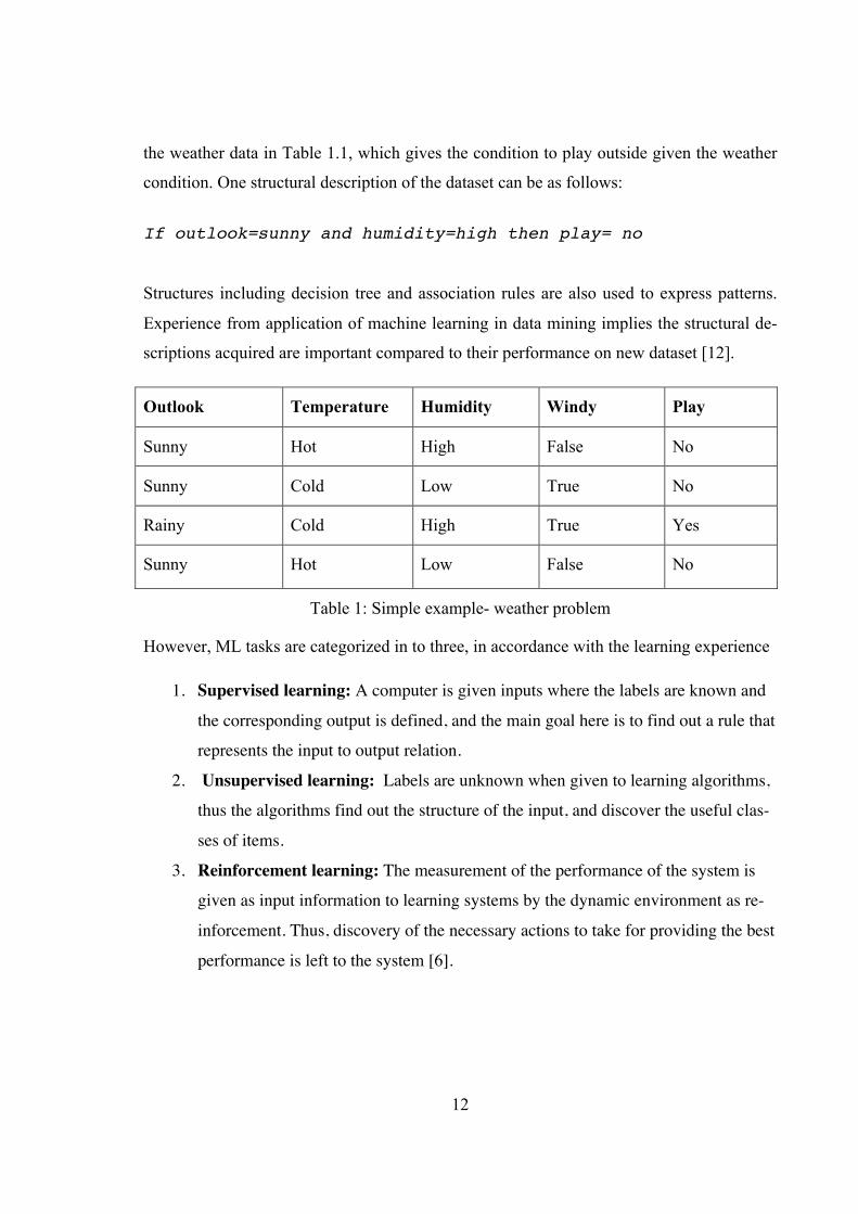
12

the weather data in Table 1.1, which gives the condition to play outside given the weather

condition. One structural description of the dataset can be as follows:

If outlook=sunny and humidity=high then play= no

Structures including decision tree and association rules are also used to express patterns.

Experience from application of machine learning in data mining implies the structural de-

scriptions acquired are important compared to their performance on new dataset [12].

Outlook Temperature Humidity Windy Play

Sunny Hot High False No

Sunny Cold Low True No

Rainy Cold High True Yes

Sunny Hot Low False No

Table 1: Simple example- weather problem

However, ML tasks are categorized in to three, in accordance with the learning experience

1. Supervised learning: A computer is given inputs where the labels are known and

the corresponding output is defined, and the main goal here is to find out a rule that

represents the input to output relation.

2. Unsupervised learning: Labels are unknown when given to learning algorithms,

thus the algorithms find out the structure of the input, and discover the useful clas-

ses of items.

3. Reinforcement learning: The measurement of the performance of the system is

given as input information to learning systems by the dynamic environment as re-

inforcement. Thus, discovery of the necessary actions to take for providing the best

performance is left to the system [6].

13

2.3 The KDD process

The KDD process begins with determining the end of the implementation of discovered

knowledge. So in turn this means that changes should be made in the applications domain

like offering many features to cell phone users for reduction in churning. This leads to the

halting of the loop and the results are then measured on new data repositories then the op-

eration is started again. The brief description of the nine-step KDD process is illustrated in

Figure 2.

Figure 2: KDD process [8]

1) Developing an understanding of the application domain

The goal of this step is to inform what must be done with the different decisions (i.e.

Transformation, Algorithms, Representation, etc.). When intending to create data mining

projects you need to understand and define the aim of the KDD from end-user viewpoint

and the environment in which the KDD will take place and understand the relevant prior

knowledge. In the continuation of the process revision and tuning of this step might occur.

After understanding the goal the pre-processing of data starts in the next three stages.

14

2) Creating a dataset on which discovery will be performed

After determining the goal the data for the KDD process on which discovery will be per-

formed must be determined. So in this step we must find what data is available; integrating

all the data for KDD into a single dataset. This process gives data mining learning and dis-

covering new patterns from the data it already has.

3) Pre-processing and clearing data

This stage gives you enhancement of data reliability and it clears the data such as handling

missing values and removing noise. It may involve using data mining algorithm in this

context for instance if an attribute has a missing data then we can use supervised data min-

ing algorithms to create a prediction model for the attribute and the missing value will be

replaced.

4) Data transformation

This stage makes you generate better data for data mining. You can use many methods

such as dimension reduction, feature selection and extraction, record sampling and attrib-

ute transformation which can be considered crucial for the success of the project. After

understanding the four steps the next four steps focus on the algorithmic aspects of the

project

5) Choosing the appropriate data mining task

This step deals with deciding the appropriate data mining technique that meets the aim of

DM i.e. classification, regression and clustering. Such decision relies on the aim of the

previous step. As mentioned in section 2.1 the DM task are categorized as description and

prediction depending on the outcome requirement.

6) Choosing the data mining algorithm

This stage makes us select a method for searching patterns. For instance, while considering

precision against understandability. Precision is better with neural networks while under-

standability is better with decision trees. When data mining algorithm faces a problem me-

ta-learning leads you to discover whether data mining algorithm will be successful or not.

15

7) Employing the data-mining algorithm

This step leads you to engage the algorithm so that the desired result will be obtained.

8) Evaluation

This stage gives the extracted patterns to be evaluated and interpreted. In this stage, we

focus on studying or evaluating the discovered model and the knowledge will be stored for

future use.

9) Using the discovered knowledge

In this stage, we incorporate the previously found knowledge into a system for further use.

The validity of the entire process is determined by this step. This stage is dynamic because

there are many changes for instance data structure, attribute may become unavailable, data

domain being modified.

2.4 Feature selection

Machine learning is used to generalize the functional relationship f( ) that relates input X=

{x1,x2…xi} with an output y, where xi are vector and yi are real numbers. In some condi-

tions the set of input features {x1,x2…xi} are not deterministic of the output, a subsetX = {X1,X2.......Xj} from the complete set determines the output, where j < i. If we are

provided with sufficient time, we can use the entire feature including redundant features to

provide the prediction of outputs.

In practice, redundant features result in increase in computation cost, predictor models with

big size and overfitting [20]. Therefore a method known us feature selection has been de-

veloped in the machine learning and statistics studies to overcome the problem of irrele-

vant features. An irrelevant feature is not important for data mining technique while the

relevant features are a necessity for the data mining technique [19].

The process of feature selection can be manual or automated. The meaning of relevance

motivates feature selection; however, the objective of the learning algorithms defines the

meaning of feature relevance. Isabelle and Andre’s article lists briefly the different defini-

tion of relevance in feature selection problem [19].

16

Furthermore, Louis and Jordi [20] listed three methods to follow for relevant feature selec-

tion:

1. “The subset with specified size that optimizes an evaluation measure”

2. “The subset of smaller size that satisfies a certain restriction on evaluation measure”

3. “The subset with the best commitment among the size and value the evaluation

measure” [20]

Moreover, detailed step to feature selection problem is explained in Isabelle and Andre’s

paper [19]. Feature selection algorithm (FSA) is highly dependent in the evaluation meas-

urement are utilized. The evaluation measure classifies the feature selection into three

methods: wrapper, filter and embedded method. In the filter method the features are select-

ed in the pre-processing stage, without directly enhancing the performance of data mining

technique. The method applies evaluation measure along with search method to find sub-

set of features. Applying exhaustive search is intractable for the entire initial set. As a re-

sult, the search strategies applied differs among the methods. Wrapper methods utilizes

predictive model to select feature subset. The method wraps the search on top of the select-

ed DM algorithm and scores feature subset depending on the learning output of data min-

ing technique and such method causes a computational complexity [20].

FSA is necessary to improve the learning speed, generalization capacity, reduce the noise

produced by irrelevant feature to avoid useless knowledge and provide simplified predictor

model of a given predictor. FSA enables to have better understanding of the process of

generated data. Furthermore, the simplified models minimize storage space and measure-

ment requirements. The FSA can be categorized into two types depending on the output:

1. Algorithms that provide feature which are ordered linearly

2. Algorithms that provide a subset from the original feature [19].

17

2.5 Machine learning algorithms

In this section we describe briefly the ML algorithms which express discovery of

knowledge using decision tree and association rule and structure of learning process which

are supervised ML and unsupervised ML respectively.

2.5.1 Decision tree

A brief description of the research on decision trees is provided in Murthy article [13]. The

article includes a guide on the utilization of decision tree for those who are practicing ML.

In this paper, we provide description of decision tree and DM techniques to acquire deci-

sion tree. Decision tree is a classification algorithm that represents DM model in a tree

structure that allows classifying of instances by rearranging them according to feature val-

ue.

Each node in decision tree denotes a test on the attributes with a possible extension deci-

sion tree for each possible result, while each branch denotes a value and each leaf denotes

a class. To classify an instance we start at the root node and test feature value accordingly

until we reach the last leaf in a branch. Figure-2 illustrates a decision tree example. For

beginning, the instance (f1= v2, f2= v3, f3=v5) is tested in nodes f1, f2, and f3 that finally

classifies to positive class with value ”+ve”.

Moreover, features that best classify the training set are at the top root of the tree. Various

studies have found out that not any best method is available to divide the training set, [14]

and thus comparison of the methods is necessary to identify the method that yields the best

result on a given data. However, trees with lesser leaves are preferable when two trees hav-

ing similar tests and prediction accuracy are compared. Over fitting training data is a phe-

nomenon where a decision tree learning yields a greater errand compared to another

learned result tested against training data, and lesser errand when tested against the entire

dataset. There are two known ways where decision tree learning techniques use to avoid

over fitting training data:

18

I. Before the training learning method fits the training data and learning procedure

should be stopped.

II. Other method mostly applied deals with pruning the induced on decision tree [15].

Figure 3: Decision tree structure

In the literature, various DM techniques are suggested for inducing decision tree from a

dataset. According to Quinlan, C4.5 classification algorithm is given preference [9]. In this

paper, we concentrate on Iterative Dichotomiser 3 (ID3), C4.5 and Alternating decision

tree (ADTree) algorithms as DM techniques for building decision tree structure model.

1) ID3 algorithm: ID3 is a supervised learning algorithm that learns decision tree by selec-

tion of best feature using information entropy [12]. The algorithm selects the best feature

to analyze at the root node and follows top-down approach to build decision tree. ID3 uses

nominal attributes with no unknown values when learning. Furthermore, in ID3 algorithm,

an information gain criterion is applied on a given features to select the best feature. Basi-

cally, the feature that best splits the training dataset has top gain information I(S) value at

the given node. The information gain is measured using the formulae below:

I(S) = − pi logi=1

m∑

2(p) ,

F1

F3

F2

F4

-VE +VE

-VE

V5

V3

V6

V4

V2 V1

19

Where I(S) is amount of information required to know label of class in the vector S. Pi is

the probability of given vector S classified to class.

2) C4.5 algorithm: C4.5 is a descendant of ID3 algorithm that generalizes classifiers in a

decision tree structure. The algorithm learns classifiers utilizing information criteria like-

wise in ID3. In contrast to ID3 algorithm, C4.5 differs by applying pruning method to over

fitting tree. Furthermore, C4.5 improves ability to utilize continuous data, data with miss-

ing value and features with different weights.

3) ADTree algorithm: ADTree originally introduced by Freund and Mason [16]; is boost-

ing technique that generalized decision tree. The algorithm constructs a combination of T

weighted decision trees where T indicates the number of boosting iteration. An ADTree

classifier generalized includes nodes that alternatively can have prediction condition, and

prediction nodes with a value expressed in numbers.

2.5.2 Association rule

Data mining based on association rule is used to find association and correlation in items

of large dataset [8]. An association rule shows the conditions of attribute values occurring

often within dataset. Association learning is applied in various DM problems including

predicting customer behaviors in business practice. For instance, rule could be found in a

bank transaction data from a supermarket that 90% of customers who buy product A also

buy product B. Association rules provide information in the form of a rule, and some met-

rics asses their quality, namely:

§ Support: the support of a rule is the frequency at which x and y are discovered to-

gether divided by the number of transactions and is calculated using the formulae-

Support = frq(x, y)n

§ Confidence: the confidence of an association rule( x ->y), quantifies X and Y fre-

quently occur together as a fraction of the number of times X occurs. Confidence

of a rule is calculated using the formulae-

20

confidence = frq(x, y)frq(x)

The most widely used Association Rules algorithm is the Apriori. Rakesh Agrawal and R.

Srikant developed this algorithm. This algorithm uses the search in breadth first search

(BFS) and a hash-tree structure for counting the sets of items efficiently. O algorithm gen-

erates a set of items of length k candidates, from a set of size items k-1. The candidate set

thus contains all common items of length k. Then, a scan is made over the database to de-

termine frequent sets of items from among the candidates [18].

2.6 Data mining tools

Throughout the years, advanced skills were required to understand or perform DM task

using DM tools. Nonetheless, currently available DM tools are designed to easily perform

data mining operations. As organizations are regularly consuming predictive model results

to decide their operation, the primary consumers of information are becoming business

users. Thus, a need is created for an easy to use DM tools for business users.

Software companies and DM communities are responding by developing a visual based

tool that not only provide intuitive graphical user interface but also hide mathematical

complexity. For instance, some tools provide support to assist users with the appropriate

model suggestion based on analysis of data available. These tools range from those, which

require expertise to those, which do not need any expertise to operate. In our study we

were interested in publicly available DM tools. A comparative study on open source DM

tools that includes the input/output support for each DM tool discussed in the following

section is provided in [21]. The detailed review with installation guide is referred in [22].

Notable open source DM tools include Rapid Miner1, WEKA, R2, Orange3, and KNI ME 4.

1 http://it.toolbox.com/wiki/index.php/RapidMiner 2 http://www.revolutionanalytics.com/what-r 3 http://orange.biolab.si/ 4 https//knime.org

21

2.6.1 RapidMiner

Rapid miner also previously known us YALE is a free DM tool based on Java; that is

widely used due to its cutting edge technology and different functionalities. RapidMiner

offers intuitive graphical user interface (GUI) or command line interface (CLI) versions for

users to preform different DM tasks. Processes are the heart of RapidMiner. Processes in-

clude visual components that represent each operator. Operator defines DM technique im-

plementation and data sources. The tool allows performing drag and dropping operation on

operators and to connect inputs with output to build dataflow, and also provide automatic

process construction facility whereby processes are constructed based on DM goal. Rapid

miner provides support for most of DM learners including decision tree and Association

rule. However, the tool has limited support for advanced machine learning algorithm (e.g.,

randomized trees, inductive logic learning algorithms) [22].

2.6.2 Weka

Weka is an open-source DM tool built with Java for non-commercial use. Weka was most

preferable due to user friendly GUI and providing numerous DM algorithm implementa-

tion. However, when compared with R and RapidMiner the algorithm implementation in

Weka requires more resource. Thus, R and RapidMiner are famous in academic and com-

mercial use.

Weka offers four options for DM task: CLI, Experimenter, Explorer, and Knowledge flow.

The explorer option is given preference as it provides tools to define data source, data

preparation, machine learning technique, and visualization. The experimenter option al-

lows comparing different machine learning algorithms performance on a given dataset. The

knowledge flow operates in the same manner as RapidMiner's operator of function. Weka

supports various procedure model evaluators and measurements; however, provides limited

options for data visualization and surveying. Furthermore, Weka provides more support

classification (e.g., decision tree, association rule) and regression tasks. Weka supports

PMML as input format.

22

2.6.3 R

R is an open-source tool based on S programming language, that’s not only preferable by

statisticians, but also used for DM task. R is an interpreted language that is utilized for ma-

trix based calculations and has a close performance to commercial available software

(MatLab). In particular, data exploration, data visualization and data modeling task options

are provided in R easy to use programming environment. Although R based machine-

learning algorithm perform fast, the language is difficult to learn. Thus, a user friendly

GUI called Rattle is used by the DM community.

2.6.4 Orange

Orange is a Python-based tool that provides visual programming interface for data analy-

sis. The user interface of Orange is based on Qt framework. The visual interface provides

support for functionalities including visualization, regression, evaluation, unsupervised

learning, association, and data preparation. Furthermore, Orange supports comparison of

learning procedures. Functionality is expressed in different widgets and a description of

the functionalities is provided within the interface. The interface allows performing pro-

gramming by simply placing widgets on canvas and connecting individual inputs and out-

puts.

2.6.5 KNIME

KNIME (Konstanz Information Miner) is an open-source DM tool that is based on the

nodal task. The tool follows a visual based paradigm where the components are placed on a

canvas to visually program a DM task. The components are known as nodes and more than

1000 nodes and extension nodes are presented on a fresh installation of the software. The

tool provides integration to the Weka and R with the help of extensions. Furthermore,

KNIME follows a modular approach that allows documenting and storing the procedure of

analysis that finally ensures results to be available to the end user. The tool has strong vis-

ual based programming paradigm. KNIME supports PMML as input and output format.

23

2.7 Predictive Model Markup Language

The Predictive Model Markup Language (PMML) is a standard for storing DM models. It

is based on XML and allows sharing models between applications thereby facilitating in-

teroperability. Currently the major suppliers of ‘Data Mining solutions’5 already adopted

PMML. The PMML provides applications independent method of defining models so that

property rights and incompatibilities are no longer barriers in the exchange of models be-

tween applications. Thus, PMML enables users to develop models with in an application

and use another application to view, analyze and make other tasks using the model created.

Since the PMML uses the standard XML, its specification is in the form of XML schema,

shown below.

<PMML xmlns="http://www.dmg.org/PMML-4_1" version="4.1"> <Header copyright="KNIME"> <Application name="KNIME" version="2.8.0"/> </Header> <DataDictionary numberOfFields="5"> <DataField name="sepal_length" optype="continuous" dataType="double"> <Interval closure="closedClosed" leftMargin="4.3" rightMargin="7.9"/> </DataField> .... </DataDictionary> <TreeMod-el modelName="DecisionTree" functionName="classification" splitCharacteristic="binarySplit" missingValueStrategy="lastPrediction"noTrueChildStrategy="returnNullPrediction"> <MiningSchema> <MiningField name="sepal_length" invalidValueTreatment="asIs"/> <MiningField name="sepal_width" invalidValueTreatment="asIs"/> <MiningField name="petal_length" invalidValueTreatment="asIs"/> <MiningField name="petal_width" invalidValueTreatment="asIs"/> <Mining-Field name="class" invalidValueTreatment="asIs" usageType="predicted"/> </MiningSchema> <Node id="0" score="Iris-setosa" recordCount="150.0"> <True/> <ScoreDistribution value="Iris-setosa" recordCount="50.0"/> <ScoreDistribution value="Iris-versicolor" recordCount="50.0"/> <ScoreDistribution value="Iris-virginica" recordCount="50.0"/> . . . </Node> </TreeModel> </PMML>

Listing 1: Tree model in PMML format

5 http://www.dmt.org/DataMiningGroup-PMMLPowered-product.html

24

3 Introduction to Semantic Web

In this chapter we present the brief definition of Semantic Web6 and the standardized tech-

nologies that are widely used to present Semantic Web data. We give brief introduction

about RDF, RDF schema, SWRL and OWL. Semantic Web is a vision that was proposed

by Sir Tim Berners-Lee that “enables machines to interpret and understand documents in

meaningful manner” [3].

3.1 Semantic Web and Ontology

Over the year’s huge amount of data is presented on World Wide Web (WWW) with the

help of Web sites. Most of the web contents are designed in a way for humans to under-

stand but not for machines. Computers can process web pages for layout and route. For

instance, machine can present a document following a link presented in another document.

However, machines are not able to “understand” the unstructured information residing in

documents [3]. As search engines, agents and other machines use of the WWW is increas-

ing, machine understandability of the content of a page is given importance.

Sematic web is a vision for next-generation web, which is used by humans and machines.

Semantic Web is proposed to extend the current WWW where meaningful content of the

Web page is structured. As a result, agents or machine can perform a complicated task for

humans and this enables implementation of next generation application and intelligent ser-

vices. Currently, integration of Semantic Web to the current Web is in progress [3]. As a

result, the integration assures new functionalities in future as machine capability to process

and “understand” semantic documents grows.

Moreover, one problem in the current web is uncertainty and accuracy of information in

documents. The problem lies in the mere idea that anyone can publish information and

opinions. However, Semantic Web is intended to increase the trust of information pub-

lished.

6 http://semanticweb.org

25

Sir Tim Berners-Lee has constituted Semantic Web into seven-layered architecture as

summarized in table-2. In lower level of the architecture, we have basic technologies such

as XML and XML-schema. The higher level includes technologies that are expressive and

powerful languages, and individual layer is built on top of lower layer.

Low

High

Layers Name Description

Layer 1 Unicode and URI Unicode is responsible for resource

encoding and URI for resource

identification

Layer 2 XML+NS+XML-

schema

Represents structure and content of data.

XML schema presents the applicable

tags and structure definition.

Layer 3 RDF7+RDF

schema8

Used to define semantic web resource

and type. The RDF schemas built on top

of RDF enable to define relation

between resources.

Layer 4 Ontology vocabulary Used to specify resource relationship

and type

Layer 5 Logic Responsible for defining logic and

reasoning

Layer 6 Proof Used to verify defined statement with

logic

Layer 7 Trust Establish trust among users

Table 2: Summary of Semantic Web architecture

7 http://www.w3.org/RDF/ 8 http://www.w3.org/TR/rdf-schema/

L

26

XML, Ontology and RDF(s) are the core of the Semantic Web architecture. Semantic Web

is formed with the three core technologies. The technologies present ways to semantically

describe knowledge and information to provide semantic knowledge exchange and reuse.

Ontology is an explicit representation that specifies shared conceptualization of a specific

domain that is machine processable and human readable. Conceptualization means model

of phenomena with explicit definition of relevant concepts of a phenomena. Explicit refers

to restriction and types of concepts are defined explicitly. Thus, machines are able to inter-

pret information with the meaning or semantics. Shared conceptualization defines that the

concept described is recognized by the group not only individuals. Basically, ontology is

defined using terms where the conceptual entities (class, property, restrictions) are de-

scribed in human readable format [26].

3.2 Resource and Identifiers

Uniform Resource Identifier (URI) is used for the identification of resources in the web. In

URI resource refers to “things” that have identity and are network-retrievable, such as im-

ages, documents or services. Generally a resource is anything in the world that has identity;

for instance, books, institutions and human beings. Every resource in the web is assigned a

unique URI to enable easy access and retrieval of information. The detail specification of

the URI is defined in RFC 1630. [23]

The URI is formed with combination of symbols and characters. Although the access

method used for the resources varies, uniformity in URI delivers various kinds of resource

identifiers to be used in similar context. Furthermore, uniformity enables uniform semantic

definition of mutual agreements of different resource identifiers and also easies the intro-

duction of a new kind of identifier without affecting the way current existing identifiers

operate. URI can be further categorized into a Uniform Resource Locator (URL) and Uni-

form Resource Name (URN).

URL is responsible for locating or finding of available resources via Internet. The URL

follows a specified syntax and semantics for representing location and network retrieval of

27

the available resources. The specification of URL is based on the RFC 1738 [24], which is

introduced following the specification in RFC 1630. The following examples of URL with

various kind of scheme:

• http://uci.org

• ftp://ftp.ic.se/rfc/rfc.txt<

• gopher://spinaltap.micro.umn.edu/00/Weather/California/LosAngles

URN refers to URI implementing URN schema to uniquely identify resource. The identifi-

er is derived from a group of namespace, a specific name structure and procedure. The

URN has no knowledge of the availability of the resource. An example of URN is:

• tel:+358440933422.

An international resource identifier (IRI) is an extension of URI that delivers support for

encoding of Unicode character sets. The IRI is specified in RFC 3987 [25]. The IRI speci-

fication states mechanisms to map IRI to URI and also provides additional protocol ele-

ment definition. A general definition of IRI has the following form:

IRI = scheme “:” ihier-part[ “?” iquery] [“#” ifragment],

Where the “scheme” refers the IRI type (http, ftp, gopher), and the rest of the portions state

the name of the resource. The following examples of the IRI are:

• http://uci.org

• ftp://ftp.ic.se/rfc/rfc.txt

• urn:isbn:122-8234924742

3.3 Extensible Markup Language (XML)

XML is a Markup language that is used to represent a structure of information on the web.

XML is designed to meet the need for publishing large amount of electronic documents.

XML is actively used mainly for exchange of information on the Web. XML enables users

to create a tag to provide annotation of web pages or section of web content. A program

28

can be used to automatically create the tags on xml documents but the program writer is

required to have a prior knowledge of tag meanings and context. Generally, a document

type definition (DTD) and XML schema define constraints on which tags are applicable

and how they are arranged in a document. In general, XML is flexible to add structure to a

document, but lacks definition of the semantics of the structure. A structure language RDF

is created for Semantic Web to enable defining semantic information.

3.4 RDF

RDF is a W3C recommendation method that allows representing information on the web

using XML based syntax. RDF evolved from W3C Semantic Web activity that studied to

find out a language for machine processable data exchange [26]. The main purpose of RDF

is to define a data model for describing data to be processed not only by humans, but also

web application and agents on the web. Thus, it allows any domain data to have meaning

and be processed by automation. The description of RDF also defines the relation of re-

sources by using defined properties. Recent studies have provided the benefits of RDF, and

one of the benefits is defining meta-data for information on the web.

The web information described by RDF is stored online or offline in the form of state-

ments. Statements contain a combination of resources, property and statements.

• Resource:Aresourceisanythingthatisidentifiable.Awebpageorsectionofweb

pagecanberesource.URIareusedtouniquelyidentifyresources(Seesection

3.2).

• Property:Apropertyisusedtouniquelydefinetherelation,attributeandcharac-

terofaresource,suchus‘writtenBy’and‘homePage’.Thepropertiesareidenti-

fiedusingURIs.

• Statement:Astatementdefinedspecificresourceincombinationwithaproperty

andpropertyvalue,wherepropertyvaluecanbeliteralorresource.

29

Figure 4: Graphical representation of RDF [27]

RDF defines standard syntax to describe basic models that are object, property and value.

Subject-predicate-object triplets describe each object.

The subject with label http://jyu.fi/paper/semanticWebAnddataMining

identifies the object http://users.jyu.fi/~edris in question that is a resource.

But can also be literal. The predicate with label http://jyu.fi/term/writtenBy

defines the relation between subject and object. The object represents a resource or literal

with value such us number and strings. In graphical format the relation can be represented

as shown in Figure-4. RDF graph representation is exchanged and stored using various

syntax and serialization formats. These are RDF/XML, N3 and N-Triples. In this section,

we provide basic introduction to the serialization methods. In depth explanation of the

formats is provided in the book “PRACTICAL RDF” [26].

3.4.1 RDF serialization

The RDF/XML is serialization method for RDF data that is based on XML syntax. Basi-

cally the statements from graph representation are mapped to a XML standard in

RDF/XML. The URIs from graph model is encoded using QNames or as attribute of an

xml element.

Notation3 (N3) is well known serialization format for RDF documents. N3 is an extension

to RDF by adding more functionality to express, add formulae and more. However, N3

isn’t accepted w3c recommendation [26]. In this work, we use N3 for serialization of RDF

hXp://jyu.fi/paper/seman[cWebAnddataMini

ng

hX://jyu.fi/term/wriXenBy

hXp://users.jyu.fi/~edris

30

documents. The syntax structure for N3 is “subject predicate object”. For

instance, the RDF graph in figure-4 is represented in N3 as follows:

<http://jyu.fi/paper/semanticWebAnddataMining>

<http://jyu.fi/term/writtenBy> <http://users.jyu.fi/edris>.

A QName, that are defined XML names in a document are used to simplify the N3 encod-

ing. Generally, QName includes a prefix that represents a namespace URI followed by a

colon and a local name. For instance,

Prefix URI associated with prefix

jy http://jyu.fi/paper/

jyu http://jyu.fi/term/

j http://users.jyu.fi/

Then the QName for the RDF graph in Figure-4 is as follows:

<jy:semanticWebAnddataMining> jyu:writtenBy <j:edris>.

N-Triples is a subset of N3 that follows the same specification format for encoding triplets.

Basically N-Triples is simplified from N3. Each line contains either a statement or a com-

ment in N-triples, where the statements provide the subject-predicate-object triplets. Fur-

thermore, blank nodes are encoded with the notation “_:” followed by a string.

3.5 Ontology representation languages

RDF languages are used to represent structure of part of certain data. The structure defin-

ing description together with the data provides knowledge. RDFs and OWL technologies

are presented for defining structure of ontologies. RDFS is a language that is less expres-

sive and powerful though used to describe statement about resource. Unlike RDFs, OWL is

more expressive language that describes statements of individual and properties.

31

3.5.1 RDFs

RDFs or RDF vocabulary description language is a schema language that enables to en-

code application-specific properties for classes, concepts of classes, sub-classes and sub-

properties. RDFS expressive power is to allow describing a combination of unique re-

sources to extend RDF [27]. Statements in RDF data model are interpreted using the defi-

nitions in RDF schema. The modeling primitives in RDFs describe resources and relation

among resources are as follows:

• Classes in RDFs are similar to particular classes in Object-Oriented Programming

(OOP). OOP properties are defined as an attribute and are attached to a specific

class, while RDF classes are particularly defined at a global level and attached to

classes to define class properties. Classes are formed with combination of

rdfs:Resource, rdfs:Property and rdfs:Class. Everything defined in RDF descrip-

tion is an instance of rdfs:Resource. rdfs:Property is the class for all properties that

describe characteristics of instance of rdfs:Resource. All concepts are described us-

ing rdfs:Class.

• Properties are rdf:type, rdfs:subPropertyOf, rdfs:subClassOf. The relation among a

resource and class is modeled using rdf:type. Furthermore, relation of hierarchy of

class is defined with rdfs:subClassOf . Likewise, rdfs:subPropertyOf is used to

model hierarchy of property.

• Constraints enable RDF to model restriction on properties and classes. The main

constraints are rdfs:constraintResource, rdfs:constrainProperty, rdfs:range, and

rdfs:domain.[28]

3.5.2 OWL

In 1997, Ontology Inference Layer (OIL) was released. It followed the XML schema and

RDF for encoding ontology. Then in 2000, an American research group released DARPA

agent markup language (DAML) that followed the standardization of W3C. In the follow-

ing year DAML+OIL was released. DAML+OIL encoding was based on the standards of

RDF and RDF schema. Further, DAML+OIL was the foundation for the ontology research

activity of W3C [27].

32

The ontology research group from W3C released the first version OWL in 2004 [28].

OWL is a language for encoding web ontologies and additional knowledge bases. The on-

tology is composed of classes, individuals and properties that encode knowledge from the

real world. The ontology is described using RDF and embedded in Sematic Web docu-

ments to allow knowledge reuse by referencing it to other documents. In 2009, the revised

version OWL29 was released. OWL2 has advanced reasoning capability on ontologies than

OWL [30]. OWL2 is used to describe knowledge about things and relation between things

for a specific domain. Furthermore, Ontologies from a given domain are described using a

combination of statements in OWL2. These statements are terminologies, assertion state-

ments of specific domain. Some of the features of OWL2 are as follows:

• OWL2 is a declarative language not a programming language [30]. There are nu-

merous tools that are designed to process and infer knowledge.

• OWL2 is not schema language to conform syntax. OWL2 doesn’t define con-

straints. As the Semantic Web and RDF follows open world assumption the prob-

lem with syntax conformation exists. Thus, when missing information from a given

data, one can’t conform the information’s inexistence.

• OWL 2 is not a database. Database schemas follow a close world assumption, and

absence means inexistence; while in OWL2 absence means unknown.

• OWL2 provides features to describe characteristics of properties. For instance, we

can define a property to be symmetric of another. Further, properties can be con-

figured to be transitive, symmetric, functional and inverse of another property. [30]

OWL2 provides three basic categories to model data. These are entities that represent real

world object, Axioms that describe statement of ontology and expressions that are defined

by a structure to describe complex representation in the domain. Basically, Axioms are

statements that are evaluated to a Boolean value on a certain condition. For instance, the

statement “Every mammal is male”.

Entities describe real world objects, relation and categories with individual, properties and

classes respectively, and are identified with IRI (see Section 3.2). Properties describe rela- 9 http://www.w3.org/TR/owl2-overview

33

tions among objects. Properties are further categorized into object, data type and annota-

tion properties:

• Data type property defines the characteristics of a class. For instance, height of a

person defines data type property.

• Annotation properties are used to annotate ontologies.

• Object properties define relation among object.

3.6 Semantic Web Rule Language

The Semantic Web Rule Language (SWRL) is rule language that can be used in Semantic

Web. The specification for SWRL was submitted in May 2004 to World Wide Web con-

sortium [31]. Although the rule language is not a recommendation language, it is part of

the member submission to World Wide Web consortium. SWRL is rule language that ex-

tends OWL to express logic and rules. SWRL rule is described using concepts in OWL to

reason on ontology individuals. The rule language has antecedent and consequent to state

rules and can be described in “human readable” 10 syntax. For this work, we will use the

defined “human readable” syntax.

antecedent⎯→⎯ consequent .

The antecedent states conditions that need to be fulfilled for the consequent to be true. Fur-

thermore, as a convention variables are expressed using question mark prefix such as (?x).

Antecedent and consequent are written as combination of atoms as ( c1∧c2.........∧cn ).

SWRL submission states that, both antecedent and consequent have no atom to valid [45].

The member submission states that antecedent having no atom is asserted to be true and

the statements in the consequent are considered to be true. In the contrary, if a consequent

has no atom then the rule is asserted to be false. This indicates that neither the consequent

10The syntax used for expressing SWRL rule in this work follows the SWRL syntax used in Proté-

gé SWRL Tab. The syntax is not part of the submission to World Wide Web consortium.

34

nor the antecedent can be fulfilled by any ontology. The case where the antecedent match-

es elements in the ontology is considered to make the ontology contain inconsistency.

SWRL enables to do deductive reasoning and infer new knowledge from existing ontolo-

gy. For instance, a SWRL rule asserting that a “person with parent and parent sister has

aunt” can be defined using concepts ‘person’, ‘parent’, ‘sister’ and ‘aunt’. The rule in

SWRL would be:

Person(?x) ∧hasParent(?x,?y) ∧ hasSister(?y,?z) ⎯→⎯ hasAunt(?x,?z)

Basically, the concept person is expressed using an OWL class called Person. The sister

and parent relationships are described using OWL properties hasParent, hasSister

and hasAunt are defined as characteristics of Person class. The execution of the rule in-

fers a person x having a parent y that has a sister z to have z as an aunt.

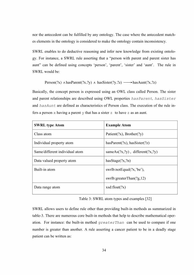
SWRL type Atom Example Atom

Class atom Patient(?x), Brother(?y)

Individual property atom hasParent(?x), hasSister(?z)

Same/different individual atom sameAs(?x,?y) , different(?x,?y)

Data valued property atom hasStage(?x,?n)

Built-in atom swrlb:notEqual(?x,’be’),

swrlb:greaterThan(?g,12)

Data range atom xsd:float(?x)

Table 3: SWRL atom types and examples [32]

SWRL allows users to define rule other than providing built-in methods as summarized in

table-3. There are numerous core built-in methods that help to describe mathematical oper-

ation. For instance: the built-in method greaterThan can be used to compare if one

number is greater than another. A rule asserting a cancer patient to be in a deadly stage

patient can be written as:

35

Patient(?x) ∧ hasCancer(?x, true)∧ hasStage(?x,?y) ∧swrlb:greaterThan(?y,2) → DeadlyStagePatient(?x)

Executing this rule can stratify cancer Patient, which hasCancer property value true and

hasStage property value greater than 2 as a member of DeadlyStagePatient class. The class

atom refers to a class existing in the ontology. The class atom is followed with a reference

to name individual or variable. If the class atom is in the consequent, the class must have

the variable or named individual for the rule to evaluate to be true. If the class atom is in

the antecedent, the class must have the variable or named individual as an instance for the

rule to evaluate to true.

Moreover, the data range atom contains defined variable followed with individual datatype

or multiple datatypes. If the data range atom exists in the consequent, the variable attached

to the atom must have the defined datatype for the rule to evaluate to true. If the data range

atom is defined in the antecedent, the variable or value should be the defined datatype to

evaluate the rule to true. For instance, the data range atom example in table 3 asserts that

variable x be only a float datatype.

The individual property atom defines relation between two specific individuals or variables

using the object property. If the individual property is in antecedent then the triplet should

exist for the atom to evaluate to true. If the individual property is in the consequent, the

triplet will be asserted. All classes and properties expressed in SWRL rule have to pre-exist

in the ontology where the SWRL rule is embedded.

The same individual atom is used for asserting if two specific variable or individuals are

equal. This declaration resembles the owl:sameAs , that is used between individuals and

variables. The different individual atom asserts if two specific variables or individuals are

different. This deceleration resembles the owl:differentFrom.

36

3.7 Protégé OWL API

Protégé11 is an easy to use and configurable tool for the development of ontology-based

application. The architecture of the tool enables to easily integrate new plugins, widgets or

handle new task in a given model. The Protégé-OWL editor provides various editing facili-

ties for ontology development. Developers are allowed to utilize the different components

in Protégé tab to design ontology and save the ontologies for further reuse.

The protégé-OWL API12 is an open source Java based tool that enables to perform ontolo-

gy management tasks; such as editing ontology data model, querying, and also reasoning

using the Description Logic engine. In addition, the API is utilized for the implementation

of graphical user interfaces. Likewise, Jena 13 is a Java based API, which is used with RDF

and OWL. Jena provides functionalities that enable to parse query and also visualize on-

tology. The older version of Protégé OWL API (3.4) and also the one before that provide

integration of Jena API as shown in Figure 5. The Protégé-OWL parser uses the Jena par-

ser. Further, in Protégé-OWL the implementation of validation and processing of datatype

and various other functionalities are based on Jena.

Figure 5: Protégé OWL integration [33]

11 http://protege.stanford.edu/ 12 http://protege.stanford.edu/plugins/owl/api/ 13 http://jena.sourceforge.net/

37

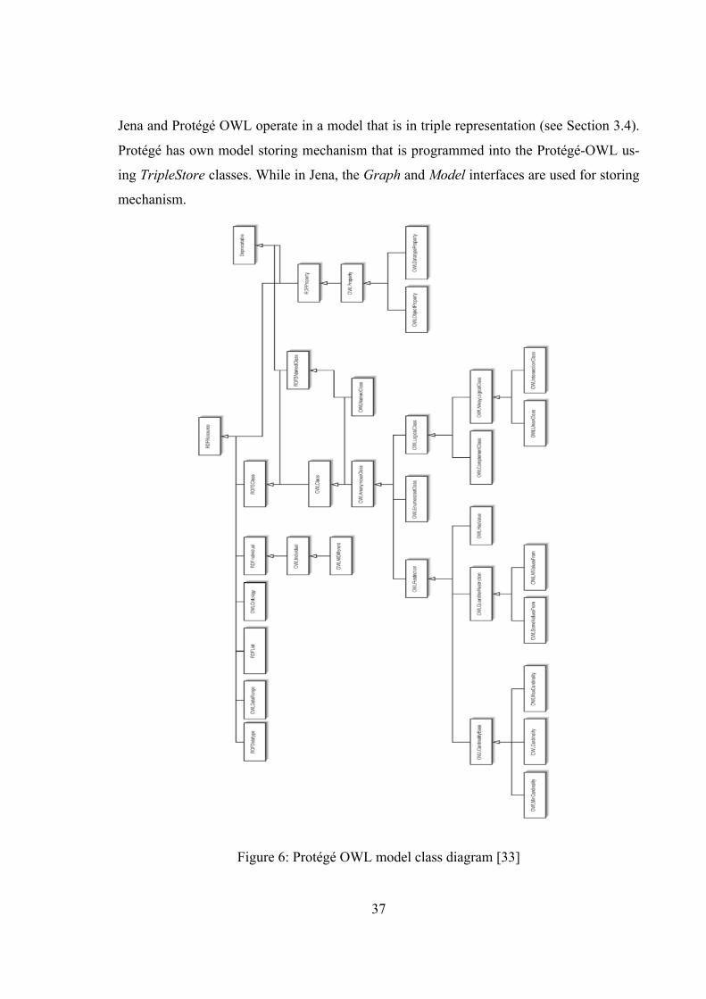
Jena and Protégé OWL operate in a model that is in triple representation (see Section 3.4).

Protégé has own model storing mechanism that is programmed into the Protégé-OWL us-

ing TripleStore classes. While in Jena, the Graph and Model interfaces are used for storing

mechanism.

Figure 6: Protégé OWL model class diagram [33]

38

The Protégé-OWL model has hierarchical structure for the representation of interfaces. A

class diagram model representation of the interfaces is shown above in Figure-6. The sub

interfaces for classes, properties and individuals are derived from the base interface

RDFResource. Furthermore, the classes are divided into named classes and anonymous

classes. The named classes provide an interface to create individuals, while the logical re-

strictions of named classes are described using anonymous classes.

3.8 OWL API

The approach described in chapter-5 is implemented with OWL API14 (4.2). The OWL

API is an open source project based on Java for working with OWL2. The high level API

provides OWL ontology management functionality. Furthermore, the major features of the

API includes an abstraction based on axioms, reasoner support, validator that works with

OWL2 profile and provides support for parser and serialization of the different syntax’s

available. OWL API has been used to implement various projects, including Protégé 4,

SWOOP, the NeOn Toolkit 15, OWLSight16, OntoTrack, and the Pellet17 reasoner. The

OWL API provides interfaces that allow developers to easily program at suitable abstrac-

tion level without handling issues such us, serialization and parsing a data structure.

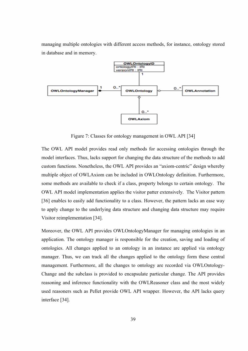
Moreover, the design of OWL API is based on the OWL 2 specification [35]. Ontology is

expressed as a set of axioms and annotation as shown in Figure-7. Similarly to Protégé-

OWL, in OWL API interfaces are represented in a hierarchical structure. The names and

the hierarchy structure for axioms, entities and classes closely resemble OWL2 structural

specification and provide a high level definition of OWL2 integration to the design of the

OWL API. OWL API provides support for loading and saving of ontology in a variety of

syntax. In contrast to Protégé 3.x API, the OWL API follows no concrete syntax or model

to represent the interfaces or models [35]. The OWLOntology interface provides methods

to access annotation and axioms for a particular class. Furthermore, the interface allows

14 http://owlapi.sourceforge.net 15 http://theneon-toolkit.org/ 16 http://pellet.owldl.com/ontology-browser/ 17 http://clarkparsia.com/pellet

39

managing multiple ontologies with different access methods, for instance, ontology stored

in database and in memory.

Figure 7: Classes for ontology management in OWL API [34]

The OWL API model provides read only methods for accessing ontologies through the

model interfaces. Thus, lacks support for changing the data structure of the methods to add

custom functions. Nonetheless, the OWL API provides an “axiom-centric” design whereby

multiple object of OWLAxiom can be included in OWLOntology definition. Furthermore,

some methods are available to check if a class, property belongs to certain ontology. The

OWL API model implementation applies the visitor patter extensively. The Visitor pattern

[36] enables to easily add functionality to a class. However, the pattern lacks an ease way

to apply change to the underlying data structure and changing data structure may require

Visitor reimplementation [34].

Moreover, the OWL API provides OWLOntologyManager for managing ontologies in an

application. The ontology manager is responsible for the creation, saving and loading of

ontologies. All changes applied to an ontology in an instance are applied via ontology

manager. Thus, we can track all the changes applied to the ontology form these central

management. Furthermore, all the changes to ontology are recorded via OWLOntology-

Change and the subclass is provided to encapsulate particular change. The API provides

reasoning and inference functionality with the OWLReasoner class and the most widely

used reasoners such as Pellet provide OWL API wrapper. However, the API lacks query

interface [34].

40

3.9 Ontology construction

Ontology construction comprises series of steps:

• Design: Describes the domain and goal of the ontology

• Develop: Defines whether ontology construction starts from scratch or we reuse

existing ontology.

• Integrate: Develop integration of the new ontology on existing ontology.

• Validate: Verify the completeness of ontology using automated tools and consult

experts to validate the constructed ontology consistency

• Iterate: Repeat the steps and apply expert comments about ontology.

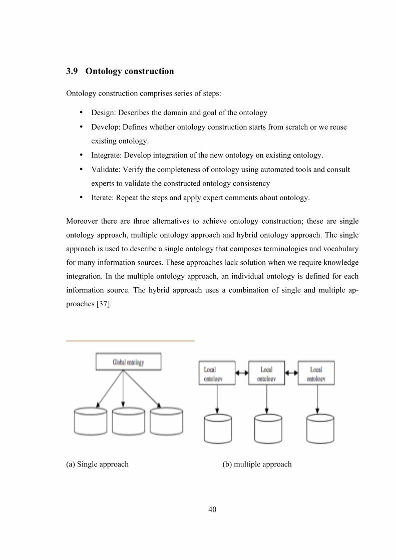
Moreover there are three alternatives to achieve ontology construction; these are single

ontology approach, multiple ontology approach and hybrid ontology approach. The single

approach is used to describe a single ontology that composes terminologies and vocabulary

for many information sources. These approaches lack solution when we require knowledge

integration. In the multiple ontology approach, an individual ontology is defined for each

information source. The hybrid approach uses a combination of single and multiple ap-

proaches [37].

(a) Single approach (b) multiple approach

41

(c) Hybrid approach

Figure 8: Ontology building approach

Generally, there are three ways followed to the ontology construction; manual, semi-

automatic and fully automatic. The manual construction involves full human intervention

for the construction process. Semi-automatic construction requires human involvement

during the constriction process. While in automatic construction the whole process of con-

struction is handled by computer system [38].

42

4 Overall approach to the translation

This chapter presents the approach learned from this research to translate PMML data min-

ing knowledge from dataset to ontology based rule language (SWRL). Section 4.1 de-

scribes the general architecture of software artifact built for the experiment. Section 4.2

provides general aspect of the domain ontology construction. Section 4.3 gives information

on the data mining approach. Section 4.4 details the overall approach to retrieve individual

rules from a data-mining model. Section 4.5 presents the mapping approach followed to

translate inductive rule in PMML file to SWRL atom.

4.1 Proposed model architecture

The proposed approach in this paper is to translate PMML rule-based knowledge from a

tabular dataset to Semantic Web standard. The rules extraction system requires dataset,

DM knowledge and domain ontology as an input. The datasets are stored in CSV files and

describe a particular domain. OWL ontology is used to describe the temporary ontology

provided in the CSV file. In addition to the temporary ontology, a DM model is prepared

from the dataset in the form of PMML (see Section 2.7) and used in the translation process.

The basic architecture of the system18 is illustrated in Figure 9. It consists of 5 main units:

ontology generation, rule transformation, SWRL translation, alignment module and Swing

UI.

The ontology generation unit is responsible for automatic generation of temporary domain

ontology from tabular data (see Section 3.8 and Section 4.2). The datasets used to test on-

tology construction are gathered from UCI repository [40]. The UCI19 repository is ma-

chine-learning repository that provides several public datasets for machine-learning com-

munity.

18 https://github.com/amanEdris/sematicDM 19 http://archives.ics.uci.edu/ml

43

The rule transformation unit is responsible for transforming PMML based DM model de-

veloped from a particular dataset to ‘Rule XML’20 by applying XSL style sheet. The XSL

style sheets are prepared for individual PMML models (decision tree, association rule)

available to ease the transformation process.

The SWRL translation unit models are necessary functionalities to transform XML based

rules into ontology-based rule (SWRL). Basically, the SWRL translation unit works to-

gether with rule transformation unit to achieve full translation of PMML model to Seman-

tic Web standard.

Figure 9: The proposed architecture of dataset to SWRL

The alignment unit is part of an external service that is responsible for mapping entities in

temporary ontology to domain ontology entities. The domain ontology is an ontology de-

signed by expert knowledge engineers in the domain. Moreover, the alignment module is a

potential part of future work. Finally, the Swing UI unit is responsible for providing basic

interface between a user and the system.

20 Rule XML- is XML based ”if-then” rule extracted from a data-mining model.

44

4.2 Approach to ontology construction

In this research, the main objective of domain ontology construction is to convert a CSV

data into OWL ontology from flat presentation of data to semantic representation. Here we

consider the definition and understanding of CSV file to describe the approach adopted

from [41].

CSV files are standard formats to store data from same domain and exchange between ap-

plications. Various enterprise applications provide support for such files. Data from rela-

tional databases are stored in CSV format after explored by applications. According to [41]

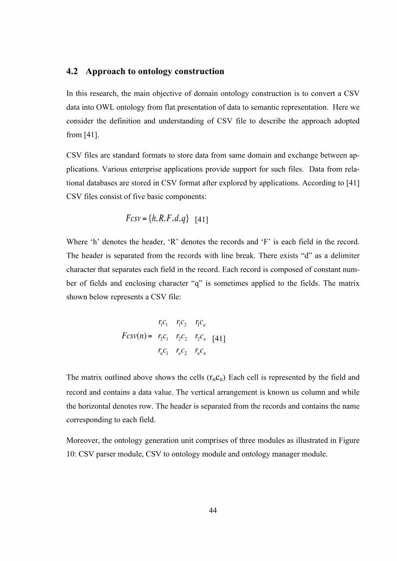
CSV files consist of five basic components:

Fcsv = {h,R,F,d,q} [41]

Where ‘h’ denotes the header, ‘R’ denotes the records and ‘F’ is each field in the record.

The header is separated from the records with line break. There exists “d” as a delimiter

character that separates each field in the record. Each record is composed of constant num-

ber of fields and enclosing character “q” is sometimes applied to the fields. The matrix

shown below represents a CSV file:

Fcsv(n) =r1c1 r1c2 r1cnr2c1 r2c2 r2cnrnc1 rnc2 rncn

[41]

The matrix outlined above shows the cells (rncn). Each cell is represented by the field and

record and contains a data value. The vertical arrangement is known us column and while

the horizontal denotes row. The header is separated from the records and contains the name

corresponding to each field.

Moreover, the ontology generation unit comprises of three modules as illustrated in Figure

10: CSV parser module, CSV to ontology module and ontology manager module.

45

Figure 10: CSV dataset to ontology

The ontology manager module is based on OWL API (see Section 3.7) and handles all op-

eration related to an OWL ontology. The CSV parser module is responsible for parsing of

CSV file into ‘CSVHeader’, ‘CSVclass’ and ‘dataset’. The CSV to ontology module is

responsible for the mapping of CSV file to OWL ontology. The mapping approach consid-

ers the mapping of CSV components outlined above to ontology components. An individu-

al CSV file is considered as a class in OWL ontology. Each record in the CSV file is

mapped to a specific ontology instance and literal values. The headers are mapped to on-

tology properties. In this research we assume all the data stored in a given CSV file refer to

only the current file. However, CSV files can have member records that refer to another

file and such records are mapped as object property [41].

As mentioned in section 3.5.2, properties in ontology have data range with specific data

type. Thus, we adopted the algorithm from [41] to recognize property data types. The

main purpose of recognizing data range of a property is to complete the creation of domain

ontology and automatic formation of data type for a given property. The algorithm adopted

works by considering each non-zero value for a given header. Each value is analyzed

against predicting regular expression and the size of the values checked against the maxi-

mum size allowed for individual data type. If the size is less than the threshold, the process

is repeated for each data type. For instance, if we check a value against a Boolean data type

the maximum threshold is 5, which is the size of “False”. Given Boolean values “yes”,

“no”, “1”, “0”, “T”, ”F”, “True” and “False”.

46

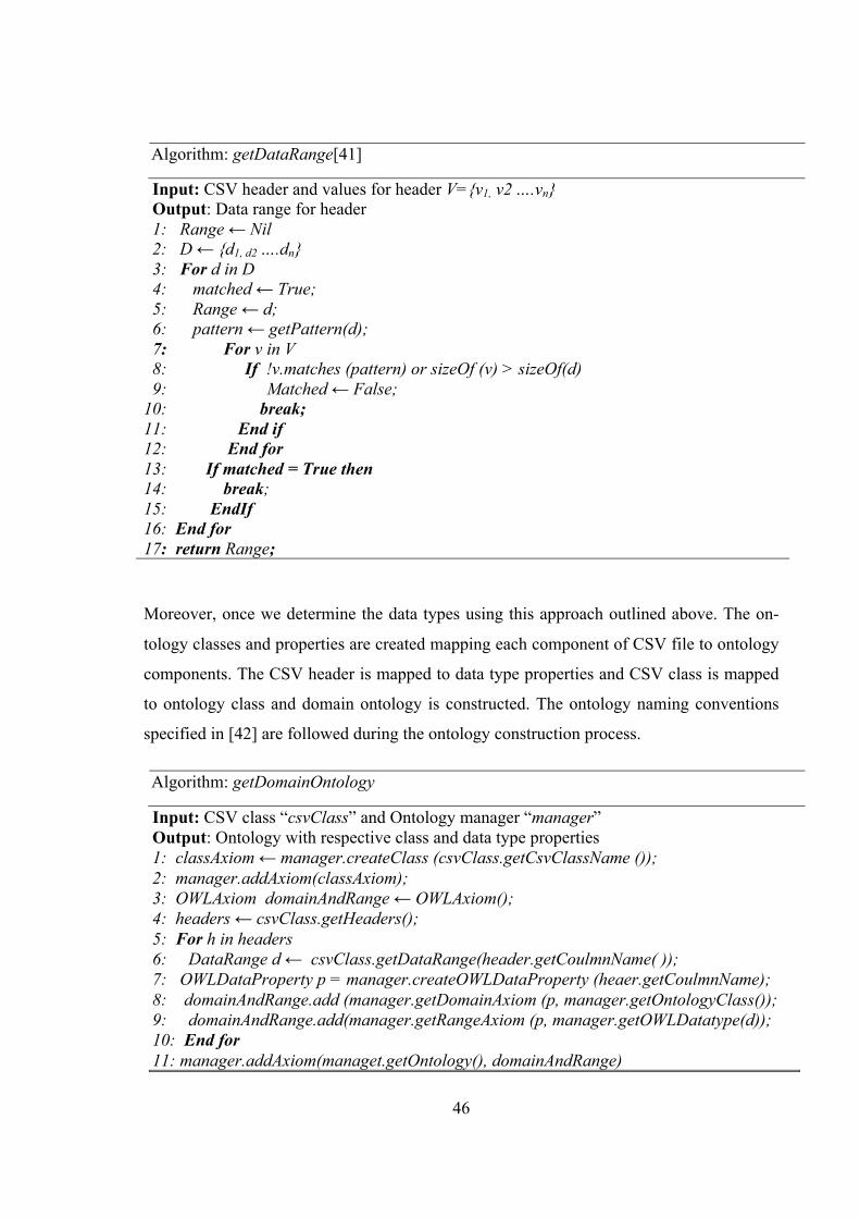
Algorithm: getDataRange[41]

Input: CSV header and values for header V={v1, v2 ….vn} Output: Data range for header 1: Range ← Nil 2: D ← {d1, d2 ….dn} 3: For d in D 4: matched ← True; 5: Range ← d; 6: pattern ← getPattern(d); 7: For v in V 8: If !v.matches (pattern) or sizeOf (v) > sizeOf(d) 9: Matched ← False; 10: break; 11: End if 12: End for 13: If matched = True then 14: break; 15: EndIf 16: End for 17: return Range;

Moreover, once we determine the data types using this approach outlined above. The on-

tology classes and properties are created mapping each component of CSV file to ontology

components. The CSV header is mapped to data type properties and CSV class is mapped

to ontology class and domain ontology is constructed. The ontology naming conventions

specified in [42] are followed during the ontology construction process.

Algorithm: getDomainOntology

Input: CSV class “csvClass” and Ontology manager “manager” Output: Ontology with respective class and data type properties 1: classAxiom ← manager.createClass (csvClass.getCsvClassName ()); 2: manager.addAxiom(classAxiom); 3: OWLAxiom domainAndRange ← OWLAxiom(); 4: headers ← csvClass.getHeaders(); 5: For h in headers 6: DataRange d ← csvClass.getDataRange(header.getCoulmnName( )); 7: OWLDataProperty p = manager.createOWLDataProperty (heaer.getCoulmnName); 8: domainAndRange.add (manager.getDomainAxiom (p, manager.getOntologyClass()); 9: domainAndRange.add(manager.getRangeAxiom (p, manager.getOWLDatatype(d)); 10: End for 11: manager.addAxiom(managet.getOntology(), domainAndRange)

47

Here, we present the examples of ontology construction process with dataset from UCI

repository. We use Wisconsin breast cancer database (WBCD) from UCI repository. Dr.

William H.Wolberg at Wisconsin Hospital collected this dataset. The problem concerns

with the prediction of whether a tissue sample collected from a patient breast is benign or

malignant. The dataset is composed of 699 records, and consists of 2 classes, 10 feature

and 16 records with missing value [46]. Figure-12 shows the snapshot of sample data rec-

ords in Microsoft excel tool.

The dataset is downloaded from university of California database (UCI) into two files;

‘breast-cancer-wisconsin.data’ and ‘breast- cancer-wisconsin.names’. The first file con-

tains information about the dataset including feature names. The second file contains all

the records of the dataset. In order to proceed with the experiment, the two files are com-

bined into same file and saved in CSV format.

The ontology generation unit of the application accepts CSV files where the column data

and all records have no quote. Hence, to avoid unpredictable errors all the quotes are re-

moved in the prepared dataset. The following preprocessing is done in the prepared CSV

data.

• Removal of unsupported quoted characters.

• Correction of delimited text at the end of each line.

• Confirming the CSV file has same delimited text.

• Correction of repeated header names in the file.

Figure 11: Sample WBCD dataset

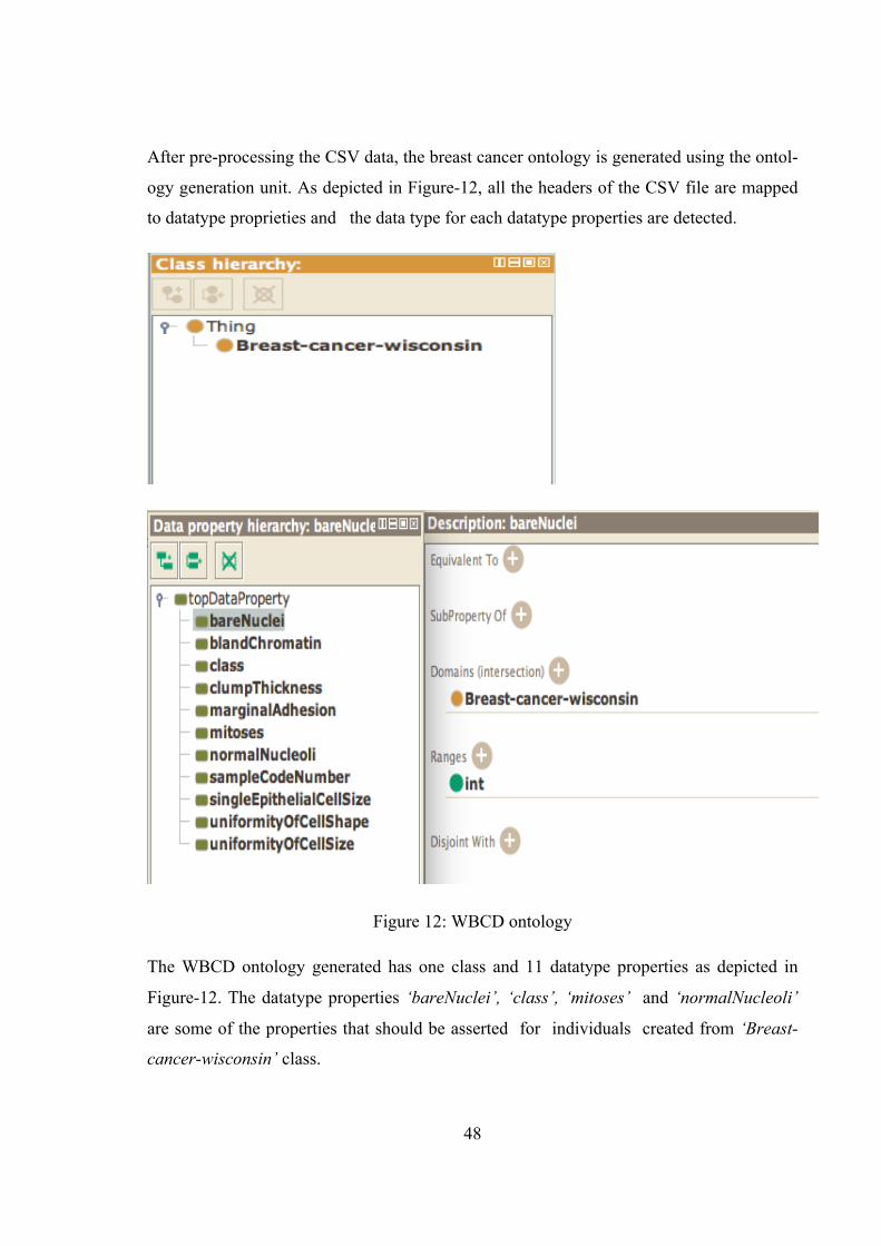
48

After pre-processing the CSV data, the breast cancer ontology is generated using the ontol-

ogy generation unit. As depicted in Figure-12, all the headers of the CSV file are mapped

to datatype proprieties and the data type for each datatype properties are detected.

Figure 12: WBCD ontology

The WBCD ontology generated has one class and 11 datatype properties as depicted in

Figure-12. The datatype properties ‘bareNuclei’, ‘class’, ‘mitoses’ and ‘normalNucleoli’

are some of the properties that should be asserted for individuals created from ‘Breast-

cancer-wisconsin’ class.

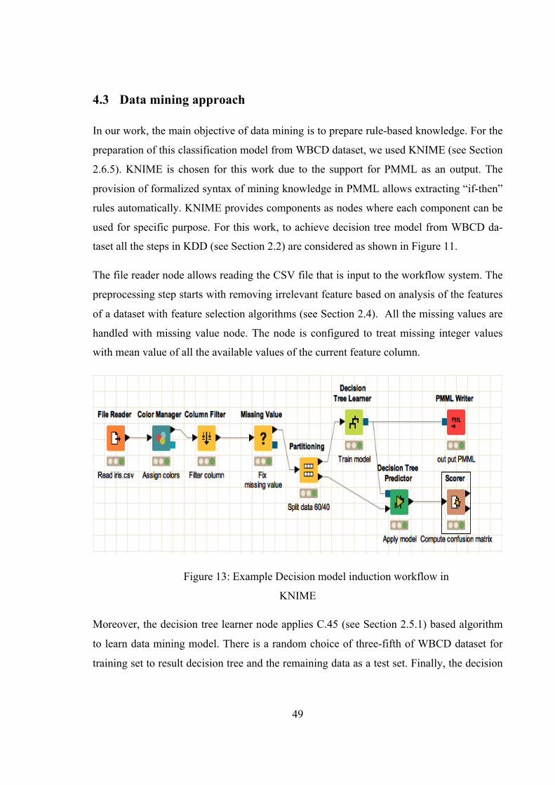
49

4.3 Data mining approach

In our work, the main objective of data mining is to prepare rule-based knowledge. For the

preparation of this classification model from WBCD dataset, we used KNIME (see Section

2.6.5). KNIME is chosen for this work due to the support for PMML as an output. The

provision of formalized syntax of mining knowledge in PMML allows extracting “if-then”

rules automatically. KNIME provides components as nodes where each component can be

used for specific purpose. For this work, to achieve decision tree model from WBCD da-

taset all the steps in KDD (see Section 2.2) are considered as shown in Figure 11.

The file reader node allows reading the CSV file that is input to the workflow system. The

preprocessing step starts with removing irrelevant feature based on analysis of the features

of a dataset with feature selection algorithms (see Section 2.4). All the missing values are

handled with missing value node. The node is configured to treat missing integer values

with mean value of all the available values of the current feature column.

Figure 13: Example Decision model induction workflow in

KNIME

Moreover, the decision tree learner node applies C.45 (see Section 2.5.1) based algorithm

to learn data mining model. There is a random choice of three-fifth of WBCD dataset for

training set to result decision tree and the remaining data as a test set. Finally, the decision

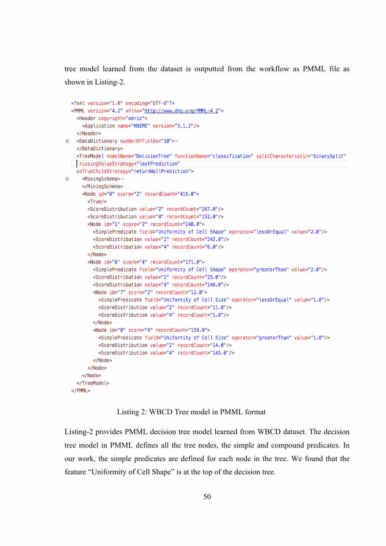
50

tree model learned from the dataset is outputted from the workflow as PMML file as

shown in Listing-2.

Listing 2: WBCD Tree model in PMML format

Listing-2 provides PMML decision tree model learned from WBCD dataset. The decision

tree model in PMML defines all the tree nodes, the simple and compound predicates. In

our work, the simple predicates are defined for each node in the tree. We found that the

feature “Uniformity of Cell Shape” is at the top of the decision tree.

51

4.4 Automatic extraction of inductive rules from PMML

In this section, we present an approach to the extraction of rules from PMML. Here, we

have used XSL style sheet to transform a PMML model into Rule XML. The transfor-

mation style sheets are written for individual DM models (decision tree, association rule)

that are embedded in the PMML file. For instance, the PMML model outlined above in

Listing-2 models decision tree from WBCD dataset and follows a predefined syntax agreed

upon the data-mining group (DMG). Thus we used XSL style sheet customized to PMML

decision tree model as shown in Listing-3 to extract inductive rules. All the data mining

tools that adopt PMML as output generate PMML with syntax provided by DMG, thus a

predefined XSL style sheet works for transforming same type PMML models.

Listing 3: XSL stylesheet for decision tree PMML (version 4.2)

Moreover, the rule generation component contains a mapping module as shown in Figure-

14. The mapping module is responsible for parsing of PMML, selecting appropriate XSL

and handling the transformation of PMML to Rule XML.

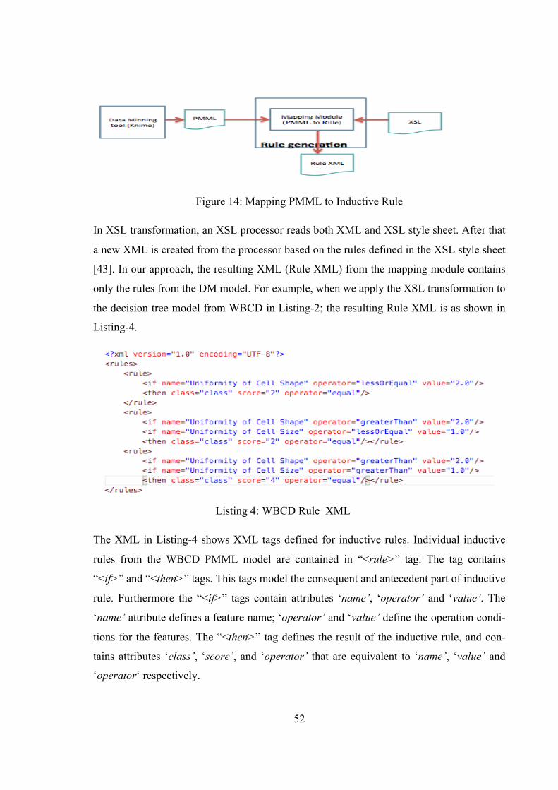
52

Figure 14: Mapping PMML to Inductive Rule

In XSL transformation, an XSL processor reads both XML and XSL style sheet. After that

a new XML is created from the processor based on the rules defined in the XSL style sheet

[43]. In our approach, the resulting XML (Rule XML) from the mapping module contains

only the rules from the DM model. For example, when we apply the XSL transformation to

the decision tree model from WBCD in Listing-2; the resulting Rule XML is as shown in

Listing-4.

Listing 4: WBCD Rule XML

The XML in Listing-4 shows XML tags defined for inductive rules. Individual inductive

rules from the WBCD PMML model are contained in “<rule>” tag. The tag contains

“<if>” and “<then>” tags. This tags model the consequent and antecedent part of inductive

rule. Furthermore the “<if>” tags contain attributes ‘name’, ‘operator’ and ‘value’. The

‘name’ attribute defines a feature name; ‘operator’ and ‘value’ define the operation condi-

tions for the features. The “<then>” tag defines the result of the inductive rule, and con-

tains attributes ‘class’, ‘score’, and ‘operator’ that are equivalent to ‘name’, ‘value’ and

‘operator‘ respectively.

53

4.5 Mapping approach to translate DM model to SWRL

In the previous sections, we described the process of ontology construction from CSV data,

data mining process and inductive rule extraction from PMML. This section will provide

the approach to translate Rule-based knowledge to Semantic Web standard. For this work,

to achieve the Rule-based knowledge in Semantic Web standard, we need to define both

the syntax and semantics of the DM knowledge. Currently, there is no standard defined to

describe the semantics of Rule-based knowledge [4], thus we used SWRL (see Section

3.6).

Moreover, in our approach the PMML rule-based knowledge is translated with the SWRL

generation unit shown in Figure-15. The unit contains mapping module, which is responsi-

ble for the translation of PMML to SWRL.

Figure 15: Mapping PMML to SWRL

The mapping module works with the rule generation module to get Rule XML, which con-

tains the inductive rules extracted from PMML then maps the Rule XML to SWRL. Here

we consider the definition of SWRL and its atoms (see Section 3.6) to describe the ap-

proach of mapping each inductive rule in Rule XML to SWRL atoms.

The Rule XML “<if>” tag represents the body part of the SWRL rule while the “<then>”

tag represents the head part of the SWRL rule (See Listing-4). In order to bridge the semat-

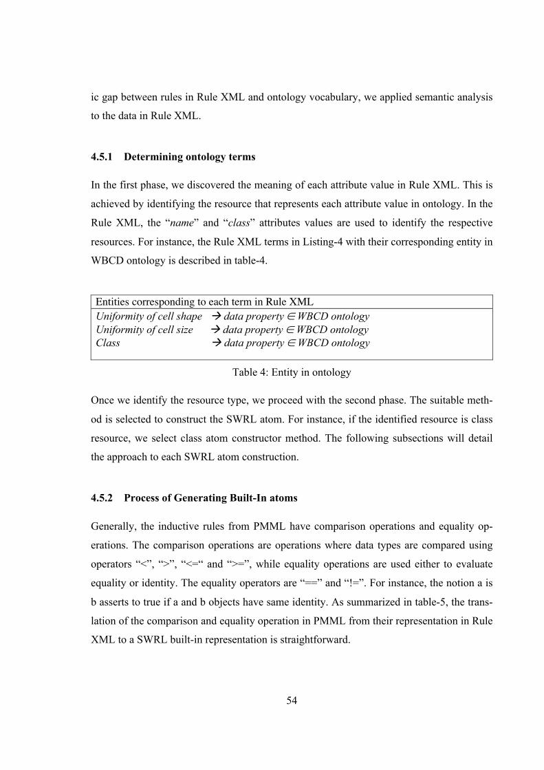
54

ic gap between rules in Rule XML and ontology vocabulary, we applied semantic analysis

to the data in Rule XML.

4.5.1 Determining ontology terms

In the first phase, we discovered the meaning of each attribute value in Rule XML. This is

achieved by identifying the resource that represents each attribute value in ontology. In the

Rule XML, the “name” and “class” attributes values are used to identify the respective

resources. For instance, the Rule XML terms in Listing-4 with their corresponding entity in

WBCD ontology is described in table-4.

Entities corresponding to each term in Rule XML Uniformity of cell shape à data property ∈ WBCD ontology Uniformity of cell size à data property ∈ WBCD ontology Class à data property ∈ WBCD ontology

Table 4: Entity in ontology

Once we identify the resource type, we proceed with the second phase. The suitable meth-

od is selected to construct the SWRL atom. For instance, if the identified resource is class

resource, we select class atom constructor method. The following subsections will detail

the approach to each SWRL atom construction.

4.5.2 Process of Generating Built-In atoms

Generally, the inductive rules from PMML have comparison operations and equality op-

erations. The comparison operations are operations where data types are compared using

operators “<”, “>”, “<=“ and “>=”, while equality operations are used either to evaluate

equality or identity. The equality operators are “==” and “!=”. For instance, the notion a is

b asserts to true if a and b objects have same identity. As summarized in table-5, the trans-

lation of the comparison and equality operation in PMML from their representation in Rule

XML to a SWRL built-in representation is straightforward.

55

Rule XML data SWRL Built-in

Equality operators

notEqual swrlb :notEqual

equal swrlb : equal

Comparison operators

greaterThan swrlb : greaterThan

greaterOrEqual swrlb : greaterOrEqual

lessOrEqual swrlb : lessOrEqual

lessThan swrlb : lessThan

Identity operators

notEqual swrlb : sameAs

equal swrlb : different

Table 5: SWRL Built-in translation reference

Moreover, we need the ontology entity identified with the approach outlined in the previ-

ous section to achieve built-in atom generation. Based on the entity in ontology, we map

the Rule XML data to equivalent SWRL Built-In. For instance, we take inductive rule in

(1) from the Rule XML in Listing4:

(1) >/="2.0" valuel"lessOrEqua="operator Shape" Cell of uniformity="name if<

As summarized in table -4, the entity identified in ontology for “uniformity of cell shape”

is data property. Thus, we consider that the property entity related values are literals (see

Section 3.4). Thus, we use comparison operators for evaluating data types. Therefore, the

Rule XML operator value ‘lessOrEqual’ is mapped to equivalent SWRL Built-In

‘swrlb:lessOrEqual’. The rule in (2) represents a condition of the data property restricted

with its domain.

Breast-cancer-wisconsin(?y,?x)∧uniformityOfCellShape(?x) ∧ swrlb:lessOrEqual(?x,2.0) (2)

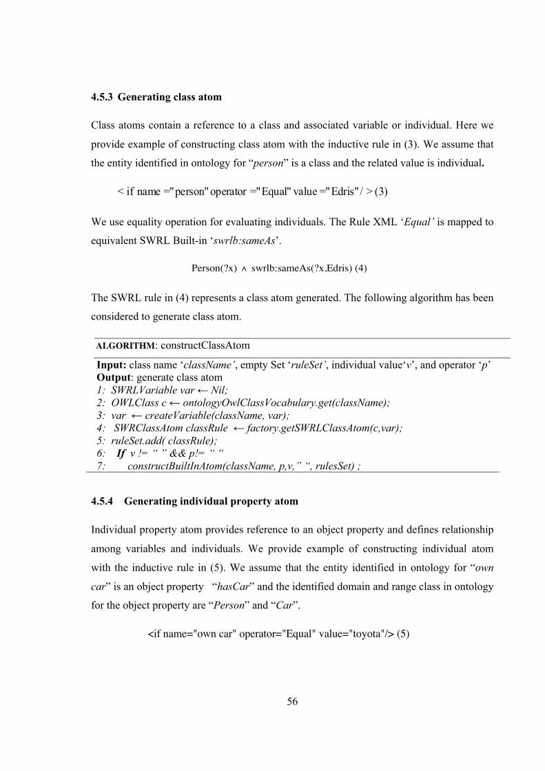
56

4.5.3 Generating class atom

Class atoms contain a reference to a class and associated variable or individual. Here we

provide example of constructing class atom with the inductive rule in (3). We assume that

the entity identified in ontology for “person” is a class and the related value is individual.

(3) >/Edris"=" valueEqual"="operator person"="name if<

We use equality operation for evaluating individuals. The Rule XML ‘Equal’ is mapped to

equivalent SWRL Built-in ‘swrlb:sameAs’.

Person(?x) ∧ swrlb:sameAs(?x,Edris) (4)

The SWRL rule in (4) represents a class atom generated. The following algorithm has been

considered to generate class atom.

ALGORITHM: constructClassAtom

Input: class name ‘className’, empty Set ‘ruleSet’, individual value‘v’, and operator ‘p’ Output: generate class atom 1: SWRLVariable var ← Nil; 2: OWLClass c ← ontologyOwlClassVocabulary.get(className); 3: var ← createVariable(className, var); 4: SWRClassAtom classRule ← factory.getSWRLClassAtom(c,var); 5: ruleSet.add( classRule); 6: If v != “ ” && p!= “ “ 7: constructBuiltInAtom(className, p,v,” “, rulesSet) ;

4.5.4 Generating individual property atom

Individual property atom provides reference to an object property and defines relationship

among variables and individuals. We provide example of constructing individual atom

with the inductive rule in (5). We assume that the entity identified in ontology for “own

car” is an object property “hasCar” and the identified domain and range class in ontology

for the object property are “Person” and “Car”.

<if name="own car" operator="Equal" value="toyota"/> (5)

57

We use equality operation for evaluating individuals. The Rule XML ‘Equal’ is mapped to

equivalent SWRL Built-in ‘swrlb:sameAs’. Furthermore, a class atom is created for the

domain and range classes identified.

Person(?x)∧Car(?y) ∧hasCar(? x,? y)∧ swrlb:sameAs(?y,toyota) (6)

The SWRL rule in (6) represents an individual property atom generated with the domain

and range restrictions. The following algorithm has been considered to generate individual

property atoms.

ALGORITHM: constructindividualAtom

Input: class name ‘objectName’, empty Set ‘ruleSet’, individual value‘v’, and operator ‘p’ Output: generate individual atom 1: SWRLVariable var1, var2 ← Nil; 2: OWLObjectProperty o← OWLObjectPropertyVocabulary.get(objectName); 3: classSubjectName ← constructtSubjectClassAtom(objectName, ruleSet); 4: classObjectName ← constructObjectClassAtom(objectName, ruleSet); 5: var1 ← createVariable(classSubjectName, var1); 6: var2 ← createVariable(classObjectName, var2); 7: ruleSet.add(factory.getSWRLObjectAtom(o,var1,var2);); 8: constructBuiltInAtom(classObjectName, p,v,” “, rulesSet) ;

4.5.5 Generating data valued atom

Data valued atom contains a reference to a datatype property, class and associated variable.

For instance, we take inductive rule in (7) from the Rule XML in Listing-4:

<if name="uniformity of Cell Size" operator="lessOrEqual" value="1.0"/> (7)

As summarized in table-4, the entity identified in ontology for “uniformity of cell size” is

data property. Thus, we consider that the property entity related values are literal (see Sec-

tion 3.4). Thus, we use comparison operators for evaluating data types. The Rule XML

‘lessOrEqual’ is mapped to equivalent SWRL Built-in ‘swrlb:lessOrEqual’.

Breast-cancer-wisconsin(?y,?x)∧uniformityOfCellSize(?x) ∧ swrlb:lessOrEqual(?x,1.0) (8)

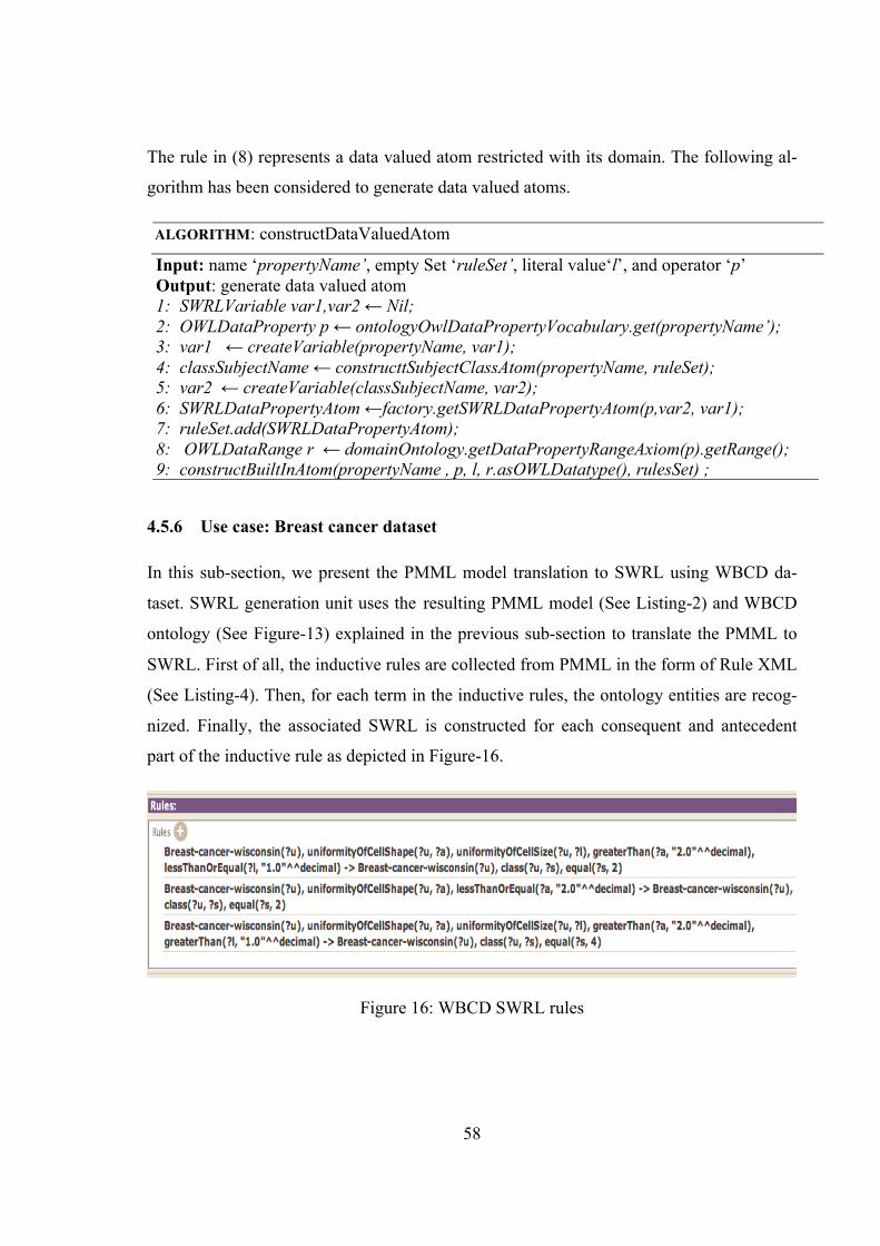
58

The rule in (8) represents a data valued atom restricted with its domain. The following al-

gorithm has been considered to generate data valued atoms.

ALGORITHM: constructDataValuedAtom

Input: name ‘propertyName’, empty Set ‘ruleSet’, literal value‘l’, and operator ‘p’ Output: generate data valued atom 1: SWRLVariable var1,var2 ← Nil; 2: OWLDataProperty p ← ontologyOwlDataPropertyVocabulary.get(propertyName’); 3: var1 ← createVariable(propertyName, var1); 4: classSubjectName ← constructtSubjectClassAtom(propertyName, ruleSet); 5: var2 ← createVariable(classSubjectName, var2); 6: SWRLDataPropertyAtom ←factory.getSWRLDataPropertyAtom(p,var2, var1); 7: ruleSet.add(SWRLDataPropertyAtom); 8: OWLDataRange r ← domainOntology.getDataPropertyRangeAxiom(p).getRange(); 9: constructBuiltInAtom(propertyName , p, l, r.asOWLDatatype(), rulesSet) ;

4.5.6 Use case: Breast cancer dataset

In this sub-section, we present the PMML model translation to SWRL using WBCD da-

taset. SWRL generation unit uses the resulting PMML model (See Listing-2) and WBCD

ontology (See Figure-13) explained in the previous sub-section to translate the PMML to

SWRL. First of all, the inductive rules are collected from PMML in the form of Rule XML

(See Listing-4). Then, for each term in the inductive rules, the ontology entities are recog-

nized. Finally, the associated SWRL is constructed for each consequent and antecedent

part of the inductive rule as depicted in Figure-16.

Figure 16: WBCD SWRL rules

59

5 Limitation and challenges

1. Standardized discoverable rule: Currently, there is no standard to represent the seman-

tics of discoverable knowledge [4]. The researches focused more on the representation

of the syntax of DM knowledge and PMML is one of the results of this research. Thus,

we propose SWRL to be used to describe the semantics of knowledge discovery.

2. Ontology construction Issues: In order to construct machine “understandable” rule-

based knowledge; we need to properly define not only the syntax, but also the seman-

tics of the rules. In our approach the SWRL is used to define the semantics and syntax.

We discussed that SWRL is described using concepts from ontology. Thus, the proper

hierarchical definition of the concepts in ontology is necessary. In our work, we con-

structed temporary ontologies using semi-automatic approach. Hence, we achieved a

knowledge base for the translation process. However, we discovered that the ontology

generated lacks proper hierarchical definition. As a result, an alignment feature needs

to be integrated into the system to map our ontology to domain ontology designed by

an expert in the domain.

3. Lack of querying mechanism: We discussed ontology building tools and frameworks.

The protégé tool allows manually building ontology and also reviewing ontologies

built with the ontology frameworks. We studied OWL API is used for management,

reasoning and validation of ontology programmatically. Currently, querying mecha-

nism is not integrated in OWL API [34]. Thus, when building SWRL atoms that re-

quire querying functionalities becomes tedious.

4. Issues over Data mining tools: We studied the open source DM tools including WEKA

and KNIME. The tools are used to discover a DM model from a dataset. However, the

tools out put the data-mining model in different format. Some support PMML, which is

a standard for storing DM model. In our research, we identified that an output model

from WEKA tool doesn’t provide programmable interface. In addition we found out

that KNIME sometimes generates non-standard PMML as an output.

60

6 Conclusion

This thesis tried to give an answer to the following research questions

1. How can we translate PMML based data mining model to Semantic Web standard?

2. How to design automatic translation of PMML data mining model to Semantic

Web standard?

To answer the first research question we covered preliminary studies on Semantic Web,

predictive knowledge algorithms, frameworks for ontology management and data mining

tools. We also proposed approach learning from the research to achieve translation of

PMML model to Semantic Web standard.

The secondary goal of the research was to propose a design that allows achieving automat-

ic translation of PMML to SWRL. In chapter-4, we proposed design architecture for

PMML to SWRL translation. We discussed a model to learn temporary ontology from a

dataset so as to provide a knowledge based for the translation. We used semi-automatic

approach to learn the ontology in our work. However, we discovered that the ontology

generated lacks proper hierarchical definition. Hence, for a better performance of the trans-

lation results, an alignment feature needs to be integrated into the system to align our tem-

porary ontology to domain ontology designed by an expert in the domain.

Moreover, we described an approach to discover data mining knowledge in PMML format.

Furthermore, we provided a description on how to extract individual rules in PMML model

to support the translation to SWRL. Studying the various tools and methods gave the re-

quired information to continue with the setup and implementation of the project performed.

We picked a sample data from UCI repository dataset and carried out tests to explain each

implementation’s point of view. The results from the use case showed that, it is possible to

achieve an automatic translation of PMML model to semantic web standard (SWRL).

61

7 Reference:

1. Goebel, Michael, and Le Gruenwald. "A survey of data mining and knowledge dis-

covery software tools." ACM SIGKDD Explorations Newsletter 1.1 (1999): 20-33.

2. Guazzelli, Alex, et al. "PMML: An open standard for sharing models." The R Jour-

nal 1.1 (2009): 60-65.

3. Berners-Lee, T., Hendler, J., Lassila, O.: The Semantic Web. Scientific American

284(5) (May 2001)

4. Dejing Dou, Han Qin, and Haishan Liu: Semantic Translation for Rule-Based

Knowledge in Data Mining

5. Pukkhem, Noppamas :A Semantic-based Approach for Representing Successful

Graduate Predictive Rules

6. S. B. Kotsiantis, Supervised Machine Learning: A Review of Classification Tech-

niques, Proceedings of the 2007 conference on Emerging Artificial Intelligence Ap-

plications in Computer Engineering: Real Word AI Systems with Applications in

eHealth, HCI, Information Retrieval and Pervasive Technologies, p.3-24, June 10,

2007.

7. Apté, Chidanand, and Sholom Weiss. "Data mining with decision trees and decision

rules." Future generation computer systems 13.2 (1997): 197-210.

8. Wu, Xindong, et al. "Top 10 algorithms in data mining." Knowledge and Information

Systems 14.1 (2008): 1-37.

9. Weiss, Sholom M. et al., Predictive Data-Mining: A Practical Guide. San Francisco,

Morgan Kaufmann (1998).

10. Usama, M. Fayyad, "Data-Mining and Knowledge Discovery: Making Sense Out of

Data," Microsoft Research IEEE Expert, 11:5. (1996), pp. 20-25.

11. A Comparative Analysis Of Predictive Data-Mining Techniques Godswill

Chukwugozie Nsofor August, 2006

12. Practical machine learning tools and techniques Ian H. Witten , Eibe Frank , 2005

13. Murthy, (1998), Automatic Construction of Decision Trees from Data: A Multi-

Disciplinary Survey, Data Mining and Knowledge Discovery 2: 345–389.

62

14. Quinlan, J.R. (1993). C4.5: Programs for machine learning. Morgan Kaufmann, San

Francisco.

15. Wuermli, O., Wrobel, A., Hui S. C. and Joller, J. M. “Data Mining For Ontolo-

gy_Building: Semantic Web Overview”, Diploma Thesis–Dep. of Computer Sci-

ence_WS2002/2003, Nanyang Technological University.

16. Yoav Freund and Llew Mason. The alternating decision tree-learning algorithm.

In Proc. 16th International Conf. on Machine Learning, pages 124--133, 1999.

17. Quinlan, J. Ross. "Generating Production Rules from Decision Trees." IJCAI. Vol.

87. 1987.

18. R Agrawal, R Srikant" Fast algorithms for mining association rules"

Proc. 20th int. conf. very large databases, VLDB 1215, 487-499

19. Guyon, Isabelle, and André Elisseeff. "An introduction to variable and feature selec-

tion." Journal of machine learning research 3.Mar (2003): 1157-1182

20. Molina, Luis Carlos, Lluís Belanche, and Àngela Nebot. "Feature selection algo-

rithms: a survey and experimental evaluation." Data Mining, 2002. ICDM 2003. Pro-

ceedings. 2002 IEEE International Conference on. IEEE, 2002

21. Jovic, Alan, Karla Brkic, and Nikola Bogunovic. "An overview of free software tools

for general data mining." Information and Communication Technology, Electronics

and Microelectronics (MIPRO), 2014 37th International Convention on. IEEE, 2014.

22. Subathra, P., et al. "A Study of Open Source Data Mining Tools and its Applica-

tions." Research Journal of Applied Sciences, Engineering and Technology 10.10

(2015): 1108-1132.

23. Berners-Lee, Tim. "RFC 1630,"." Universal Resource Identifiers in WWW: A Unify-

ing Syntax for the Expression of Names and Addresses of Objects on the Network as

used in the World-Wide Web (1994).

24. Berners-Lee, Tim, Larry Masinter, and Mark McCahill. Uniform resource locators

(URL). No. RFC 1738. 1994.

25. Identifiers, Internationalized Resource. The Internet Engineering Task Force

(IETF).[Online] http://www. w3. org/TR/2009/REC-owl2-primer-20091027/# ref-rfc-

3987. RFC 3987.

26. Powers, Shelley. Practical rdf. " O'Reilly Media, Inc.", 2003.

63

27. 2. J. J. Carroll and G. Klyne, “Resource description framework (RDF): Concepts and

abstract syntax,” W3C recommendation, W3C, Feb. 2004. http://www.

w3.org/TR/2004/REC-rdf-concepts-20040210/.

28. R. V. Guha and D. Brickley, “RDF vocabulary description language 1.0: RDF sche-

ma,” W3C candidate recommendation, W3C, Mar. 2000. http://www.

w3.org/TR/2000/CR-rdf-schema-20000327/.

29. P. Hayes, P. F. Patel-Schneider, and I. Horrocks, “OWL web ontology language se-

mantics and abstract syntax,” W3C recommendation, W3C, Feb. 2004. http:

//www.w3.org/TR/2004/REC-owl-semantics-20040210/.

30. W3C OWL Working Group, “OWL 2 web ontology language document overview,”

tech. rep., W3C, Oct. 2009. http://www.w3.org/TR/2009/ REC-owl2-overview-

20091027/.

31. SWRLSubmission,http://www.w3.org/Submission/SWRL/

32. CaliforniaDriverHandbook,http://www.dmv.ca.gov/pubs/dl600.pdf

33. Horridge, M. (2009). A Practical Guide To Building OWL Ontologies Using Protégé

4 and CO-ODE Tools. The University Of Manchester. Retrieved from

http://owl.cs.manchester.ac.uk/tutorials/protegeowltutorial/resources/Protege OWL-

TutorialP4_v1_2.pdf

34. Horridge, M and Bechofer S, "The OWL API :A Java API for OWL Ontologies"

35. Motik, Boris and Patel-Schneider, Peter F. and Parsia, Bi- jan. OWL 2 Web Ontology

Language Structural Specification and Functional-Style Syntax. W3C Recommenda-

tion, World Wide Web Consortium, 2009. http://www.w3.org/TR/ owl2- syntax/.

36. Erich Gamma, Richard Helm, Ralph Johnson, and John Vlis- sides. Design Patterns:

Elements of Reusable Object-Oriented Software. Professional Computing Series. Ad-

dison-Wesley, 1995.

37. A SURVEY ON ONTOLOGY CONSTRUCTION METHODOLOGIES,

R.Subhashini and Dr. J. Akilandeswari -2011

38. Maizatul Akmar Ismail, Mashkuri Y aacob & Sameem Abdul Kareem, 2006. Ontolo-

gy Construction: An Overview, Malaysia.

64

39. [Millerym. 2007] MillerG.A.,FellbaumC.,TengiR.ym.,WordNet lexical database for

the English language, Cognitive Science Laboratory, Princeton University,

<http://wordnet.princeton.edu/>, viitattu 12.2.2007.

40. Bache, K., Lichman, M.: UCI machine learning repository (2013)

41. Automatically converting tabular data to rdf: an ontological approach Kumar Sharma,

Ujjal Marjit, and Utpal Biswas

42. Style Guidelines for Naming and Labeling Ontologies in the Multilingual Web Elena

Montiel-Ponsoda, Daniel Vila-Suero, and Boris Villazón-Terraza

43. Harold, Elliotte Rusty. XML 1.1 Bible. Vol. 136. John Wiley & Sons, 2004.

44. Java Libraries for Accessing the Princeton Wordnet: Comparison and Evaluation.

Mark Alan Finlayson

45. Hebeler, John, et al. Semantic Web programming. John Wiley & Sons, 2011

46. K. P. Bennett & O. L. Mangasarian: "Robust linear programming discrimination of

two linearly inseparable sets", Optimization Methods and Software 1, 1992, 23-34

(Gordon & Breach Science Publishers).

47. F.Grivokostopoulou , I.Perikos , I.Hatzilygeroudis : “Utilizing Semantic Web

Technologies and Data Mining Techniques to Analyze Students Learning and Predict

Final Performance”