Embed Size (px)
Citation preview

i

ii
Editorial Board Dr. Zafer Omer Ozdemir
Energy Systems Engineering Kırklareli, Kirklareli University, Turkey
Dr. H.Saremi
Vice- chancellor For Adminstrative& Finance Affairs, Islamic Azad university of Iran, Quchan branch,
Quchan-Iran
Dr. Ahmed Kadhim Hussein
Department of Mechanical Engineering, College of Engineering, University of Babylon, Republic of Iraq
Mohammad Reza Kabaranzad Ghadim
Associated Prof., Department of Management, Industrial Management, Central Tehran Branch, Islamic
Azad University, Tehran, Iran
Prof. Ramel D. Tomaquin
Prof. 6 in the College of Business and Management, Surigao del Sur State University (SDSSU), Tandag
City ,Surigao Del Sur, Philippines
Dr. Ram Karan Singh
BE.(Civil Engineering), M.Tech.(Hydraulics Engineering), PhD(Hydraulics & Water Resources
Engineering),BITS- Pilani, Professor, Department of Civil Engineering,King Khalid University, Saudi
Arabia.
Dr. Asheesh Kumar Shah
IIM Calcutta, Wharton School of Business, DAVV INDORE, SGSITS, Indore
Country Head at CrafSOL Technology Pvt.Ltd, Country Coordinator at French Embassy, Project
Coordinator at IIT Delhi, INDIA
Dr. Uma Choudhary
Specialization in Software Engineering Associate Professor, Department of Computer Science Mody
University, Lakshmangarh, India
Dr. Ebrahim Nohani
Ph.D.(hydraulic Structures), Department of hydraulic Structures,Islamic Azad University, Dezful, IRAN.
Dr.Dinh Tran Ngoc Huy
Specialization Banking and Finance, Professor,Department Banking and Finance , Viet Nam
Dr. Shuai Li Computer Science and Engineering, University of Cambridge, England, Great Britain
Dr. Ahmadad Nabih ZakiRashed
Specialization Optical Communication System,Professor,Department of Electronic Engineering,
Menoufia University
iii
Dr.Alok Kumar Bharadwaj
BE(AMU), ME(IIT, Roorkee), Ph.D (AMU),Professor, Department of Electrical Engineering, INDIA
Dr. M. Kannan
Specialization in Software Engineering and Data mining, Ph.D, Professor, Computer Science,SCSVMV
University, Kanchipuram, India
Dr.Sambit Kumar Mishra
Specialization Database Management Systems, BE, ME, Ph.D,Professor, Computer Science Engineering
Gandhi Institute for Education and Technology, Baniatangi, Khordha, India
Dr. M. Venkata Ramana
Specialization in Nano Crystal Technology, Ph.D,Professor, Physics,Andhara Pradesh, INDIA
Dr.Swapnesh Taterh
Ph.d with Specialization in Information System Security, Associate Professor, Department of Computer
Science Engineering
Amity University, INDIA
Dr. Rabindra Kayastha
Associate Professor, Department of Natural Sciences, School of Science, Kathmandu University, Nepal
Amir Azizi
Assistant Professor, Department of Industrial Engineering, Science and Research Branch-Islamic Azad
University, Tehran, Iran
Dr. A. Heidari
Faculty of Chemistry, California South University (CSU), Irvine, California, USA
DR. C. M. Velu
Prof.& HOD, CSE, Datta Kala Group of Institutions, Pune, India
Dr. Sameh El-Sayed Mohamed Yehia
Assistant Professor, Civil Engineering(Structural), Higher Institute of Engineering -El-Shorouk Academy,
Cairo, Egypt
Dr. Hou, Cheng-I
Specialization in Software Engineering, Artificial Intelligence, Wisdom Tourism, Leisure Agriculture and
Farm Planning, Associate Professor, Department of Tourism and MICE, Chung Hua University, Hsinchu
Taiwan
Branga Adrian Nicolae
Associate Professor, Teaching and research work in Numerical Analysis, Approximation Theory and
Spline Functions, Lucian Blaga University of Sibiu, Romania

iv
Dr. Amit Rathi
Department of ECE, SEEC, Manipal University Jaipur, Rajasthan, India
Dr. Elsanosy M. Elamin
Dept. of Electrical Engineering, Faculty of Engineering. University of Kordofan, P.O. Box: 160, Elobeid,
Sudan

v
FOREWORD
I am pleased to put into the hands of readers Volume-4; Issue-1: Jan, 2018 of “International Journal of Advanced
Engineering, Management and Science (IJAEMS) (ISSN: 2354-1311)” , an international journal which publishes peer
reviewed quality research papers on a wide variety of topics related to Science, Technology, Management and Humanities.
Looking to the keen interest shown by the authors and readers, the editorial board has decided to release print issue also, but this
decision the journal issue will be available in various library also in print and online version. This will motivate authors for quick
publication of their research papers. Even with these changes our objective remains the same, that is, to encourage young
researchers and academicians to think innovatively and share their research findings with others for the betterment of mankind.
This journal has DOI (Digital Object Identifier) also, this will improve citation of research papers.
I thank all the authors of the research papers for contributing their scholarly articles. Despite many challenges, the entire editorial
board has worked tirelessly and helped me to bring out this issue of the journal well in time. They all deserve my heartfelt
thanks.
Finally, I hope the readers will make good use of this valuable research material and continue to contribute their research finding
for publication in this journal. Constructive comments and suggestions from our readers are welcome for further improvement of
the quality and usefulness of the journal.
With warm regards.
Dr. Uma Choudhary
Editor-in-Chief
Date: Jan, 2018

vi
Vol-4, Issue-1, January, 2018
Sr No. Title
1 Numerical simulation of biodiversity: comparison of changing initial conditions and fixed
length of growing season
Author: Atsu J. U., Ekaka-a E.N.
DOI: 10.22161/ijaems.4.1.1
Page No: 001-003
2 Numerical and Statistical Quantifications of Biodiversity: Two-At-A-Time Equal Variations
Author: Ekaka-a E.N., Osahogulu D.J., Atsu J. U., Isibor L. A.
DOI: 10.22161/ijaems.4.1.2
Page No: 004-009
3 Modelling the effects of decreasing the inter–competition coefficients on biodiversity loss
Author: Ekaka-a E. N., Eke Nwagrabe, Atsu J. U.
DOI: 10.22161/ijaems.4.1.3
Page No: 010-013
4 Simulation modelling of the effect of a random disturbance on biodiversity of a
mathematical model of mutualism between two interacting yeast species
Author: Eke Nwagrabe, Atsu J. U., Ekaka-a E. N
DOI: 10.22161/ijaems.4.1.4
Page No: 014-018
5 Study of a Laboratory-based Gamma Spectrometry for Food and Environmental Samples
Author: M. N. Islam, H. Akhter, M. Begum, Y. Mawla, M. Kamal
DOI: 10.22161/ijaems.4.1.5
Page No: 019-023
6 Deterministic Stabilization of a Dynamical System using a Computational Approach
Author: Isobeye George, Jeremiah U. Atsu, Enu-Obari N. Ekaka-a
DOI: 10.22161/ijaems.4.1.6
Page No: 024-028
7 Simulation modeling of the sensitivity analysis of differential effects of the intrinsic growth
rate of a fish population: its implication for the selection of a local minimum
Author: Nwachukwu Eucharia C., Ekaka-a Enu-Obari N., Atsu Jeremiah U.
DOI: 10.22161/ijaems.4.1.7
Page No: 029-034
8 Rates of Soft Ground Tunneling in Vicinity of Existing Structures
Author: Ayman S. Shehata, Adel M. El-Kelesh, Al-Sayed E. El-kasaby, Mustafa Mansour
DOI: 10.22161/ijaems.4.1.8
Page No: 035-045

vii
9 Packing Improvement by using of Quality Function Deployment Method: A Case Study in
Spare Part Automotive Industry in Indonesia
Author: Humiras Hardi Purba, Adi Fitra , Gidionton Saritua Siagian, Widodo Dumadi
DOI: 10.22161/ijaems.4.1.9
Page No: 046-053
10 Gravitational Model to Predict the Megalopolis Mobility of the Center of Mexico
Author: Juan Bacilio Guerrero Escamilla, Sócrates López Pérez, Yamile Rangel Martínez,
Silvia Mendoza Mendoza
DOI: 10.22161/ijaems.4.1.10
Page No: 054-065
11 Artificial Neural Network Controller for Reducing the Total Harmonic Distortion (THD) in
HVDC
Author: Dr. Ali Nathem Hamoodi, Rasha Abdul-nafaa Mohammed
DOI: 10.22161/ijaems.4.1.11
Page No: 066-073
12 Quantic Analysis of Formation of a Biomaterial of Latex, Retinol, and Chitosan for
Biomedical Applications
Author: Karina García-Aguilar, Iliana Herrera-Cantú, Erick Pedraza-Gress, Lillhian Arely
Flores-Gonzalez, Manuel Aparicio-Razo, Oscar Sánchez-Parada, Emmanuel Vázquez-López,
Juan Jesús García-Mar, Manuel González-Pérez
DOI: 10.22161/ijaems.4.1.12
Page No: 074-079

International Journal of Advanced Engineering, Management and Science (IJAEMS) [Vol-4, Issue-1, Jan- 2018]
https://dx.doi.org/10.22161/ijaems.4.1.1 ISSN: 2454-1311
www.ijaems.com Page | 1
Numerical simulation of biodiversity:
comparison of changing initial conditions and
fixed length of growing season Atsu, J. U.1; Ekaka-a, E.N.2
1Department of Mathematics/Statistics, Cross River University of Technology, Calabar, Nigeria
2Department of Mathematics, Rivers State University, Nkpolu, Port – Harcourt, Nigeria
Abstract— This study examined the effect of varying the
initial value of industrialization for a fixed length of
growing season on the prediction of biodiversity loss. We
have found that when the initial value of industrialization
is 0.1 under a shorter length of growing season, a relative
low due of biodiversity loss can be maintained. The
biodiversity loss value can be further lowered by
maintaining the same length of growing season but with a
reduced initial value of industrialization to 0.01 or 0.02.
We would expect this alternative result to provide a further
insight into our fight against biodiversity loss which has
both human and sustainable development devastating
effects.
Keywords— varying initial data, industrialization,
numerical simulation, growing season, quantitative
technique, forestry resources biomass.
I. INTRODUCTION
The vulnerability of the forest resource biomass to the
ecological risk of biodiversity loss is one of the major
concerns for experts working on the mitigation measures
of forest conservation and sustainable development. In
order to circumvent this ongoing environmental problem,
we have proposed to study the effect of the synergistic
variation of the initial data value of industrialization and a
fixed length of the growing season that has previously
predicted a high volume of biodiversity loss. Atsu and
Ekaka-a (2017) in modeling the intervention with respect
to biodiversity loss, considered changing length of
growing season for a forestry resource biomass. Their
result showed that a longer length of growing season
dominantly predicts a biodiversity gain and vice versa.
Hooper et al (2012) examined a global synthesis which
reveals biodiversity loss over time as a major driver of the
accompanying ecosystem change. In their study, global
environmental changes over time were considered with no
consideration given to initial data of species resources
biomass. In the same context, Isbell et al (2015) showed
that biodiversity increases the resistance of ecosystem
productivity to climate extremes. This was however
without recourse to the underlying factors that sustain
biodiversity and even quantitatively.
Tilman et al (2014) undertook a study which showed that
species diversity is a major determinant of ecosystem
productivity, stability, invasibility and nutrient dynamics.
This paper did not consider a quantitative technique that
can be used to maintain species diversity. Aerts and
Honnay (2011) did research on forest restoration,
biodiversity and ecosystem function. Their result
qualitatively showed that restoring multiple forest
functions requires multiple species.
Naeem et al (1999) did a biological essay that suggests that
biodiversity and ecosystem functioning are necessary
drivers of natural life support processes. It is pertinent to
point out that in all these papers, quantitative examination
of the factors responsible for biodiversity richness and
ecosystem functioning was left out. Reich et al (2012)
showed qualitatively that the impacts of biodiversity loss
escalate through time as redundancy fades but without a
quantitative technique.
This research idea is therefore expected to quantitatively
select the relatively best-fit initial value of industrialization
that will indicate a decrease in biodiversity loss. We will
use a computationally efficient numerical scheme called
Ruge-Kutta ordinary differential equation of order 4-5
(ODE 45) to tackle this challenging environmental
problem when the length of the growing season is five (5)
months with a varying trend.
II. MATHEMATICAL FORMULATIONS
The method that we have proposed to analyse our research
problem has considered the following simplifying
assumptions:
i. The growth of forestry resources biomass and human
population is governed by a logistic type equation.
ii. The growth rate of population pressure is
proportional to the density of human population.
iii. The depletion of the forestry resources is due to
human population and population related activities.

International Journal of Advanced Engineering, Management and Science (IJAEMS) [Vol-4, Issue-1, Jan- 2018]
https://dx.doi.org/10.22161/ijaems.4.1.1 ISSN: 2454-1311
www.ijaems.com Page | 2
Based on these simplifying assumptions the governing
equations of the model according to Ramdhani, Jaharuddin
& Nugrahani (2015) are defined by 𝑑𝐵
𝑑𝑡= 𝑠 (1 −
𝐵
𝐿) 𝐵 − 𝑠. 𝐵 − 𝛽2𝑁𝐵 − 𝑠1𝐼𝐵 − 𝛽3𝐵2𝐼 (1)
𝑑𝑁
𝑑𝑡= 𝑟 (1 −
𝑁
𝐾) 𝑁 − 𝑟0𝑁 + 𝛽1𝑁𝐵 - (2)
𝑑𝑃
𝑑𝑡= 𝜆𝑁 − 𝜆0𝑃 − 𝜃𝐼 - - (3)
𝑑𝐼
𝑑𝑡= 𝜋𝜃𝑃 + 𝜋1𝑠1𝐼𝐵 − 𝜃0𝐼 - - (4)
With the initial condition 𝐵(0) ≥ 0, 𝑁(0) ≥ 0, 𝑃(0) ≥
0, 𝐼(0) ≥ 0 and 0 < 𝜋 ≤ 1,0 < 𝜋1 ≤ 1
In this context, 𝐵 isthe density of forestry resources
biomass with its intrinsic growth rate coefficient s and
carrying capacity L, N represents the density of the human
population, P is the population pressure density while I is
the density of industrialization 𝑠0 represents the coefficient
of the natural depletion rate of resources biomass, ro is the
coefficient of natural depletion rate of human population, r
is the intrinsic growth rate of population density, K
represents the carrying capacity of the population density,
𝛽1 is the growth rate of cumulative density of human
population effect of resources, 𝛽2 is the depletion rate
coefficient of the resource biomass density due to
population. We recognize λ as the growth rate coefficient
of population pressure while 𝜆0 is its natural depletion rate
coefficient, θ is its depletion rate coefficient due to
industrialization, 𝑠1 is the coefficient of depletion rate of
the biomass density as a result of industrialization, the
combined effect of 𝜋1𝑠1 is the growth rate of
industrialization due to forestry resources, 𝜋 is the growth
rate of industrialization effect of population pressure, 𝜃0 is
the coefficient of control rate of industrialization which is
an applied mitigation measure by government, while 𝛽3 is
the depletion rate coefficient of forestry resources biomass
due to crowding by industrialization.
Analysis
Since these system of equations does not have a closed
form solution, we have proposed to use an efficient
numerical simulation scheme called ODE 45 numerical
scheme. The parameters used in the analysis are as follows
𝐿 = 40, 𝑘 = 50, 𝜋 = 0.001, 𝜃 = 8, 𝜆 = 5, 𝛽1 = 0.01, 𝛽2 =
7, 𝑠0 = 1, 𝑠1 = 4, 𝜋1 = 0.005, 𝜆0 = 4, 𝑠 = 34, 𝜃0 = 1, 𝑟 =
11, 𝑟0 = 10and𝛽3 = 2
III. RESULTS AND DISCUSSION
Table.1: Quantifying the impact of changing initial industrial condition data on the biodiversity when the length of the
growing season is 5 months.
Example LGS(months) I(O) FRBold(kg) FRBnew(kg) Estimated effect (%)
1 5 0.1 38.8263 36.9474 4.84
2 5 0.2 38.8263 35.9823 7.34
3 5 0.3 38.8263 35.3065 9.07
4 5 0.4 38.8263 34.7867 10.41
5 5 0.5 38.8263 34.3616 11.51
6 5 0.6 38.8263 33.9965 12.44
7 5 0.7 38.8263 33.6797 13.26
8 5 0.8 38.8263 33.3942 13.99
9 5 0.9 38.8263 33.1372 14.65
10 5 0.95 38.8263 33.0202 14.95
11 5 1.10 38.8261 32.6851 15.82
12 5 1.20 38.8311 32.4863 16.34
13 5 1.30 38.8305 32.2957 16.83
14 5 1.80 38.8306 31.4797 18.93
15 5 2.40 38.8258 30.6902 20.95
16 5 3.40 38.8316 29.6636 23.61
17 5 4.40 38.8263 28.8117 25.79
18 5 5.40 38.8262 28.0727 27.65
19 5 8.40 38.8258 26.3744 32.07
20 5 18.40 38.8267 22.8112 41.25
What do we empirically deduce from Table 1?
We can deduce that when the initial condition value of
industrialization I(0) is 0.1 biodiversity loss is 4.84
percent. When the initial condition value of
industrialization is increased monotonically from 0.1 to
1.10, this predicts a corresponding increase in biodiversity
loss value monotonically from 4.84 percent to 15.82
percent. Furthermore, an increase in the initial condition
value of industrialization to a value of 18.40 dominantly
predicts a high percentage of biodiversity loss (41.25%).
The following mitigation measure against biodiversity
loss is suggestive.

International Journal of Advanced Engineering, Management and Science (IJAEMS) [Vol-4, Issue-1, Jan- 2018]
https://dx.doi.org/10.22161/ijaems.4.1.1 ISSN: 2454-1311
www.ijaems.com Page | 3
Mitigation measures
Table.2: Quantifying the impact on biodiversity loss of decreasing the initial condition value of industrialization I(0) and its
implication for biodiversity control.
Example LGS(months) I(O) FRBold(kg) FRBnew(kg) Estimated effect (%)
1 5 0.01 38.8190 38.4158 1.04
2 5 0.02 38.8196 38.1999 1.60
3 5 0.03 38.8043 38.0053 2.06
4 5 0.04 38.7840 37.8206 2.48
5 5 0.05 38.8357 37.6515 3.05
6 5 0.08 38.8317 37.2056 4.19
What do we learn from Table 2?
A relatively decreased initial condition value of
industrialization has predicted a relatively weak
biodiversity loss. This can be sustained by maintaining a
relatively low initial condition value of industrialization
which would inturn dominantly predict a high
biodiversity gain. This mitigation strategy would ensure
high levels of biodiversity gain.
IV. CONCLUSION
We have used the technique of a numerical simulation to
quantify the impact on biodiversity of maintaining a
sustainable level of industrialization. This level of
industrialization if properly managed can lead to a high
biodiversity gain scenario.
V. RECOMMENDATIONS
i. For sustainable development to occur, proper levels of
industrialization should be maintained relative to
biodiversity requirements.
ii. Proper monitoring of industrialization pressures
should be conducted in order to maintain a proper
functioning of the ecosystem which results into
improved ecosystem services.
iii. Data on industrialization, biodiversity and ecosystem
services must be updated continually to keep tract of
ecosystem functioning.
REFERENCES
[1] Aerts, R. &Honnay, O. (2011). Forest restoration,
biodiversity and ecosystem functioning. PMC
Ecology, 11(29).
[2] Atsu, J. U.&Ekaka-a, E. N. (2017). Modeling
intervention with respect to biodiversity loss: A case
study of forest resource biomass undergoing
changing length of growing season. International
Journal of Engineering, Management and Science,
3(9).
[3] Hooper, D. U., Adair, E. C., Cardinale, B. J.,
Byrnes, J. E. K., Hungate, B. A., Matulich, K. L.,
Gonzalez, A., Duffy, J. E., Gamfeldt, L. &
O’Connor, M. I. (2012). Nature. 486: 105 – 108.
[4] Isbell, F., Craven, D., Conolly, J., Loreau, M.,
Schmid, B., Beierkuhnlein, C., Bezener, T.M.,
Bonin, C., Bruelheide, H., DeLuca, E., Ebeling, A.,
Griffin, J.N., Guo, Q., Hautier, Y., Hector, A.,
Jentsch, A., Kreyling, J., Lanta, V. Manning, P.
Mayer, S. T., Mori, A. S., Naeem, S., Niklaus, P. A.,
Polley, H. W. & Reich, P. B. (2015). Nature, 526:
514 – 577.
[5] Naeem, S.; Chair, F. S., Chapin, III, Constanza, R.;
Ehrlich, P.R., Golley, F. B., Hooper, D. U., Lawton,
J. H. O’Neill, R. V., Mooney, H. A., Sala, O. E.
Symstad, A. J. &Tilman, D.(1999). Biodiversity and
ecosystem functioning: Maintaining Natural life
support processes. Issues in Ecology. Number 4.
[6] Ramdhani, V.; Jaharuddin&Nugrahani, E. H. (2015).
Dynamical system of modeling the depletion of
forestry resources due to crowding by
industrialization. Applied Mathematical Science,
9(82): 4067 – 4079.
[7] Reich, P.B., Tilman, D.U. Isbell, F., Mueller, K.,
Habbie, S. E., Flynn, D. F. B. &Eisenhauer, N.
(2012). Impacts of biodiversity loss escalate through
time as redundancy fades. Science, 336: Issues 589.
[8] Tilman, D., Isbell, F. & Cowles, J. M. (2014).
Biodiversity and ecosystem functioning. Annual
Review of Ecology, Evolution and Systematics, 45:
471 – 493.
International Journal of Advanced Engineering, Management and Science (IJAEMS) [Vol-4, Issue-1, Jan- 2018]
https://dx.doi.org/10.22161/ijaems.4.1.2 ISSN: 2454-1311
www.ijaems.com Page | 4
Numerical and Statistical Quantifications of
Biodiversity: Two-At-A-Time Equal Variations Ekaka-a E.N.1*, Osahogulu D.J.2, Atsu J. U.3*, Isibor L. A.2
1Department of Mathematics Rivers State University, Nkpolu, Port Harcourt, Nigeria
2Department of Mathematics/Statistics, Ignatius Ajuru University of Education, Rumuolumeni, Port Harcourt, Nigeria 3Department of Mathematics/Statistics, Cross River State University of Technology, Calabar, Nigeria
Abstract— The ecological concept of biodiversity is a
challenging environmental problem that requires a sound
mathematical reasoning. We have used the method of a
numerical simulation that is indexed by a numerical scheme
to predict biodiversity loss and biodiversity gain due to a
decreasing and increasing variations of the intrinsic growth
rates together. The novel results that we have obtained that
we have not seen elsewhere, but do complement other similar
numerical predictions of biodiversity are presented and
discussed quantitatively.
Keywords— Ecological concept, environmental problem,
biodiversity, numerical simulation, intrinsic growth rate,
ecosystem stability.
I. INTRODUCTION
The ongoing debate between biodiversity, ecosystem
stability, and its implications, Atsu and Ekaka-a( 2017)1
makes it imperative to examine the effects of varying the
intrinsic growth rates together on biodiversity loss and
biodiversity gain by using a computationally efficient
numerical scheme called Matlab function ordinary
differential equation of order 45 (ODE 45). Other related
contributions on the link between biodiversity and ecosystem
stability have been adequately sighted. ([2] – [26]).
II. MATERIALS AND METHODS
If a variation of a model parameter value produces a new
biomass which is smaller than the old biomass for any
interacting legumes, such as cowpea and groundnut, then a
biodiversity loss has occurred and can be quantified as we
have done in this study.
On the other hand, if a variation of a model parameter value
produces a new biomass which outweighs the old biomass
irrespective of the type of legumes, then a biodiversity gain
has occurred and can be similarly quantified.
Following Ekaka-a et al (2009), we have considered the
following continuous dynamical system of nonlinear first
order ordinary differential equation
𝑑
𝑑𝑡C(t) =α1C(t) – β1C2(t) – r1C(t)G(t)
𝑑
𝑑𝑡G(t) = α2G(t) – β2G2(t) – r2C(t)G(t)
With C(0) = 0.12 and G(0) = 0.14
For the purpose of clarity, the variables and the parameter
values for these model equations are defined as follows
Cb(t) and Gb(t) are called the biomass of cowpea and
groundnut at time (t) in the unit of weeks
α1 and α2 are called the intrinsic growth rates for
populations Cb(t) and Gb(t) in the absence of self-
interaction and inter-competition interaction
β1 and β2 are called the intra-competition coefficients
r1 and r2 are called the inter-competition coefficients
to analyze our propose problem,
α1 =0.0225,α2 = 0.0446; β1 = 0.0069, β2 = 0.0133; r1 =
0.0018, r2 = 0.0012.
The core numerical method that we have used in this present
analysis is called ODE 45.
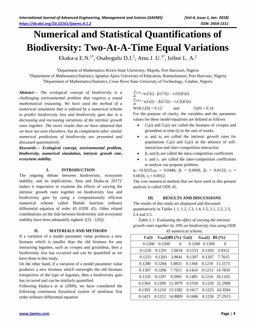
III. RESULTS AND DISCUSSIONS
The results of this study are displayed and discussed
quantitatively in Tables 1.1, 1.2, 1.3, 1.4, 1.5, 2.1, 2.2, 2.3,
2.4 and 2.5.
Table.1.1: Evaluating the effect of varying the intrinsic
growth rates together by 10% on biodiversity loss using ODE
45 numerical scheme.
Cb(t) Cbm(t)BL(%) Gb(t) Gbm(t) BL(%)
0.1200 0.1200 0 0.1200 0.1200 0
0.1226 0.1201 2.0034 0.1253 0.1203 3.9312
0.1253 0.1203 3.9641 0.1307 0.1207 7.7015
0.1280 0.1204 5.8831 0.1364 0.1210 11.3173
0.1307 0.1206 7.7611 0.1424 0.1213 14.7850
0.1335 0.1207 9.5991 0.1485 0.1216 18.1105
0.1364 0.1209 11.3979 0.1550 0.1220 21.2998
0.1393 0.1210 13.1582 0.1617 0.1223 24.3584
0.1423 0.1212 14.8809 0.1686 0.1226 27.2915

International Journal of Advanced Engineering, Management and Science (IJAEMS) [Vol-4, Issue-1, Jan- 2018]
https://dx.doi.org/10.22161/ijaems.4.1.2 ISSN: 2454-1311
www.ijaems.com Page | 5
0.1454 0.1213 16.5668 0.1759 0.1230 30.1044
0.1485 0.1214 18.2166 0.1835 0.1233 32.8018
0.1517 0.1216 19.8310 0.1913 0.1236 35.3886
0.1549 0.1217 21.4108 0.1995 0.1239 37.8693
0.1582 0.1219 22.9568 0.2080 0.1243 40.2481
0.1616 0.1220 24.4695 0.2168 0.1246 42.5293
0.1650 0.1222 25.9497 0.2260 0.1249 44.7168
0.1685 0.1223 27.3980 0.2355 0.1253 46.8144
0.1720 0.1225 28.8152 0.2454 0.1256 48.8258
0.1757 0.1226 30.2018 0.2557 0.1259 50.7546
0.1793 0.1227 31.5585 0.2664 0.1263 52.6041
From Table 1.1, when all the model parameter values are
fixed, the cowpea biomass data denoted Cb(t) when the
length of the growing season is twenty one weeks range from
a low value of 0.12grams/area to 0.1793grams/area whereas
Cbm(t) data range from a low value 0.12 grams/area to 0.1227
grams/area due to a 10% variation of the intrinsic growth
rates together. On the basis of this calculation, the new
simulated cowpea data due to a joint variation of the intrinsic
growth rates dominantly predicts a depletion which mimics
biodiversity loss. The extent of biodiversity loss has been
quantified to range from zero to 31.6 approximately
providing an average of 16.8 which re-classifies the
vulnerability of the cowpea biomass to biodiversity loss. A
similar observation can be made from the groundnut biomass
component. In summary, the groundnut biomass is about
1.67 approximately more vulnerable to biodiversity loss than
the cowpea biomass. Statistically, the average of biomass
vulnerability to biodiversity loss with respect to the
groundnut legume is 29.57% approximately.
Table.1.2: Evaluating the effect of varying the intrinsic
growth rates together by 15% on biodiversity loss using ODE
45 numerical scheme.
Cb(t) Cbm(t)BL(%) Gb(t) Gbm(t) BL(%)
0.1200 0.1200 0 0.1200 0.1200 0
0.1226 0.1203 1.8931 0.1253 0.1206 3.7169
0.1253 0.1206 3.7480 0.1307 0.1212 7.2896
0.1280 0.1208 5.5655 0.1364 0.1218 10.7235
0.1307 0.1211 7.3462 0.1424 0.1224 14.0240
0.1335 0.1214 9.0908 0.1485 0.1230 17.1963
0.1364 0.1217 10.8001 0.1550 0.1236 20.2451
0.1393 0.1220 12.4747 0.1617 0.1242 23.1754
0.1423 0.1222 14.1153 0.1686 0.1248 25.9917
0.1454 0.1225 15.7226 0.1759 0.1254 28.6983
0.1485 0.1228 17.2972 0.1835 0.1260 31.2995
0.1517 0.1231 18.8398 0.1913 0.1267 33.7993
0.1549 0.1234 20.3509 0.1995 0.1273 36.2017
0.1582 0.1237 21.8312 0.2080 0.1279 38.5104
0.1616 0.1239 23.2813 0.2168 0.1285 40.7289
0.1650 0.1242 24.7017 0.2260 0.1291 42.8609
0.1685 0.1245 26.0930 0.2355 0.1298 44.9095
0.1720 0.1248 27.4558 0.2454 0.1304 46.8781
0.1757 0.1251 28.7906 0.2557 0.1310 48.7696
0.1793 0.1254 30.0981 0.2664 0.1316 50.5872
From Table 1.2, when all the model parameter values are
fixed, the cowpea biomass data denoted Cb(t) when the
length of the growing season is twenty one weeks range from
a low value of 0.12 grams/area to 0.1793 grams/area whereas
Cbm(t) data range from a low value 0.12 grams/area to 0.1254
grams/area due to a 15% variation of the intrinsic growth
rates together. On the basis of this calculation, the new
simulated cowpea data due to a joint variation of the intrinsic
growth rates dominantly predicts a depletion which mimics
biodiversity loss. The extent of biodiversity loss has been
quantified to range from zero to 30.1 approximately
providing an average of 15.97 which re-classifies the
vulnerability of the cowpea biomass to biodiversity loss. A
similar observation can be made from the groundnut biomass
component. In summary, the groundnut biomass is about
1.68 approximately more vulnerable to biodiversity loss than
the cowpea biomass. Statistically, the average of biomass
vulnerability to biodiversity loss with respect to the
groundnut legume is 28.28% approximately.
Table.1.3: Evaluating the effect of varying the intrinsic
growth rates together by 20% on biodiversity loss using ODE
45 numerical scheme.
Cb(t) Cbm(t)BL(%) Gb(t) Gbm(t) BL(%)
0.1200 0.1200 0 0.1200 0.1200 0
0.1226 0.1204 1.7828 0.1253 0.1209 3.5022
0.1253 0.1208 3.5315 0.1307 0.1217 6.8759
0.1280 0.1212 5.2468 0.1364 0.1226 10.1258
0.1307 0.1217 6.9293 0.1424 0.1235 13.2563
0.1335 0.1221 8.5796 0.1485 0.1244 16.2718
0.1364 0.1225 10.1982 0.1550 0.1253 19.1764
0.1393 0.1229 11.7858 0.1617 0.1261 21.9741
0.1423 0.1233 13.3429 0.1686 0.1270 24.6688
0.1454 0.1238 14.8699 0.1759 0.1279 27.2641
0.1485 0.1242 16.3676 0.1835 0.1289 29.7638

International Journal of Advanced Engineering, Management and Science (IJAEMS) [Vol-4, Issue-1, Jan- 2018]
https://dx.doi.org/10.22161/ijaems.4.1.2 ISSN: 2454-1311
www.ijaems.com Page | 6
0.1517 0.1246 17.8364 0.1913 0.1298 32.1712
0.1549 0.1250 19.2768 0.1995 0.1307 34.4897
0.1582 0.1255 20.6893 0.2080 0.1316 36.7225
0.1616 0.1259 22.0745 0.2168 0.1325 38.8727
0.1650 0.1263 23.4328 0.2260 0.1335 40.9432
0.1685 0.1267 24.7647 0.2355 0.1344 42.9371
0.1720 0.1272 26.0707 0.2454 0.1353 44.8570
0.1757 0.1276 27.3513 0.2557 0.1363 46.7055
0.1793 0.1280 28.6068 0.2664 0.1372 48.4854
From Table 1.3, when all the model parameter values are
fixed, the cowpea biomass data Cb(t) when the length of the
growing season is twenty one weeks range from a low value
of 0.12 grams/area to 0.1793 grams/area whereas Cbm(t) data
range from a low value 0.12 grams/area to 0.1280 grams/area
due to a 20% variation of the intrinsic growth rates together.
On the basis of this calculation, the new simulated cowpea
data due to a joint variation of the intrinsic growth rates
dominantly predicts a depletion which mimics biodiversity
loss. The extent of biodiversity loss has been quantified to
range from zero to 28.6 approximately providing an average
of 15.14 which re-classifies the vulnerability of the cowpea
biomass to biodiversity loss. A similar observation can be
made from the groundnut biomass component. In summary,
the groundnut biomass is about 1.69 approximately more
vulnerable to biodiversity loss than the cowpea biomass.
Statistically, the average of biomass vulnerability to
biodiversity loss with respect to the groundnut legume is
26.95% approximately.
Table.1.4: Evaluating the effect of varying the intrinsic
growth rates together by 25% on biodiversity loss using ODE
45 numerical scheme.
Cb(t) Cbm(t)BL(%) Gb(t) Gbm(t) BL(%)
0.1200 0.1200 0 0.1200 0.1200 0
0.1226 0.1206 1.6723 0.1253 0.1211 3.2869
0.1253 0.1211 3.3145 0.1307 0.1223 6.4603
0.1280 0.1217 4.9271 0.1364 0.1234 9.5240
0.1307 0.1222 6.5106 0.1424 0.1246 12.4818
0.1335 0.1228 8.0656 0.1485 0.1258 15.3370
0.1364 0.1233 9.5924 0.1550 0.1269 18.0933
0.1393 0.1239 11.0915 0.1617 0.1281 20.7540
0.1423 0.1245 12.5635 0.1686 0.1293 23.3223
0.1454 0.1250 14.0087 0.1759 0.1305 25.8013
0.1485 0.1256 15.4276 0.1835 0.1317 28.1940
0.1517 0.1262 16.8207 0.1913 0.1330 30.5033
0.1549 0.1267 18.1883 0.1995 0.1342 32.7321
0.1582 0.1273 19.5309 0.2080 0.1354 34.8830
0.1616 0.1279 20.8489 0.2168 0.1367 36.9588
0.1650 0.1284 22.1427 0.2260 0.1379 38.9619
0.1685 0.1290 23.4128 0.2355 0.1392 40.8947
0.1720 0.1296 24.6594 0.2454 0.1405 42.7597
0.1757 0.1302 25.8831 0.2557 0.1418 44.5592
0.1793 0.1308 27.0841 0.2664 0.1431 46.2954
Table.1.5: Evaluating the effect of varying the intrinsic
growth rates together by 95% on biodiversity loss using ODE
45 numerical scheme.
Cb(t) Cbm(t)BL(%) Gb(t) Gbm(t) BL(%)
0.1200 0.1200 0 0.1200 0.1200 0
0.1226 0.1225 0.1124 0.1253 0.1250 0.2226
0.1253 0.1250 0.2245 0.1307 0.1301 0.4442
0.1280 0.1275 0.3363 0.1364 0.1355 0.6650
0.1307 0.1301 0.4478 0.1424 0.1411 0.8847
0.1335 0.1328 0.5590 0.1485 0.1469 1.1035
0.1364 0.1355 0.6699 0.1550 0.1529 1.3213
0.1393 0.1383 0.7805 0.1617 0.1592 1.5381
0.1423 0.1411 0.8908 0.1686 0.1657 1.7537
0.1454 0.1439 1.0007 0.1759 0.1724 1.9682
0.1485 0.1468 1.1103 0.1835 0.1795 2.1815
0.1517 0.1498 1.2195 0.1913 0.1867 2.3936
0.1549 0.1528 1.3284 0.1995 0.1943 2.6045
0.1582 0.1559 1.4369 0.2080 0.2021 2.8141
0.1616 0.1591 1.5450 0.2168 0.2103 3.0223
0.1650 0.1623 1.6527 0.2260 0.2187 3.2291
0.1685 0.1655 1.7600 0.2355 0.2274 3.4344
0.1720 0.1688 1.8668 0.2454 0.2365 3.6383
0.1757 0.1722 1.9733 0.2557 0.2459 3.8406
0.1793 0.1756 2.0792 0.2664 0.2556 4.0412
Table.2.1: Evaluating the effect of varying the intrinsic
growth rates together by 105% on biodiversity gain using
ODE 45 numerical scheme.
Cb(t) Cbm(t)BG(%) Gb(t) Gbm(t) BG(%)
0.1200 0.1200 0 0.1200 0.1200 0
0.1226 0.1227 0.1125 0.1253 0.1255 0.2231
0.1253 0.1255 0.2250 0.1307 0.1313 0.4462
0.1280 0.1284 0.3374 0.1364 0.1373 0.6694
0.1307 0.1313 0.4498 0.1424 0.1436 0.8926
0.1335 0.1343 0.5621 0.1485 0.1502 1.1158
0.1364 0.1373 0.6744 0.1550 0.1570 1.3389

International Journal of Advanced Engineering, Management and Science (IJAEMS) [Vol-4, Issue-1, Jan- 2018]
https://dx.doi.org/10.22161/ijaems.4.1.2 ISSN: 2454-1311
www.ijaems.com Page | 7
0.1393 0.1404 0.7866 0.1617 0.1642 1.5620
0.1423 0.1436 0.8987 0.1686 0.1717 1.7848
0.1454 0.1469 1.0108 0.1759 0.1794 2.0074
0.1485 0.1502 1.1227 0.1835 0.1875 2.2298
0.1517 0.1535 1.2345 0.1913 0.1960 2.4518
0.1549 0.1570 1.3461 0.1995 0.2048 2.6735
0.1582 0.1605 1.4576 0.2080 0.2140 2.8947
0.1616 0.1641 1.5690 0.2168 0.2236 3.1153
0.1650 0.1678 1.6801 0.2260 0.2335 3.3354
0.1685 0.1715 1.7911 0.2355 0.2439 3.5548
0.1720 0.1753 1.9018 0.2454 0.2547 3.7734
0.1757 0.1792 2.0124 0.2557 0.2659 3.9912
0.1793 0.1832 2.1226 0.2664 0.2776 4.2080
Table.2.2: Evaluating the effect of varying the intrinsic
growth rates together by 110% on biodiversity gain using
ODE 45 numerical scheme.
Cb(t) Cbm(t)BG(%) Gb(t) Gbm(t) BG(%)
0.1200 0.1200 0 0.1200 0.1200 0
0.1226 0.1229 0.2251 0.1253 0.1258 0.4466
0.1253 0.1258 0.4504 0.1307 0.1319 0.8944
0.1280 0.1288 0.6759 0.1364 0.1383 1.3433
0.1307 0.1319 0.9016 0.1424 0.1449 1.7932
0.1335 0.1350 1.1274 0.1485 0.1519 2.2441
0.1364 0.1383 1.3533 0.1550 0.1592 2.6958
0.1393 0.1415 1.5794 0.1617 0.1668 3.1482
0.1423 0.1449 1.8055 0.1686 0.1747 3.6013
0.1454 0.1483 2.0317 0.1759 0.1830 4.0549
0.1485 0.1518 2.2578 0.1835 0.1917 4.5089
0.1517 0.1554 2.4840 0.1913 0.2008 4.9632
0.1549 0.1591 2.7102 0.1995 0.2103 5.4177
0.1582 0.1628 2.9363 0.2080 0.2202 5.8722
0.1616 0.1667 3.1623 0.2168 0.2305 6.3265
0.1650 0.1706 3.3881 0.2260 0.2413 6.7804
0.1685 0.1746 3.6138 0.2355 0.2526 7.2339
0.1720 0.1786 3.8393 0.2454 0.2643 7.6867
0.1757 0.1828 4.0646 0.2557 0.2765 8.1387
0.1793 0.1870 4.2895 0.2664 0.2893 8.5895
Table.2.3: Evaluating the effect of varying the intrinsic
growth rates together by 115% on biodiversity gain using
ODE 45 numerical scheme.
Cb(t) Cbm(t)BG(%) Gb(t) Gbm(t) BG(%)
0.1200 0.1200 0 0.1200 0.1200 0
0.1226 0.1230 0.3379 0.1253 0.1261 0.6707
0.1253 0.1261 0.6764 0.1307 0.1325 1.3446
0.1280 0.1293 1.0156 0.1364 0.1392 2.0217
0.1307 0.1325 1.3554 0.1424 0.1462 2.7018
0.1335 0.1358 1.6959 0.1485 0.1536 3.3848
0.1364 0.1392 2.0368 0.1550 0.1613 4.0707
0.1393 0.1427 2.3784 0.1617 0.1694 4.7591
0.1423 0.1462 2.7204 0.1686 0.1778 5.4500
0.1454 0.1498 3.0628 0.1759 0.1867 6.1432
0.1485 0.1536 3.4057 0.1835 0.1960 6.8385
0.1517 0.1574 3.7489 0.1913 0.2057 7.5357
0.1549 0.1612 4.0924 0.1995 0.2159 8.2345
0.1582 0.1652 4.4362 0.2080 0.2266 8.9348
0.1616 0.1693 4.7803 0.2168 0.2377 9.6363
0.1650 0.1734 5.1244 0.2260 0.2494 10.3387
0.1685 0.1777 5.4687 0.2355 0.2615 11.0417
0.1720 0.1820 5.8130 0.2454 0.2743 11.7451
0.1757 0.1865 6.1573 0.2557 0.2875 12.4484
0.1793 0.1910 6.5016 0.2664 0.3014 13.1514
Table.2.4: Evaluating the effect of varying the intrinsic
growth rates together by 120% on biodiversity gain using
ODE 45 numerical scheme.
Cb(t) Cbm(t)BG(%) Gb(t) Gbm(t) BG(%)
0.1200 0.1200 0 0.1200 0.1200 0
0.1226 0.1232 0.4507 0.1253 0.1264 0.8952
0.1253 0.1264 0.9029 0.1307 0.1331 1.7968
0.1280 0.1297 1.3564 0.1364 0.1401 2.7046
0.1307 0.1331 1.8113 0.1424 0.1475 3.6185
0.1335 0.1366 2.2675 0.1485 0.1553 4.5383
0.1364 0.1401 2.7249 0.1550 0.1634 5.4639
0.1393 0.1438 3.1836 0.1617 0.1720 6.3950
0.1423 0.1475 3.6434 0.1686 0.1810 7.3315
0.1454 0.1514 4.1043 0.1759 0.1905 8.2731
0.1485 0.1553 4.5663 0.1835 0.2004 9.2195
0.1517 0.1593 5.0292 0.1913 0.2108 10.1706
0.1549 0.1634 5.4931 0.1995 0.2217 11.1258
0.1582 0.1676 5.9578 0.2080 0.2331 12.0850
0.1616 0.1719 6.4233 0.2168 0.2451 13.0478

International Journal of Advanced Engineering, Management and Science (IJAEMS) [Vol-4, Issue-1, Jan- 2018]
https://dx.doi.org/10.22161/ijaems.4.1.2 ISSN: 2454-1311
www.ijaems.com Page | 8
0.1650 0.1763 6.8895 0.2260 0.2577 14.0138
0.1685 0.1809 7.3564 0.2355 0.2708 14.9825
0.1720 0.1855 7.8237 0.2454 0.2846 15.9536
0.1757 0.1902 8.2915 0.2557 0.2990 16.9265
0.1793 0.1951 8.7597 0.2664 0.3141 17.9007
Table.2.5: Evaluating the effect of varying the intrinsic
growth rates together by 125% on biodiversity gain using
ODE 45 numerical scheme.
Cb(t) Cbm(t)BG(%) Gb(t) Gbm(t) BG(%)
0.1200 0.1200 0 0.1200 0.1200 0
0.1226 0.1233 0.5637 0.1253 0.1267 1.1203
0.1253 0.1267 1.1299 0.1307 0.1337 2.2510
0.1280 0.1301 1.6984 0.1364 0.1410 3.3921
0.1307 0.1337 2.2692 0.1424 0.1488 4.5433
0.1335 0.1373 2.8423 0.1485 0.1570 5.7046
0.1364 0.1411 3.4176 0.1550 0.1656 6.8757
0.1393 0.1449 3.9951 0.1617 0.1747 8.0564
0.1423 0.1488 4.5747 0.1686 0.1842 9.2464
0.1454 0.1529 5.1563 0.1759 0.1943 10.4454
0.1485 0.1570 5.7398 0.1835 0.2048 11.6532
0.1517 0.1613 6.3253 0.1913 0.2159 12.8694
0.1549 0.1656 6.9125 0.1995 0.2276 14.0935
0.1582 0.1701 7.5014 0.2080 0.2399 15.3253
0.1616 0.1746 8.0919 0.2168 0.2527 16.5641
0.1650 0.1793 8.6839 0.2260 0.2662 17.8095
0.1685 0.1841 9.2773 0.2355 0.2804 19.0609
0.1720 0.1890 9.8720 0.2454 0.2953 20.3177
0.1757 0.1940 10.4678 0.2557 0.3109 21.5792
0.1793 0.1992 11.0647 0.2664 0.3273 22.8448
Statistical measure by
Table
BL1
(Average)
BL2
(Average)
Table 1.1 16.801 29.5726
Table 1.2 15.9748 28.2803
Table 1.3 15.1369 26.9532
Table 1.4 14.2872 25.5902
Table 1.5 1.0497 2.0550
Statistical measure by
Table
BG1
(Average)
BG1
(Average)
Table 2.1 1.0648 2.1134
Table 2.2 2.1448 4.2870
Table 2.3 3.2404 6.5226
Table 2.4 4.3518 8.8221
Table 2.5 5.4792 11.1876
IV. CONCLUSION
By using ODE 45 we have found out that a biodiversity loss
can be obtained due to a decreasing variation of the intrinsic
growth rates together, whereas a dominant biodiversity gain
can be obtained due to an increasing variation of the intrinsic
growth rates together. On the basis of this analysis, the
decreasing variation of the intrinsic growth rates together has
generally indicated a decrease in the yields of these two
crops, whereas an increasing variation of the same parameter
values has indicated an improvement in the yields of both
cowpea and groundnut. In this context, an alarming rate of
biodiversity loss of these quantified magnitude are a strong
signal on lower food production, endemic poverty and a
weak sustainable development scenario, whereas a
biodiversity gain has the potential to alleviate poverty and
sustain development. These two components of biodiversity
as predicted in this work have their policy implications.
This present numerical idea can be extended to examine the
effects of varying the intra and inter competition coefficients
together in our future investigation.
REFERENCES
[1] Atsu, J. U. & Ekaka-a, E. N. (2017). Modeling the
policy implications of biodiversity loss: A case study of
the Cross River national park, south – south Nigeria.
International Journal of Pure and Applied Science,
Cambridge Research and Publications. vol 10 No. 1; pp
30-37.
[2] Atsu, J. U. & Ekaka-a, E. N. (2017). Quantifying the
impact of changing intrinsic growth rate on the
biodiversity of the forest resource biomass: implications
for the Cross River State forest resource at the Cross
River National Park, South – South, Nigeria: African
Scholar Journal of Pure and Applied Science, 7(1); 117
– 130.
[3] De Mazancourt, C., Isbell, F., Larocque, A., Berendse,
F., De Luca, E., Grace,J.B etal. (2013). Predicting
ecosystem stability from community composition and
biodiversity. Ecology Letters,, DOI: 10.1111/ele.12088.
[4] Doak, D.F., Bigger, D., Harding, E.K., Marvier, M.A.,
O’Malley, R.E. &Thomson, D. (1998). The statistical
inevitability of stability-diversity relationships in
community ecology. Am. Nat., 151, 264–276.
[5] Ernest, S.K.M. & Brown, J.H. (2001).Homeostasis and
compensation: the roleof species and resources in
ecosystem stability. Ecology, 82, 2118–2132.Fowler,
M.S. (2009). Increasing community size and
connectance can increase stability in competitive
communities. J. Theor. Biol., 258, 179–188.
[6] Fowler, M.S., Laakso, J., Kaitala, V., Ruokolainen, L.
& Ranta, E. (2012). Species dynamics alter community

International Journal of Advanced Engineering, Management and Science (IJAEMS) [Vol-4, Issue-1, Jan- 2018]
https://dx.doi.org/10.22161/ijaems.4.1.2 ISSN: 2454-1311
www.ijaems.com Page | 9
diversity-biomass stability relationships. Ecol. Lett.,15,
1387–1396.
[7] Gonzalez, A. & Descamps-Julien, B. (2004). Population
and community variability in randomly fluctuating
environments. Oikos, 106, 105–116.
[8] Gonzalez, A. & Loreau, M. (2009). The causes and
consequences of compensatory dynamics in ecological
communities. Annu. Rev. Ecol. Evol. Syst., 40, 393–
414.
[9] Grman, E., Lau, J.A., Donald, R., Schoolmaster, J. &
Gross, K.L. (2010).Mechanisms contributing to stability
in ecosystem function depend on the environmental
context. Ecol. Lett., 13, 1400–1410.
[10] Hector, A., Hautier, Y., Saner, P., Wacker, L., Bagchi,
R., Joshi, J. et al. (2010).General stabilizing effects of
plant diversity on grassland productivity through
population asynchrony and over yielding. Ecology, 91,
2213–2220.
[11] Loreau, M.. & de Mazancourt, C.. (2013). Biodiversity
and ecosystem stability: a synthesis of underlying
mechanisms. Ecol. Lett., DOI: 10.1111/ele.12073.
[12] Loreau, M. & Hector, A. (2001). Partitioning selection
and complementarity in biodiversity experiments.
Nature, 412, 72–76.
[13] MacArthur, R. (1955). Fluctuations of Animal
Populations, and a Measure of Community Stability.
Ecology, 36, 533–536.
[14] Marquard, E., Weigelt, A., Roscher, C., Gubsch, M.,
Lipowsky, A. & Schmid, B.(2009). Positive
biodiversity-productivity relationship due to increased
plant density. J. Ecol., 97, 696–704.
[15] May, R.M. (1973). Stability and complexity in model
ecosystems. 2001, Princeton Landmarks in Biology
edn. Princeton University Press, Princeton. McCann,
K.S. (2000). The diversity-stability debate. Nature, 405,
228–233.
[16] McNaughton, S.J. (1977). Diversity and stability of
ecological communities: a comment on the role of
empiricism in ecology. Am. Nat., 111, 515–525.
[17] Mutshinda, C.M., O’Hara, R.B. & Woiwod, I.P. (2009).
What drives community dynamics? Proc. Biol. Sci.,
276, 2923–2929.
[18] Proulx, R., Wirth, C., Voigt, W., Weigelt, A., Roscher,
C., Attinger, S. et al.(2010). Diversity Promotes
Temporal Stability across Levels of Ecosystem
Organization in Experimental Grasslands. PLoS ONE,
5, e13382.
[19] Roscher, C., Weigelt, A., Proulx, R., Marquard, E.,
Schumacher, J., Weisser, W.W. et al. (2011).
Identifying population- and community-level
mechanisms of diversity–stability relationships in
experimental grasslands. J. Ecol., 99, 1460–1469.
[20] Van Ruijven, J. & Berendse, F. (2007). Contrasting
effects of diversity on the temporal stability of plant
populations. Oikos, 116, 1323–1330.
[21] Solomon, S., D. Qin, M. Manning, Z. Chen, M.
Marquis, K.B. Averyt, M. Tignor and H.L. Miller
(eds.)]. Cambridge University Press, Cambridge, United
Kingdom and New York, NY, USA, 996pp.
[22] Rahmstorf, S., Cazenave, A., Church, J.A., Hansen,
J.E., Keeling, R.F., Parker, D.E., and R.C.J. Somerville,
2007: Recent climate observations compared to
projections. Science 316 (5825):709-709.
[23] Domingues, C.M, Church, J.A:, White, N.J., Gleckler,
P.J, Wijffels, S.E., Barker, P.M. and J.R.Dunn, 2008:.
Improved estimates of upper-ocean warming and multi-
decadal sea-level rise. Nature 453:1090-1094.
International Journal of Advanced Engineering, Management and Science (IJAEMS) [Vol-4, Issue-1, Jan- 2018]
https://dx.doi.org/10.22161/ijaems.4.1.3 ISSN: 2454-1311
www.ijaems.com Page | 10
Modelling the effects of decreasing the inter–
competition coefficients on biodiversity loss Ekaka-a, E. N.1; Eke, Nwagrabe2; Atsu, J. U.3
1Department of Mathematics, Rivers State University Nkporlu–Oroworukwo, Port Harcourt, Rivers State
2Department of Mathematics/Statistics, Ignatius Ajuru University of Education, Port Harcourt, Rivers State 3Department of Mathematics/Statistics, Cross River University of Technology, Calabar, Nigeria.
Abstract— The notion of a biodiversity loss has been
identified as a major devastating biological phenomenon
which needs to be mitigated against. In the short term, we
have utilised a Matlab numerical scheme to quantify the
effects of decreasing and increasing the inter –
competition coefficients on biodiversity loss and
biodiversity gain. On the simplifying assumption of a
fixed initial condition(4, 10), two enhancing factors of
intrinsic growth rates, two inhibiting growth rates of intra
– competition coefficients and two inhibiting growth rates
of inter – competition coefficients. The novel results that
we have obtained; which we have not seen elsewhere
complement our recent contribution to knowledge in the
context of applying a numerical scheme to predict both
biodiversity loss and biodiversity gain.
Keywords— Competition coefficients, biodiversity loss,
biodiversity gain, numerical scheme, initial condition,
intrinsic growth rate.
I. INTRODUCTION
Following the recent application of a numerical
simulation to model biodiversity (Atsu and Ekaka-a
2017), we have come to observe that the mathematical
technique of a numerical simulation which is rarely been
applied to interpret the extent of biodiversity loss and
biodiversity gain is an important short term and long term
quantitative scientific process. We will expect the
application of a numerical simulation to model
biodiversity to contribute to other previous research
outputs.
II. MATERIALS AND METHODS
The core method of ODE 45 numerical scheme has been
coded to analyze a Lotka – Volterra mathematical
structure dynamical system of non – linear first order
differential equation with the following parameter values:
The intrinsic growth rate of the first species is estimated
to be 0.1; the intrinsic growth rate of the second yeast
species is estimated to be 0.08; the intra – competition
coefficients due to the self-interaction between the first
yeast species and itself is estimated to be 0.0014; the intra
– competition coefficients due to the self-interaction
between the second yeast species and itself is estimated to
be 0.001; the intra – competition coefficients which is
another set of inhibiting factors are estimated to be 0.0012
and 0.0009 respectively. The aim of this present analysis
is to vary the inter – competition coefficient together and
quantify the effect of this variation on biodiversity loss
and biodiversity gain in which the initial condition is
specified by (4, 10) for a shorter length of growing
season of twenty (20) days
III. RESULTS
The results of these numerical simulation analyses are
presented in Table 1, Table 2, and Table 3
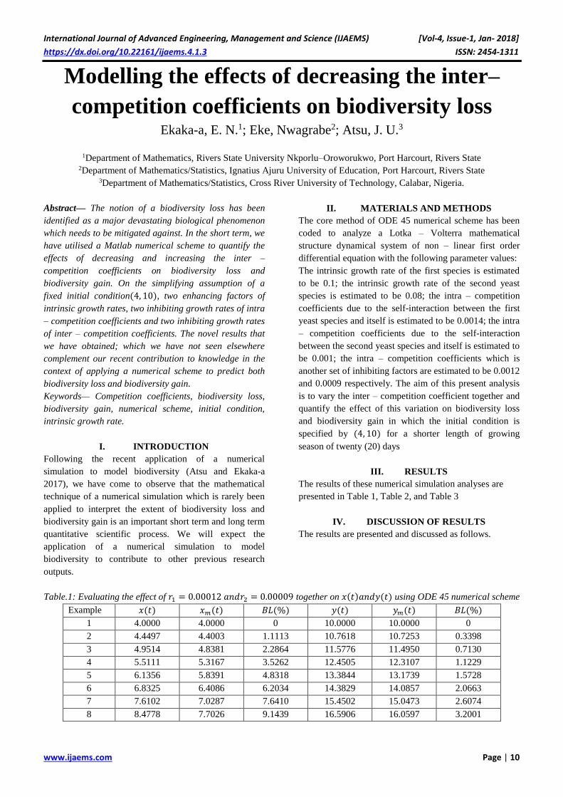
IV. DISCUSSION OF RESULTS
The results are presented and discussed as follows.
Table.1: Evaluating the effect of 𝑟1 = 0.00012 𝑎𝑛𝑑𝑟2 = 0.00009 together on 𝑥(𝑡)𝑎𝑛𝑑𝑦(𝑡) using ODE 45 numerical scheme
Example 𝑥(𝑡) 𝑥𝑚(𝑡) 𝐵𝐿(%) 𝑦(𝑡) 𝑦𝑚(𝑡) 𝐵𝐿(%)
1 4.0000 4.0000 0 10.0000 10.0000 0
2 4.4497 4.4003 1.1113 10.7618 10.7253 0.3398
3 4.9514 4.8381 2.2864 11.5776 11.4950 0.7130
4 5.5111 5.3167 3.5262 12.4505 12.3107 1.1229
5 6.1356 5.8391 4.8318 13.3844 13.1739 1.5728
6 6.8325 6.4086 6.2034 14.3829 14.0857 2.0663
7 7.6102 7.0287 7.6410 15.4502 15.0473 2.6074
8 8.4778 7.7026 9.1439 16.5906 16.0597 3.2001

International Journal of Advanced Engineering, Management and Science (IJAEMS) [Vol-4, Issue-1, Jan- 2018]
https://dx.doi.org/10.22161/ijaems.4.1.3 ISSN: 2454-1311
www.ijaems.com Page | 11
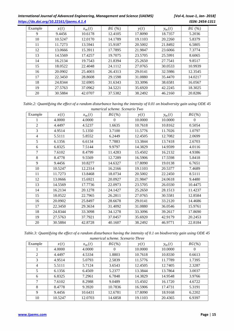
Example 𝑥(𝑡) 𝑥𝑚(𝑡) 𝐵𝐿(%) 𝑦(𝑡) 𝑦𝑚(𝑡) 𝐵𝐿(%)
9 9.4456 8.4339 10.7107 17.8090 17.1235 3.8490
10 10.5247 9.2260 12.3396 19.1103 18.2391 4.5587
11 11.7273 10.0822 14.0278 20.5002 19.4067 5.3340
12 13.0666 11.0058 15.7718 21.9847 20.6261 6.1799
13 14.5569 11.9997 17.5674 23.5705 21.8966 7.1015
14 16.2134 13.0664 19.4097 25.2650 23.2175 8.1041
15 18.0522 14.2084 21.2929 27.0765 24.5875 9.1927
16 20.0902 15.4272 23.2106 29.0141 26.0047 10.3721
17 22.3450 16.7240 25.1557 31.0880 27.4672 11.6469
18 24.8344 18.0991 27.1208 33.3096 28.9723 13.0212
19 27.5763 19.5521 29.0981 35.6920 30.5173 14.4981
20 30.5884 21.0817 31.0794 38.2492 32.0987 16.0800
Table.2: Evaluating the effect of 𝑟1 = 0.00018 𝑎𝑛𝑑𝑟2 = 0.000135 together on 𝑥(𝑡)𝑎𝑛𝑑𝑦(𝑡) using ODE 45 numerical
scheme
Example 𝑥(𝑡) 𝑥𝑚(𝑡) 𝐵𝐿(%) 𝑦(𝑡) 𝑦𝑚(𝑡) 𝐵𝐿(%)
1 4.0000 4.0000 0 10.0000 10.0000 0
2 4.4497 4.4030 1.0500 10.7618 10.7273 0.3210
3 4.9514 4.8443 2.1611 11.5776 11.4995 0.6740
4 5.5111 5.3273 3.3346 12.4505 12.3183 1.0619
5 6.1356 5.8551 4.5715 13.3844 13.1852 1.4881
6 6.8325 6.4313 5.8722 14.3829 14.1015 1.9561
7 7.6102 7.0594 7.2370 15.4502 15.0686 2.4698
8 8.4778 7.7432 8.6654 16.5906 16.0874 3.0332
9 9.4456 8.4862 10.1565 17.8090 17.1588 3.6507
10 10.5247 9.2924 11.7085 19.1103 18.2834 4.3269
11 11.7273 10.1653 13.3193 20.5002 19.4616 5.0665
12 13.0666 11.1085 14.9857 21.9847 20.6932 5.8748
13 14.5569 12.1253 16.7041 23.5705 21.9779 6.7566
14 16.2134 13.2188 18.4699 25.2650 23.3152 7.7174
15 18.0522 14.3916 20.2780 27.0765 24.7040 8.7623
16 20.0902 15.6458 22.1224 29.0141 26.1427 9.8963
17 22.3450 16.9830 23.9966 31.0880 27.6297 11.1241
18 24.8344 18.4039 25.8936 33.3096 29.1626 12.4501
19 27.5763 19.9084 27.8060 35.6920 30.7388 13.8776
20 30.5884 21.4956 29.7263 38.2492 32.3552 15.4095
Table.3: Evaluating the effect of 𝑟1 = 0.001176 𝑎𝑛𝑑𝑟2 = 0.000882 together on 𝑥(𝑡)𝑎𝑛𝑑𝑦(𝑡) using ODE 45 numerical
scheme
Example 𝑥(𝑡) 𝑥𝑚(𝑡) 𝐵𝐿(%) 𝑦(𝑡) 𝑦𝑚(𝑡) 𝐵𝐿(%)
1 4.0000 4.0000 0 10.0000 10.0000 0
2 4.4497 4.4486 0.0249 10.7618 10.7610 0.0076
3 4.9514 4.9488 0.0516 11.5776 11.5757 0.0161
4 5.5111 5.5066 0.0802 12.4505 12.4473 0.0255
5 6.1356 6.1288 0.1108 13.3844 13.3795 0.0361
6 6.8325 6.8227 0.1436 14.3829 14.3760 0.0479
7 7.6102 7.5966 0.1787 15.4502 15.4407 0.0611
8 8.4778 8.4595 0.2161 16.5906 16.5781 0.0759
9 9.4456 9.4214 0.2560 17.8090 17.7925 0.0924
10 10.5247 10.4933 0.2985 19.1103 19.0891 0.1109

International Journal of Advanced Engineering, Management and Science (IJAEMS) [Vol-4, Issue-1, Jan- 2018]
https://dx.doi.org/10.22161/ijaems.4.1.3 ISSN: 2454-1311
www.ijaems.com Page | 12
Example 𝑥(𝑡) 𝑥𝑚(𝑡) 𝐵𝐿(%) 𝑦(𝑡) 𝑦𝑚(𝑡) 𝐵𝐿(%)
11 11.7273 11.6870 0.3437 20.5002 20.4732 0.1316
12 13.0666 13.0155 0.3917 21.9847 21.9507 0.1549
13 14.5569 14.4925 0.4425 23.5705 23.5279 0.1809
14 16.2134 16.1329 0.4964 25.2650 25.2120 0.2101
15 18.0522 17.9523 0.5532 27.0765 27.0108 0.2429
16 20.0902 19.9670 0.6132 29.0141 28.9330 0.2795
17 22.3450 22.1939 0.6763 31.0880 30.9883 0.3206
18 24.8344 24.6499 0.7427 33.3096 33.1875 0.3666
19 27.5763 27.3523 0.8123 35.6920 35.5428 0.4180
20 30.5884 30.3176 0.8852 38.2492 38.0674 0.4753
By using ODE 45 numerical scheme, we have observed
that a ten (10) percent variation of the inter–competition
coefficient has predicted a monotonically increasing
values for the populations ranging from 4.000 to 30.5884
approximately when all the model parameters are fixed.
For the same population, due to a variation of the intrinsic
growth rates, we have obtained a new population of the
first yeast species called 𝑥1(𝑡) ranging from 4.000 to
21.0817. A biodiversity loss has occurred ranging from 0
and increasing monotonically to 31.0794, quantified in
percentage terms. In essence, example twenty (20) shows
that the first yeast population during a shorter growing
season of twenty (20) units of time is more vulnerable to
the ecological risk of biodiversity loss. A similar
observation is applicable to the second yeast species𝑦(𝑡).
In this case, when the model parameter values are fixed,
the simulated growth rate data range from 10.0 and
increased monotonically to 38.2492 compared to the
range from 10.0 to 32.0987 due to a ten (10) percent
variation of the intrinsic growth rates. We have also
observed that biodiversity loss is quantified to range from
0 to 16.08.
In summary, by comparing these two dominant scenarios
of biodiversity loss, it is very clear that the first yeast
species is almost double more vulnerable to biodiversity
loss than the second yeast species. Similar observations
are applicable to Table 2 and Table 3. On the basis of this
analysis, we have observed that a ninety – eight (98)
percent variation of the inter – competition coefficient
together has predicted a far lower volume of biodiversity
loss as expected which can be tolerated because it is an
evidence that this devastating ecological risk will soon be
lost at the next level of variation such as hundred and one
(101) percentage variation.
V. CONCLUSION
We have successfully utilized the technique of ODE 45
numerical scheme to model the possibility of biodiversity
loss. These results have been discussed quantitatively. A
small variation of the inter – competition coefficient
together is dominantly associated with a higher
vulnerability to biodiversity loss whereas the inevitability
of biodiversity loss which should be expected can be
tolerated for a lower decreasing volume of the intrinsic
growth rates together. It is therefore necessary to find
some sort of mitigation measures that will recover
biodiversity loss and sustain biodiversity gain. This idea
will be key subject in our next investigation.
REFERENCES
[1] Atsu, J. U. & Ekaka-a, E. N. (2017). Modeling the
policy implications of biodiversity loss: A case study
of the Cross River national park, south –south
Nigeria. International Journal of Pure and Applied
Science, Cambridge Research and Publications. vol
10 No. 1; pp 30-37.
[2] Atsu, J. U. & Ekaka-a, E. N. (2017). Quantifying the
impact of changing Intrinsic growth rate on the
biodiversity of the forest resource biomass:
implications for the Cross River State forest resource
at the Cross River National Park, South – South,
Nigeria: African Scholar Journal of Pure and
Applied Science, 7(1); 117 – 130.
[3] De Mazancourt, C., Isbell, F., Larocque, A.,
Berendse, F., De Luca, E., Grace, J.B et al. (2013).
Predicting ecosystem stability from community
composition and biodiversity. Ecology Letters,,
DOI: 10.1111/ele.12088.
[4] Ernest, S.K.M. & Brown, J.H. (2001). Homeostasis
and compensation: the role of species and resources
in ecosystem stability. Ecology, 82, 2118–2132.
[5] Fowler, M.S., Laakso, J., Kaitala, V., Ruokolainen,
L. & Ranta, E. (2012).Species dynamics alter
community diversity-biomass stability relationships.
Ecol. Lett., 15, 1387–1396.
[6] Gonzalez, A. & Descamps-Julien, B. (2004).
Population and community variability in randomly
fluctuating environments. Oikos, 106, 105–116.
[7] Grman, E., Lau, J.A., Donald, R., Schoolmaster, J.
& Gross, K.L. (2010). Mechanisms contributing to

International Journal of Advanced Engineering, Management and Science (IJAEMS) [Vol-4, Issue-1, Jan- 2018]
https://dx.doi.org/10.22161/ijaems.4.1.3 ISSN: 2454-1311
www.ijaems.com Page | 13
stability in ecosystem function depend on the
environmental context. Ecol. Lett., 13, 1400–1410.
[8] Hector, A., Hautier, Y., Saner, P., Wacker, L.,
Bagchi, R., Joshi, J. et al. (2010). General stabilizing
effects of plant diversity on grassland productivity
through population asynchrony and overyielding.
Ecology, 91, 2213–2220.
[9] Loreau, M.. & de Mazancourt, C.. (2013).
Biodiversity and ecosystem stability: a synthesis of
underlying mechanisms. Ecol. Lett., DOI:
10.1111/ele.12073.
[10] MacArthur, R. (1955). Fluctuations of Animal
Populations, and a Measure of Community Stability.
Ecology, 36, 533–536.
[11] Marquard, E., Weigelt, A., Roscher, C., Gubsch, M.,
Lipowsky, A. & Schmid, B. (2009). Positive
biodiversity-productivity relationship due to
increased plant density. J. Ecol., 97, 696–704.
[12] May, R.M. (1973). Stability and complexity in
model ecosystems. 2001, Princeton Landmarks in
Biology edn. Princeton University Press, Princeton.
McCann, K.S. (2000). The diversity-stability debate.
Nature, 405, 228–233.
[13] McNaughton, S.J. (1977). Diversity and stability of
ecological communities: a comment on the role of
empiricism in ecology. Am. Nat., 111, 515–525.
[14] Mutshinda, C.M., O’Hara, R.B. & Woiwod, I.P.
(2009). What drives community dynamics? Proc.
Biol. Sci., 276, 2923–2929.
[15] Proulx, R., Wirth, C., Voigt, W., Weigelt, A.,
Roscher, C., Attinger, S. et al.(2010). Diversity
Promotes Temporal Stability across Levels of
Ecosystem Organization in Experimental
Grasslands. PLoS ONE, 5, e13382.

International Journal of Advanced Engineering, Management and Science (IJAEMS) [Vol-4, Issue-1, Jan- 2018]
https://dx.doi.org/10.22161/ijaems.4.1.4 ISSN: 2454-1311
www.ijaems.com Page | 14
Simulation modelling of the effect of a random
disturbance on biodiversity of a mathematical
model of mutualism between two interacting
yeast species Eke, Nwagrabe1; Atsu, J. U.2; Ekaka-a, E. N3
1Department of Mathematics/Statistics, Ignatius Ajuru University of Education, Port Harcourt, Rivers State
2Department of Mathematics/Statistics, Cross River University of Technology, Calabar, Nigeria. 3Department of Mathematics, Rivers State University Nkporlu–Oroworukwo, Port Harcourt, Rivers State
Abstract— The effect of a random disturbance on the
ecosystem is one of the oldest scientific observations of
which its effect on biodiversity is no exception. We have
used ODE 45 numerical scheme to tackle this problem.
The novel results that we have obtained have not been
seen elsewhere; these are presented and fully discussed
quantitatively.
Keywords— Random disturbance, numerical scheme,
biodiversity, dynamical system, stochastic, deterministic
dynamical system.
I. INTRODUCTION
An ecological dynamical system is inherently stochastic
in its scientific construction and definition. In this
scenario, a deterministic definition of an ecological
dynamical system is a special case of a stochastic
ecological system that is more highly vulnerable to
random disturbance which can be attributed to the other
environmental and climatic factors and other
characteristics of the ecosystem which we cannot go into
in detailed discussion. However, there are two factors that
may have a high potential to influence the performance of
biodiversity gain. One of these factors could be a
conducive steady environment that is less hostile to
interaction between yeast populations. The other factor
could be attributed to an ecological system where human
activities do not have a huge impact on the growing yeast
species. These two factors put together are capable to
improve the performance of yeast species in terms of their
yields that can mimic strong evidence of biodiversity
gain. In other words, a random noise disturbance in terms
of these mentioned factors may not necessarily bring
about biodiversity loss but are capable to increase the
magnitude of biodiversity gain.
II. MATERIALS AND METHODS
We have considered a semi – stochastic fashion of our
deterministic dynamical system in which a dynamical
system with two random noise perturbation scenarios of
0.01 and 0.1 in the first instance and next for a random
noise perturbation of 0.8. This method is based on the 150
percent variation of the inter-competition coefficients
together.
III. RESULTS
The corresponding results of this study are presented in
Table 1, Table 2, Table 3, Table 4, Table 5, and Table 6
Table.1: Quantifying the effect of a random disturbance having the intensity of 0.01 on biodiversity gain using ODE 45
numerical scheme. Scenario One
Example 𝑥(𝑡) 𝑥𝑚(𝑡) 𝐵𝐺 (%) 𝑦(𝑡) 𝑦𝑚(𝑡) 𝐵𝐺 (%)
1 4.0000 4.0000 0 10.0000 10.0000 0
2 4.4497 4.5132 1.4276 10.7618 10.8509 0.8273
3 4.9514 5.1133 3.2706 11.5776 11.7320 1.3340
4 5.5111 5.7691 4.6831 12.4505 12.6952 1.9650
5 6.1356 6.5317 6.4556 13.3844 13.7425 2.6755
6 6.8325 7.3519 7.6024 14.3829 14.8480 3.2337
7 7.6102 8.2747 8.7320 15.4502 16.0596 3.9444
8 8.4778 9.3598 10.4040 16.5906 17.3229 4.4139
International Journal of Advanced Engineering, Management and Science (IJAEMS) [Vol-4, Issue-1, Jan- 2018]
https://dx.doi.org/10.22161/ijaems.4.1.4 ISSN: 2454-1311
www.ijaems.com Page | 15
Example 𝑥(𝑡) 𝑥𝑚(𝑡) 𝐵𝐺 (%) 𝑦(𝑡) 𝑦𝑚(𝑡) 𝐵𝐺 (%)
9 9.4456 10.6178 12.4105 17.8090 18.7357 5.2036
10 10.5247 12.0170 14.1789 19.1103 20.2260 5.8379
11 11.7273 13.5941 15.9187 20.5002 21.8492 6.5805
12 13.0666 15.3911 17.7895 21.9847 23.6066 7.3774
13 14.5569 17.4257 19.7075 23.5705 25.5991 8.6065
14 16.2134 19.7543 21.8394 25.2650 27.7541 9.8517
15 18.0522 22.4048 24.1112 27.0765 30.0533 10.9939
16 20.0902 25.4003 26.4313 29.0141 32.5986 12.3545
17 22.3450 28.8608 29.1598 31.0880 35.4470 14.0217
18 24.8344 32.6905 31.6343 33.3096 38.6581 16.0567
19 27.5763 37.0962 34.5221 35.6920 42.2245 18.3025
20 30.5884 42.0707 37.5382 38.2492 46.2160 20.8286
Table.2: Quantifying the effect of a random disturbance having the intensity of 0.01 on biodiversity gain using ODE 45
numerical scheme. Scenario Two
Example 𝑥(𝑡) 𝑥𝑚(𝑡) 𝐵𝐺(%) 𝑦(𝑡) 𝑦𝑚(𝑡) 𝐵𝐺(%)
1 4.0000 4.0000 0 10.0000 10.0000 0
2 4.4497 4.5237 1.6635 10.7618 10.8162 0.5054
3 4.9514 5.1350 3.7100 11.5776 11.7026 1.0797
4 5.5111 5.8552 6.2449 12.4505 12.7082 2.0699
5 6.1356 6.6134 7.7883 13.3844 13.7418 2.6703
6 6.8325 7.5144 9.9797 14.3829 14.9599 4.0116
7 7.6102 8.4799 11.4283 15.4502 16.2132 4.9386
8 8.4778 9.5569 12.7289 16.5906 17.5598 5.8418
9 9.4456 10.8277 14.6327 17.8090 19.0138 6.7651
10 10.5247 12.2314 16.2166 19.1103 20.5377 7.4689
11 11.7273 13.8468 18.0734 20.5002 22.2450 8.5111
12 13.0666 15.6921 20.0927 21.9847 24.0618 9.4480
13 14.5569 17.7736 22.0973 23.5705 26.0330 10.4475
14 16.2134 20.1278 24.1427 25.2650 28.1513 11.4237
15 18.0522 22.7965 26.2811 27.0765 30.5581 12.8584
16 20.0902 25.8497 28.6678 29.0141 33.2120 14.4686
17 22.3450 29.3634 31.4092 31.0880 36.0546 15.9761
18 24.8344 33.3098 34.1278 33.3096 39.2617 17.8690
19 27.5763 37.7921 37.0457 35.6920 42.9179 20.2453
20 30.5884 42.8728 40.1607 38.2492 46.9771 22.8184
Table.3: Quantifying the effect of a random disturbance having the intensity of 0.1 on biodiversity gain using ODE 45
numerical scheme. Scenario Three
Example 𝑥(𝑡) 𝑥𝑚(𝑡) 𝐵𝐺(%) 𝑦(𝑡) 𝑦𝑚(𝑡) 𝐵𝐺(%)
1 4.0000 4.0000 0 10.0000 10.0000 0
2 4.4497 4.5334 1.8803 10.7618 10.8330 0.6613
3 4.9514 5.0793 2.5839 11.5776 11.7789 1.7395
4 5.5111 5.7124 3.6543 12.4505 12.7405 2.3287
5 6.1356 6.4569 5.2377 13.3844 13.7864 3.0037
6 6.8325 7.2961 6.7848 14.3829 14.9548 3.9766
7 7.6102 8.2988 9.0489 15.4502 16.1720 4.6722
8 8.4778 9.3920 10.7836 16.5906 17.4731 5.3191
9 9.4456 10.6431 12.6781 17.8090 18.9168 6.2202
10 10.5247 12.0703 14.6858 19.1103 20.4365 6.9397

International Journal of Advanced Engineering, Management and Science (IJAEMS) [Vol-4, Issue-1, Jan- 2018]
https://dx.doi.org/10.22161/ijaems.4.1.4 ISSN: 2454-1311
www.ijaems.com Page | 16
Example 𝑥(𝑡) 𝑥𝑚(𝑡) 𝐵𝐺(%) 𝑦(𝑡) 𝑦𝑚(𝑡) 𝐵𝐺(%)
11 11.7273 13.6683 16.5511 20.5002 22.1251 7.9260
12 13.0666 15.4880 18.5308 21.9847 23.9678 9.0203
13 14.5569 17.4978 20.2024 23.5705 25.9385 10.0464
14 16.2134 19.8987 22.7301 25.2650 28.1712 11.5028
15 18.0522 22.5636 24.9908 27.0765 30.5360 12.7766
16 20.0902 25.5495 27.1740 29.0141 33.1085 14.1121
17 22.3450 28.9518 29.5672 31.0880 36.0206 15.8668
18 24.8344 32.8223 32.1648 33.3096 39.2187 17.7398
19 27.5763 37.2030 34.9093 35.6920 42.7775 19.8519
20 30.5884 42.1760 37.8825 38.2492 46.7649 22.2637
Table.4: Quantifying the effect of a random disturbance having the intensity of 0.1 on biodiversity gain using ODE 45
numerical scheme. Scenario Four
Example 𝑥(𝑡) 𝑥𝑚(𝑡) 𝐵𝐺(%) 𝑦(𝑡) 𝑦𝑚(𝑡) 𝐵𝐺(%)
1 4.0000 4.0000 0 10.0000 10.0000 0
2 4.4497 4.4867 0.8312 10.7618 10.8039 0.3907
3 4.9514 5.0647 2.2898 11.5776 11.6835 0.9150
4 5.5111 5.6951 3.3405 12.4505 12.6824 1.8624
5 6.1356 6.5067 6.0488 13.3844 13.7450 2.6946
6 6.8325 7.3949 8.2316 14.3829 14.8654 3.3550
7 7.6102 8.3792 10.1059 15.4502 16.0553 3.9163
8 8.4778 9.4514 11.4848 16.5906 17.3531 4.5954
9 9.4456 10.7237 13.5309 17.8090 18.7569 5.3224
10 10.5247 12.1772 15.7008 19.1103 20.2479 5.9526
11 11.7273 13.7391 17.1551 20.5002 21.9514 7.0789
12 13.0666 15.5557 19.0486 21.9847 23.7044 7.8224
13 14.5569 17.6162 21.0155 23.5705 25.6845 8.9686
14 16.2134 19.9303 22.9250 25.2650 27.9186 10.5029
15 18.0522 22.5407 24.8641 27.0765 30.2741 11.8094
16 20.0902 25.5231 27.0421 29.0141 32.9389 13.5275
17 22.3450 28.9112 29.3857 31.0880 35.7840 15.1058
18 24.8344 32.8304 32.1974 33.3096 38.9832 17.0329
19 27.5763 37.2158 34.9561 35.6920 42.5658 19.2588
20 30.5884 42.1994 37.9592 38.2492 46.5714 21.7578
Table.5: Quantifying the effect of a random disturbance having the intensity of 0.8 on biodiversity gain using ODE 45
numerical scheme. Scenario Five
Example 𝑥(𝑡) 𝑥𝑚(𝑡) 𝐵𝐺(%) 𝑦(𝑡) 𝑦𝑚(𝑡) 𝐵𝐺(%)
1 4.0000 4.0000 0 10.0000 10.0000 0
2 4.4497 4.8324 8.6014 10.7618 11.4308 6.2161
3 4.9514 5.8134 17.4109 11.5776 12.7359 10.0048
4 5.5111 6.9156 25.4863 12.4505 14.2481 14.4378
5 6.1356 8.2866 35.0587 13.3844 15.5423 16.1229
6 6.8325 9.6980 41.9400 14.3829 17.1956 19.5561
7 7.6102 11.2228 47.4713 15.4502 18.8135 21.7691
8 8.4778 12.9207 52.4067 16.5906 20.7384 25.0008
9 9.4456 15.1202 60.0765 17.8090 22.8115 28.0896
10 10.5247 17.3165 64.5317 19.1103 25.0589 31.1277
11 11.7273 19.9405 70.0344 20.5002 27.5825 34.5477
12 13.0666 22.7270 73.9314 21.9847 30.4937 38.7040
International Journal of Advanced Engineering, Management and Science (IJAEMS) [Vol-4, Issue-1, Jan- 2018]
https://dx.doi.org/10.22161/ijaems.4.1.4 ISSN: 2454-1311
www.ijaems.com Page | 17
Example 𝑥(𝑡) 𝑥𝑚(𝑡) 𝐵𝐺(%) 𝑦(𝑡) 𝑦𝑚(𝑡) 𝐵𝐺(%)
13 14.5569 26.0227 78.7651 23.5705 33.5233 42.2257
14 16.2134 29.7098 83.2424 25.2650 36.7004 45.2614
15 18.0522 34.0788 88.7790 27.0765 40.6045 49.9621
16 20.0902 39.0831 94.5379 29.0141 44.6849 54.0111
17 22.3450 44.9096 100.9828 31.0880 48.9859 57.5719
18 24.8344 51.3077 106.5995 33.3096 53.9942 62.0979
19 27.5763 58.3908 111.7429 35.6920 60.0885 68.3532
20 30.5884 66.7729 118.2950 38.2492 66.8022 74.6498
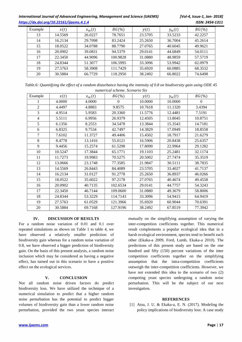
Table.6: Quantifying the effect of a random disturbance having the intensity of 0.8 on biodiversity gain using ODE 45
numerical scheme. Scenario Six
Example 𝑥(𝑡) 𝑥𝑚(𝑡) 𝐵𝐺(%) 𝑦(𝑡) 𝑦𝑚(𝑡) 𝐵𝐺(%)
1 4.0000 4.0000 0 10.0000 10.0000 0
2 4.4497 4.8883 9.8575 10.7618 11.1320 3.4394
3 4.9514 5.9583 20.3360 11.5776 12.4481 7.5191
4 5.5111 6.9956 26.9379 12.4505 13.8045 10.8751
5 6.1356 8.2553 34.5478 13.3844 15.3543 14.7181
6 6.8325 9.7534 42.7497 14.3829 17.0949 18.8558
7 7.6102 11.3727 49.4406 15.4502 18.7917 21.6279
8 8.4778 13.1416 55.0121 16.5906 20.8438 25.6357
9 9.4456 15.2574 61.5298 17.8090 22.9964 29.1282
10 10.5247 17.3844 65.1771 19.1103 25.2481 32.1174
11 11.7273 19.9983 70.5275 20.5002 27.7474 35.3519
12 13.0666 23.1748 77.3585 21.9847 30.5111 38.7835
13 14.5569 26.8443 84.4089 23.5705 33.4027 41.7137
14 16.2134 31.0127 91.2778 25.2650 36.8937 46.0266
15 18.0522 35.6022 97.2178 27.0765 40.4674 49.4558
16 20.0902 40.7135 102.6534 29.0141 44.7757 54.3243
17 22.3450 46.7144 109.0600 31.0880 49.3679 58.8006
18 24.8344 53.3229 114.7143 33.3096 54.9415 64.9419
19 27.5763 61.0529 121.3966 35.6920 60.9044 70.6391
20 30.5884 69.7168 127.9196 38.2492 67.8519 77.3942
IV. DISCUSSION OF RESULTS
For a random noise variation of 0.01 and 0.1 over
repeated simulations as shown on Table 1 to table 4, we
have observed a relatively smaller prediction of
biodiversity gain whereas for a random noise variation of
0.8, we have observed a bigger prediction of biodiversity
gain. On the basis of this present analysis, a random noise
inclusion which may be considered as having a negative
effect, has turned out in this scenario to have a positive
effect on the ecological services.
V. CONCLUSION
Not all random noise driven factors do predict
biodiversity loss. We have utilized the technique of a
numerical simulation to predict that a higher random
noise perturbation has the potential to predict bigger
volumes of biodiversity gain than a lower random noise
perturbation, provided the two yeast species interact
mutually on the simplifying assumption of varying the
inter-competition coefficients together. This numerical
result complements a popular ecological idea that in a
harsh ecological environment, species tend to benefit each
other (Ekaka-a 2009, Ford, Lumb, Ekaka-a 2010). The
predictions of this present study are based on the one
hundred and fifty (150) percent variations of the inter
competition coefficients together on the simplifying
assumption that the intra-competition coefficients
outweigh the inter-competition coefficients. However, we
have not extended this idea to the scenario of two (2)
competing yeast species undergoing a random noise
perturbation. This will be the subject of our next
investigation.
REFERENCES
[1] Atsu, J. U. & Ekaka-a, E. N. (2017). Modeling the
policy implications of biodiversity loss: A case study

International Journal of Advanced Engineering, Management and Science (IJAEMS) [Vol-4, Issue-1, Jan- 2018]
https://dx.doi.org/10.22161/ijaems.4.1.4 ISSN: 2454-1311
www.ijaems.com Page | 18
of the Cross River national park, south – south
Nigeria. International Journal of Pure and Applied
Science, Cambridge Research and Publications. vol
10 No. 1; pp 30-37.
[2] Atsu, J. U. & Ekaka-a, E. N. (2017). Quantifying the
impact of changing intrinsic growth rate on the
biodiversity of the forest resource biomass:
implications for the Cross River State forest resource
at the Cross River National Park, South – South,
Nigeria: African Scholar Journal of Pure and
Applied Science, 7(1); 117 – 130.
[3] De Mazancourt, C., Isbell, F., Larocque, A.,
Berendse, F., De Luca, E., Grace, J.B et al. (2013).
Predicting ecosystem stability from community
composition and biodiversity. Ecology Letters,,
DOI: 10.1111/ele.12088.
[4] Ernest, S.K.M. & Brown, J.H. (2001). Homeostasis
and compensation: the role of species and resources
in ecosystem stability. Ecology, 82, 2118–2132.
[5] Fowler, M.S., Laakso, J., Kaitala, V., Ruokolainen,
L. & Ranta, E. (2012). Species dynamics alter
community diversity-biomass stability relationships.
Ecol. Lett., 15, 1387–1396.
[6] Gonzalez, A. & Descamps-Julien, B. (2004).
Population and community variability in randomly
fluctuating environments. Oikos, 106, 105–116.
[7] Grman, E., Lau, J.A., Donald, R., Schoolmaster, J.
& Gross, K.L. (2010). Mechanisms contributing to
stability in ecosystem function depend on the
environmental context. Ecol. Lett., 13, 1400–1410.
[8] Hector, A., Hautier, Y., Saner, P., Wacker, L.,
Bagchi, R., Joshi, J. et al. (2010). General stabilizing
effects of plant diversity on grassland productivity
through population asynchrony and overyielding.
Ecology, 91, 2213–2220.
[9] Loreau, M.. & de Mazancourt, C.. (2013).
Biodiversity and ecosystem stability: a synthesis of
underlying mechanisms. Ecol. Lett., DOI:
10.1111/ele.12073.
[10] MacArthur, R. (1955). Fluctuations of Animal
Populations, and a Measure of Community Stability.
Ecology, 36, 533–536.
[11] Marquard, E., Weigelt, A., Roscher, C., Gubsch, M.,
Lipowsky, A. & Schmid, B. (2009). Positive
biodiversity-productivity relationship due to
increased plant density. J. Ecol., 97, 696–704.
[12] May, R.M. (1973). Stability and complexity in
model ecosystems. 2001, Princeton Landmarks in
Biology edn. Princeton University Press, Princeton.
McCann, K.S. (2000). The diversity-stability debate.
Nature, 405, 228–233.
[13] McNaughton, S.J. (1977). Diversity and stability of
ecological communities: a comment on the role of
empiricism in ecology. Am. Nat., 111, 515–525.
[14] Mutshinda, C.M., O’Hara, R.B. & Woiwod, I.P.
(2009). What drives community dynamics? Proc.
Biol. Sci., 276, 2923–2929.
[15] Proulx, R., Wirth, C., Voigt, W., Weigelt, A.,
Roscher, C., Attinger, S. et al.(2010). Diversity
Promotes Temporal Stability across Levels of
Ecosystem Organization in Experimental
Grasslands. PLoS ONE, 5, e13382.
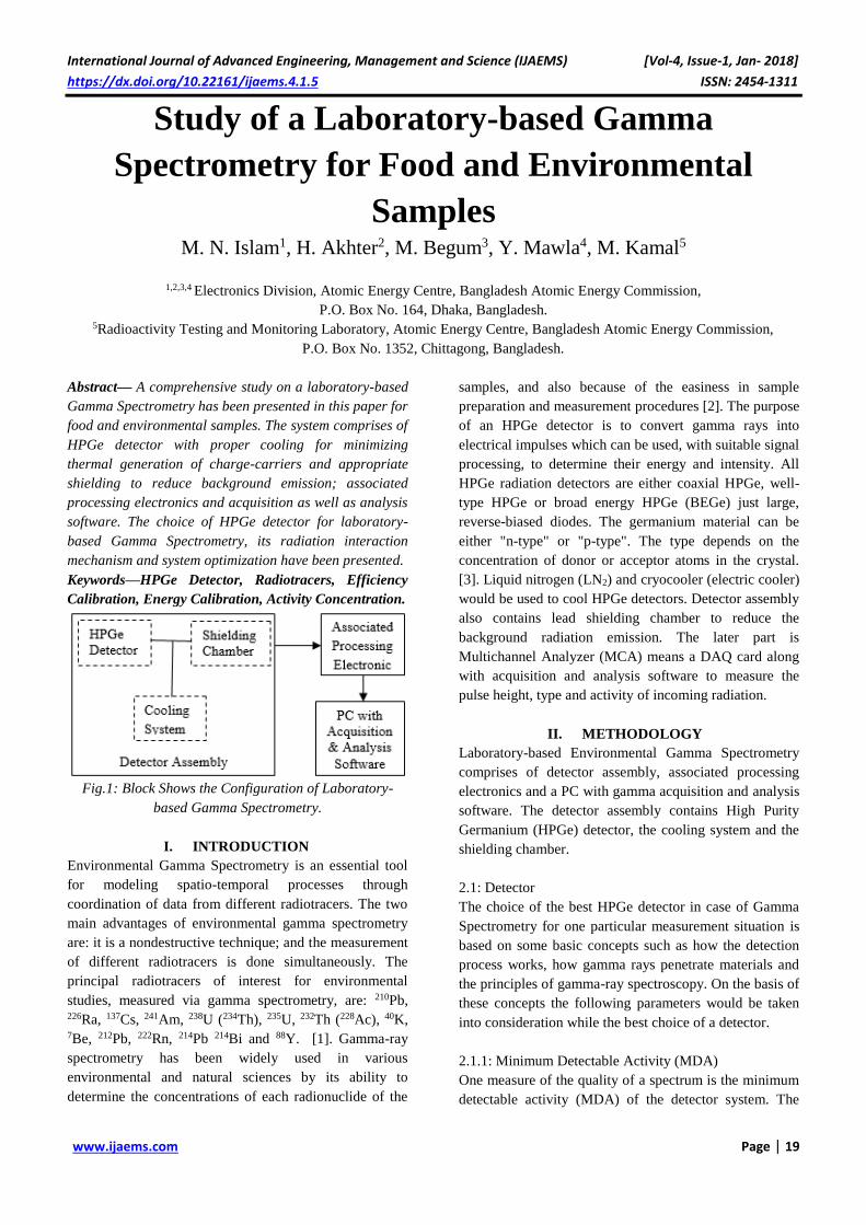
International Journal of Advanced Engineering, Management and Science (IJAEMS) [Vol-4, Issue-1, Jan- 2018]
https://dx.doi.org/10.22161/ijaems.4.1.5 ISSN: 2454-1311
www.ijaems.com Page | 19
Study of a Laboratory-based Gamma
Spectrometry for Food and Environmental
Samples M. N. Islam1, H. Akhter2, M. Begum3, Y. Mawla4, M. Kamal5
1,2,3,4 Electronics Division, Atomic Energy Centre, Bangladesh Atomic Energy Commission,
P.O. Box No. 164, Dhaka, Bangladesh. 5Radioactivity Testing and Monitoring Laboratory, Atomic Energy Centre, Bangladesh Atomic Energy Commission,
P.O. Box No. 1352, Chittagong, Bangladesh.
Abstract— A comprehensive study on a laboratory-based
Gamma Spectrometry has been presented in this paper for
food and environmental samples. The system comprises of
HPGe detector with proper cooling for minimizing
thermal generation of charge-carriers and appropriate
shielding to reduce background emission; associated
processing electronics and acquisition as well as analysis
software. The choice of HPGe detector for laboratory-
based Gamma Spectrometry, its radiation interaction
mechanism and system optimization have been presented.
Keywords—HPGe Detector, Radiotracers, Efficiency
Calibration, Energy Calibration, Activity Concentration.
Fig.1: Block Shows the Configuration of Laboratory-
based Gamma Spectrometry.
I. INTRODUCTION
Environmental Gamma Spectrometry is an essential tool
for modeling spatio-temporal processes through
coordination of data from different radiotracers. The two
main advantages of environmental gamma spectrometry
are: it is a nondestructive technique; and the measurement
of different radiotracers is done simultaneously. The
principal radiotracers of interest for environmental
studies, measured via gamma spectrometry, are: 210Pb, 226Ra, 137Cs, 241Am, 238U (234Th), 235U, 232Th (228Ac), 40K, 7Be, 212Pb, 222Rn, 214Pb 214Bi and 88Y. [1]. Gamma-ray
spectrometry has been widely used in various
environmental and natural sciences by its ability to
determine the concentrations of each radionuclide of the
samples, and also because of the easiness in sample
preparation and measurement procedures [2]. The purpose
of an HPGe detector is to convert gamma rays into
electrical impulses which can be used, with suitable signal
processing, to determine their energy and intensity. All
HPGe radiation detectors are either coaxial HPGe, well-
type HPGe or broad energy HPGe (BEGe) just large,
reverse-biased diodes. The germanium material can be
either "n-type" or "p-type". The type depends on the
concentration of donor or acceptor atoms in the crystal.
[3]. Liquid nitrogen (LN2) and cryocooler (electric cooler)
would be used to cool HPGe detectors. Detector assembly
also contains lead shielding chamber to reduce the
background radiation emission. The later part is
Multichannel Analyzer (MCA) means a DAQ card along
with acquisition and analysis software to measure the
pulse height, type and activity of incoming radiation.
II. METHODOLOGY
Laboratory-based Environmental Gamma Spectrometry
comprises of detector assembly, associated processing
electronics and a PC with gamma acquisition and analysis
software. The detector assembly contains High Purity
Germanium (HPGe) detector, the cooling system and the
shielding chamber.
2.1: Detector
The choice of the best HPGe detector in case of Gamma
Spectrometry for one particular measurement situation is
based on some basic concepts such as how the detection
process works, how gamma rays penetrate materials and
the principles of gamma-ray spectroscopy. On the basis of
these concepts the following parameters would be taken
into consideration while the best choice of a detector.
2.1.1: Minimum Detectable Activity (MDA)
One measure of the quality of a spectrum is the minimum
detectable activity (MDA) of the detector system. The

International Journal of Advanced Engineering, Management and Science (IJAEMS) [Vol-4, Issue-1, Jan- 2018]
https://dx.doi.org/10.22161/ijaems.4.1.5 ISSN: 2454-1311
www.ijaems.com Page | 20
resolution, background and efficiency of the detector are
related to the MDA. This relationship may be simply
stated as below
𝑀𝐷𝐴(𝐸)~ √R(E)B(E)
ε(E) (1)
R(E) is the energy resolution of the detector as a function
of energy; B(E) is the background counts per KeV (unit
energy) as a function of energy and ε(E) is the absolute
efficiency of the detector as a function of energy. The
MDA varies with energy because the quantities on which
it depends vary with energy. Here we have separated out
all the factors in the MDA that only depend on the
detector itself. The gamma rays per decay, the shield and
count time affect the MDA, but will do so in the same
way for all detectors.
2.1.2: Detector Resolution
Energy resolution is the dominant characteristic of a
germanium detector. Gamma-ray spectrometry using high
purity germanium detector is enhanced by the excellent
energy resolution which can help to separate and resolve
various close energy gamma-ray peaks in a complex
energy spectrum. The full width at half maximum of the
full energy peak known as FWHM and sometimes
referred as a measure of energy resolution. The units of
FWHM are expressed in KeV for Ge detector and are
defined at specific, characteristic full energy peaks
associated with standard sources such as 662 KeV for a 137Cs source or 1332 KeV for a 60Co source. The energy
resolution of the germanium detector can affected by the
number of electron-hole pairs created in the detector,
incomplete charge collection and electronic noise
contributions. The effect of these three factors depends on
the properties of the detector and the gamma-ray energy
[4].
2.1.3: Detector Efficiency
The detector efficiency in Eq.2 will potentially have the
most effect on MDA. In this Eq.2, ε(E) is the absolute
efficiency at the specified energy. ε(E) will depend on the
detector-to-sample geometry, and many other energy
dependent factors, including gamma-ray absorption in
matrix, detector dead layers and the intrinsic efficiency of
the detector. The IEEE-325 relative efficiency is no
longer a suitable indicator.
The absolute detector efficiency at that energy is
calculated by dividing the net count rate in the full-energy
peak by the decay corrected gamma-ray-emission rate of
the standard source. Efficiency curves were constructed
from these full-energy-peak efficiencies.
𝜀𝑎𝑏𝑠
=Total number of counts recorded under the photo peak
Total number of photons emitted by the standard sources
𝜀𝑎𝑏𝑠 =cps experimental
cps theoritical
𝜀𝑎𝑏𝑠 =(
C
S)std−(
C
S)sample−(
C
S)BG
(C
S)
theoExp(− ln(2).
t
t12
) (2)
(C
S) std Count of soil sample with standard solution, (
C
S)
sample Count of soil sample without standard solution, (C
S)
BG Count of background, (C
S) theo, Counting of gamma ray
of used standard solution, t the time of decay, t1/2 half-
life of the radionuclide [5].
2.1.4: Compton Suppression System (CSS)
For a given HPGe detector, a Compton Suppression
System (CSS) will always reduce Compton Background.
It is also called an "active shield." It reduces the cosmic
background because a cosmic ray produces events
(counts) in detectors.
2.1.5: Dead Layers, Windows and Absorption
Any gamma rays stopped in the dead layer do not produce
an output. Below 150 KeV, the GMX has higher
efficiency and below 100 KeV, the difference increases
rapidly as one go down in energy. This is because the
dead layer of the GEM (~600 microns) is much larger
than that of the GMX (~0.3 microns).
Thin window PROFILE X series GEM-FX8530,
compared to a GEM80 76 mm diameter x 87 mm depth.
The much higher absolute efficiency of the FX85 at all
energies below 160 KeV.
The absorption processes are a function of energy and
described by the exponential attenuation equation below:
𝐼 = 𝐼0𝑒−𝜇(𝐸)𝑋 (3)
Where I0 is the unattenuated gamma-ray flux, I is the flux
after passing through the material and μ is the linear
attenuation coefficient of the absorber and x is the
thickness.
2.1.6: Detector Cooling System
A High Purity Germanium (HPGe) detector is required a
High Voltage for performing its proper operation and
hence the detector should be cooled sufficiently in order
to reduce the thermal generation of charge carriers to an
acceptable level. Otherwise, the noise due to leakage
current would destroy the energy resolution of the
detector. Liquid Nitrogen (LN2) which has temperature

International Journal of Advanced Engineering, Management and Science (IJAEMS) [Vol-4, Issue-1, Jan- 2018]
https://dx.doi.org/10.22161/ijaems.4.1.5 ISSN: 2454-1311
www.ijaems.com Page | 21
770K (-1960 C) is the common cooling medium of the
detector. The Liquid Nitrogen (LN2) Dewar served as a
reservoir of liquid nitrogen [4]. Electric Coolers offer
compared to liquid nitrogen (LN2) to cool HPGe
detectors, the limited cooler life time, higher initial
investment and need for periodic maintenance have
always been major drawbacks. With the introduction of
pulse tube coolers in CANBERRA’s Cryo- Pulse 5 and
Cryo-Pulse 5 plus, these issues are no longer present [6].
2.1.7: Detector Shielding Arrangement
The detector shielding arrangement is usually fabricated
by using locally available lead. Because of high density
(11.4gm/cc), large atomic number (Z=82) and
comparatively low cost, lead is the most widely used
material for construction of the shields. The shielding of
the detector from the environment radiation is an absolute
necessity for low level measurement of activity. The
shielding not only reduces the background resulting from
cosmic radiation, natural radioactive traces in the building
material or in the surface of the earth but also from nearby
nuclear facilities and other radiation sources like the
ambient air, which presumably contains trace amounts of
radioactive gases such as Radon.
2.1.7.1: Background Radiation
The counting system must have a background as low as is
attainable with a minimum spectral lines originating from
natural radionuclides which may be present in the system
components and the surrounding environment, i.e., the
walls, floors, furnitures etc of the counting facility.
Construction materials such as concrete, plaster and paints
which contains barites (barium sulphate) will tend to
cause elevated backgrounds due to natural radionuclides
[4].
2.1.8: Detector Interaction Mechanism
Four major interaction mechanisms play an important role
in the measurement of photons. These mechanisms are:
photoelectric effect, coherent scattering, incoherent
scattering and pair production. The photon energy of
major interest for environmental spectrometry studies
ranges between a few KeV to 1500 KeV. The term "low
energy" will be used here for the energy range 1 to 100
KeV, "medium energy" for energies between 100 and 600
KeV and "high energy" for energies between 600 and
1500 KeV.
2.1.8.1: Photoelectric Effect
In the photoelectric effect, there is a collision between a
photon and an atom resulting in the ejection of a bound
electron. The photon disappears completely, i.e. all its
energy, Ep, is transferred to the electron. The amount of
energy, Ee, which is transferred to the electron, can be
calculated if the binding energy, Eb, of the ejected
electron is known:
Ee = Ep – Eb (4)
2.1.8.2: Coherent Scattering
In the coherent scattering process no energy is transferred
to the atom. The electromagnetic field of the photon sets
atomic electrons into vibration. The electrons then re-emit
radiation of the same magnitude as the interacting photon
and mainly in the forward direction. The cross-section for
coherent scattering decreases rapidly with increasing
photon energy. This process can be neglected for photon
energies above 100 KeV. The differential cross section
per atom for this process as a function of scattering angle
θ is written as follows:
𝜕𝜎𝑐𝑜ℎ
𝜕𝜃=
𝑍𝑟02
2(1 + 𝑐𝑜𝑠2(𝜃))[𝐹(𝑥, 𝑍)]2. 2𝜋. sin(𝜃)
(5)
with the parameter x defined as:
𝑥 =sin(𝜃/2)
𝜆 (6)
Where r0 is the classical electron radius, F(x,Z) is the
atomic form factor and λ the photon wavelength.
2.1.8.3: Incoherent or Compton scattering
In the incoherent or Compton scattering process, only a
portion of the photon energy is transferred to an atomic
electron. The remaining energy appears as a secondary
photon. The direction (scattering angle theta) and energy
of the secondary photon, Ep', are related by the following
equation:
𝐸𝑝′ =
𝐸𝑝
1+𝛼(1−cos(𝜃)) (7)
With α defined as
𝛼 =𝐸𝑝
𝑚0𝑐2 (8)
Where m0 is the rest mass for an electron and c is the
speed of light in vacuum.
2.1.8.4: Pair Production
The pair production mechanism only occurs for photon
energies above 1022 KeV. Here photons are converted to
electron-positron pairs under the effect of the field of a
nucleus. Since one electron and one positron are formed,
the photons must have energies equivalent to at least two

International Journal of Advanced Engineering, Management and Science (IJAEMS) [Vol-4, Issue-1, Jan- 2018]
https://dx.doi.org/10.22161/ijaems.4.1.5 ISSN: 2454-1311
www.ijaems.com Page | 22
electronic masses (2 x 511 KeV) and the excess photon
energy is shared between the created electron and positron
pair. The annihilation of the positrons produces two
photons in opposite directions, each with 511 KeV. The
total cross-section for this process increases with energy
above the threshold energy.
𝜎𝑇𝑜𝑡𝑎𝑙 = 𝜎𝑃ℎ𝑜𝑡𝑜𝑒𝑙𝑒𝑐𝑡𝑟𝑖𝑐 + 𝜎𝑃𝑎𝑖𝑟 𝑃𝑟𝑜𝑑𝑢𝑐𝑡𝑖𝑜𝑛 +
𝜎𝐶𝑜ℎ𝑒𝑟𝑒𝑛𝑡 𝑆𝑐. + 𝜎𝐼𝑛𝑐𝑜ℎ𝑒𝑟𝑒𝑛𝑡 𝑆𝑐. (9)
The total probability of interaction per unit path length for
a photon is proportional to the sum of the total individual
cross-sections [1].
2.2: Processing Electronics
The electrical charge output from the detector would be
acquired and processed through an Electronic System
consists of preamplifier and high-voltage filter, a main
amplifier, a count-rate meter, a pulse height analyzer, a
precision pulse generator, a detector bias supply and an
oscilloscope[7].
2.2: Gamma Acquisition and Analysis
The Genie™ 2000 is Gamma Acquisition and Analysis
(GAA) Software. The window in fig.2 is it’s user
interface for acquiring and analyzing nuclear spectra. It
consists of the Title Bar, the Menu Bar, the Toolbar and
the Display Status Line at the top of the screen, the
Control Panel, the Spectral Display, the Status Pages, and
the Report Window in the main part of the window and at
the bottom of the screen, the Analysis Status Line [8].
Fig.2: The Basic Gamma Acquisition and Analysis (GAA)
Software Window.
2.3.1: Energy Calibration
Energy calibration establishes a linear relationship
between the spectrum’s channels and their energy levels.
By calibrating two peaks, one at each end of the spectrum,
the energy of any other peak can be estimated fairly
accurately [7]. For instance, the 40K and 137Cs
radionuclides would be measured from their respective -
ray energies 1460 and 661.66 KeV respectively [9, 10].
Fig.3: Nuclide IDs and Peak Information
2.3.2: Efficiency Calibration
For radioactivity measurement, the gamma-ray
spectrometry with a high-purity germanium (HPGe)
coaxial detector is widely used. In the method, a detection
efficiency curve, that is, a set of photopeak efficiencies
over the energy region of interest must be known in
advance. The detection efficiency curve depends not only
on a detection system but also on a sample shape and a
sample matrix with different density and height of
environmental samples.
Fig.4: Efficiency calibration curve obtained from the
reference geometry bottle 250 ml with different gamma-
ray energies.
The efficiency curve in fig.4 shows the energy range
46.54-1836 KeV as well as two regions of different
behavior because distinct attenuation and absorption
processes dominate. At low energies, the efficiency rises
rapidly because of abrupt reduction in the attenuation in

International Journal of Advanced Engineering, Management and Science (IJAEMS) [Vol-4, Issue-1, Jan- 2018]
https://dx.doi.org/10.22161/ijaems.4.1.5 ISSN: 2454-1311
www.ijaems.com Page | 23
radioactive source, detector cap or inner dead layer. A
maximum is reached for an energy value which depends
on the detector and source characteristics. Above a few
hundreds KeV the efficiency decreases monotonically.
2.3.3: Calculation Specific Activity
Absolute Efficiency, εabs would be used to calculate the
specific activity in Bq.kg -1 . Therefore, AE γ, i of a
radionuclide i and a peak at energy E, is given by
𝐴𝐸 (𝛾, 𝑖) = 𝑁𝑃
𝑡𝑐 .𝐼𝛾(𝐸𝛾)𝜀(𝐸𝛾).𝑀 (10)
Where NP is the number of counts in a given peak area
corrected for background peaks of a peak at energy Eγ, ε
(𝐸𝛾) the detection efficiency at energy Eγ , 𝑡𝑐 is the
counting lifetime in second, Iγ (𝐸𝛾), the number of
gammas per disintegration of this nuclide for a transition
at energy Eγ, and M is the weight of the measured food
or environmental samples in kg [6].
2.4: Discussion and Analysis
The Laboratory-based Environmental Gamma
Spectrometry is a multidisciplinary research tool for
detection and measurement of activity and energy in
different radionuclides. The state of the art Environmental
Gamma Spectrometry is High Purity Germanium (HPGe)
detector, Cooling System, Shielding, the associated
processing electronics, Gamma acquisition and analysis
software. Although there are many other components that
constituent the system, the performance and ability of the
system mainly depends on the right choice of the detector.
Therefore, the characteristic parameters such as MDA,
depends on detector resolution, background energy and
detector efficiency, appropriate cooling and shielding
arrangement should be taken in consideration while
selecting a detector for a specific application. Moreover,
detector types like coaxial, well-type or broad energy as
well as dominant carriers n-type or p-type also essential.
The system optimization can be done through CSS,
thickness of windows, dead layers and absorption process.
The efficiency of the detector depends not only on gamma
abundance but also on geometric effects and coincidence
summing. Monto Carlo simulation of the system for
incomplete charge collection module may enhance the
system performance. The sample metrics and sample
geometry affect the performance of the Gamma
Spectrometry in the same way. The associated processing
electronics must be wide flexibility and good agreement
with detector system. The standardization and
accreditation of the acquisition and analysis software
should be maintained.
III. CONCLUSION
An ample study of laboratory-based Gamma
Spectrometry for food and environmental samples has
been presented in this paper. Syntheses of the system
components, system evaluation and optimization have
been provided. User interface regarding Gamma
Acquisition and Analysis, efficiency calibration, energy
calibration and factors affecting the efficiency calibration
also have been described briefly. The system is suitable
for identifying concentration of low to high energy
environmental radiotracers.
ACKNOWLEDGEMENTS
The authors wish to express deep gratitude to Dr. Dilip
Kumar Saha, Chairman, Engr. Jafar Sadique, Member
(Engineering), Mr. Mahbubul Hoq, Member(Physical
Science) and Dr. Imtiaz Kamal, Member(Planning and
Development), Bangladesh Atomic Energy Commission
for their support and cooperation in the research.
REFERENCES
[1] F. J. Hernandez “Optimization of environmental
gamma spectrometry using Monte Carlo methods”
Ph.D. thesis, Uppsala University, Sweden. 2002.
[2] Jeong Hee Han and Jeong-Heon Choi, Broad Energy
HPGe Gamma Spectrometry for Dose Rate Estimation
for Trapped Charge Dating, J. of Analytical Sci. &
Technol., Vol. 1(2), pp.98 -108, 2010.
[3] ORTEC, The Best Choice of High Purity Germanium
(HPGe) Detector, www.ortec online.com, Available
on-line 2013.
[4] Nurul Absar “Study of the Radioactivity in Soil and
Tea Leaf and Transfer Factor of Radionuclides”,
M.Phil. thesis, Chittagong University, Bangladesh,
2012.
[5] D. Willems, H. van der Weijden, Thales Cryogenics
B.V.- J. Douwen, State-of-the art cryocooler solutions
for HPGe detectors, www.canberra.com, Available
on-line 2013.
[6] S. Harb, K. Salahel Din and A. abbady, Study of
Efficiency Calibrations of HPGe Detectors for
Radioactivity Measurements of Environmental
Samples, Proc. of the 3rd Envi. Phys. Conf., Aswan,
Egypt-207, 19-23 Feb. 2008.
[7] ORTEC Solid-State Photon Detector Operator’s
Manual, Revision B, USA, 2012.
[8] Genie™ 2000 Tutorials, 3.1 Basic Spectroscopy
Software and Documentation, Canberra Industries,
Inc, USA, 2006.
[9] IAEA, Measurement of Radionuclides in Food and the
Environment, Technical Reports Series 295, 1989.
[10] ICRP, Radionuclide Transformation, International
Commission on Radiological Protection, Oxford:
Perganon Press, 1983.

International Journal of Advanced Engineering, Management and Science (IJAEMS) [Vol-4, Issue-1, Jan- 2018]
https://dx.doi.org/10.22161/ijaems.4.1.6 ISSN: 2454-1311
www.ijaems.com Page | 24
Deterministic Stabilization of a Dynamical System
using a Computational Approach Isobeye George1, Jeremiah U. Atsu2, Enu-Obari N. Ekaka-a3
1Department of Mathematics/Statistics, Ignatius Ajuru University of Education, PMB 5047, Port Harcourt, Nigeria,
2Department of Mathematics/Statistics, Cross River University of Technology, Calabar, Nigeria, 3Department of Mathematics, Rivers State University, Port Harcourt, Nigeria.
Abstract— The qualitative behavior of a multi-parameter
dynamical system has been investigated. It is shown that
changes in the initial data of a dynamical system will affect
the stabilization of the steady-state solution which is
originally unstable. It is further shown that the stabilization
of a five-dimensional dynamical system can be used as an
alternative method of verifying qualitatively the concept of
the stability of a unique positive steady-state solution. These
novel contributions have not been seen elsewhere; these are
presented and discussed in this paper.
Keywords— Deterministic, stabilization, dynamical
system, steady-state solution, changing initial data.
I. INTRODUCTION
Agarwal and Devi (2011) studied in detail the mathematical
analysis of a resource-dependent competition model using
the method of local stability analysis. Other relevant
mathematical approaches to the concept of stability analysis
have been done [Rescigno (1977);Hallam, Clark and Jordan
(1983);Hallam, Clark and Lassiter (1983);Hallam and Luna
(1984);Freedman and So (1985); Lancaster and
Tismenetssky (1985);De Luna and Hallam (1987); Zhien
and Hallam (1987);Freeman and Shukla (1991);Huaping
and Zhien (1991);Garcia-Montiel and Scatena (1994);
Chattopadhyay (1996);Hsu and Waltman (1998); Dubey
and Hussain (2000);Hsu, Li and Waltman (2000);Thieme
(2000); Shukla, Agarwal, Dubey and Sinha (2001); Ekaka-a
(2009); Shukla, Sharma, Dubey and Sinha (2009); Yan and
Ekaka-a (2011);Dhar, Chaudhary and Sahu (2013);
Akpodee and Ekaka-a (2015)]. The method of thispresent
study uses the technique of a numerical simulation to
quantify the qualitative characteristics of a complex
dynamical system with changing initial data.
II. MATHEMATICAL FORMULATION
We have considered the following continuous multi-
parameter system of nonlinear first order ordinary
differential equations indexed by the appropriate initial
conditions according to Agarwal and Devi (2011):
𝑑𝑥1
𝑑𝑡= 𝑎1𝑥1 − 𝑎2𝑥1
2 − 𝛼𝑥1𝑥2 + 𝛼1𝑥1𝑅 − 𝑘1𝛿1𝑥1𝑇, 𝑥1(0) =
𝑥10 ≥ 0, (1a) 𝑑𝑥2
𝑑𝑡= 𝑏1𝑥2 − 𝑏2𝑥2
2 − 𝛽𝑥1𝑥2 + 𝛽1𝑥2𝑅 − 𝑘2𝛿2𝑥2𝑇, 𝑥2(0) =
𝑥20 ≥ 0, (1b) 𝑑𝑅
𝑑𝑡= 𝑐1𝑅 − 𝑐2𝑅2 − 𝛼1𝑥1𝑅 − 𝛽1𝑥2𝑅 − 𝑘𝛾𝑅𝑇, 𝑅(0) = 𝑅0 ≥
0, (1c) 𝑑𝑃
𝑑𝑡= 𝜂𝑥1 + 𝜂𝑥2 − (𝜆0 + 𝜃)𝑃, 𝑃(0) = 𝑃0 ≥ 0, (1d)
𝑑𝑇
𝑑𝑡= 𝑄 + 𝜇𝜃𝑃 − 𝛿0𝑇 − 𝛿1𝑥1𝑇 − 𝛿2𝑥2𝑇 − 𝛾𝑅𝑇, 𝑇(0) =
𝑇0 ≥ 0, (1e)
where
𝑥1 and 𝑥2 are the densities of the first and second competing
species, respectively, R is the density of resource biomass,
P is the cumulative concentration of precursors produced by
species forming the toxicant, T is the concentration of the
same toxicant in the environment under consideration, Q is
the cumulative rate of emission of the same toxicant into the
environment from various external sources, 𝑎1 and 𝑏1 are
the intrinsic growth rates of the first and second species,
respectively, 𝑎2 and 𝑏2are intraspecific interference
coefficients,𝛼, 𝛽 are the interspecific interference
coefficients of first and second species, respectively,𝛼1 and
𝛽1 are the growth rate coefficients of first and second
species, respectively due to resource biomass. 𝑘1, 𝑘2 and 𝑘
are fractions of the assimilated amount directly affecting the
growth rates of densities of competing species and resource
biomass, 𝜂 is the growth rate coefficient of the cumulative
concentration of precursors. 𝜆0 is its depletion rate
coefficient due to natural factors whereas 𝜃 is the depletion
rate coefficient caused by its transformation into the same
toxicant of concentration 𝑇. 𝜇 is the rate of the formation of
the toxicant from precursors of competing species. 𝛿1, 𝛿2
and 𝛾 are the rates of depletion of toxicant in the
environment due to uptake of toxicant by species and their
resource biomass, respectively.
It is assumed that the resource biomass grows logistically
with the supply rate of the external resource input to the
system by constant 𝑐1 and its density reduces due to certain

International Journal of Advanced Engineering, Management and Science (IJAEMS) [Vol-4, Issue-1, Jan- 2018]
https://dx.doi.org/10.22161/ijaems.4.1.6 ISSN: 2454-1311
www.ijaems.com Page | 25
degradation factors present in the environment at a rate 𝑐2.It
is further assumed that the toxicant in the environment is
washed out or broken down with rate 𝛿0.
Research Question
For the purpose of this study, we have considered the
following vital research question:How does a given
dynamical multi-parameter system of continuous nonlinear
first-order ordinary differential equations respond to a
qualitative characteristic, that is, assuming a point
(𝑥1𝑒 , 𝑥2𝑒 , 𝑅𝑒 , 𝑃𝑒 , 𝑇𝑒) is an arbitrary steady-state solution, as
the independent variable 𝑡 approaches infinity (𝑡 → ∞), do
𝑥1 → 𝑥1𝑒, 𝑥2 → 𝑥2𝑒, 𝑅 → 𝑅𝑒, 𝑃 → 𝑃𝑒, 𝑇 → 𝑇𝑒 under some
simplifying initial conditions? This mathematical idea is a
necessary and sufficient condition that quantifies the
concept of the stabilization of the steady-state solution
(𝑥1𝑒 , 𝑥2𝑒 , 𝑅𝑒 , 𝑃𝑒 , 𝑇𝑒) (Yan and Ekaka-a, 2011). In other
words, for a complex system of nonlinear first-order
ordinary differential equations whose interacting functions
are continuous and partially differentiable, what is the likely
qualitative characteristic of such a system? The focus of this
chapter will tackle the following proposed problem that is
clearly defined next.
Research Hypothesis
It is a well-established ecological fact that the initial
ecological data, which mathematicians called initial
conditions, are not static characteristic values of a
dynamical system. The corresponding core research
question is, when the initial data change, how does the
dynamical system respond to this change over a longer
period of time? This hypothesis if successfully tested and
proved in this research, has the potential to provide an
insight in the further study of ecosystem stability and
ecosystem planning.
Method of Analysis
A well-defined MATLAB ODE45 function has been used
to construct tables to determine the effect of changing
values of initial data on the stability of the dynamical
system for large values of the independent variable 𝑡.
Following Agarwal and Devi (2011), the values of
parameter values which are used in the numerical
simulations for system (1) are:
𝑎1 = 5, 𝑎2 = 0.22, 𝛼 = 0.007, 𝛼1 = 0.2, 𝑘1 = 0.1,
𝛿1 = 0.05, 𝑏1 = 3, 𝑏2 = 0.26, 𝛽 = 0.008, 𝛽1 =
0.04, 𝑘2 = 0.2, 𝛿2 = 0.04, 𝜂 = 0.5, 𝜆0 = 0.01,
𝜃 = 3, 𝜇 = 0.2, 𝛿0 = 7, 𝛾 = 0.3, 𝑐1 = 10,
𝑐2 = 0.3, 𝑘 = 0.1, 𝑄 = 30.
III. RESULTS AND DISCUSSIONS
Some twenty (20) numerical simulations are observed to
determine the effect of changing values of initial data on the
stability of the dynamical system for 𝑡 = 3650 days as
shown in Table 1 below:
Table.1: Numerical simulation of a dynamical system for changing initial data at 𝑡 = 3650 days, using a MATLAB ODE45
numerical scheme.
Example Initial Data (ID) Independent
Variable t days
x1e x2e Re Pe Te
1 1 3650 25.4443 15.2308 30.7270 6.7195 2.1454
2 2 3650 25.3091 15.2308 30.6851 6.7195 2.1086
3 3 3650 25.3551 15.2308 30.6872 6.7195 2.1054
4 4 3650 25.3783 15.2308 30.6901 6.7195 2.1042
5 5 3650 25.3923 15.2308 30.6931 6.7195 2.1041
6 6 3650 25.4018 15.2308 30.6958 6.7195 2.1046
7 7 3650 25.4085 15.2308 30.6983 6.7195 2.1055
8 8 3650 25.4129 15.2308 30.6979 6.7195 2.1066
9 9 3650 25.4169 15.2308 30.6997 6.7195 2.1080
10 10 3650 25.4202 15.2308 30.7014 6.7195 2.1094
11 11 3650 25.4229 15.2308 30.7030 6.7195 2.1108
12 12 3650 25.4252 15.2308 30.7045 6.7195 2.1123
13 13 3650 25.4272 15.2308 30.7058 6.7195 2.1138
14 14 3650 25.4288 15.2308 30.7071 6.7195 2.1153
15 15 3650 25.4303 15.2308 30.7083 6.7195 2.1168
16 16 3650 25.4316 15.2308 30.7094 6.7195 2.1183

International Journal of Advanced Engineering, Management and Science (IJAEMS) [Vol-4, Issue-1, Jan- 2018]
https://dx.doi.org/10.22161/ijaems.4.1.6 ISSN: 2454-1311
www.ijaems.com Page | 26
Example Initial Data (ID) Independent
Variable t days
x1e x2e Re Pe Te
17 17 3650 25.4328 15.2308 30.7105 6.7195 2.1197
18 18 3650 25.4338 15.2308 30.7115 6.7195 2.1211
19 19 3650 25.4347 15.2308 30.7125 6.7195 2.1225
20 20 3650 25.4356 15.2308 30.7134 6.7195 2.1239
where
ID 1 = (2, 0.01, 0.01, 0.1, 0.1), ID 2 = (0.10, 0.01, 0.01, 0.1,
0.1),
ID 3 = (0.15, 0.01, 0.01, 0.1, 0.1), ID 4 = (0.20, 0.01, 0.01,
0.1, 0.1),
ID 5 = (0.25, 0.01, 0.01, 0.1, 0.1), ID 6 = (0.30, 0.01, 0.01,
0.1, 0.1),
ID 7 = (0.35, 0.01, 0.01, 0.1, 0.1), ID 8 = (0.40, 0.01, 0.01,
0.1, 0.1),
ID 9 = (0.45, 0.01, 0.01, 0.1, 0.1), ID 10 = (0.50, 0.01, 0.01,
0.1, 0.1),
ID 11 = (0.55, 0.01, 0.01, 0.1, 0.1), ID 12 = (0.60, 0.01,
0.01, 0.1, 0.1),
ID 13 = (0.65, 0.01, 0.01, 0.1, 0.1), ID 14 = (0.70, 0.01,
0.01, 0.1, 0.1),
ID 15 = (0.75, 0.01, 0.01, 0.1, 0.1), ID 16 = (0.80, 0.01,
0.01, 0.1, 0.1),
ID 17 = (0.85, 0.01, 0.01, 0.1, 0.1), ID 18 = (0.90, 0.01,
0.01, 0.1, 0.1),
ID 19 = (0.95, 0.01, 0.01, 0.1, 0.1), ID 20 = (1, 0.01, 0.01,
0.1, 0.1).
Considering Table 1, we deduced mathematically that, as
𝑡 → ∞ for the given initial conditions,𝑥1 → 𝑥1𝑒, 𝑥2 → 𝑥2𝑒,
𝑅 → 𝑅𝑒, 𝑃 → 𝑃𝑒, 𝑇 → 𝑇𝑒 . We have shown that as the initial
data are changing, the system is approaching its steady-
state. This shows that changes in the initial data of a
dynamical system will affect the stabilization of the steady-
state solution which is originally unstable.
Table.2: Test of stability of steady-state solutions for changing values of initial data, using a MATLAB ODE45 numerical
scheme.
Example Initial
Data
(ID)
Steady-state
solution (or
point)
λ1 λ2 λ3 λ4 λ5 TOS
1 1 1 -18.1705 -9.3804 -5.7543 -3.0150 -4.0180 Stable
2 2 2 -18.1498 -9.3527 -5.6958 -3.0150 -4.0180 Stable
3 3 3 -18.1527 -9.3547 -5.7159 -3.0150 -4.0185 Stable
4 4 4 -18.1547 -9.3568 -5.7260 -3.0150 -4.0186 Stable
5 5 5 -18.1563 -9.3589 -5.7321 -3.0150 -4.0187 Stable
6 6 6 -18.1576 -9.3607 -5.7362 -3.0150 -4.0187 Stable
7 7 7 -18.1587 -9.3623 -5.7391 -3.0150 -4.0186 Stable
8 8 8 -18.1588 -9.3621 -5.7411 -3.0150 -4.0187 Stable
9 9 9 -18.1596 -9.3633 -5.7428 -3.0150 -4.0187 Stable
10 10 10 -18.1604 -9.3644 -5.7442 -3.0150 -4.0187 Stable
11 11 11 -18.1610 -9.3654 -5.7453 -3.0150 -4.0186 Stable
12 12 12 -18.1616 -9.3664 -5.7463 -3.0150 -4.0186 Stable
13 13 13 -18.1622 -9.3672 -5.7472 -3.0150 -4.0186 Stable
14 14 14 -18.1627 -9.3680 -5.7478 -3.0150 -4.0185 Stable
15 15 15 -18.1632 -9.3688 -5.7485 -3.0150 -4.0185 Stable
16 16 16 -18.1637 -9.3695 -5.7490 -3.0150 -4.0185 Stable
17 17 17 -18.1641 -9.3701 -5.7495 -3.0150 -4.0185 Stable
18 18 18 -18.1645 -9.3708 -5.7500 -3.0150 -4.0184 Stable
19 19 19 -18.1649 -9.3714 -5.7505 -3.0150 -4.0184 Stable
20 20 20 -18.1653 -9.3720 -5.7507 -3.0150 -4.0184 Stable

International Journal of Advanced Engineering, Management and Science (IJAEMS) [Vol-4, Issue-1, Jan- 2018]
https://dx.doi.org/10.22161/ijaems.4.1.6 ISSN: 2454-1311
www.ijaems.com Page | 27
where
Point 1 = (25.4443, 15.2308, 30.7270, 6.7195, 2.1454),
Point 2 = (25.3091, 15.2308, 30.6851, 6.7195, 2.1086),
Point 3 = (25.3551, 15.2308, 30.6872, 6.7195, 2.1054),
Point 4 = (25.3783, 15.2308, 30.6901, 6.7195, 2.1042),
Point 5 = (25.3923, 15.2308, 30.6931, 6.7195, 2.1041),
Point 6 = (25.4018, 15.2308, 30.6958, 6.7195, 2.1046),
Point 7 = (25.4085, 15.2308, 30.6983, 6.7195, 2.1055),
Point 8 = (25.4129, 15.2308, 30.6979, 6.7195, 2.1066),
Point 9 = (25.4169, 15.2308, 30.6997, 6.7195, 2.1080),
Point 10 = (25.4202, 15.2308, 30.7014, 6.7195, 2.1094),
Point 11 = (25.4229, 15.2308, 30.7030, 6.7195, 2.1101),
Point 12 = (25.4252, 15.2308, 30.7045, 6.7195, 2.1123),
Point 13 = (25.4272, 15.2308, 30.7058, 6.7195, 2.1138),
Point 14 = (25.4288, 15.2308, 30.7071, 6.7195, 2.1153),
Point 15 = (25.4303, 15.2308, 30.7083, 6.7195, 2.1168),
Point 16 = (25.4316, 15.2308, 30.7094, 6.7195, 2.1183),
Point 17 = (25.4328, 15.2308, 30.7105, 6.7195, 2.1197),
Point 18 = (25.4338, 15.2308, 30.7115, 6.7195, 2.1211),
Point 19 = (25.4347, 15.2308, 30.7125, 6.7195, 2.1225),
Point 20 = (25.4356, 15.2308, 30.7134, 6.7195, 2.1239).
What do we learn from Table 2? On the basis of this
sophisticated computational approach which we have not
seen elsewhere, we hereby infer that the stabilization of a
five-dimensional dynamical system can be used as an
alternative method of verifying qualitatively the concept of
the stability of a unique positive steady-state solution which
could have been a daunting task to resolve analytically.
However, this key contribution is only valid as long as the
intrinsic growth rate 𝑎1 is bigger than the intra-competition
coefficient 𝑎2 of the first competing species; the intrinsic
growth rate 𝑏1 is bigger than the intra-competition
coefficient 𝑏2 of the second competing species and the
intrinsic growth rate of the resource biomass 𝑐1 is bigger
than the intra-competition coefficient 𝑐2 of the resource
biomass. In the event that the intra-competition coefficients
of these three populations outweigh their corresponding
intrinsic growth rates, will the specified steady-state
solutions still be stable? Without loss of generality, it is
interesting to observe that each of the twenty (20) stable
steady-state solutions is also qualitatively well-defined
within the choice of the model dynamics in the absence of
proper model parameter estimation. The idea is consistent
with the earlier discovery of Ekaka-a (2009).
IV. CONCLUSION AND RECOMMENDATION
We have shown in this research that stabilization is an
alternative way of testing for stability. Therefore, the
application of a computational approach in the
determination of the stability characteristic using the
concept of stabilization is one of the contributions of this
work that can be used to move the frontier of knowledge in
the field of numerical mathematics with respect to stability
of a dynamical system.We recommend a further
investigation of the effect of fixed initial data for changing
values of the independent variable.
REFERENCES
[1] Agarwal, M. and Devi, S. (2011). A resource-
dependent competition model: Effects of
toxicant emitted from external sources as well as
formed by precursors of competing species. Nonlinear
Analysis: Real World Application, 12, 751−766.
[2] Akpodee, R. E. and Ekaka-a, E. N. (2015).
Deterministic stability analysis using a numerical
simulation approach, Book of Proceedings – Academic
Conference Publications and Research International
on Sub-Sahara African Potentials in the new
Millennium, 3(1).
[3] Chattopadhyay, J. (1996). Effects of toxic substances
on a two-species competitive system, Ecological
Model, 84, 287 – 289.
[4] Dhar, J., Chaudhary, M. and Sahu, G. P. (2013).
Mathematical model of depletion of forestry resource,
effect of synthetic-based industries. International
Journal of Biological, Life Science and Engineering,
7, 1 – 5.
[5] De Luna, J. T. and Hallam, T. G. (1987). Effects of
toxicants on populations: a qualitative approach IV.
Resource-consumer-toxicant model, Ecological
Model, 35, 249 – 273.
[6] Dubey, B. and Hussain, J. (2000). A model for
allelopathic effect on two competing species,
Ecological Model, 129, 195 – 207.
[7] Ekaka-a, E. N. (2009). Computational and
mathematical modeling of plant species interactions in
a harsh climate, Ph. D Thesis, University of Liverpool
and University of Chester, United Kingdom.
[8] Freedman, H. I. and Shukla, J. B. (1991). Models for
the effect of toxicant in single species and
predator−prey systems, Journal of Mathematical
Biology, 30, 15−30.
[9] Freedman, H. I. and So, J. W. H. (1985). Global
stability and persistence of simple food chains,
Mathematical Bioscience, 76, 69 − 86.
[10] Garcia-Montiel, D. C. and Scantena, F. N. (1994). The
effects of human activity on the structure composition
of a tropical forest in Puerto Rico, Forest Ecological
Management, 63, 57 – 58.
[11] Hallam, T. G., Clark, C. E., and Jordan, G. S. (1983).
Effects of toxicants on populations: a qualitative

International Journal of Advanced Engineering, Management and Science (IJAEMS) [Vol-4, Issue-1, Jan- 2018]
https://dx.doi.org/10.22161/ijaems.4.1.6 ISSN: 2454-1311
www.ijaems.com Page | 28
approach II. First order kinetics, Journal of
Mathematical Biology, 18, 25 – 37.
[12] Hallam, T. G., Clark, C. E., and Lassiter, R. R. (1983).
Effects of toxicants on populations: a qualitative
approach I. Equilibrium environmental exposure.
Ecological Model, 18, 291−304.
[13] Hallam T. G. and De Luna, J. T. (1984). Effects of
toxicants on populations: a qualitative approach III.
Environmental and food chain pathways, Journal of
Theoretical Biology, 109, 411 – 429.
[14] Hsu, S. B., Li, Y. S. and Waltman, P. (2000).
Competition in the presence of a lethal external
inhibitor, Mathematical Bioscience,, 167, 177 – 199.
[15] Hsu, S. B. and Waltman, P (1998). Competition in the
chemostat when one competitor produces a toxin,
Japan Journal of Industrial and Applied
Mathematics, 15,471–490.
[16] Huaping, L, and Zhien, M. (1991). The threshold of
survival for system of two species in a polluted
environment, Journal of Mathematical Biology, 30, 49
– 61.
[17] Lancaster, P. L. and Tismenetsky, M (1985).The
Theory of Matrices, Second Edition, Academic Press,
New York.
[18] Rescigno, A. (1977). The struggle for life – V. One
species living in a limited environment, Bulleting of
Mathematical Biology, 39, 479 – 485.
[19] Shukla, J. B., Agarwal, A., Dubey, B. and Sinha, P.
(2001). Existence and survival of two competing
species in a polluted environment: a mathematical
model, Journal of Biological Systems, 9(2), 89 – 103.
[20] Shukla, J. B., Sharma, S., Dubey, B. and Sinha, P.
(2009). Modeling the survival of a resource-dependent
population: Effects of toxicants (pollutants) emitted
from external sources as well as formed by its
precursors, Nonlinear Analysis: Real World
Application, 54−70.
[21] Thieme, H. R. (2000). Uniform persistence and
permanence for non-autonomous semi-flows in
population biology, Mathematical Bioscience,
166,173 − 201.
[22] Yan, Y. and Ekaka-a, E. N. (2011). Stabilizing a
mathematical model of population system, Journal of
the Franklin Institute, 348(10), 2744 – 2758.
[23] Zhien, M. and Hallam, T. G. (1987). Effects of
parameter fluctuations on community survival.
Mathematical Bioscience, 86, 35 – 49.

International Journal of Advanced Engineering, Management and Science (IJAEMS) [Vol-4, Issue-1, Jan- 2018]
https://dx.doi.org/10.22161/ijaems.4.1.7 ISSN: 2454-1311
www.ijaems.com Page | 29
Simulation modeling of the sensitivity analysis of
differential effects of the intrinsic growth rate of a
fish population: its implication for the selection of
a local minimum Nwachukwu Eucharia C.1, Ekaka-a Enu-Obari N.2, Atsu Jeremiah U.3
1Department of Mathematics and Statistics, University of Port Harcourt, Port Harcourt, Nigeria
2Department of Mathematics, Rivers State University, Nkpolu,Port Harcourt, Nigeria 3Department of Mathematics/Statistics, Cross River University of Technology, Calabar, Nigeria.
Abstract— The vulnerability of the differential effects of the
intrinsic growth rates of the fish population on the
uncertainty analysis can only be controlled by using the
mathematical technique of a sensitivity analysis that is
called a local minimum selection method based on a Matlab
numerical scheme of ordinary differential equations of
order 45 (ODE 45). The quantification of the p-norms
sensitivity analysis depends on the application of the 1-
norm, 2-norm, 3-norm, 4-norm, 5-norm, 6-norm and
infinity-norm. In the context of this study, the best-fit
intrinsic growth rate of fish population with a small error
has occurred when its value is 0.303 which minimizes the
bigger sensitivity values previously obtained irrespective of
the p-norm sensitivity values. The novel results which we
have obtained have not been seen elsewhere. These results
are fully presented and discussed in this study.
Keywords— Uncertainty analysis, differential effects, p-
norms sensitivity analysis, intrinsic growth rate, local
minimum, ODE45.
I. INTRODUCTION
Following Ekaka-a et al (2012), sensitivity analysis is a
measure of the resultant effect due to a variation of a model
parameter value on the model solution trajectories. It a
mathematical tool to enhance model validation and
prediction. On the other hand, on-going debate among many
researchers including Palumbi (1999), Sumali (2002),
Pitchford (2007) and Bohnsack (1993) has shown that
marine reserve is not only economically important but can
also serve as a tool for equitable management of
biodiversity especially in the context of fisheries.Kar and
Charkraborty (2009), in their work titled marine reserves
and its consequences as a fisheries management tool
described a prey-predator type fishing model with prey
dispersed in a 2-patch environment, one of which is called a
free fishing zone and another, a protected zone. Their main
method of investigation uses the simulation process. One
key contribution from their work states that prey-predator
dichotomy do not matter when implementation of a reserve
is considered. Their second result shows that reserves will
be most effective when coupled with fishing effort controls
in adjacent fisheries. Despite the fact that marine reserves
and its consequences can be effectively utilized as a
fisheries management tool, it is still an open research
problem that these authors did not consider the technique of
sensitivity analysis which is vital numerical incentive in a
decision process that can lead to an effective fisheries
management.
It remains an open problem to study the differential effects
of varying the intrinsic growth rate of the fish population on
the uncertainty analysis using a one-at-a-time sensitivity
analysis Hamby 1995. It is against this background that we
propose to use ODE45 RungeKutta numerical scheme with
initial condition 2 4 2 over a period of fifty (50) weeks to
study the differential effects of the intrinsic growth rate of
fish population on the sensitivity analysis that is indexed by
seven classifications of the sensitivity analysis, namely: 1-
norm error analysis, 2-norm error analysis, 3-norm error
analysis, 4-norm error analysis, 5-norm error analysis, 6-
norm error analysis and infinity-norm error analysis.
II. MATHEMATICAL FORMULATIONS
The mathematical model for this research work is based on
the published article by Kar and Charkraborty (2009) given
by the first order non-linear ordinary differential equations

International Journal of Advanced Engineering, Management and Science (IJAEMS) [Vol-4, Issue-1, Jan- 2018]
https://dx.doi.org/10.22161/ijaems.4.1.7 ISSN: 2454-1311
www.ijaems.com Page | 30
which describes the prey-predator fisheries management
model. Hence, we modify the model as follows:
𝑑
𝑑𝑡𝑥(𝑡) = 𝑟1𝑥(𝑡) − 𝛽1𝑥(𝑡)2 − 𝜇1𝑥(𝑡) 𝑦(𝑡) −
𝜎
𝛼𝑥(𝑡) +
𝜎
𝛼−1𝑦(𝑡) − 𝑚𝑥(𝑡)𝑧(𝑡) (3.1)
𝑑
𝑑𝑡𝑦(𝑡) = 𝑟2𝑦(𝑡) − 𝛽2𝑥(𝑡)𝑦(𝑡) − 𝜇2𝑦(𝑡)2 +
𝜎
𝛼𝑥(𝑡) −
𝜎
𝛼−1𝑦(𝑡) − 𝑛𝑦(𝑡)𝑧(𝑡) − 𝑞𝐸𝑦(𝑡) (3.2)
𝑑
𝑑𝑡𝑧(𝑡) = 𝑟3𝑧(𝑡) −
𝑟3𝛾𝑧(𝑡)2
𝑥(𝑡)+𝑦(𝑡)
(3.3)
𝑥(0) = 2, 𝑦(0) = 4, 𝑧(0) = 2
(3.4)
In this model, x(t) represents the fish stock in the reserved
area at time t, y(t) is the fish stock in the unreserved area at
time t, z(t) is the biomass density of the predator species at
time t. 𝑟1is the intrinsic growth rate of fish stock x, 𝑟2is the
intrinsic growth rate of fish stocky, 𝑟3 is the intrinsic growth
rate of the predator species, 𝛾 is the equilibrium ratio
between prey biomass and predator biomass, m is maximum
relative increase in predation to the reserved area or simply
put, the contribution of z to inhibit the growth of fish stock
(x) in the reserved area, n is maximum relative increase in
predation to the unreserved area or simply put, the
contribution of z to inhibit the growth of fish stock (y) in the
unreserved area. The predation terms are therefore defined
as mxz and nyz with respect to fish stocks in the reserved
and unreserved area respectively. In addition, 𝜎 is the
mobility coefficient, 𝛼 is the size of the reserved area, 1 −
𝛼 is the size of the unreserved area, q is catch ability
coefficient, E is effort applied for harvesting fish population
in the unreserved area.
Further mathematical interpretation can be invoked to
describe the interaction of the three equations. In equation
(3.1), 𝑑
𝑑𝑡𝑥(𝑡) = 𝑟1𝑥(𝑡) shows that without interaction with
other y and z species, the x population grows unboundedly
as time increases. The same observation is made for the y
and z populations. This is mathematically correct but
practically unrealistic, hence the need for the interaction
between the species. We can deduce the following
interpretations term by term:
𝛽1𝑥(𝑡)2is the contribution of fish stock in the reserved area
to inhibits its original exponential growth.
𝜇1𝑥(𝑡) 𝑦(𝑡)is the contribution of fish stock in the
unreserved area to inhibit the growth of fish population in
the reserved area.
𝜎
𝛼𝑥(𝑡)is the effect of the ratio of the migration rate/mobility
coefficient to the size of the reserve area to inhibit the
growth of fish stock in the reserved area 𝜎
𝛼−1𝑦(𝑡)is the effect of the ratio of the migration
rate/mobility coefficient to the size of the unreserved area to
enhance the growth of fish stock in the reserved area
𝑚𝑥(𝑡)𝑧(𝑡)is the contribution of z to inhibit the growth of
fish stock on the reserve area
𝛽2𝑥(𝑡)𝑦(𝑡)is the contribution of fish stock in the reserved
area to inhibit the growth of fish population in the
unreserved area.
𝜇2𝑦(𝑡)2is the contribution of fish stock in the unreserved
area to inhibits its original exponential growth. 𝜎
𝛼𝑥(𝑡)is the effect of the ratio of the migration rate/mobility
coefficient to the size of the reserve area to inhibit the
growth of fish stock in the unreserved area 𝜎
𝛼−1𝑦(𝑡)is the effect of the ratio of the migration
rate/mobility coefficient to the size of the unreserved area to
inhibit the growth of fish stock in the unreserved area
𝑛𝑦(𝑡)𝑧(𝑡)is the contribution of the predator biomass to
inhibit the growth of fish stock on the unreserved area
𝑞𝐸𝑦(𝑡)is the contributed effect of the fishing effort and
Catchability coefficient to inhibit the growth of the fish
stock in the unreserved area.
𝑟3𝛾𝑧(𝑡)2
𝑥(𝑡)+𝑦(𝑡)is equilibrium ratio on the fish stocks in the
reserved and unreserved area due to activities of the
predator biomass.
For the purpose of our mathematical analysis, the value for
model parameter r is the same value for: 𝑟1, 𝑟1, 𝛽1, 𝛽2,
𝜇1, 𝜇2and 𝑠 = 𝑟3. In addition, we shall adopt the model
parameter values as proposed by Kar and Charkraborty
(2009): 𝑟 = 0.3, 𝜎 = 0.2, 𝑚 = 1, 𝑛 = 1, 𝑞 =
0.0025, 𝑠 = 0.1, 𝛾 = 0.95, 𝐸 = 95.
III. METHOD OF ANALYSIS
The core part of the algorithm which we have utilized to
calculate the sensitivity of a model parameter is hereby
described by the following steps which has also been
implemented in the work of Ekaka-a et al (2013):
Step I: identify and code the control system of given
model equations of continuous non-linear first order
ordinary differential equation in which the model parameter
is not varied. For the purpose of this analysis, the three
solution trajectories are denoted by 𝑥, 𝑦,and 𝑧.
Step II: identify and code a sub-model of the control
system of given model equations of continuous non-linear
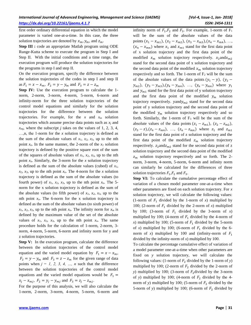
International Journal of Advanced Engineering, Management and Science (IJAEMS) [Vol-4, Issue-1, Jan- 2018]
https://dx.doi.org/10.22161/ijaems.4.1.7 ISSN: 2454-1311
www.ijaems.com Page | 31
first order ordinary differential equation in which the model
parameter is varied one-at-a-time. In this case, the three
solution trajectories are denoted by 𝑥𝑚, 𝑦𝑚, and 𝑧𝑚 .
Step III : code an appropriate Matlab program using ODE
Runge-Kutta scheme to execute the program in Step I and
Step II. With the initial conditions and a time range, the
execution program will produce the solution trajectories for
the programs in step I and step II.
On the execution program, specify the difference between
the solution trajectories of the codes in step I and step II
as 𝐹1 = 𝑥 − 𝑥𝑚, 𝐹2 = 𝑦 − 𝑦𝑚 and 𝐹3 = 𝑧 − 𝑧𝑚
Step IV: Use the execution program to calculate the 1-
norm, 2-norm, 3-norm, 4-norm, 5-norm, 6-norm and
infinity-norm for the three solution trajectories of the
control model equations and similarly for the solution
trajectories for the difference between the solution
trajectories. For example, for the x and xm solution
trajectories which assume precise data points such as xj and
xmj, where the subscript j takes on the values of 1, 2, 3, 4,
…,n, the 1-norm for the x solution trajectory is defined as
the sum of the absolute values of x1, x2, x3, up to the nth
point xn. In the same manner, the 2-norm of the x1 solution
trajectory is defined by the positive square root of the sum
of the squares of absolute values of x1, x2, x3, up to the nth
point xn. Similarly, the 3-norm for the x solution trajectory
is defined as the sum of the absolute values (cubed) of x1,
x2, x3, up to the nth point xn. The 4-norm for the x solution
trajectory is defined as the sum of the absolute values (to
fourth power) of x1, x2, x3, up to the nth point xn. The 5-
norm for the x solution trajectory is defined as the sum of
the absolute values (to fifth power) of x1, x2, x3, up to the
nth point xn. The 6-norm for the x solution trajectory is
defined as the sum of the absolute values (to sixth power) of
x1, x2, x3, up to the nth point xn. The infinity norm for xm is
defined by the maximum value of the set of the absolute
values of x1, x2, x3, up to the nth point xn. The same
procedure holds for the calculation of 1-norm, 2-norm, 3-
norm, 4-norm, 5-norm, 6-norm and infinity norm for y and
z solution trajectories.
Step V: In the execution program, calculate the difference
between the solution trajectories of the control model
equation and the varied model equation by 𝐹1 = 𝑥 − 𝑥𝑚,
𝐹2 = 𝑦 − 𝑦𝑚 and 𝐹3 = 𝑧 − 𝑧𝑚 for the given range of data
points when j = 1, 2, 3, 4, …, n such that the difference
between the solution trajectories of the control model
equations and the varied model equations would be 𝐹1 =
𝑥𝑗 − 𝑥𝑚𝑗, 𝐹2 = 𝑦𝑗 − 𝑦𝑚𝑗 and 𝐹3 = 𝑧𝑗 − 𝑧𝑚𝑗 .
For the purpose of this analysis, we will also calculate the
1-norm, 2-norm, 3-norm, 4-norm, 5-norm, 6-norm and
infinity norm of 𝐹1,𝐹2 and 𝐹3. For example, 1-norm of F1
will be the sum of the absolute values of the data
points (𝑥1 − 𝑥𝑚1), (𝑥2 − 𝑥𝑚2), (𝑥3 − 𝑥𝑚3),(𝑥4 − 𝑥𝑚4), …,
(𝑥𝑛 − 𝑥𝑚𝑛) where 𝑥1 and 𝑥𝑚1 stand for the first data point
of x solution trajectory and the first data point of the
modified 𝑥𝑚 solution trajectory respectively. 𝑥2and𝑥𝑚2
stand for the second data point of x solution trajectory and
the second data point of the modified 𝑥𝑚 solution trajectory
respectively and so forth. The 1-norm of F2 will be the sum
of the absolute values of the data points (𝑦1 − 𝑦), (𝑦2 −
𝑦𝑚2), (𝑦3 − 𝑦𝑚3),(𝑦4 − 𝑦𝑚4), …, (𝑦𝑛 − 𝑦𝑚𝑛) where 𝑦1
and 𝑦𝑚1 stand for the first data point of y solution trajectory
and the first data point of the modified 𝑦𝑚 solution
trajectory respectively. 𝑦and𝑦𝑚2 stand for the second data
point of y solution trajectory and the second data point of
the modified 𝑦𝑚 solution trajectory respectively and so
forth. Similarly, the 1-norm of F3 will be the sum of the
absolute values of the data points (𝑧1 − 𝑧𝑚1), (𝑧2 − 𝑧𝑚2),
(𝑧3 − 𝑧),(𝑧4 − 𝑧𝑚4), …, (𝑧𝑛 − 𝑧𝑚𝑛) where 𝑧1 and 𝑧𝑚1
stand for the first data point of z solution trajectory and the
first data point of the modified 𝑧𝑚 solution trajectory
respectively. 𝑧2and𝑧𝑚2 stand for the second data point of z
solution trajectory and the second data point of the modified
𝑧𝑚 solution trajectory respectively and so forth. The 2-
norm, 3-norm, 4-norm, 5-norm, 6-norm and infinity norm
can similarly be calculated for the differences of three
solution trajectories 𝐹1,𝐹2 and 𝐹3.
Step VI: To calculate the cumulative percentage effect of
variation of a chosen model parameter one-at-a-time when
other parameters are fixed on each solution trajectory. For x
solution trajectory, we will calculate the following values:
(1-norm of 𝐹1 divided by the 1-norm of x) multiplied by
100; (2-norm of 𝐹1 divided by the 2-norm of x) multiplied
by 100; (3-norm of 𝐹1 divided by the 3-norm of x)
multiplied by 100; (4-norm of 𝐹1 divided by the 4-norm of
x) multiplied by 100; (5-norm of 𝐹1 divided by the 5-norm
of x) multiplied by 100; (6-norm of 𝐹1 divided by the 6-
norm of x) multiplied by 100 and (infinity-norm of 𝐹1
divided by the infinity-norm of x) multiplied by 100.
To calculate the percentage cumulative effect of variation of
a model parameter one-at-a-time when other parameters are
fixed on y solution trajectory, we will calculate the
following values: (1-norm of 𝐹2 divided by the 1-norm of y)
multiplied by 100; (2-norm of 𝐹2 divided by the 2-norm of
y) multiplied by 100; (3-norm of 𝐹2divided by the 3-norm
of y) multiplied by 100; (4-norm of 𝐹2 divided by the 4-
norm of y) multiplied by 100; (5-norm of 𝐹2 divided by the
5-norm of y) multiplied by 100; (6-norm of 𝐹2 divided by

International Journal of Advanced Engineering, Management and Science (IJAEMS) [Vol-4, Issue-1, Jan- 2018]
https://dx.doi.org/10.22161/ijaems.4.1.7 ISSN: 2454-1311
www.ijaems.com Page | 32
the 6-norm of y) multiplied by 100 and (infinity-norm of 𝐹2
divided by the infinity-norm of y) multiplied by 100.
To calculate the percentage cumulative effect of variation of
a model parameter one-at-a-time when other parameters are
fixed on z solution trajectory, we will calculate the
following values: (1-norm of 𝐹3divided by the 1-norm of z)
multiplied by 100; (2-norm of 𝐹3 divided by the 2-norm of
z) multiplied by 100; (3-norm of 𝐹3 divided by the 3-norm
of z) multiplied by 100; (4-norm of 𝐹3 divided by the 4-
norm of z) multiplied by 100; (5-norm of 𝐹3 divided by the
5-norm of z) multiplied by 100; (6-norm of 𝐹3 divided by
the 6-norm of z) multiplied by 100 and (infinity-norm of 𝐹3
divided by the infinity-norm of z) multiplied by 100.
Due to the unstable values of the 1-norm, 2-norm, 3-norm,
4-norm, 5-norm, 6-norm and infinity-norm specifications,
we adopt to use a compact value for related percentage
values of these norms. For example, the cumulative
percentage value of 1-norm sensitivity in terms of the
difference in solution trajectories involves the sum of the 1-
norm values due to 𝐹1 solution trajectory, 1-norm values
due to 𝐹2 solution trajectory and 1-norm values due to 𝐹3
solution trajectory. The same procedure can be followed to
calculate the cumulative percentage values for 3-norm, 3-
norm, 4-norm, 5-norm, 6-norm and infinity-norm
sensitivities in terms of 𝐹1 solution trajectory, 𝐹2 solution
trajectory and 𝐹3 solution trajectory.
The cardinal points of sensitivity analysis results
interpretation are:
the parameter which when varied a little and
produces the biggest cumulative effect on the
solution trajectories is called a most sensitive
parameter. And it is highly uncertain. This by
implication will attract error in prediction and thus
require further validation.
the parameter which when varied a little
andproduces lower or least sensitivity values is
called a less or least sensitive parameter and
requires lesser validation.
Method for Best-fit parameter value selection
In order to select the best-fit parameter value for each
model parameter, we recommend that
At 100% variation, the coordinates of the solution
trajectories have same values, sums, squares and
square roots = 0. Therefore, the norm values at
100% are zero.
The Local minimum value is selected at a point where the
smallest norm value occurs before or after the 100%
variation.
IV. RESULTS AND DISCUSSION
On the application of the define method of analysis, we hereby present and discuss the following results:
Table.1: sensitivity analysis results for model parameter r
r 1-norm 2-norm 3-norm 4-norm 5-norm 6-norm ∞-norm
0.0030 143.9520 78.8284 82.0093 66.2747 56.624 50.6594 29.8099
0.0060 143.1933 78.4409 81.6042 65.9501 56.348 50.4130 29.6754
0.0090 142.3997 78.0321 81.1766 65.6070 56.056 50.1521 29.5334
0.0120 141.5698 77.6010 80.7256 65.2447 55.747 49.8763 29.3837
0.0150 140.7023 77.1468 80.2503 64.8624 55.421 49.5850 29.2259
0.0180 139.7958 76.6685 79.7499 64.4593 55.077 49.2776 29.0605
0.0210 138.8491 76.1654 79.2236 64.0350 54.715 48.9538 28.8879
0.0240 137.8610 75.6368 78.6706 63.5887 54.334 48.6131 28.7078
0.0270 136.8304 75.0818 78.0903 63.1201 53.934 48.2553 28.5200
0.0300 135.7565 74.4999 77.4821 62.6287 53.514 47.8800 28.3243
What do we learn from Table 1?
We have observed from table 1 that as the value of the
model parameter r increases monotonically from 0.003
(approx) to 0.03 (approx), the 1-norm error data decreases
monotonically from the value of 143.95 (approx.) to 135.76
(approx.), the 2-norm error data decreases monotonically
from the value of 78.83 (approx.) to 75.50 (approx.), the 3-
norm error data decreases monotonically from the value of
82.01 (approx.) to 77.48 (approx.), the 4-norm error data
decreases monotonically from the value of 66.27 (approx.)
to 62.63 (approx.), the 5-norm error data decreases
monotonically from the value of 56.62 (approx.) to 53.51
(approx.), the 6-norm error data decreases monotonically
from the value of 50.66 (approx.) to 47.88(approx.) and the
infinity-norm error data decreases monotonically from the
value of 29.81 (approx.) to 28.32 (approx.).

International Journal of Advanced Engineering, Management and Science (IJAEMS) [Vol-4, Issue-1, Jan- 2018]
https://dx.doi.org/10.22161/ijaems.4.1.7 ISSN: 2454-1311
www.ijaems.com Page | 33
On the basis of this present analysis we have observed that r
= 0.003 is associated with relatively higher uncertainty
when compared to the value of r = 0.03 irrespective of the
type of p-norm we have used to calculate the sensitivity
analysis. Despite the observed uncertainty analysis results
due to a one percent to ten percent variation of the intrinsic
growth rate of the fish population, it is clear that the
statistical range of the p-norm sensitivity values are listed as
follows: the range of 1-norm statistical range is 8.19, the
range of 2-norm statistical range is 3.33,the range of 3-norm
statistical range is 4.53,the range of 4-norm statistical range
is 3.64,the range of 5-norm statistical range is 3.11,the
range of 6-norm statistical range is 2.78 ,the range of
infinity-norm statistical range is 1.49.
These bigger sensitivity values which indicate high
uncertainty of the intrinsic growth rate of the fish
population can be further minimized.
Table.2: local minimum resultsfor parameter r
r 1-norm 2-norm 3-norm 4-norm 5-norm 6-norm ∞-norm
0.2880 4.3024 2.2917 2.4375 2.0011 1.739 1.5812 1.0897
0.2910 3.2128 1.7106 1.8194 1.4936 1.298 1.1803 0.8137
0.2940 2.1326 1.1350 1.2072 0.9910 0.861 0.7831 0.5401
0.2970 1.0617 0.5648 0.6007 0.4931 0.429 0.3897 0.2688
0.3000 0.0000 0.0000 0.0000 0.0000 0.000 0.0000 0.0000
0.3030 1.0527 0.5595 0.5951 0.4885 0.425 0.3860 0.2663
0.3060 2.0964 1.1138 1.1847 0.9724 0.845 0.7685 0.5304
0.3090 3.1314 1.6630 1.7688 1.4517 1.262 1.1473 0.7926
0.3120 4.1577 2.2071 2.3475 1.9265 1.674 1.5225 1.0527
0.3150 5.1755 2.7463 2.9209 2.3969 2.083 1.8943 1.3106
What do we learn from Table 2?
Table 2 shows a result of the cumulative effect of 96 to 105
percent variation of model parameter r. At 100percent
variation, there are no changes in the original and the varied
solution trajectories, hence the zero values.
Observe that as the model parameter value increase
monotonically from a low value of 0.2880 to 0.0000
corresponding to 100 percent variation and then increases
monotonically to 0.3150 approximately in column I, the 1-
norm sensitivity value decreased monotonically from a
value of 4.30 to 0.0000 corresponding 100 percent variation
and then increases monotonically to 5.18 approximately in
column II, the 2- norm sensitivity value decreased
monotonically from a value of 2.29 to 0.0000 corresponding
100percent variation and then increases monotonically to
2.75 approximately in column III, the 3- norm sensitivity
value decreased monotonically from a value of 2.44 to
0.0000 corresponding 100percent variation and then
increases monotonically to 2.92 approximately in column
IV, the 4- norm sensitivity value decreased monotonically
from a value of 2.00 to 0.0000 corresponding 100percent
variation and then increases monotonically to 2.40
approximately in column V, the 5- norm sensitivity value
decreased monotonically from a value of 1.74 to 0.0000
corresponding 100percent variation and then increases
monotonically to 2.08 approximately in column VI, the 6-
norm sensitivity value decreased monotonically from a
value of 1.58 to 0.0000 corresponding 100percent variation
and then increases monotonically to 1.90 approximately in
column VII, the infinity- norm sensitivity value decreased
monotonically from a value of 1.09 to 0.0000 corresponding
100percent variation and then increases monotonically to
1.31 approximately in column VIII.
The local minimum is selected at the greatest lower bound
of the data points for each p-norm results. For instance, the
local minimum value for model parameter r is 0.303 where
1-norm local minimum value = 1.0527, 2-norm local
minimum value = 0.5595, 3-norm local minimum value =
0.0.5951, 4-norm local minimum value = 0.4885, 5-norm
local minimum value = 0.4250, 6-norm local minimum
value = 0.3860 and infinity-norm local minimum value =
0.2663.
V. CONCLUSION
This present study has been able to reduce the uncertainty in
the intrinsic growth rate of a fish population due to its
variations using a combination of a numerical scheme and
the mathematical p-norms. The present results compliment
the earlier contribution of Ekaka-a et al (2012) that only
considered the sensitivity analysis in the context of a shorter
experimental time. This present proposed numerical scheme
can be extended to study the sensitivity analysis of other

International Journal of Advanced Engineering, Management and Science (IJAEMS) [Vol-4, Issue-1, Jan- 2018]
https://dx.doi.org/10.22161/ijaems.4.1.7 ISSN: 2454-1311
www.ijaems.com Page | 34
model parameter values which we did not consider in this
study in our future investigation.
REFERENCES
[1] E. N. Ekaka-a, N. M. Nafo, A. I. Agwu, (2012),
Examination of extent of sensitivity of a mathematical
model parameter of survival of species dependent on a
resource in a polluted environment, International
Journal of Information Science and Computer
Mathematics, vol. 8, no 1-2, pp 1-8.
[2] EnuEkaka-a, Olowu, B. U., Eze F. B., Abubakar R. B.,
Agwu I. A., Nwachukwu E. C., (2013), Journal of
Nigerian Association of Mathematical Physics, Vol
23, pp 177-182.
[3] Palumbi S. (1999). The ecology of marine protected
areas: Working paper from the Department of
Organismic and Evolutionary Biology, Harvard
University.
[4] Rodwell L. D, Edward B. Barbier, Callum M. Roberts,
Tim R. Mcclanahan (2002), A model of tropical
marine reserve-fishery linkages. Natural Resource
Modeling, 15(4).
[5] Sumalia U. (2002) Marine protected area performance
in a model of the fishery. Natural Resource Modeling,
15(4).
[6] J. Pitchford, E.Codling, D. Psarra. Uncertainty and
sustainability in fisheries.Ecological Modelling, 2007,
207: 286–292.
[7] Kar, T. and Chakraborty, K. (2009): Marine reserves
and its consequences as a fisheries management tool,
World Journal of Modelling and Simulation, (2009)
5(2), pp. 83-95.
[8] J. Bohnsack. Marine reserves: They enhance fisheries,
reduce conflicts, and protect resources. Oceanus,
1993,63–71.
[9] Hamby, D.M. (1994). A review of techniques for
parameter sensitivity analysis of environmental
models, Environmental Monitoring and
Assessment 32: 135-154.

International Journal of Advanced Engineering, Management and Science (IJAEMS) [Vol-4, Issue-1, Jan- 2018] 1311-ISSN: 2454 x.doi.org/10.22161/ijaems.4.1.8https://d
35| Page www.ijaems.com
Rates of Soft Ground Tunneling in Vicinity of
Existing Structures Ayman S. Shehata1, Adel M. El-Kelesh2, Al-Sayed E. El-kasaby1, Mustafa Mansour1
1Department of Civil Engineering, Benha Faculty of Engineering, Benha University, Egypt
2Construction Engineering and Utilities Department, Faculty of Engineering, and Geo-Construction Research and
Development Center (GRDC-ZU), Zagazig University, Egypt
Abstract— Soft ground tunneling in the vicinity of
existing structures is a major challenge to tunneling
engineers. Tunneling works cause inevitable ground
movements that may lead to unrecoverable damages to
adjacent structures. Tunneling rates significantly affect
such risks. However, a guideline that determines
appropriate tunneling rates and accounts for the effects of
tunneling on the structures existing in the vicinity is not
available. Tunneling records in terms of TBM advance
speed (AS), utilization factor (U), and advance rate (AR)
for tunnels constructed without causing significant risks
on the existing structures are presented in the
paper.These records are discussed for different types of
existing structures.Ranges of these records for tunneling
without causing detrimental effects on different types
existing structures are recommended.Useful observations
are also made on the variation of these records with the
ground type and composition and the precautions to be
adopted to mitigate the tunneling risks on existing
structures.
Keywords— Soft ground, mechanized tunneling,
utilization factor, ground conditions, tunnel boring
machine (TBM), productivity, advance speed, advance
rate.
I. INTRODUCTION
The term ‘Hard Point’ is used to describe the structures
that exist in the vicinity oftunneling works. The hard
points includefor instance buildings, footings of bridges
and underground utilities such asshafts, sewer tunnels and
electrical cables. Excavation by tunnel boring machines
(TBMs) inevitably results in ground movements that may
cause adjacent structures to deform, distort, and possibly
sustain unrecoverable damages. A determination of the
appropriate tunneling method that mitigates the tunneling
risks on adjacent structures is a major challenge in soft
ground tunneling. The difficulty stems from the many and
critical factors involved in the process, such as the
potential for ground loss because of tunneling, variable
ground conditions under a hard point, and effect of
tunneling on the integrity of existing structures.
Tunneling advance rate, as a tunneling parameter, has
been reported as a factor that affects the ground
movements caused by TBM excavation (e.g., Toan and
Hung 2007).
Tunnel construction duration is a critical factor in
tunneling projects and is estimated on the basis of the
tunneling advance rate as follows:
𝐷 =𝐿
𝐴𝑅 (1)
where D (days) = construction duration, L (m) = length of
tunnel, and AR (m/day) = advance rate of TBM and is
defined as the distance of boring and ring erection divided
by the total time (shift or day). AR is determined using the
following expression
𝐴𝑅 =𝐴𝑆 × 𝑈 × 60 × 24
100000 (2)
where AS (mm/min) = advance speed of TBM and is
defined as the stroke length of TBM into the ground
divided by the operating time of excavation (i.e. the
instantaneous penetration rate of TBM), and U (%) =
utilization factor of TBM and is defined as the time of
excavation by TBM divided by the total time. Therefore,
accurate determination of AR or AS and U is necessary for
the development of reliable tunnel construction time plans
and cost estimate and control.
Management of tunneling works in the vicinity of hard
points and the relevant risks necessitates determination of
appropriate AR at the hard points. A guideline that
determines AR in soft ground in the vicinity of hard points
is not available.AR is usually determined on the basis of
empiricism and experiences of practitioners. Little effort
however has been made to establish a guideline that
determines AR and accounts for the different types and
conditions of hard points. Moreover, the literature lacks
reported data on ARand the corresponding effects on hard
points. The current paper presents field records of AR, AS,
and U for tunnels actually constructed in Egypt in the
vicinity of existing hard points. It also discusses these
records for different types of hard points. The paper starts
with an elaboration of the effects of tunneling works and
rates on the conditions of existing structures in the
vicinity of tunneling works. This is followed by a brief
description of the project from which the records were
obtained. Then, the records are presented and discussed.

International Journal of Advanced Engineering, Management and Science (IJAEMS) [Vol-4, Issue-1, Jan- 2018] 1311-ISSN: 2454 x.doi.org/10.22161/ijaems.4.1.8https://d
36| Page www.ijaems.com
II. EFFECT OF TUNNELING RATES ON
CONDITION OF EXISTING STRUCTURES
Volumes of excavation larger than the volume of ground
occupied by a tunnel are not uncommon in tunneling.
Such differences in volumes, known as volume losses,
inevitably result in ground movements. Toan and Hung
(2007) reported that the net volume of surface settlement
trough in most ground conditions is approximately equal
to the volume loss because of tunneling. Such ground
movements may cause adjacent structures to deform,
rotate, distort, and possibly sustain unrecoverable
damages (Zhang et al. 2012). Toan and Hung (2007) also
indicated that the magnitude of volume loss depends on
many different factors such as the tunneling method,
tunneling advance rate, tunnel size, and ground type. The
existence of structures in the vicinity of a constructed
tunnel is therefore rated among the highrisk factors in
tunneling in urban areas (Kovari 2004).
It has been reported that the tunneling induced ground
movements and thus the risks on adjacent structures can
be mitigated by adopting the following measures (e.g.,
Toan and Hung 2007; Goh et al. 2016; Sheng et al. 2016):
- Adopting appropriate tunneling advance rates to
minimize the ground movements caused by the
machine ground interaction.
- Adopting larger thrust forces to increase the
depth of cutting and maintain the desired
advance speed.
- Monitoring the lateral movement of tunnels to
ensure that the generated drag forces have
insignificant impact on the existing structures.
- The minimum pressure applied at the face should
be slightly higher than the hydrostatic pressure,
particularly when going below existing
structures. This is done mainly by controlling the
rotational speed of the screw and the amount of
muck discharge at the outlet of the screw
conveyor.
- Setting the cutterhead rotation to low revolutions
so that any torque spikes that are indicative of
obstructions encountered during the course of
crossing sensitive structures are easily detected.
- Erecting the lining immediately after excavation
and providing tight control of the tunneling
process.
- Pre-planning for cutterhead interventions just
before the TBMs go below existing structures for
checking the cutterhead condition and making
any necessary replacements of the cutting tools.
Sheng et al. 2016 reported a significant case history on
the tunneling of the Downtown Line Stage 3 (DTL3) of
Mass Rapid Transit (MRT) system across Singapore
Island. The DTL3 alignment is overcrossing the existing
North East Line (NEL) rail tunnel and undercrossing the
existing North South Line (NSL) and Circle Line (CCL)
with clear distance of less than one bored tunnel diameter,
and overburden ranges from 20.0 to 45.0 m; the diameter
of DTL3 is 6.35 m. DTL3 is located approximately 1.3 m
above NEL tunnel, 8.7 m below NSL tunnel and 3.3 m
below CCL tunnel. The ground consists mainly of
siltstone with layers of mudstones and sandstone. They
observed that the advance speed of the TBM was reduced
to less than 5, 10 – 13, and 8 – 15 mm/min when
overcrossing NEL, undercrossing NSL, and
undercrossing CCL, respectively.
The aforementioned reveals that TBM tunneling in soft
ground may cause significantly detrimental effects on
existing structures in the vicinity. In addition, tunneling
rate is an important factor that significantly affects the
conditions of existing structures in the vicinity of
tunneling. Therefore, appropriate tunneling rates should
be determined to mitigate tunneling risks on adjacent
structures.
III. PROJECT DESCRIPTION AND GROUND
CONDITIONS
The network of the Greater Cairo metro consists of three
lines (Lines 1 to 3) as shown in Fig. 1. Line 3 is
approximately 47.87 km long and consists of 39 stations.
The construction of the line has been divided into four
main phases as indicated in Figs. 1 and 2 and summarized
in Table 1. At the time of publishing this paper, the
construction of Phases 1 and 2 has been completed, Phase
3 has been under study, and Phase 4 has
beingconstructed. The types of TBMs used in the line are
indicated in Fig. 2 and Table 1. Phases 1and 4A were
fully excavated using slurry TBMs (TBM 1 and 2 for
Phase1 and TBM 4 for Phase 4A) and constructed in 24
and 14 months, respectively. However, Phase 2 was fully
excavated in 26 months using two different types of
TBMs: Slurry and EPB TBMs.The tunnel segment
extending from Abbasia station to Cairo Fair station (Lot
11-c) was fully excavated using TBM 2, while that
extending from Cairo Fair station to Haroun station was
fully excavated using EPB TBM (TBM 3).
Field records of the construction of Lot 11-c (Phase 2A),
approximately 1,950 m in length, are used in the current
paper. The records indicate that the construction of this
phase progressed at a rate of 11.0 m per working day. A
photo of the used TBM (TBM2) is shown in Fig. 3 and its
general specifications are summarized in Table 2.In the
construction of Lot 11-c, TBM 2 was excavating under
many hard points which include different types of
existing structure such as buildings, footings of Bridges,
sewer tunnels, annexed structure and tunnel shafts. A
general description of the hard points at the location of
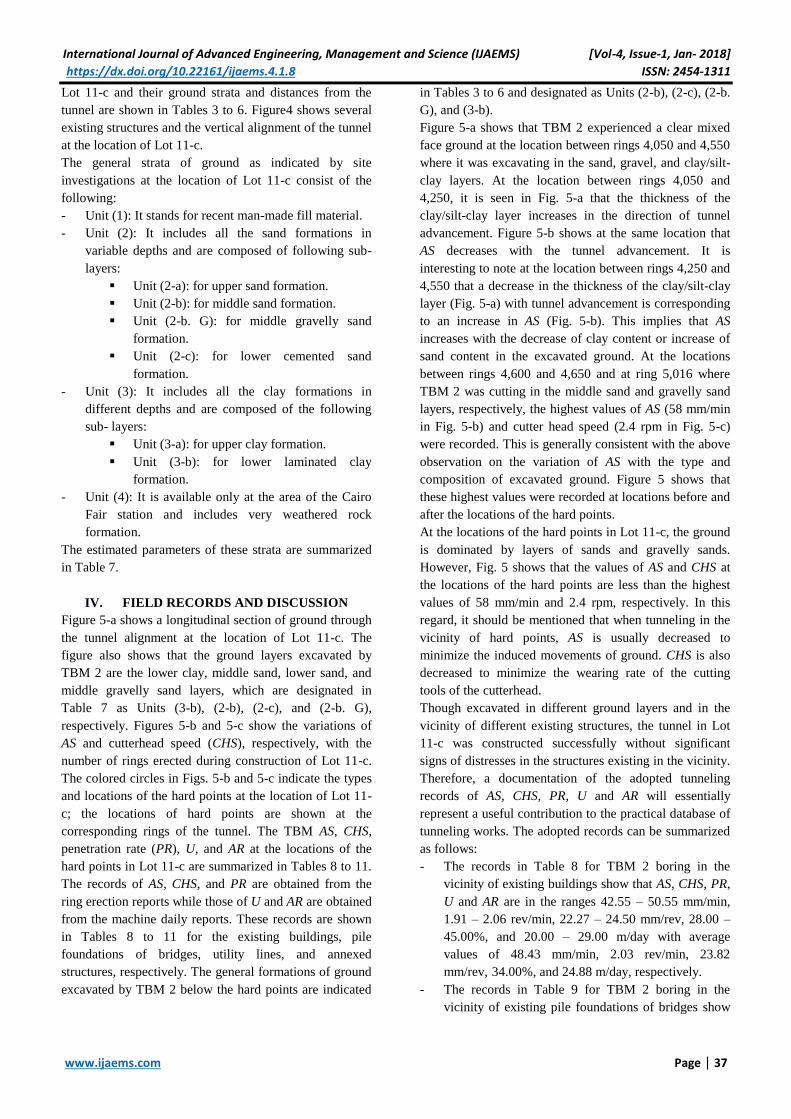
International Journal of Advanced Engineering, Management and Science (IJAEMS) [Vol-4, Issue-1, Jan- 2018] 1311-ISSN: 2454 x.doi.org/10.22161/ijaems.4.1.8https://d
37| Page www.ijaems.com
Lot 11-c and their ground strata and distances from the
tunnel are shown in Tables 3 to 6. Figure4 shows several
existing structures and the vertical alignment of the tunnel
at the location of Lot 11-c.
The general strata of ground as indicated by site
investigations at the location of Lot 11-c consist of the
following:
- Unit (1): It stands for recent man-made fill material.
- Unit (2): It includes all the sand formations in
variable depths and are composed of following sub-
layers:
Unit (2-a): for upper sand formation.
Unit (2-b): for middle sand formation.
Unit (2-b. G): for middle gravelly sand
formation.
Unit (2-c): for lower cemented sand
formation.
- Unit (3): It includes all the clay formations in
different depths and are composed of the following
sub- layers:
Unit (3-a): for upper clay formation.
Unit (3-b): for lower laminated clay
formation.
- Unit (4): It is available only at the area of the Cairo
Fair station and includes very weathered rock
formation.
The estimated parameters of these strata are summarized
in Table 7.
IV. FIELD RECORDS AND DISCUSSION
Figure 5-a shows a longitudinal section of ground through
the tunnel alignment at the location of Lot 11-c. The
figure also shows that the ground layers excavated by
TBM 2 are the lower clay, middle sand, lower sand, and
middle gravelly sand layers, which are designated in
Table 7 as Units (3-b), (2-b), (2-c), and (2-b. G),
respectively. Figures 5-b and 5-c show the variations of
AS and cutterhead speed (CHS), respectively, with the
number of rings erected during construction of Lot 11-c.
The colored circles in Figs. 5-b and 5-c indicate the types
and locations of the hard points at the location of Lot 11-
c; the locations of hard points are shown at the
corresponding rings of the tunnel. The TBM AS, CHS,
penetration rate (PR), U, and AR at the locations of the
hard points in Lot 11-c are summarized in Tables 8 to 11.
The records of AS, CHS, and PR are obtained from the
ring erection reports while those of U and AR are obtained
from the machine daily reports. These records are shown
in Tables 8 to 11 for the existing buildings, pile
foundations of bridges, utility lines, and annexed
structures, respectively. The general formations of ground
excavated by TBM 2 below the hard points are indicated
in Tables 3 to 6 and designated as Units (2-b), (2-c), (2-b.
G), and (3-b).
Figure 5-a shows that TBM 2 experienced a clear mixed
face ground at the location between rings 4,050 and 4,550
where it was excavating in the sand, gravel, and clay/silt-
clay layers. At the location between rings 4,050 and
4,250, it is seen in Fig. 5-a that the thickness of the
clay/silt-clay layer increases in the direction of tunnel
advancement. Figure 5-b shows at the same location that
AS decreases with the tunnel advancement. It is
interesting to note at the location between rings 4,250 and
4,550 that a decrease in the thickness of the clay/silt-clay
layer (Fig. 5-a) with tunnel advancement is corresponding
to an increase in AS (Fig. 5-b). This implies that AS
increases with the decrease of clay content or increase of
sand content in the excavated ground. At the locations
between rings 4,600 and 4,650 and at ring 5,016 where
TBM 2 was cutting in the middle sand and gravelly sand
layers, respectively, the highest values of AS (58 mm/min
in Fig. 5-b) and cutter head speed (2.4 rpm in Fig. 5-c)
were recorded. This is generally consistent with the above
observation on the variation of AS with the type and
composition of excavated ground. Figure 5 shows that
these highest values were recorded at locations before and
after the locations of the hard points.
At the locations of the hard points in Lot 11-c, the ground
is dominated by layers of sands and gravelly sands.
However, Fig. 5 shows that the values of AS and CHS at
the locations of the hard points are less than the highest
values of 58 mm/min and 2.4 rpm, respectively. In this
regard, it should be mentioned that when tunneling in the
vicinity of hard points, AS is usually decreased to
minimize the induced movements of ground. CHS is also
decreased to minimize the wearing rate of the cutting
tools of the cutterhead.
Though excavated in different ground layers and in the
vicinity of different existing structures, the tunnel in Lot
11-c was constructed successfully without significant
signs of distresses in the structures existing in the vicinity.
Therefore, a documentation of the adopted tunneling
records of AS, CHS, PR, U and AR will essentially
represent a useful contribution to the practical database of
tunneling works. The adopted records can be summarized
as follows:
- The records in Table 8 for TBM 2 boring in the
vicinity of existing buildings show that AS, CHS, PR,
U and AR are in the ranges 42.55 – 50.55 mm/min,
1.91 – 2.06 rev/min, 22.27 – 24.50 mm/rev, 28.00 –
45.00%, and 20.00 – 29.00 m/day with average
values of 48.43 mm/min, 2.03 rev/min, 23.82
mm/rev, 34.00%, and 24.88 m/day, respectively.
- The records in Table 9 for TBM 2 boring in the
vicinity of existing pile foundations of bridges show

International Journal of Advanced Engineering, Management and Science (IJAEMS) [Vol-4, Issue-1, Jan- 2018] 1311-ISSN: 2454 x.doi.org/10.22161/ijaems.4.1.8https://d
38| Page www.ijaems.com
that AS, CHS, PR, U and AR are in the ranges 29.44 –
48.09 mm/min, 1.72 – 1.89 rev/min, 17.19 – 25.39
mm/rev, 33.00 – 42.00%, and 21.00 – 22.00 m/day
with average values of 38.76 mm/min, 1.81 rev/min,
21.29 mm/rev, 38.00%, and 21.50 m/day,
respectively. At the location between rings 5,180 and
5,295 TBM 2 was boring between two groups of the
pile foundations of the existing 6th October Bridge
western ramp and under sewer tunnels. The distance
between the tunnel and one of the pile groups is
approximately 1.68 m (see Fig. 6). This is the
smallest distance between the tunnel and the hard
points throughout the tunnel alignment. At this
location, AS and CHS were significantly decreased to
29.44 mm/min and 1.72 rpm, respectively, and the
corresponding U was 42.00%.
- The records in Table 10 for TBM 2 boring under
existing utility tunnels of 1.00 – 2.25 m in diameter
show that AS, CHS, PR, U and AR are in the ranges
30.26 – 40.32 mm/min, 1.69 – 1.93 rev/min, 16.96 –
20.86 mm/rev, 42.00 – 43.00%, and 21.00 – 23.00
m/day with average values of 34.29 mm/min, 1.77
rev/min, 19.31 mm/rev, 34.00%, and 22.50 m/day,
respectively.
- The records in Table 11 for TBM 2 boring in
diaphragm walls of existing annexed structures show
that AS, CHS, PR, U and AR are in the ranges 9.80 –
12.70 mm/min, 2.03 – 2.31 rev/min, 5.00 – 6.00
mm/rev, 28.00 – 46.00%, and 5.00 – 6.00 m/day with
average values of 11.25 mm/min, 2.17 rev/min, 5.50
mm/rev, 37.00%, and 5.50 m/day, respectively (see
Fig. 7).
Figure 8 shows a representation of the average tunneling
records of AS, CHS and U for the types of hard points
existing in Lot 11-c.
It is worth mentioning that the relatively high values of U
recorded during tunneling in the vicinity of the hard
points in Lot 11-c are attributed to the following
additional precautionary measures:
1. The rings were erected immediately after
excavation. This contributed to the reduction
of the delay times.
2. Hyperbaric interventions were routinely
made before starting excavation in the
vicinity of the hard points. This increases
the cutting efficiency of the cutterhead in
the ground and mitigates any residual risks.
3. Larger thrust forces were applied to increase
the depth of cutting of the cutter tools and to
maintain the advance speed.
A reduction in the delay and maintenance times
contributes to the increase of U.
V. SUMMARY AND CONCLUSIONS
TBM tunneling in soft grounds inevitably results in
ground movements that may cause unrecoverable
damages to adjacent structures. The effects of TBM
tunneling on adjacent structures are briefly reviewed in
the paper. Management of tunneling works in the vicinity
of existing structures (hard points) and the relevant risks
necessitates determination of appropriate tunneling rates
at the hard points. A guideline that determines appropriate
rates of tunneling in the vicinity of hard points is not
available. Moreover, the literature lacks reported data on
tunneling rates and the corresponding effects on hard
points. As a contribution to the database of tunneling
works, the current paper presents field records of TBM
tunneling advance speed (AS), utilization factor (U), and
advance rate (AR) that are obtained from tunnels actually
constructed in Egypt in the vicinity of hard points. It also
discusses these records for different types of hard points:
buildings, pile foundations, utility tunnels, and annexed
structures. Ranges of AS, U, and AR for TBM tunneling
without significant risks on the structures existing in the
vicinity of tunneling works are also presented. In
addition, observations and discussions on the variation of
AS, U, and AR with the ground type and composition and
precautions to be adopted to mitigate risks of tunneling on
structures in the vicinity are presented in the paper.
REFERENCES
[1] Arshad, and Abdullah, R.A. (2016). "A review on
selection of tunneling method and parameters
affecting ground settlements," Electronic Journal of
Geotechnical Engineering, Vol. 21, 4459–4475.
[2] Goh, K.H., Ng, S.S.G., and Wong, K.C. (2016).
"Case histories of bored tunneling below buildings in
Singapore downtown line," International Journal of
Geoengineering Case histories, Vol. 3, 149–161.
[3] ITA (International Tunneling Assocation) (2000).
"Mechanized tunneling, recommendations and
guidelines for tunnel boring machines
(TBMs),"Working Group 14, 1 – 118.
[4] Kovari, K., and Ramoni, M. (2004)." Key note
lecture at international congress on mechanized
tunneling: challenging case histories," Urban
tunneling in soft ground using TBM's, Politecnico di
Torino, Italy, 16–19.
[5] Multi-Mode TBM. (2017). "TBM information,"
<https://www.herrenknecht.com/en/innovation/resear
ch-development/machinescomponents/multi-mode-
tbm.html>(Aug. 20, 2017).
[6] NAT (National Authority for Tunnels)
(2017)."Information of greater Cairo metro line-3,"
Line-3, <http://www.nat.org.eg/english/Line3.html>
(Aug. 20, 2017).

International Journal of Advanced Engineering, Management and Science (IJAEMS) [Vol-4, Issue-1, Jan- 2018] 1311-ISSN: 2454 x.doi.org/10.22161/ijaems.4.1.8https://d
39| Page www.ijaems.com
[7] Ozfirat, M.K. (2015). "Selection of tunneling
machines in soft ground by fuzzy analytic hierarchy
process," DokuzEylul University, Acta
MontanisticaSlovaca, Vol. 20, No. 2, 98–109.
[8] Sheng, E. S. Y., Chuan, J. Y. T., Ikhyung, H. K.,
Osborne, N. H., Boon, C. K., and Siew, R. (2016). "
Tunneling undercrossing existing live MRT tunnels,"
Tunneling and Underground Space Technology, Vol.
57, 241–256.
[9] Shield Tunneling (2017). <http://helpiks.org/2-
30162.html> (Aug. 20, 2017).
[10] Thomas, W.P. (2011)."Tunneling beneath open
water, a practical guide for risk management and site
investigations," Professional Associate Finalist,
William Barclay Parsons Fellowship Program,
Parsons Brinckerhoff, New York.
[11] Toan, D. N., Hung, L. X. (2007)."Some aspects of
risk management and subsidence," Hanoi Metro Pilot
Line Project, Report at the Meeting between ITA and
ITST on Tunneling, Hanoi.
[12] Zhang, D., Fang, Q., Hou, Y. Li, P., and Yuen, W. L.
(2012)."Protection of buildings against damages as a
result of adjacent large-span tunneling in shallowly
buried soft ground," Journal of Geotechnical and
Geo-Environmental Engineering, Vol. 139, 903–13.
Fig. 1: Network of the Greater Cairo metro and route of Line 3 (NAT 2017).
Fig. 2: Construction phases of Line 3 and the used TBMs.

International Journal of Advanced Engineering, Management and Science (IJAEMS) [Vol-4, Issue-1, Jan- 2018] 1311-ISSN: 2454 x.doi.org/10.22161/ijaems.4.1.8https://d
40| Page www.ijaems.com
Fig. 3: The slurry TBM used in Line 3, Lot 11-c (Phase 2A), of the Greater Cairo metro (NAT 2017).
Fig. 4: Tunnel alignment under existing structures at location of Lot 11-c (Phase 2A); TBMs are shown for illustration.

International Journal of Advanced Engineering, Management and Science (IJAEMS) [Vol-4, Issue-1, Jan- 2018] 1311-ISSN: 2454 x.doi.org/10.22161/ijaems.4.1.8https://d
41| Page www.ijaems.com
Fig. 5: Ground profile and TBM records at the location of Lot 11-c: (a) ground profile; (b) AS; (c) CH
Fig. 6: TBM 2 boring between pile foundations of 6th October bridge western ramp, Lot 11-c.

International Journal of Advanced Engineering, Management and Science (IJAEMS) [Vol-4, Issue-1, Jan- 2018] 1311-ISSN: 2454 x.doi.org/10.22161/ijaems.4.1.8https://d
42| Page www.ijaems.com
Fig.7: TBM 2 crossing annexed structure 11-B, Lot 11-c: (a) vertical section; (b) plan view.
Fig.8: Average production records of TBM 2 for different types of hard points in the vicinity of tunneling works: (a) AS; (b)
CHS; (c) U.
0.00
10.00
20.00
30.00
40.00
50.00
60.00
Buildings PileFoundations
Sewer Tunnels Annexedstructure
TB
M a
dva
nce s
peed
, AS
(mm
/m
in)
Hard Points
0%
10%
20%
30%
40%
50%
60%
70%
Buildings PileFoundations
Sewer Tunnels Annexedstructure
TB
M u
tilizati
on, U
(%)
Hard Points
0.00
0.50
1.00
1.50
2.00
2.50
3.00
Buildings PileFoundations
Sewer Tunnels Annexedstructure
C.H
. speed
, CHS
(rpm
)
Hard Points
( a )
( c )
( b )

International Journal of Advanced Engineering, Management and Science (IJAEMS) [Vol-4, Issue-1, Jan- 2018] 1311-ISSN: 2454 x.doi.org/10.22161/ijaems.4.1.8https://d
43| Page www.ijaems.com
Table.1: Construction phases and types of TBMs used in Line 3 of the Greater Cairo metro.
Phase
#
Stage
# Tunnel Path
Stage Length
(km) TBM Type TBM No.
1 - From Attaba station to Abbasia station 4.3 Slurry TBM TBMs 1 & 2
2 A From Abbasia station to Cairo Fair station 1.95 Slurry TBM TBM 2
B From Cairo Fair station to Haroun station 5.75 EPBM TBM 3
3
A From Attaba station to Kit Kat station 4.00 --- Under study
B From Kit Kat station to Rod EL-Farag station 6.60 --- Under study
C From Kit Kat station to Cairo University station 7.20 --- Under study
4
A From Haroun station to El-Shams Club station 5.15 Slurry TBM 4
B From El-Shams Clubstation to Adly Mansour station 6.37 ----- Surface path
C From Helipolis station to Cairo Airport station 6.65 --- Under study
Table.2: General specifications of slurry TBM (TBM 2) used in Lot 11-c (Phase 2A) of Line 3.
Specification TBM 2
Shield diameter (m) 9.46
Shield length (m) 11.3
Max. advance speed (mm/min) 80
Max. rotational speed (rpm) 3
Max. thrust force (ton) 5500
Stroke length (m) 2
Max. torque of cutter head (ton.m) 2000
Cutting tools type: disc cutter, rippers, scrapers (no.) 22, 8, 168
Table.3: Existing buildings and their ground strata and distances from the tunnel at the location of Lot 11-c.
Building No. of Floors Ground Formation Vertical Distance to
Tunnel Crown (m)
Horizontal Distance
to Tunnel Axis (m)
11-c-31 1 Middle sandand clay 11.01 9.25
Oxygen Station 1 Middle sand 11.15 0
11-c-25 2 Middle sand 9.44 0
11-c-26 4 Middle sand 9.44 11
11-c-27 4 Middle sand 9.44 0
Ain Shams Hospital 1 Middle sand
andgravelly sand 9.45 0
Faculty of Arts 7 Gravelly sand 12.6 0
Ain Shams Information
Center-11-c-06 3
Gravelly sand
andmiddle sand 8.61 8.35
Table.4: Existing pile foundations of bridges and their ground strata and distances from the tunnel at the location of Lot 11-
c.
Pile Foundation Status Ground
Formation
Vertical Distance
to Tunnel Crown
(m)
Horizontal Distance
to Tunnel Axis (m)
Foundation of 6th
October Bridge Western
Ramp
Crossing between two
groups of pile foundations
Middle sand and
gravelly Sand 8.50 6.18
Foundation of 6th
October Bridge Eastern
Ramp
Crossing between two
groups of pile foundations
Middle sand
andgravelly sand 8.70 7.00
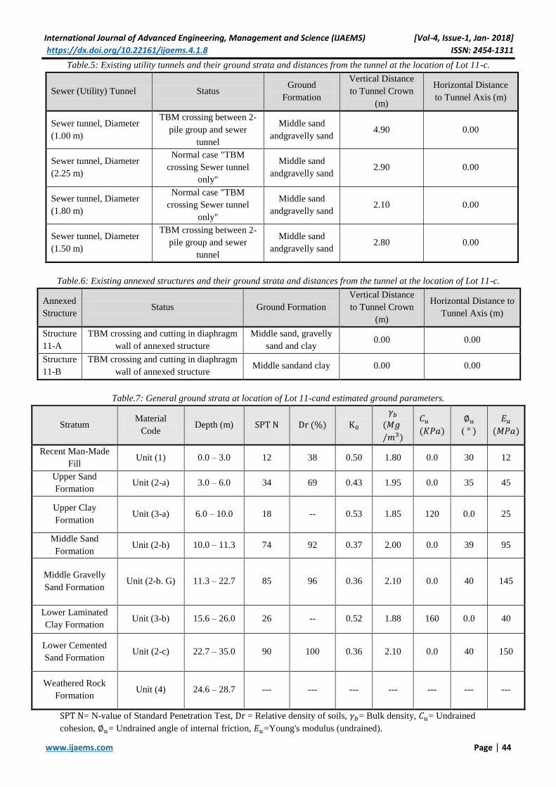
International Journal of Advanced Engineering, Management and Science (IJAEMS) [Vol-4, Issue-1, Jan- 2018] 1311-ISSN: 2454 x.doi.org/10.22161/ijaems.4.1.8https://d
44| Page www.ijaems.com
Table.5: Existing utility tunnels and their ground strata and distances from the tunnel at the location of Lot 11-c.
Sewer (Utility) Tunnel Status Ground
Formation
Vertical Distance
to Tunnel Crown
(m)
Horizontal Distance
to Tunnel Axis (m)
Sewer tunnel, Diameter
(1.00 m)
TBM crossing between 2-
pile group and sewer
tunnel
Middle sand
andgravelly sand 4.90 0.00
Sewer tunnel, Diameter
(2.25 m)
Normal case "TBM
crossing Sewer tunnel
only"
Middle sand
andgravelly sand 2.90 0.00
Sewer tunnel, Diameter
(1.80 m)
Normal case "TBM
crossing Sewer tunnel
only"
Middle sand
andgravelly sand 2.10 0.00
Sewer tunnel, Diameter
(1.50 m)
TBM crossing between 2-
pile group and sewer
tunnel
Middle sand
andgravelly sand 2.80 0.00
Table.6: Existing annexed structures and their ground strata and distances from the tunnel at the location of Lot 11-c.
Annexed
Structure Status Ground Formation
Vertical Distance
to Tunnel Crown
(m)
Horizontal Distance to
Tunnel Axis (m)
Structure
11-A
TBM crossing and cutting in diaphragm
wall of annexed structure
Middle sand, gravelly
sand and clay 0.00 0.00
Structure
11-B
TBM crossing and cutting in diaphragm
wall of annexed structure Middle sandand clay 0.00 0.00
Table.7: General ground strata at location of Lot 11-cand estimated ground parameters.
Stratum Material
Code Depth (m) SPT N Dr (%) K0
𝛾𝑏
(𝑀𝑔
/𝑚3)
𝐶𝑢
(𝐾𝑃𝑎)
∅𝑢
( ° )
𝐸𝑢
(𝑀𝑃𝑎)
Recent Man-Made
Fill Unit (1) 0.0 – 3.0 12 38 0.50 1.80 0.0 30 12
Upper Sand
Formation Unit (2-a) 3.0 – 6.0 34 69 0.43 1.95 0.0 35 45
Upper Clay
Formation Unit (3-a) 6.0 – 10.0 18 -- 0.53 1.85 120 0.0 25
Middle Sand
Formation Unit (2-b) 10.0 – 11.3 74 92 0.37 2.00 0.0 39 95
Middle Gravelly
Sand Formation Unit (2-b. G) 11.3 – 22.7 85 96 0.36 2.10 0.0 40 145
Lower Laminated
Clay Formation Unit (3-b) 15.6 – 26.0 26 -- 0.52 1.88 160 0.0 40
Lower Cemented
Sand Formation Unit (2-c) 22.7 – 35.0 90 100 0.36 2.10 0.0 40 150
Weathered Rock
Formation Unit (4) 24.6 – 28.7 --- --- --- --- --- --- ---
SPT N= N-value of Standard Penetration Test, Dr = Relative density of soils, 𝛾𝑏= Bulk density, 𝐶𝑢= Undrained
cohesion, ∅𝑢= Undrained angle of internal friction, 𝐸𝑢=Young's modulus (undrained).

International Journal of Advanced Engineering, Management and Science (IJAEMS) [Vol-4, Issue-1, Jan- 2018] 1311-ISSN: 2454 x.doi.org/10.22161/ijaems.4.1.8https://d
45| Page www.ijaems.com
Table.8: Daily field records of TBM 2 under existing buildings at the location of Lot 11-c.
Building
Average TBM
Advance Speed,
AS (mm/min)
Average TBM
Cutterhead Speed
(rev/min)
Average TBM
Penetration
Rate (mm/rev)
Machine
Utilization,
U (%)
AR
(m/day)
11-c-31 42.55 1.91 22.27 45% 29
Oxygen Station 48.80 2.05 23.83 32% 26
11-c-25 50.29 2.06 24.36 28% 20
11-c-26 47.76 2.04 23.44 35% 26
11-c-27 49.51 2.06 24.02 35% 26
Ain Shams Hospital 50.55 2.06 24.50 37% 27
Faculty of Arts 48.42 2.04 23.78 33% 25
Ain Shams Information Center-
11-c-06 49.55 2.03 24.38 28% 20
Average 48.43 2.03 23.82 34% 24.88
Table.9: Daily field records of TBM 2 under existing bridge footings at the location of Lot 11-c.
Pile Foundation
Average TBM
Advance Speed,
AS (mm/min)
Average TBM
Cutterhead Speed
(rev/min)
Average TBM
Penetration
Rate (mm/rev)
Machine
Utilization,
U (%)
AR
(m/day)
Foundation of 6th October Bridge
Western Ramp 29.44 1.72 17.19 42% 21.00
Foundation of 6th October Bridge
Eastern Ramp 48.09 1.89 25.39 33% 22.00
Average 38.76 1.81 21.29 38% 21.50
Table.10: Daily field records of TBM 2 under existing utility tunnels at the location of Lot 11-c.
Sewer Tunnels (Utility Tunnels)
Average TBM
Advance
Speed, AS
(mm/min)
Average TBM
Cutterhead Speed
(rev/min)
Average TBM
Penetration Rate
(mm/rev)
Machine
Utilization,
U (%)
AR
(m/day)
Sewer Tunnel, Diameter = 1.00 m 32.97 1.69 19.47 43% 23.00
Sewer Tunnel, Diameter = 2.25 m 33.62 1.69 19.93 43% 23.00
Sewer Tunnel, Diameter = 1.80 m 40.32 1.93 20.86 43% 23.00
Sewer Tunnel, Diameter = 1.50 m 30.26 1.78 16.96 42% 21.00
Average 34.29 1.77 19.31 43% 22.50
Table.11: Daily field records of TBM 2 under existing annexed structures at the location of Lot 11-c.
Annexed structure
Average TBM
Advance Speed,
AS (mm/min)
Average TBM
Cutterhead Speed
(rev/min)
Average TBM
Penetration Rate
(mm/rev)
Machine
Utilization,
U (%)
AR
(m/day)
Annexed structure 11-A 12.70 2.31 6.00 28% 5.00
Annexed structure 11-B 9.80 2.03 5.00 46% 6.00
Average 11.25 2.17 5.50 37% 5.50

International Journal of Advanced Engineering, Management and Science (IJAEMS) [Vol-4, Issue-1, Jan- 2018]
https://dx.doi.org/10.22161/ijaems.4.1.9 ISSN: 2454-1311
www.ijaems.com Page | 46
Packing Improvement by using of Quality
Function Deployment Method: A Case Study in
Spare Part Automotive Industry in Indonesia Humiras Hardi Purba, Adi Fitra , Gidionton Saritua Siagian, Widodo Dumadi
Master of Industrial Engineering Program, Mercu Buana University, Jln. Menteng Raya No 29, Jakarta Pusat, DKI Jakarta,
10340, Indonesia
Abstract—Sales for automotive in Indonesia especially
for 4-wheels vehicles and 2-wheels production is increase
every year. Increase sales in Indonesia will be related to
the needs of Spare Parts of the vehicle. Based on that,
sector spare part need improvement to increase the sales
and quality of spare part to gain trust of customer for buy
spare part original and not buy spare part not original.
Improvement will focus for packing this is because
packing is one of element which can be increased sales
and the difficulty to make improvements in a short time
and with low investment in the field of production. QFD
will be used to find best improvements for packing.
Planning improvement for packing such as change
material carton box (flute), redesigning, adding barcodes
and hologram stickers. Results Use QFD for packaging
repair. Customers are more focused on unboxing easy
packing with a value of 249.5 points from 40% and
substitute solid material packaging with 135 pints with
22% of QFD Technical priorities. With the following
results customers prefer secure packing compared with
interesting packing.
Keywords— Spare Parts, Sales, Packing, Indonesia,
Improvement, QFD.
I. INTRODUCTION
Spare Parts are used to replace damaged parts in a
machine. Automotive spare part sector in Indonesia there
are two types. Part made by sole agent and made by the
factory which specially made spare part modification.
Spare part modification there are several types where the
usage can be long life time or short life time.
Spare parts can be considered as an important business
area [1]. Manufacturing and automotive industries are
also important in many countries, with their respective
share of the business in the spare-parts area [2].
Relationship of total car sales to the needs of automobile
spare parts. Indonesia has achieved sales of 1.06 million
per year and an estimated 4.5% increase in 2017 [3]. With
the higher market share of spare parts, it is necessary to
make improvements in order to increase sales and trust
from customers. Increasing trust from customers,
Customer will prefer to buy original spare part compared
to the spare part is not the original from sole agent.
Making improvements for Packing is a very important
issue in local and international business due to the tight
competitive environment in which manufacturers are
trying to improve the quality and design of product
packages. Success of Product can be seen, from Packing
contributes to a well-designed Product sale. No good
Packing with bad products or quality products with bad
Packing can increase sales. However, when the same
product compares, packaging plays a distinctive role by
creating distinctions among other products. With the role
of packing relationship in the increase of sales. QFD will
be used to determine the items to be repaired. This item
improvement is expected after the improvement can
improve customer confidence that impact on loyalty and
sales. Focus for packing improvement will be packing
using QFD method.
II. LITERATUR REVIEW
Packing is materials protect the product against external
factors from the place of production to the end-consumer
while promoting the product [6]. In designing the packing
repairs should keep the part safe when shipping.
Protective packing and planned transportation plan can
decrease the loss and 1damage up to 75%.
Packing should provide protection, presentation and
promotion product economically and environmentally-
sensitive throughout the life cycle of it. The packing of a
product should comply with its characteristics. Products
with various characteristics require various packing and
handling conditions. For instance, food materials,
chemicals, fluid and hazardous materials and etc. require
different practices [7].
The technical characteristics of packing vary in
accordance with the products they contain. Materials with
various characteristics are used in packing [8]: (a) Paper
and Cardboard : Cardboard boxes , Fiber Boxes , Fiber
barrels , bags and cases, (b) Metal : Aluminum foils and

International Journal of Advanced Engineering, Management and Science (IJAEMS) [Vol-4, Issue-1, Jan- 2018]
https://dx.doi.org/10.22161/ijaems.4.1.9 ISSN: 2454-1311
www.ijaems.com Page | 47
labels , Metal boxes , Barrels , kegs , Covers, Press tubes ,
Cage, Metal stripes, columns and bands, (c) Glass :
Bottles , Jars , Syringes , Glass Containers , Bulbs, (d)
Plastic (Including cellulose and rubbers) : Bags and sacks ,
Boxes and Kegs , Buffers and Filling material , Films,
layers and plates , molded bottles , Heat-treated trays ,
containers and bubble wraps, (e ) Wood (including
plywood) ; Boxes , Cages , Baskets , Pallet and
Containers , Wood Wool, (f) Textiles: Bailing Materials
Bags and Sacks.
There are several reasons for preferring packages with
different kinds and materials. These can be listed as
below [8]: (i) Paper and Cardboard: It is among the ones
among the first rank because, it is cheap and easy to
process paper, (ii) Metal: Tin and aluminum are used for
manufacturing metal packages. The most common field
where tin is used is canning. Use of aluminum boxes have
been gradually increasing because they are easy to use,
weigh light, do not need any paint, suitable for heating
and disposable, (iii) Wood: Wood packages are preferred
because they can be used more than once and they are
cheap. Wood packages as environmental friendly
packages have been drawing quite attention recently,
since environmental problems have been considered
important, (iv) Glass bottles and jars: Usually, delicate
food products are put in glass jars. It is not possible to
change them with other packing materials. Glass bottles
and jars are preferred because it is possible to use them
for storing other products by washing them, (v) Plastic
Packages: They are used extensively in packing because
they are light, suitable for coloring and labeling and they
are cheap. Packing is the last point of manufacturers for
convincing consumers before consumers make the
purchasing decision. An efficient packing should have
some particular characteristics. It is possible to list them
as in the following [7]: (a) Physical Characteristics, (b)
Protecting product quality, (c) Product improvement
characteristics, (d) Product information, (e ) Usage
efficiency, (f) Mechanical characteristics, (g) Storing
characteristics, (h) Transportation specifications, (i)
Compatibility for trading, and (j) Recycling specifications.
Spare part using packaging with carton box type. Built to
facilitate some of the Spare part using packaging.
Facilitate price, storage location and safety when delivery
from factory to customer.
Carton box or better known by the term cardboard in the
community is needed. One of the main functions of
course to pack or pack the goods / materials before
shipped or marketed. Because of its light weight, low cost,
ease of assembly and disassembly, good sealing
performance, certain cushioning and anti-vibration ability
and easy recovery and waste treatment, corrugated box is
widely applied in various fields [20].
Types of materials used in cardboard boxes have a variety
of types. Knowledge of the type of carton box is
important to determine the type of carton to be ordered
with the need and budget to order the carton box.
Adjustment of carton box type material with the need will
be very important to determine how strong the cardboard
box we need. If you need carton box to carry goods with
heavy weight, it is advisable to order carton box made
with high quality materials and have a good level of
strength so it is not easily broken. As for those of you
who only need carton box to pack a light item, you can
order carton box made with cheap material to save the
cost of ordering.
Fig.1. Type of carton box
a) Single wall (3 layers of paper) / 3 ply: Such a carton
material has a shape composed of a top layer, a
bottom layer and a corrugated layer in the center.
Thin material features make this type of cardboard
box is usually only used for the distribution of goods
delivery within the local area. Such materials are
commonly used for the packaging of goods such as
toys, electronic goods, beverages, food or as a
barrier coating.
b) Double wall (7 layers of paper) / 5 ply : This type of
cardboard box has a seven-layer arrangement of four
flat layers interspersed with a wavy layer with one
wavy layer on the middle that has the thickest
thickness among the others. The total thickness of
the double wall layer is 7 mm. This type of carton is
widely used in the packaging of goods shipped to
the local area and abroad because the material is
thicker and stronger.
c) The carton box type triple wall has ten layers
consisting of flat and wavy layers with a total
thickness of 10 mm. This material is strongest
among the two carton boxes materials so it is used as
a packing tool of export goods sent overseas
Flute is the thickness of the cardboard itself. Flute has
various models as shown below.

International Journal of Advanced Engineering, Management and Science (IJAEMS) [Vol-4, Issue-1, Jan- 2018]
https://dx.doi.org/10.22161/ijaems.4.1.9 ISSN: 2454-1311
www.ijaems.com Page | 48
Fig.2. Type of Thickness Carton Box (Flute)
Kraft type paper is commonly used as the outer part of the
box. Kraft type cardboard material has better strength
than paper with medium material. This is because Kraft
type of paper material made from wood base material
with pine type which has long fiber then processed into
pulp / pulp. At least this Kraft paper has at least 80%
virgin fiber fibers and the rest improves recycled paper.
The strength of Kraft paper can be used to measure the
rate of possible breakage of the box or also called
bursting strength. This type of paper has small moisture
and moisture content compared to medium type paper.
The paper weight itself is used as the power count
parameter of the stacking power as well as the weight of
the item to be packed inside the cardboard box. The
weight of this paper is measured by cutting paper with the
size of 1 meter x 1 meter and then weighed in units of
gram / m2.
The Kraft paper is distinguished by the following types of
gram: 469 gram, 127 gram, 125 gram, 120 gram, 112
gram, 110 gram. In Indonesia, Kraft liner paper available
only ranges from 110 gram - 300 gram.
Fig.3. Kraft type Paper
Packing now have some communication function for
sales. Packing reflects positive or negative ideas to
consumers. Packing promotes the brand and product to
consumers. Relation between the product and consumer is
based on instruction characteristic of its package.
Sales for Spare part now already increase 19.5 in 2017 for
Honda only in Indonesia and will be increase in Lebaran
Holiday up to 20% from January sales [4]. Packing will
greatly affect the price of goods, here are some examples.
Firms can adjust the price through a certain number of
changes to be made on packing. It is possible to list these
changes as below [5]:
a) Decreasing the product amount without changing
its package
b) Increasing the price by enlarging the package
c) Increasing the price by making the package
smaller
d) Decreasing the price by enlarging the package
e) Decreasing the product amount by enlarging its
package
f) Lowering the package, amount and the price
g) Changing only the package without making any
changes on the product.
Sales Function Packing has an important effect on
purchasing decision of consumer. Especially, packing has
great impact on unplanned purchases. The consumers are
firstly attracted to packages and therefore packing is one
of the most important issues of sales. That’s why, packing
is called as “the silent dealer [8]. Consumers can decide to
buy a product which they do not consider buying or do
not know anything about only by considering information
provided by its package.
New packing technologies provide competitive
advantages in the markets. Packing technology has begun
creating competitive advantage also in the logistic process.
Packing costs, technological developments and
environmental effects show that packing decisions are an
extremely strategic issue for firms [8].
Packing has four basic characteristics to customer, [9]:
a) Visibility: It is a characteristic of packing which
attracts the attention of consumers at the sales
point. For instance; packages with creative and
eccentric design and shiny colors.
b) Information: This is the information on the
packages. For instance; benefits of the product,
its contents, directions and etc.
c) Emotional Appeal: It is the effort of package for
creating appeal on consumers. For instance,
creating happiness, elegancy and etc. emotions
on consumers.
d) Workability: Packing covers very different
workability issues. For instance; protection,
storing, keeping, convenience and etc.
The QFD process begins with the determination of
customer requirements and ends with the realization of
the processes necessary for production. The QFD
methodology is generally understood as a work style and
work philosophy with the aim of truly satisfying the
customer. Focus on two major issues: What does the
International Journal of Advanced Engineering, Management and Science (IJAEMS) [Vol-4, Issue-1, Jan- 2018]
https://dx.doi.org/10.22161/ijaems.4.1.9 ISSN: 2454-1311
www.ijaems.com Page | 49
customer want and how can it be achieved? For this
purpose, all employee knowledge and skills are involved
in strategies and actions to achieve this goal, hereby
avoiding irregularities [10].
QFD has the ultimate goal: success for customers,
employees, and employers. Which are described with the
following objectives [11]: (a) customer enthusiasm, (b)
intensification of teamwork, (c) clear, coordinated and
measurable objectives, (d) reduce losses in the value
chain, (e) fewer and shorter development steps, (f)
systematic documentation, (g) integration of expert
knowledge, and (h) development and quality
improvement.
III. METHODOLOGY
The concept for the improvement packing process to meet
the needs of the customers indirectly. What makes a
customer can choose goods based on from packing. To
get the data we collect data, either by direct observation to
the field and also collecting data from libraries, and
analyzing competing products for the same market. The
methodology used in this journal is:
a) Survey literature to know the desires of the
customer
b) Gemba study (interview and questionnaire) to
understand the type of packing that is on the
market today
c) Analyze VOC Voice of customer for packing
design needs
d) Analyze competitor products to benchmark to
know the weaknesses and advantages of
competitors' products.
e) Create QFD house with the calculation and
determination of factor weights involving voice,
technical requirements and competition and
interconnection
f) Perform analysis based on QFD and create new
design concepts based on the results of the value
obtained
Using QFD can result in the development of better
products at a price that the customer is willing to pay,
based on its application in different companies [12]. The
following advantages and benefits from QFD, there is
customer satisfaction [13]. Reduction in product lead
times [14], improved communications through teamwork
[15] and better designs (Mehta, 1994). In addition,
Bicknell and Bicknell (In Chan and Wu (2002a)) reported
that tangible benefits when QFD is properly used are: a
30-50% reduction in engineering changes, 30-50% shorter
design cycles, 20-60% lower startup costs, and 20-50%
fewer warranty claims [16].
Surveys will be conducted to determine the effect of
packing on customers to choose or buy a spare part. This
survey was conducted to determine the voice of customer
'Voice of Customer "(VOC) to the goods desired by the
customer. The data collected will be the basis in
determining the improvement and basic data from QFD.
Based on the needs of the customers will be arranged
according to the interests of the subjects that will be
allocated to the range. The rating is based on customer
feedback obtained from customer surveys. To proceed to
the next stage of product development, information
obtained from a survey on customer requirements,
technical description, and relative importance is used to
build the House of Quality (HOQ) [17]. Next step to
create customer need use range 1 -5. 5 show very need
and the smallest scale is 1. This date we will use survey
and as customer voice. To proceed to the next stage of
product development, information obtained from a survey
on customer requirements, technical description, and
relative importance is used to build a Quality House [19].
Here are some examples of questionnaires submitted to
buyers and sellers of spare parts. Questions addressed to
the customer:
a) Are You Motorist?
b) Are you Biker?
c) What is your consideration to buy spare parts?
d) What is your favorite packing spare part?
e) Why you like it?
f) What is the most important factor for your
packing spare parts?
g) What Your Opinion About Fake Spare Part for
Packing?
h) What is your opinion about Original Spare Part
for packing?
i) Have you ever bought a non-original Spare part?
j) Where do you usually buy Spare Part?
k) Does Packing be one of your parameters in
determining the purchase of Spare Part?
l) Do you see first Part and Packing before being
paired in a vehicle?
m) Do you bring home a broken Spare Part that has
been replaced at the Workshop?
n) What is important is the guarantee of Original
spare part in the original spare part?
o) Do you know how to distinguish between
genuine and fake spare parts?
Next is to make a survey question to the spare part seller.
Spare part seller who conducted the survey is a seller
outside the sole agent:
a) Do you sell non-Original Spare parts?
b) Which is more in search by the customer for
spare part (Original / Non-Original)?

International Journal of Advanced Engineering, Management and Science (IJAEMS) [Vol-4, Issue-1, Jan- 2018]
https://dx.doi.org/10.22161/ijaems.4.1.9 ISSN: 2454-1311
www.ijaems.com Page | 50
c) Which is more purchased by customer for spare
part (Original / Non-Original)?
d) Which is more to buy by customer for spare part
(Original / Non-Original)?
e) What is customer complaints against packing the
original spare parts?
f) What is customer complaints against packing
non-original spare parts?
g) Whether the customer is interested in packing
spare parts?
h) Whether the customer is interested in the
installation instructions part?
i) Is the customer concerned with packing
material?
j) Is Customer concerned with Color packing?
IV. RESULT AND ANALYSIS
Packing process is very important which a plus in the
eyes of customer. The priority for improvement is very
important by knowing which priority so that the
improvement process can be done and produce better
value for the customer. The unimportant part in the
customer's eyes can be changed by pressing the cost of
replacing part of the packing itself with cheaper material
or eliminating the part
Basically, there are have 7 steps that must be done in
QFD, there is affinity diagram, tree diagram, the
weighting of customer need, competitive benchmark,
technical requirement (how’s), interrelationship what’s
and how’s, and design target and the house of quality [13].
Step 1 is preparing affinity diagram for grouping
customer need based on data VOC (Voice of Customer).
This data use to focus what is the value in customer for
packing spare part in Indonesia.
Fig.4: Affinity Diagram for Packing Improvement
Step 2: tree Diagram is used for plotting the issue from
group in step 1 to determine the satisfaction aspect of
customer need in the improvement effort packing design
Fig.5: Weight of Customer Need (Voice of Customer)
Step 3: Weighting of Customer Need is used for
conducting customer need priority to the product
(motorcycle helmet), to know the level of customer
interest to the product [19].
Fig.6: Weight of customer Needs (Voice of Customer)
By using range 1-5 and brainstorming results in Product
Development that customer needs are most important
with scale 5: Packing not easy to damage, Improve
packing for more safety and add car brand and hologram
decal. This option is based on to guarantee the part
delivered and to the customer must be in good condition.
Usually the customer only sees the packing first
compared to the goods inside. They assume if the packing
is damaged means the goods inside are also damaged.
Step 4: Competitive Benchmark is used for conducting
benchmarks with competitors' products competitor A &
competitor B based on survey results and brainstorming
product development team to see the position of the
product to competitors.
Fig.7: Competitive Benchmark
By using scale 1-5, and based on brainstorming results in
Product Development, that the top three percentages in
total benchmarking are: Packing not easy to damage
(15%), improve packing to more safety (19%), Add car
branch and Hologram Decal (18%). This shows that from
the competitor side these three factors are very dominant
in making the product design plan.
Example for calculation (Packing not Easy to Damage)
Improvement Factor :
((Our Planned CS Rating - CS Rating our textbooks)
*0.2) + 1
: ((5 – 3)*0.2) + 1 = 1.4
With using same case
Overall Weighting :
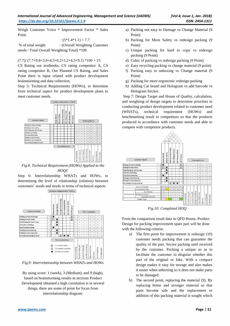
International Journal of Advanced Engineering, Management and Science (IJAEMS) [Vol-4, Issue-1, Jan- 2018]
https://dx.doi.org/10.22161/ijaems.4.1.9 ISSN: 2454-1311
www.ijaems.com Page | 51
Weigh Customer Voice * Improvement Factor * Sales
Point
: (5*1.4*1.1) = 7.7
% of total weight : (Overall Weighting Customer
needs / Total Overall Weighting Total) *100
:
(7.7)/ (7.7+9.8+3.9+4.5+6.2+5.2+4.3+9.1) *100 = 15
CS Rating our textbooks, CS rating competitor A, CS
rating competitor B, Our Planned CS Rating, and Sales
Point there is input related with product development
brainstorming and data collection.
Step 5: Technical Requirements (HOWs), to determine
from technical aspect for product development plans to
meet customer needs.
Fig.8. Technical Requirement (HOWs) Applied to the
HOQC
Step 6: Interrelationship WHATs and HOWs, to
determining the level of relationship (relation) between
customers’ needs and needs in terms of technical aspects
Fig.9: Interrelationship between WHATs and HOWs
By using score: 1 (week), 3 (Medium), and 9 (high),
based on brainstorming results in sections Product
Development obtained a high correlation is in several
things, there are some of point for focus from
interrelationship diagram:
a) Packing not easy to Damage vs Change Material (9
Point)
b) Packing for More Safety vs redesign packing (9
Point)
c) Unique packing for hard to copy vs redesign
packing (9 Point)
d) Cubic of packing vs redesign packing (9 Point)
e) Easy recycling packing vs change material (9 point)
f) Packing easy to unboxing vs Change material (9
Point)
g) Packing for more ergonomic redesign packing
h) Adding Car brand and Hologram vs add barcode vs
Hologram Sticker.
Step 7: Design Target and House of Quality, calculation,
and weighting of design targets to determine priorities in
conducting product development related to customer need
(WHATs), technical requirement (HOWs) and
benchmarking result to competitors so that the products
produced in accordance with customer needs and able to
compete with competitor products.
Fig.10: Completed HOQ
From the comparison result data in QFD House, Product
Design for packing improvement spare part will be done
with the following criteria:
a) The first point for improvement is redesign (10)
customer needs packing that can guarantee the
quality of the part. Secure packing until received
by the customer. Packing a unique so as to
facilitate the customer to disguise whether this
part of the original or fake. With a compact
design makes it easy for storage and also makes
it easier when unboxing so it does not make parts
to be damaged.
b) The second point, replacing the material (9). By
replacing better and stronger material so that
parts become safe and the replacement or
addition of this packing material is sought which

International Journal of Advanced Engineering, Management and Science (IJAEMS) [Vol-4, Issue-1, Jan- 2018]
https://dx.doi.org/10.22161/ijaems.4.1.9 ISSN: 2454-1311
www.ijaems.com Page | 52
makes it easier to recycle by avoiding the use of
Styrofoam.
c) The Third point for improvement is add Barcode
(9) and Hologram (9). This improvement uses
for increase trust customer because they already
buy original part. And this barcode can connect
to internet to check authenticity spare part
d) The Four point to improvement Redesign print
screen (7) and wrapping (7). After we ask to
customer and seller about these two issues we
find that customer and seller is doesn’t care
about this issue. The most important is quality of
part. Customer and supplier almost remove the
packing of spare parts and spare parts that are
damaged so the economic value is lost here.
With this data we can do by not using the use of
color print out carton and coated by plastic. This
is done by doing a comparison with competitor
spare parts where they also do the same thing.
Fig.11.Sample before Improvement
Fig.12. Sample Target Improvement
V. CONCLUSION
1. Based on a review of VOC's voice of customer. The
color of the packing is not very influential on packing.
Customers only want a more solid packing. The
easiest thing is to replace the thicker carton box
material called Flute. The process of replacing this
material will certainly increase the cost of packing
spare parts. But because the customer is not too
influential with the color packing, this can be done
budget transfer from print to a better material. By
replacing the packing material will look more solid
and more exclusive and this one of reasons customer
chose the product
2. Another improvement has to be done to change the
design from packing for easier unboxing process.
This seems often unthinkable. Impact from difficult
to unpacking the customer using sharp objects and
potential of spare part material to be damaged.
3. Other improvements by removing the installation
instructions (which in screen printing in packing).
The installation instructions are rarely used by the
customer because the spare part is usually installed in
the workshop. One of the improvements that can be
used by connecting the barcode code with website
online, if the customer wants to see the installation
process just by doing scan spare part and we can see
instruction on website.
VI. REFERENCES
[1] Wagner SM, Lindemann E. A case study-based
analysis of spare parts management in the
engineering industry. Production Planning &
Control: The Management of Operations. 2008;
19:397-407.DOI:
https://doi.org/10.1080/09537280802034554
[2] Vargas C.A, Cortes ME. Automobile spare-parts
forecasting: a Comparative study of time series
method. International Journal of Automotive and
Mechanical Engineering. 2017 Volume 14, issue
1pp. 3898-3912.
DOI:
https://doi.org/10.15282/ijame.14.1.2017.7.0317
[3] https://www.gaikindo.or.id/pasar-domestik-
mobil-indonesia-baik-45-persen-pada-2016
[4] http://jatim.tribunnews.com/2017/06/13/penjuala
n-spare-part-honda-lebihi-target-tahun-2017-
diprediksi-akan-meningkat-saat-h-7-lebaran
[5] Kocamanlar, E. (2008) “A Model Proposal about
the Effect of Packing in Fast Moving Consumer
Goods on the Purchasing Behavior”
Postgraduate Thesis, İstanbul, the Institute of
Science of the Technical University of İstanbul.
[6] Gökalp, F. (2007) “The Role of Packing in
Purchasing Behavior of Food Products” Ege
Academic Review, 7(1):79-97.
[7] Rundh, B. (2009) “Packaging Design: Creating
Competitive Advantage with Product Packaging”
British Food Journal, 111(9):988-1002.

International Journal of Advanced Engineering, Management and Science (IJAEMS) [Vol-4, Issue-1, Jan- 2018]
https://dx.doi.org/10.22161/ijaems.4.1.9 ISSN: 2454-1311
www.ijaems.com Page | 53
DOI:
https://doi.org/10.1108/00070700910992880
[8] İnce, M. (2010) “Analyzing the Effects of
Packing as a Communication Instrument on
Customer Choice” Postgraduate Thesis, İstanbul,
The University of Marmara, The Institute of
Science.
[9] Yıldız, O.E. (2010) “The Effect of Packing in
Creating Brand Awareness” Communication
Theories and Researches Magazine, 31:181-194.
[10] Deutsche Gesellschaft f¨ur Qualit¨at e.V.,
Frankfurt. (2001)QFD – Quality Function
Deployment, Berlin, Wien,Z¨urich: Beuth Verlag
GmbH.
[11] Klein B. (2012) QFD – Quality Function
Deployment-Konzept, Renningen: Expert Verlag
[12] Hales, R. and Staley, D. (1995) Mix target
costing, QFD for successful new products,
Marketing News, 29(1),
[13] Kauffmann, P., Unal, R., Fernandez, A. and
Keating C. (2000) A model for allocating
resources to research programs by evaluating the
technical importance and research productivity,
Engineering Management Journal, Vol.12, No.1,
5-8.
[14] Hauser, J. R. and D. P. Clausing, the House of
Quality, Harvard Business Review, May/June
1988.
[15] A Griffin and JR Hauser (1992) Patterns of
Communication among Marketing, Engineering
and Manufacturing, A Comparison between Two
New Product Teams, Management Science 38
(3), 360-373.
[16] Jaiswal (2012) Case Study on Quality Function
Deployment (QFD), ISSN: 2278-1684 Volume
3,Issue 6: 31
[17] Hamidullah, R. Akbar, S. Noor, W. Shah &
Inayatullah (2010) QFD as a Tool for
Improvement of Car Dashboard, University of
Engineering and Technology Peshawar, Pakistan,
Journal of Quality and Technology Management
Volume VI, Issue 1, June.: 1 - 3
[18] Goetsch, D.L. and Davis, S.B. (2010) Quality
Management for Organization Excellence,
6th_ed. Upper Saddle River, NJ: Pearson
Education Inc., pp. 296-311.
[19] Sun Cheng etc. Paper Packaging Structure
Design. Beijing: Light Industry Press; 2006.
DOI:10.1016/j.proenv.2011.09.

International Journal of Advanced Engineering, Management and Science (IJAEMS) [Vol-4, Issue-1, Jan- 2018]
https://dx.doi.org/10.22161/ijaems.4.1.10 ISSN: 2454-1311
www.ijaems.com Page | 54
Gravitational Model to Predict the Megalopolis
Mobility of the Center of Mexico Juan Bacilio Guerrero Escamilla, Sócrates López Pérez, Yamile Rangel Martínez, Silvia
Mendoza Mendoza*
*Academic Area of Sociology and Demography, Institute of Social Sciences and Humanities, Autonomous University of the
State of Hidalgo. Pachuca City, Hidalgo State,México. Kilometer 4.5, Pachuca / Actopan Road, San Cayetano Neighborhood,
P.C. 42084, Phone(51) 771-7172000 ext. 5200 to 5234.
Abstract— Since 1950, Mexico has presented an
accelerated migration process to the country’s capital,
Mexico City. Here is where new settlements emerged
increasing its population, and as a positive consequence,
employment improved together with provisions. This growth
occurred until the 1980s, when a conurbation happened
with some municipalities of the State of Mexico, creating the
Metropolitan Area of the Valley of Mexico. In the beginning
of the 21st century, new challenges arose with the
integration of more metropolitan areas in the states of
Mexico (Valley of Toluca), Hidalgo, Morelos, Puebla,
Tlaxcala and Queretaro.
This document is the result of two extensive research
projects that took place from 2008 to 2016, along with the
population institutions of the states that were integrated.
The objective was to demonstrate the existence of the
Megalopolis and its operation, based on a socio-
demographic model to understand its composition and
characteristics. However, when limited to demographic
variables, it was difficult to analyze its operation.
Therefore, the Gravitational Model was designed to
establish the great diversity of mobility relationships to
account for the functional composition. Thus, the
population mobility that commutes daily to the interior of
the Megalopolis will be the fundamental factor to explain its
operation.
Keywords— Mexico Megalopolis, Gravitational model,
Population mobility, Commuters model, Metropolitan
Areas of Mexico, Urbanization of cities of Mexico.
I. INTRODUCTION
In the last fifty years, Mexico has gone through a number of
demographic phenomena, including migration processes.
These have varied in intensity according to the time period
and great diversity in its forms, whether internal inter-
municipal, rural-urban, interstate and international. Internal
migration is highlighted, since it has been the main way to
define the setup of the current territory, the geographical
distribution of its population, the definition and composition
of its regions, the growth and consolidation of cities, and the
current relationship between urban-rural populations.
At the same time, these internal population movements have
been determinant factorsfor demographic dynamics,
changes in the country’s geographical distribution,
economic diversification, integration of employment
markets, and the population of big citiesthat have become
attraction centers of population migration [1].This
demographic phenomenon is no longer the movement of the
population from the countryside to the city.Now, migration
is taking place among various urban centers, reaching high
levels in the medium cities, generating mass displacements
from the center of the Megalopolis towards a new network
of intermediate cities and metropolitan areas of the states
surrounding Mexico City as well asthe Municipalities of the
State of Mexico [3].
1.1 Integration of Metropolitan Areas in Mexico
In Mexico, the form of settlement defined as Metropolitan
Areas (ZM as per its Spanish acronym for “Zona
Metropolitana”), is a phenomenon that has been very
dynamic,enabling to define population nucleithroughout the
country and exceeding the municipal and state limits. These
(ZM’s) are characterized by being an urban regionthat
includes a central nucleus linked to other smaller
conglomerates (cities or municipalities); these are
intertwined by sharing specific functions, such as industry,
services, commerce and culture. This implies the formation
of a system in which a central city establishes a network of
relations with other cities or municipalities, as well as
maintaining a high population density, where the size is
related to the group of municipal administrations that are
integrated [1].The ZM’swere starting points for the
emergence of large spaces of differentiated trading, its own
dynamics and resources, the application, design and
development of large investment projects in various sectors,

International Journal of Advanced Engineering, Management and Science (IJAEMS) [Vol-4, Issue-1, Jan- 2018]
https://dx.doi.org/10.22161/ijaems.4.1.10 ISSN: 2454-1311
www.ijaems.com Page | 55
and its own dominant center. ZM’s are linked to peripheries
and suburban spaces, with social groups and culture that
gives them their own identity. This leads us to conceptualize
the megalopolis of Mexico, beyond the simple integration
or absorption of small cities, with urban agglomerates,
emergence of suburbs, and dormitory cities or satellites.
The ZM with the largest population, majordynamism,
economy, mobility and integration of states and
municipalities, is the one that has been formed around
Mexico City [7].This ZM, under various demographic
processes, hasbeen growing at an accelerated rate in the last
decades of the last century. Thisleadsto new population
dynamics and changes in its various indicators, rates,
growth, displacement and migration [2].This urban region is
the sum of numerouscities that have been integrated.
According to their growth, an increasingly bigger area is
being formed, through nuclei that integrate millions of
inhabitants, grouped in different cities and with clear
relationships of functionality and trade. All of this is
forming a megacity, megalopolis or megapolis [4].
1.2. The Megalopolis
The term megalopolis is understood as those urban regions
that reach or surpass 10 million inhabitants, within the space
or territory occupied by several cities [5]. In some cases, it
is also defined when they have a population density of at
least 2,000 inhabitants per km2. However, the concept does
not stop there, the studies carried out during the 1960s on
large cities in North America defined Megalopolis in
broader terms, since it wasn’t limited to population
volumes, which led to an integration and functioning of a
wider body of cities and urban areas. The term megalopolis
was defined as the formation of a set of Metropolitan Areas,
whose accelerated urban growth leads to the contact of the
area of influence of one another. Thus, the megalopolis
usually consists of conurbations of large cities. This concept
also includes a Global City that according to its author
Saskia Sassen, applies to the cities that have a series of
characteristics. These characteristics are the result of
globalization and the constant growth of urbanization,
including its broader and more comprehensive forms as
political, economic and cultural categories.
The most common trend in the formation of a Megalopolis
is the urbanization of large territories that have different
ZM’s that are linked to a single urban system, characterized
by maintaining a dynamic interaction between two or more
ZM’s. The studymentioned previously, points outthatthese
areas are wealthy and productive, forming a new urban
system which houses the most prosperous andwell-educated
groups withaccess to social services [5].
1.3 Central Mexico area Megalopolis
One of the first proposals of the central Mexico
areamegalopolis was in 1976. Itestablishedthe existence of
12 metropolitan areas [15]within the context described by
the UN in 1966, by considering them as the territorial
extension that includes the political-administrative unit that
contains the central city, and the contiguous political-
administrative units that have urban characteristics such as
workplaces or residences of non-agricultural workers.
Also,they maintain a direct, constant and intense socio-
economic interrelationship with the central city and vice
versa [3].Later, inan analysis from the 1980s, the
Megalopolis was defined as the integration of 26
Metropolitan Areas, which included the 12 ZM’s of the
previous period [11], and defined the formation of the city
in a first stage, in which the population, as well as the
economic activity, housing and urban services tend to
concentrate in the center of the city. This is followed by a
second phase of physical expansion of the city and
expansion of its influence radius; suburbanization is
generated and new work centers and concentration of
services appear within the urban area. If, in this process, the
city absorbs one or more political-administrative units, close
and external, they will growaround it and with that, a
Metropolitan Area will appear [10].
In 1993, new areaswere aggregated to the territory.Jaime
Sobrino identified 37 metropolitan areas by pointing to the
metropolitan areas with contiguity and integration graphs.At
the same time, he integrated a statistic and applied the main
components method with the variables of demographic
growth rates, urbanization rate, GDP of the municipal
manufacturing industry and coverage of drinking water
services [14].
Recently, new proposals have been presented under a
delimitation, considering the urban character of the
municipality and the intermunicipality trips due to
commuting.In addition, the demographic dynamics and the
economic importance of the municipality are identified in48
Metropolitan Areas which population represented almost
half of the national population in the year 2000 [13].
The National Institute of Statistics Geography and
Informatics (INEGI, as per its Spanish acronym),marked 32
Metropolitan Areas integrated by 205 municipalities,
consideringthe size of the city and its relation of physical
contiguity, and also based on the cartography of the national
geostatistic framework and urban AGEB [6].

International Journal of Advanced Engineering, Management and Science (IJAEMS) [Vol-4, Issue-1, Jan- 2018]
https://dx.doi.org/10.22161/ijaems.4.1.10 ISSN: 2454-1311
www.ijaems.com Page | 56
In more recent studies, and following the international
urbanization trends, a metropolitan area is considered a
central place that remains as a political-administrative unit,
containing an urban area with 50 thousand or more
inhabitants. However, for any unit to be part of a
metropolitan area, it must be in territorial contiguity and
maintain certain physical-geographical, socioeconomic and
functional integration variables.
In 1995, the National Population Council (CONAPO, as per
its Spanish acronym)identified 31 Metropolitan Areas and
defined it as a set of two or more municipalities that
contained, within its boundaries, a city of 100 thousand or
more inhabitants, and whose population and productive
activities had urban characteristics.
In 2003, CONAPO identified 42 Metropolitan Areas,
integrated by243 municipalities, pointing to its definition,
the size and conurbation (physical union), the functional
integration related to the displacement of the employed
population between the municipalities of residence and
work, as well as criteria on the urban character of the
municipalities.
The Secretariat of Social Development (SEDESOL, as per
its Spanish acronym), based on the National Urban
Development Program 1990-1994, 1995-2000, 2001-2006;
specified that a Metropolitan Area was defined as “Those
city networks, where the metropolization processes that
involve cities of Mexico and the United States of America
or cities that have more than a million inhabitants”.
II. THEORETICAL FRAMEWORK AND
DEVELOPMENT OF THE GRAVITATIONAL
MODEL
In the report on Urban Poverty and Metropolitan Areas in
Mexico presented by the National Council for the
Evaluation of the Social Development Policy (CONEVAL,
as per its Spanish acronym) in 2013, a metropolitan area
was defined as a group of municipalities in a single unit
sharing a central city and that are functionally interrelated.
This concept was developed in the United States in the early
1920s and refers to a large city where its limits exceed the
political-administrative unit of a municipality. This process
of metropolization is understood as “the special dynamics
generated by the changes made in the production mode that
involves the trend association of city networks or urban
agglomerations constituting an urban conglomerate with
common characteristics: economic, social, functional and
productive, which define the flow of goods, people and
financial resources”.
Within the center of the country’smetropolitan areas,
continuous displacements of the population are generated,
which are known as commuting.That is to say, it is the
travel done by the inhabitants of a metropolitan area from
their place of residence to their destination, where the
intensities of displacements provide elements to determine
the strength that drives the city’s growth.
A City is defined as an agglomeration that includes
considerable extensions that surpass its limits and that were
historically marked by a past political decision. At present,
cities in metropolitan areas at the center of the country
expand beyond their original administrative area, reaching
spaces of other cities, forming a large metropolitan area that
exceeds its administration.
In this context, metropolitan areas reach a depletion limit in
the proper use of their resources, which causes major
problems, such as an inefficient infrastructure with low
maintenance, low tax collection, increased insecurity and
excess pollution. These problems result in continuous
population displacements among the different metropolitan
areas, resulting in an economic and social dynamic where
mobility is related with a cost-benefit analysis.
Based on the above, the population mobility experienced in
the metropolitan areas of the center of the country is the
result of the economic and social growth that these regions
have developed over time. This element gives rise to the
need to measure the magnitude of mobility among the
different areas. Therefore, this document has a theoretical
basis in the gravitational law, because by its application it
will be possible to predict the dynamics of the inhabitants
commuting, and with this, measure the degree of specialty,
by identifying the benefits and difficulties that each one of
them currently present.
The gravitational law (2ndlaw of Issac Newton, 1642-1727)
is part of mechanical physics and aims to describe the
gravitational interaction between different bodies with
mass. Newton demonstrated that the force of gravity has the
direction of the line that connects the centers of the stars
and the direction corresponds to an attraction [9].
Newton discovered that the force of attraction of two bodies
is expressed as follows:
F⃗ = |G|M ∗ m
R2 (1)
Where:
F⃗ is the foce exerted between both
bodies.
M is the mass of attraction of
object one.
m is the mass of attraction of
object two.
R is the distance that exists

International Journal of Advanced Engineering, Management and Science (IJAEMS) [Vol-4, Issue-1, Jan- 2018]
https://dx.doi.org/10.22161/ijaems.4.1.10 ISSN: 2454-1311
www.ijaems.com Page | 57
between both objects.
G is the universal gravitation
constant.
Equation (1) means the following:
“The force of gravity between two bodies is proportional to
the product of their masses and inversely proportional to
their square distance”
Fig.1: Graph of force of attraction between two bodies.
Source. Own elaboration, México, 2017.
That is, the greater the weight of the masses of both bodies,
the greater their attraction, but this will depend on the
distance between them, therefore we assume the following
[8]:
- The greater weight of the mass between the bodies,
the greater force of attraction.
- The smaller the distance between the bodies, the
greater force of attraction.
Based on the above, the attraction force of one Metropolitan
Area with respect to another will depend on the weight of
their masses and inversely proportional to the distances and
the time needed to cover those distances (Figure2).
Fig.2: Graph of the force of attraction of two metropolitan areas.
Source. Own elaboration, México, 2017.
That is:
“The force of attraction between two metropolitan areas is
proportional to their masses, and inversely proportional to
the square of their distance”
Therefore, from the theory of gravitational law, the force of
attraction of two Metropolitan Areas is expressed as
follows:
FAi = [(Mi)(Mj)
(di)2
] ∗ 100; FAi ∈ ℛ+; i ≠ j (2)
Where:
- FAi is the rate of the force of attraction between the
i-th metropolitan area and the j-th metropolitan
area.
- Mi is the attraction mass of the i-thmetropolitan
area.
- Mj is the attraction mass of the j-th metropolitan
area.
- di is the distance between the i-th metropolitan
area and the j-th metropolitan area (Km).
The dynamic mobility rate (commuting)of the i-th
Metropolitan Area in relationto the others is expressed as
follows:
FATi = ∫FAi
10
a
b
dPA ~ √∏FAi
10
𝑖=1
10
; FAi
∈ ℛ+ (3)
Its interpretation is as follows:
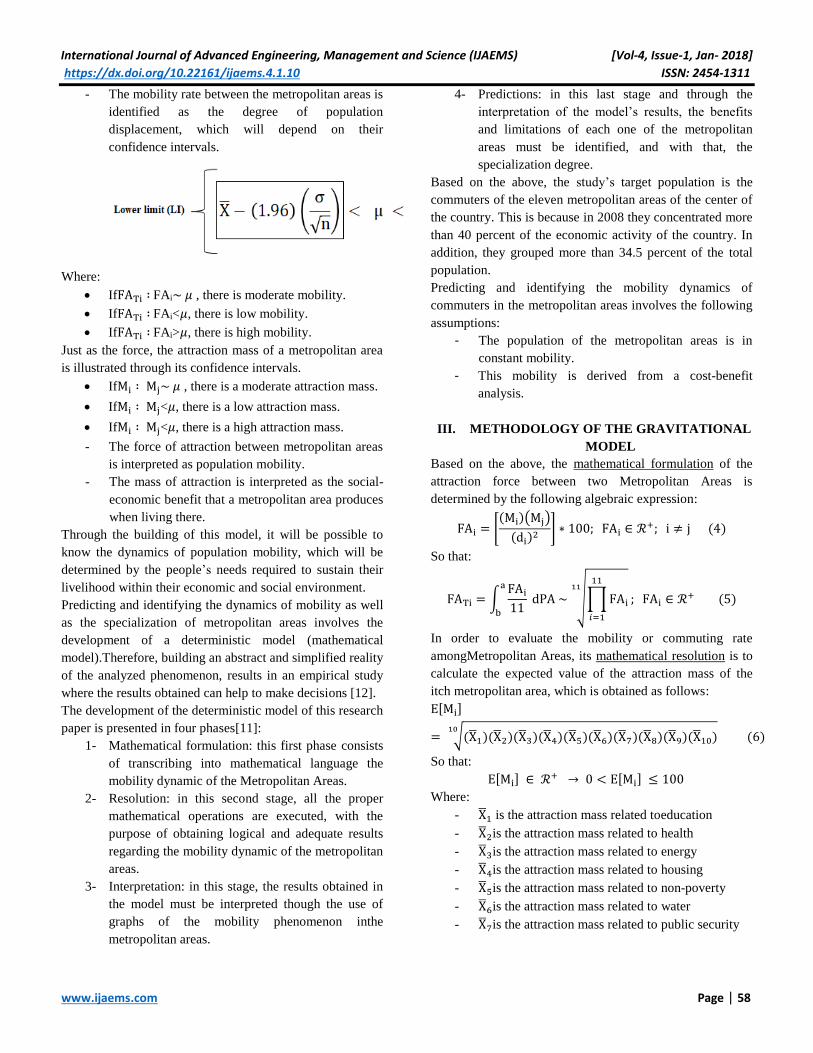
International Journal of Advanced Engineering, Management and Science (IJAEMS) [Vol-4, Issue-1, Jan- 2018]
https://dx.doi.org/10.22161/ijaems.4.1.10 ISSN: 2454-1311
www.ijaems.com Page | 58
- The mobility rate between the metropolitan areas is
identified as the degree of population
displacement, which will depend on their
confidence intervals.
Where:
IfFATi ∶ FAi~ 𝜇 , there is moderate mobility.
IfFATi ∶ FAi<𝜇, there is low mobility.
IfFATi ∶ FAi>𝜇, there is high mobility.
Just as the force, the attraction mass of a metropolitan area
is illustrated through its confidence intervals.
IfMi ∶ Mj~ 𝜇 , there is a moderate attraction mass.
IfMi ∶ Mj<𝜇, there is a low attraction mass.
IfMi ∶ Mj<𝜇, there is a high attraction mass.
- The force of attraction between metropolitan areas
is interpreted as population mobility.
- The mass of attraction is interpreted as the social-
economic benefit that a metropolitan area produces
when living there.
Through the building of this model, it will be possible to
know the dynamics of population mobility, which will be
determined by the people’s needs required to sustain their
livelihood within their economic and social environment.
Predicting and identifying the dynamics of mobility as well
as the specialization of metropolitan areas involves the
development of a deterministic model (mathematical
model).Therefore, building an abstract and simplified reality
of the analyzed phenomenon, results in an empirical study
where the results obtained can help to make decisions [12].
The development of the deterministic model of this research
paper is presented in four phases[11]:
1- Mathematical formulation: this first phase consists
of transcribing into mathematical language the
mobility dynamic of the Metropolitan Areas.
2- Resolution: in this second stage, all the proper
mathematical operations are executed, with the
purpose of obtaining logical and adequate results
regarding the mobility dynamic of the metropolitan
areas.
3- Interpretation: in this stage, the results obtained in
the model must be interpreted though the use of
graphs of the mobility phenomenon inthe
metropolitan areas.
4- Predictions: in this last stage and through the
interpretation of the model’s results, the benefits
and limitations of each one of the metropolitan
areas must be identified, and with that, the
specialization degree.
Based on the above, the study’s target population is the
commuters of the eleven metropolitan areas of the center of
the country. This is because in 2008 they concentrated more
than 40 percent of the economic activity of the country. In
addition, they grouped more than 34.5 percent of the total
population.
Predicting and identifying the mobility dynamics of
commuters in the metropolitan areas involves the following
assumptions:
- The population of the metropolitan areas is in
constant mobility.
- This mobility is derived from a cost-benefit
analysis.
III. METHODOLOGY OF THE GRAVITATIONAL
MODEL
Based on the above, the mathematical formulation of the
attraction force between two Metropolitan Areas is
determined by the following algebraic expression:
FAi = [(Mi)(Mj)
(di)2
] ∗ 100; FAi ∈ ℛ+; i ≠ j (4)
So that:
FATi = ∫FAi
11
a
b
dPA ~ √∏FAi
11
𝑖=1
11
; FAi ∈ ℛ+ (5)
In order to evaluate the mobility or commuting rate
amongMetropolitan Areas, its mathematical resolution is to
calculate the expected value of the attraction mass of the
itch metropolitan area, which is obtained as follows:
E[Mi]
= √(X̅1)(X̅2)(X̅3)(X̅4)(X̅5)(X̅6)(X̅7)(X̅8)(X̅9)(X̅10)10
(6)
So that:
E[Mi] ∈ ℛ+ → 0 < E[Mi] ≤ 100
Where:
- X̅1 is the attraction mass related toeducation
- X̅2is the attraction mass related to health
- X̅3is the attraction mass related to energy
- X̅4is the attraction mass related to housing
- X̅5is the attraction mass related to non-poverty
- X̅6is the attraction mass related to water
- X̅7is the attraction mass related to public security

International Journal of Advanced Engineering, Management and Science (IJAEMS) [Vol-4, Issue-1, Jan- 2018]
https://dx.doi.org/10.22161/ijaems.4.1.10 ISSN: 2454-1311
www.ijaems.com Page | 59
- X̅8is the attraction mass related to transportation
and infrastructure
- X̅9is the attraction mass related to non-
contamination
- X̅10is the attraction mass related toemployment
The expected value of anyX̅i is obtained by standardizing
the information through logarithms.
The estimation and interpretation of the results of the
present model are structured from two aspects:
1- The prediction of the mobility dynamics of
commuters of metropolitan areas, taking each one
of their attraction massesas a reference.
2- The measurement and identification of the
specialty of each one of the metropolitan areas,
derived fromthe mobility dynamics of commuters.
By reading these results, it will be possible to make
projections onthe socio-economic trend that each one of the
metropolitan areas must follow, which will provide the
necessary elements to propose a megalopolitan
management, with the purpose of obtaining a better
distribution of the economic resources that each one of them
generates.
Themobility dynamics of the metropolitan areas will be
interpreted as the commuting degree that the inhabitants of
each area are willing to experience.
Fig.3: Mobility degree per Metropolitan Area.
Source. Own elaboration, México, 2017.
Based on figure4, it can be seen that the Tianguistenco and
Toluca areas experience a high degree of mobility (61 and
51 units), when compared to the others. On the other hand,
Tula and Queretaro are the ones with less mobility, while
the other areas have a homogeneous behavior.
Example: the mobility rate of all the
Metropolitan Areas is 29.50 units:
FATi = √∏FAi
11
𝑖=1
11
= √(61)(51.03)(35.53)(34)(32.08)(31.94)(31.22)(30.28)(25.55)(19.08)(8.36)11
Therefore:
FATi = √∏FAi
11
i=1
11
= 29.50 units
Where:
- FAi is the expected value of the attraction in
the i-th attraction mass, which is obtained
from the following algebraic expression:
FAi = [(Mi)(Mj)
(di)2
] ∗ 100; FAi ∈ ℛ+; i ≠ j
The masses drivingthe mobility of all the metropolitan areas
are the following (figure 5):
- Housing. As a social entity, it is the place where
the family settles, lives, grows and thrives.
Therefore, it is the economic and social
development of the individual [3].

International Journal of Advanced Engineering, Management and Science (IJAEMS) [Vol-4, Issue-1, Jan- 2018]
https://dx.doi.org/10.22161/ijaems.4.1.10 ISSN: 2454-1311
www.ijaems.com Page | 60
Fig.4: Rank of majorinfluence masses in the commuting amongthe metropolitan areas inthe center of the country. Source. Own
elaboration, México, 2017.
- Education:The tool must transmit knowledge,
values, customs, behaviors, attitudes and course of
actions that the human being must acquire and use
throughout their life.
- Water: it is the most important non-renewable
resource for the survival of any living being. This
resource gave rise to life and it sustains it; it is a
factor that regulates the planet’s weather.It creates
and allows the existence of ecosystems and
mankind.
Meanwhile, health, transportation, infrastructure,
employment quality, and the fight against poverty generate
a moderate mobility, probably due to the following factor:
the gap between these attraction masses of each
metropolitan area is not very wide.This is presumably
because of the living costs in each one of them. Most likely,
the Valley of Mexico offers better quality jobs than any
other Metropolitan Area, however the costs of livingthere is
more expensive than the others.Therefore, a person would
have to make a cost-benefit analysis on employment.
On the other hand, in spite of the increase of the
environmental and insecurity issues throughout the country,
they are notstill elements that strongly detonate population
mobility amongthe metropolitan areas.
Based on the above and according to figure 6, the
metropolitan area that generates more attraction force is
Queretaro, due to four factors (figure 6): highly qualified
jobs, low poverty rates, efficiency in energy supply,
transportation and infrastructure.

International Journal of Advanced Engineering, Management and Science (IJAEMS) [Vol-4, Issue-1, Jan- 2018]
https://dx.doi.org/10.22161/ijaems.4.1.10 ISSN: 2454-1311
www.ijaems.com Page | 61
Fig.5: Expulsion and attraction per Metropolitan area.
Source. Own elaboration, México, 2017.
In the example, the mobility rate of all the
Metropolitan Areas was 29.50 units,
therefore, the attraction force between them
would be70.50 units
Therefore:
FATi = √∏FAi
11
i=1
11
= 29.50 units → FATj = 100 − FATi
= 100 − 29.50 = 70.50 units
In addition, education, health, water, public security and
garbage collection behave similarly to the other
metropolitan areas (except for Puebla-Tlaxcala and the
Valley of Mexico, because in education and health they are
above Queretaro). Their main limitation is house acquisition
due to rising home prices as a result of the cost of living
increment in the area.
The second metropolitan area with greater attraction is Tula
due to two factors:
- It ranks 3rdin offering the best jobs because the
Miguel Hidalgo refinery and the Fortaleza cement
factory are located within its territory. Also, it has
one of the most important archeological areas in
the state of Hidalgo.
- Tula presents a moderate attraction force in
education, health, energy, housing, water supply,
public security, transportation, infrastructure, and
fight against poverty. However, currently it has
major issues with garbage collection which
contributes to the high pollution rates. Most of the
pollution comes from the Miguel Hidalgo refinery
and the Fortaleza cement factory.

International Journal of Advanced Engineering, Management and Science (IJAEMS) [Vol-4, Issue-1, Jan- 2018]
https://dx.doi.org/10.22161/ijaems.4.1.10 ISSN: 2454-1311
www.ijaems.com Page | 62
Fig.6: Boxplot of attraction force per Metropolitan area by mass of attraction.
Source. Own elaboration, México, 2017.
The metropolitan area of Tulancingo is in third place in
attraction force due to three factors:
- Housing acquisition cost is low; therefore, it is the
largest mass of attraction within the Area.
- Its garbage collection system is efficient.
- It has a homogeneous behavior compared to the
other areas in education, health, employment,
public transportation and infrastructure, public
security, water, energy, and fight against poverty.
The metropolitan area of Tlaxcala –Apizaco presents a force
of attraction of 69.72 units. This is because health,
education, employment, public transportation and
infrastructure, public security, water and fight against
poverty present a similar behavior to other areas, except for
Puebla-Tlaxcala, Valley of Mexico and Queretaro that are
significantly superior in education, health, employment,
public transportation and infrastructure. Therefore, the
mobility experienced by their inhabitants will be towards
those areas. Its main weakness is energy supply.
For the metropolitan area of Pachuca, its attraction force is
of 68.78 units due to the following:
- Its greatest strength is housing, as acquisition costs
are much lower than all other areas.
- It has a moderate behavior in education, health,
energy, transportation, infrastructure, garbage
collection, employment quality, and fight against
poverty. However, in education, health, energy and
fight against poverty it is surpassed by the Valley
of Mexico, Puebla-Tlaxcala and Queretaro.
- In public security, it is vastly superior to
Cuernavaca and the Valley of Mexico.
- Its transportation and infrastructure is more
efficient than Tulancingo’s, but inferior to the
Valley of Mexico, Toluca and Queretaro.
- In garbage collection, it is more efficient than Tula
and the Valley of Mexico, however, it is surpassed
by Tianguistenco and Tulancingo.
- Its employment quality is inferior to Queretaro,
Valley of Mexico and Tula.
The Metropolitan Area of Cuernavaca, has an attraction
force of 68.06 unitsdue to the following:
- Its main strength is water supply, ranked just
below the metropolitan area of Puebla (top
position)
- It has moderate behavior in education, health,
energy, housing, transportation and infrastructure,
garbage collection, and employment quality.
- Regarding education and health, it is surpassed by
the Valley of Mexico and Puebla-Tlaxcala.
- In the energy supply, it is inferior to the Valley of
Mexico and Queretaro.
- Its housing cost is moderate, however, it is
surpassed by Pachuca and Tulancingo.

International Journal of Advanced Engineering, Management and Science (IJAEMS) [Vol-4, Issue-1, Jan- 2018]
https://dx.doi.org/10.22161/ijaems.4.1.10 ISSN: 2454-1311
www.ijaems.com Page | 63
- Transportation and infrastructure have better
quality in the Valley of Mexico, Toluca and
Queretaro.
- Its garbage collection system is less efficient than
Tianguistenco and Tulancingo.
- Their employment quality is inferior to Queretaro,
Valley of Mexico and Tula.
For the metropolitan area of Cuautla, its force of attraction
is 67.92 units and this behavior is due to the fact that its
attraction masses exhibit a moderate behavior.However, the
mobility of its population (32.08 units) is due to the
following factors:
- In education, health and energy it is surpassed by
the Valley of Mexico, Puebla-Toluca
andQueretaro.
- The cost of housing is above Pachuca and
Tulancingo, however, it is inferior to Queretaroand
the Valley of Mexico.
- In the fight against poverty, it is more efficient
than Toluca, but inferior to Queretaro.
- Its water supply is more efficient than that of
Toluca, but less efficient than that of Puebla-
Tlaxcala and Cuernavaca.
- In public security it is above Cuernavaca and the
Valley of Mexico, and below Tianguistenco.
- Public transportation and infrastructure is more
efficient than that of Tulancingo, however, it is
below Queretaro, the Valley of Mexico and
Toluca.
- Its garbage collection system is better than the
Valley of Mexico and Tula, but inferior to
Tianguistenco and Tulancingo.
- The employment quality does not compare to the
Valley of Mexico, Queretaro and Tula, however, it
is comparable with the other metropolitan areas,
except for Tianguistenco.
The metropolitan area of the Valley of Mexico has an
attraction force of 66 units due to the high indicators in
education, health, energy, transportation and infrastructure,
and employment quality but inferior to Queretaro’s. Its
main weaknesses are the high cost of housing, the public
security system and the way garbage is collected. These
indicators are also supported by data provided by INEGI in
2015. This showed that the activity with the highest
prevalence in the Valley of Mexico is the tertiary sector
(education, health and finance, among others),
concentrating 66.27 percent of all activities.
For the metropolitan area of Puebla–Tlaxcala its attraction
force is 64.77 units as a consequence of the great benefits it
offers in education, health and water supply (the Valley of
Mexico is the only Area that surpasses it in education and
health).Its other attraction masses present a moderate
behavior, however, there are some areas that surpass it:
- In energy and housing by the Valley of Mexico,
Pachuca and Tulancingo.
- In the fight against poverty by Queretaro.
- In public security by Tianquistenco but it is widely
superior than Cuernavaca and the Valley of
Mexico.
- In transportation and infrastructure, the Valley of
Mexico, Toluca andQueretaroare superior.
- In garbage collection by Tianguistenco and
Tulancingo.
- Employment quality by the Valley of Mexico,
Queretaroand Tula.
The metropolitan areas with lower attraction force are
Toluca and Tianguistenco (48.97 and 39.00 units):
- Toluca’s attraction force is determined by the
following:
Its strength in public transportation and
infrastructure.
Its limitations in education, health, water
supply, energy, and employment quality.
In public security and garbage collection
it is moderate, however, it is inferior to
Tianguistenco and Tulancingo.
- The force of attraction of Tianguistenco is
determined by:
Its strength in public security and garbage
collection.
Its weaknesses in education, health and
quality of employment.
It shows a moderate behavior in public
transportation, infrastructure, water,
energy and housing
Based on the analysis of the results of all metropolitan
areas, the prediction of this model focuses on the
specializationof each area (Table1):
- The Valley of Mexico specializes in education,
health, transportation, infrastructure and quality
employment. However, it presents major problems
in house acquisition and public security.
- Queretaro specializes in the highest paid jobs
among all the Metropolitan Areas. Also, a high
specialization in efficiency of transportation and

International Journal of Advanced Engineering, Management and Science (IJAEMS) [Vol-4, Issue-1, Jan- 2018]
https://dx.doi.org/10.22161/ijaems.4.1.10 ISSN: 2454-1311
www.ijaems.com Page | 64
infrastructure, energy supply, and the fight against
poverty.
- Tula specializes in creating well-paid jobs, as a
result of the electric and cement industries, as well
as the tourism in its archaeological area.
- Pachuca specializes mainly in housing due to its
low acquisition cost. Just like Pachuca and
Tulancingo specialize in housing.
- Tlaxcala-Apizaco has a moderate specialization,
since the majority of its attraction masses have an
impartial behavior, except for energy supply.
- Puebla-Tlaxcala specializes in education, health
and water.
- Cuautla has a moderate specializationin all its
attraction masses.
- Cuernavaca specializes in water supply, however,
it faces major insecurity problems.
- Toluca specilizes in public transportation and
infrastructure, however, its weakness is the fight
against poverty and water supply.
- Tianguistenco specializes in garbage collection and
public safety, however, it has too many limitations
in education, health and employment quality.
As it can be seen, building and developing a gravitational
model based onthe mobility of metropolitan areas gives us
the necessary elements to affirm where each one of them is
economically heading, and with that, making decisions on
how to manage and guidethe central area of the country.
Table.1: Specialization of each Metropolitan Area.
METROPOLIT
ANAREA
Education Healt
h
Energ
y
Housing Well-
being
Water Public
Security
Transportati
on
Infrastructur
e
Garbage
management
Employmen
t quality
Valley of Mexico
Queretaro
Tula
Pachuca
Tulancingo
Tlaxcala -
Apizaco
Puebla - Tlaxcala
Cuautla
Cuernavaca
Toluca
Tianguistengo
High
Specialization
Moderate
Specialization Low Specialization
Source. Own elaboration, México, 2017.
IV. CONCLUSION
Through the application of the gravitational model, it was
observed that the mobility of all the metropolitan areas in
the center of the country is 29.50 units, that is to say, 30 of
every 100 inhabitants commute. Specifically, the main
drivers are housing, education and water. In addition, its
attraction force is 70.50 (71 of every 100 inhabitants have
the intention of moving within the center of the country).
The metropolitan area of Queretaro is the one that
experiences less population mobility. Moreover, it is the one
that generates the greatest attraction force compared to the
others, since it offers the best paying jobs in the center of
the country. This causesa reduction on their poverty

International Journal of Advanced Engineering, Management and Science (IJAEMS) [Vol-4, Issue-1, Jan- 2018]
https://dx.doi.org/10.22161/ijaems.4.1.10 ISSN: 2454-1311
www.ijaems.com Page | 65
indicators. In addition, they have built a solid infrastructure
resulting in awider distribution of their wealth. Regarding
the population mobility, the metropolitan area of
Tianguistenco presents the greatest population mobility and
the lowest attraction force, because it has limitations in
education, health and employment quality. Its main virtues
are public security and garbage collection.
Based on the most influential masses in commuting
(housing, education and water), the following could be
identified: the metropolitan areas of the Valley of Mexico
and of Puebla-Tlaxcala are the ones that offer better
education centers, since both have higher education
institutions (UNAM, IPN, CIDE, COLMEX, UDLA,
BUAP, and UPAEP, among others).In health, just as in
education, both areas are the most prominent in the center
of the country, since they have important medical centers
(Hospital Angeles, Hospital la Raza, Asociación Nacional
de Hospitales Privados, Hospital Universitario BUAP,
Hospital Puebla, and Sociedad de Beneficencia Española,
among others).In water, the model predicted that the
metropolitan areas of Puebla – Tlaxcala and Cuernavaca
present better efficiency in the water supply. This stresses
the importance of optimizing the water consumption and
reducing the contamination throughout the socio-economic
activities.
Other relevant results from the present model are the
security problems that are collectively presented in the
metropolitan areas, and to a greater extent in the Valley of
Mexico and Cuernavaca. This phenomenon most likely
stems from the lack of institutional, political and social
agreements related to the functions of the different public
powers, because in their absence, there is no link between
the public security system and citizens. Therefore, a system
is formed where corruption and impunity prevail.
In addition, the employment quality in most of the
metropolitan areas is low except for the Valley of Mexico
and Queretaro. This behavior is due to the low economic
activity, as the result of the low labor productivity. In other
words, there is not enough skilled labor, therefore, wages
are low. As a consequence, there is little private investment.
REFERENCES
[1] CONAPO; SEDESOL; INEGI. (2012), Delimitation of
Metropolitan Areas of Mexico 2010. National
Population Council (CONAPO), Ministry of Social
Development (SEDESOL), National Institute of
Statistics and Geography (INEGI), Mexico.
[2] CORONA, Reina, & Luque, Rodolfo. (1992), "Recent
Changes in Migration Patterns to the Metropolitan
Area of Mexico City (ZMCM)", Demographic and
Urban Studies, vol. 7, no. 2-3, Mexico.
[3] FLORES, Sergio. (2002), "Urban planning and
sustainable regional development in the metropolitan
area of Puebla-Tlaxcala" in Delgadillo, Javier,
Iracheta, Alfonso, Current regional research in Central
Mexico, CRIM, UNAM, Mexico, pp. 195-220.
[4] FORSTALL, Richard. (2004), Which Are The
Largest? Why Published Populations For Major World
Urban Areas Vary So Greatly, Consultant, Richard P.
Greene, Northern Illinois University, James B. Pick,
University of Redlands, United Kingdom.
[5] GOTTMANN, Jean. (1961), Megalopolis: The
Urbanized Northeastern Seaboard of the United States.
Editor Literary Licensing ISBN 1258423251,
9781258423254
[6] INEGI. (2002), Statistical Notebooks of the
Metropolitan Area of Mexico City. Edition 2002.
National Institute of Statistics and Geography
(INEGI), Mexico.
[7] LOPEZ, Socrates. (2009), Sociodemographic
diagnosis of the megalopolis of the center of the
country. Autonomous University of the State of
Hidalgo, Mexico, pp. 200.
[8] MARTÍN, I. (2004). General Physics. Spain:
University of Valladolid.
[9] MEDINA, A. and Ovejero, J. (2011). Newton's laws
and their applications. Spain: University of Salamanca.
[10] NEGRETE, María, & Salazar, Héctor. (1986).
"Metropolitan areas in Mexico, 1980", in Estudios
Demográficos y Urbanos, vol. 1, no. 1, The College of
Mexico, Mexico.
[11] RÍOS, S. (1995). Modeling Spain: Editorial alliance.
[12] RODRÍGUEZ, J. (2010). Mathematical models. Spain:
Open University of Catalonia.
[13] SOBRINO Jaime, (1993), "Government and
metropolitan and regional administration", National
Institute of Public Administration, A. C., Mexico.
[14] SOBRINO Jaime, (2003), "Delimitation of the
metropolitan areas of Mexico in 2000", in the National
Population Council (coord.), The delimitation of
zones, metropolitan, Mexico, CONAPO, SEDESOL,
INEGI, Institute of Geography-UNAM, Mexico, pp.
121-151.
[15] UNIKEL, Luis. (1976), Urban development in
Mexico, diagnosis and future implications. The
College of Mexico, Mexico, pp. 116
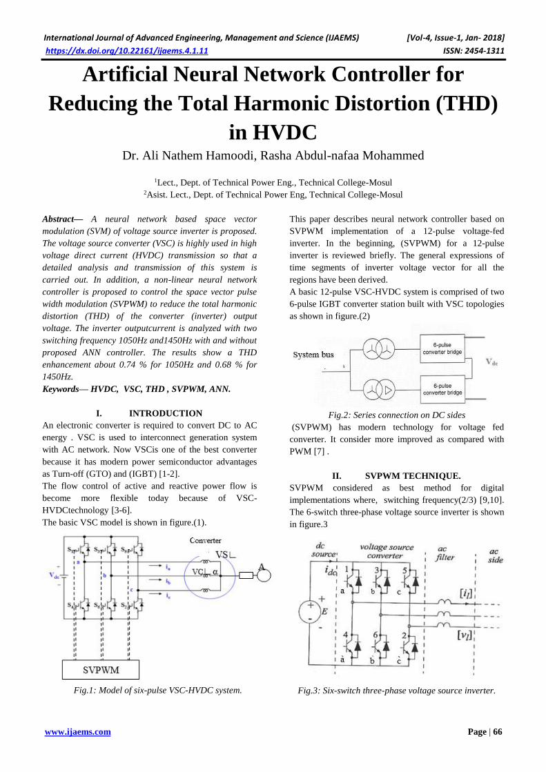
International Journal of Advanced Engineering, Management and Science (IJAEMS) [Vol-4, Issue-1, Jan- 2018]
1311-ISSN: 2454 https://dx.doi.org/10.22161/ijaems.4.1.11
66| Page www.ijaems.com
Artificial Neural Network Controller for
Reducing the Total Harmonic Distortion (THD)
in HVDC Dr. Ali Nathem Hamoodi, Rasha Abdul-nafaa Mohammed
1Lect., Dept. of Technical Power Eng., Technical College-Mosul
2Asist. Lect., Dept. of Technical Power Eng, Technical College-Mosul
Abstract— A neural network based space vector
modulation (SVM) of voltage source inverter is proposed.
The voltage source converter (VSC) is highly used in high
voltage direct current (HVDC) transmission so that a
detailed analysis and transmission of this system is
carried out. In addition, a non-linear neural network
controller is proposed to control the space vector pulse
width modulation (SVPWM) to reduce the total harmonic
distortion (THD) of the converter (inverter) output
voltage. The inverter outputcurrent is analyzed with two
switching frequency 1050Hz and1450Hz with and without
proposed ANN controller. The results show a THD
enhancement about 0.74 % for 1050Hz and 0.68 % for
1450Hz.
Keywords— HVDC, VSC, THD , SVPWM, ANN.
I. INTRODUCTION
An electronic converter is required to convert DC to AC
energy . VSC is used to interconnect generation system
with AC network. Now VSCis one of the best converter
because it has modern power semiconductor advantages
as Turn-off (GTO) and (IGBT) [1-2].
The flow control of active and reactive power flow is
become more flexible today because of VSC-
HVDCtechnology [3-6].
The basic VSC model is shown in figure.(1).
Fig.1: Model of six-pulse VSC-HVDC system.
This paper describes neural network controller based on
SVPWM implementation of a 12-pulse voltage-fed
inverter. In the beginning, (SVPWM) for a 12-pulse
inverter is reviewed briefly. The general expressions of
time segments of inverter voltage vector for all the
regions have been derived.
A basic 12-pulse VSC-HVDC system is comprised of two
6-pulse IGBT converter station built with VSC topologies
as shown in figure.(2)
Fig.2: Series connection on DC sides
(SVPWM) has modern technology for voltage fed
converter. It consider more improved as compared with
PWM [7] .
II. SVPWM TECHNIQUE.
SVPWM considered as best method for digital
implementations where, switching frequency(2/3) [9,10].
The 6-switch three-phase voltage source inverter is shown
in figure.3
Fig.3: Six-switch three-phase voltage source inverter.
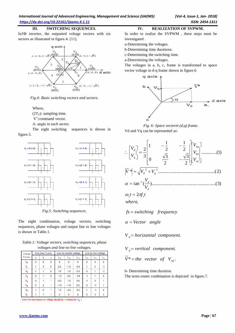
International Journal of Advanced Engineering, Management and Science (IJAEMS) [Vol-4, Issue-1, Jan- 2018]
1311-ISSN: 2454 https://dx.doi.org/10.22161/ijaems.4.1.11
67| Page www.ijaems.com
III. SWITCHING SEQUENCES.
In3Ф inverter, the outputted voltage vectors with six
sectors as illustrated in figure.4. [11].
Fig.4: Basic switching vectors and sectors.
Where,
(2TZ): sampling time.
V*:command vector.
Α: angle in each sector.
The eight switching sequences is shown in
figure.5.
Fig.5: Switching sequences.
The eight combination, voltage vectors, switching
sequences, phase voltages and output line to line voltages
is shown in Table.1.
Table.1: Voltage vectors, switching sequences, phase
voltages and line-to-line voltages.
IV. REALIZATION OF SVPWM.
In order to realize the SVPWM , three steps must be
investigated .
a-Determining the voltages.
b-Determining time durations.
c-Determining the switching time.
a-Determining the voltages.
The voltages in a, b, c, frame is transformed to space
vector voltage in d-q frame shown in figure.6
Fig. 6: Space vectorin (d,q) frame.
Vd and Vq can be represented as:
.*
.
.
,
2
)3.....(........................................).........(tan
)2........(........................................*
)1...(..........
2
3
2
30
2
1
2
11
3
2
1
22
ref
d
d
ss
d
q
qd
cn
bn
an
q
d
VofvectortheV
componentverticalV
componenthorizantalV
angleVector
frequencyswitchingfs
where
tft
V
V
VVV
V
V
V
V
V
b- Determining time duration.
The terns router combination is depicted in figure.7.

International Journal of Advanced Engineering, Management and Science (IJAEMS) [Vol-4, Issue-1, Jan- 2018]
1311-ISSN: 2454 https://dx.doi.org/10.22161/ijaems.4.1.11
68| Page www.ijaems.com
Fig.7: Reference vector combination.
The switching time duration atany sector is determine by
the following equations:[12].
)6........(..........
600
61,(
61,(
),(
)5.....(..........................................................................................
3
1.
3
1.
*..3
3
1*.3
)4.........(..........33
*.3
3
*..3
3
1
3
*..3
210
2
1
toSectoristhat
throughnwhere
TTTT
nCosSin
nSinCos
Vdc
VT
nSin
Vdc
VTT
Sinn
CosCosn
SinVdc
VT
nSin
Vdc
VT
nSin
Vdc
VTT
z
z
z
z
z
z
Where,
T1, T2and T0 : is the time duration for each sector.
Tz:is the sampling time ( inverse of the switching
frequency (fs)).
c-Determining the switching timeof each transistor (S1 to
S6). The switching times of the upper and lower
transistors for each sector is shown in figure.8
Fig. 8: PWM patterns at each sector.

International Journal of Advanced Engineering, Management and Science (IJAEMS) [Vol-4, Issue-1, Jan- 2018]
1311-ISSN: 2454 https://dx.doi.org/10.22161/ijaems.4.1.11
69| Page www.ijaems.com
V. SIMULATION WITHOUT ANN IMPLICATION VSI-HVDC BASED SVPWM.
Figure.9 presents Matlab/Simulinkmodel of a 12-pluse VSI-HVDC based on SVPWM.
Fig.9: MATLAB/SIMULINK model of a VSI-HVDC on SVPWM.
The THD ratio of the line current for switching
frequencies1050Hz and 1450Hz is shown in figure. 10.
Fig.10: THD ratio of line current in time domain.
(a) at switching frequency (1050Hz).
(b) at switching frequency (1450Hz).
The THD ratio of the line to line voltage at 1050Hz and
1450Hz switching frequency is shown in figure.11.
Fig.11: THD ratio of line to line voltage in time domain.
(a) at switching frequency (1050Hz).
(b) at switching frequency (1450Hz).
The THD ratio of theline current and line-line voltage
shown in Table.2 are obtained directly by computer from
figures 10 & 11.
Table.2: THD values for line current and line to line
voltage
Switching
frequency(Hz)
Line current
THD value(%)
Line-line Voltage
THD value(%)
1050 17% 2.088%
1450 8.625% 1.323%

International Journal of Advanced Engineering, Management and Science (IJAEMS) [Vol-4, Issue-1, Jan- 2018]
1311-ISSN: 2454 https://dx.doi.org/10.22161/ijaems.4.1.11
70| Page www.ijaems.com
VI. TRAINING METHOD
In this paper, back propagation Levenberg- marquard
(LM) algorithm is used for training converter because this
method has many advantages and gives high response
.Leverberg-marquard (LM) algorithm is used.
.
VII. ANN-BASED SVPW IMPLICATION.
A feed forward ANN mapping and its timing calculation,
the turn-on time T-ON given as:[13].
where,
D =√3×Vref/ Vdc.
Turn-off time is depicted as:
)8(........................................2 onAzOFF TTT
In general, from equation (12) can be written as:
)9....(..........).........(*).(2
gVfT
T zON
where ,
f(V*) is the voltage amplitude scale factor.
And
g(α): T-on pulse width.
In the under modulation region, f(V*)= V* as depicted in
figure. 12.
Fig.12: f(V*)-V* relation in under modulation region
The pulse generated by ANN for sector one ,V* = 360KV
and θ=40° as taken from the inverter side, is shown in
figure.13.
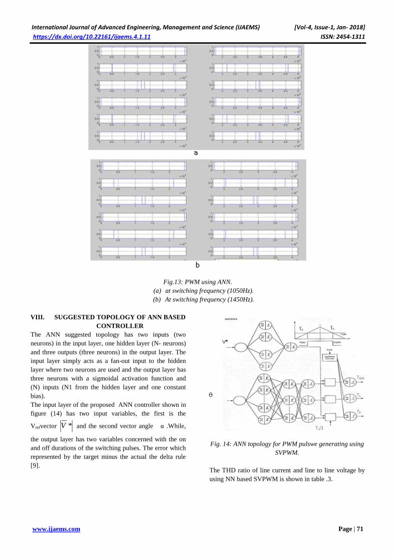
International Journal of Advanced Engineering, Management and Science (IJAEMS) [Vol-4, Issue-1, Jan- 2018]
1311-ISSN: 2454 https://dx.doi.org/10.22161/ijaems.4.1.11
71| Page www.ijaems.com
Fig.13: PWM using ANN.
(a) at switching frequency (1050Hz).
(b) At switching frequency (1450Hz).
VIII. SUGGESTED TOPOLOGY OF ANN BASED
CONTROLLER
The ANN suggested topology has two inputs (two
neurons) in the input layer, one hidden layer (N- neurons)
and three outputs (three neurons) in the output layer. The
input layer simply acts as a fan-out input to the hidden
layer where two neurons are used and the output layer has
three neurons with a sigmoidal activation function and
(N) inputs (N1 from the hidden layer and one constant
bias).
The input layer of the proposed ANN controller shown in
figure (14) has two input variables, the first is the
Vrefvector *V and the second vector angle α .While,
the output layer has two variables concerned with the on
and off durations of the switching pulses. The error which
represented by the target minus the actual the delta rule
[9].
Fig. 14: ANN topology for PWM pulswe generating using
SVPWM.
The THD ratio of line current and line to line voltage by
using NN based SVPWM is shown in table .3.

International Journal of Advanced Engineering, Management and Science (IJAEMS) [Vol-4, Issue-1, Jan- 2018]
1311-ISSN: 2454 https://dx.doi.org/10.22161/ijaems.4.1.11
72| Page www.ijaems.com
Table.3: THD ratio of line current and line to line voltage
by NN based SVPWM.
Switching
frequency(Hz)
Line current
THD value(%)
Line -line Voltage THD
value(%)
1050 4.308 % 0.4535 %
1450 2.744 % 0.4535 %
Figure. 15 represents the circuit diagram of VSI-HVDC
using ANN based SVPWM.
Fig.15: Block diagram represents SVPWM based on ANN
with Inverter bridge.
The THD ratio of the line current for switching
frequencies1050Hz and 1450Hz after applying NN is
shown in figure. 16.
Fig.16: THD ratio of line current in time domain after
applying NN based SVPWM.
(a) at switching frequency (1050Hz).
(b) at switching frequency (1450Hz).
The THD ratio of the line to line voltage for 1050Hz and
1450Hz switching frequencies after applying NN is
shown in figure. 17.
Fig.17: THD ratio of line to line voltage in time domain
after applying NN based SVPWM.
(a) at switching frequency (1050Hz).
(b) at switching frequency (1450Hz).
IX. CONCLUSION
When using the NN controller based SVPWM the THD
value of line current and line to line voltage is improved
as a percentage ratio by 74.65% and 78.28% respectively
as compared with SVPWM at switching frequency
1050Hz, and these value are improved as a percentage
ratio by 68.1% and 65.72% respectively as compared with
SVPWM and switching frequency 1450Hz.
At switching frequency 1450Hz the THD ratio is reduced
as compared with the switching frequency 1050Hz but the
filter losses are increased.
REFERENCES
[1] Vijay, K. Sood "HVDC and FACTS Controllers"
Kluwer power electronics and power editions series,
2004.
[2] Michael, P., Johnson, B., and B " the ABC of HVDC
Transmission Technologies" , power and energy
magazine, 5, March/Aplil 2007.
[3] Padiyar, K.R., Prabhu, N., " Modeling Control
Design and Analysis of VSC Based HVDC
Transmission" Paper published in POWERCOM
2004, 21-24 November, Singapore.
[4] Guangkai, Li., et al " Research on Dynamic
Characteristics of VSC-HVDC System " power
Engineering Society General Meeting , IEEE, 2006.
[5] Song, R., et al. " VSCs Based HVDC and its Control
Strategy" Electric Power Research Institute, Beijing,
China, IEEE/PES Transmission and Distribution
Conference 2005.
[6] Vironis, T. D., et al " Optimal Integration Fan
Offshore Wind Farm to a Weak AC Grid" IEEE
Transactions on Power delivery , 21,2, April 2006.

International Journal of Advanced Engineering, Management and Science (IJAEMS) [Vol-4, Issue-1, Jan- 2018]
1311-ISSN: 2454 https://dx.doi.org/10.22161/ijaems.4.1.11
73| Page www.ijaems.com
[7] Subrata, K.,Joao,O.P.,Bimal, K.,"A Neural-
Network-Based Space-Vector PWM Controller for a
Three-Level Voltage-Fed Inverter Induction Motor
Drive" IEEE Transactions on Industry Applications,
38,3,PP:660-669, 2002.
[8] Vassilios, G.,A., Georgios, D., D., Nikolas, F., "
Recent Advances in High-Voltage Direct-Current
Power Transmission Systems",
[9] Van, H. W., Skudelny, H.C., Stank, G., " Analysis
and Realization of a Pulse Width Modulator Based
on Voltage Space Vectors" IEEE Transactions
Industry Applications Application, 24, 1,pp:1530-
1535, 1998.
[10] Bakhshai,A., Joos, G., Esinoza, J., "Fst Space Vector
Moulation Based on a Neurocomuting Digital Signal
Processor", in Proc. APEC'97,pp: 872-878, 1997.
[11] Amitava D., Debasish L and Barnali K" Space
Vector PWM Based AC Output Voltage Contrrol of
Z- Source Inverter" IEEE Transactions on Industry
Applications, January 2, 2010.
[12] "PulseWidthModulation(PWM)Technique"www2.e
ce.ohiostate.edu/ems/PowerConverter/lect25.ppt
[13] Abdul Hamid B. and PramodA."An Artificial-
Neural – Network- Based Space Vector PWM of a
Three-Phase High Power Factor Converter for
Power Quality Improvement" IEEE Transactions on
Industry Applications, January 2, 2010.
[14] L. Fausett, "Fundamental of Neural Networks,
Architectures, Algorithms and applications", Printice
Hall Int. Snc., 1994.

International Journal of Advanced Engineering, Management and Science (IJAEMS) [Vol-4, Issue-1, Jan- 2018]
https://dx.doi.org/10.22161/ijaems.4.1.12 ISSN: 2454-1311
www.ijaems.com Page | 74
Quantic Analysis of Formation of a Biomaterial
of Latex, Retinol, and Chitosan for Biomedical
Applications Karina García-Aguilar1, 2, Iliana Herrera-Cantú1, Erick Pedraza-Gress1, Lillhian Arely
Flores-Gonzalez1, Manuel Aparicio-Razo 1, 4, Oscar Sánchez-Parada3, Emmanuel
Vázquez-López1, Juan Jesús García-Mar1 and Manuel González-Pérez1, 5
1Universidad Popular Autónoma del Estado de Puebla A.C. (UPAEP).
Centro Interdisciplinario De Posgrados (CIP). Posgrado en Ciencias de la Ingeniería Biomédica. 2Instituto Tecnológico Superior de Coatzacoalcos. Académica de Ingeniería Bioquímica
3Escuela de Medicina Universidad Popular Autónoma del Estado de Puebla 4Benemérita Universidad Autónoma de Puebla, Facultad de Ciencias de la Electrónica
5Sistema Nacional De Investigadores. Nivel 1.
Abstract— The present work shows the quantum
theoretical analysis and practical tests for the formation
of a homogeneous mixture with Latex (Lx), Chitosan (Qn)
and Retinol (Rl), which work as possible biomaterial for
regeneration of epithelial tissue. Lx, Qn, and Rl
compounds molecules were designed through Hyperchem
to get the coefficient of electrostatic potential
calculations. The amounts used to create the biomaterial
are minimum depending on the quantities of molecules
used in chemical design. A positive calculation was
obtained for the reaction of these three compounds and
the formation of the biomaterial in physical checking
theory etc.
Keywords— Quantum analysis, Latex, Chitosan,
Retinol, Biomaterial.
I. INTRODUCTION
Latex Lx is a colloidal aqueous suspension composed of
fats, waxes and gummy resins, white and milky in
appearance. Rubber (CA) is a hydrocarbon that is
suspended in the Lx of trees in tropical and subtropical
areas. [1] The CA or rubber is inside the Lx and presents
a chemical formula c5H8. The chemical composition of
the Lx has oils, sugars, mineral salts, proteins, terpenes,
nucleic acids, hydrocarbons, waxes, resins, starch, tannins
and balms. It has a neutral pH (7-7.2). Passed between
twelve and twenty-four hours since removal, pH drops to
5.0, came the coagulation of the substance when it is
located with a pH equal to or less than 4.2. [2]
It is characterized for being a substance insoluble in
water, electric and elastic resistance. Most of the Lx is
commercial use is extracted from the Syrinx (Hevea
brasiliensis) and is dedicated to the production of rubber.
The Lx prevents the entry of pathogenic micro-organisms
and promotes the healing process when there is a wound.
Allergen Lx Hev 2 b with properties β-1, 3-glucanase
accelerate the hydrolytic scission of polymers β-1, 3
glucans, basic component of the cell wall of fungi. This
protein can prevent fungal infections to the plant through
the degradation of the cell wall of fungal pathogens. The
allergen in latex Hev b 11 endoquitinasa activity and
could participate in the hydrolytic scission of chitin.
Another protein that plays a role in defense is the
hevamina. Acts by catalyzing the scission of the links β-1,
4-glucosidic linkages of chitin and the peptidoglycans of
cell surface. [3]
Studies with Lx only explain their function with patients
who have diabetic ulcers. The idea was to implement a
template for a biomaterial (Lx) for the control of the
pressure of the diabetic foot. [4]
Chitosan (QN) is a polysaccharide that is naturally in the
cell walls of some fungi. The main source of production
is between alkaline chitin hydrolysis. The presence of
groups amines in the polymer chain has made one of the
most versatile materials Chitosan by the possibility to
perform a wide variety of modifications such as reactions
the anchor of enzymes for applications in biomedicine.
[5]
(RN) retinol or vitamin A is fat-soluble and necessary is
biological processes such as the formation and
maintenance of epithelial cells. This vitamin is retinol, the
retinal and Retinoic acid. Formed from provitamin beta
carotene and other Pro-vitamins in the tract of the large
intestine. It is stored in the liver.
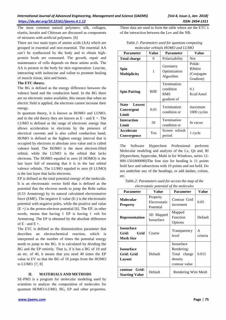
International Journal of Advanced Engineering, Management and Science (IJAEMS) [Vol-4, Issue-1, Jan- 2018]
https://dx.doi.org/10.22161/ijaems.4.1.12 ISSN: 2454-1311
www.ijaems.com Page | 75
The most common natural polymers: silk, collagen,
elastin, keratin and Chitosan are discussed as components
of mixtures with artificial polymers. [6]
There are two main types of amino acids (AA) which are
grouped in essential and non-essential. The essential AA
can’t be synthesized by the body and to obtain high-
protein foods are consumed. The growth, repair and
maintenance of cells depends on these amino acids. The
AA is present in the body for skin regeneration: Leucine,
interacting with isoleucine and valine to promote healing
of muscle tissue, skin and bones.
The ETC theory.
The BG is defined as the energy difference between the
valence band and the conduction band. In the BG there
are no electronic states available; this means that when an
electric field is applied, the electrons cannot increase their
energy.
In quantum theory, it is known as HOMO and LUMO,
and in the old theory they are known as E - and E +. The
LUMO is defined as the range of electronic energy that
allows acceleration in electrons by the presence of
electrical currents and is also called conduction band;
HOMO is defined as the highest energy interval that is
occupied by electrons in absolute zero value and is called
valence band. The HOMO is the most electron-filled
orbital, while the LUMO is the orbital that lacks
electrons. The HOMO equaled to zero (0 HOMO) is the
last layer full of meaning that it is in the last orbital
valence orbitals. The LUMO equaled to zero (0 LUMO)
is the last layer that lacks electrons.
EP is defined as the total potential energy of the molecule.
It is an electrostatic vector field that is defined as the
potential that the electron needs to jump the Bohr radius
(0.53 Armstrong) by its natural calculated electromotive
force (EMF). The negative E value (E-) is the electrostatic
potential with negative poles, while the positive and value
(E +) is the proton-electron potential [6]. The EP, in other
words, means that having 1 EP is having 1 volt for
Armstrong. The EP is obtained by the absolute difference
of E - and E +.
The ETC is defined as the dimensionless parameter that
describes an electrochemical reaction, which is
interpreted as the number of times the potential energy
needs to jump to the BG. It is calculated by dividing the
BG and the EP entirely. That is, if it has a BG of 10 and
an etc. of 40, it means that you need 40 times the EP
value in EV so that the BG of 10 jumps from the HOMO
to LUMO. [7, 8]
II. MATERIALS AND METHODS
SE-PM3 is a program for molecular modeling used by
scientists to analyze the composition of molecules for
quantum HOMO-LUMO, BG, EP and other properties.
These data are used to form the table where are the ETC´s
of the interaction between the Lev and the NB.
Table.1: Parameters used for quantum computing
molecular orbitals HOMO and LUMO
Parameter Value Parameter Value
Total charge 0 Polarizability Not
Spin
Multiplicity 1
Geometry
Optimization
Algorithm
Polak-
Ribière
(Conjugate
Gradient)
Spin Pairing RHF
Termination
condition
RMS
gradient of
0.1
Kcal/Amol
State Lowest
Convergent
Limit
0.01 Termination
condition or
maximum
1000 cycles
Interaction
Limit 50
Termination
condition or In vacuo
Accelerate
Convergence Yes
Screen refresh
period 1 cycle
The Software Hyperchem Professional performs
Molecular modeling and analysis of the Lx, Qn and, Rl
(Hyperchem, hypercube, Multi in for Windows, series 12-
800-1501800080)The font size for heading is 11 points
bold face and subsections with 10 points and not bold. Do
not underline any of the headings, or add dashes, colons,
etc.
Table.2: Parameters used for access the map of the
electrostatic potential of the molecules
Parameter Value Parameter Value
Molecular
Property
Property
Electrostatic
Potential
Contour Grid
increment 0.05
Representation 3D Mapped
Isosurface
Mapped
Function
Options
Default
Isosurface
Grid: Grid
Mesh Size
Coarse Transparency
level
A
criteria
Isosurface
Grid: Grid
Layout
Default
Isosurface
Rendering:
Total charge
density
contour value
0.015
contour Grid:
Starting Value Default Rendering Wire Mesh
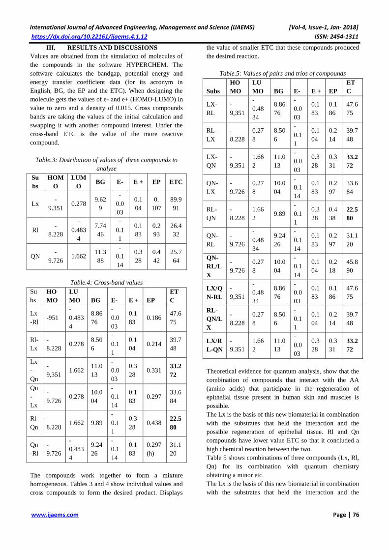
International Journal of Advanced Engineering, Management and Science (IJAEMS) [Vol-4, Issue-1, Jan- 2018]
https://dx.doi.org/10.22161/ijaems.4.1.12 ISSN: 2454-1311
www.ijaems.com Page | 76
III. RESULTS AND DISCUSSIONS
Values are obtained from the simulation of molecules of
the compounds in the software HYPERCHEM. The
software calculates the bandgap, potential energy and
energy transfer coefficient data (for its acronym in
English, BG, the EP and the ETC). When designing the
molecule gets the values of e- and e+ (HOMO-LUMO) in
value to zero and a density of 0.015. Cross compounds
bands are taking the values of the initial calculation and
swapping it with another compound interest. Under the
cross-band ETC is the value of the more reactive
compound.
Table.3: Distribution of values of three compounds to
analyze
Su
bs
HOM
O
LUM
O BG E- E + EP ETC
Lx -
9.351 0.278
9.62
9
-
0.0
03
0.1
04
0.
107
89.9
91
Rl -
8.228
-
0.483
4
7.74
46
-
0.1
1
0.1
83
0.2
93
26.4
32
QN -
9.726 1.662
11.3
88
-
0.1
14
0.3
28
0.4
42
25.7
64
Table.4: Cross-band values
Su
bs
HO
MO
LU
MO BG E- E + EP
ET
C
Lx
-Rl -951
-
0.483
4
8.86
76
-
0.0
03
0.1
83 0.186
47.6
75
Rl-
Lx
-
8.228 0.278
8.50
6
-
0.1
1
0.1
04 0.214
39.7
48
Lx
-
Qn
-
9,351 1.662
11.0
13
-
0.0
03
0.3
28 0.331
33.2
72
Qn
-
Lx
-
9.726 0.278
10.0
04
-
0.1
14
0.1
83 0.297
33.6
84
Rl-
Qn
-
8.228 1.662 9.89
-
0.1
1
0.3
28 0.438
22.5
80
Qn
-Rl
-
9.726
-
0.483
4
9.24
26
-
0.1
14
0.1
83
0.297
(h)
31.1
20
The compounds work together to form a mixture
homogeneous. Tables 3 and 4 show individual values and
cross compounds to form the desired product. Displays
the value of smaller ETC that these compounds produced
the desired reaction.
Table.5: Values of pairs and trios of compounds
Subs
HO
MO
LU
MO BG E- E + EP
ET
C
LX-
RL
-
9,351
-
0.48
34
8.86
76
-
0.0
03
0.1
83
0.1
86
47.6
75
RL-
LX
-
8.228
0.27
8
8.50
6
-
0.1
1
0.1
04
0.2
14
39.7
48
LX-
QN
-
9,351
1.66
2
11.0
13
-
0.0
03
0.3
28
0.3
31
33.2
72
QN-
LX
-
9.726
0.27
8
10.0
04
-
0.1
14
0.1
83
0.2
97
33.6
84
RL-
QN
-
8.228
1.66
2 9.89
-
0.1
1
0.3
28
0.4
38
22.5
80
QN-
RL
-
9.726
-
0.48
34
9.24
26
-
0.1
14
0.1
83
0.2
97
31.1
20
QN-
RL/L
X
-
9.726
0.27
8
10.0
04
-
0.1
14
0.1
04
0.2
18
45.8
90
LX/Q
N-RL
-
9,351
-
0.48
34
8.86
76
-
0.0
03
0.1
83
0.1
86
47.6
75
RL-
QN/L
X
-
8.228
0.27
8
8.50
6
-
0.1
1
0.1
04
0.2
14
39.7
48
LX/R
L-QN
-
9.351
1.66
2
11.0
13
-
0.0
03
0.3
28
0.3
31
33.2
72
Theoretical evidence for quantum analysis, show that the
combination of compounds that interact with the AA
(amino acids) that participate in the regeneration of
epithelial tissue present in human skin and muscles is
possible.
The Lx is the basis of this new biomaterial in combination
with the substrates that held the interaction and the
possible regeneration of epithelial tissue. Rl and Qn
compounds have lower value ETC so that it concluded a
high chemical reaction between the two.
Table 5 shows combinations of three compounds (Lx, Rl,
Qn) for its combination with quantum chemistry
obtaining a minor etc.
The Lx is the basis of this new biomaterial in combination
with the substrates that held the interaction and the

International Journal of Advanced Engineering, Management and Science (IJAEMS) [Vol-4, Issue-1, Jan- 2018]
https://dx.doi.org/10.22161/ijaems.4.1.12 ISSN: 2454-1311
www.ijaems.com Page | 77
possible regeneration of epithelial tissue. Rl and Qn
compounds have lower value ETC so that it concluded a
high chemical reaction between the two.
Table.6: Interaction of reducing and oxidizing component
of Lx and Rl
Reduc
er
Oxidiz
er
Interacti
on ETC
Limi
ts
Pure
Substan
ces
LX LX LX - Lx
89.9
90 Top
RL RL RL - Rl
26.4
32
Low
er
Cross
band
LX RL LX - Rl
41.6
31
RL LX RL - Lx
39.5
62
Graphs of quantum well (figures 1) have two lines that
represent the upper and lower limits (greater ETC). Black
dots plotted are the percentage of probability of occurring
a chemical reaction with the combination of two of the
three compounds.
Fig.1: Quantum well, Lx-Rl ETC interaction
Tables 6 and 7 show interactions between reducing and
oxidizing compounds for the upper and lower limits and
graphing quantum wells etc.
Table.7: Interaction of the component reducing and
oxidizing of Lx and Qn
Reduc
er
Oxidiz
er
Interacti
on ETC
Limi
ts
Pure
Substan
ces
LX LX LX - Lx
89.9
9 Top
Qn Qn Qn - Qn
26.4
32
Low
er
Cross
band
LX Qn LX - Qn
33.2
71
Qn LX Qn - Lx
33.6
83
Figure 1 shows an average probability of interaction
between the two compounds (50% probability). Figure 2
shows the same probability of interaction.
Fig.2: Quantum well, the interaction between Lx and Qn
ETC
Fig.3: Emptying of Lx, Qn and Rl for field testing on lab
in the formation of a new biomaterial
In Figure 3 are observed practices carried out in the
laboratory to check the quantum theoretical calculated
previously.
Fig.4: Form of Biomaterial with Lx, Qn, and Rl
Figure 4 shows laboratory tests proving that quantum
calculation (calculation of high chemical reaction
between compounds) ETC is the biomaterial.
Table 8 shows the interactions of mixtures of the
biomaterial the AA main compounds necessary for the
regeneration of epithelial and muscle tissue. Minor
interactions are likely chemical reaction between the
mixtures working as oxidants and antioxidants. Obtaining
ETC describes that the reaction will be likely to benefit
from the growth of epithelial cells in patients who have
superficial wounds.

International Journal of Advanced Engineering, Management and Science (IJAEMS) [Vol-4, Issue-1, Jan- 2018]
https://dx.doi.org/10.22161/ijaems.4.1.12 ISSN: 2454-1311
www.ijaems.com Page | 78
Table.8: Pairs of AA with mixtures of Lx, Qn, and Rl
N
o
Red
ucer
Oxi
dize
r
HO
MO
LU
MO
B
G
E
-
E
+
E
P
E
T
C
1
QN-
RL/
LX
LEU
-
GLY
-
9.73
0.9
0
10.
63
-
0.
1
1
0.
1
6
0.
2
7
38
.9
2
QN-
RL/
LX
LEU
-
LYS
-
9.73
0.9
4
10.
67
-
0.
1
1
0.
1
9
0.
3
1
34
.5
3
LEU
-
LYS
QN-
RL/
LX
-
9.64
0.2
7
9.9
2
-
0.
1
3
0.
1
0
0.
2
3
43
.1
4
QN-
RL/
LX
ILE-
GLN
-
9.73
0.7
5
10.
48
-
0.
1
1
0.
1
9
0.
3
1
34
.2
5
QN-
RL/
LX
ILE-
LYS
-
9.73
0.9
4
10.
67
-
0.
1
1
0.
1
9
0.
3
1
34
.5
6
QN-
RL/
LX
GLY
-ILE
-
9.73
0.9
7
10.
70
-
0.
1
1
0.
1
9
0.
3
0
35
.4
7
QN-
RL/
LX
GLY
-
GLN
-
9.73
0.7
5
10.
48
-
0.
1
1
0.
1
9
0.
3
1
34
.2
8
QN-
RL/
LX
LYS
-ILE
-
9.73
0.9
7
10.
70
-
0.
1
1
0.
1
9
0.
3
0
35
.4
9
QN-
RL/
LX
VAL
-
GLN
-
9.73
0.7
5
10.
48
-
0.
1
1
0.
1
9
0.
3
1
34
.2
1
0
QN-
RL/
LX
VAL
-ILE
-
9.73
0.9
7
10.
70
-
0.
1
1
0.
1
9
0.
3
0
35
.4
1
1
QN-
RL/
LX
VAL
-
LYS
-
9.73
0.9
4
10.
67
-
0.
1
1
0.
1
9
0.
3
1
34
.5
1
2
LEU
-
GL
N
LX/
RL-
QN
-
9.64
1.6
6
11.
31
-
0.
1
3
0.
3
3
0.
4
5
24
.9
1
3
LEU
-
GL
Y
LX/
RL-
QN
-
9.64
1.6
6
11.
31
-
0.
1
3
0.
3
3
0.
4
5
24
.9
1
4
LEU
-
LYS
LX/
RL-
QN
-
9.64
1.6
6
11.
31
-
0.
1
3
0.
3
3
0.
4
5
24
.9
1
5
ILE-
LYS
LX/
RL-
QN
-
9.87
1.6
6
11.
53
-
0.
1
3
0.
3
3
0.
4
5
25
.1
1
6
GL
Y-
ILE
LX/
RL-
QN
-
9.90
1.6
6
11.
56
-
0.
1
4
0.
3
3
0.
4
6
24
.9
1
7
LYS
-
GL
Y
LX/
RL-
QN
-
9.52
1.6
6
11.
18
-
0.
1
3
0.
3
3
0.
4
5
24
.6
1
8
VA
L-
GL
N
LX/
RL-
QN
-
9.91
1.6
6
11.
58
-
0.
1
3
0.
3
3
0.
4
6
25
.2
IV. CONCLUSION
1. The Lx is highly reaccionable with compounds Qn
and Rl.
2. The combination of the three compounds (Lx, Qn,
Rl) is possible by low levels that present etc.
3. The highest interaction is with the Qn and Rl when
working as antioxidant and oxidant respectively.
4. By combining three compounds is calculated an etc.
of 33.2719033 when the Lx works as a reducing
agent.
5. The compounds shown in its quantum wells High
solubility and formation of striation.
6. Experiments prove the quantum chemistry
calculations.
7. Forms a patch of Lx, Qn, and Rl.
8. The ETC child occur with Rl-Qn 22.57.
9. Lx, Qn, and Rl compounds interact with the AA of
epithelial and muscle tissue.
10. The combination of the three main compounds for
the biomaterial have high reaction with the AA.
REFERENCES
[1] Narciso, A. R. M. (1974). The exploitation of rubber
in Mexico and its use in the world.
[2] Carreon Blaine, Emilie a. (2006). The olli in the
plastic Aztec: the use of rubber in the 16th century.
UNAM. ISBN 970-32-2200-5.

International Journal of Advanced Engineering, Management and Science (IJAEMS) [Vol-4, Issue-1, Jan- 2018]
https://dx.doi.org/10.22161/ijaems.4.1.12 ISSN: 2454-1311
www.ijaems.com Page | 79
[3] Fireman, Philip. Atlas of Allergy and Immunology
clinic. Elsevier Mosby. p-261.
[4] Rosa, S. D. S. R. F., do Carmo Reis, M., Rosa, M. F.
F., Colon, D., dos Reis, C. A., & Balthazar, J. M.
(2015). Use of Natural Latex as a Biomaterial for the
Treatment of Diabetic Foot-A New Approach to
Treating Symptoms of Diabetes Mellitus. In Topics
in Public Health. InTech.
[5] Velasquez, C. (2003). Some applications of chitosan
in aqueous systems. Revista Iberoamericana of
polymers, 4 (2), 91.
[6] Sionkowska, a. (2011). Current research on the
blends of natural and synthetic polymers as new
biomaterials. Progress in Polymer Science, 36 (9):
1254-1276.
[7] Mondragon-jimenez, jesus francisco, et al. interaction
of methylenedioxymethamphetamine vs.
neurotransmitters and the relationship by the
quantum method. 2017
[8] Gonzalez-perez, m. chemical-quantum analysis of the
aggressiveness of glucose and its appeasement with
atp inside the cell and water as an excellent
antioxidant, 2017.
[9] Firmin H. Aikpo, Miriac Dimitri S. Ahouanse,
Lucien Agbandji, Patrick A. Edorh, Christophe S.
Houssou(2017).Assessment of contamination of soil
by pesticides in Djidja's cotton area in Benin.
International Journal of Advanced Engineering
Research and Science (ISSN : 2349-6495(P) | 2456-
1908(O)),4(7), 001-005.
http://dx.doi.org/10.22161/ijaers.4.7.1
[10] Perfect, T. J., & Schwartz, B. L. (Eds.) (2002).
Applied metacognition Retrieved from
http://www.questia.com/read/107598848
[11] Myers, D. G. (2007). Psychology(1stCanadian ed.).
New York, NY: Worth.
[12] Cognition.(2008). In Oxford reference online
premium dictionary. Retrieved from
http://www.oxfordreference.com
[13] Blue, L. (2008, March 12).Is our happiness
preordained? [Online exclusive]. Time. Retrieved
from http://www.time.com/time/health
[14] J. Clerk Maxwell, A Treatise on Electricity and
Magnetism, 3rd ed., vol. 2. Oxford: Clarendon, 1892,
pp.68–73.
[15] I. S. Jacobs and C. P. Bean, “Fine particles, thin films
and exchange anisotropy,” in Magnetism, vol. III, G.
T. Rado and H. Suhl, Eds. New York: Academic,
1963, pp. 271–350.
[16] K. Elissa, “Title of paper if known,” unpublished.
[17] R. Nicole, “Title of paper with only first word
capitalized,” J. Name Stand. Abbrev., in press.