Edinburgh Research Explorer

Experimental and numerical studies characterizing the burningdynamics of wildland fuels

Citation for published version:El houssami, M, Thomas, JC, Lamorlette, A, Morvan, D, Chaos, M, Hadden, R & Simeoni, A 2016,'Experimental and numerical studies characterizing the burning dynamics of wildland fuels' Combustion andflame, vol 168, pp. 113-126. DOI: 10.1016/j.combustflame.2016.04.004

Digital Object Identifier (DOI):10.1016/j.combustflame.2016.04.004

Link:Link to publication record in Edinburgh Research Explorer

Document Version:Peer reviewed version

Published In:Combustion and flame

General rightsCopyright for the publications made accessible via the Edinburgh Research Explorer is retained by the author(s)and / or other copyright owners and it is a condition of accessing these publications that users recognise andabide by the legal requirements associated with these rights.

Take down policyThe University of Edinburgh has made every reasonable effort to ensure that Edinburgh Research Explorercontent complies with UK legislation. If you believe that the public display of this file breaches copyright pleasecontact openaccess@ed.ac.uk providing details, and we will remove access to the work immediately andinvestigate your claim.

Download date: 27. Jun. 2018

1

Experimental and Numerical Studies Characterizing the Burning Dynamics of Wildland Fuels M. El Houssami1*, J.C. Thomas1, A. Lamorlette2, D. Morvan2, M. Chaos3, R. Hadden1, A. Simeoni4 *Corresponding author: M.elhoussami@ed.ac.uk 1BRE Centre for Fire Safety Engineering, The University of Edinburgh, Edinburgh, EH9 3JL, UK 2Aix-Marseille Université, CNRS, Centrale Marseille, M2P2 UMR 7340, 13451 Marseille, France 3FM Global, Research Division, 1151 Boston-Providence Turnpike, Norwood, MA 02062, USA 4Exponent, Inc, 9 Strathmore Road, Natick, MA 01760, USA

Abstract A method to accurately understand the processes controlling the burning behavior of porous wildland fuels is presented using numerical simulations and laboratory experiments. A multiphase approach has been implemented in OpenFOAM, which is based on the FireFOAM solver for large eddy simulations (LES). Conservation equations are averaged in a control volume containing a gas and a solid phase. Drying, pyrolysis, and char oxidation are described by interaction between the two phases. Numerical simulations are compared to laboratory experiments carried out with porous pine needle beds in the FM Global Fire Propagation Apparatus (FPA). These experiments are used to support the use and the development of submodels that represent heat transfer, pyrolysis, gas-phase combustion, and smoldering processes. The model is tested for different bulk densities, two distinct species and two different radiative heat fluxes used to heat up the samples. It has been possible to reproduce mass loss rates, heat release rates, and temperatures that agree with experimental observations, and to highlight the current limitations of the model. Nomenclature

a Thermal diffusivity R Ideal gas constant c Speed of light Re Reynolds number C, C’ Convective heat transfer constants s Stoichiometric O2/C mass ratio CEDC, Cdiff EDC model coefficients T, Ts Gas and solid phase

temperatures Cp Specific heat capacity Tr Radiation source temperature D Epyr, Echar, Evap

Equivalent diameter Energy activation for pyrolysis,

Y"#$(&) , Y)*+

(&) Mass fraction of dry pine needle and water in solid phase

charring and vaporization YF, YO2 Fuel and oxygen mass fraction Gr Grashof number Greek symbols hp Planck’s constant αeff Effective absorptivity I Spectral intensity αflam Effective absorptivity from

flame J Irradiance αchar Char absorptivity K Air thermal conductivity βchar Char correction factor Kpyr, Kchar, Kvap Pre-exponential factors for pyrolysis,

charring and vaporization Δ LES filter size

kb Boltzmann constant Δhchar Δhpyr Δhvap

Reaction heat for charring, pyrolysis and vaporization

kSGS Sub grid scale kinetic energy εSGS Sub grid scale dissipation rate m, m’ Convective heat transfer coefficient

constants λ Wavelength

n, n’ Convective heat transfer coefficient constants

ρ ρs

Gas density Fuel (solid phase) density

Nu Nusselt number σ σs

Stefan–Boltzmann constant Surface to volume ratio (SVR)

2

Pr Prandtl number ϕg, ϕs Volume fraction of gas, solid phase

Q-+./0 ,Q#1"

0 Convective and radiation heat transfer source terms

χ Convective heat transfer coefficient

q34155 , q&67855 Imposed and corrected heat fluxes ω3555, ω-)1#555 ,

ω4$#555 , ω/14555 Volumetric rate of gas combustion, pyrolysis, charring, and vaporization

q;<=55 Net energy received by the solid fuel

1. Introduction Many experimental studies on wildland fuel flammability are conducted at small bench scale or even at microscopic scale, such as Thermogravimetric Analysis (TGA) [1, 2] and Differential Scanning Calorimetry (DSC) [3–5] to understand the physical and chemical processes involved during the decomposition of the fuel when heated [2, 6]. While it is difficult to perform large scale experiments, to maintain repeatable and fully controlled environments [7–9], and to monitor all the dynamics involved, the use of numerical models becomes essential. Different types of models exist and they are used to predict wildfires. They are either based on empirical correlations [10–13], simplified models [14, 15], or detailed computational fluid dynamics (CFD) models [16–18]. These CFD models are often used to study large fires [18–21], in which many parameters and complex submodels are included in order to provide satisfactory results.

The first aim of this study is to perform experiments at an intermediate scale that is small enough to maintain a controlled environment, and large enough to be comparable to real fire conditions. Therefore, experiments are conducted in the FM-Global fire propagation apparatus (FPA) [22, 23], which allows repeatable conditions to be achieved, and to monitor temperature, heat release rate (HRR), gas production and mass loss rates (MLR) as in [24–26]. In tests performed for the present work, temperature was measured inside the fuel bed to make sure that the heat transfer (radiation and convection) is modeled correctly during the heating phase, before ignition, where there is no flame radiation and soot oxidation yet. Measurements of gas production allow determining the HRR, which indicates how the energy is released. Finally, mass loss indicates the degradation rate, including evaporation, pyrolysis and char oxidation. Mass loss is also linked to the burning rate, which, along with the surrounding conditions, will affect the HRR, flame height and the burning rate. Separately, spectral measurements have been done for dead pine needles under a wide spectrum (0.25 – 20 µm) to determine the effective absorptivity of the fuel under the FPA halogen lamps, used to heat up the samples.

Numerical simulations are then conducted to mimic the same experimental conditions to verify how well the model behaves and to understand its limitations. The numerical approach is based on the multiphase model [17, 27–29] that was implemented in OpenFOAM [30] and called ForestFireFOAM. The latter is built following the structure of FireFOAM, a LES code for fire modeling [31]. The multiphase formulation is used to include the process of degradation of the forest fuel by drying, pyrolysis and heterogeneous combustion, and to simulate it by assuming a volumetric reaction rate. This approach was not yet implemented neither in OpenFOAM, nor in FireFOAM. Consequently, part of this study has been dedicated to the implementation of this new model. The multiphase approach was introduced by Grishin [27], in which he presented an extensive review of the work conducted in USSR in the 1970s and 1980s on wildland fires. Grishin’s model was the first to incorporate kinetics to describe pyrolysis, combustion, and hydrodynamics through a fuel bed using a multiphase approach. Thermal equilibrium was initially assumed between gas phase and solid phase and the equations were averaged over the height of the forest canopy to simplify the formulation. Later, Larini et al. [28] presented the bases of the multiphase formulation for a medium in which a gas phase and N solid phases in thermal non-equilibrium are treated individually along with some one-dimensional applications. A detailed review of these models are presented in [32].

3

The multiphase model includes the Navier-Stokes conservation equations [33] for radiative and reactive multiphase medium. The closure models, or submodels that are used for degradation, heat transfer, combustion, and radiation are typically applied to simulate large-scale wildfires in complex environments. However, they were obtained from micro- and small- scale laboratory experiments using very different conditions than the ones where they are often applied in the literature [20, 27, 28, 34, 35]. These submodels are described and examined hereafter at intermediate scale. The multiphase model is tested with experiments using fuel beds with different bulk densities that are representative of litter conditions. Two distinct North American species with different surface to volume ratios are burnt at two different heat fluxes imposed by the FPA heaters. Pine needle beds are used as a reference fuel because they are well characterized in the literature [36] and they allow obtaining repeatable fuel bed properties under laboratory settings. Moreover, pine needle beds often accumulate on forest floor and near structures in the Wildland Urban Interface (WUI), increasing the fire risk [37].

2. Experimental configuration

2.1. FPA experiments Experiments were performed with the FM Global Fire Propagation Apparatus (FPA), which provides controlled and repeatable conditions [24, 26] (Fig. 1), such as the ability to produce a constant incident radiative heat flux. No forced flow was applied in this study, only natural convection was allowed through the porous samples. As the lower end of the FPA is closed, natural convection is limited at the backface of the sample. Dead needles were packed in cylindrical open baskets of 12.6 cm diameter and 3.0 cm depth following the protocol used in [38]. MLR was derived from mass loss measurements using a sensitive scale (± 0.01g) and the exhaust gases were analyzed for composition. HRR was calculated by Oxygen Consumption (OC) calorimetry [24, 39] and vertical temperature was measured inside the porous bed, at the surface and at different depths, using fine K-type thermocouples (0.127 mm diameter). It is impossible to ensure that all thermocouples are in contact with a pine needle at all time. Therefore, separate tests were performed to quantify the influence of a touching needle on a thermocouple. The difference was very negligible at all time (<4˚C).

Figure 1: Overview of the Fire Propagation Apparatus (FPA)

Experiments were carried out for dead pitch (Pinus rigida) and white pine (Pinus strobus) needles under two different heat fluxes, 20 and 50 kW/m2. Pine needles were scooped off the ground, and collected in paper

4

bags. Care was given to only take the top layer of the litter and not include the duff layer. After collection, needles were dried in ambient air and were stored in dry conditions to prevent further degradation. Fuel moisture content (FMC) was determined by conditioning needles at 60°C for 24 hours. The average FMC was approximately 7% of the dry weight. The FPA heaters were kept on during the entire experiment, mimicking a strong flame feedback from a larger fire surrounding the sample. Pitch and white pines have different surface to volume ratios (SVR). The fuel properties are listed in Table 1. The specific heat capacity (cp) is averaged (between ambient and 200˚C) from DSC analysis that were specifically performed for this study. Four different bulk densities are tested: 17, 23, 30 and 40 kg/m3 corresponding to a sample mass of 6.4 g, 8.7 g, 11.4 g, and 15 g, respectively. More details of the experimental setup are provided in [26]. The bulk density (ρb) is calculated from the sample mass over the sample holder volume. The porosity (ϕg) is then calculated as: ϕ? = 1 − CD

CE (1)

Where ρs is the pine needle density (Table 1). In separate experiments, a Fourier Transform Infra-Red Spectrometer (FTIR) [40] was used to analyze pyrolysis gases for pitch pine before ignition. It was mounted at 50 cm above the sample using the same protocol in the FPA.

Table 1: Summary of species properties Species Pitch pine

(Pinus rigida) White pine

(Pinus strobus) Density [kg/m3] 607 621

SVR [m-1] 7295 14173 Cp [J/kg K] 2069.7 2090.4

FMC 0.07 0.07 Diameter [mm] 1.39 0.50

2.2. Spectral measurements Forest fuel emissivity/absorptivity is highly spectrally dependent [41]. Indeed, it was observed that FPA heaters operate in a very specific spectrum band [41–43]. Reference [43] indicates that for PMMA and wood samples, the absorptivity is relatively high in the operating wavelengths range of the conical heater but relatively low for the range of the tungsten lamps. Therefore, the spectral reflectivity of dead pitch pine needles was measured over a wide range of wavelengths, from ultraviolet to long infrared (0.25-20 µm) at FM Global laboratory. This range is similar to those of [44, 45] and much broader than those considered in other literature studies concerned with the spectral characteristics of vegetation [46, 47]. However, it is necessary to ensure that the fraction of blackbody (or greybody) emissive power contained within the spectral band is as high as possible for temperatures typical of fires and bench-scale tests, such as those conducted in the FPA. This range covers the spectral radiance spectrum of the FPA infrared heaters, which are very dominant in the near infrared. The material and methodology applied are the same as in [45]. With known reflectivity, the emissivity (absorptivity) of the samples is determined by invoking Kirchhoff’s law of thermal radiation [48, 49]. This approach assumes a completely opaque surface. Indeed, the transmissivity of the prepared pine needle samples was measured and it was found to be negligible (< 0.5%) over the wavelength range considered. This means that the samples were sufficiently thick to be optically opaque. The FPA heaters can be considered to be greybody radiators and their corresponding spectral intensity I (kW/m2/µm/sr) can be represented using Planck’s equation [45].

I λ, T = I×KL*MNOP*

QRexp KLVNOP

QWXY− 1

ZK (2)

5

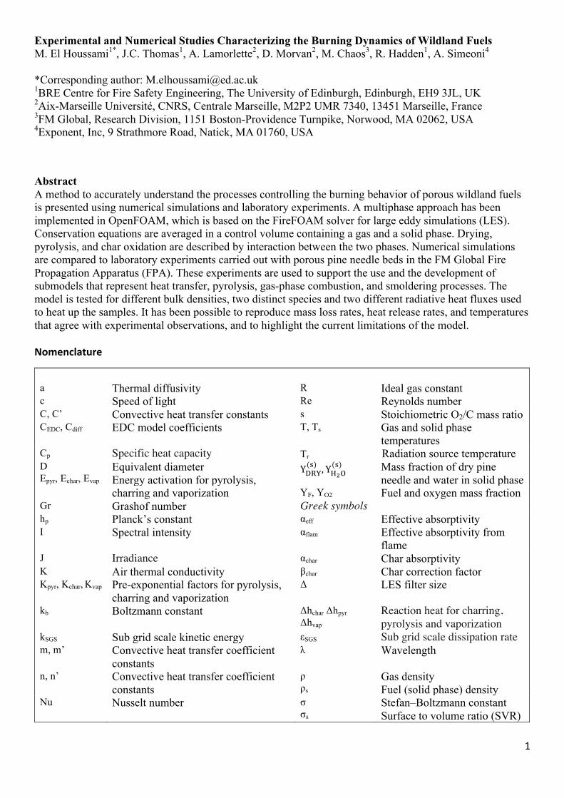
Where λ is the wavelength (µm), hp is Planck’s constant, c is the speed of light, kB is Boltzmann’s constant, and T is a given temperature (K). The spectral radiative intensity curve is normalized and plotted along with the pine needle spectral absorptivity in Fig. 2. Highly non-grey spectral distributions are evident for the pine needle absorptivity. The standard deviation of the six measurements taken for each of the needles is also represented in Fig. 2. There is noted variability (approximately 40%), especially in the near infrared region (~1-3 µm, 3300-10000 cm-1), which indicates that the needles are not perfectly diffuse reflectors and directional effects are present. The present data are also in good agreement with those of Acem et al. [47] for Aleppo pine (Pinus halepensis) needles, and those of Clark et al. [50] for lodgepole pine (Pinus contorta) needles.

Figure 2: Spectral emissivity/absorptivity of dead pitch pine needle, and FPA heaters at 2140 K and at

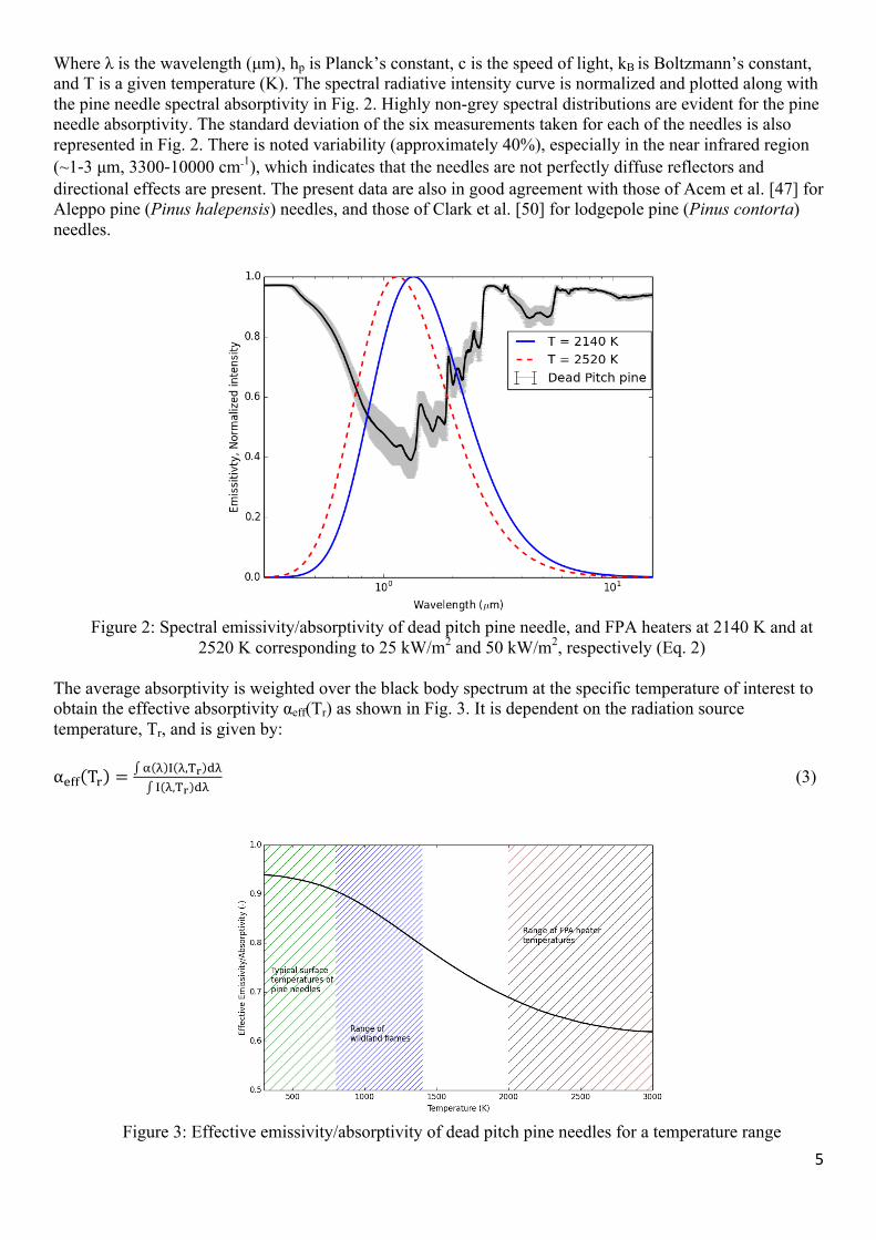
2520 K corresponding to 25 kW/m2 and 50 kW/m2, respectively (Eq. 2) The average absorptivity is weighted over the black body spectrum at the specific temperature of interest to obtain the effective absorptivity αeff(Tr) as shown in Fig. 3. It is dependent on the radiation source temperature, Tr, and is given by: α<88 T7 = \ Q ] Q,Y^ _Q

] Q,Y^ _Q (3)

Figure 3: Effective emissivity/absorptivity of dead pitch pine needles for a temperature range

6

As mentioned above, dead needles are highly non-grey absorbers/emitters and differ most notably in the near- and mid-infrared spectral regions. This behavior has direct implications on the radiative source term in the energy balance equation and the radiative transfer equation (RTE) [33], which require that the spectral radiation environment interacting with the needles be taken into account. For example, the pine needles considered in the present study would absorb radiation more efficiently from low temperature sources (characterized by longer wavelengths) than from those at higher temperatures. On the other hand, emission of radiation (i.e., re-radiation) from the pine needles would be determined by their surface temperature, which may considerably differ from those of the radiation sources interacting with them. Therefore, one needs to determine the effective emissivity and absorptivity of the pine needles as a function of temperature. Figure 3 shows the evolution of αeff with temperature. The FPA heaters radiate at temperatures of 2000 K < Tr < 3000 K [45] where the effective absorptivity of dead needles differs by approximately 10 to 15% (on average, αeff = 0.64 for dead needles, over this temperature range). On the other hand, typical surface temperatures are characterized by 300 K < T < 1000 K for which the effective emissivity of dead needles (αeff = 0.92 on average) differs by about 3%. Naturally, needles start charring around 573 K [51]; however, char spectrally behaves like a greybody with effective emissivity and absorptivity equal to 0.85 [44, 45].

3. Numerical Model:

3.1. Multiphase approach The interactions between solid fuel constituting of a forest fuel layer and the gas phase are represented by adopting a multiphase formulation [27, 28, 33]. The general formulation of the multiphase approach is particularly relevant to forest fuels and our small scale fires of pine needle beds. The following assumptions are made for simplicity: - The fuel bed is considered as a homogeneous distribution of solid particles whose dimensions and

physical properties are evaluated from experimental data. - Solid particles are motionless and fixed in space. - Contact between particles is neglected. - Fuel particles are considered thermally thin, meaning that the temperature throughout any solid particle

is uniform at all times. This approach consists in solving conservation equations (mass, momentum, and energy) averaged in a control volume at an adequate scale that contains a gas phase flowing through a solid phase and considering the strong coupling between both phases [27]. Here, only one solid phase is considered, and consists of particles of the same geometrical and thermophysical properties. The required formulation is made of Navier-Stokes radiative and reactive equations with interface relationships to represent solid and gas phase coupling [33]. The fuel properties must be characterized using physical variables such as fuel density (ρs), SVR (σs), fuel moisture content (FMC), solid temperature (Ts), specific heat capacity (CP), and fuel volume fraction (φS).

3.2. Submodels Physico-chemical processes such as pyrolysis, evaporation, and char oxidation occurring in the solid and gas phases are considered as well as other phenomena including combustion, radiative and convective heat transfer [52]. These submodels are used to close the balance equations, and are described hereafter. They are often obtained from small-scale experiments under various conditions and have not been fully validated for the multiphase approach [53]. Some limitations and improvements are detailed later in the discussion. In this situation heat transfer is only considered through radiation and convection, since conduction is neglected

7

due to the poor conductivity of pine needles. Indeed, the contact area between adjacent pine needles is very small due to the geometrical configuration in pine litters, as with the high porosity (93-97%).

3.2.1. Radiation The source term corresponding to the radiative heat transfer 𝑄abc

(d) in the energy equation [33] is written as follows: 𝑄abc(d) = efgf

h𝛼jkk 𝐽 − 4𝜎𝑇ph (4)

with efgf

hrepresenting the solid fuel extinction coefficient for spherical particles [14], J is the irradiance, and

σ is Stefan-Boltzmann constant (5.67 x 10-8 m-2K-4). It was shown in [41] that value of the extinction coefficient can be used with a small correction factor varying from 0.95 to 0.99. The radiative heat transfer equation is solved for a number of finite solid angles using a discrete ordinate method (fvDOM) [54] available in OpenFOAM [30]. Representing the radiative heat transfer is a key factor in fire scenarios, especially in environments such as the FPA. In order to simulate the experiments performed in the FPA correctly, it was important to estimate the effective absorptivity of the vegetation under the FPA lamps as described earlier. Typical flame temperatures observed in ventilated conditions usually are much cooler that the operating FPA heater temperatures, hence they are better absorbed and the corresponding effective absorptivity is 0.85 < αflam < 0.95, which is much higher than what is found for the FPA heaters (~0.64). In consequence, pine needles absorb the flame radiation more than the heater radiation. Instead of numerically separating the incoming flame radiation and the FPA heater radiation, and treating both radiations separately, the fuel absorptivity 𝛼jkk in equation (4) was set as αflam. Whereas the imposed heat flux on the surface of the fuel is corrected using the effective absorptivity of pine needles under the FPA heaters, as found in the spectral analysis: 𝑞prsk55 = 𝛼jkk𝑞tub55 (5) This simulates that the heaters only emit the fraction that can be absorbed. This simplification allowed both radiation sources to be treated the same way in the solid phase. Cellulosic materials have similar spectral distributions [41, 45, 47], and dead pine needle behavior is comparable to those of hardwood, and oak [45]. Differences can be mostly attributed to moisture content in the samples as well as color differences for shorter wavelengths (i.e., larger wavenumbers). Given these observations, we can safely assume that the spectral emissivity of pine needle char is very similar to that of other cellulosic materials. Curves of charred materials do not exhibit the strong spectral variations shown by the virgin materials [45]; therefore, these chars are approximated as gray emitters with flat spectral profiles with an average emissivity value αchar = 0.85 [45]. Most of char production becomes apparent once the fuel starts burning. Hence, αeff increases linearly with the produced char fraction until reaching αchar. As for the flame radiation, it is primarily due to the presence of CO2 and H2O in the gas phase and to the oxidation of soot particles in the flame. A soot model is added to evaluate the volume fraction of soot produced and oxidized. It is originally based on Syed’s model [55] and was tested for CH4/air diffusion flames by Kaplan et al. [56]. The multiphase adaptation of the model is presented in [17], where soot formation is accounted for a percentage (3%) of pyrolysis products. The sensitivity of the soot model, and the influence of the flame feedback on the sample are assumed to be acceptable since these flames are not considered very sooty.

3.2.2. Convection Generally, convection could play an important role in heat transfer. In the current setup with only natural convection, the influence of convection is not dominant, but can be higher on top of the sample than inside

8

the sample, because of its exposure to the induced air that can either cool down or heat up the solid phase. The term representing the contribution due to convective heat transfer 𝑄vwxy

(d) between gases and the unburned solid fuel is written as follows in the energy balance equation [33]: 𝑄vwxy(d) = ϕp𝜎pχ(𝑇 − 𝑇p) (6)

With T and Ts the gas and solid phase temperatures, respectively. The heat transfer coefficient χ can be estimated using Hilpert correlation [52] for low Reynolds numbers: Nu = }"

~= C𝑅𝑒�𝑃𝑟� (7)

K is the air thermal conductivity (in W/m.K) and D the equivalent diameter approximated as 4/σs. Since samples are prepared by stacking pine needles over each other, one can assume that the heat transfer coefficient is similar to the one for array of staggered cylinders in cross flow. Many correlations are given to represent the Nusselt (Nu) number in these specific or similar conditions [52, 57, 58] that are widely applied in studies using the multiphase approach [20, 33, 59] even under natural convection [35, 60]. However, an over estimation of the heat transfer coefficient in the FPA configuration with no forced inflow prevents the solid temperature from rising enough to ignite and to maintain a steady flame. Since the setup is made under natural convection, it is more appropriate to use correlations depending on the Grashof number. This leads to smaller heat convective coefficients, such as: χ = ~

cC′(GrPr)�5 (8)

Where C′=0.119, n′=0.3 [57] resulting in χ < 20 W/m2K typically for Gr < 10; the difference between using correlations based on either Re or Gr are non negligible and have direct effect on the degradation rate and the burning in this configuration. After a qualitative analysis on the possible values of the heat transfer coefficient, any constant value of 10 < χ < 20 W/m2K are suitable in this configuration and has negligible influence on the process.

3.2.3. Degradation Under the action of the intense heat flux coming from the FPA heaters and from the flaming zone, the decomposition of the fuel can be summarized using the three following steps: evaporation, pyrolysis and smoldering. Evaporation rate 𝜔ybu555 is represented using a one-step first-order Arrhenius kinetics law whose parameters (frequency factors and activation energy) are evaluated from TGA analysis [17, 27]. Hence, it is important to verify how well it behaves when coupled with other phenomena. This rate is highly dependent on the solid phase temperature.

𝜔ybu555 = ϕp𝜌p𝑌�*w(p) 𝑇ZK/I𝐾ybu𝑒

�������f (9)

Pyrolysis rate is represented using a using a two-step first-order Arrhenius kinetics law with the first step defined as in [6, 17, 27]. This simplistic model should be bounded by the net heat flux received (𝑞�j�55 ) once high temperatures are reached in the solid phase. A similar approach is used in [20, 61]. It limits the reaction because it does not only depend on the kinetics anymore, but on the flux received. One of the main problems using only a 1st order Arrhenius correlation is that the kinetics are not the only involved phenomena, as in TGA environment (by design), in fact the initiation step of preheating is strongly related to the geometrical properties of the samples (thickness, size of leaves and branches) [62]. Moreover, it is not detailed enough to represent the degradation model accurately. Thus, the following 2-step model was used:

9

𝜔u�a555 =ϕp𝜌p𝑌ca�

(p) 𝐾u�a𝑒�������f , 𝑇p ≤ 800𝐾

 ¡¢£¤¤

¥¦§¨© , 𝑇p > 800𝐾

(10)

The limiting temperature was found in order to best match experimental data for both pine species and for different heat fluxes and different bulk densities. Pyrolysis gases were analyzed using a FTIR device sampling above the combustion chamber in the FPA at low heat flux (10kW/m2). Such low heat flux was used to avoid ignition and to capture pyrolysis gases only. Pyrolysis gas products are mainly composed of CO, CO2, CH4, and of lower amounts of C2, and C4 hydrocarbons (Table 2). These results are comparable to what was found for Pinus halepensis, Pinus larcio and Erica arborea with mass spectrometers in [63]. No C3 hydrocarbons were found in this analysis and H2O measurement has been excluded due to the FTIR limitations [64]. It is assumed that the combustible part of the pyrolysis products can be assimilated to a mixing of 65% of CO and 35% of partially oxidized hydrocarbons (CHO) that includes CH4, C2Hx and C4Hy . Using the same approach as in [21], the combustion of the pyrolysis products in the gas phase can be written as follows using a single step reaction: 𝐶𝐻𝑂L.¯° +

²³hL𝑂I → 𝐶𝑂I +

KI𝐻I𝑂 (11)

Table 2: Mass fractions of the main pyrolysis gases released by degradation of pitch pine before ignition

Gas Mass fraction CO 0.199 CO2 0.687 CH4 0.026 C2Hx 0.027 C4Hy 0.061

Char oxidation, or smoldering rate represents the incomplete combustion that produces CO, which burns in the gas phase. 𝐶(p) + K

I𝑂I(µ) → 𝐶𝑂(µ) (12)

It is represented using a one-step Arrhenius equation multiplied by a corrective factor that is a function of the Reynolds number. This accounts for blowing effects [59], which forces the charring reaction (𝜔v�ba555 ) in no flow condition, because a simple Arrhenius equation is not sufficient to maintain the reaction.

𝜔v�ba555 = efgf¶·*

ϕµ𝜌𝑌w*𝐾v�ba𝑒��¸¹����f 1 + 𝛽v�ba 𝑅𝑒 (13)

The fraction of energy produced by the char combustion contributes is equally split between the gas and the solid phase. This assumption is widely used in different studies [20, 27, 28, 33, 35] but has never been validated experimentally. Other parameters in the energy equation are sensitive to this value. For instance, if the fraction is higher for the solid phase than for the gas phase, then more energy is kept in the solid phase (increasing Ts), and less energy is released to the gas phase (reducing T). In consequence, 𝑄vwxy

(d) (Eq. 6) is expected to increase, whereas 𝑄abc

(d) should decrease. However, it is very difficult to quantify experimentally the heat flux from the solid alone (excluding gas radiation), and to separate the radiative and the convective heat flux. This is why the assumption that the fraction of energy is equally split between the gas and solid phase was not changed in this study.

10

3.2.4. Turbulence and combustion The turbulent sub-grid scale stress is modeled by the eddy viscosity concept through a one-equation model for the turbulent kinetic energy K [65], with an additional sink term due to dissipation of sub-grid-scale energy [33]. Instead of using an Eddy Dissipation Concept (EDC) for turbulent combustion [66], an extension of the same model is applied, where the characteristic time scale of fuel-air mixing is different under turbulent and laminar flow conditions [67]. This model is more appropriate since the flame has a laminar base and is turbulent in the intermittent zone due to external influences (air movement) [68]. The gas rate of combustion is expressed as: 𝜔t555 =

»

¼½; ¾¿À¿¸�Á¸Â¿À¿

, Ã*¸ÁÄÅÅÆ

min 𝑌t,�·*p

(14)

𝑌t and 𝑌w* are the fuel and oxygen mass fraction, Δ is the LES filter size, a is the thermal diffusivity, 𝐶Écv =

4 and 𝐶cÊtt= 10. The ratio Ë¿À¿Ì¿À¿

is the turbulent time scale and the ratio ¥*

Íis the molecular diffusion time

scale. The pilot flame was not simulated because in this model flaming combustion will always occur if fuel and oxidizer are mixed, regardless of the available amount of energy to activate the combustion. In this study, time to ignition is overlooked, since it is known that it depends on the distance between the pilot flame and the sample. To allow the sample to heat up without having early local ignitions, and to allow the pyrolysis gases to accumulate before igniting, a Lower Flammability Limit (LFL) [68] condition was used. This condition also allows obtaining similar ignition times than the ones found experimentally [26], but this effect is beyond the scope of this study.

3.3. Numerical configuration The set of transport equations in the gas phase are solved using a second order implicit Finite Volume method. Total Variation Diminishing (TVD) schemes have been adopted to avoid introduction of false numerical diffusion [69]. The set of Ordinary Differential Equations governing the evolution of the solid fuel was solved using a second order explicit method. Adaptive time step is calculated based on Courant-Fredrichs-Lewy (CFL) number [69], with a maximum value of 0.7 to achieve temporal accuracy and numerical stability. In this study, only two-dimensional calculations are performed. BlockMesh and snappyHexMesh [30] mesh generators supplied with OpenFOAM are used to create robust meshes. The overall domain is a rectangle of 5 m wide and 2 m high. The mesh was composed primarily of hexahedral cells. Based on a mesh sensitivity study, a mesh resolution of (0.001 m)2 was determined as providing converging results in the vicinity of the sample and near the lamps. The mesh is stretched above the lamps and beyond the zone of interest until the boundaries, in order to reduce computational time. The side boundaries are open allowing entrainment of air. However, the ground and combustion chamber have a wall boundary condition applied for velocity and a Dirichlet condition for temperature. An outlet boundary condition is set at the top above the flame, representing the exhaust hood. The entrained air from the open boundaries is at 293 K. The domain geometry is presented in Fig. 4. Lamps were modeled by fixing a constant heat flux on specified walls. These have the same view factor as in the FPA, giving the same heat flux required on the sample surface. A sensitivity study was carried out to determine an adequate amount of discretization for the radiative heat transfer equation. 256 solid angles were found optimal providing a uniformly distributed radiative heat flux at the top of the fuel sample, as observed in the FPA.

11

Figure 4: Computational domain (not to scale)

4. Results & Discussion During the heating process from the start of the test until ignition only heat transfer plays an essential role in the temperature evolution, since there is neither combustion nor flame involved yet. Since no forced flow was applied (𝑄vwxy

(d) is small), and if we neglect change of properties (dehydration), we can assume that the gas and the fuel are in thermal equilibrium before ignition. Fig. 5 and 6 show the numerical predictions and experimental results for the temperature evolution in depth, at different positions in the sample (from the surface to the back face). Simulated temperatures are the same for solid and gas. They display a good agreement with the measured temperature in the fuel bed. Only solid phase temperatures are shown for the sake of clarity. The overall prediction is satisfactory with 31˚C maximum deviation from experimental results. The model captures well the trends observed from the experimental data at 25 kW/m2 and at 50 kW/m2. There is a 5 to 10 s delay between experimental and numerical ignition times. Even if these ignition times are not exactly the same, it is verified that temperatures at ignition time are matching for both heat fluxes.

Figure 5: Temperature profile before ignition for pitch pine, bulk density of 40 kg/m3, 25 kW/m2 applied

heat flux. Symbols: Experiments, lines: Simulation

12

Figure 6: Temperature profile before ignition for pitch pine, bulk density of 40 kg/m3, 50 kW/m2 applied

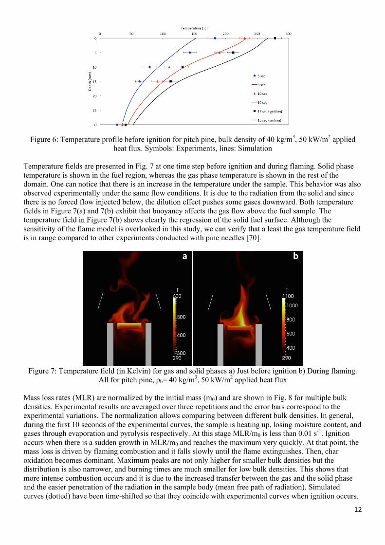
heat flux. Symbols: Experiments, lines: Simulation Temperature fields are presented in Fig. 7 at one time step before ignition and during flaming. Solid phase temperature is shown in the fuel region, whereas the gas phase temperature is shown in the rest of the domain. One can notice that there is an increase in the temperature under the sample. This behavior was also observed experimentally under the same flow conditions. It is due to the radiation from the solid and since there is no forced flow injected below, the dilution effect pushes some gases downward. Both temperature fields in Figure 7(a) and 7(b) exhibit that buoyancy affects the gas flow above the fuel sample. The temperature field in Figure 7(b) shows clearly the regression of the solid fuel surface. Although the sensitivity of the flame model is overlooked in this study, we can verify that a least the gas temperature field is in range compared to other experiments conducted with pine needles [70].

Figure 7: Temperature field (in Kelvin) for gas and solid phases a) Just before ignition b) During flaming.

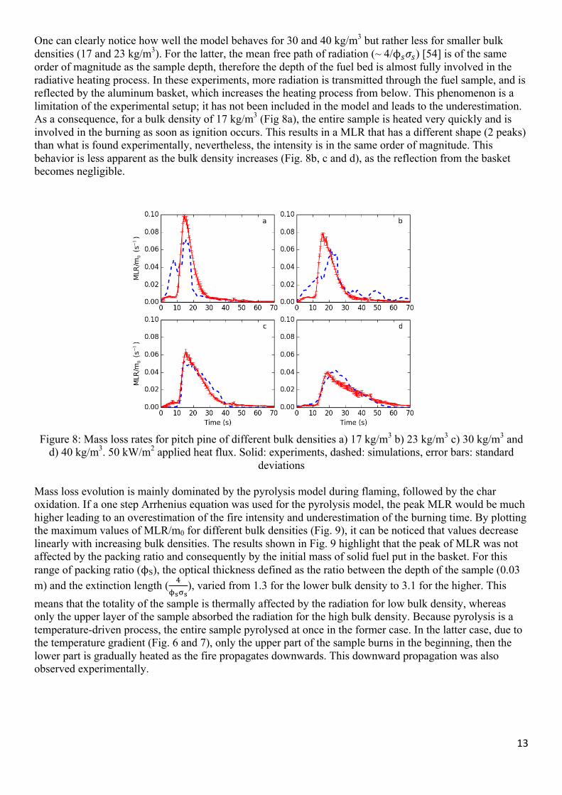
All for pitch pine, ρb= 40 kg/m3, 50 kW/m2 applied heat flux Mass loss rates (MLR) are normalized by the initial mass (m0) and are shown in Fig. 8 for multiple bulk densities. Experimental results are averaged over three repetitions and the error bars correspond to the experimental variations. The normalization allows comparing between different bulk densities. In general, during the first 10 seconds of the experimental curves, the sample is heating up, losing moisture content, and gases through evaporation and pyrolysis respectively. At this stage MLR/m0 is less than 0.01 s-1. Ignition occurs when there is a sudden growth in MLR/m0 and reaches the maximum very quickly. At that point, the mass loss is driven by flaming combustion and it falls slowly until the flame extinguishes. Then, char oxidation becomes dominant. Maximum peaks are not only higher for smaller bulk densities but the distribution is also narrower, and burning times are much smaller for low bulk densities. This shows that more intense combustion occurs and it is due to the increased transfer between the gas and the solid phase and the easier penetration of the radiation in the sample body (mean free path of radiation). Simulated curves (dotted) have been time-shifted so that they coincide with experimental curves when ignition occurs.

13

One can clearly notice how well the model behaves for 30 and 40 kg/m3 but rather less for smaller bulk densities (17 and 23 kg/m3). For the latter, the mean free path of radiation (~ 4/ϕp𝜎p) [54] is of the same order of magnitude as the sample depth, therefore the depth of the fuel bed is almost fully involved in the radiative heating process. In these experiments, more radiation is transmitted through the fuel sample, and is reflected by the aluminum basket, which increases the heating process from below. This phenomenon is a limitation of the experimental setup; it has not been included in the model and leads to the underestimation. As a consequence, for a bulk density of 17 kg/m3 (Fig 8a), the entire sample is heated very quickly and is involved in the burning as soon as ignition occurs. This results in a MLR that has a different shape (2 peaks) than what is found experimentally, nevertheless, the intensity is in the same order of magnitude. This behavior is less apparent as the bulk density increases (Fig. 8b, c and d), as the reflection from the basket becomes negligible.

Figure 8: Mass loss rates for pitch pine of different bulk densities a) 17 kg/m3 b) 23 kg/m3 c) 30 kg/m3 and

d) 40 kg/m3. 50 kW/m2 applied heat flux. Solid: experiments, dashed: simulations, error bars: standard deviations

Mass loss evolution is mainly dominated by the pyrolysis model during flaming, followed by the char oxidation. If a one step Arrhenius equation was used for the pyrolysis model, the peak MLR would be much higher leading to an overestimation of the fire intensity and underestimation of the burning time. By plotting the maximum values of MLR/m0 for different bulk densities (Fig. 9), it can be noticed that values decrease linearly with increasing bulk densities. The results shown in Fig. 9 highlight that the peak of MLR was not affected by the packing ratio and consequently by the initial mass of solid fuel put in the basket. For this range of packing ratio (ϕS), the optical thickness defined as the ratio between the depth of the sample (0.03 m) and the extinction length ( h

eEÎE), varied from 1.3 for the lower bulk density to 3.1 for the higher. This

means that the totality of the sample is thermally affected by the radiation for low bulk density, whereas only the upper layer of the sample absorbed the radiation for the high bulk density. Because pyrolysis is a temperature-driven process, the entire sample pyrolysed at once in the former case. In the latter case, due to the temperature gradient (Fig. 6 and 7), only the upper part of the sample burns in the beginning, then the lower part is gradually heated as the fire propagates downwards. This downward propagation was also observed experimentally.

14

Figure 9: Measured maximum values of mass loss rates and normalized mass loss rates for pitch pine at 50kW/m2 for different bulk densities and their corresponding trendlines. Error bars: standard deviations

This result is confirmed by looking at the evolution of the ratio MLR/m0 that follows exactly the evolution of the initial solid fuel mass m0. When it is not normalized (red), these peaks are rather constant for the bulk densities tested. Indeed, they increase very slowly, keeping a linear trend with increasing bulk densities. This means that the intensities are similar regardless of the bulk densities tested. Only the burning duration increases with bulk density, as it is presented in Fig. 10, where the corresponding heat release rates (HRR) are plotted. Similarly to the MLR behavior, the HRR is averaged for three repetitions. The uncertainty/variability of the experimental measurements is illustrated by the error bars added to the mean values. HRR was determined by oxygen consumption (OC) calorimetry as described in [24]. As with the numerical MLR, acceptable predictions only occur for higher bulk densities. The peak HRR increases with the bulk density experimentally and in the model. It can also be noticed that the peaks are wider as the bulk density increases, meaning that the burning times including flaming and smoldering become longer. For a small amount of solid fuel (17 and 23 kg/m3) the quantity of combustible gases released during pyrolysis could affect the conditions of ignition and sustainability of the flame and consequently the HRR, via the amount of gaseous fuel effectively burned and the retroaction (by radiation of soot particles) of the flame toward the solid fuel. From the green dotted lines, representing flame out times, one can observe that smoldering (post flameout) times increase with the bulk densities. This is due to the geometrical or the “packing effect” that limits fresh air from reaching the fuel, hence slows down the smoldering combustion. In consequence it also increases the total burning time with the bulk density. The HRR after flameout is underestimated for most cases (Fig. 10). It is because the rate of the char oxidation was underestimated. In fact, the char oxidation rate was not maintained after flame out as the temperature was dropping. In result, the total heat released is smaller than it should be. Therefore, a single step model is not enough to represent this complex phenomenon in the tested conditions. The peak HRR at 40 kg/m3 (Fig. 10d) is at approximately 8 kW, which is comparable to what was found in Schemel et al. [24] for Aleppo pine (Pinus halepensis) tested in the same condition. Tests were also performed at 25 kw/m2 for pitch pine needles to evaluate the model’s accuracy at low heat flux (Fig. 11). Lower bulk densities have been tested and show very similar results once ignition occurs, both experimentally and numerically. In Fig. 11, one can notice experimental MLR is slightly higher for higher heat fluxes (Fig. 8d) during smoldering (after 40 s) that could be due to the external heat flux sustaining the oxidation of the char. Concerning the numerical predictions, they are in agreement with the experiments: the main tendencies are found, except for the end of the curve (after 40 s), where char oxidation drops again. Ignition times are different but it is not shown in this study for clarity. By evaluating the radiative Biot number defined as:

𝐵Ða =Ñ¢ÒÒ fÓ©Ò

¤¤

Ôfgf¥Õ (15)

15

With λs= 0.12 W/mK being the fuel conductivity, ΔT= 300 K, and αeff = 0.64. BiR= 0.06 for q&678'' = 25

kW/m2; whereas, BiR = 0.12 for q&678'' = 50 kW/m2. Hence, it is not always below the limit of the thermally

thin hypothesis BiR < 0.1 [71, 72]. Nevertheless, numerical results show good agreement with experiments,

which means that the temperature gradient inside a needle is not large enough conflict with the thermally thin assumption. For the same reason, the temperature is better matched for lower heat flux (in Fig. 5) than for higher heat flux (Fig. 6) The radiative Biot number is smaller for the lower heat fluxes. Hence, the thermally thin assumption is more effective.

Figure 10: Heat release rates of pitch pine for different bulk densities: a) 17 kg/m3 b) 23 kg/m3 c) 30 kg/m3 and d) 40 kg/m3. 50 kW/m2 applied heat flux. Solid: experiments, dashed: simulation, green vertical dotted

lines: flame out

Figure 11: Normalized mass loss rates of pitch pine at 25 kW/m2, bulk density of 40 kg/m3. Solid:

experiments, dashed: simulations

16

The same tests were conducted on white pine needles providing MLR and HRR shown in Fig. 12 and 13, respectively. Computed curves have been time-shifted so that they coincide with experimental curves when ignition occurs (17 s). The time shift was always between 5 to 15 s, but it was not consistent between different simulations and experiments, therefore time to ignition is not successfully predicted. This is not surprising because piloted ignition is such a marginal event that any small variation in the experiment or in the numerical condition can influence it. Additionally, the experimental uncertainty for ignition is very high [26]. In Fig. 12, during the first 17 s of the simulation, a higher amount of mass is lost resulting in an increase in the HRR that is not observed experimentally (Fig. 13). This is because the HRR was measured by OC and there was not sufficient Oxygen consumed before ignition to discern that step. Then, when ignition occurred, the slope of MLR and HRR are much steeper numerically than experimentally, due to the available fuel that was pyrolysed previously. The other two humps around 30 and 40 s correspond to a combination of the smoldering reaction taking over and the fire (heat wave) reaching the bottom boundary of the sample. Despite all that, the peak HRR and peak MLR show good agreement. However, burning times are underestimated again because of the char oxidation, resulting in less total heat released. Pitch pine beds are less compact than those of white pine, due to the geometrical properties of the specie (SVR). It induces bigger gaps inside the bed, allowing oxygen to pass through more efficiently. Hence, pitch pine releases more energy than white pine during flaming (Fig. 10d and Fig. 13). These results are in agreement with the experiments conducted in [73] with different pine species. Burning time of pitch pine is longer than for white pine. This agrees with Anderson’s observation [74] on the statement that residence time in a fire spread increases with particle thickness. Computed MLR for white pine show better agreement with experimental data than for pitch pine, except for the energy released by char oxidation again. The overall agreement can be explained by the fact that white pine needles are finer than pitch pine needles; white pine needles are characterized by a Surface to Volume ratio (SVR) two times larger than for pitch pine needles (Table 1). Even for a relatively high heat flux (50 kW/m2), the Biot number is less than one (similar to pitch pine with 25 kW/m2) which is compatible to a thermally thin assumption. Thus, the transition from thermally thin to thermally thick is more likely to occur for pitch pine than for white pine.

Figure 12: Normalized mass loss rate for white pine at 50 kW/m2, bulk density of 40 kg/m3. Solid:

experiments, dashed: simulation

17

Figure 13: Heat release rate for white pine at 50 kW/m2, bulk density of 40 kg/m3. Solid: experiments,

dashed: simulation 5. Conclusion An experimental and numerical study on the burning dynamics of wildland fuels was presented. The FPA was used to obtain a controlled environment and repeatable conditions to burn litters of pine needles. Additional experiments were done in order to understand and to describe with mathematical formulations all the different aspects involved in these experiments, such as analyzing the spectral emissivity of dead pine needles to better describe the radiative heat transfer. The effective absorptivity of pine needles is lower under the FPA heaters radiation (0.64) than when submitted to flame radiation (~0.8). Pyrolysis gases were analyzed using a FTIR to better represent the gas phase combustion, and similar mass fractions were found as for other wildland fuels. The use of a multiphase approach was implemented to OpenFOAM, creating ForestFireFOAM solver for porous fuels. Multiple submodels of this formulation were tested: An appropriate pyrolysis model was found to mimic the experimental conditions with no forced flow and giving quantitatively similar MLR and HRR for high bulk densities only (30 and 40 kg/m3). Findings are comparable for lower bulk densities (17 and 23 kg/m3) in terms of order of magnitude, but different behaviors are found due to the easier penetration of the radiation in the sample body that increases the heating rate. It was not attempted to adapt the model because it is only a limitation of the experimental setup and does not reflect the applicability of the multiphase model. It was shown that underestimating the contribution of the char oxidation leads to underestimating MLR and HRR. In fact, the char oxidation rate was not sustained after flame out. Therefore, a single step model does not represent this complex phenomenon efficiently in natural convection. We deliberately chose to show that one-step models for char oxidation are not appropriate. Indeed, the use of this model is often assumed to be correct without further justifications [20, 29, 53, 75, 76]. In consequence, burning times and zones can be misjudged when simulating larger fires. An extended EDC gas phase combustion model was used in this study; it has the advantage to consider laminar flow characteristics instead of only turbulent flows. As for the convection model, it was found that the convective heat transfer coefficient is overestimated when standard correlations depending on the Reynolds value are used for litters in natural convection. Instead, a constant value that can be estimated from the Grashof number should be used. By varying the bulk density, the heat fluxes and the species, we were able to determine which submodels can be used in the tested conditions, and which ones cannot be applied. The model performs well for higher heat fluxes (50 kW/m2) and for high bulk densities (30 - 40 kg/m3), but is still very sensible to each submodel. Soot modeling and flame radiation were overlooked in this study; it will be the object of a future study.

18

Acknowledgment The authors gratefully acknowledge Drs Y. Wang, K. Meredith, P. Chatterje, A. Gupta, and N. Ren for the numerous discussions and help provided in the development of ForestFireFOAM. The reviewers are also acknowledged for their useful analysis, which has significantly improved the article. This work was granted access to the HPC resources of Aix-Marseille Université financed by the project Equip@Meso (ANR-10-EQPX-29-01) of the program « Investissements d’Avenir » supervised by the Agence Nationale pour la Recherche. References 1. Font R, Conesa JA, Moltó J, Muñoz M (2009) Kinetics of Pyrolysis and Combustion of Pine Needles

and Cones. Journal of Analytical and Applied Pyrolysis 85:276–286. doi: 10.1016/j.jaap.2008.11.015

2. Leroy V, Cancellieri D, Leoni E, Rossi JL (2010) Kinetic Study of Forest Fuels by TGA: Model-Free Kinetic Approach for the Prediction of Phenomena. Thermochimica Acta 497:1–6.

3. Leoni E, Cancellieri D, Balbi N, Tomi P, Bernardini AF (2003) Thermal Degradation of Pinus Pinaster Needles by DSC , Part 2 : Kinetics of Exothermic Phenomena. doi: 10.1177/073490402032834

4. Cancellieri D, Leoni E, Rossi JL (2005) Kinetics of the thermal Degradation of Erica Arborea by DSC: Hybrid Kinetic Method. Thermochimica Acta 438:41–50.

5. Leroy V, Cancellieri D, Leoni E (2006) Thermal Degradation of Ligno-Cellulosic Fuels: DSC and TGA Studies. Thermochimica Acta 451:131–138. doi: 10.1016/j.tca.2006.09.017

6. Di Blasi C, Branca C, Santoro A, Gonzalez Hernandez E (2001) Pyrolytic Behavior and Products of Some Wood Varieties. Combustion and Flame 124:165–177. doi: 10.1016/S0010-2180(00)00191-7

7. Santoni PA, Simeoni A, Rossi JL, Bosseur F, Morandini F, Silvani X, Balbi JH, Cancellieri D, Rossi L (2006) Instrumentation of Wildland Fire: Characterisation of a Fire Spreading Through a Mediterranean Shrub. Fire Safety Journal 41:171–184.

8. Silvani X, Morandini F (2009) Fire Spread Experiments in the Field: Temperature and Heat Fluxes Measurements. Fire Safety Journal 44:279–285.

9. Morandini F, Silvani X (2010) Experimental Investigation of the Physical Mechanisms Governing the Spread of Fire. International Journal of Wildland Fire 19 :570–582.

10. Rothermel RC (1972) A Mathematical Model for Predicting Fire Spread in Wildland Fuels. USDA Forest Service, Intermountain Forest and Range Experiment Station, Ogden, UT.

11. Noble IR, Gill AM, Bary GA V (1980) McArthur’s Fire-Danger Meters Expressed As Equations. Austral Ecology 5:201–203. doi: doi:10.1111/j.1442-9993.1980.tb01243.x

12. Andrews PL, Chase CH (1989) BEHAVE: Fire Behavior Prediction and Fuel Modeling System-BURN Subsystem, Part 2. General Technical Report INT-260, USDA Forest Service, Intermountain Research Station, Ogden, UT.

13. Finney MA (1998) FARSITE: Fire Area Simulator: Model Development and Evaluation. Research Paper RMRS-RP-4 Revised, USDA Forest Service, Rocky Mountain Research Station, Fort Collins, CO.

14. Albini FA (1985) A Model for Fire Spread in Wildland Fuels by-Radiation. Combustion Science and Technology 42:229–258.

15. Albini FA (1985) Wildland Fire Spread by Radiation: a Model Including Fuel Cooling by Convection. Combustion Science and Technology 45:101–113.

16. Linn RR (1997) A Transport Model for Prediction of Wildfire Behavior. Thesis LA-1334-T, Los Alamos National Laboratory, Albuquerque, NM.

19

17. Morvan D, Dupuy JL (2001) Modeling of fire spread through a forest fuel bed using a multiphase formulation. Combustion and Flame 127:1981–1994. doi: 10.1016/S0010-2180(01)00302-9

18. Mell W, Jenkins MA, Gould J, Cheney P (2007) A Physics-Based Approach to Modelling Grassland Fires. International Journal of Wildland Fire 16:1–22.

19. Séro-Guillaume O, Ramezani S, Margerit J, Calogine D (2008) On Large Scale Forest Fires Propagation Models. International Journal of Heat and Mass Transfer 47:680–694.

20. Mell W, Maranghides A, McDermott R, Manzello SL (2009) Numerical simulation and experiments of burning douglas fir trees. Combustion and Flame 156:2023–2041. doi: 10.1016/j.combustflame.2009.06.015

21. Morvan D (2015) Numerical Study of the Behaviour of a Surface Fire Propagating Through a Firebreak Built in a Mediterranean Shrub Layer. Fire Safety Journal 71:34–48. doi: 10.1016/j.firesaf.2014.11.012

22. ASTM International (2003) ASTM E2058-03, Standard Test Methods for Measurement of Synthetic Polymer Material Flammability Using a Fire Propagation Apparatus (FPA). doi: 10.1520/E2058-03

23. ISO 12136:2011, Reaction to Fire tests – Measurement of Material Properties Using a Fire Propagation Apparatus. International Organization for Standardization, Geneva, Switzerland

24. Schemel CF, Simeoni A, Biteau H, Rivera JD, Torero JL (2008) A Calorimetric Study of Wildland Fuels. Experimental Thermal and Fluid Science 32:1381–1389.

25. Simeoni A, Bartoli P, Torero JL, Santoni PA (2011) On the Role of Bulk Properties and Fuel Species on the Burning Dynamics of Pine Forest Litters. 10th IAFSS Symposium, University of Maryland, USA, June 19-24

26. Thomas JC, Everett JN, Simeoni A, Skowronski N, Torero JL (2013) Flammability Study of Pine Needle Beds. Proc of the Seventh International Seminar on Fire & Explosion Hazards (ISFEH7). doi: 10.3850/978-981-08-7724-8

27. Grishin AM (1997) A Mathematical Modelling of Forest Fires and New Methods of Fighting Them. Publishing House of the Tomsk University, Tomsk, Russia

28. Larini M, Giroud F, Porterie B, Loraud JC (1998) A multiphase formulation for fire propagation in heterogeneous combustible media. International Journal of Heat and Mass Transfer 41:881–897.

29. Séro-Guillaume O, Margerit J (2002) Modelling Forest Fires. Part I: a Complete Set of Equations Derived by Extended Irreversible Thermodynamics. International Journal of Heat and Mass Transfer 45:1705–1722.

30. OpenFOAM The Open Source CFD Toolbox. http://www.openfoam.org.

31. Wang Y, Chatterjee P, de Ris JL (2011) Large eddy simulation of fire plumes. Proceedings of the Combustion Institute 33:2473–2480. doi: 10.1016/j.proci.2010.07.031

32. Sullivan AL (2009) Wildland surface fire spread modelling, 1990–2007. 1: Physical and quasi-physical models. International Journal of Wildland Fire 18:349. doi: 10.1071/WF06143

33. Morvan D, Mèradji S, Accary G (2009) Physical Modelling of Fire Spread in Grasslands. Fire Safety Journal 44:50–61.

34. Morvan D, Dupuy JL, Rigolot E, Valette JC (2006) FIRESTAR: a Physically Based Model to Study Wildfire Behaviour. Forest Ecology and Management 234S:S114.

35. Consalvi JL, Nmira F, Fuentes A, Mindykowski P, Porterie B (2011) Numerical Study of Piloted Ignition of Forest Fuel Layer. Proceedings of the Combustion Institute 33:2641–2648.

36. McAllister S, Grenfell I, Hadlow A, Jolly WM, Finney M, Cohen J (2012) Piloted Ignition of Live Forest Fuels. Fire Safety Journal 51:133–142. doi: 10.1016/j.firesaf.2012.04.001

37. Mell WE, Manzello SL, Maranghides A, Butry D, Rehm RG (2010) The WIldland-Urban Interface

20

Fire Problem - Current Approaches and Research Needs. International Journal of Wildland Fire 19:238–251.

38. Thomas JC, Simeoni A, Gallagher M, Skowronski N (2014) An Experimental Study Evaluating the Burning Dynamics of Pitch Pine Needle Beds Using the FPA. Fire Safety Science 11:1406–1419. doi: 10.3801/IAFSS.FSS.11-1406

39. Biteau H, Steinhaus T, Simeoni A, Schemel C, Bal N, Torero JL (2008) Calculation Methods for the Heat Release Rate of Materials of Unknown Composition. 9th IAFSS Symposium, Karlsruhe, Germany, September 21-26

40. Parent G, Acem Z, Lechêne S, Boulet P (2010) Measurement of Infrared Radiation Emitted by the Flame of a Vegetation Fire. International Journal of Thermal Sciences 49:555–562. doi: 10.1016/j.ijthermalsci.2009.08.006

41. Monod B, Collin A, Parent G, Boulet P (2009) Infrared Radiative Properties of Vegetation Involved in Forest Fires. Fire Safety Journal 44:88–95.

42. Acem Z, Lamorlette A, Collin A, Boulet P (2009) Analytical determination and numerical computation of extinction coefficients for vegetation with given leaf distribution. International Journal of Thermal Sciences 48:1501–1509. doi: 10.1016/j.ijthermalsci.2009.01.009

43. Bal N, Rein G, Torero JL (2012) Uncertainty and Complexity in Pyrolysis Modelling. The University of Edinburgh

44. Försth M, Roos A (2011) Absorptivity and Its Dependence on Heat Source Temperature and Degree of Thermal Breakdown. Fire and Materials 35:285–301. doi: 10.1002/fam.1053

45. Chaos M (2014) Spectral Aspects of Bench-Scale Flammability Testing: Application to Hardwood Pyrolysis. Fire Safety Science 11:165–178. doi: 10.3801/IAFSS.FSS.11-165

46. Kokaly RF, Despain DG, Clark RN, Livo KE (2003) Mapping Vegetation in Yellowstone National Park Using Spectral Feature Analysis of AVIRIS Data. Remote Sensing of Environment 84:437–456. doi: 10.1016/S0034-4257(02)00133-5

47. Acem Z, Parent G, Monod B, Jeandel G, Boulet P (2010) Experimental study in the infrared of the radiative properties of pine needles. Experimental Thermal and Fluid Science 34:893–899. doi: 10.1016/j.expthermflusci.2010.02.003

48. Kirchhoff G (1859) Über Den Zusammenhang Zwischen Emission Und Absorption Von Licht Und Wärme. In: Monatsberichte der Akademie der Wissenschaften zu Berlin. Berlin, pp 783–787

49. Kirchhoff G (2009) I. On the Relation Between the Radiating and Absorbing Powers of Different Bodies for Light and Heat. The London, Edinburgh, and Dublin Philosophical Magazine and Journal of Science

50. Clark RN, Swayze GA, Wise R, Livo E, Hoefen T, Kokaly R, Sutley SJ (2007) USGS Digital Spectral Library splib06a: U.S. Geological Survey, Digital Data Series 231. http://speclab.cr.usgs.gov/spectral.lib06.

51. Safi MJ, Mishra IM, Prasad B (2004) Global Degradation Kinetics of Pine Needles in Air. Thermochimica Acta 412:155–162. doi: 10.1016/j.tca.2003.09.017

52. Incropera FP, DeWitt DP, Bergman TL, Lavine AS (2007) Fundamentals of Heat and Mass Transfer. doi: 10.1016/j.applthermaleng.2011.03.022

53. Morvan D (2011) Physical Phenomena and Length Scales Governing the Behaviour of Wildfires: A Case for Physical Modelling. Fire Technology 47:437–460.

54. Siegel R, Howell JR (1992) Thermal Radiation Heat Transfer. Hemisphere Publishing Corportation 55. Syed KJ, Stewart CD, Moss JB (1990) Modelling Soot Formation and Thermal Radiation in Buoyant

Turbulent Diffusion Flames. Proceedings of the Combustion Institute 23:1533–1541. doi: 10.1016/S0082-0784(06)80423-6

21

56. Kaplan CR, Shaddix CR, Smith KC (1996) Computations of Enhanced Soot Production in Time-Varying CH4/Air Diffusion Flames. Combustion and Flame 106:392–405.

57. Irvine TF, Hartnett JP, In A (1978) Advances in Heat Transfer. Academic Press 58. Khan W a., Culham JR, Yovanovich MM (2006) Convection heat transfer from tube banks in

crossflow: Analytical approach. International Journal of Heat and Mass Transfer 49:4831–4838. doi: 10.1016/j.ijheatmasstransfer.2006.05.042

59. Porterie B, Consalvi JL, Kaiss A, Loraud JC (2005) Predicting Wildland Fire Behavior and Emissions Using a Fine-Scale Physical Model. Numerical Heat Transfer, Part A: Applications 47:571–591. doi: 10.1080/10407780590891362

60. Dupuy JL, Maréchal J, Morvan D (2003) Fires from a cylindrical forest fuel burner: Combustion dynamics and flame properties. Combustion and Flame 135:65–76. doi: 10.1016/S0010-2180(03)00147-0

61. Morvan D, Dupuy JL (2004) Modeling the Propagation of a Wildfire Through a Mediterranean Shrub Using a Multiphase Formulation. Combustion and Flame 138:199–210. doi: 10.1016/j.combustflame.2004.05.001

62. Cancellieri D, Leroy-Cancellieri V, Leoni E (2014) Multi-Scale Kinetic Model for Forest Fuel Degradation. In: Viegas DX (ed) Advances in Forest Fire Research. Coimbra University Press, Coimbra, pp 360–370

63. Tihay V, Simeoni A, Santoni PA, Garo JP, Vantelon JP (2009) A Global Model for the Combustion of Gas Mixtures Released From Forest Fuels. Proceedings of the Combustion Institute 32:2575–2582.

64. Smith B (2011) Introduction to Infrared Spectroscopy. In: Fundamentals of Fourier Transform Infrared Spectroscopy, Second Edition. CRC Press, pp 1–17

65. Shaw RH, Patton EG (2003) Canopy Element Influences on Resolved- and Sub-Grid-Scale Energy Within a Large-Eddy Simulation. Agricultural and Forest Meteorology 115:5–17.

66. Magnussen BF, Hjertager BH (1977) On mathematical modeling of turbulent combustion with special emphasis on soot formation and combustion. Symposium (International) on Combustion 16:719–729. doi: 10.1016/S0082-0784(77)80366-4

67. Ren N, Wang Y, Trouvé A (2013) Large Eddy Simulation of Vertical Turbulent Wall Fires. Procedia Engineering 62:443–452. doi: 10.1016/j.proeng.2013.08.086

68. Drysdale D (2011) An Introduction to Fire Dynamics. John Wiley & Sons, Ltd

69. Patankar S (1980) Numerical Heat Transfer and Fluid Flow. McGraw-Hill, New York 70. Tihay V, Santoni PA, Simeoni A, Garo JP, Vantelon JP (2009) Skeletal and Global Mechanisms for

the Combustion of Gases Released by Crushed Forest Fuels. Combustion and Flame 156:1565–1575. 71. Benkoussas B, Consalvi JL, Porterie B, Sardoy N, Loraud JC (2007) Modelling Thermal Degradation

of Woody Fuel Particles. International Journal of Thermal Sciences 46:319–327. doi: 10.1016/j.ijthermalsci.2006.06.016

72. Lamorlette A, Candelier F (2015) Thermal behavior of solid particles at ignition : Theoretical limit between thermally thick and thin solids. International Journal of Heat and Mass Transfer 82:117–122. doi: 10.1016/j.ijheatmasstransfer.2014.11.037

73. Bartoli P, Simeoni A, Biteau H, Torero JL, Santoni PA (2011) Determination of the Main Parameters Influencing Forest Fuel Combustion Dynamics. Fire Safety Journal 46:27–33.

74. Anderson HE (1969) Heat transfer and fire spread. USDA Forest Service, Intermountain Forest and Ranger Experiment Station, Research Paper. doi: 10.5962/bhl.title.69024

75. Porterie B, Morvan D, Loraud JC, Larini M (2000) Firespread Through Fuel Beds: Modeling of Wind-Aided Fires and Induced Hydrodynamics. Physics of Fluids 12:1762–1782. doi:

22

10.1063/1.870426 76. Margerit J, Sero-Guillaume O (2002) Modelling Forest Fires. Part II: Reduction to Two-Dimensional

Models and Simulation of Propagation. International Journal of Heat and Mass Transfer 45:1723–1737. doi: 10.1016/S0017-9310(01)00249-6