Edinburgh Research Explorer

White matter hyperintensity and stroke lesion segmentation anddifferentiation using convolutional neural networks

Citation for published version:Guerrero, R, Qin, C, Oktay, O, Bowles, C, Chen, L, Joules, R, Wolz, R, Valdes Hernandez, M, Dickie, DA,Wardlaw, J & Rueckert, D 2018, 'White matter hyperintensity and stroke lesion segmentation anddifferentiation using convolutional neural networks', NeuroImage, vol. 17, pp. 918-934.https://doi.org/10.1016/j.nicl.2017.12.022

Digital Object Identifier (DOI):10.1016/j.nicl.2017.12.022

Link:Link to publication record in Edinburgh Research Explorer

Document Version:Publisher's PDF, also known as Version of record

Published In:NeuroImage

Publisher Rights Statement:© 2017 The Authors. Published by Elsevier Inc. This is an open access article under the CC BY license(http://creativecommons.org/licenses/BY/4.0/).

General rightsCopyright for the publications made accessible via the Edinburgh Research Explorer is retained by the author(s)and / or other copyright owners and it is a condition of accessing these publications that users recognise andabide by the legal requirements associated with these rights.

Take down policyThe University of Edinburgh has made every reasonable effort to ensure that Edinburgh Research Explorercontent complies with UK legislation. If you believe that the public display of this file breaches copyright pleasecontact openaccess@ed.ac.uk providing details, and we will remove access to the work immediately andinvestigate your claim.

Download date: 05. Aug. 2020

Contents lists available at ScienceDirect

NeuroImage: Clinical

journal homepage: www.elsevier.com/locate/ynicl

White matter hyperintensity and stroke lesion segmentation anddifferentiation using convolutional neural networks

R. Guerreroa,*,1, C. Qina,1, O. Oktaya, C. Bowlesa, L. Chena, R. Joulesb, R. Wolzb,a,M.C. Valdés-Hernándezc, D.A. Dickiec, J. Wardlawc, D. Rueckerta

a Department of Computing, Imperial College London, UKb IXICO plc., UKc UK Dementia Research Institute at The University of Edinburgh, Edinburgh Medical School, 47 Little France Crescent, Edinburgh EH16 4TJ, UK

A R T I C L E I N F O

Keywords:White matter hyperintensityStrokeCNNSegmentation

A B S T R A C T

White matter hyperintensities (WMH) are a feature of sporadic small vessel disease also frequently observed inmagnetic resonance images (MRI) of healthy elderly subjects. The accurate assessment of WMH burden is ofcrucial importance for epidemiological studies to determine association between WMHs, cognitive and clinicaldata; their causes, and the effects of new treatments in randomized trials. The manual delineation of WMHs is avery tedious, costly and time consuming process, that needs to be carried out by an expert annotator (e.g. atrained image analyst or radiologist). The problem of WMH delineation is further complicated by the fact thatother pathological features (i.e. stroke lesions) often also appear as hyperintense regions. Recently, severalautomated methods aiming to tackle the challenges of WMH segmentation have been proposed. Most of thesemethods have been specifically developed to segment WMH in MRI but cannot differentiate between WMHs andstrokes. Other methods, capable of distinguishing between different pathologies in brain MRI, are not designedwith simultaneous WMH and stroke segmentation in mind. Therefore, a task specific, reliable, fully automatedmethod that can segment and differentiate between these two pathological manifestations on MRI has not yetbeen fully identified. In this work we propose to use a convolutional neural network (CNN) that is able tosegment hyperintensities and differentiate between WMHs and stroke lesions. Specifically, we aim to distinguishbetween WMH pathologies from those caused by stroke lesions due to either cortical, large or small subcorticalinfarcts. The proposed fully convolutional CNN architecture, called uResNet, that comprised an analysis path,that gradually learns low and high level features, followed by a synthesis path, that gradually combines and up-samples the low and high level features into a class likelihood semantic segmentation. Quantitatively, theproposed CNN architecture is shown to outperform other well established and state-of-the-art algorithms interms of overlap with manual expert annotations. Clinically, the extracted WMH volumes were found to cor-relate better with the Fazekas visual rating score than competing methods or the expert-annotated volumes.Additionally, a comparison of the associations found between clinical risk-factors and the WMH volumes gen-erated by the proposed method, was found to be in line with the associations found with the expert-annotatedvolumes.

1. Introduction

1.1. Clinical motivation

White matter hyperintensities (WMH), referred to in the clinicalliterature as leukoaraiosis, white matter lesions or white matter disease(Wardlaw et al., 2013), are a characteristic of small vessel disease(Wardlaw and Pantoni, 2014) commonly observed in elderly subjects

on fluid-attenuated inversion recovery (FLAIR) magnetic resonance(MR) images, which, as the name suggests, they appear as hyperintenseregions. Moreover, stroke lesions of cortical, large subcortical (striato-capsular) or small subcortical infarct origin can also often appear ashyperintense regions in FLAIR MR images and can coexist and coalescewith WMHs. The accurate assessment of WMH burden is of crucialimportance for epidemiological studies to determine associations be-tween WMHs, cognitive and clinical data. Similarly, it would help

https://doi.org/10.1016/j.nicl.2017.12.022Received 9 June 2017; Received in revised form 11 December 2017; Accepted 16 December 2017

* Corresponding author.

1 These authors contributed equally to this work.E-mail address: reg09@imperial.ac.uk (R. Guerrero).

NeuroImage: Clinical 17 (2018) 918–934

Available online 20 December 20172213-1582/ © 2017 The Authors. Published by Elsevier Inc. This is an open access article under the CC BY license (http://creativecommons.org/licenses/BY/4.0/).

T

discover their causes, and the effects of new treatments in randomizedtrials. In the assessment of WMH burden it is important to excludestroke lesions as they have different underlying pathologies, and failureto account for this may have important implications for the design andsample size calculations of observational studies and randomized trialsusing WMH quantitative measures, WMH progression or brain atrophyas outcome measures (Wang et al., 2012). One of the most widely usedmetrics to assess WMH burden and severity is the Fazekas visual ratingscale (i.e. score) (Fazekas et al., 1987). In this scale, a radiologist vi-sually rates deep white matter and peri-ventricular areas of a MR scaninto four possible categories each depending on the size, location andconfluence of lesions. The combination of both deep white matter andperi-ventricular ratings yields a combined zero to six scale. In the vastmajority of clinical trials and in general clinical practice visual ratingscores are used (such as the Fazekas score). WMHs are very variable insize, appearance and location, and therefore the categorical nature ofthe Fazekas scale has limitations for studying their progression in re-lation with other clinical parameters. WMH volume has been demon-strated to correlate with severity of symptoms, progression of disabilityand clinical outcome (Bendfeldt et al., 2010; Chard et al., 2002;Löuvbld et al., 1997). Accordingly, determining WMH volume has beenof interest in clinical research as well as in clinical trials on disease-modifying drugs (Löuvbld et al., 1997; van Gijn, 1998; Brott et al.,1989; SPIRIT, 1997). For some studies, lesions have been tracedmanually (sometimes with the help of semi-automated tools for contourdetection) slice by slice. This process can easily become prohibitivelyexpensive for even moderately large datasets. It is therefore obviousthat the accurate automatic quantification of WMH volume would behighly desirable, as this will undoubtedly lead to savings in both timeand cost. Recently, several automated and semi-automated methodshave been put forward to address the coarseness of the visual assess-ments (e.g. Fazekas score), as well as the dependence on highly quali-fied experts to perform such assessments. These methods can be broadlyclassified into supervised, when a training “gold-standard” is available(Van Nguyen et al., 2015; Ghafoorian et al., 2016), i.e. when one ormore human experts have annotated data, unsupervised, when no suchgold-standard exists (Ye et al., 2013; Cardoso et al., 2015; Bowles et al.,2016), and semi-supervised, when only a small portion of available datahas been expertly annotated (Kawata et al., 2010; Qin et al., 2016).However, despite the number of proposed methods, no automated so-lution is currently widely used in clinical practice and only a few ofthem are publicly available (Shiee et al., 2010a; Damangir et al., 2012;Schmidt et al., 2012). This is partly because lesion load, as defined inmost previously proposed automatic WMH segmentation algorithms,does not take into account the contribution of strokes lesion, as thesemethods are generally unable to differentiate between these two typesof lesions.

1.2. Related work

In the following we review existing methods and challenges that arerelated to our work, especially on Multiple sclerosis (MS), WMH andstroke lesion segmentation in MR imaging. Additionally, some moregeneral CNN segmentation approaches that share architectural simila-rities with the method we propose here are also reviewed in this sec-tion. Over the last few years, there has been an increased amount ofresearch going on in these areas (García-Lorenzo et al., 2013; Caligiuriet al., 2015; Maier et al., 2017; Rekik et al., 2012). Although some ofthe methods mentioned here were proposed for segmenting differentpathologies rather than the ones we explore in this work, they can infact be applied to different tasks. As mentioned before, these methodscan be broadly classified into unsupervised, semi-automatic, semi-su-pervised and supervised, depending on the amount of expertly annotateddata available.

1.2.1. Unsupervised segmentationUnsupervised segmentation methods do not require labeled data to

perform the segmentation. Most of these approaches employ clusteringmethods based on intensity information or some anatomical knowledgeto group similar voxels into clusters, such as fuzzy C-means methods(Gibson et al., 2010), EM-based algorithms (Dugas-Phocion et al., 2004;Forbes et al., 2010; Kikinis et al., 1999) and Gaussian mixture models(Freifeld et al., 2009; Khayati et al., 2008). Some of the probabilisticgenerative models of the lesion formation for stroke lesion segmenta-tion were also designed, such as Forbes et al. (2010); Derntl et al.(2015). Forbes et al. (2010) proposed a Bayesian multi-sequenceMarkov model for fusing multiple MR sequences to robustly and ac-curately segment brain lesions. Derntl et al. (2015) proposed to com-bine standard atlas-based segmentation with a stroke lesion occurrenceatlas, in a patient-specific iterative procedure. Some authors have alsoproposed to model lesions as outliers to normal tissues. Van Leemputet al. (2001) employed a weighted EM framework in which voxels farfrom the model were weighted less in the estimation and consideredpotential lesions. Weiss et al. (2013) proposed to use dictionarylearning to learn a sparse representation from pathology free brain T1-weighted MR scans and then applied this dictionary to sparsely re-construct brain MR images that contain pathologies, where the lesionswere identified using the reconstruction error. Additionally, severalworks have also focused on exploiting the fact that WMHs are bestobserved in FLAIR MR images, while being difficult to identify in T1-weighted MR images. Some of these methods rely on generating asynthetic FLAIR image based on observed T1-weighted MR image usingrandom forests (Ye et al., 2013), generative mixture-models (Cardosoet al., 2015), support vector regression (SVR) (Bowles et al., 2016) orconvolutional neural networks (CNN) (Van Nguyen et al., 2015). Bothsynthetic (healthy looking) and real FLAIR (with pathologies) imagesare then compared to detect any abnormalities. Other method like le-sion-TOADS (Shiee et al., 2010b) combines atlas segmentation withstatistical intensity modeling to simultaneously segment major brainstructures as well as lesions. The lesion growth algorithm (LGA), pro-posed by Schmidt et al. (2012) and part of SPM's LST toolbox (www.statistical-modelling.de/lst.html), constructs a conservative lesion be-lief map with a pre-chosen threshold (κ), followed by the initial mapbeing grown along voxels that appear hyperintense in the FLAIR image.In essence, LGA is a self-seeded algorithm and it tends to have diffi-culties detecting subtle WMHs. An important drawback of all thesemethods is that they are in fact abnormality detection algorithms andnot specifically WMH segmentation methods, hence in principle theydetect any pathology, whether or not is a WMH-related pathology.

1.2.2. Semi-automatic and semi-supervised segmentationSeveral semi-automatic algorithms proposed in the literature for

WMH segmentation rely on region growing techniques that requireinitial seed points to be placed by an operator. Kawata et al. (2010)introduced a region growing method for adaptive selection of seg-mentation by using a SVM with image features extracted from initiallyidentified WMH candidates. Itti et al. (2001) proposed another regiongrowing algorithm that extracts WMHs by propagating seed points intoneighboring voxels whose intensity is above an optimized threshold.The process iterates until convergence, i.e. all voxels above thethreshold that are connected to the initial seed point had been anno-tated. Aside from the drawback of requiring per image expert inputs,semi-automatic methods have the additional potential drawback thatseeds points could easily be selected in obvious regions, while thebiggest challenge of WMH segmentation can arguably be found in themore confusing border regions. Qin et al. (2016) proposed a semi-su-pervised algorithm that optimizes a kernel based max-margin objectivefunction which aims to maximize the margin averaged over inliers andoutliers while exploiting a limited amount of available labeled data.Although theoretically interesting and well motivated, the problem oftransferring useful knowledge from unlabeled data to a task defined by

R. Guerrero et al. NeuroImage: Clinical 17 (2018) 918–934

919

partially annotated data remains a challenge and an open field of re-search in its own right. Hence, in practice, semi-supervised WMH seg-mentation methods, even though they still require some expert input,tend to underperform when compared to supervised methods, evenwhen the later are trained with only a modest amount of data.

1.2.3. Supervised segmentationSupervised methods for lesion segmentation have also been well

researched. Classical supervised machine learning methods such as k-nearest neighbors (kNN) (Anbeek et al., 2004a), Bayesian models(Maillard et al., 2008), support vector machines (SVM) (Lao et al.,2008), and random forests (Geremia et al., 2011) have been well stu-died in MS segmentation. For stroke lesion segmentation, patternclassification techniques to learn a segmentation function were alsoemployed in Prakash et al. (2006); Maier et al. (2014); Maier et al.(2015b); Maier et al. (2015a). The lesion prediction algorithm (LPA)(Schmidt, 2017), implemented in SPM's LST toolbox, has been shown toproduce consistently good performance and in many cases is considereda robust gold standard for this problem. LPA is described as a logisticregression model, where binary lesion maps of 53 MS patients wereused as response values. Additionally, as covariates to this model alesion belief map similar to those from LGA (Schmidt et al., 2012) wasused in combination with a spatial covariate that takes into accountvoxel specific changes in lesion probability. Recently, Ithapu et al.(2014) proposed using SVMs and random forests in combination withtexture features engineered by texton filter banks for WMH segmenta-tion task. Brain intensity abnormality classification algorithm (BIANCA)(Griffanti et al., 2016), a fully automated supervised method based onkNN algorithm, was also proposed for WMH segmentation. An inter-esting work proposed by Dalca et al. (2014) used a generative prob-abilistic model for the differential segmentation of leukoaraiosis andstroke by learning the spatial distribution and intensity profile of eachpathology, which shares the same application purpose with the workproposed here.

More recently, CNNs have been put forward to replace the inferencestep in many computer vision related tasks (Girshick et al., 2014; Longet al., 2015; He et al., 2016a; Dong et al., 2016), with current state-of-the-art methods in many fields being dominated by CNN frameworks.CNNs have been shown to have enough capacity to model complexnonlinear functions capable of performing multi-class classificationtasks such as those required for the description and understanding ofhighly heterogeneous problems, such as brain lesion segmentation(Brosch et al., 2015; Birenbaum and Greenspan, 2016; Kamnitsas et al.,2015; Kamnitsas et al., 2017; Valverde et al., 2016; McKinley et al.,2016). For instance, Brosch et al. (2015) proposed a deep convolutionalencoder network which combines feature extraction and segmentationprediction on MS lesions. Their work was later extended to a 3D deepencoder network with shortcut connections, which consistently out-performed other methods across a wide range of lesion sizes (Broschet al., 2016). Kamnitsas et al. (2017) proposed a network architecturewith two parallel convolutional pathways that processes the 3D patchesat different scales followed by a 3D densely connected conditionalrandom field (CRF). Although the method was originally proposed forischemic stroke, tumor and brain injury segmentation on MR images, itcan be easily adapted for different tasks using their provided packageDeepMedic2. Similarly, Ghafoorian et al. (2016) proposed a CNN ar-chitecture that considered multi-scale patches and explicit locationfeatures while training, and later was extended to consider non-uniformpatch sampling (Ghafoorian et al., 2016). Their best performing ar-chitecture shares a similar design with the architecture proposed byKamnitsas et al. (2015, 2017), in which it trained independent paths ofconvolutional layers for each scale.

Using multi-resolution inputs (Kamnitsas et al., 2017; Ghafoorian

et al., 2016; Ghafoorian et al., 2016) can increase the field of view withsmaller feature maps, while also allowing more non-linearities (morelayers) to be used at higher resolution, both of which are desiredproperties. However, down-sampling patches has the drawback thatvaluable information is being discarded before any processing is done,and since filters learned by the first few layers of CNNs tend to be basicfeature detectors, e.g. lines or curves, different paths risk capturingredundant information. Furthermore, although convolutions performedin 3D as in Kamnitsas et al. (2017) intuitively make sense for 3D vo-lumetric images, FLAIR image acquisitions are actually often acquiredas 2D images with large slice thickness and then stacked into a 3Dvolume. Further to this, gold standard annotations, such as those gen-erated by trained radiologists (e.g. WMH delineation or Fazekas scores)are usually derived by assessing images slice by slice. Thus, as pointedout by Ghafoorian et al. (2016), 3D convolutions for FLAIR MR imagesegmentation are in fact less intuitive.

Some other works on CNN segmentation which are relevant to ourwork, though not on brain lesion segmentation, include Long et al.(2015) and Ronneberger et al. (2015). Long et al. (2015) proposed tosegment natural images using a fully convolutional network that sup-plemented the output of a gradually contracting network with featuresfrom several of its levels of contraction through up-sampling. Similar toLong et al. (2015); Ronneberger et al. (2015) used a U-shaped archi-tecture (U-net) to segment microscopical cell images. The architecturesymmetrically combined a contracting and expanding path via featureconcatenations, in which up-sampling operations were realized withtrainable kernels (deconvolution or transposed convolution). Both ofthese networks form the foundation of the architecture later proposedin this work.

1.2.4. ChallengesThere are several challenges being held on brain lesion segmenta-

tion in recent years. For instance, the MS lesion segmentation challenge2008 (http://www.ia.unc.edu/MSseg/) had the goal of the directcomparison of different 3D MS lesion segmentation techniques. Dataused in this challenge consisted of 54 brain MR images from a widerange of patients and pathology severity. The 2015 Longitudinal MSLesion Segmentation Challenge (http://iacl.ece.jhu.edu/index.php/MSChallenge) aimed to apply automatic lesion segmentation algo-rithms to MR neuroimaging data acquired at multiple time points fromMS patients. The ischemic stroke lesion segmentation (ISLES) challenge(http://www.isles-_challenge.org/) has been held since 2015, whichaims to provide a platform for a fair and direct comparison of methodsfor ischemic stroke lesion segmentation from multi-spectral MRI image,and asked for methods that allow the prediction of lesion outcomebased on acute MRI data. More recently, a WMH segmentation chal-lenge (http://wmh.isi.uu.nl/) was held aiming to directly comparemethods for the automatic segmentation of WMH of presumed vascularorigin, with data used in this challenge acquired from five differentscanners from three different vendors in three different hospitals.

1.3. Contributions

In this work we aim to address some of the shortcomings mentionedbefore and propose to use a CNN to segment and differentiate betweenWMH-related pathology and strokes. Specifically, we task ourselveswith distinguishing between WMH pathologies from those pathologiesoriginating due to stroke lesions that result from either cortical orsubcortical infarcts. For this, a CNN with an architecture inspired by U-net (Ronneberger et al., 2015), originally used to segment neuronalstructures in electron microscopic stacks, is proposed. The architectureconsists of an analysis path that aims to capture context and a sym-metric synthesis path that gradually combines analysis and synthesisfeatures to ultimately enable precise localization. The proposed CNNarchitecture is trained with large high-resolution image patches and isable to extract high- and low-level features through a single path, thus2 https://github.com/Kamnitsask/deepmedic

R. Guerrero et al. NeuroImage: Clinical 17 (2018) 918–934

920

avoiding filter learning redundancy. Different to Ronneberger et al.(2015), in the work proposed here we replace convolutions with re-sidual elements (He et al., 2016a) and concatenations used in skipconnections in the U-net architecture with summations to reduce modelcomplexity. Residual architectures have been shown to ease gradientback-propagation flow, and hence improve optimization convergencespeed and allow for deeper network training. An important contributionof this work deals with data sampling for training. Due to the large classimbalance present in WMH segmentation, data sampling for trainingrequires careful consideration, an issue that has received recent re-search focus due to its influence on the precision of segmentation(Kamnitsas et al., 2017). Here, to mitigate class imbalance, training isdone using patches, rather than dense training on whole images. Fur-ther to this, we sample patches that always contain WMH and randomlyshift the central location so that WMH can occur anywhere in the patchand not necessarily include the center. As argued before, the proposedCNN architecture is designed for 2D images and it is trained with 2Dimage patches. Furthermore, we experiment with multi-channel inputsto evaluate the added benefit of adding T1 MR scans and white matterand/or cerebro-spinal track probability maps. The proposed archi-tecture, which we refer as uResNet, can be visualized in Fig. 1.

2. Methods

CNNs represent a versatile class of machine learning models thatcan be trained to predict voxel-wise semantic labels on images. This isachieved by learning a mapping function f(Θ,x) → y, parametrized byΘ, that transforms voxel level image intensity x to a desired label spaceor image segmentation y ∈ Y. Such mapping function f(Θ,x) is modeledby a series of L convolution and non-linearity operations, with eachelement in this sequence generally referred to as a layer. Each layer lproduces a set of features maps Hl. Here, the convolutional kernel oflayer l that produces the jth feature map is parametrized as wl

j k, , wherek refers to the kth feature map of Hl- 1. The solution to this problemestimates a conditional distribution p(y|x) that minimizes the lossfunction Ψ (see Section 2.2) defined by y and its estimate f(Θ,x). Aftereach layer l a set of feature maps or intermediate representations hj

l isobtained. In this work, non-linearities are defined as rectified linearunits (ReLU) (Nair and Hinton, 2010). Intermediate feature maps arecomputed as convolutions between the convolution kernels wl

j k, and thelayers' input as

∑= ⎛

⎝⎜

⎞

⎠⎟

= −

−

h h wmax 0, * .lj

k

J

l

k

l

j k

1 ( 1)

,l 1

(1)

Here * denotes the convolution operator, =h xj0 , and Jl- 1 is the

number feature maps in layer l−1, with J0 being the number of input

channels.In addition to the sequence of convolution and non-linearity op-

erations mentioned, in the work presented here, residual units or re-sidual elements (ResEle) (He et al., 2016a) are employed to reformulatethe previous mapping function as f(θl,Hl- 1)+WlHl- 1 → Hl, where Wl

performs a linear projection that matches the number of feature maps inlayer l−1 to those in layer l. Fig. 1 bottom-right shows the form ofResEle used in this work. Furthermore, to decrease the number ofparameters (and control over-fitting) associated with an increase net-work field-of-view max-pooling layers are employed. Max-pooling op-erates independently on each input feature map where all but themaximum valued activation within a support region is discarded, thesame is repeated at every strided location. Support region and stride inthis work were set to 2×2 and 2, respectively, effectively down-sam-pling by a factor of two after every max-pool layer.

2.1. Network architecture

Defining a CNN's architecture requires that careful consideration ofthe task is set out to achieve. Important aspects that must be taken intoaccount are the network's field of view or receptive field and its capa-city or complexity. In the architecture proposed here we follow thesuggestions of Simonyan and Zisserman (2015) and use only small(3×3) kernels. This allows an increased non-linearity capacity with alower number of parameters needed for the same receptive field.

The architecture proposed here follows a U-shaped architecture.Furthermore, no fully connected layers are used, thus it is a fully con-volutional network, and hence even though it is trained with imagepatches, inference can be performed on whole images in one single feedforward pass without any need of architectural changes. In total ourarchitecture is composed of 12 layers with ∼1 M trainable parameters:8 residual elements, 3 deconvolution layers, and one final convolutionlayer that converts the feature maps to the label space. Here, the lastlayer's feature maps HL are passed to an element-wise softmax functionthat produces pseudo class probability maps as

=∑

∀=

ρ HH

Hc( )

exp( )exp( )

,c LL

cC

L1 (2)

where c denotes class and C the total number of classes.This in essence yields a class-likelihood for each voxel in the image,

and its output, in combination with a loss function (described inSection 2.2), is optimized through the back-propagation algorithm.

2.2. Loss function and class imbalance

In general terms, a loss function maps the values of one or more

Fig. 1. Proposed u-shaped residual network (uResNet) architecture for WMH segmentation and differentiation.

R. Guerrero et al. NeuroImage: Clinical 17 (2018) 918–934

921

variables onto a real number that represents some “cost” associatedwith an event. Loss functions defined for classification tasks are func-tions that calculate a penalty incurred for every incorrect prediction. Asmentioned before, casting a semantic segmentation task as a voxel-wiseclassification problem tends to lead to significant class imbalances. Lossfunctions can be defined in such a way that they take class imbalanceinto account. Here, we will detail a classical loss function that does nottake into account class imbalance as well as several recently proposedloss functions that either directly or indirectly take into account classimbalance, as they will be subject of investigation.

In the context of the work presented here, let us define a training setof samples X={x1,…,xP}, where each xp={x(p,1),…,x(p,V)} are imagepatches extracted from in-plane FLAIR (and/or additional modalities)axial slices that will be treated as independent samples during training.Here, P is the total number of patches available and V the total numberof voxels per patch. Additionally, let us also define voxel level labels asone-hot encoded variables yp,v associated with each voxel xp,v ∈X. Let usconsider Y ∈ℕC a one-hot encoded label space, where the class of eachvoxel in xp,v is given by a C-length vector yp,v of all zeros except for oneat position c which indicates the associated label. However, let ussimplify notation for the following loss equations by re-indexing allvoxels in X and their corresponding label as xn and yn, respectively.Here, n={1,…,N} and N=P * V is the total number of voxels from allpatches in X. Therefore, the problem of estimating the mapping func-tion f(Θ,xn) can be defined as the minimization of a loss function thatworks with the pseudo probabilities obtained from Eq. (2).

A popular loss function for classification tasks, such as the onetackled here, is the categorical cross-entropy which aims to maximizethe log likelihood of the data or, equally, minimize the cross-entropyvia the following loss function

∑= −=

y f xΨ log( (Θ, )).n

N

n n1 (3)

Classical cross-entropy does not take into account class imbalancesin the data which might lead to learning biased predictors. A simpleapproach to deal with class imbalance that has been proposed for CNNsegmentation, is to modify the aggregation of categorical cross-entropygiven in Eq. (3), by weighting voxels that belong to different classesdifferently. This modification aims to give more weight to under-re-presented classes, while weighting down over-represented ones, andcan be written as

∑= −=

y f x ω yΨ log( (Θ, )) ( ).n

N

n n n1 (4)

where ω(yn) is the weight associated to class of yn.Wu et al. (n.d.) recently proposed a simple modification of the ca-

tegorical cross-entropy by dropping, or ignoring, the loss contributionof elements whose correct class prediction was above a certainthreshold τ. This has the effect of placing more emphasis on previousmistakes, thus focusing the learning process on “harder” (and arguablymore valuable) examples during training. Dubbed online bootstrappedcategorical cross-entropy, this loss function can be written as

∑= −=

y φΨ log( )n

N

n n1 (5)

where φn={1if f(Θ,xn)> τ, f(Θ,xn) otherwise}.The Dice coefficient is defined on a binary space and aims at max-

imizing the overlap between regions of the same class. This makes it apopular and natural choice of metric when comparing binary segmen-tation labels. However, it is non-differentiable, making its optimizationwith the back-propagation algorithm not possible. Recently, the win-ning team of the Second Annual Data Science Bowl3, proposed using a

pseudo Dice coefficient as loss function, that can be written as

∑= − ⎛

⎝⎜

∑

∑ + ∑⎞

⎠⎟

=

=

= =C

y f x

f x yΨ 1 1 2 ( (Θ, ) )

(Θ, ).

c

CnN

nc

nc

nN

nc

nN

nc

1

1

1 1 (6)

Here, the predicted binary labels are replaced by continuoussoftmax outputs and averaged across all labels C, and where f(Θ,xn)cdenotes the softmax prediction of class c. Aggregating Dice coefficientsfrom C different classes as an average, has the additional effect ofnormalizing the per-class loss contribution.

2.3. Data sampling and class imbalance

Generally, in the segmentation of pathologies, healthy tissue ispresent in far larger quantities than pathological. For example, in WMHsegmentation the number of voxels labeled as WMH (regardless of theunderlying pathology) is very small compared to those labeled back-ground/healthy tissue, which leads to a significant class imbalance(∼99.8% of the voxels in the dataset used in this work are labeled asbackground/healthy tissue in our training set). Hence, although densetraining (where whole images or slices are used) is a staple in computervision with natural images (Long et al., 2015), it is less intuitive forWMH segmentation. Therefore, patch sampling is used in this work inorder to alleviate the class imbalance problem. There are severaltechniques that could be used to sample patches for training. For ex-ample half of the samples could be extracted from locations centered onhealthy tissue and half centered on WMH tissue (Kamnitsas et al.,2017), however this strategy does little for the class imbalance whenlarge patches are being considered, as individual patches tend to still behighly class imbalanced at a voxel level. Another option, is to samplepatches centered at WMH locations only, which in fact reduces thehealthy tissue class to ∼90%. However, both strategies, in combinationwith the proposed architecture that has a field of view comparable tosample size, would lead to a location bias, where WMHs are alwaysexpected in the center of the patch. Instead, we propose that after de-fining a random subset of WMH voxels from which to extract trainingpatches, a random shift Δx,y of up to half the patch size be applied in theaxial plane before patch extraction to augment the dataset. Fig. 2 detailsthis procedure. It is important to point out that the location sensitivitymentioned here, is generally not an issue with dense training in naturalimages, where different classes can either appear anywhere in a scene(e.g. a face might be located anywhere), or class location gives ameaningful description (e.g. sky tends to be in the upper part of ascene). This problem only occurs when sampling patches from trainingimages in a systematic way, such as proposed here.

3. Data

The proposed methodology was evaluated using a subset of 167images from 250 consecutive patients who presented themselves to ahospital stroke service with their first clinically evident non-disablinglacunar or mild cortical ischemic stroke (Valdés Hernández et al.,2015a). Diabetes, hypertension, and other vascular risk factors were notcriteria for exclusion. However, patients with unstable hypertension ordiabetes, other neurological disorders, major medical conditions in-cluding renal failure, contraindications to MRI, unable to give consent,those who had hemorrhagic stroke, or those whose symptoms wereresolved within 24 h(i.e., transient ischemic attack) were excluded. Thesubset of 167 subjects considered in this work consisted of those forwhich all WMH and stroke lesions were delineated (see Section 3.1.1)as different annotation classes, i.e. those that contained strokes butwere not labeled as such were excluded. In this work, stroke lesionsincluded both old and recent lesions as defined in Valdés Hernándezet al. (2015a), which in turn are either of cortical or sub-cortical nature.

A subset of 126 from the 167 subjects used, contained additionalcomplete clinical and demographic data. Information included risk3 https://www.kaggle.com/c/second-_annual-_data-_science-_bowl

R. Guerrero et al. NeuroImage: Clinical 17 (2018) 918–934

922

factors and clinical assessments such as: age, sex, reported diabetes,reported hypertension, reported hyperlipidaemia, reported smoking,mini mental state examination (MMSE), systolic blood pressure (SBP),diastolic blood pressure (DBP), total cholesterol, peri-ventricularFazekas score (PV-Fazekas), deep white matter Fazekas score (D-Fazekas), deep atrophy volume (deepAtrophyVol), basal ganglia en-larged peri-vascular spaces (BGPVS) score, centrum semiovale enlargedperi-vascular spaces (CSPVS) score, old stroke lesion (oldLes) present,and total number of micro-bleeds (micrBld).

3.1. MRI acquisition

All image data was acquired at the Brain Research Imaging Centreof Edinburgh (http://www.bric.ed.ac.uk) on a GE Signa Horizon HDx1.5 T clinical scanner (General Electric, Milwaukee, WI), equipped witha self-shielding gradient set and manufacturer-supplied eight-channelphased-array head coil. Details of the protocols used for acquiring thedata are given in Table 1, and their rationale is explained in ValdésHernández et al. (2015a). Although several imaging sequences wereacquired, only T1 and FLAIR MR images were used for this study. Of the167 subjects considered in this work 35 were acquired under protocol

1, 83 under protocol 2 and 49 under protocol 3.

3.1.1. Image pre-processing and gold standard annotationsAll image sequences (from each patient) were co-registered using

FSL-FLIRT (Jenkinson et al., 2002) and mapped to the patient's FLAIRspace. WMH from MR images that were acquired under protocol 2(Table 1) were delineated using Multispectral Coloring Modulation andVariance Identification (MCMxxxVI). Described in Valdés Hernándezet al. (2015a,b), MCMxxxVI is based on the principle of modulating, ormapping, in red/green/blue color space two or more different MRIsequences that display the tissues/lesions of the brain in different in-tensity levels, before employing Minimum Variance Quantization(MVQ) as the clustering technique to segment different tissue types.Here, MCMxxxVI considers WMH those hyperintense signals that si-multaneously appear in all T2-weighted based sequences. WMH fromMR images acquired under the protocols 1 and 3 were delineated via ahuman corrected histogram-based threshold of the FLAIR sequence.Stroke lesions (old and recent) were separately extracted semi-auto-matically by thresholding and interactive region-growing, while guidedby radiological knowledge, on FLAIR (if ischemic) or T2*W (if he-morrhagic) (Valdés Hernández et al., 2015a,b). Their identificationprocedure is described in Table 2 of Valdés Hernández et al. (2015a)and single stroke class was created by combining recent and old. Allimages were re-sliced as to have 1mm in both dimensions of axial slices,with the remaining dimension (slice thickness) left unchanged. Whitematter probability maps were obtained from T1 image segmentationusing Ledig et al. (2015) and cerebro-spinal track probability mapswere obtained by co-registering a tract probability map (Hua et al.,2008) to the FLAIR image space. Additionally, in order to have con-sistent intensity voxel values for model training all MR images werenormalized as to have zero mean and standard deviation of one (ex-cluding the background). Values below three standard deviations fromthe mean clipped in order to guarantee consistent background valuesacross all images.

4. Experiments and results

Data used as input for training the proposed CNN (uResNet) wassampled from whole brain MR volumes as explained in Section 2.3.

Fig. 2. Training patch sampling.

Table 1MR imaging sequence details for the three acquisition protocols used.

Protocols Protocol 1 Protocol 2 Protocol 3

TR/TE/TI (ms) T1 9/440 9.7/3.984/500TR/TE/TI (ms)

FLAIR9002/147/2200 9000/140/2200

Pixel bandwidth(KHz)

125 (T1) 15.63 (T1)122.07(FLAIR) 15.63 (FLAIR)

Matrix 256×192 256×216 (T1) 192×192 (T1)384×224 (FLAIR) 256*256(FLAIR)

No. slices 20 256 (T1) 160 (T1)28 (FLAIR) 40 (FLAIR)

Slice thickness(mm)

5 1.02 (T1) 1.3 (T1)5 (FLAIR) 4 (FLAIR)

Inter-slice gap (mm) 1.5 1 0Voxel size (mm3) 0.94×0.94x6.5 1.02×0.9x1.02 (T1) 1.3×1.3x1(T1)

0.47×0.47x6(FLAIR)

1×1x4 (FLAIR)

R. Guerrero et al. NeuroImage: Clinical 17 (2018) 918–934

923

Image patches and the corresponding labels of 64×64 voxels wereextracted from the volumes at a random subset of 20% of all possiblelocations that were labeled as WMH and 80% of locations labeled asstroke. All 167 images included in this study contained WMH lesions, ofthese, 59 also contained stroke lesions. Data was split into two separatesets used for twofold cross-validation, where each fold contained half ofthe images with WMH only and half with both WMH and stroke, as torepresent data distribution in both folds. During each fold of the crossvalidation experiments one fold is used for training (network parameterlearning) and setting all other parameters, while the second (unseen)fold is reserved for testing. That is, optimization of the loss function,input channel selection and stopping criteria are carried out on thetraining set. Appendix A for a comparison of the proposed uResNet witha version that used residual blocks with two convolutions (uResNet2)and to observe the added value of the center shifting during trainingpatch sampling (uResNet_NoC). Experiments were carried out using theTheano (Al-Rfou et al., 2016) and Lasagne (Dieleman et al., 2015)frameworks with Adam (Kingma and Ba, 2014) optimization (defaultLasagne parameters), mini-batch size of 128, learning rate of 0.0005(with 0.1 decay after 25 epochs) and random weight initialization(default Lasagne settings).

The evaluation criteria used to compare all methods can be split intotwo, mainly, a comparison to other well established and state-of-the-artmethods and a clinical analysis. The comparison to other methodsconsisted of an evaluation of the labeling overlap of the segmentedimages using the Dice coefficient, and an analysis of the differencesbetween the automatically calculated volumes and the expert in termsof intra-cranial volume (ICV). Comparison results calculated using theDice coefficient and volume analyses are reported on a per class basis.Clinical evaluations consisted of a correlation analysis with someclinically relevant variables (mainly Fazekas and MMSE scores), and a

general linear model (GLM) analysis of association with known riskfactors.

4.1. Model training

An important factor during CNN training is the definition of the lossfunction that will guide the learning process (Section 2.2). Here, weexperimented with several recently proposed loss functions that wereused to train the proposed WMH segmentation CNN using FLAIRimages as input. In order to directly compare the effect of different lossfunctions, Dice score results from evaluating the CNN after differentstages of training were calculated, see Fig. 3. Here, the horizontal axisindicates number of training epochs while the vertical axis indicates theDice score achieved on either the train (top row) or test (bottom row)datasets. In this work, an epoch is defined as transversing the completeset of training of patches once. It must also be noted that Dice resultsdisplayed here are calculated on the whole brain MR volumes, not onthe extracted patches. Fig. 3 shows the results obtained using classical,bootstrapped and weighted cross-entropy loss functions, as well asusing a pseudo Dice similarity score (see Section 2.2). From the top rowof Fig. 3 (results on train data) it can be observed that weighted andclassical cross-entropy perform best and that there is little differencebetween them. However, weighted cross-entropy has an additional classweight parameter associated that also need to be set. Hence, for theproblem presented in this work and considering the experiments con-ducted, classical cross-entropy was considered the best choice. It isimportant to take notice that using the Dice coefficient as both lossfunction and evaluation metric provides surprisingly poor resultsduring training (top row Fig. 3). Here, we theorize that, for this parti-cular problem, the solution space over which we optimize might bemore complex for the Dice metric than the other, and hence finding a

Fig. 3. Effect of different loss functions on uResNet trained using FLAIR images.

R. Guerrero et al. NeuroImage: Clinical 17 (2018) 918–934

924

global optimal solution might prove more cumbersome.As mentioned before, WMHs are best observed in FLAIR MR images,

however it has been suggested that complementary information mightbe found on T1 MR images. In this work, the contribution from addi-tional multi-modal information to the proposed segmentation frame-work was explored. Additional input channels to the proposed CNNinclude T1 MR images, white matter probability maps and a cerebro-spinal tract atlas. Segmentation accuracy is again evaluated using theDice score. From Fig. 4, it can be seen that training converges afterabout 30 epochs, that is, traversing the whole set of extracted trainingpatches 30 times. Therefore, test Dice scores and automatic volumesfurther presented here are obtained evaluating the model at 30 epochs.

Given the different input channels, training data and testing resultsthat take into account both segmentation classes (shown in Fig. 4) in-dicate that there is very little difference between using four inputchannels (FLAIR, T1, WM and CS) compared to just using FLAIRimages. Hence, all subsequent experiments made use of only FLAIRimages as input channels. This is additionally justified by the fact thatsome of the comparison methods only use FLAIR images. Furthermorethe acquisition of additional modalities (T1) or probability map gen-eration (WM and CS) can be costly/time consuming and render themethodology less clinically viable. In Figs. 3 and 4 it can also be ob-served that training and testing Dice scores for stroke segmentations aremuch more oscillatory than those from WMH segmentation. This be-havior can be explained by the fact that there is simply a lot less data ofthe stroke class, in fact there are ∼14 times more WMH voxels.Therefore, stroke results are more sensitive to variations in the net-work's parameters as each epoch provides more stochastic gradientsassociated to this class. Furthermore, the stroke higher training accu-racy combined with the lower test accuracy can be attributed to thisclass imbalance as they potentially point to an over-fitting problem.

4.2. Comparison to state-of-the-art

In the experiments presented in this section the proposed uResNetsegmentation CNN was compared to other well established and state-of-the-art algorithms. From the lesion segmentation toolbox (LST) version2.0.15 (http://www.statistical-_modelling.de/lst.html) the LPA andLGA frameworks were used. LPA was used using only FLAIR images asinput while LGA required both FLAIR and T1 images. DeepMedic, arecently published CNN library for segmentation of medical images,was also used in the comparisons presented here with its default set-tings. Parameters for both LPA and LGA frameworks were set accordingto a twofold cross-validation using the same data splits as describedbefore for uResNet. LPA has only one parameter, a threshold τ used tobinarize the lesion probability maps generated, and the optimal value τafter cross-validation was set to 0.16. The authors recommend settingthis value to 0.5, however this produced poor results and hence wereexcluded from further analysis. LGA has two parameters, κ that was setto 0.12 after cross-validation and a threshold that was set to 0.5.DeepMedic was also validated using the same twofold cross-validationstrategy (with FLAIR images as input), where the network is trained inone fold and tested in the other, however, no other meta-parameter(e.g. network's filter sizes, number of feature maps or learning rate)tuning was done. DeepMedic was trained using images re-sliced toisotropic 1mm3 voxel size, and patch sampling was internally handledby DeepMedic. The default sampling option was used, which randomlysamples 50% of patches from healthy tissue and 50% from pathologicaltissue (without considering different class weightings).

Dice overlap scores between automatically generated and expertlyannotated WMH and stroke lesions are shown in Table 2. Here, it can beobserved that the proposed uResNet outperforms the comparedmethods, with all comparisons between the Dice scores obtained with

Fig. 4. Different input channel exploration. F: FLAIR image, CS: cerebro-spinal track atlas, WM: white matter probability map, T1: T1 weighted image.

R. Guerrero et al. NeuroImage: Clinical 17 (2018) 918–934

925

the proposed and every competing being found to be statistically sig-nificant p<0.01 according to Wilcoxon's signed rank test. Statisticalsignificance gives a measure of the likelihood that the difference be-tween two groups could be attributed to change, while effect size (orthe “strength of association”) quantifies the relative magnitude of thedifference between those two groups. Cohen (1988) describes effect sizevalues of 0.2, 0.5 and 0.8 as small, medium and large, respectively.Effect sizes related to the statistical significance tests were calculatedwith +z n n/ 1 2 as suggested by Pallant (2010), and were 0.45, 0.32and 0.61 for the comparison of uResNet Dice scores against those fromDeepMedic, LPA and LGA, respectively. Fig. 5 shows a correlationanalysis between the expertly annotated WMH volumes and those au-tomatically generated. To remove any potential bias associated withhead size and thus allow a better comparison, volumes were convertedto ICV %. Ideally, automatic algorithms should produce values as si-milar as possible to the expert, and hence, should lie close to the dottedlines in Fig. 5. The solid lines indicate the general linear trend of the

expert vs. automatic comparison and the coefficient of determinationR2 indicates to what degree automatic values explain the expert ones.From Fig. 5 bottom row we can see that both LPA and LGA performclearly worse than the CNN approaches (uResNet and DeepMedic). It isalso evident that LPA outperforms LGA, where each has a R2 value of0.86 and 0.69, respectively. Differences between uResNet and Deep-Medic (top row of Fig. 5) are less evident. However, on close inspectionof the R2 metric in Table 2 of uResNet and DeepMedic we can see thatuResNet results are slightly better correlated to those generated by theexpert. On the other hand, DeepMedic has a slope of 0.91 (offset 0.06)while uResNet has a slope of 0.89 (offset 0.07), suggesting a slightlybetter agreement.

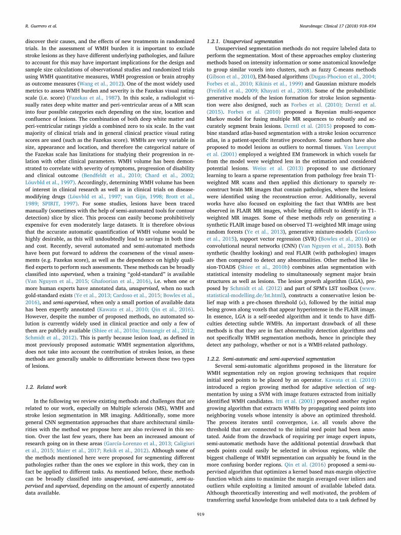
Fig. 6 shows Bland-Altman plots that further compare expert andautomatic WMH volumes. In these plots, the horizontal axis gives theaverage between expert and automatic volumes for each subject, whilethe vertical axis shows the difference between these volumes. The re-producibility coefficient (RPC), as calculated here, gives a measure ofthe variability (or spread) of the differences between automatic andmanual volumes and is calculated as 1.96 times the standard deviationσ of those differences (1.96 * σ). In the experiments presented here,smaller values indicate better agreement between automatic andmanual volumes. The coefficient of variation (CV) is given by σ X100* / ,where X refers to the mean volume from both measurements. Dottedlines in the plots of Fig. 6 give the range of the RPC. Bland-Altman plotsalso provide insight into possible biases of compared methods. LGAdisplays a statistically significant (p=0.85 to reject zero mean hy-pothesis) tendency to under-estimate volumes (central solid line).However, all methods tend to under-estimate larger volumes and over-estimate small ones, with the effect more pronounced in LGA.

One of the main objectives of the work presented here is to alsodifferentiate between WMH and stroke lesions. Neither LPA nor LGAare capable of making such a distinction, and therefore are not suitablealgorithms for this problem. Fig. 7 (top-row) shows the correlationanalysis between automatic (uResNet and DeepMedic) and expert

Table 2Mean Dice scores of WMH and stroke (standard deviation in parenthesis), correlationanalysis between expert and automatic volumes (R2 and trend), and correlation withclinical variables.

uResNet DeepMedic LPA LGA Expert

WMH Dice(std)

69.5(16.1) 66.6(16.7) 64.7(19.0) 41.0(22.9) −

Stroke Dice(std)

40.0(25.2) 31.3(29.2) − − −

WMH R2 0.951 0.943 0.855 0.687 −Stroke R2 0.791 0.688 − − −WMH Trend 0.89x+0.07 0.91x-0.06 0.83x+0.28 0.51x+0.16 −Stroke Trend 0.58x+0.01 0.52x-0.00 − − −CC D-Fazekas 0.770 0.769 0.746 0.630 0.774CC PV-Fazekas 0.778 0.780 0.777 0.718 0.765CC Fazekas 0.824 0.824 0.811 0.734 0.819CC MMSE 0.364 0.369 0.443 0.389 0.372

Fig. 5. Automated versus expertly generated WMH vo-lumes (as ICV %). The solid line indicates the linear trend f(x) of the comparison, while the dotted line indicates theideal trend f(x)=1.0x+0.0.

R. Guerrero et al. NeuroImage: Clinical 17 (2018) 918–934

926

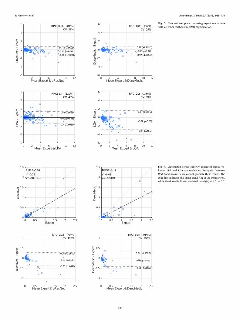
Fig. 6. Bland-Altman plots comparing expert annotationswith all other methods in WMH segmentation.

Fig. 7. Automated versus expertly generated stroke vo-lumes. LPA and LGA are unable to distinguish betweenWMH and stroke, hence cannot generate these results. Thesolid line indicates the linear trend f(x) of the comparison,while the dotted indicates the ideal trend f(x)=1.0x+0.0.

R. Guerrero et al. NeuroImage: Clinical 17 (2018) 918–934

927

stroke volumes (normalized as ICV). It is evident that uResNet out-performs DeepMedic in terms of RMSE, R2 and linear fit slope. Furtherto this analysis, Fig. 7 (bottom-row) shows Bland-Altman plots thatfurther confirm these findings, where uResNet obtains a smaller RPCand CV than DeepMedic, with neither method on average displaying astatistically significant tendency to over- or under-estimate volumes(see central solid line on plots). However, it is worth noting that bothmethods have a tendency to over-estimate small volumes and under-estimate larger ones. A summary of Figs. 5 and 7 is also presented inTable 2, where a difference between both algorithms in terms of Dicescores can be observed. Statistical significance between the comparisonof uResNet and DeepMedic Dice scores was found to be p<0.05 ac-cording to Wilcoxon's signed rank, with an effect size related to thisstatistical significance (as suggested by Pallant (2010)) of 0.12. The gapbetween uResNet and DeepMedic can be considerably closed if addi-tional inputs are provided to DeepMedic (see Appendix B), however thisrequires an additional MR image acquisition (and co-registration ofsuch image), tissue segmentation and/or co-registration of a cerebro-spinal track atlas. Furthermore, in Appendix C results of DeepMedicexperiments that aim to approximate the sampling scheme used byuResNet are discussed.

Fig. 8 shows the segmentation results from three example subjectsthat illustrate the differences between the methods. Here, it can beobserved that uResNet generally does a better job at differentiatingbetween WMH and stroke lesions when compared to DeepMedic (topand middle row). In the bottom row of Fig. 8 an example is illustratedwhen uResNet wrongly segments some WMH as stroke. Additionally, inthe top row, all methods are shown to clearly under-segment the imagewhen compared to the expert is shown. However, inspecting the FLAIRimage of this subject (top row, leftmost column) it can be seen that theunder-segmented regions would be challenging even for another expertannotator.

4.3. Clinical evaluation

Experiments thus far indicate a better agreement between volumesgenerated by uResNet and expert annotations, however, the question ofthe clinical validity of such results remains open. In this regard, Table 2gives correlation coefficient (CC) results between the volumes and someclinical variables (Fazekas scores and MMSE). Fazekas scores were splitinto deep white matter (D-Fazekas) and peri-ventricular (PV-Fazekas),with values ranging from 0 to 3. An additional combined Fazekas score,created by adding both D-Fazekas and PV-Fazekas, is also presented.From Table 2 we can observe that in terms of correlation to Fazekasscore the proposed uResNet outperforms the other competing methods,additionally noting that CC results for PV-Fazekas and Fazekas are evenhigher than those obtained from the expert annotations. However, interms of CC with MMSE it was LPA that performed best.

Using the clinical scores as well as known risk factors available, ananalysis of association between WMH volumes and risk factors wascarried out. In order to explore such associations a GLM between theresults of every algorithm (as well as the expert) and the risk factorswas generated. In these models, the risk factors and clinical scores weretreated as dependent variables, while the volumes acted as the in-dependent variable. After careful consideration, age, sex, reporteddiabetes, reported hypertension, reported hyperlipidaemia, reportedsmoking, total cholesterol, deep atrophy volume and BGPVS score wereused in the GLM analysis. Table 3 provides p-values that indicate if aparticular risk factor associated with the generated WMH volumes,where the GLMs were corrected for gender differences. Results indicatethat only BGPVS is found to be associated with the expertly generatedvolumes, however deep atrophy volume was also found to be associatedwith all other methods. Additionally, LPA volumes were also found tobe associated with age and diabetes.

In GLM analysis, values that are not well described by the model

Fig. 8. Visual comparisons of all competing methods. Yellow lines delineate WMH, green lines stroke and white arrows point to interesting result areas. Best seen in color.

R. Guerrero et al. NeuroImage: Clinical 17 (2018) 918–934

928

(outliers) can have a significant impact in subsequent analyses. Outliersin GLM can be identified by examining the probability distribution ofthe residuals. In order to eliminate any potential bias introduced byoutliers, an analysis with outliers removed was performed. Results ofthis outlier-free association analysis are presented in Table 4. Fig. 9shows the normal probability plot of residuals for all methods beforeand after outlier removal. From Table 4 we can observe that onceoutliers were removed, expert volumes were found to be associatedwith deep atrophy volume, BGPVS and diabetes. The same associationswere found for uResNet, DeepMedic and LPA, with the addition thatLPA was again also associated with age. LGA was found to only beassociated with BGPVS and deep atrophy volume.

Fazekas scores are highly co-linear with WMH volume (the depen-dent variable) and therefore were excluded from all previous GLManalysis. Nonetheless, a GLM that included Fazekas scores was alsocomposed as a sanity check that the correct associations would befound. A single Fazekas score was generated by adding the D-Fazekasand PV-Fazekas scores (0–6 score scale). All models found a very strongassociation (p≪ 0.001) between Fazekas and WMH volumes. The effectsize for the association of Fazekas score with the expertly generatedWMH volumes indicates that a change of one in the Fazekas scale,translates to a change of 0.75 ICV % increase of WMHs (1–0.75).DeepMedic obtained the closest effect size of the association betweenFazekas scores and WMH volumes to that of the expert, with a pre-diction that an increase of one Fazekas point produces 0.70 ICV % in-crease of WMH (1–0.70). uResNet closely followed with 1–0.69 pre-dictions. LPA and LGA results produced effect sizes of 1–0.6 and 1–0.35,respectively. Of the expert stroke lesion volumes, systolic blood pres-sure was the only risk factor to be found associated (p<0.05), whichincidentally was also associated with the automatically (uResNet andDeepMedic) generated volumes. uResNet values were additionallyfound to be associated with hypertension. However, it is important tonote the small size and heterogeneous nature of the population used inthis analysis, which might not prove sufficient to uncover some asso-ciations. Due to the small sample analyzed no outlier removal analysiswas performed for stroke associations.

5. Discussion

In this work we have proposed a CNN framework, uResNet, for thesegmentation of WMHs that is capable of distinguishing between WMHsarising from different pathologies, mainly WMHs of presumed VDorigin and those from stroke lesions. Comparison results indicate thatthe proposed uResNet architecture outperforms other well establishedand state-of-the-art algorithms.

The architecture used in uResNet follows closely the architecture ofU-Net Ronneberger et al. (2015). The main difference being the use ofresidual elements and a generally lower complexity through the use ofsummation instead of concatenation in skip connections. Preliminaryexperiments with both summation and concatenation of features mapsfound no difference in performance, hence low complexity was favored.However, it is also noted that a more general solution is given by theuse of concatenation, as this would allow the network to learn which isthe best way of combining the feature maps during training. Of coursethis additional complexity comes at the expense of a higher risk of over-fitting and a higher memory consumption. As mentioned, the use ofresidual units provides advantages during training, mainly improvedconvergence rates in our experiments. Recently, He et al. (2016b)proposed a new pre-activated residual unit, which optimizes the ar-chitecture of each unit making training easier and improving general-ization. Future work will involve updating the architecture to includesuch residual elements and evaluating their merits in the context ofWMH segmentation.

Large class imbalance in medical image segmentation is generallyan issue that must be considered. Loss functions that take into accountthe class imbalance have the drawback that they have the additionalclass weighting parameter to tune. An additional complication resultingfrom a large class imbalance is that a lot of computational effort mightbe spent optimizing to perform well in large and relatively easy toclassify/segment sections of an image. Bootstrapped cross-entropy at-tempts to focus the learning process on hard to classify parts of animage by dropping out loss function contribution from voxels that havealready been classified to a good degree of certainty. However, thistechnique also requires the setting of an additional parameter, thethreshold to consider a classification as already good, and moreover,evaluation results indicated a performance similar to classical cross-entropy.

A very important factor of the proposed CNN framework is thetraining data sampling strategy described in Section 2.3. CNN trainingfor medical imaging using patches is a somewhat standard techniquethat helps reduce the very large class imbalance that usually affectsmedical image segmentation. However, careful consideration must begiven in the sampling strategy adopted for a certain architecture. Asmentioned, class imbalance and lesion location within samples need tobe considered. The use of the proposed sampling strategy described inSection 2.3 had a profound effect on the proposed uResNet, with WMHand stroke Dice scores increasing from ∼67 to ∼70 and from ∼29 to∼40, respectively, due to this alone. Another important factor is thefrequency each class is sampled. In this work we sampled at 20% of thelocations labeled as WMH while at 80% of the locations labeled asstroke, again to try to balance classes. It is important to note that thedefault sampling settings of DeepMedic were used as in Kamnitsas et al.(2017). In this default sampling strategy, DeepMedic samples equallyfrom healthy and diseased tissues (that is without, considering fre-quency of different diseased classes) and furthermore does not includethe central voxel offset sampling strategy used here. We believe boththese factors had a significant impact in the differences between thesemethods, specially in the stroke lesion class. Training data was aug-mented by applying random flips to training patches, however we didnot find this had a clear effect on results.

An important aspect to note is that WMH segmentation is notor-iously challenging: For example, Bartko (1991) and Anbeek et al.(2004b) consider similarity scores of 70 to be excellent, while Landis

Table 3P-values of linear regression associations between volumes calculated with differentmethods and risk factors. Bold numbers indicate statistical significance above 0.05.

uResNet DeepMedic LPA LGA Expert

Age 0.491 0.533 < 0.001 0.723 0.313Diabetes 0.082 0.072 0.003 0.070 0.066Hyperlipidaemia 0.645 0.547 0.551 0.687 0.728Hypertension 0.820 0.781 0.504 0.358 0.562Smoking 0.497 0.560 0.216 0.719 0.767totalChl 0.235 0.281 0.161 0.328 0.371BGPVS < 0.001 < 0.001 < 0.001 < 0.001 < 0.001deepAtrophyVol 0.015 0.019 < 0.001 < 0.001 0.117

Table 4P-values of linear regression associations between volumes calculated with differentmethods and risk factors after residual outliers were removed. Bold numbers indicatestatistical significance above 0.05.

uResNet DeepMedic LPA LGA Expert

Age 0.905 0.993 < 0.001 0.685 0.407Diabetes 0.012 0.019 < 0.001 0.177 0.003Hyperlipidaemia 0.346 0.425 0.464 0.550 0.186Hypertension 0.639 0.502 0.190 0.128 0.350Smoking 0.069 0.084 0.107 0.673 0.343totalChl 0.294 0.212 0.222 0.043 0.868BGPVS < 0.001 < 0.001 < 0.001 < 0.001 < 0.001deepAtrophyVol 0.005 0.008 < 0.001 < 0.001 0.020

R. Guerrero et al. NeuroImage: Clinical 17 (2018) 918–934

929

and Koch (1977) consider scores of 40, 60 and 80 to be moderate,substantial and near perfect, respectively. With this in mind, we canconsider average Dice scores for WMHs generated by the proposeduResNet, as well as those from DeepMedic and LPA to all be substantial,with LGA generating only moderate results. It is important to note thatLGA is at heart an unsupervised method and that data was only used totune its κ parameter. Only uResNet and DeepMedic are capable ofdistinguishing between different types of lesion, and in this regard onlyuResNet produced an average stroke Dice score that could be con-sidered moderate.

Acknowledgments

The research presented here was partially funded by Innovate UK(formerly UK Technology Strategy Board) grant no. 102167 and by the7th Framework Programme by the European Commission (http://cordis.europa.eu; EU-grant-611005-PredictND – From Patient Data toClinical Diagnosis in Neurodegenerative Diseases). Additionally, dataused in preparation of this work was obtained under funding by theRow Fogo Charitable Trust (AD.ROW4.35. BRO-D.FID3668413) forMVH, and the Wellcome Trust (WT088134/Z/09/A).

Fig. 9. General linear model normal probability plots of residuals for all methods, with and without outliers.

R. Guerrero et al. NeuroImage: Clinical 17 (2018) 918–934

930

Appendix A. Variations of uResNet

In this section we present results comparing the proposed architecture and sampling scheme, with two additional version: One where theresidual block takes the more traditional form of two convolutional elements (called uResNet2) and another where the proposed center shiftingsampling scheme is replaced with a standard centered patch sampling scheme (called uResNet_NoC, for not off-centered). Table A.5 summarizesthese results.

Using single convolution residual blocks was noted (He et al., 2016a) to be equivalent to a linear projection. After experimented with residualsblocks of one and two convolutions, we observed no statistical difference (p>0.05) between them. However, learning the residual of these linearprojections might still be simpler, thus leading to an observed faster convergence. This observations need to be interpreted with care. We believe thatthe Dice overlap scores that our method achieves are close to expected intra-rater variability, hence the lack of observed difference in performancebetween one and two convolutions in residual blocks, might come down to limitations of the data itself.

Training with patches that always contain a diseased label in the center would bias towards labeling this region of a patch as diseased duringinference. Patch center shifting alleviates this problem due to the distribution of probability to observe a lesion across the whole field-of-view. Forexample, if we would estimate the probability of observing a lesion in any particular location of a training patch, there would be 100% probabilityto observe a lesion at its center (Fig. A.10 (a)), as we explicitly sampled in this manner. Allowing patches to be shifted spreads this probability toall locations and not any single location has a preferential likelihood of being a lesion (Fig. A.10 (b)). In a fully convolutional neural networkpredictions can be made over a large area (as the network proposed here), taking into account context information from large areas of an image(the field-of-view or receptive field). However, training is driven by pixel-wise prediction errors, hence labeling occurs on a per-pixel basis. Thelikelihood of observing a lesion at any particular location is in fact very low (see Fig. A.10 (b)) and more or less uniform. It is this uniformity thatremoves the bias towards any particular location. Results comparing a uResNet with out center shifting sampling are shown in Table A.5.

Table A.5Mean Dice scores of WMH and stroke (standard deviation in parenthesis), correlation analysis between expert and automatic volumes (R2 andtrend), and correlation with clinical variables. No statistical significance between uResNet and uResNet2 was observed (p>0.05), while therewas a statistically significant difference (p<0.001) between patch off-center sampling (uResNet) and regular no off-center sampling(uResNet_NoC).

uResNet uResNet2 uResNet_NoC Expert

WMH Dice (std) 69.5(16.1) 69.6(16.1) 66.9(18.1) −Stroke Dice (std) 40.0(25.2) 40.2(27.7) 28.9(22.3) −WMH R2 0.951 0.951 0.948 −Stroke R2 0.791 0.761 0.710 −WMH Trend 0.89x+0.07 0.89x-0.08 0.89x+0.15 −Stroke Trend 0.58x+0.01 0.55x-0.01 0.52x+0.07 −CC D-Fazekas 0.770 0.776 0.771 0.774CC PV-Fazekas 0.778 0.783 0.777 0.765CC Fazekas 0.824 0.831 0.823 0.819CC MMSE 0.364 0.373 0.366 0.372

Fig. A.10. Lesion likelihood on training patches (a) without shifting and (b) after shifting.

Appendix B. Dice results for different inputs

Both CNN approaches, uResNet and DeepMedic, can easily be trained using one or several inputs. Table B.6 provides Dice overlap results of usingdifferent input channels in both CNN approaches. As it can be appreciated DeepMedic can narrow the Dice overlap gap with uResNet if several inputsare provided. However, as discussed before, obtaining and generating these extra inputs limit clinical applicability and also add additional com-putational costs to the whole segmentation framework.

R. Guerrero et al. NeuroImage: Clinical 17 (2018) 918–934

931

Table B.6Mean Dice scores of WMH and stroke, for different inputs with uResNet and DeepMedic. Difference in Dice score between the two methods is given initalics. F: FLAIR image, CS: cerebro-spinal track atlas, WM: white matter probability map, T1: T1 weighted image.

Input WMH Stroke

channels uResNet DeepMedic Diff uResNet DeepMedic Diff

F 69.5 66.3 3.2 40.0 31.1 8.9F-T1 69.7 67.6 2.1 35.5 34.3 1.2F-CS 69.1 66.6 2.5 36.7 35.1 1.6F-WM 69.4 68.2 1.2 33.0 35.9 − 2.9F-CS-WM 69.3 68.0 1.3 38.4 37.8 0.6F-T1-CS-WM 69.6 68.4 1.2 40.2 36.0 4.2

Appendix C. Additional DeepMedic experiments

DeepMedic experiments that aim to approximate the sampling scheme used by uResNet were carried out, where several sampling weights weretested for DeepMedic. A direct comparison of per-class patch sampling is not straightforward between the proposed method and DeepMedic, andfurthermore it can be misleading. For instance, in the work proposed here a sampling rate of 80–20% of WHM-stroke patches is used, each patch hasa size of 64 by 64 voxels and uResNet makes a prediction of a 64 by 64 patch of the label space during training (it is fully convolutional and usespadded convolutions throughout). This means that each patch used in uResNet has a label map that due to its size inevitably contains a large amountof healthy tissue. Therefore we do not sample specifically from healthy regions. On the other hand, DeepMedic trains with segments that have a labelspace of 9 by 9 by 9 voxels, therefore it is far less likely that healthy tissue is included in non-healthy samples and thus healthy segments need to besampled. Nonetheless, different per-class sampling rates, as well as other hyper-parameter settings with DeepMedic were explored.

Some of DeepMedic's default hyper-parameter values are: learning rate of 1e-3, RmsProp optimizer, sampling form of foreground/background(diseased/healthy tissue) and sampling rate of [0.5, 0.5] (healthy and diseased tissue). The different sampling rates tested with DeepMedic in ourexperiments to approximate uResNet setup were [0.5, 0.1, 0.4], [0.5, 0.25, 0.25], [0.33, 0.13, 0.53] and [0.33, 0.33, 0.3], for healthy, WMH andstroke tissue, respectively. Additionally, learning rate values explored were in the range of 1.9e-2 to 1e-4, with RMSprop, Adam or SGD as optimizer.Changing the sampling rates from the default generally produced unstable results, with either failing to converge or producing poorer overlap valuesthan with the default settings. In total, 14 different additional DeepMedic train/test runs were performed, out of which only two converged, bothusing a sampling rate of [0.33, 0.33,0.33]. Dice overlap results by these experiments were of 60.7 and 29.9, for WMH and stroke, respectively, in oneinstance and 59.4 and 29.5 in the other. These unstable results might be due to the tuning of additional meta parameters, such as the optimizer,learning rate or regularization. Therefore, presented DeepMedic results were obtained with default hyper-parameters, which were the best resultsobtained in our experiments.

References

SPIRIT, 1997. A randomized trial of anticoagulants versus aspirin after cerebral ischemiaof presumed arterial origin. The Stroke Prevention in Reversible Ischemia Trial(SPIRIT) Study Group. Ann. Neurol. 42 (6), 857–865.

Al-Rfou, R., Alain, G., Almahairi, A., Angermueller, C., Bahdanau, D., Ballas, N., Bastien,F., Bayer, J., Belikov, A., Belopolsky, A., Bengio, Y., Bergeron, A., Bergstra, J., Bisson,V., Bleecher Snyder, J., Bouchard, N., Boulanger-Lewandowski, N., Bouthillier, X., deBrébisson, A., Breuleux, O., Carrier, P.-L., Cho, K., Chorowski, J., Christiano, P.,Cooijmans, T., Côté, M.-A., Côté, M., Courville, A., Dauphin, Y.N., Delalleau, O.,Demouth, J., Desjardins, G., Dieleman, S., Dinh, L., Ducoffe, M., Dumoulin, V.,Ebrahimi Kahou, S., Erhan, D., Fan, Z., Firat, O., Germain, M., Glorot, X., Goodfellow,I., Graham, M., Gulcehre, C., Hamel, P., Harlouchet, I., Heng, J.-P., Hidasi, B., Honari,S., Jain, A., Jean, S., Jia, K., Korobov, M., Kulkarni, V., Lamb, A., Lamblin, P., Larsen,E., Laurent, C., Lee, S., Lefrancois, S., Lemieux, S., Léonard, N., Lin, Z., Livezey, J.A.,Lorenz, C., Lowin, J., Ma, Q., Manzagol, P.-A., Mastropietro, O., McGibbon, R.T.,Memisevic, R., van Merriënboer, B., Michalski, V., Mirza, M., Orlandi, A., Pal, C.,Pascanu, R., Pezeshki, M., Raffel, C., Renshaw, D., Rocklin, M., Romero, A., Roth, M.,Sadowski, P., Salvatier, J., Savard, F., Schlüter, J., Schulman, J., Schwartz, G.,Serban, I.V., Serdyuk, D., Shabanian, S., Simon, E.,́ Spieckermann, S., Subramanyam,S.R., Sygnowski, J., Tanguay, J., van Tulder, G., Turian, J., Urban, S., Vincent, P.,Visin, F., de Vries, H., Warde-Farley, D., Webb, D.J., Willson, M., Xu, K., Xue, L., Yao,L., Zhang, S., Zhang, Y., 2016. Theano: A {Python} framework for fast computation ofmathematical expressions. arXiv e-prints, abs/1605.02688, may.

Anbeek, P., Vincken, K.L., Van Osch, M.J., Bisschops, R.H., Van Der Grond, J., 2004a.Probabilistic segmentation of white matter lesions in MR imaging. NeuroImage 21(3), 1037–1044.

Anbeek, P., Vincken, K.L., van Osch, M.J., Bisschops, R.H., van der Grond, J., 2004b.Probabilistic segmentation of white matter lesions in MR imaging. NeuroImage 21(3), 1037–1044.

Bartko, J.J., 1991. Measurement and reliability: statistical thinking considerations.Schizophr. Bull. 17 (3), 483–489.

Bendfeldt, K., Blumhagen, J.O., Egger, H., Loetscher, P., Denier, N., Kuster, P., Traud, S.,Mueller-Lenke, N., Naegelin, Y., Gass, A., Hirsch, J., Kappos, L., Nichols, T.E., Radue,E.-W., Borgwardt, S.J., 2010. Spatiotemporal distribution pattern of white matterlesion volumes and their association with regional grey matter volume reductions in

relapsing-remitting multiple sclerosis. Hum. Brain Mapp. 31 (10), 1542–1555 (oct).Birenbaum, A., Greenspan, H., 2016. Longitudinal multiple sclerosis lesion segmentation

using multi-view convolutional neural networks. In: International Workshop onLarge-Scale Annotation of Biomedical Data and Expert Label Synthesis. Springer, pp.58–67.

Bowles, C., Qin, C., Ledig, C., Guerrero, R., Hammers, A., Sakka, E., Dickie, D.A., Tijms,B., Lemstra, A.W., Flier, W.V.D., 2016. Pseudo-healthy image synthesis for whitematter lesion segmentation. In: International Workshop on Simulation and Synthesisin Medical Imaging. vol. 9968. Springer International Publishing, pp. 87–96.

Brosch, T., Tang, L.Y., Yoo, Y., Li, D.K., Traboulsee, A., Tam, R., 2016. Deep 3d con-volutional encoder networks with shortcuts for multiscale feature integration appliedto multiple sclerosis lesion segmentation. IEEE Trans. Med. Imaging 35 (5),1229–1239.

Brosch, T., Yoo, Y., Tang, L.Y., Li, D.K., Traboulsee, A., Tam, R., 2015. Deep convolutionalencoder networks for multiple sclerosis lesion segmentation. In: InternationalConference on Medical Image Computing and Computer-Assisted Intervention.Springer, pp. 3–11.

Brott, T., Marler, J.R., Olinger, C.P., Adams, H.P., Tomsick, T., Barsan, W.G., Biller, J.,Eberle, R., Hertzberg, V., Walker, M., 1989. Measurements of acute cerebral infarc-tion: lesion size by computed tomography. Stroke 20 (7), 871–875.

Caligiuri, M.E., Perrotta, P., Augimeri, A., Rocca, F., Quattrone, A., Cherubini, A., 2015.Automatic detection of white matter hyperintensities in healthy aging and pathologyusing magnetic resonance imaging: a review. Neuroinformatics 13 (3), 261–276.

Cardoso, M.J., Sudre, C.H., Modat, M., Ourselin, S., 2015. Template-based multimodaljoint generative model of brain data. In: Information Processing in Medical Imaging.vol. 9123. Springer International Publishing, pp. 17–29.

Chard, D.T., Griffin, C.M., Parker, G.J.M., Kapoor, R., Thompson, A.J., Miller, D.H., 2002.Brain atrophy in clinically early relapsing-remitting multiple sclerosis. Brain J.Neurol. 125 (2), 327–337.

Cohen, J., 1988. Statistical Power Analysis for the Behavioral Sciences, 2nd edition.Lawrence Erlbaum Associates, pp. 40.

Dalca, A.V., Sridharan, R., Cloonan, L., Fitzpatrick, K.M., Kanakis, A., Furie, K.L., Rosand,J., Wu, O., Sabuncu, M., Rost, N.S., et al., 2014. Segmentation of cerebrovascularpathologies in stroke patients with spatial and shape priors. In: Medical imagecomputing and computer-assisted intervention: MICCAI. International Conference onMedical Image Computing and Computer-Assisted Intervention. vol. 17. pp. 773.

Damangir, S., Manzouri, A., Oppedal, K., Carlsson, S., Firbank, M.J., Sonnesyn, H.,

R. Guerrero et al. NeuroImage: Clinical 17 (2018) 918–934

932

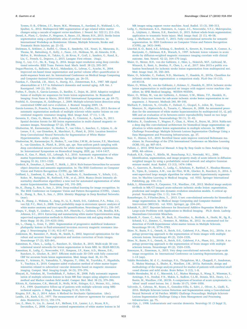
Tysnes, O.-B., O’Brien, J.T., Beyer, M.K., Westman, E., Aarsland, D., Wahlund, L.-O.,Spulber, G., 2012. Multispectral MRI segmentation of age related white matterchanges using a cascade of support vector machines. J. Neurol. Sci. 322 (1), 211–216.

Derntl, A., Plant, C., Gruber, P., Wegener, S., Bauer, J.S., Menze, B.H., 2015. Stroke lesionsegmentation using a probabilistic atlas of cerebral vascular territories. In:International Workshop on Brainlesion: Glioma, Multiple Sclerosis, Stroke andTraumatic Brain Injuries, pp. 21–32.

Dieleman, S., Schlüter, J., Raffel, C., Olson, E., Sønderby, S.K., Nouri, D., Maturana, D.,Thoma, M., Battenberg, E., Kelly, J., Fauw, J.D., Heilman, M., de Almeida, D.M.,McFee, B., Weideman, H., Takács, G., de Rivaz, P., Crall, J., Sanders, G., Rasul, K.,Liu, C., French, G., Degrave, J., 2015. Lasagne: First release. (Aug).

Dong, C., Loy, C.C., He, K., Tang, X., 2016. Image super-resolution using deep convolu-tional networks. IEEE Trans. Pattern Anal. Mach. Intell. 38 (2), 295–307.

Dugas-Phocion, G., Ballester, M.A.G., Malandain, G., Lebrun, C., Ayache, N., 2004.Improved em-based tissue segmentation and partial volume effect quantification inmulti-sequence brain mri. In: International Conference on Medical Image Computingand Computer-Assisted Intervention. Springer, pp. 26–33.

Fazekas, F., Chawluk, J.B., Alavi, A., Hurtig, H.I., Zimmerman, R.A., 1987. MR signalabnormalities at 1.5 T in Alzheimer's dementia and normal aging. AJR Am. J.Roentgenol. 149 (2), 351–356.

Forbes, F., Doyle, S., Garcia-Lorenzo, D., Barillot, C., Dojat, M., 2010. Adaptive weightedfusion of multiple mr sequences for brain lesion segmentation. In: BiomedicalImaging: From Nano to Macro, 2010 IEEE International Symposium on, pp. 69–72.

Freifeld, O., Greenspan, H., Goldberger, J., 2009. Multiple sclerosis lesion detection usingconstrained GMM and curve evolution. J. Biomed. Imaging 2009, 14.

García-Lorenzo, D., Francis, S., Narayanan, S., Arnold, D.L., Collins, D.L., 2013. Review ofautomatic segmentation methods of multiple sclerosis white matter lesions on con-ventional magnetic resonance imaging. Med. Image Anal. 17 (1), 1–18.

Geremia, E., Clatz, O., Menze, B.H., Konukoglu, E., Criminisi, A., Ayache, N., 2011.Spatial decision forests for MS lesion segmentation in multi-channel magnetic re-sonance images. NeuroImage 57 (2), 378–390.

Ghafoorian, M., Karssemeijer, N., Heskes, T., van Uden, I., Sanchez, C., Litjens, G., deLeeuw, F.-E., van Ginneken, B., Marchiori, E., Platel, B., 2016. Location SensitiveDeep Convolutional Neural Networks for Segmentation of White MatterHyperintensities. ArXiv e-prints, Oct.

Ghafoorian, M., Karssemeijer, N., Heskes, T., van Uder, I.W.M., de Leeuw, F.E., Marchiori,E., van Ginneken, B., Platel, B., 2016, apr, apr. Non-uniform patch sampling withdeep convolutional neural networks for white matter hyperintensity segmentation.In: International Symposium on Biomedical Imaging. IEEE, pp. 1414–1417.

Gibson, E., Gao, F., Black, S.E., Lobaugh, N.J., 2010. Automatic segmentation of whitematter hyperintensities in the elderly using flair images at 3t. J. Magn. Reson.Imaging 31 (6), 1311–1322.

Girshick, R., Donahue, J., Darrell, T., Malik, J., 2014. Rich feature hierarchies for accurateobject detection and semantic segmentation. In: The IEEE Conference on ComputerVision and Pattern Recognition (CVPR), pp. 580–587.

Griffanti, L., Zamboni, G., Khan, A., Li, L., Bonifacio, G., Sundaresan, V., Schulz, U.G.,Kuker, W., Battaglini, M., Rothwell, P.M., et al., 2016. Bianca (brain intensity ab-normality classification algorithm): a new tool for automated segmentation of whitematter hyperintensities. Neuroimage 141, 191–205.

He, K., Zhang, X., Ren, S., Sun, J., 2016. Deep residual learning for image recognition. In:The IEEE Conference on Computer Vision and Pattern Recognition (CVPR), (June).

He, K., Zhang, X., Ren, S., Sun, J., 2016. Identity Mappings in Deep Residual Networks.(mar).

Hua, K., Zhang, J., Wakana, S., Jiang, H., Li, X., Reich, D.S., Calabresi, P.A., Pekar, J.J.,van Zijl, P.C., Mori, S., 2008. Tract probability maps in stereotaxic spaces: analyses ofwhite matter anatomy and tract-specific quantification. NeuroImage 39 (1), 336–347.

Ithapu, V., Singh, V., Lindner, C., Austin, B.P., Hinrichs, C., Carlsson, C.M., Bendlin, B.B.,Johnson, S.C., 2014. Extracting and summarizing white matter hyperintensities usingsupervised segmentation methods in Alzheimer's disease risk and aging studies. Hum.Brain Mapp. 35 (8), 219–4235 (feb).

Itti, L., Chang, L., Ernst, T., 2001. Segmentation of progressive multifocal leukoence-phalopathy lesions in fluid-attenuated inversion recovery magnetic resonance ima-ging. J. Neuroimaging 11 (4), 412–417 (oct).

Jenkinson, M., Bannister, P., Brady, M., Smith, S., 2002. Improved optimization for therobust and accurate linear registration and motion correction of brain images.NeuroImage 17 (2), 825–841.

Kamnitsas, K., Chen, L., Ledig, C., Rueckert, D., Glocker, B., 2015. Multi-scale 3D con-volutional neural networks for lesion segmentation in brain MRI. In: ISLES-MICCAI.

Kamnitsas, K., Ledig, C., Newcombe, V.F., Simpson, J.P., Kane, A.D., Menon, D.K.,Rueckert, D., Glocker, B., 2017. Efficient multi-scale 3D CNN with fully connectedCRF for accurate brain lesion segmentation. Med. Image Anal. 36, 61–78.

Kawata, Y., Arimura, H., Yamashita, Y., Magome, T., Ohki, M., Toyofuku, F., Higashida,Y., Tsuchiya, K., 2010. Computer-aided evaluation method of white matter hyper-intensities related to subcortical vascular dementia based on magnetic resonanceimaging. Comput. Med. Imaging Graph. 34 (5), 370–376.

Khayati, R., Vafadust, M., Towhidkhah, F., Nabavi, M., 2008. Fully automatic segmen-tation of multiple sclerosis lesions in brain MR flair images using adaptive mixturesmethod and Markov random field model. Comput. Biol. Med. 38 (3), 379–390.

Kikinis, R., Guttmann, C.R., Metcalf, D., Wells, W.M., Ettinger, G.J., Weiner, H.L., Jolesz,F.A., 1999. Quantitative follow-up of patients with multiple sclerosis using MRI:technical aspects. J. Magn. Reson. Imaging 9 (4), 519–530.

Kingma, D.P., Ba, J., 2014. Adam: A Method for Stochastic Optimization. (dec).Landis, J.R., Koch, G.G., 1977. The measurement of observer agreement for categorical

data. Biometrics 33 (1), 159–174.Lao, Z., Shen, D., Liu, D., Jawad, A.F., Melhem, E.R., Launer, L.J., Bryan, R.N.,

Davatzikos, C., 2008. Computer-assisted segmentation of white matter lesions in 3d

MR images using support vector machine. Acad. Radiol. 15 (3), 300–313.Ledig, C., Heckemann, R.A., Hammers, A., Lopez, J.C., Newcombe, V.F.J., Makropoulos,

A., Lötjönen, J., Menon, D.K., Rueckert, D., 2015. Robust whole-brain segmentation:application to traumatic brain injury. Med. Image Anal. 21 (1), 40–58.

Long, J., Shelhamer, E., Darrell, T., 2015. Fully convolutional networks for semanticsegmentation. In: IEEE Conference on Computer Vision and Pattern Recognition(CVPR), pp. 3431–3440.

Löuvbld, K.-O., Baird, A.E., Schlaug, G., Benfield, A., Siewert, B., Voetsch, B., Connor, A.,Burzynski, C., Edelman, R.R., Warach, S., 1997. Ischemic lesion volumes in acutestroke by diffusion-weighted magnetic resonance imaging correlate with clinicaloutcome. Ann. Neurol. 42 (2), 164–170 (aug).

Maier, O., Menze, B.H., von der Gablentz, J., Häni, L., Heinrich, M.P., Liebrand, M.,Winzeck, S., Basit, A., Bentley, P., Chen, L., et al., 2017. Isles 2015-a public eva-luation benchmark for ischemic stroke lesion segmentation from multispectral mri.Med. Image Anal. 35, 250–269.

Maier, O., Schröder, C., Forkert, N.D., Martinetz, T., Handels, H., 2015a. Classifiers forischemic stroke lesion segmentation: a comparison study. PLoS One 10 (12),e0145118.

Maier, O., Wilms, M., von der Gablentz, J., Krämer, U., Handels, H., 2014. Ischemic strokelesion segmentation in multi-spectral mr images with support vector machine clas-sifiers. In: SPIE Medical Imaging, 903504–903504.

Maier, O., Wilms, M., von der Gablentz, J., Krämer, U.M., Münte, T.F., Handels, H.,2015b. Extra tree forests for sub-acute ischemic stroke lesion segmentation in mrsequences. J. Neurosci. Methods 240, 89–100.

Maillard, P., Delcroix, N., Crivello, F., Dufouil, C., Gicquel, S., Joliot, M., Tzourio-Mazoyer, N., Alpérovitch, A., Tzourio, C., Mazoyer, B., 2008. An automated proce-dure for the assessment of white matter hyperintensities by multispectral (t1, t2, pd)MRI and an evaluation of its between-centre reproducibility based on two largecommunity databases. Neuroradiology 50 (1), 31–42.

McKinley, R., Gundersen, T., Wagner, F., Chan, A., Wiest, R., Reyes, M., 2016. Nabla-net:a deep dag-like convolutional architecture for biomedical image segmentation: ap-plication to white-matter lesion segmentation in multiple sclerosis. In: MSSEGChallenge Proceedings: Multiple Sclerosis Lesions Segmentation Challenge Using aData Management and Processing Infrastructure, pp. 37.

Nair, V., Hinton, G.E., 2010. Rectified linear units improve restricted Boltzmann ma-chines. In: Proceedings of the 27th International Conference on Machine Learning(ICML-10), pp. 807–814.

Pallant, J., 2010. SPSS Survival Manual: A Step By Step Guide to Data Analysis UsingSPSS, 4th edition. .

Prakash, K.B., Gupta, V., Bilello, M., Beauchamp, N.J., Nowinski, W.L., 2006.Identification, segmentation, and image property study of acute infarcts in diffusion-weighted images by using a probabilistic neural network and adaptive Gaussianmixture model. Acad. Radiol. 13 (12), 1474–1484.

Qin, C., Guerrero, R., Bowles, C., Ledig, C., Scheltens, P., Barkhof, F., Rhodius-Meester,H., Tijms, B., Lemstra, A.W., van der Flier, W.M., Glocker, B., Rueckert, D., 2016. Asemi-supervised large margin algorithm for white matter hyperintensity segmenta-tion. In: Machine Learning in Medical Imaging. vol. 9352. Springer InternationalPublishing, pp. 104–112.

Rekik, I., Allassonnière, S., Carpenter, T.K., Wardlaw, J.M., 2012. Medical image analysismethods in MR/CT-imaged acute-subacute ischemic stroke lesion: segmentation,prediction and insights into dynamic evolution simulation models. A critical ap-praisal. NeuroImage Clin. 1 (1), 164–178.

Ronneberger, O., P.Fischer,Brox, T., 2015. U-net: convolutional networks for biomedicalimage segmentation. In: Medical Image Computing and Computer-AssistedIntervention (MICCAI). vol. 9351. Springer, pp. 234–241.

Schmidt, P., 2017. Bayesian Inference for Structured Additive Regression Models forLarge-scale Problems with Applications to Medical Imaging. Ph.D. thesis. Ludwig-Maximilians-Universität München.

Schmidt, P., Gaser, C., Arsic, M., Buck, D., Förschler, A., Berthele, A., Hoshi, M., Ilg, R.,Schmid, V.J., Zimmer, C., Hemmer, B., Mühlau, M., 2012. An automated tool fordetection of FLAIR-hyperintense white-matter lesions in Multiple Sclerosis.NeuroImage 59 (4), 3774–3783.

Shiee, N., Bazin, P.-L., Ozturk, A., Reich, D.S., Calabresi, P.A., Pham, D.L., 2010a. A to-pology-preserving approach to the segmentation of brain images with multiplesclerosis lesions. NeuroImage 49 (2), 1524–1535.

Shiee, N., Bazin, P.-L., Ozturk, A., Reich, D.S., Calabresi, P.A., Pham, D.L., 2010b. A to-pology-preserving approach to the segmentation of brain images with multiplesclerosis lesions. NeuroImage 49 (2), 1524–1535.

Simonyan, K., Zisserman, A., 2015. Very deep convolutional networks for large-scaleimage recognition. In: International Conference on Learning Representations, pp.1–14 (sep).

Valdés Hernández, M. d. C., Armitage, P.A., Thrippleton, M.J., Chappell, F., Sandeman,E., Muñoz Maniega, S., Shuler, K., Wardlaw, J.M., 2015a. Rationale, design andmethodology of the image analysis protocol for studies of patients with cerebral smallvessel disease and mild stroke. Brain Behav. 5 (12), 1–8.

Valdés Hernández, M. d. C., Maconick, L.C., Muñoz Maniega, S., Wang, X., Wiseman, S.,Armitage, P.A., Doubal, F.N., Makin, S., Sudlow, C.L.M., Dennis, M.S., Deary, I.J.,Bastin, M., Wardlaw, J.M., 2015b. A comparison of location of acute symptomatic vs.‘silent’ small vessel lesions. Int. J. Stroke 10 (7), 1044–1050.

Valverde, S., Cabezas, M., Roura, E., González-Villa, S., Salvi, J., Oliver, A., Lladó, X.,2016. Multiple Sclerosis Lesion Detection and Segmentation using a ConvolutionalNeural Network of 3d Patches. MSSEG Challenge Proceedings: Multiple SclerosisLesions Segmentation Challenge Using a Data Management and ProcessingInfrastructure. pp. 75.

van Gijn, J., 1998. Leukoaraiosis and vascular dementia. Neurology 51 (3 Suppl 3),S3–S8.

R. Guerrero et al. NeuroImage: Clinical 17 (2018) 918–934

933

Van Leemput, K., Maes, F., Vandermeulen, D., Colchester, A., Suetens, P., 2001.Automated segmentation of multiple sclerosis lesions by model outlier detection.IEEE Trans. Med. Imaging 20 (8), 677–688.

Van Nguyen, H., Zhou, K., Vemulapalli, R., 2015. Cross-domain synthesis of medicalimages using efficient location-sensitive deep network. In: Medical Image Computingand Computer-Assisted Intervention. vol. 9349. Springer International Publishing,pp. 677–684.

Wang, X., Valdés Hernández, M.C., Doubal, F., Chappell, F.M., Wardlaw, J.M., 2012. Howmuch do focal infarcts distort white matter lesions and global cerebral atrophymeasures?. Cerebrovasc. Dis. (Basel, Switz.) 34 (5-6), 336–342.

Wardlaw, J.M., Pantoni, L., 2014. Sporadic Small Vessel Disease: Pathogenic Aspects.Cambridge University Press, Cambridge, pp. 52–63.

Wardlaw, J.M., Smith, E.E., Biessels, G.J., Cordonnier, C., Fazekas, F., Frayne, R., Lindley,R.I., O’Brien, J.T., Barkhof, F., Benavente, O.R., Black, S.E., Brayne, C., Breteler, M.,Chabriat, H., DeCarli, C., de Leeuw, F.-E., Doubal, F., Duering, M., Fox, N.C.,

Greenberg, S., Hachinski, V., Kilimann, I., Mok, V., van Oostenbrugge, R., Pantoni, L.,Speck, O., Stephan, B.C.M., Teipel, S., Viswanathan, A., Werring, D., Chen, C., Smith,C., van Buchem, M., Norrving, B., Gorelick, P.B., Dichgans, M., 2013. Neuroimagingstandards for research into small vessel disease and its contribution to ageing andneurodegeneration. Lancet Neurol. 12 (8), 822–838.

Weiss, N., Rueckert, D., Rao, A., 2013. Multiple sclerosis lesion segmentation using dic-tionary learning and sparse coding. In: International Conference on Medical ImageComputing and Computer-Assisted Intervention. 8149. pp. 735–742.

Wu, Z., Shen, C., Van Den Hengel, A., High-performance Semantic Segmentation UsingVery Deep Fully Convolutional Networks, ArXiv e-prints.

Ye, D.H., Zikic, D., Glocker, B., Criminisi, A., Konukoglu, E., 2013. Modality propagation:coherent synthesis of subject-specific scans with data-driven regularization. In:International Conference on Medical Image Computing and Computer-AssistedIntervention. vol. 8149. Springer Berlin Heidelberg, pp. 606–613.

R. Guerrero et al. NeuroImage: Clinical 17 (2018) 918–934

934