Image and Vision Computing 27 (2009) 588–596

Contents lists available at ScienceDirect

Image and Vision Computing

journal homepage: www.elsevier .com/locate / imavis

Edge landmarks in monocular SLAM

Ethan Eade *, Tom DrummondCambridge University, Cambridge CB2 1PZ, UK

a r t i c l e i n f o

Article history:Received 4 April 2007Received in revised form 3 October 2007Accepted 24 April 2008

Keywords:SLAMMonocular SLAMStructure and motionEdgesLandmarksParticle filterEdgeletPartial initializationInverse depthData associationSimultaneous localization and mappingEdge detectionMonocular vision

0262-8856/$ - see front matter � 2008 Elsevier B.V. Adoi:10.1016/j.imavis.2008.04.012

* Corresponding author. Tel.: +44 7990652373.E-mail addresses: ee231@cam.ac.uk (E. Eade), twd2

a b s t r a c t

While many visual simultaneous localization and mapping (SLAM) systems use point features as land-marks, few take advantage of the edge information in images. Those SLAM systems that do observe edgefeatures do not consider edges with all degrees of freedom. Edges are difficult to use in vision SLAMbecause of selection, observation, initialization and data association challenges. A map that includes edgefeatures, however, contains higher-order geometric information useful both during and after SLAM. Wedefine a well-localized edge landmark and present an efficient algorithm for selecting such landmarks.Further, we describe how to initialize new landmarks, observe mapped landmarks in subsequent images,and address the data association challenges of edges. Our methods, implemented in a particle-filter SLAMsystem, operate at frame rate on live video sequences.

� 2008 Elsevier B.V. All rights reserved.

1. Introduction

Much work in visual SLAM systems focuses on mapping point-based landmarks. Point landmarks have desirable properties in thecontext of visual SLAM: point feature selection and description arewell-studied, the resulting feature descriptors are well-localizablein images, and they are highly distinctive, easing the task of dataassociation. Many environments, however, have abundant edgesand edge-like features. By tracking edges in the world, a SLAM sys-tem can build richer maps containing higher-level geometric infor-mation, and need not rely on an abundance of good point features.In contrast to point features, edges are well-localizable in only oneimage dimension, and often have non-local extent in the otherimage dimension. Though highly invariant to lighting, edges arealso difficult to distinguish from each other locally. Such character-istics make the incorporation of edge landmarks into a visual SLAMsystem challenging.

This work focuses on SLAM with edges. We encourage the read-er to examine [2,18,13,9] for detailed discussions of the generaloperation of visual SLAM systems. Our work is implemented with-in the system described in [5].

ll rights reserved.

0@cam.ac.uk (T. Drummond).

Edges have been recognized as critical features in image pro-cessing since the beginning of computer vision. While edge detec-tion methods abound, Canny’s algorithm [1] for choosing edgels inan image has emerged as the standard technique, and consistentlyranks well in comparisons [8,17]. We use it as a starting point forour edge feature selection algorithm.

The invariance of edges to lighting, orientation, and scale makesthem good candidates for tracking. Model-based trackers such as[3] and [15] use edge models to permit highly efficient trackingof moving objects. Model-based tracking with edges, where struc-ture is known but camera or object position is unknown, can beconsidered a subset of our SLAM problem.

The structure-from-motion (SFM) algorithm described in [20]operates solely on edges detected in a video sequence. A global costfunction is optimized to yield camera trajectory and line parame-ters. Results of this work are also shown in [17]. There are twoimportant differences between such globally-optimized SFM andSLAM: SLAM must maintain estimates of camera motion and worldstructure online, not in a global optimization, and a SLAM systemmust maintain uncertainty information regarding its estimates ofmotion and structure.

The vision SLAM system of [6] is designed to support heteroge-neous landmark types in a common framework. While lines areused as features, they are assumed to be confined to planes of

E. Eade, T. Drummond / Image and Vision Computing 27 (2009) 588–596 589

known orientation. Lines are also tracked by the SLAM system of[11], but only vertical lines are considered, as the camera is knownto move in a plane. Our work is concerned with estimating edges ofarbitrary location and orientation. Since the initial publication ofthis work [4], others have investigated this problem.

The system presented in [7] takes a model-based trackingapproach, first estimating edge segments with a modified Kalmanfilter framework, and then adding them to an edge model used fortracking. New edge landmarks do not contribute to the localizationprocess until they have been set as part of the model. Once part ofthe model, the edge parameters do not change. In contrast, our sys-tem uses partially initialized edge landmarks to help constrain thecamera pose, and uncertainty in the estimates is preservedthroughout operation. The system described in [12] uses a Gauss-ian sum representation to initialize new edge landmarks and a con-strained extended Kalman filter (EKF) to maintain the stateestimate. Line segments are represented with Plücker coordinatesand extent bounds, and the observation process uses set-to-setmatching of segments to perform data association. We insteademploy an inverse-depth representation for partially initializedlandmarks, and an active-search framework (with robust outlierdetection) for data association. Most similar to our work is the sys-tem shown in [19], which estimates line segment landmarks in thestandard EKF framework. The selection and observation process forlandmarks focuses on long edge segments in the image, while ourapproach emphasizes short, local segments. Our choice of a Fast-SLAM-type filter for state estimation results in an important differ-ence between our work and these other systems: we operate withmany more landmarks in the map.

In this paper, we show how to efficiently select, observe, andestimate local edge features in a real-time monocular SLAM sys-tem. In Section 2, we describe the basic operation of our SLAMimplementation. In Section 3, we define the edge features esti-mated as landmarks, and describe their representation in the worldand the image. In Section 4, we present a simple, effective, and effi-cient algorithm for selecting new edge features. Section 5, dis-cusses the problem of partial initialization and describes ourapproach. Section 6 addresses the problem of data association withedges and explains our straightforward scheme for robust associa-tion. In Section 7, we present performance results of the system,and in Section 8, we draw conclusions and discuss future work.

2. SLAM model

Here we give an overview of the SLAM system to which we addedge landmarks. For a detailed description and evaluation, see [5].

The system is based on a FastSLAM-type Rao-Blackwellized par-ticle filter [14], which exploits probabilistic independence proper-ties of the SLAM problem: given a set of exactly determined cameraposes, landmark estimates are probabilistically independent ofeach other. Thus, the uncertainty of the system can be maintainedas a set of hypotheses, each one containing a camera trajectory anda set of (independent) estimates of landmarks given the trajectory.Landmark estimates are represented analytically as Gaussian dis-tributions within each hypothesis, while the current camera poseuncertainty is spread over the set of hypotheses. Each hypothesisis a particle in the filter, representing a full structure estimateand associated camera trajectory.

The only sensor in the system is a single calibrated camera,delivering 30 frames per second. A fiducial grid is used at thebeginning of operation to give the resulting map the correct scale,and to establish a reference frame. After this initialization, the sys-tem does not depend on the grid. Processing occurs in stages: first,the current camera pose and uncertainty for each hypothesis isestimated from a dynamic model. Then observations are taken

from the latest video image, and the observations are used to opti-mize each uncertain pose hypothesis. Next, samples are drawnfrom the distribution of poses, based on the likelihood of observa-tions, and lastly, the same set of observations is used to updatelandmark estimates within each sampled particle.

2.1. Prediction

When a new frame is retrieved from the camera, the currentdistribution of particles is determined according to a constant-velocity dynamic model. Before the prediction step, each particlerepresents an exact pose with an associated structure estimate,which is a Gaussian over landmarks with block-diagonal covari-ance. After the prediction, the particle set represents a Gaussianmixture model over poses and maps: each particle’s pose is movedaccording to its velocity and the elapsed time, and the result is ta-ken as the mean of a Gaussian with covariance given by the processnoise, Q . The landmark estimates in each particle remainunchanged.

2.2. Observation

A subset of landmarks to observe in the current frame is chosenbased on expected visibility. For each landmark to be observed, theexpected image location and appearance are calculated from thefilter’s estimates of landmark and camera states. A search in theimage determines the content of the observation. In the simplecase of point features, the search yields a location in the image(with associated measurement noise) where the landmark’sdescriptor is localized. A top-down active-search observationframework limits the search region based on the uncertainty inthe current estimate of the landmark and camera. The observationstage yields a list of landmark identifiers and associatedobservations.

2.3. Pose update and resampling

At the point that observations are made from the latest image,the particle distribution actually represents a Gaussian mixtureover poses and landmarks. The observations are used within eachparticle (or component of the mixture) to update the pose esti-mate, using a standard EKF update. Additionally, a weight is as-signed to each component according to the likelihood of the setof observations under the unoptimized component trajectories.Then particles are drawn from the posterior mixture according tothe component weights, with new poses drawn from the respec-tive component Gaussians.

2.4. Landmark update

Finally, the same set of observations is used to update landmarkestimates within each particle. After sampling particles from themixture, there is no uncertainty associated with each particle’spose hypothesis, so the conditional independence of landmark esti-mates within each particle prevails. In a given particle, the Gauss-ian estimate of each observed landmark is updated according to astandard Extended Kalman Filter (EKF). Once the landmark esti-mates have been updated, the system is ready to process the nextframe.

2.5. Point landmarks

Point landmarks are considered three-dimensional points in theworld with a locally planar structure, represented by an imagepatch. In the filter, estimates of landmarks are stored as three-dimensional Gaussians. To localize a point landmark in an image,

Fig. 1. Edgelet observation.

590 E. Eade, T. Drummond / Image and Vision Computing 27 (2009) 588–596

its three-sigma uncertainty ellipse, including uncertainty due tocamera pose, is projected into a two-dimensional ellipse in the im-age. The descriptor patch is warped according to the expected cam-era pose, and the patch is localized inside the ellipse usingnormalized cross correlation.

New point landmarks are chosen using a feature selection algo-rithm, such as [15]. Initially, the system has no information aboutthe landmarks’ depths in the world, necessitating a partial initial-ization scheme, of which several exist. Davison’s system uses aseparate particle filter to estimate the depth of each new landmark[2]. Our system maintains an estimate of the landmark’s inversedepth in the initial frame [5]. When the estimate is well-approxi-mated by a Gaussian, it is converted to the world frame and consid-ered fully initialized.

3. Edgelet landmarks

Point landmarks fit well into a SLAM system because they havea well-defined representation, both in image space and worldspace. In the image, a point landmark is represented as a locallyplanar patch with a distinct, but view-dependent, appearance. Inthe world, it is estimated as a three-dimensional point with Gauss-ian uncertainty. In order to use edge features, we must also definetheir image and world representations.

3.1. Definition

We define our edge features, which we call edgelets, with ananalogous property in mind. An edgelet is a local portion of anedge, with an edge being a strong, one-dimensional intensitychange. Thus, given an edge, which may have significant extentin a given image, we can take any small segment on the edge asan edgelet observation. Furthermore, the edge need only be locallystraight: a slow curve has many locally linear pieces, all of whichcan be considered edgelets. Tracking only local edge segmentsavoids several problems of trying to estimate full edges in theworld. Full edges, because they are not local quantities in an image,may be partially occluded, or broken into pieces in the image. Theymight never be wholly visible, so determining their full extent andactual endpoints may be impossible. The locality of edgelets meansthat assumptions made about an edgelet as a unit (for instance,that it is straight) is much more likely to be satisfied than the sameassumption made about a long edge.

3.2. Representation

As a world representation of an edgelet, we use a three-dimen-sional point x corresponding with the center of the edgelet, and athree-dimensional unit vector d describing the direction of the edg-elet in the world. Note that this representation is not minimal: d hasonly two degrees of freedom. However, we find the cartesian repre-sentation more convenient in calculations. The uncertainty in thesesix parameters is represented as a Gaussian with covariance P. Givena camera pose C ¼ ðR;TÞ 2 SEð3Þ, the observation function h1 send-ing x to a point in the image plane (the plane z ¼ 1 in the cameraframe) is identical to the observation function for points in general:

h1ðxÞ ¼ projectðRxþ TÞ ð1ÞprojectððxyzÞTÞ � ðx=z y=zÞT ð2Þ

For the direction, d, we have a unit vector in the image plane:

h2ðdÞ ¼X3D1 � X1D3

X3D2 � X2D3

� �X3D1 � X1D3

X3D2 � X2D3

� ���������

�ð3Þ

X � Rxþ T ð4ÞD � Rd ð5Þ

Because an edgelet is a local portion of a potentially longer edge,observations cannot decrease the uncertainty of x along the direc-tion d, because of the aperture problem. However, the location ofthe edgelet along the edge is determined to the pixel level duringinitialization (Section 5), which is sufficiently precise to allow sub-sequent observation. For details of the edgelet observation functionand its linearization, see Section A.

3.3. Observing edgelets

3.3.1. PredictionWe employ active search to observe landmarks in video frames:

given a Gaussian estimate of an edgelet ðx; dÞ, we observe the land-mark by predicting its location in an image and searching for theedgelet. The edgelet’s parameters project into the image planeaccording to 1 and 3, and its covariance projects through a linear-ization of the observation functions h1 and h2. Then the imageplane quantities project into the image (pixel space) according tothe calibrated camera model. The result is a prediction of the edg-elet in the image: an image location xp and an image direction dp,with associated covariance.

The prediction implies that we expect to find a short edge seg-ment centered at xp with normal np perpendicular to dp. To locatethe edgelet in the image, we consider the image region given by athree-standard-deviation variation of xp in the direction of np, witha predetermined local width (e.g. 15 pixels).

3.3.2. SearchWe consider the set of edgels in the prediction region with gra-

dient direction similar to np, and take straight segments within thislocal set of edgels as possible observations of the edgelet. Anapproximation of the Hough transform finds such segments: first,we bin the edgels according to their gradient angle h. We use anglebins with width 2–3 degrees. Sliding a window over the bins, weconsider all peaks in total edgel count. Such peaks reflect manyedgels with a common gradient direction. For each peak group ofedgels, we compute a histogram of edgel location component inthe direction of the bins’ average gradient angle. These secondaryhistograms have bins of width on the order of 1 pixel. The two his-tograms correspond to the two dimensions of the angle-radius rep-resentation of the Hough line transform. Thresholding the resultingpeaks in the radius histograms yields sets of edgels that formstraight segments in the region.

For each resulting edgel set, we first map edgel locations intothe image plane using the camera calibration parameters. Thenthe offset in the direction of np of each edgel from the line givenby xp and np is computed (see Fig. 1). A least-squares intercept-slope line is fitted to the resulting values. The parameters of the fit-ted lines, all relative to the coordinate frame given by xp and np, are

E. Eade, T. Drummond / Image and Vision Computing 27 (2009) 588–596 591

the two-dimensional observation hypotheses used to update thepose and landmark estimates of the filter. See Section A.3 for de-tails. The observation noise is calculated by mapping the edgellocation uncertainty through the line fit algorithm to yield uncer-tainty in the intercept-slope fit. In the simplest case, the observa-tion hypothesis closest to the predicted edgelet location can betaken as the single hypothesis. However, clutter around the edgeletin the image can lead to incorrect data association. To avoid spuri-ous edgelet observations, we use all of the hypotheses, decidingmaximum likelihood data association as described in Section 6.

4. Finding new edgelets

Our map of the environment is initially empty, except for fidu-cial landmarks used to bootstrap the system. We must acquire newlandmarks to populate the map as we go. Point features are ac-quired using feature selection algorithms, and edgelets must bechosen with an analogous method. The edgelet selection algorithmshould select edgelets that can be easily localized in subsequentframes, and it must be efficient, so as not to burden the real-timeoperation of the system. We describe a simple, effective, and effi-cient method for choosing edgelets to track. Our method yieldsthe locations of short, straight edge segments that are well-sepa-rated from nearby edges of similar direction.

Given an intensity image, we first identify all the edgels in theimage with a minimum gradient magnitude that is maximal alongthe direction of the gradient. The output of the first steps of theCanny algorithm [1] is sufficient for this stage. The edgels are con-sidered in subsets determined by placing a grid of a fixed size overthe image. We use a grid with boxes of size 16� 16 pixels. All sub-sequent processing happens within each grid subset.

For a subset of edgels feig, we compute the average secondmoment, M of the gradients gi at the edgels:

M ¼ hgigTi i ð6Þ

The eigenvectors of M describe the dominant directions of intensitychange in the image patch. For a patch containing a single edgelet,the eigenvector corresponding to the larger eigenvalue should benormal to the edgelet. Let this dominant eigenvector be n. For eachedgel, the angle hi between n and gi satisfies

cos hi ¼ gTi n=jgij ð7Þ

To select those edgels En with gradients in agreement with n, wethreshold on a maximum h, so that edgels whose gradient direc-tions disagree sufficiently with n are not taken. A maximum allow-able h implies a minimum allowable cos h:

En ¼ feijðgTi giÞ cos2 hi > ðgT

i nÞ2g ð8Þ

For such edgel locations xj 2 En, we consider the distribution of bj,the location in the direction of n:

bj ¼ xTj n ð9Þ

The mean and variance of fbjg describe the location and agreementof edgels along the dominant direction. For a grid element with oneclear, single straight edge, the variance will be on the order of a sin-gle pixel. We threshold on this variance to identify grid elementscontaining edgelets. Note that edgels with gradient directions notsimilar to the dominant gradient direction do not affect the edge-normal variance, as they are culled from the calculations early.Thus, a grid patch can contain two orthogonal segments and thestronger one will be chosen as an edgelet. Each grid element con-tributes either one or zero edgelets, with associated location, direc-tion, and strength.

On a Pentium IV 2.8 GHz workstation, using grid elements ofsize 16� 16, the entire algorithm, including non-max-suppressed

edgel detection, processes a typical 320� 240 grayscale image in2–3 ms, yielding up to 300 edgelets. We choose new edgelets bytaking edgelets sufficiently distant in the image from all recentlyobserved landmarks. We further guide edgelet selection by choos-ing edgelets with direction more orthogonal to the image motionat the center of the edgelet. This can be computed using the currentestimated camera translation velocity. When the image motion isorthogonal to the edge direction, the edgelet’s depth can be recov-ered more rapidly (the aperture problem is avoid).

5. Initializing edgelets

A new edgelet cannot be added to the map as a fully initializedlandmark described in Section 3.2 until enough is known about itslocation and direction to make its estimate Gaussian. While itslocation and direction in the image plane is well-determined fromone observation, the components along the viewing ray are un-known. Thus, the landmark must remain partially initialized untilall of its dimensions are well-represented by a Gaussian.

We represent a partially initialized edgelet in its initial observa-tion frame with inverse depth. That is, instead of world coordinatesx ¼ ðx; y; zÞ, the edgelet position is given as ðu; v; qÞ, where ðu; vÞ isthe position of the edgelet in the camera plane and q ¼ z�1 (inversedepth), all with respect to the first camera pose from which thelandmark was observed. As shown in [5], the observation functionh1 of a point expressed in inverse depth is nearly linear in the coor-dinates ðu; v; qÞ. Thus linear techniques such as the EKF can be usedto estimate xq ¼ ðu; v; qÞ. Just as d is the unit differential of x alongthe edge, we estimate the unit differential dq of xq along the edgefor partially initialized edgelets.

However, even the inverse-depth representation is not ade-quate for only one observation of a new edgelet. After only oneobservation, there is no information about inverse depth, so itsrepresentation is not Gaussian. We use the unscented transform[16] in this very initial phase to combine the first observations ofan edgelet until its inverse-depth representation is Gaussian. Thisalmost always happens in two frames.

As the landmark is repeatedly observed in subsequent images,the estimates of xq and dq are updated using the EKF framework.The conditional independence of the estimates in each particlemeans that the EKF is computed indepently on each (low-dimen-sional) estimate. Further, the near-linearity of the observationfunction in the inverse-depth representation means the EKF updateyields a good approximation of the posterior. For details of theobservation function and its linearization, see Section A.2. Notethat after the initial observation of the edgelet, nothing can belearned about the position xq (or x) along the direction of the edge(the aperture problem). The choice of edgel location when theedgel is first selected determines this quantity up to pixel preci-sion, which is sufficient to subsequently observe the edgelet andlearn about its other dimensions, without the edgelet ‘‘sliding”along the edge.

When the estimate converges so that it is well-represented asGaussian in cartesian world coordinates, a change-of-variables isperformed using the unscented transform, and the landmark’smean and covariance is thereafter expressed in world coordinatesx; d, and P. Given non-degenerate camera motion, new edgelets areusually fully initialized in fewer than 10 frames. Note that eachparticle maintains a separate estimate of each partially initializedlandmark (and each fully initialized landmark), so the change-of-variables occurs independently, sometimes at different times andwith different results for different particles.

It is important to note that the inverse-depth representation ofpartially initialized edgelets does not prevent their use in con-straining the camera pose in the pose update stage of the filter up-date. Although observations of new edgelets cannot constrain the

Fig. 3. An example of outlier detection performed by the robust data associationalgorithm. The thick red ‘�’ indicates an observation determined to be an outlier:the active-search algorithm has found the wrong edge in the image. Note that manyobservations have multiple hypotheses (shown as multiple blue segments); robustdata association has chosen one of the hypotheses as an inlier in each case.

592 E. Eade, T. Drummond / Image and Vision Computing 27 (2009) 588–596

camera pose until the third observation (because of the degrees offreedom of the edgelet), once the inverse-depth representation isvalid, the edgelet participates fully in the pose constraint processdescribed above. Indeed, the system can operate well without everchanging variables to cartesian world coordinates; the change-of-variables simply allows more efficient operation.

6. Robust data association

Edges are characterized only by the direction of their intensitychange from low to high. If an edgelet’s prediction uncertainty islarge, there may be several possible edges in the image search re-gion. We wish to choose the set of observation associations thathas the maximum likelihood given current estimates of posesand landmarks.

However, for a set of m possible observations, there are 2m

potential ‘inlier’ observation subsets to consider. This numbergrows when multiple hypotheses exist for some observations.There are too many possible subsets to consider all of them exhaus-tively. Instead, we use RANSAC to sample from the possibilities, inthe following manner: Taking observations k at a time (we usek ¼ 3), consider the posterior estimate of the mode particle’s posegiven those observations. The combined likelihood of the wholeset of observations under that posterior is computed, using themost likely hypothesis for each observed landmark that has morethan one hypothesis in the frame. If the likelihood of the best obser-vation for a given landmark is below a threshold, the observation isconsidered an outlier, and the threshold likelihood is used in placeof the observation’s likelihood. Combining the likelihoods over allobserved landmarks for a given subset’s posterior yields a scoreand a set of inliers associated with that subset of k observations.

We repeat this process with many randomly sampled subsets ofk observations, taking the maximum-likelihood set of inliers as ourobservations. With that set we update all pose and landmark esti-mates. Fig. 3 shows an example with several multiple-hypothesisobservations as well as a detected outlier. The number of examinedrandom subsets is limited by computation time; we find that try-ing 30 subsets gives good results without requiring excessive time.This data association framework greatly improves the reliability ofour system when viewing cluttered scenes or when partial initial-ization gives spurious estimates.

7. Results

We evaluate our implementation of SLAM with edgelets on aPentium IV 2.8 GHz workstation, with a commodity webcam deliv-ering grayscale 640 � 480 frames at 30 fps. The system runs atframe rate while observing in excess of 30 landmarks each frame,and choosing among 30 data association RANSAC hypotheses. The

Fig. 2. (a) Detected edgelets. The white line segments are normal to each detected edgeleedgelet. (b) The double lines on the left are rejected by the edgelet selector because the

average search time for locating mapped edgelets in video framesin 0.2 ms per edgelet. This cost of finding the edge is exceeded bythe cost of incorporating the observations into the filter estimates,which currently requires 0.4 ms per landmark. The tracking isnoticeably more reliable when using the RANSAC-based maxi-mum-likelihood data association described in Section 6. The sys-tem accurately capture scene geometry, as shown in Figs. 4 and5(Fig. 6). Furthermore, the edgelet detection algorithm allows thesystem to track curved edges as well, as shown in Fig. 7. Fig. 2shows the output of the edgelet detection algorithm in an indoorscene.

The main failure mode of the system occurs during rapid cam-era motion, which is accompanied by motion blur. Motion blureliminates gradient steps perpendicular to the direction of motion,and thus blurs out the edgelets that would best constrain the cam-era motion. While motion blur can be limited by lowering theexposure time of the camera, it cannot be eliminated entirely. Anadaptive edgel-finding algorithm for directionally-blurred imageswould ameliorate the deficiency of observations in rapid motionscenarios. Alternatively, the system could mode-switch when mo-tion blur significantly inhibits observation of edgelets, and employa blur-based ego-motion system like that of [10].

Fig. 8 shows the results of a 195 s run in a dining room scene(Fig. 9). The sequence was captured live from the camera, notpre-recorded and processed from disk. The constructed map con-

t in the direction dark-to-light, and their length is proportional to the strength of they are too close, and might be confused in a search.

Fig. 4. Mapping a planar scene with 51 edgelets. The mean displacement of the edgelet centers from the ground plane is 8.58 � 10�5 m. The standard deviation is 2.5 mm. Thestandard deviation of edge angles out of the plane is 0.0331 rad, or 1.9�.

Fig. 5. Edgelets of varying orientations. The system correctly captures the structure of the cabinet top and face.

Fig. 6. A scene with 3D structure, and the map, shown in clockwise order from side, overhead, and perspective views.

E. Eade, T. Drummond / Image and Vision Computing 27 (2009) 588–596 593

tains 196 edgelet landmarks. Between 30 and 50 observationswere made each frame, all while running at frame rate (includinggraphic display and data output). The objects on the table are

clearly represented, including the curved hot plates. The trajectoryof the camera during the run is shown in Fig. 10. Even though thetrajectory covers only one portion of the table, the positions and

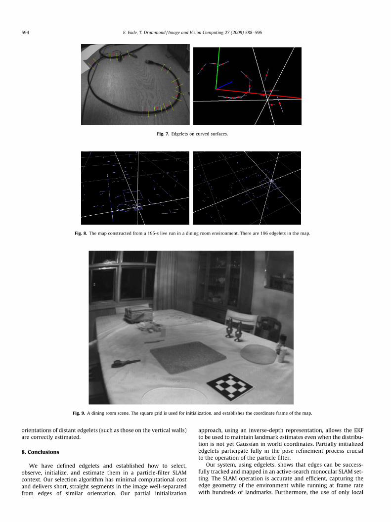
Fig. 7. Edgelets on curved surfaces.

Fig. 8. The map constructed from a 195-s live run in a dining room environment. There are 196 edgelets in the map.

Fig. 9. A dining room scene. The square grid is used for initialization, and establishes the coordinate frame of the map.

594 E. Eade, T. Drummond / Image and Vision Computing 27 (2009) 588–596

orientations of distant edgelets (such as those on the vertical walls)are correctly estimated.

8. Conclusions

We have defined edgelets and established how to select,observe, initialize, and estimate them in a particle-filter SLAMcontext. Our selection algorithm has minimal computational costand delivers short, straight segments in the image well-separatedfrom edges of similar orientation. Our partial initialization

approach, using an inverse-depth representation, allows the EKFto be used to maintain landmark estimates even when the distribu-tion is not yet Gaussian in world coordinates. Partially initializededgelets participate fully in the pose refinement process crucialto the operation of the particle filter.

Our system, using edgelets, shows that edges can be success-fully tracked and mapped in an active-search monocular SLAM set-ting. The SLAM operation is accurate and efficient, capturing theedge geometry of the environment while running at frame ratewith hundreds of landmarks. Furthermore, the use of only local

Fig. 10. The estimated trajectory of the camera in the dining room sequence. The trajectory is not post-processed; it represents the mode particle’s pose at the beginning ofeach time step.

E. Eade, T. Drummond / Image and Vision Computing 27 (2009) 588–596 595

portions of possibly extended edges yields a framework flexibleenough to map curved intensity changes.

While edge landmarks are useful for capturing higher-levelgeometry in scenes and when point features are scarce, they neednot be used in isolation. Future work should examine how pointsand edgelets can be used in tandem. Our current implementationalready permits this, but the difficulty lies in determining whenpoints rather than edges should be selected, and vice versa. A SLAMsystem might also wish group together individual landmarks(points and edgelets) into composite structures, to be estimatedas a group.

Appendix A. Edgelet observation model

All observations are first mapped into camera coordinates usingthe calibration parameters. In the following, R and T denote therotation matrix and the translation vector of the camera, respec-tively. These are parametrized as elements of SEð3Þ using the expo-nential map. A world point xW is mapped to the camera framecoordinates xC and then to the image plane coordinates ðu v ÞT by

xC ¼ RxW þ T ðA:1Þðu v ÞT ¼ projectðxCÞ ðA:2Þ

project

x

y

z

0B@

1CA � x=z

y=z

� �ðA:3Þ

A.1. Cartesian representation

The edgelet state is given as a 6-vector ðxT j dTÞT, with covari-ance P. The 3-vectors x and d are the center and direction of theedgelet in 3-space, respectively. The observation function yields acenter point xp and a direction dp in the image plane:

X � Rxþ T ðA:4ÞD � Rd ðA:5Þxp ¼ projectðXÞ ðA:6Þ

dp ¼X3D1 � X1D3

X3D2 � X2D3

� �ðA:7Þ

The linearizations needed for the EKF updates for pose and land-mark updates are as follows:

ðv�Þ �0 �v3 v2

v3 0 �v1

�v2 v1 0

0B@

1CA ðA:8Þ

oxp

oX¼ X�1

3

1 0 �X1X�13

0 1 �X2X�13

!ðA:9Þ

oxp

ox¼ oxp

oX

� �R ðA:10Þ

oxp

oT¼ oxp

oXðA:11Þ

oxp

oR¼ oxp

oX

� �ðX�Þ ðA:12Þ

odp

oX¼�D3 0 D1

0 �D3 D2

� �ðA:13Þ

odp

ox¼ odp

oX

� �R ðA:14Þ

odp

oD¼

X3 0 �X1

0 X3 �X2

� �ðA:15Þ

odp

od¼ odp

oD

� �R ðA:16Þ

odp

oT¼ odp

oXðA:17Þ

odp

oR¼ odp

oX

� �ðX�Þ þ

odp

oD

� �ðD�Þ ðA:18Þ

A.2. Inverse-depth representation

The partially initialized edgelet state is given as a 6-vectorðxT

q j dTqÞ

T, with covariance Pq, along with a fixed pose ðR0;T0Þ cor-responding to the initial view of the landmark. We refer to the vec-tors’ components:

xq � ðu v q ÞT ðA:19Þdq � ðdu dv dq ÞT ðA:20Þ

Components ðu; vÞ and ðdu;dvÞ correspond to the location and direc-tion, respectively, of the edgelet on the image plane in the initial

596 E. Eade, T. Drummond / Image and Vision Computing 27 (2009) 588–596

view. Component q describes the inverse depth of the edgelet in theinitial frame, and dq is its derivative. For a camera pose ðR;TÞ, thetransformation from the initial frame to the new frame is the resultof first transforming to world coordinates and then into the newpose:

R0 � R � RT0 ðA:21Þ

T0 � T� R0T0 ðA:22Þ

The observation model again maps the state to a center point anddirection in the image plane:

P � R0ðu v 1 ÞT þ q � T0 ðA:23ÞV � R0ðdu dv 0 ÞT þ dq � T0 ðA:24Þxp ¼ projectðPÞ ðA:25Þ

dp ¼P3V1 � P1V3

P3V2 � P2V3

� �ðA:26Þ

The Jacobians for the inverse-depth observation model are asfollows:

oxp

oP¼ P�1

3

1 0 �P1P�13

0 1 �P2P�13

!ðA:27Þ

ðA:28Þ

oxp

oT0¼ q � oxp

oPðA:29Þ

oxp

oR0¼ oxp

oP

� �ðP�Þ ðA:30Þ

odp

oP¼�V3 0 V1

0 �V3 V2

� �ðA:31Þ

ðA:32Þ

odp

oV¼

P3 0 �P1

0 P3 �P2

� �ðA:33Þ

ðA:34Þ

odp

oT0¼ q � odp

oPþ dq � odp

oVðA:35Þ

odp

oR0¼ðV1P2 � V2P1Þ 0 ðP2V3 � P3V2Þ

0 ðV1P2 � V2P1Þ ðP3V1 � P1V3Þ

� �ðA:36Þ

A.3. Intercept-slope form

Observations of edgelets are given in intercept-slope form rela-tive to a two-dimensional frame determined by an origin x0 and a

normal direction n in the image plane. The vector n acts as the y-axis in the intercept-slope equation y ¼ bþmx. The vectors x0 andn are determined in the landmark prediction phase from the modeparticle’s estimate. The two components of the observation arethen the parameters b and m, relative to x0 and n. The function thattakes xp and dp to intercept-slope form, and the corresponding Jac-obians, are as follows:

h � ð n1 �n0 ÞT ðA:37Þ

m ¼dT

pn

dTph

ðA:38Þ

b ¼ ðxp � x0ÞTn�m � ðxp � x0ÞTh ðA:39Þoboxp¼ n�m � h ðA:40Þ

ododp¼ n�m � h

dTph

ðA:41Þ

obodp¼ ðx0 � xpÞTh

ododp

ðA:42Þ

The innovation of an observation hypothesis (for use in the EKF)is then the difference between the observed intercept-slope andthe prediction, both relative to a fixed x0 and n.

References

[1] J.F. Canny, A computational approach to edge detection, in: IEEE Transactionson Pattern Analysis and Machine Intelligence, vol. 8, 1986.

[2] A. Davison, Real time simultaneous localisation and mapping with a singlecamera, in: ICCV, Nice, France, 2003.

[3] T. Drummond, R. Cipolla, Application of lie algebras to visual servoing, Int. J.Comput. Vis. 37 (1) (2000) 21–41.

[4] E. Eade, T. Drummond, Edge landmarks in monocular slam, in: Proceedings ofthe 17th British Machine Vision Conference, vol. 1, Edinburgh, 2006.

[5] E. Eade, T. Drummond, Scalable monocular slam, CVPR 1 (2006) 469–476.[6] J. Folkesson, P. Jensfelt, H. Christensen, Vision slam in the measurement

subspace, in: ICRA-05, IEEE, Barcelona, Spain, 2005.[7] A.P. Gee, W. Mayol-Cuevas, Real-time model-based slam using line segments,

in: 2nd International Symposium on Visual Computing, 2006. Available from:<http://www.cs.bris.ac.uk/Publications/Papers/2000570.pdf/>.

[8] M. Heath, S. Sarkar, T. Sanocki, K. Bowyer, Comparison of edge detectors: amethodology and initial study, in: CVPR’96, 1996.

[9] H. Jin, P. Favaro, S. Soatto, A semi-direct approach to structure from motion,Vis. Comput. 19 (6) (2003) 377–394.

[10] G. Klein, T. Drummond, A single-frame visual gyroscope, in: Proceedings of theBritish Machine Vision Conference (BMVC’05), vol. 2, BMVA, Oxford, 2005.

[11] N. Kwok, G. Dissanayake, Bearing-only slam in indoor environments using amodified particle filter, in: ACRA’03, 2003.

[12] T. Lemaire, S. Lacroix, Monocular-vision based SLAM using line segments, in:IEEE International Conference on Robotics and Automation, 2007.

[13] T. Lemaire, S. Lacroix, J. Sola, A practical 3d bearing-only slam algorithm, in:IROS 2005, 2005.

[14] M. Montemerlo, S. Thrun, D. Koller, B. Wegbreit, Fastslam 2.0: an improvedparticle filtering algorithm for simultaneous localization and mapping thatprovably converges, in: IJCAI, 2003.

[15] E. Rosten, T. Drummond, Fusing points and lines for high performancetracking, in: ICCV 2005, vol. 2, 2005.

[16] J.K.U.S.J. Julier, A new extension of the Kalman filter to nonlinear systems, in:The Proceedings of AeroSense, SPIE, Orlando, FL, USA, 1997.

[17] M.C. Shin, D. Goldgof, K.W. Bowyer, An objective comparison methodology ofedge detection algorithms using a structure from motion task, in: CVPR’98,IEEE Computer Society, Washington, DC, 1998.

[18] R. Sim, P. Elinas, M. Griffin, J.J. Little, Vision-based slam using the Rao-blackwellised particle filter, in: IJCAI Workshop on Reasoning withUncertainty in Robotics (RUR), Edinburgh, Scotland, 2005.

[19] P. Smith, I. Reid, A. Davison, Real-time monocular slam with straight lines, in:Proceedings of the 17th British Machine Vision Conference, vol. 1, Edinburgh,2006.

[20] C.J. Taylor, D.J. Kriegman, Structure and motion from line segments inmultiple images, IEEE Trans. Pattern Anal. Mach. Intell. 17 (11) (1995)1021–1032.