Embed Size (px)
Citation preview

Edexcel Level 3 Advanced GCE in Mathematics (9MA0)
Year 1 Scheme of Work
Term Time WK NO.
W/C Pure Statistics Mechanics
AU
TU
MN
TER
M 2
01
5
TER
M1
PA
RT1
Algebra and Functions Statistical Sampling
Data presentation and interpretation
Quantities and units in mechanics
1 06-Sep
Algebraic expressions- basic algebraic manipulation, indices and
surds
Introduction to sampling terminology; Advantages and
disadvantages of sampling Understand and use sampling
techniques; Compare sampling techniques in context
2 11-Sep Quadratic functions – factorising, solving, graphs and the discriminants
Calculation and interpretation of measures of location;
Calculation and interpretation of measures of variation;
Understand and use coding
3 18-Sep Equations – quadratic/linear simultaneous
4 25-Sep Inequalities – linear and quadratic (including graphical solutions)
5 02-Oct Graphs – cubic, quartic and reciprocal
Introduction to mathematical modelling and standard S.I. units of
length, time and mass
6 09-Oct Transformations – transforming graphs – f(x) notation
Definitions of force, velocity, speed, acceleration and weight and
displacement; Vector and scalar quantities

7 16-Oct
Coordinate geometry in the (x,y)
plane Further algebra
Data presentation and interpretation
Kinematics
TER
M 1
PA
RT
2
1 30-Oct Straight-line graphs,
parallel/perpendicular, length and area problems
Interpret diagrams for single-variable data; Interpret scatter diagrams and regression lines;
Recognise and interpret outliers; Draw simple
conclusions from statistical problems
2 06-Nov Circles – equation of a circle, geometric problems on a grid
3 13-Nov
4 20-Nov Algebraic division, factor theorem
and proof Graphical representation of velocity,
acceleration and displacement
5 27-Nov
6 04-Dec The binomial expansion Motion in a straight line under
constant acceleration; suvat formulae for constant acceleration;
Vertical motion under gravity 7 11-Dec
8 18-Dec
Trigonometry Vectors (2D)
Probability Statistical distributions
Forces & Newtons Laws
SPR
ING
TER
M
201
6
TER
M2
PA
RT1
1 03-Jan Trigonometric ratios and graphs (6
hours) Probability: Mutually exclusive events; Independent events (3
hours)
2 08-Jan
Statistical distributions: Use discrete distributions to model real-world situations; Identify

3 15-Jan
Trigonometric identities and equations (10 hours)
the discrete uniform distribution; Calculate
probabilities using the binomial distribution (calculator use
expected) (5 hours)
4 22-Jan
5 29-Jan
Definitions, magnitude/direction, addition and scalar multiplication
Newton’s first law, force diagrams, equilibrium, introduction to i, j
system (4 hours)
6 05-Feb
7 12-Feb Position vectors, distance between
two points, geometric problems
TER
M2
PA
RT2
Differentiation
Integration Statistical hypothesis testing Forces & Newton’s laws
1 26-Feb Definition, differentiating polynomials, second derivatives (6
hours)
Language of hypothesis testing; Significance levels (2 hours)
2 05-Mar
3 12-Mar Gradients, tangents, normals, maxima and minima (6 hours)
Carry out hypothesis tests involving the binomial distribution (5 hours)
4 19-Mar Definition as opposite of differentiation, indefinite integrals
of xn
Newton’s second law, ‘F = ma’, connected particles (no resolving forces or use of F = μR); Newton’s third law: equilibrium, problems
involving smooth pulleys (6 hours)
5 26-Mar
SUM
MER
TER
M 2
016
6 03-Apr
Definite integrals and areas under curves (5 hours)
Exponentials and logarithms Statistical Hypothesis testing Kinematics 2 (variable acceleration)
TER
M3
P
AR
T1
1 17-Apr Language of hypothesis testing;
Significance levels

2 23-Apr Exponentials and logarithms: Exponential functions and natural
logarithms
Revision Carry out hypothesis tests involving the binomial distribution
3 30-Apr Revision
4 07-May Revision Revision Variable force; Calculus to determine
rates of change for kinematics
5 14-May Revision Revision
6 21-May Revision Revision Use of integration for kinematics
problems i.e. d , dr v t v a t
TER
M3
PA
RT2
1 04-Jun Revision Revision Revision
2 11-Jun Revision Revision Revision
3 18-Jun Revision Revision Revision
4 25-Jun Revision Revision Revision
5 02-Jul Revision Revision Revision
6 09-Jul Revision Revision Revision
7 16-Jul Revision Revision Revision

Detailed Content Plan • Chapters 1 – 11 cover the pure mathematics content that is tested on AS paper 1 / A-level papers 1 & 2.
• Chapters 12 – 14 cover the statistics content that is tested on AS paper 2 / A-level paper 3.
• Chapters 15 – 16 cover the mechanics content that is tested on AS paper 2 / A-level paper 3.
This scheme of work is designed to accompany the use of Collins’ Edexcel A-level Mathematics Year 1 and AS Student Book, and references to sections in
that book are given for each lesson.
KEY
Ex – exercise
DS – Data set activity (Statistics chapters only)

Scheme of Work Edexcel A-level Mathematics Year 1 and AS (120 hours)
CHAPTER 1 – Algebra and functions 1: Manipulating algebraic expressions (8 Hours)
Prior knowledge needed GCSE Maths only
Technology Use the factorial and combinations button on a calculator.
One hour lessons Learning objectives Specification content Topic links Student Book
references
1 Manipulating polynomials algebraically
Students collect like terms with
expressions that include fractional
coefficients and are expected to write
expressions with terms written in
descending order of index. They expand a
single term over a bracket and expand
two binomials. They use the same
techniques to go on to expand three
simple binomials.
• Manipulate polynomials algebraically including: o expanding brackets and simplifying
by collecting like terms
AS Paper 1/A-level Papers 1 & 2: 1.1 – mathematical proof 2.6 – manipulate polynomials algebraically
Links back to GCSE 1.1 Ex 1.1A
2 Expanding multiple binomials
Students are introduced to Pascal’s
triangle and use this to expand multiple
binomials. One check students can use
when expanding multiple binomials is to
ensure the sum of the indices in each
term is the total of the index of the
original expansion. Students use factorial
• Understand and use the notation 𝑛! and 𝐶
𝑛𝑟
AS Paper 1/A-level Papers 1 & 2: 2.6 – manipulate polynomials algebraically 4.1 – binomial expansion
Links to Chapter 13 Probability and statistical distributions: 13.1 The binomial distribution
1.2 Ex 1.2A Ex 1.2B

notation when solve problems involving
combinations.
3 The binomial expansion
Students are introduced to the binomial
expansion formula as a way of solving any
binomial expansion, they should state
which formula they are using at the start
of any answer.
• Understand and use the binomial expansion of (𝑎 + 𝑏)𝑛
AS Paper 1/A-level Papers 1 & 2: 2.6 – manipulate polynomials algebraically 4.1 – binomial expansion
The binomial expansion is used in Chapter 13 Probability and statistical distributions for binomial distributions
1.3 Ex 1.3A
4 Factorisation
Students factorise different sorts of expressions including quadratics. They also factorise a difference of two squares. Some questions are given in relation to real life problems to show how factorisation is used.
• Manipulate polynomials algebraically including: o factorisation
AS Paper 1/A-level Papers 1 & 2: 2.6 – manipulate polynomials algebraically
Factorisation is used in Chapter 2 Algebra and functions 2: Equations and inequalities when working with quadratic equations and in Chapter 3 Algebra and functions 3: Sketching curves
1.4 Ex 1.4A
5 Algebraic division All the skills are then combined to write algebraic fractions in their simplest form. Students work through the factor theorem. Students then divide polynomials by an expression – make it clear to students that they use the same method as they do for numerical long division.
• Manipulate polynomials algebraically including: o expanding brackets and simplifying
by collecting like terms o factorisation o simple algebraic division o use of the factor theorem
AS Paper 1/A-level Papers 1 & 2: 2.6 – manipulate polynomials algebraically, including expanding brackets, collecting like terms, factorisation and simple algebraic division; use of the factor theorem
Link algebraic division to numerical division
1.5 Ex 1.5A
6 Laws of indices, manipulating surds Students solve questions using the laws of indices, including negative and fractional
• Understand and use the laws of indices for all rational exponents
• Use and manipulate surds
AS Paper 1/A-level Papers 1 & 2: 1.1 – mathematical proof
Builds on GCSE skills Laws of indices is used in Chapter 7 Exponentials and logarithms, section 7.2
1.6 1.7 Ex 1.6A Ex 1.7A

indexes. They are reminded that surds are roots of rational numbers and simplify expressions involving surds.
2.1 – understand and use the laws of indices for all rational exponents 2.2 - use and manipulate surds, including rationalising the denominator
Manipulation of indices and surds is used in Chapter 8 Differentiation and Chapter 9 Integration
7 Rationalising the denominator Recap manipulating surds and complete Ex 1.7A if required and then students go on to rationalise the denominator of algebraic fractions.
• Use and manipulate surds, including rationalising the denominator
AS Paper 1/A-level Papers 1 & 2: 1.1 – mathematical proof 2.2 - use and manipulate surds, including rationalising the denominator
1.8 Ex 1.8A
8 Chapter review lesson Recap key points of chapter. Students to complete the exam-style questions, extension questions, or online end-of-chapter test
• Identify areas of strength and development within the content of the chapter
See below
Assessment Exam-style questions 1 in Student Book Exam-style extension questions 1 in Student Book End-of-chapter test 1 on Collins Connect
CHAPTER 2 – Algebra and functions 2: Equations and inequalities (8 Hours)
Prior knowledge needed Chapter 1
Technology Use a calculator to check solutions to quadratic equations that have been solved by hand. Use a graphing software to plot lines when solving simultaneous equations so that students can see that where the lines intersect is the solution. Use graphing software to show the solutions to quadratic inequalities.
One hour lessons Learning objectives Specification content Topic links Student Book
references

1 Quadratic functions
Students draw and work out key aspects
of quadratic functions, they also work out
equations of given quadratic graphs.
Make students aware that the notation
f(x) may be used.
Consider the difference between drawing
and sketching.
• Work with quadratic functions and their graphs
AS Paper 1/A-level Papers 1 & 2: 2.3 – work with quadratics functions and their graphs
Make connections back to factorising in 1.4 Factorisation
2.1 Ex 2.1A
2 The discriminant of a quadratic
function
Students are reminded that the
discriminant is 𝑏2– 4𝑎𝑐 and that the value
of the discriminant indicates what type of
roots and number of solutions a quadratic
has. Link this to how students will sketch
quadratics in the next chapter. Students
need to make sure they have a quadratic
in the form 𝑎𝑥2 + 𝑏𝑥 + 𝑐 = 0 before they
calculate the discriminant.
• Calculate and use the discriminant of a quadratic function, including the conditions for real and repeated roots
AS Paper 1/A-level Papers 1 & 2: 2.3 – work with the discriminant of a quadratic function, including the conditions for real and repeated roots
Links to 3.1 Sketching curves of quadratic functions
2.2 Ex 2.2A
3 Completing the square
Students complete the square on the
general expression of a quadratic. They go
onto solving quadratic equations by
completing the square.
The general formula for solving a
quadratic equation can be derived by
completing the square on the general
form 𝑦 = 𝑎𝑥2 + 𝑏𝑥 + 𝑐 – this is question
6 in Ex 2.4A.
• Complete the square AS Paper 1/A-level Papers 1 & 2: 1.1 – mathematical proof 2.3 – complete the square
5.1 Equations of circles uses completing the square when solving problems involving circles Links to 3.1 sketching curves of quadratic functions
2.3 Ex 2.3A

4 Solving quadratic equations Students use factorisation, using the formula, completing the square and calculators to solve quadratic equations, they consider advantages and disadvantages of each method. It’s important not to be seen as a discrete set of skills but providing different information about the same equation.
• Solve quadratic equations using o completing the square o the formula o factorisation
AS Paper 1/A-level Papers 1 & 2: 1.1 – mathematical proof 2.3 – solve quadratic equations
The ability to find solutions will help you solve distance, speed and time problems in Chapter 15 Kinematics and in Chapter 6 Trigonometry and Chapter 7 Exponentials and logarithms Link to graph drawing, 3.1 Sketching curves of quadratic functions
2.4 Ex 2.4A
5 Solving simultaneous equations Students go through solving two linear simultaneous equations by elimination and then by substitution. They need to think about which is the best method and why.
• Solve simultaneous equations in two variables by o elimination or o by substitution, including one linear and one quadratic equation
AS Paper 1/A-level Papers 1 & 2: 2.4 – solve simultaneous equations in two variables by elimination and by substitution, including one linear and one quadratic equation
This is used when finding points of intersection with circles and straight lines in Chapter 5 Coordinate geometry 2: Circles
2.5 Ex 2.5A Ex 2.5B
6 Solving linear and quadratic simultaneous equations Student solve linear and quadratic simultaneous equations considering which method is the most appropriate to use.
• Solve simultaneous equations in two variables by o elimination or o by substitution, including one linear and one quadratic equation
AS Paper 1/A-level Papers 1 & 2: 2.4 – solve simultaneous equations in two variables by elimination and by substitution, including one linear and one quadratic equation
2.6 Ex 2.6A
7 Solving linear and quadratic inequalities Students solve inequalities, use set notation to list integer members of two or more combined inequalities and represent inequalities graphically. Strict inequalities are represented with a dotted line, inclusive inequalities are represented with a solid line.
• Solve linear and quadratic inequalities in a single variable and interpret such inequalities graphically, including inequalities with brackets and fractions
• Express solutions through correct use of ‘and’ and ‘or’, or through set notation
AS Paper 1/A-level Papers 1 & 2: 2.5 - solve linear and quadratic inequalities in a single variable and interpret such inequalities graphically, including inequalities with brackets and fractions 2.5 - express solutions through correct use of ‘and’ and ‘or’, or through set notation
This is used in Chapter 5 Coordinate geometry 2: Circles when solving problems involving equations of circles
2.7 Ex 2.7A 2.8 Ex 2.8A

Link to solving equations, drawing graphs and looking at inequalities from the sketch of a graph.
8 Chapter review lesson Recap key points of chapter. Students to complete the exam-style questions, extension questions, or online end-of-chapter test
• Identify areas of strength and development within the content of the chapter
See below
Assessment Exam-style questions 2 in Student Book Exam-style extension questions 2 in Student Book End-of-chapter test 2 on Collins Connect
CHAPTER 3 – Algebra and functions 3: Sketching curves (9 Hours)
Prior knowledge needed Chapter 2
Technology Graphing software can be heavily used in this chapter; some examples are below. Use graphing software to check answers. Use graphing software to zoom into a point of inflection and see what happens to the gradient of the curve each side of the point of inflection. Use graphing software to compare how to graphs behave. Use graphing software to look at approximate coordinates of turning points.
One hour lessons Learning objectives Specification content Topic links Student Book
references
1 Sketching curves of quadratic functions
Students sketch curves of quadratic
equations and find quadratic equations
from sketches knowing that a sketch
shows the curve along with its key
features. The key features being;
maximum or minimum turning point and
• Use and understand the graphs of functions
• Sketch curves defined by simple quadratic equations
AS Paper 1/A-level Papers 1 & 2: 2.3 – work with quadratic functions and their graphs 2.7 – understand and use graphs of functions; sketch curves defined by simple equations
Builds on from Chapter 2 Algebra and functions 2: Equations and inequalities
3.1 Ex 3.1A

its coordinates, the roots with x
intercept/s if appropriate, the y intercept.
2 Sketching curves of cubic functions
Students consider how the cubic functions
behaves as it tends to positive and
negative infinity, this determines the
shape of the curve. The coordinates of the
axes intercepts and point of inflection are
included on the graph. Students use this
information to sketch curves of cubic
functions.
• Use and understand the graphs of functions
• Sketch curves defined by simple cubic equations
AS Paper 1/A-level Papers 1 & 2: 2.7 - understand and use graphs of functions; sketch curves defined by simple equations 2.7 – interpret algebraic solutions of equations graphically
Builds on from Chapter 2 Algebra and functions 2: Equations and inequalities
3.2 Ex 3.2A Ex 3.2B
3 Sketching curves of quartic functions
Students find turning points and points of
intersection to sketch curves of quartic
functions. They look at maximum and
minimum turning points and then at the
roots of the equation. A typical example
of a quartic to be sketched is = 𝑥2(2𝑥 −
1)2 .
• Use and understand the graphs of functions
• Sketch curves defined by simple quartic equations
• Interpret the algebraic solution of equations graphically
AS Paper 1/A-level Papers 1 & 2: 2.7 - understand and use graphs of functions; sketch curves defined by simple equations 2.7 – interpret algebraic solutions of equations graphically
Builds on from Chapter 2 Algebra and function 2: Equations and inequalities
3.3 Ex 3.3A Ex 3.3B
4 Sketching curves of reciprocal functions Students sketch graphs of reciprocals of
linear 𝑦 =𝑎
𝑥 and quadratic 𝑦 =
𝑎
𝑥2
functions. They are introduced to the word discontinuity and know that this is a point where the value of x or y is not defined. They also are told that an asymptote is a straight line that a curve approaches but never meets, these should
• Use and understand the graphs of functions
• Sketch curves defined by simple reciprocals
• Interpret the algebraic solution of equations graphically
AS Paper 1/A-level Papers 1 & 2: 2.7 - understand and use graphs of functions; sketch curves defined by simple equations
including polynomials 𝑦 =𝑎
𝑥 and
𝑦 =𝑎
𝑥2 (including their vertical
and horizontal asymptotes)
Graph sketching skills are further developed in Chapter 7 Exponentials and logarithms
3.4 Ex 3.4A Ex 3.4B

be clearly highlighted on the graph. They also give the points of interception on the axis.
5 Intersection points Students sketch more than one function on a graph to work out the intersection points of the functions and link this to solve an equation which includes these functions. They use the information they have learnt for the previous section in this exercise to solve these problems.
• Use intersection points of graphs to solve equations
AS Paper 1/A-level Papers 1 & 2: 2.7 interpret algebraic solution of equations graphically; use intersection points of graphs to solve problems
Links back to 2.5 Solving simultaneous equations
3.5 Ex 3.5A
6 Proportional relationships Students express the relationship between two variables using the proportion symbol and then find the equation between the two variables. They also recognise and use graphs that show proportion.
• Understand and use proportional relationships and their graphs
AS Paper 1/A-level Papers 1 & 2: 2.7 – understand and use proportional relationships and their graphs
Links back to GCSE 3.6 Ex 3.6A
7 Translations Students transform functions and sketch the resulting graphs using the two transformations identified in the learning objective.
• Understand the effects of simple transformations on the graphs of 𝑦 = f(𝑥), including 𝑦 = f(𝑥) + 𝑎 and 𝑦 = f(𝑥 + 𝑎)
AS Paper 1: 2.8 – effects of simple transformations including sketching associated graphs A-level Papers 1 & 2: 2.9 – effects of simple transformations including sketching associated graphs
Translations and stretches arise in 6.5 solving trigonometric equations
3.7 Ex 3.7A
8 Stretches Students transform functions and sketch the resulting graphs using the two transformations identified in the learning objective.
• Understand the effects of simple transformations on the graphs of 𝑦 = f(𝑥), including 𝑦 = 𝑎f(𝑥) and 𝑦 = f(𝑎𝑥).
AS Paper 1: 2.8 – effects of simple transformations including sketching associated graphs# A-level Papers 1 & 2:
Translations and stretches arise in 6.5 solving trigonometric equations
3.8 Ex 3.8A

2.9 – effects of simple transformations including sketching associated graphs
9 Chapter review lesson Recap key points of chapter. Students to complete the exam-style questions, extension questions, or online end-of-chapter test
• Identify areas of strength and development within the content of the chapter
See below
Assessment Exam-style questions 3 in Student Book Exam-style extension questions 3 in Student Book End-of-chapter test 3 on Collins Connect
CHAPTER 4 – Coordinate geometry 1: Equations of straight lines (5 Hours)
Prior knowledge needed Chapter 1
Technology Use graphing software to check answers. Use graphing software to investigate the location of the x-intercept as the gradient varies with both positive and negative and integer and fractional values. Use graphing software to find equations of lines that are parallel. Use graphing software to plot lines that intersect but are not perpendicular. What do the students notice about the products of their gradients?
One hour lessons Learning objectives Specification content Topic links Student Book
references
1 Straight line graphs – part 1
Students rearrange equations of straight
lines to the form 𝑎𝑥 + 𝑏𝑦 + 𝑐 = 0
Students find the equation of a line given
the gradient and a point on the line and
solve problems using this.
• Write the equation of a straight line in the form 𝑎𝑥 + 𝑏𝑦 + 𝑐 = 0
• Find the equation of a straight line through one point with a given gradient using the formula 𝑦– 𝑦1 = 𝑚(𝑥– 𝑥1)
AS Paper 1/A-level Papers 1 & 2: 3.1 – understand and use the equation of a straight line, including the forms 𝑦– 𝑦1 = 𝑚(𝑥– 𝑥1) and 𝑎𝑥 + 𝑏𝑦 + 𝑐 = 0
4.2 and 4.3 link to Chapter 15 Kinematics
4.1 Ex 4.1A 4.2 Ex 4.2A

2 Straight line graphs – part 2 Students find the gradient given two points on the line and solve problems using this. Given two points on a line students use the formula to find the equation of the straight line.
• Find the gradient of the straight line between two points
• Find the equation of a straight line
using the formula 𝑦–𝑦1
𝑦2–𝑦1=
𝑥–𝑥1
𝑥2–𝑥1
AS Paper 1/A-level Papers 1 & 2: 3.1 – understand and use the equation of a straight line, including the forms 𝑦– 𝑦1 = 𝑚(𝑥– 𝑥1) and 𝑎𝑥 + 𝑏𝑦 + 𝑐 = 0
Graph sketching skills are further developed in Chapter 7 Exponentials and logarithms
4.3 Ex 4.3A 4.4 Ex 4.4A
3 Parallel and perpendicular lines Students use the facts about gradients of parallel and perpendicular straight lines to solve problems.
• Understand and use the gradient conditions for parallel lines
• Understand and use the gradient conditions for perpendicular lines
AS Paper 1/A-level Papers 1 & 2: 3.1 – gradient conditions for two straight lines to be parallel or perpendicular
Links back to GCSE 4.5 Ex 4.5A Ex 4.5B
4 Straight line models Students apply what they have learnt in this chapter to solve problems in a variety of different contexts including real-world scenarios.
• Be able to use straight line models in a variety of contexts
AS Paper 1/A-level Papers 1 & 2: 3.1 – be able to use straight line models in a variety of contexts
This is used in Chapter 5 Coordinate geometry 2: Circles when finding a gradient to solve problems involving tangents and radii of circles and points of intersections of circles with straight lines
4.6 Ex 4.6A
5 Chapter review lesson Recap key points of chapter. Students to complete the exam-style questions, extension questions, or online end-of-chapter test
• Identify areas of strength and development within the content of the chapter
See below
Assessment Exam-style questions 4 in Student Book Exam-style extension questions 4 in Student Book End-of-chapter test 4 on Collins Connect

CHAPTER 5 – Coordinate geometry 2: Circles (6 Hours)
Prior knowledge needed Chapter 2 Chapter 4
Technology Use graphing software draw 𝑥2 + 𝑦2 = 25 and 𝑥2 + 𝑦2 = 36 to show how the centre of a circle is always (0, 0) and the radius is the square root of the number on the right-hand side of the equation. Get students to predict what other circles will look like given an equation of a circle in this form. Graphing software can be used to look at other circles (still with the equation written in this form but not with centre (0, 0) ) and link the equation of the circle to the coordinates of the centre and length of radius. Use graphing software to find midpoints of line segments. Use graphing software to plot a circle and tangent.
One hour lessons Learning objectives Specification content Topic links Student Book
references
1 Equations of circles – part 1
Students link equations of circles to
Pythagoras’ theorem. They learn the
general equation of a circle and solve
problems. They find the equation of a
circle from its centre and a point on the
circumference. Given an equation of a
circle students find the centre and radius
by completing the square on 𝑥 and 𝑦.
• Find the centre of the circle and the radius from the equation of a circle
• Write the equation of a circle
AS Paper 1/A-level Papers 1 & 2: 3.2 – understand and use the coordinate geometry of the circle including using the equation of a circle in the form (𝑥– 𝑎)2 + (𝑦– 𝑏)2 = 𝑟2 3.2 – complete the square to find the centre and radius of a circle
Links back to GCSE 5.1 Ex 5.1A
2 Equations of circles – part 2
Recap lesson one and then students find
the equation of a circle from the ends of a
diameter, this involves them using the
formula for the midpoint of a line
segment.
• Find the centre of the circle and the radius from the equation of a circle
• Write the equation of a circle
AS Paper 1/A-level Papers 1 & 2: 3.2 – understand and use the coordinate geometry of the circle including using the equation of a circle in the form (𝑥– 𝑎)2 + (𝑦– 𝑏)2 = 𝑟2 3.2 – complete the square to find the centre and radius of a circle
5.1 Ex 5.1B

3 Angles in semicircles
A geometric proof is used to show that for
three points on the circumference of a
circle, if two points are on a diameter,
then the triangle is right-angled. Students
are also reminded that Pythagoras’
theorem will show that a triangle has a
right angle and gradients can be used to
show that two lines are perpendicular.
• Find the equation of a circle given different information such as the end points of a diameter
• Use circle theorems to solve problems
AS Paper 1/A-level Papers 1 & 2: 1.1 - mathematical proof 3.2 - use of the following properties: the angle in a semicircle is a right angle
Links back to GCSE 5.2 Ex 5.2A
4 Perpendicular from the centre to a
chord
A geometric proof is used to show that
congruent triangles are identical and then
links to show that the perpendicular from
the centre of the circle to a chord bisects
the chord.
• Find the equation of a perpendicular bisector
• Use circle theorems to solve problems
AS Paper 1/A-level Papers 1 & 2:
3.2 - use of the following
properties: the perpendicular from the centre to a chord bisects to chord
Links back to GCSE 5.3 Ex 5.3A
5 Radius perpendicular to the tangent A geometric proof by contradiction is used to show that a radius and tangent are perpendicular at the point of contact. Pythagoras’ theorem is used to find the length of a tangent. Students then go on to consider that for any circle there are two tangents with the same gradient. Given the gradient of the tangent and the equation of the circle they can find both points where the two tangents touch the circle. The second method used it to show that a line is tangent to a circle is that the discriminant will be zero i.e. 𝑏2– 4𝑎𝑐 = 0.
• Find the equation and length of a tangent
• Use circle theorems to solve problems
AS Paper 1/A-level Papers 1 & 2:
3.2 - use of the following
properties: the radius of a circle at a given point on its circumference is perpendicular to the tangent to the circle at that point
5.4 Ex 5.4A Ex 5.4B
6 Chapter review lesson Recap key points of chapter. Students to complete the exam-style questions, extension questions, or online end-of-chapter test
• Identify areas of strength and development within the content of the chapter
See below
Assessment Exam-style questions 5 in Student Book Exam-style extension questions 5 in Student Book End-of-chapter test 5 on Collins Connect
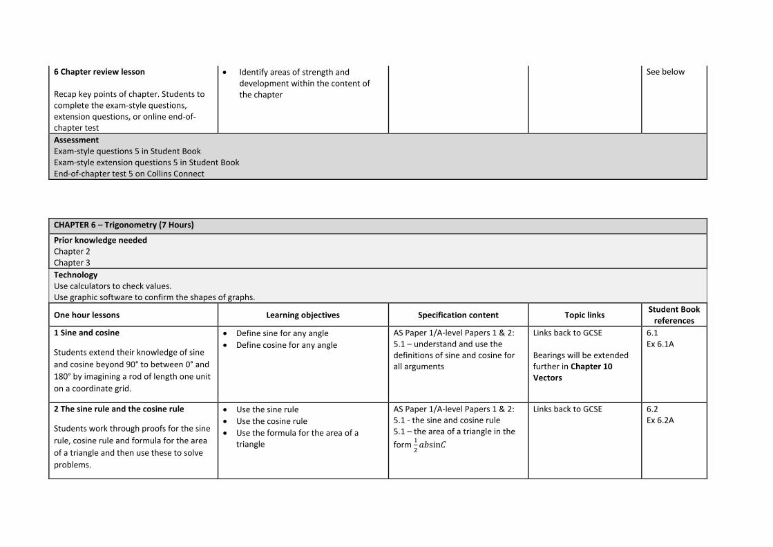
CHAPTER 6 – Trigonometry (7 Hours)
Prior knowledge needed Chapter 2 Chapter 3
Technology Use calculators to check values. Use graphic software to confirm the shapes of graphs.
One hour lessons Learning objectives Specification content Topic links Student Book
references
1 Sine and cosine
Students extend their knowledge of sine
and cosine beyond 90° to between 0° and
180° by imagining a rod of length one unit
on a coordinate grid.
• Define sine for any angle
• Define cosine for any angle
AS Paper 1/A-level Papers 1 & 2: 5.1 – understand and use the definitions of sine and cosine for all arguments
Links back to GCSE Bearings will be extended further in Chapter 10 Vectors
6.1 Ex 6.1A
2 The sine rule and the cosine rule
Students work through proofs for the sine
rule, cosine rule and formula for the area
of a triangle and then use these to solve
problems.
• Use the sine rule
• Use the cosine rule
• Use the formula for the area of a triangle
AS Paper 1/A-level Papers 1 & 2: 5.1 - the sine and cosine rule 5.1 – the area of a triangle in the
form 1
2𝑎𝑏sin𝐶
Links back to GCSE 6.2 Ex 6.2A

3 Trigonometric graphs
Students start by considering the sine and
cosine of any angle using x and y
coordinates of points on the unit circle.
This is then linked to the trigonometric
graphs and their symmetries and
periodicity.
• Understand the graph of the sine function and interpret its symmetry and periodicity
• Understand the graph of the cosine function and interpret its symmetry and periodicity
AS Paper 1: 5.2 – Understand and use the sine and cosine functions; their graphs, symmetries and periodicity A-level Papers 1 & 2: 5.3 – Understand and use the sine and cosine functions; their graphs, symmetries and periodicity
Link back to GCSE 6.3 Ex 6.3A
4 The tangent function Students consider when the tangent cannot be calculated and look at the similarities between the tangent graph and the sine and cosine graphs. They use
tanƟ =sinƟ
cosƟ to solve problems.
• Define the tangent for any angle
• Understand the graph of the tangent function and interpret its symmetry and periodicity
• Use an important formula connecting sin 𝑥, cos 𝑥 and tan 𝑥
AS Paper 1: 5.1 – understand and use the definition of tangent for all arguments 5.2 - Understand and use the tangent functions; its graph, symmetry and periodicity 5.3 – understand and use
tanƟ =sinƟ
cosƟ
A-level Papers 1 & 2: 5.1 – understand and use the definition of tangent for all arguments 5.3 - Understand and use the tangent functions; its graph, symmetry and periodicity 5.5 – understand and use
tanƟ =sinƟ
cosƟ
Link to Chapter 4 Coordinate geometry 1: Equations of straight lines
6.4 Ex 6.4A
5 Solving trigonometric equations Students thing about the multiple solutions of trigonometric equations and link this to the graphs of the function.
• Solve simple trigonometric equations AS Paper 1: 5.4 – solve simple trigonometric equations in a given interval, including quadratic equations in sin, cos and tan and equations involving multiples of the unknown angle
Link this back to transformation of graphs in Chapter 3 Algebra and functions 3
6.5 Ex 6.5A

A-level Papers 1 & 2: 5.7 – solve simple trigonometric equations in a given interval, including quadratic equations in sin, cos and tan and equations involving multiples of the unknown angle
6 A useful formula Students diagrammatically see that sin2Ɵ + cos2Ɵ = 1 and then use this identity to go on to solve trigonometric equations. Link to Pythagoras’ theorem.
• Use an important formula connecting sin 𝑥, cos 𝑥 and tan 𝑥
AS Paper 1: 5.3 – understand and use sin2Ɵ +cos2Ɵ = 1 A-level Papers 1 & 2: 5.5 – understand and use sin2Ɵ +cos2Ɵ = 1
Link to Pythagoras’ theorem.
6.6 Ex 6.6A
7 Chapter review lesson Recap key points of chapter. Students to complete the exam-style questions, extension questions, or online end-of-chapter test
• Identify areas of strength and development within the content of the chapter
See below
Assessment Exam-style questions 6 in Student Book Exam-style extension questions 6 in Student Book End-of-chapter test 6 on Collins Connect
CHAPTER 7 – Exponentials and logarithms (8 Hours)
Prior knowledge needed Chapter 1 Chapter 2

Chapter 3 Chapter 4
Technology Graph plotting software to draw the graphs 𝑦 = 1.2𝑥. Use the log, power of e and ln button on a calculator. Use spreadsheet software to calculate values of logarithms.
One hour lessons Learning objectives Specification content Topic links Student Book
references
1 The function 𝒂𝒙
Students learn the terms exponential
growth and exponential decay. The draw
graphs of the form 𝑦 = 𝑎𝑥 and are made
aware that there is a difference in the
shape of the graph when a < 1 and a > 1,
they should understand this.
• Use and manipulate expressions in the form 𝑦 = 𝑎𝑥 where the variable x is an index
• Draw and interpret graphs of the form 𝑦 = 𝑎𝑥
• Use the graph to find approximate solutions
AS Paper 1/A-level Papers 1 & 2: 6.1 – Know and use the function 𝑎𝑥 and its graph, where a is positive
Links back to GCSE 7.1 Ex 7.1A
2 Logarithms
Students start with the laws of logarithms
in base 10 and the laws of logarithms are
linked to laws of indices with a proof for
each law. They work out basic logarithms
in base 10 without a calculator. They then
move onto using the laws for logarithms
of any base and using the log𝑎𝑏 button on
a calculator.
• Understand and use logarithms and their connection with indices
• Understand the proof of the laws of logarithms
AS Paper 1/A-level Papers 1 & 2: 6.3 – know and use the definition of log𝑎𝑥 as the inverse of 𝑎𝑥, where 𝑎 is positive and 𝑥 ≥ 0 6.4 – understand and use the laws of logarithms
The skills learnt in 1.6 Laws of indices are used here
7.2 Ex 7.2A Ex 7.2B
3 The equation 𝒂𝒙 = 𝒃
Students solve equations of the form
𝒂𝒙 = 𝒃 by taking the logarithms of both
sides. The work through a proof of the
• Solve equations in the form 𝑎𝑥 = 𝑏
• Understand a proof of the formula to change the base of a logarithm
AS Paper 1/A-level Papers 1 & 2: 6.5 – solve equations in the form 𝑎𝑥 = 𝑏
7.3 Ex 7.3A

formula to change the base of a
logarithm.
4 Logarithmic graphs Students look at two different types of curve 𝑦 = 𝑎𝑥𝑛 and 𝑦 = 𝑘𝑏𝑥. To find the parameters they take the logarithms of both sides and then rearrange this equation into the form 𝑦 = 𝑚𝑥 + 𝑐. In the first case they plot log 𝑦 against log 𝑥 and obtain a straight line where the intercept is log 𝑎 and the gradient is 𝑛 and in the second case they plot log 𝑦 against 𝑥 and obtain a straight line where the intercept is log 𝑘 and the gradient is log 𝑏.
• Use and manipulate expressions in the form 𝑦 = 𝑘𝑎𝑥 where the variable x is an index
• Use logarithmic graphs to estimate parameters in relationships of the form 𝑦 = 𝑎𝑥𝑛 and 𝑦 = 𝑘𝑏𝑥, given data for 𝑥 and 𝑦
AS Paper 1/A-level Papers 1 & 2: 6.3 – know and use the definition of log𝑎𝑥 as the inverse of 𝑎𝑥, where 𝑎 is positive and 𝑥 ≥ 0 6.6 – use logarithmic graphs to estimate parameters in relationships of the form 𝑦 = 𝑎𝑥𝑛 and 𝑦 = 𝑘𝑏𝑥, given data for 𝑥 and 𝑦
7.4 Ex 7.4A
5 The number e Students look at graphs of the form 𝑦 = 𝑎𝑥 . and see the gradient is always a multiplier x 𝑦. When the multiplier is one then the function is of the form 𝑦 = 𝑒𝑥 and go on to generalise that for 𝑦 = 𝑒𝑎𝑥 then the gradient = 𝑎𝑒𝑎𝑥 = 𝑎𝑦 for any value of 𝑎. Students should realise that when the rate of change is proportional to the 𝑦 value, an exponential model should be used. Insure that students include the graphs of 𝑦 = 𝑒𝑎𝑥 + 𝑏 + 𝑐.
• Know that the gradient of 𝑒𝑘𝑥 is equal
to 𝑘𝑒𝑘𝑥 and hence understand why the exponential model is suitable in many applications
AS Paper 1/A-level Papers 1 & 2: 6.1 – Know and use the function 𝑒𝑥 and its graph 6.2 – Know that the gradient of
𝑒𝑘𝑥 is equal to 𝑘𝑒𝑘𝑥 and hence understand why the exponential model is suitable in many applications
7.5 Ex 7.5A
6 Natural logarithms Students are introduced to the fact that ln𝑦 means logarithm to the base 𝑒 and that if 𝑒𝑥 = 𝑦 then ln𝑦 = 𝑥. The graphs of
• Know and use the function ln𝑥 and its graphs
• Know and use ln𝑥 as the inverse function of 𝑒𝑥
AS Paper 1/A-level Papers 1 & 2: 6.3 – know and use the function ln𝑥 and its graph 6.3 – know and use ln𝑥 as the inverse function of 𝑒𝑥
7.6 Ex 7.6A
𝑦 = ln𝑥 and 𝑦 = 𝑒𝑥 show students that they are a reflection of each other in the line 𝑦 = 𝑥 due to the fact they are inverse function. Solutions of equations of the
form 𝑒𝑎𝑥+𝑏 = 𝑝 and ln(𝑎𝑥 + 𝑏) = 𝑞 is expected.
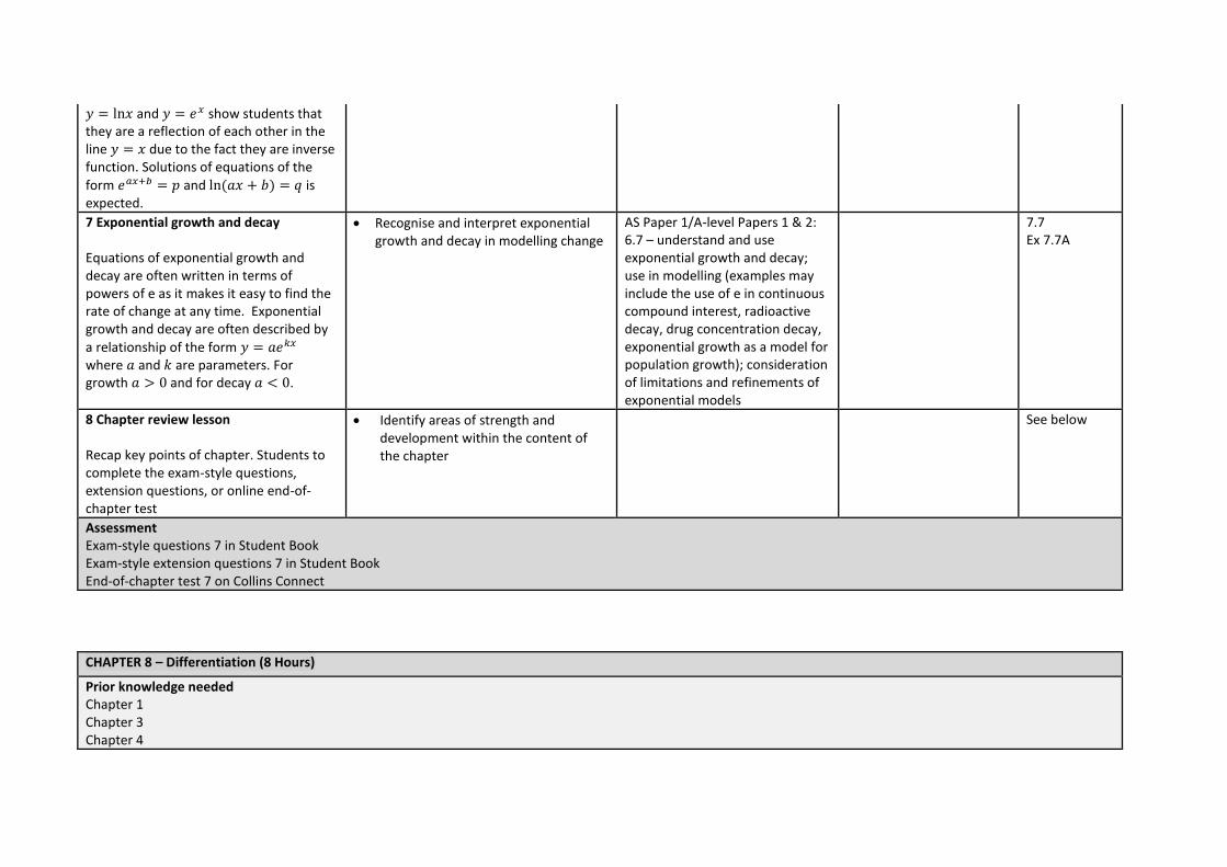
7 Exponential growth and decay Equations of exponential growth and decay are often written in terms of powers of e as it makes it easy to find the rate of change at any time. Exponential growth and decay are often described by
a relationship of the form 𝑦 = 𝑎𝑒𝑘𝑥 where 𝑎 and 𝑘 are parameters. For growth 𝑎 > 0 and for decay 𝑎 < 0.
• Recognise and interpret exponential growth and decay in modelling change
AS Paper 1/A-level Papers 1 & 2: 6.7 – understand and use exponential growth and decay; use in modelling (examples may include the use of e in continuous compound interest, radioactive decay, drug concentration decay, exponential growth as a model for population growth); consideration of limitations and refinements of exponential models
7.7 Ex 7.7A
8 Chapter review lesson Recap key points of chapter. Students to complete the exam-style questions, extension questions, or online end-of-chapter test
• Identify areas of strength and development within the content of the chapter
See below
Assessment Exam-style questions 7 in Student Book Exam-style extension questions 7 in Student Book End-of-chapter test 7 on Collins Connect
CHAPTER 8 – Differentiation (8 Hours)
Prior knowledge needed Chapter 1 Chapter 3 Chapter 4

Technology Use graphical software to find the gradients of a quadratic curve in example 2 in section 8.2. Graphical software can be used to look for stationary points – students also need to find them using differentiation.
One hour lessons Learning objectives Specification content Topic links Student Book
references
1 The gradient of a curve
Students are introduced to the concept
that the gradient of a curve at any point is
equal to the gradient of the tangent at
that point.
Students then look at 𝑦 = 𝑥2 and see that
the gradient at any point on the curve is
2𝑥. The derivative is then introduced as
the connection between the x coordinate
of a point and the gradient of the curve at
that point.
• To consider the relationship between the tangent to a curve and the gradient of the curve at a point
• Introduction of the term derivative
• Recognise the derivative function of 𝑦 = 𝑥2
AS Paper 1/A-level Papers 1 & 2: 7.1 – understand and use the derivative of f(𝑥) as the gradient of the tangent to a graph of 𝑦 =f(𝑥) at a general point (𝑥, 𝑦); the gradient of the tangent as a limit; interpretation as a rate of change
The skills learnt in this chapter are essential when students learn Chapter 9 Integration
8.1 Ex 8.1A 8.2 Ex 8.2A
2 The gradient of a quadratic curve
From exercise 8.2A students are lead to the general result that if 𝑦 = 𝑎𝑥2 then 𝑑𝑦
𝑑𝑥= 2𝑎𝑥. After some examples students
are given the general result when differentiating a quadratic. It is also made clear that terms should be differentiated separately in a quadratic equation. They start to sketch curves of the derivative.
• Extend the result for the derivative of 𝑦 = 𝑥2 to the general case 𝑦 = 𝑎𝑥2
• Be able to differentiate any quadratic equation
AS Paper 1/A-level Papers 1 & 2: 7.1 – sketching the gradient function for a given curve 7.2 – differentiate 𝑥𝑛, for rational values of 𝑛, and related constant multiples, sums and differences
8.2 Ex 8.2B
3 Differentiation of 𝒙𝟐 and 𝒙𝟑
Students work through a proof that the
derivative of 𝑥2 is 2𝑥, they are told that
using the formula is called differentiation
from first principles.
• Understand a proof that if 𝑓(𝑥) = 𝑥2 then 𝑓’(𝑥) = 2𝑥
AS Paper 1/A-level Papers 1 & 2: 7.1 – differentiation from first principals for small positive integer powers of 𝑥 7.2 - differentiate 𝑥𝑛, for rational values of 𝑛, and related constant multiples, sums and differences
8.3 Ex 8.3A

4 Differentiation of a polynomial The general result for differentiation is introduced to students and examples are worked through. They then go on to looking at differentiating the sum or difference of terms.
• Differentiate expressions containing integer powers
AS Paper 1: A-level Papers 1 & 2: 7.2 - differentiate 𝑥𝑛, for rational values of 𝑛 , and related constant multiples, sums and differences
8.4 Ex 8.4A
5 Differentiation of 𝒙𝒏 Students move on to work with powers that are not integer values and variables other than x and y. Differentiation is again linked to being the gradient of the graph and the rate of change.
• Differentiate expressions containing powers of variables
AS Paper 1/ A-level Papers 1 & 2: 7.2 - differentiate 𝑥𝑛, for rational values of 𝑛, and related constant multiples, sums and differences
8.5 Ex 8.5A Ex 8.5B
6 Stationary points and the second derivative Differentiation is used to find stationary
points, i.e. the point where 𝑑𝑦
𝑑𝑥= 0.
Students are shown that the second derivative will show if a turning point is a maximum or minimum point so there is no need to draw the graph to ascertain this information.
• Determine geometrical properties of a curve
AS Paper 1: A-level Papers 1 & 2: 7.1 – second derivatives 7.1 – understand and use the second derivative as the rate of change of gradient 7.3 – apply differentiation to find gradients, tangents and normal, maxima and minima and stationary points 7.3 – identify where functions are increasing and decreasing
8.6 Ex 8.6A
7 Tangents and normal The normal at any point on a curve is perpendicular to the tangent at that point. As the product of their gradients is -1 differentiation can be used to find the equations of the tangent and the normal.
• Find equations of tangents and normal using differentiation
AS Paper 1: A-level Papers 1 & 2: 7.3 – apply differentiation to find gradients, tangents and normal, maxima and minima and stationary points 7.3 – identify where functions are increasing and decreasing
8.7 Ex 8.7A
8 Chapter review lesson Recap key points of chapter. Students to complete the exam-style questions,
• Identify areas of strength and development within the content of the chapter
See below

extension questions, or online end-of-chapter test
Assessment Exam-style questions 8 in Student Book Exam-style extension questions 8 in Student Book End-of-chapter test 8 on Collins Connect
CHAPTER 9 – Integration (5 Hours)
Prior knowledge needed Chapter 1 Chapter 3 Chapter 8
Technology Graphics calculators/software can be used to look at areas under a curve and model changes.
One hour lessons Learning objectives Specification content Topic links Student Book
references
1 Indefinite integrals
Students look at integration being the
reverse process of differentiation.
Because the derivative of the final
constant is zero the result of integration is
sometimes called the indefinite integral
because the value of 𝑐 is not fixed.
Students integrate the sum or difference
of terms by integrating them separately.
• Make use of the connections between differentiation and integration
AS Paper 1/A-level Papers 1 & 2: 8.1 – Know and use the Fundamental Theorem of Calculus 8.2 – Integrate 𝑥𝑛 (excluding 𝑛 =−1), and related sums, differences and constant multiples
The fundamental theorem of calculus is used in 15.4 Displacement-time and velocity-time graphs
9.1 Ex 9.1A
2 Indefinite integrals continued
Students move the learning from the first
lesson forward by finding the equations of
• Find the equation of a curve when you know the gradient and point on a curve
AS Paper 1/A-level Papers 1 & 2: 8.1 – Know and use the Fundamental Theorem of Calculus 8.2 – Integrate 𝑥𝑛 (excluding 𝑛 =−1), and related sums, differences and constant multiples
9.1 Ex 9.1B

the curve given the derivative and a point
on the curve
3 The area under a curve
Students move on to calculate definitive
integrals and are introduced to the
notation. This enables them to calculate
the area under curves. Students complete
the first 6 questions of exercise 9.2A
• Use a technique called integration to find the area under a curve
AS Paper 1/A-level Papers 1 & 2: 8.2 – Integrate 𝑥𝑛 (excluding 𝑛 =−1), and related sums, differences and constant multiples 8.3 – Evaluate definite integrals; use a definite integral to find the area under a curve
9.2 Ex 9.2A
4 The area under a curve continued
Recap knowledge from this and the
previous chapter (differentiation)
ensuring students clearly understand the
link between differentiation and
integration. Students finish exercise 9.2A.
• Use a technique called integration to find the area under a curve
AS Paper 1/A-level Papers 1 & 2: 8.2 – Integrate 𝑥𝑛 (excluding 𝑛 =−1), and related sums, differences and constant multiples 8.3 – Evaluate definite integrals; use a definite integral to find the area under a curve
9.2 Ex 9.2A
5 Chapter review lesson Recap key points of chapter. Students to complete the exam-style questions, extension questions, or online end-of-chapter test
• Identify areas of strength and development within the content of the chapter
See below
Assessment Exam-style questions 9 in Student Book Exam-style extension questions 9 in Student Book End-of-chapter test 9 on Collins Connect
CHAPTER 10 – Vectors (5 Hours)

Prior knowledge needed Chapter 6
Technology Use a graphics package to plot vectors and investigate how the angle changes depending on the orientation. Plotting diagrams using graphics software enables you to visualise the situation and see how the vectors will still satisfy the rules even if the orientation of the vectors is not identical.
One hour lessons Learning objectives Specification content Topic links Student Book
references
1 Definition of a vector
Students look at vector notation and use
Pythagoras’ theorem to calculate the
magnitude of vectors. They use
trigonometry to find the direct of a vector
or use bearings. They calculate the unit
vector and use this to find a velocity
vector.
• Write a vector in i j or as a column vector
• Calculate the magnitude and direction of a vector as a bearing in two dimensions
• Identify a unit vector and scale it up as appropriate
• Find a velocity vector
AS Paper 1: 9.1 – use vectors in two dimensions 9.2 – calculate the magnitude and direction of a vector and convert between component form and magnitude/direction form A-level Papers 1 & 2: 10.1 – use vectors in two dimensions 10.2 – calculate the magnitude and direction of a vector and convert between component form and magnitude/direction form
Trigonometric bearings were introduced in 6.2 The sine rule and the cosine rule
10.1 Ex 10.1A
2 Adding vectors
Students add and subtract vectors in both i j and column notation. They are introduced to the three types of vectors (equal, opposite and parallel) and learn that parallel vectors contain a common factor.
• Add vectors
• Multiply a vector by a scalar
AS Paper 1: 9.3 – add vectors diagrammatically and perform the algebraic operations of vector addition and multiplication by scalars A-level Papers 1 & 2: 10.3 – add vectors diagrammatically and perform the algebraic operations of vector
Adding vectors is used to find resultant forces in Chapter 16 Forces
10.2 Ex 10.2A

addition and multiplication by scalars
3 Vector geometry
Students add vectors using the triangle
law and are introduced to the
parallelogram law which shows that that
the order in which vectors are added is
not important. Students go on to be
introduced to the ratio theorem and the
midpoint rule (a special case of the
midpoint theorem)
• Apply the triangle law to add vectors
• Apply the ratio and midpoint theorems
AS Paper 1: 9.3 – add vectors diagrammatically and perform the algebraic operations of vector addition and multiplication by scalars and understand their geometric interpretations A-level Papers 1 & 2: 10.3 – add vectors diagrammatically and perform the algebraic operations of vector addition and multiplication by scalars and understand their geometric interpretations
10.3 Ex 10.3A Ex 10.3B
4 Position vectors Students learn that the position vector of a point is its position relative to the origin. They use this to calculate the relative displacement between two position vectors by subtracting the position vectors. Students calculate the distance between the two points by finding the magnitude of the relative displacement using Pythagoras’ theorem.
• Find the position vector of a point
• Find the relative displacement between two position vectors
AS Paper 1: 9.4 – understand and use position vectors; calculate the distance between two points represented by position vectors A-level Papers 1 & 2: 10.4 – understand and use position vectors; calculate the distance between two points represented by position vectors
10.4 Ex 10.4A

5 Chapter review lesson Recap key points of chapter. Students to complete the exam-style questions, extension questions, or online end-of-chapter test
• Identify areas of strength and development within the content of the chapter
See below
Assessment Exam-style questions 10 in Student Book Exam-style extension questions 10 in Student Book End-of-chapter test 10 on Collins Connect
CHAPTER 11 – Proof (4 Hours)
Prior knowledge needed Proofs in context are flagged with boxes in every chapter. It is recommended to teach this chapter as a summation of proof and to ensure tested skills have been mastered. Students will need well developed algebra skills to write and understand proofs.
Technology A spreadsheet package can be used to generate values.
One hour lessons Learning objectives Specification content Topic links Student Book
references
1 Proof by deduction
Students are reminded that proof by
deduction was used when proving the
sine and cosine rules in Chapter 6
Trigonometry. They work through
examples where conclusions are drawn by
using general rules in mathematics and
working through logical steps.
Students should be made aware that this
is the most commonly used method of
proof throughout this specification
• Use proof by deduction AS Paper 1/A-level Papers 1 & 2: 1.1 – understand and use the structure of mathematical proof, proceeding from given assumptions through a series of logical steps to a conclusion 1.1 – use methods of proof; including proof by deduction
Note: Proofs in context are flagged with boxes in every chapter. It is recommended to teach this chapter as a summation of proof and to ensure tested skills have been mastered
11.1 Ex 11.1A

2 Proof by exhaustion
Students learn that when they complete a
proof by exhaustion they need to divide
the statement into a finite number of
cases, prove that the list of cases
identified is exhaustive and then prove
that the statement is true for all the cases.
I.e. they need to try all the options
• Use proof by exhaustion
• Work systematically and list all possibilities in a structured and ordered way
AS Paper 1/A-level Papers 1 & 2: 1.1 - understand and use the structure of mathematical proof, proceeding from given assumptions through a series of logical steps to a conclusion 1.1 – use methods of proof; including proof by exhaustion
11.2 Ex 11.2A
3 Disproof by counter example
Students need to show that a statement is
false by finding one exception, a counter
example
• Use proof by counter example AS Paper 1/A-level Papers 1 & 2: 1.1 - understand and use the structure of mathematical proof, proceeding from given assumptions through a series of logical steps to a conclusion 1.1 – use methods of proof; including proof by counter example
11.3 Ex 11.3A
4 Chapter review lesson Recap key points of chapter. Students to complete the exam-style questions, extension questions, or online end-of-chapter test
• Identify areas of strength and development within the content of the chapter
See below
Assessment Exam-style questions 11 in Student Book Exam-style extension questions 11 in Student Book End-of-chapter test 11 on Collins Connect
CHAPTER 12 – Data presentation and interpretation (11 Hours)
Prior knowledge needed Chapter 1
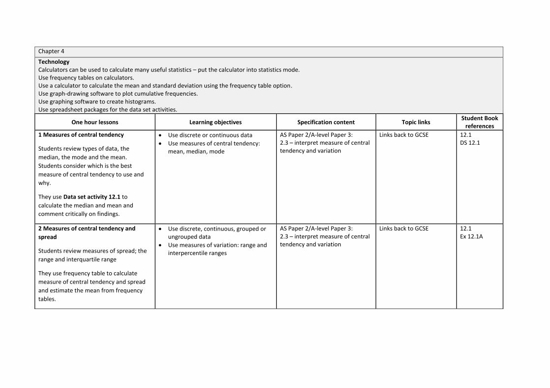
Chapter 4
Technology Calculators can be used to calculate many useful statistics – put the calculator into statistics mode. Use frequency tables on calculators. Use a calculator to calculate the mean and standard deviation using the frequency table option. Use graph-drawing software to plot cumulative frequencies. Use graphing software to create histograms. Use spreadsheet packages for the data set activities.
One hour lessons Learning objectives Specification content Topic links Student Book
references
1 Measures of central tendency
Students review types of data, the
median, the mode and the mean.
Students consider which is the best
measure of central tendency to use and
why.
They use Data set activity 12.1 to
calculate the median and mean and
comment critically on findings.
• Use discrete or continuous data
• Use measures of central tendency: mean, median, mode
AS Paper 2/A-level Paper 3: 2.3 – interpret measure of central tendency and variation
Links back to GCSE 12.1 DS 12.1
2 Measures of central tendency and
spread
Students review measures of spread; the
range and interquartile range
They use frequency table to calculate
measure of central tendency and spread
and estimate the mean from frequency
tables.
• Use discrete, continuous, grouped or ungrouped data
• Use measures of variation: range and interpercentile ranges
AS Paper 2/A-level Paper 3: 2.3 – interpret measure of central tendency and variation
Links back to GCSE 12.1 Ex 12.1A

3 Variance and standard deviation
Students are introduced to variance and
standard deviation and the fact that these
measures use all the data items. Students
go onto calculating variance and standard
deviation using frequency tables.
• Use measure of variation: variance and standard deviation
• Use the statistic
𝑠𝑥𝑥 = ∑(𝑥 − �̅�)2 = ∑ 𝑥2 (∑ 𝑥)2
𝑛
• Use standard deviation 𝜎 = √𝑆𝑥𝑥
𝑛
AS Paper 2/A-level Paper 3: 2.3 – interpret measures of variation, extending to standard deviation 2.3 – be able to calculate standard deviation, including from summary statistics 2.4 – select or critique data presentation techniques in the context of a statistical problem
This is covered further in Book 2, Chapter 13 Statistical distributions
12.2 Ex 12.2A
4 Data cleaning
Recap calculating variance and standard
deviation from frequency tables and then
introduce data cleaning as involving the
identification and removal of any invalid
data points from the data set. Students
use Data set activity 12.2 to clean the
data and give reasons for their omissions.
• Use measure of variation: variance and standard deviation
• Use the statistic
𝑠𝑥𝑥 = ∑(𝑥 − �̅�)2 = ∑ 𝑥2 (∑ 𝑥)2
𝑛
• Use standard deviation 𝜎 = √𝑆𝑥𝑥
𝑛
AS Paper 2/A-level Paper 3: 2.4 – select or critique data presentation techniques in the context of a statistical problem
12.2 DS 12.2
5 Standard deviation and outliers
Student look at data sets that contain
extreme values, if a value is more than
three standard deviations away from the
mean it should be treated as an outlier.
Students use Data set activity 12.3 to
apply what they have learnt so far,
calculating the mean and standard
deviation, and cleaning a section of the
large data set.
• Use measure of variation: variance and standard deviation
• Use the statistic
𝑠𝑥𝑥 = ∑(𝑥 − �̅�)2 = ∑ 𝑥2 (∑ 𝑥)2
𝑛
• Use standard deviation 𝜎 = √𝑆𝑥𝑥
𝑛
AS Paper 2/A-level Paper 3: 2.3 – interpret measures of variation, extending to standard deviation 2.3 – be able to calculate standard deviation, including from summary statistics 2.4 – select or critique data presentation techniques in the context of a statistical problem
Normal distributions are covered in more depth in Book 2, Chapter 13 Statistical distributions
12.2 DS 12.3

6 Linear coding
Students then use linear coding to make
certain calculations easier. They apply a
linear code to a section of large data in
Data set activity 12.4.
Learning from this and the previous three
lessons is consolidated in exercise 12.2B
• Understand and use linear coding AS Paper 2/A-level Paper 3: 2.3 – interpret measures of variation, extending to standard deviation 2.3 – be able to calculate standard deviation, including from summary statistics 2.4 – select or critique data presentation techniques in the context of a statistical problem
12.2 DS 12.4 Ex 12.2B
7 Displaying and interpreting data – box
and whisker plots and cumulative
frequency diagrams
Box and whiskers plots are used to
compare sets of data. The way of showing
outliers on a box and whisker plot and
identifying outliers using quartiles is
explained. Cumulative frequency diagrams
are used to plot grouped data. (0, 0)
should be plotted and the cumulative
frequencies should be plotted at the
upper bound of the interval. Percentiles
are estimated from grouped data.
Interpolation is used to find values
between two points.
• Interpret and draw frequency polygons, box and whisker plots (including outliers) and cumulative frequency diagrams
• Use linear interpolation to calculate percentiles from grouped data
AS Paper 2/A-level Paper 3: 2.1 – Interpret diagrams for single-variable data, including understanding that area in a histogram represent frequency 2.1 – connect probability to distributions
12.3 Ex 12.3A
8 Displaying and interpreting data –
histograms
Students plot histograms and look at the
distribution of the data. They apply what
they have learnt to Data set activity 12.5,
creating a histogram and performing
linear interpolation.
• Interpret and draw histograms
2.1 – Interpret diagrams for single-variable data, including understanding that area in a histogram represent frequency
12.3 DS 12.5 Ex 12.3B
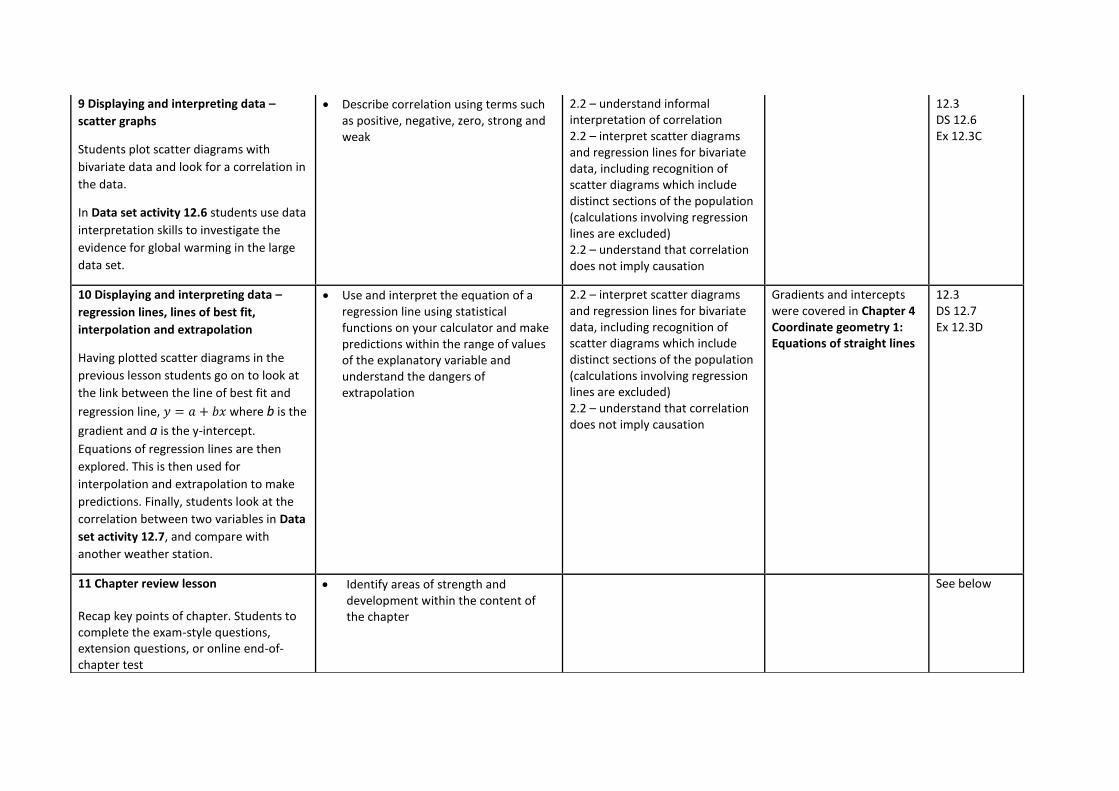
9 Displaying and interpreting data –
scatter graphs
Students plot scatter diagrams with
bivariate data and look for a correlation in
the data.
In Data set activity 12.6 students use data
interpretation skills to investigate the
evidence for global warming in the large
data set.
• Describe correlation using terms such as positive, negative, zero, strong and weak
2.2 – understand informal interpretation of correlation 2.2 – interpret scatter diagrams and regression lines for bivariate data, including recognition of scatter diagrams which include distinct sections of the population (calculations involving regression lines are excluded) 2.2 – understand that correlation does not imply causation
12.3 DS 12.6 Ex 12.3C
10 Displaying and interpreting data –
regression lines, lines of best fit,
interpolation and extrapolation
Having plotted scatter diagrams in the
previous lesson students go on to look at
the link between the line of best fit and
regression line, 𝑦 = 𝑎 + 𝑏𝑥 where b is the
gradient and a is the y-intercept.
Equations of regression lines are then
explored. This is then used for
interpolation and extrapolation to make
predictions. Finally, students look at the
correlation between two variables in Data
set activity 12.7, and compare with
another weather station.
• Use and interpret the equation of a regression line using statistical functions on your calculator and make predictions within the range of values of the explanatory variable and understand the dangers of extrapolation
2.2 – interpret scatter diagrams and regression lines for bivariate data, including recognition of scatter diagrams which include distinct sections of the population (calculations involving regression lines are excluded) 2.2 – understand that correlation does not imply causation
Gradients and intercepts were covered in Chapter 4 Coordinate geometry 1: Equations of straight lines
12.3 DS 12.7 Ex 12.3D
11 Chapter review lesson Recap key points of chapter. Students to complete the exam-style questions, extension questions, or online end-of-chapter test
• Identify areas of strength and development within the content of the chapter
See below

Assessment Exam-style questions 12 in Student Book Exam-style extension questions 12 in Student Book End-of-chapter test 12 on Collins Connect
CHAPTER 13 – Probability and statistical distributions (5 Hours)
Prior knowledge needed Chapter 1 Chapter 12
Technology Use a calculator to perform exact binomial distribution calculations. Use a calculator to perform cumulative binomial distribution calculations.
One hour lessons Learning objectives Specification content Topic links Student Book
references
1 Calculating and representing
probability
Basic probability is recapped and sample
space diagrams are used to determine the
probability of equally likely events
happening. Students go on to calculate
probabilities of mutually exclusive and
independent events using Venn diagrams
and tree diagrams.
• Use both Venn diagrams and tree diagrams to calculate probabilities
AS Paper 2/A-level Paper 3: 3.1 – understand and use mutually exclusive and independent events when calculating probability
Links back to GCSE This will help you in Book 2, Chapter 12 Probability
13.1 Ex 13.1A
2 Discrete and continuous distributions –
part 1
The term discrete and continuous data is
recapped. A discrete random variable is
• Identify a discrete uniform distribution AS Paper 2/A-level Paper 3: 3.1 – link to discrete and continuous distributions
You will use knowledge from Chapter 12 Data presentation and interpretation
13.2 Ex 13.2A

then defined. Probability distribution
tables are used to show all the possible
values a discrete random variable can take
along with the probability of each value
occurring. When all events are equally
likely they form a uniform distribution.
Students go on to probability distributions
of a random variable.
3 Discrete and continuous distributions –
part 2
Continuous random variables are
considered and when graphed a
continuous line is used. The graph is called
a probability density function (PDF), the
area under a pdf shows the probability
and sums to 1. Students then go on to find
cumulative probabilities.
• Identify a discrete uniform distribution AS Paper 2/A-level Paper 3: 3.1 – link to discrete and continuous distributions
You will use knowledge from Chapter 12 Data presentation and interpretation
13.2 Ex 13.2B
4 The binomial distribution
Binomial distribution is about ‘success’
and ‘failure’ as there are only two possible
outcomes to each trail. Students identify
situations which can be modelled using
the binomial distribution. They then
calculate probabilities using the binomial
distribution. Several examples are worked
through.
• Use a calculator to find individual or cumulative binomial probabilities
• Calculate binomial probabilities using the notation 𝑋~B(𝑛, 𝑝)
AS Paper 2/A-level Paper 3: 4.1 – understand and use simple, discrete probability distributions (calculation of mean and variance of discrete random variables excluded), including the binomial distribution, as a model; calculate probabilities using the binomial distribution
You will need the skills and techniques learnt in Chapter 1 Algebra and functions 1: Manipulating algebraic expressions Knowing how to calculate binomial probabilities will help you in Chapter 14 Statistical sampling and hypothesis testing
13.3 Ex 13.3A
5 Chapter review lesson Recap key points of chapter. Students to complete the exam-style questions,
• Identify areas of strength and development within the content of the chapter
See below

extension questions, or online end-of-chapter test
Assessment Exam-style questions 13 in Student Book Exam-style extension questions 13 in Student Book End-of-chapter test 13 on Collins Connect
CHAPTER 14 – Statistical sampling and hypothesis testing (6 Hours)
Prior knowledge needed Chapter 12 Chapter 13
Technology Use a calculator to calculate binomial cumulative probabilities. Use spreadsheet packages for the data set activities.
One hour lessons Learning objectives Specification content Topic links Student Book
references
1 Populations and samples
Discuss the different terms and
terminology within populations including;
finite and infinite population, census,
sample survey, sampling unit, sampling
frame and target population. Move onto
looking at the different types of sampling;
random sampling, stratified sampling,
opportunity sampling, quota sampling and
systematic sampling. In Data set activity
14.1, students compare a random sample
• Use sampling techniques, including simple random, stratified sampling, systemic sampling, quota sampling and opportunity (or convenience) sampling
• Select or critique sampling techniques in the context of solving a statistical problem, including understanding that different sample can lead to different conclusions about population
AS Paper 2/A-level Paper 3: 1.1 – mathematical proof 2.4 – recognise and interpret possible outliers in data sets and statistical diagrams 2.4 – select or critique data presentation techniques in the context of a statistical problem 2.4 – be able to clean data, including dealing with missing data, errors and outliers
You will need to know how to clean data for Chapter 12 Data presentation and interpretation
14.1 DS 14.1 Ex 14.1A

with a systematic sample from the large
data set and draw conclusions.
2 Hypothesis testing – part 1
The two different types of hypothesis are
explained, the null and alternative
hypotheses. 1-tail and 2-tail hypothesis
are explained in relation to a six-sided die.
Having carried out an experiment the null
hypothesis can only be accepted or
rejected based on the evidence, it cannot
categorically be concluded from the
findings.
Students apply what they have learnt in
this lesson in Data set activity 14.2.
• Apply the language of statistical hypothesis testing, developed through a binomial model: null hypothesis, alternative hypothesis, significance level, test statistic, 1-tail test, 2-tail test, critical value, critical region, acceptance region, p-value
• Have an informal appreciation that the expected value of a binomial distribution as given by np may be required for a 2-tail test
• Conduct a statistical hypothesis test for the proportion in the binomial distribution and interpret that results in context
AS Paper 2/A-level Paper 3: 5.1 – understand and apply statistical hypothesis testing, develop through a binomial model: null hypothesis, alternative hypotheses, significance level, test statistic, 1-tail test, 2-tail test, critical value, critical region, acceptance region, p-value 5.2 – conduct a statistical hypothesis test for the proportion in the binomial distribution and interpret the results in context
You will need to know Chapter 13 Probability and statistical distributions
14.2 DS 14.2
3 Hypothesis testing – part 2
Recap previous lesson and students go on
to complete exercise 14.2A
• Apply the language of statistical hypothesis testing, developed through a binomial model: null hypothesis, alternative hypothesis, significance level, test statistic, 1-tail test, 2-tail test, critical value, critical region, acceptance region, p-value
• Have an informal appreciation that the expected value of a binomial distribution as given by 𝑛𝑝 may be required for a 2-tail test
• Conduct a statistical hypothesis test for the proportion in the binomial distribution and interpret that results in context
AS Paper 2/A-level Paper 3: 5.1 – understand and apply statistical hypothesis testing, develop through a binomial model: null hypothesis, alternative hypotheses, significance level, test statistic, 1-tail test, 2-tail test, critical value, critical region, acceptance region, p-value 5.2 – conduct a statistical hypothesis test for the proportion in the binomial distribution and interpret the results in context
14.2 Ex 14.2A

4 Significance levels – part 1
Students look at significance levels being
the probability of mistakenly rejecting the
null hypothesis. The terms test statistic
and critical region are explained and
students move onto finding the critical
region and critical value. They work
through the examples up to the end of
example 5.
• Appreciate that the significance level is the probability of incorrectly rejecting the null hypothesis
5.2 – understand that a sample is being used to make an inference about the population and appreciate that they significance level is the probability of incorrectly rejecting the null hypothesis
14.2
5 Significance levels – part 2
Recap previous lesson, with a focus on
how to calculate values using calculators
instead of statistical tables. After working
through the rest of the chapter from
example 6 onwards, students go on to
complete exercise 14.2B.
• Appreciate that the significance level is the probability of incorrectly rejecting the null hypothesis
5.2 – understand that a sample is being used to make an inference about the population and appreciate that they significance level is the probability of incorrectly rejecting the null hypothesis
14.2 Ex 14.2B
6 Chapter review lesson Recap key points of chapter. Students to complete the exam-style questions, extension questions, or online end-of-chapter test
• Identify areas of strength and development within the content of the chapter
See below
Assessment Exam-style questions 14 in Student Book Exam-style extension questions 14 in Student Book End-of-chapter test 14 on Collins Connect
CHAPTER 15 – Kinematics (10 Hours)
Prior knowledge needed
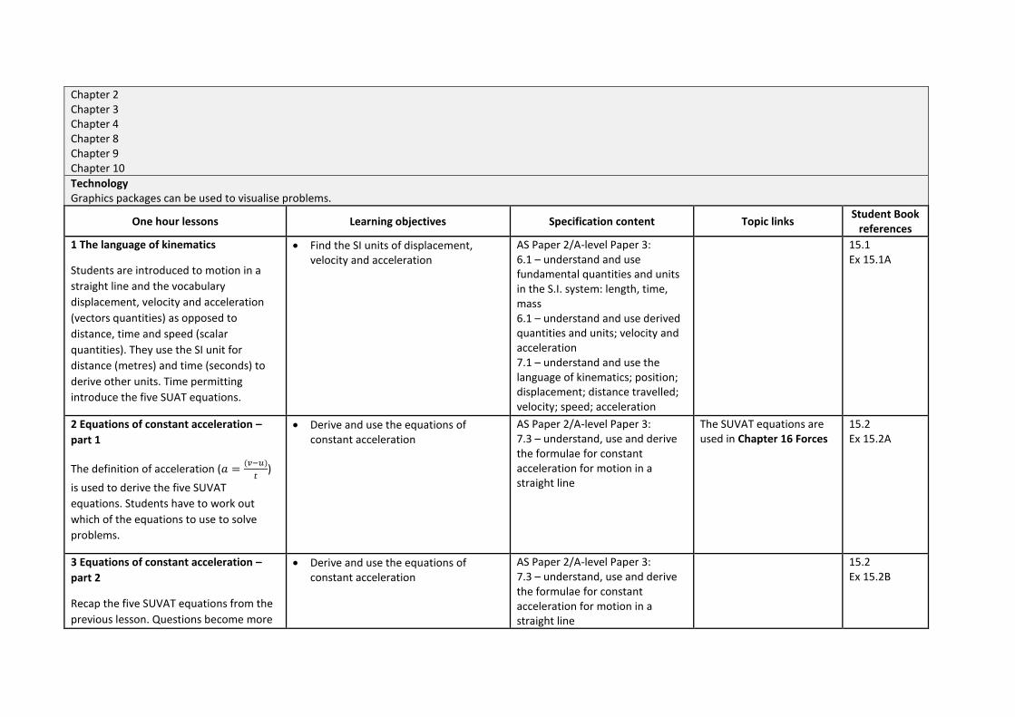
Chapter 2 Chapter 3 Chapter 4 Chapter 8 Chapter 9 Chapter 10
Technology Graphics packages can be used to visualise problems.
One hour lessons Learning objectives Specification content Topic links Student Book
references
1 The language of kinematics
Students are introduced to motion in a
straight line and the vocabulary
displacement, velocity and acceleration
(vectors quantities) as opposed to
distance, time and speed (scalar
quantities). They use the SI unit for
distance (metres) and time (seconds) to
derive other units. Time permitting
introduce the five SUAT equations.
• Find the SI units of displacement, velocity and acceleration
AS Paper 2/A-level Paper 3: 6.1 – understand and use fundamental quantities and units in the S.I. system: length, time, mass 6.1 – understand and use derived quantities and units; velocity and acceleration 7.1 – understand and use the language of kinematics; position; displacement; distance travelled; velocity; speed; acceleration
15.1 Ex 15.1A
2 Equations of constant acceleration –
part 1
The definition of acceleration (𝑎 =(𝑣−𝑢)
𝑡)
is used to derive the five SUVAT
equations. Students have to work out
which of the equations to use to solve
problems.
• Derive and use the equations of constant acceleration
AS Paper 2/A-level Paper 3: 7.3 – understand, use and derive the formulae for constant acceleration for motion in a straight line
The SUVAT equations are used in Chapter 16 Forces
15.2 Ex 15.2A
3 Equations of constant acceleration –
part 2
Recap the five SUVAT equations from the
previous lesson. Questions become more
• Derive and use the equations of constant acceleration
AS Paper 2/A-level Paper 3: 7.3 – understand, use and derive the formulae for constant acceleration for motion in a straight line
15.2 Ex 15.2B

complicated in ex 15.2B and students are
encouraged to draw a diagram to assist
them in understanding the situation
4 Vertical motion – part 1
Students continue to solve problems using the equations of constant acceleration but this time the acceleration is equal to gravity. They need to decide if gravity is influencing the situation in a positive or negative way.
• Derive and use the equations of constant acceleration, including for situation with gravity
AS Paper 2/A-level Paper 3: 7.3 – understand, use and derive the formulae for constant acceleration for motion in a straight line
15.3 Ex 15.3A
5 Vertical motion – part 2 Recap the previous lesson and move on to look at when two objects are launched in different ways, students are advised to look for what the journeys have in common.
• Derive and use the equations of constant acceleration, including for situation with gravity
AS Paper 2/A-level Paper 3: 7.3 – understand, use and derive the formulae for constant acceleration for motion in a straight line
15.3 Ex 15.3B
6 Displacement-time and velocity-time graphs – part 1 Where acceleration is constant, students construct graphs using straight lines and the concepts that the gradient of a displacement-time graphs is velocity and the gradient of a velocity-time graph is acceleration. The area under a velocity-time graph is used to calculate displacement. Students focus on displacement-time graphs.
• Draw and interpret displacement-time graphs and velocity-time graphs
AS Paper 2/A-level Paper 3: 7.2 – understand, use and interpret graphs in kinematics for motion in a straight line; displacement against time and interpretation of gradient; velocity against time and interpretation of gradient and area under the graph
15.4 Ex 15.4A
7 Displacement-time graphs and velocity-time graphs – part 2
• Draw and interpret displacement-time graphs and velocity-time graphs
AS Paper 2/A-level Paper 3: 7.2 – understand, use and interpret graphs in kinematics for motion in a straight line;
15.4 Ex 15.4B

Recap the facts from last lesson and students go on to answer questions focusing on velocity-time graphs.
displacement against time and interpretation of gradient; velocity against time and interpretation of gradient and area under the graph
8 Variable acceleration – part 1 Start the lesson with a quiz on differentiation and integrations. Students use differentiation and integration to solve problems where acceleration is not constant. This lesson focuses on the use of differentiation.
• Use calculus to find displacement, velocity and acceleration when they are functions of time
AS Paper 2/A-level Paper 3: 7.4 – use calculus in kinematics for motion in a straight line: …
Links back to Chapter 8 Differentiation and Chapter 9 Integration
15.5 Ex 15.5A
9 Variable acceleration – part 2 Students use differentiation and integration to solve problems where acceleration is not constant. This lesson focuses on the use of integration.
• Use calculus to find displacement, velocity and acceleration when they are functions of time
AS Paper 2/A-level Paper 3: 7.4 – use calculus in kinematics for motion in a straight line: …
15.5 Ex 15.5B
10 Chapter review lesson Recap key points of chapter. Students to complete the exam-style questions, extension questions, or online end-of-chapter test
• Identify areas of strength and development within the content of the chapter
See below
Assessment Exam-style questions 15 in Student Book Exam-style extension questions 15 in Student Book End-of-chapter test 15 on Collins Connect
CHAPTER 16 – Forces (8 Hours)
Prior knowledge needed Chapter 10 Chapter 15

Technology Graphics packages can be used to visualise problems.
One hour lessons Learning objectives Specification content Topic links Student Book
references
1 Forces
Students are told the SI unit of force is the
newton and mass is the kilogram. They
use vectors, Pythagoras’ theorem and
trigonometry to find resultant forces.
They also use the face that if the resultant
force is equal to zero then an object is in
equilibrium.
• Find a resultant force by adding vectors
• Find the resultant force in a given direction
AS Paper 1: 9.5 – use vectors to solve problems in pure mathematics and in context, including forces A-level Papers 1 & 2: 10.5 – use vectors to solve problems in pure mathematics and in context, including forces AS Paper 2/A-level Paper 3: 6.1 – understand and use derived quantities and units; force and weight 8.1 – understand the concept of a force
Builds on Chapter 10 Vectors
16.1 EX 16.1A
2 Newton’s laws of motion part one
Students are told Newton’s laws of
motion. They apply these to problems.
Students are then introduced to the five
different types of force. These are
represented diagrammatically so that they
are clearly distinguishable. Students then
go on to use simplified models to
represent real-life situation and solve
problems
• Apply Newton’s laws and the equations of constant acceleration to problems involving forces
• Distinguish between the forces of reaction, tension, thrust, resistance and weight
• Represent problems involving forces in a diagram
AS Paper 2/A-level Paper 3: 8.1 – understand the concept of a force; understand and use Newton’s first law 8.2 – understand and use Newton’s second law for motion in a straight line (restricted to forces in two perpendicular directions or simple cases of forces given as 2-D vectors) 8.3 – understand and use weight and motion in a straight line under gravity
16.2 Ex 16.2A
3 Newton’s laws of motion part two • Apply Newton’s laws and the equations of constant acceleration to problems involving forces
AS Paper 2/A-level Paper 3: 16.2 Ex 16.2B

Students are told Newton’s laws of
motion. They apply these to problems.
Students are then introduced to the five
different types of force. These are
represented diagrammatically so that they
are clearly distinguishable. Students then
go on to use simplified models to
represent real-life situation and solve
problems
• Distinguish between the forces of reaction, tension, thrust, resistance and weight
• Represent problems involving forces in a diagram
8.1 – understand the concept of a force; understand and use Newton’s first law 8.2 – understand and use Newton’s second law for motion in a straight line (restricted to forces in two perpendicular directions or simple cases of forces given as 2-D vectors) 8.3 – understand and use weight and motion in a straight line under gravity
4 Vertical motion
Students move from particles travelling
horizontally to particles travelling in
vertically. When particles travel vertically
they have to consider the effects of
gravity and weight.
• Distinguish between the forces of reaction, tension, thrust, resistance and weight
• Model situations such as lifts, connected particles and pulleys
AS Paper 2/A-level Paper 3: 8.3 – understand and use weight and motion in a straight line under gravity; gravitational acceleration , g, and its value in S>I> units to varying degrees of accuracy 8.4 – understand and use Newton’s third law
16.3 Ex 16.3A
5 Connected particles – part 1 More complex problems are solved using Newton’s laws and simultaneous equations due to the consideration of resistive forces. Modelling assumptions are made and shown with diagrams when answering questions. The connected particles considered are particles suspended on ropes, vehicles towing caravans and lifts.
• Model situations such as lifts, connected particles and pulleys
• Represent problems involving forces in a diagram
AS Paper 2/A-level Paper 3: 8.4 - understand and use Newton’s third law; equilibrium of forces on a particle and motion in a straight line; application to problems involving smooth pulleys and connected particles
16.4 Ex 16.4A
6 Connected particles – part 2 Recap on the chapter so far. Students complete exercise 16.4B.
• Model situations such as lifts, connected particles and pulleys
• Represent problems involving forces in a diagram
AS Paper 2/A-level Paper 3: 8.4 - understand and use Newton’s third law; equilibrium of forces on a particle and motion in a straight line; application to
16.4 Ex 16.4B

problems involving smooth pulleys and connected particles
7 Pulleys Connected particles are now considered in the form of pulleys. The main difference being that when an object is connected via a pulley it will be travelling in a different direction. Students should again draw diagrams representing the situation in the question. They solve problems using Newton’s laws of motion, the SUVAT equations and simultaneous equations.
• Model situations such as lifts, connected particles and pulleys
• Represent problems involving forces in a diagram
AS Paper 2/A-level Paper 3: 8.4 - understand and use Newton’s third law; equilibrium of forces on a particle and motion in a straight line; application to problems involving smooth pulleys and connected particles
16.5 Ex 16.5A
8 Chapter review lesson Recap key points of chapter. Students to complete the exam-style questions, extension questions, or online end-of-chapter test
• Identify areas of strength and development within the content of the chapter
See below
Assessment Exam-style questions 16 in Student Book Exam-style extension questions 16 in Student Book End-of-chapter test 16 on Collins Connect

AQA Mechanics 1 – Learning Programme
Autumn Term 1 2017/2018
Week Chapter Learning Objectives Independent Work 1 & 2
(4/9)
(11/9)
2: Kinematics in one
dimension
▪ Define displacement, velocity and acceleration ▪ Understand and interpret displacement-time graphs
and velocity-time graphs ▪ Solve problems involving motion under constant
acceleration using standard formulae ▪ Solve problems involving vertical motion under
gravity
EXERCISE 2B EXERCISE 2C Chapter 2 Test yourself
3
(18/9)
3: Kinematics in two
dimensions
▪ Plot and interpret paths given a position vector ▪ Find magnitudes and directions of vectors ▪ Apply and use the constant acceleration equations in
dimensions ▪ Use velocity triangles to solve simple problems
EXERCISE 3C EXERCISE 3D Chapter 3 Test yourself
4
(25/9)
Term 1a Course suitability assessment
5 - 7
(2/10) (9/10)
(16/10)
4: Forces
▪ Identify the forces acting on a body ▪ Draw force diagrams and resolve forces into
components ▪ Find resultant forces and understand that the
resultant forces is zero when the forces are in equilibrium
▪ Write forces as vectors ▪ Use the friction inequality
EXERCISE 4E EXERCISE 4F EXERCISE 4G Chapter 4 Test yourself

Autumn Term 2 2017/2018
Week Chapter Learning Objectives Independent Work 1&2
(30/10) (6/11)
5: Newton’s laws of
motion
▪ Apply Newton’s three laws of motion ▪ Solve problems where the forces are in equilibrium ▪ Solve problems where a particle is accelerating
EXERCISE 5B Chapter 5 Test yourself
3
(13/11)
6: Connected
particles
▪ Solve problems of motion involving connected particles
EXERCISE 6A Chapter 6 Test yourself
4&5
(20/11) (27/11)
7: Projectiles
▪ Find the time of flight of a projectile ▪ Find the range of a projectile ▪ Find the maximum height of a projectile
EXERCISE 7A EXERCISE 7B Chapter 7 Test yourself
6
(4/12)
Term 1b PPE
(Mechanics 1 Full Exam Paper , 1hr 30 min)
7
(11/12)
8: Momentum
▪ Define the momentum of an object ▪ Understand what happens to momentum of a particle
during collision ▪ Use the principle of conservation of momentum to
calculate momentum after collision, in both one and two dimensions
EXERCISE 8A EXERCISE 8B Chapter 8 Test yourself

AQA Core 3 – Learning Programme
Summer term 2 2016/2017
Chapter Learning Objectives Independent Work 1:
Functions ▪ Understand Function notation ▪ Describe the domain and range for a given function ▪ Find composite functions in the form fg(x) ▪ Find inverse functions
Chapter 1 MIXED EXERCISE Chapter 1 Test yourself
2: Transformations
of graphs and the modulus function
▪ Sketch graphs of the modulus function in the form y=|f(x)| and y=f(|x|)
▪ Solve an equation involving a modulus ▪ Apply a combination of transformations to a graph ▪ Sketch transformations and labelling the co-ordinates of given
point
Chapter 2 MIXED EXERCISE Chapter 2 Test yourself
3: Inverse
trigonometric functions and
secant, cosecant and cotangent
▪ Evaluate secant, cosecant and cotangent functions of angles ▪ Use secant, cosecant and cotangent functions to solve equations ▪ Combine the secant, cosecant and cotangent functions with the
Pythagorean identities ▪ Work with the inverse trig functions; arcsin, arcos, and arctan. ▪ draw the graphs of the inverse functions
EXERCISE 3D Chapter 3 Test yourself
4: The number and
calculus
▪ Recognise the number e ▪ Differentiate and integrate ekx ▪ Use exponential functions and logarithmic functions in calculus
Chapter 4 MIXED EXERCISE

Autumn Term 1 2017/2018
Week Chapter Learning Objectives Independent Work 1&2
(4/9)
(11/9)
5: Further
differentiation and the chain
rule
▪ Find the derivatives of sinx and cosx ▪ Differentiate composite functions using the chain
rule
▪ Use the relationship dy/dx = 1
𝑑𝑥𝑑𝑦⁄
REVISION EXERCISE 5 Chapter 5 Test yourself
2&3
(11/9) (18/9)
6: Differentiation
using the product rule and the quotient rule
▪ Differentiate using the product rule ▪ Differentiate using the quotient rule ▪ Differentiate tanx, cotx, secx and cosecx
REVISION EXERCISE 6 Chapter 6 Test yourself
4
(25/9)
Term 1a Course suitability assessment
5 & 6
(2/10) (9/10)
8: Integration by inspection and
substitution
▪ Integrate expressions using the reverse idea of the chain rule
▪ Integrate trigonometric expressions
▪ Integrate expressions of the form 𝑓′(𝑥)
𝑓(𝑥)
REVISION EXERCISE 8 Chapter 8 Test yourself
7
(16/10)
9: Integration by
parts and standard integrals
▪ Integrate expressions using integration by parts ▪ Use relevant standard integrals quoted in the
formulae booklet
REVISION EXERCISE 9 Chapter 9 Test yourself

Autumn Term 2 2017/2018
Week Chapter Learning Objectives Independent Work 1
(30/10)
4: The number and
calculus
▪ Recognise the number e ▪ Differentiate and integrate ekx ▪ Use exponential functions and logarithmic functions
in calculus
REVISION EXERCISE 4 Chapter 4 Test yourself
2
(6/11)
7: Numerical solution of
equations and iterative methods
▪ Locate roots of equations by change of sign ▪ Use numerical methods to find solutions of
equations ▪ Understand the principle of iteration ▪ Understand how cobweb and staircase diagrams
demonstrate convergence or divergence for equations of the form x=g(x)
REVISION EXERCISE 7 Chapter 7 Test yourself
3
(13/11)
10: Volume of
revolution and numerical
integration
▪ Evaluate volumes of revolution ▪ Use the mid-ordinate rule to find a numerical
approximation for a definite integral ▪ Use Simpson’s rule to find a numerical
approximation for a definite integral
REVISION EXERCISE 10 Chapter 10 Test yourself
4&5
(20/11) (27/11)
Core 3 Revision and
Exam Practice
▪ Revision by topic ▪ Past paper practice
6
(4/12)
Term 1b PPE
(Core 3 Full Exam Paper , 1hr 30 min)