Embed Size (px)
Citation preview

117
EDDINGTON'`S ,STATISTICAL THEORY
III. T H E U N C E R T A I N T Y O F T H E O R I G I N
by
C. W. Kilmister and B. O. J, Tupper (London)
The density-particle correlation, described in a previous paper o f the series, is used to define
the , uncertainty o f the physical o r ig in , considered by Eddington, and to relate it to the Hubble
constant.
1. I N T R O D U C T I O N
1.1 In this paper the arguments of two previous papers (Bastin and Kilmister
1956), referred to here as I, II, are continued to discuss the relationship found
by Eddington, (1946 w 3) referred to here as FT, between the uncertainty of
the origin and the Hubble constant. A later paper will discuss the relation of
the uncertainty with the nuclear range-constant, and so connect that with the
Hubble constant. This will provide a direct experimental check for the theory.
1.2 In I, Eddington's deduction (FT w 1, 2, 3) was described and criticised;
it was noted that while w 1 and 2 required only slight amendment, w 3 was
quite unsatisfactory. A discussion of the concept of order in relation to Ed-
dington's work was also given in I. This was used to explain the status of
work like the present paper, in which substantial numerical agreement is found
with some of Eddington's results, although by quite a different method. In 11
the density-particle correlation was set up. This was suggested by some in-
correct statements of Eddington, but in II the correlation was set up correctly
between two Riemannian spaces. When this correlation was restricted by various 9 - Rend. Circ. Matem. Palermo - Serie 11 - Tomo VI - Anno 1957.
| 1 8 C . W . KILMISTER a n d s . o. J. TUPPER
conditions it was shown in II that it does provide a connection between small-
and large-scale phenomena. However this connection is not altogether satisfac-
tory, since the large-scale constant involved is not measured. In the present
paper it is argued that the conditions imposed on the correlation in II were
too restrictive. The correlation is then considered in a more general case.
1.3 The basic physical idea of the present paper is that the density-particle
correlation is an important way of relating small-and large-scale constants. The
more general method of applying the correlation, which is employed here, does
provide a satisfactory method of relating the Hubble constant to the uncertainty
of the origin, without any of the obscure arguments of FT.
2. THE PHYSICAL ORIOIN
2. 1 It was found in I that w167 1, 2 of FT were mostly satisfactory, although
small amendments were required. For the sake of completeness, however, it is
desirable to reproduce the amended arguments here. This section will therefore
follow FT fairly closely. The basis of relativity theory is the recognition of the necessity for a
coordinate system in describing physical phenomena. From this basis the theory
then goes on to find how to ensure that we are not merely investigating pro-
perties of the coordinate system employed. It does this by considering a set
of coordinate systems, and defining the group, G(Z), of all transformations
S -~S ' , where S, S' belong to ~:. A first necessary requirement that we are
investigating physically significant properties is then that they should be true
in all the coordinate systems of Z. Since these properties are to be expressed
by numbers and relations between numbers, these numbers must transform
under a representation of the group G(Y). This condition is a general formula-
tion of the �9 principle of relativity~; the usual tensor theory then follows.
However, in this paper, we are concerned only with the initial step in this
derivation, that is, with the recognition of the necessity for a coordinate system.
2.2 The principle of relativity is a necessary condition of physical signifi-
cance of properties, but it is not a sufficient one. This fact has been shown by
quantum theory. A possible basis for quantum theory, the uncertainty principle,
can be expressed in the following form, which has the advantage for us that
it is intimately connected with 2.1:

EDDINGTON'S STATISTICAL THEORY 1 19
The numbers describing a physical system, in the sense of 2.1, can be
divided into classes of conjugate pairs. It is false to suppose that both members
of a class can be known exactly. If one member is known to a certain uncer-
tainty, the minimum uncertainty of the other is specified by the uncertainty
relation.
These uncertainties must, of course, be defined accurately in terms of pro-
bability distributions. When this has been done, the usual formulation of quantum
theory can be built up. As in 2.1, w e are concerned only with the first step
in this derivation. We shale consider, in particular, the position of particles. The
conjugate variable is then related to the momentum; however, the form of the
restriction which is sufficient fc.r our purposes is simply that the position can
only be known with some uncertainty, that is, that a probability distribution
is given for the position.
2.3 Many quantum physicists have insisted that the equations of quantum
theory should be Lorentz invariant, but Eddington (1939) put forward the fol-
lowing argument against this view:
The formal conditions of Lorentz-invariance apply to coordinates tx~, xz, x3, ix~)
which form a four-vector, and to expressions associated with them. If (x~, y~, z~, it1)
and (x2, Y2, z2, it2) are two four-vectors and
= x~ - - x2, ~ = y, - - y~, ~ = z~ - - z2, ~ = t, - - t2, (2.3.1)
then ({, r~, ~, it) is a four-vector. The transformation conditions to be satisfied
by ~, ~, ~, z and associated expressions are identical with those for x, y, z, t
and associated expressions. Hence, formal conditions of Lorentz-invariance apply
to wave functions, etc., formed with relative coordinates ~, ~, ~, z as well as
those formed with x, y, z, t. The space coordinates usually employed are indeed
{, ~, ~ but z is never wittingly employed. Instead a progressive time coordinate
t is taken, so that ~, "q, ~, i t is not a four-vector and wave functions r "~, ~, t)
are not Lorentz-invariant. Nevertheless, conditions of Lorentz-invariance are applied
by many authors. Alternatively, they attempt to base the investigation on wave
functions of non-relative coordinates x, y, z, t. Eddington pointed out that such
wave functions give no information about the eigenstates, and that there is no
means of deriving wave functions of ~, "q, ~ from those of x, y, z.
Dirac, Peierls, and Pryce (1942) defended the text-book treatment of quantum
theory by saying that the equations are approximate and are not Lorentz-invariant,
1 2 0 c . w . KILMISTER a n d B. O. J. TUPPER
but are approximately so. That is, the equations used in one frame L, when
transformed to another frame L', are not exactly equivalent to those used in L,
but only so within the accuracy of the approximation involved. However, in
his reply, Eddington (1942) insists that the error of the text-book treatment, as
elaborated by Dirac, Peierls, and Pryce, is a fundamental fallacy and not a
lack of rigour, and gives an example which, he asserts, does not result in
merely an imperfect approximation to the conditions which Dirac's Lorentz-
invariant equation expresses, but results in conditions which are precisely op-
posite to those which the equation expresses. Again, in FT (p. 117), Eddington
says, ,r Lorentz transformations become ineffective in statistical physics; for we
have seen that the time coordinate is differentiated from the space coordinates
at the outset of the study of the probability distributions. The curious insistence
on introducing Lorentz transformations, which appears so often in the literature
of quantum theory, is an example of the introduction of mystification which
can have no other purpose than to give the mathematician an opportunity of
removing it *.
We will here follow Eddington's view and not insist that the results should
be Lorentz-invariant. When we have found non-invariant results it may some-
times be possible to deduce Lorentz-invariant results by the usual method of
generalisation. This process may be thought of as analogous to that of using
a special coordinate system for a given problem.
2.4 If we are to consider the positions of a number of particles relative
to a given coordinate system, each position must then be specified by a pro-
bability distribution. It is convenient to avoid the consideration of so many
independent distributions by recalling that the uncertainty was introduced me-
rely to conform to the uncertainty relation. We therefore introduce an uncertain
origin specifying a coordinate system K; we are then considering a different
kind of coordinate system from those understood in 2.1 and 2.2, and the trans-
formations S - ~ K does not belong to G(~). We may suppose the coordinates
of a particle relative to K to be known exactly, since the uncertainty has been
provided, once and for all, by the origin, it should be noted here, however,
that although (x~), (yi) may be exactly known coordinates of particles X, Y re-
lative to the coordinate system K (here supposed rectangular cartesian) the di- stance X Y will not be known to be exactly IZ(x i - yi)~]l/2, for if we consider
both X and Y allowance must be made for them to have independent proba-
bility distributions.

EDDINCTON'S STATISTICAL THEORY 121
2.5 It is necessary to be able to specify the transformation and, in order
to do this, we must know the probability distribution of the origin. We are
here faced with a difficulty, since we require to know the frequency function
f(x~), say, of the position x~ of the origin of K relative to S. Now f cannot be
found by observation, since the x~ are not observables. On the other hand, the
coordinates postulated in the dynamical equations of quantum theory are assumed
to be observable, and must therefore be measured relative to K. The equations
are certainly not invariant under arbitrary changes of the function f, so that
they must imply a special choice of probability distribution. The special choice
which must, in fact, have been made by quantum theory is suggested by the
Central Limit Theorem (Kendall 1945 p. 180). A consequence of this is that
the centroid of a large assembly of non-interacting particles has a (3aussian di-
stribution, no matter what distribution (within certain limits) the particles may
have. If there are N particles, each with standard deviation k, then the standard k
deviation of the centroid is - ~ - . Thus, if we postulate the centroid of N par-
ticles as (x~), the function f is determined. There seems to be no other equally
simple choice of definition. This fact and also the numerical agreement of the
results found in a future paper with quantum mechanical experiment suggest
that this is the choice made by quantum theory. There remains only the deter-
mination of the standard deviation, k, of each particle.
2.6 Before proceeding to this, let us consider this requirement imposed by
the Central Limit Theorem that the particles are non-interacting. It will clearly
be illegitimate to allow charged particles to enter, and so we take particles as
hydrogen atoms. (It is unnecessary to explain again here how we may restrict
our attention to a particularly simple theory in which all the particles are taken
as equal. It is explained in I in what sense such a theory is useful in describing
the universe). However, there is still the gravitational force between the particles,
but this may be disregarded if we assume the particles to be in a space-time
manifold of general relativity; the gravitational field will then be represented
in the geometry of the space. (Eddington seems to have been unaware of the
necessity for non-interacting particles in FT). The use of a curved space raises
a difficulty in the definition of the centroid in a non-invariant manner. However,
we require the idea of a centroid to define the origin of a certain coordinate
system, and we accordingly use a coordinate system of the same kind to cal-
culate the centroid.

122 c.w. ]KILM|STER and B. o. J. TUm'ER
3. FIRST SPECIFICATION OF THE DISTRIBUTION
3.1 We are then committed to a statistical theory in a curved space-time,
even though the theory will not be Lorentz-invariant. We have to consider
sections of the space-time by space-like three-surfaces corresponding, in some
particular coordinate system, with surfaces of constant time. If we adopt such
a coordinate system, the metric for any section will have the form
d s 2 ~ gi~dxi d x i,
where i, j take the values 1, 2, 3 and gij is a positive definite quadratic form.
It is well known that in general relativity the coordinates cannot have their
usual significance and one of the problems of the present paper is to use the
physically significant coordinates.
3.2 It is necessary to remark on the exact status of the standard deviation
k as a physical constant. It is the standard deviation of the distribution of a
single particle. This is not, of course, meant to imply that there is one uniquely
determined distribution. Rather we must define, by some precise process, a
distribution which it is natural (in some sense) to consider for a particular
space-time. This is clearly the most difficult part of the theory. Eddington's
argument (FT w 3) in terms of volumes rests on the assumption that the standard
deviation is settled at a more primitive stage in the theory than that at which
length measurement enters. The standard deviation can then be used to define
a unit of length, and so determines also the radius of the universe. Apart from
Eddington's error in calculation (|, w 4.4), it is at least doubtful whether the
standard deviation or length m e a s u r e m e n t is more primitive. In the present
section one suitable definition of a distribution will be put forward and the
resulting standard deviation will be calculated. This definition has the merits
of simplicity and obviousness, and seems to be close to that intended by
Eddington. The rest of the paper will be taken up with the consideration of
another distribution, defined by the mass-particle correlation, (II).
3.3 In the metric of (3.1) there is defined at every point the
ment of proper volume
d v - -
The distribution considered in this section is then defined by
invariant ele-
E D D I N G T O N ' S S T A T I S T I C A L T H E O R Y 123
Definit ion 1. The particles are distributed randomly per unit proper volume.
We shall first illustrate the calculation of the s tandard deviation for this
distribution in an Einstein universe, in order to compare with Eddington's re-
suit. We shall then carry out the calculation in an expanding universe.
The Einstein universe metric is usually written
d s 2 __ d r 2 - - r 2 + r2(d02 + sin2 0dr (3.3.1)
1 - - - - R '
We then have
d V - - r 2 s i n O d r d O d % (3.3.2)
Thus the chance of finding the particle in the range (r, r + dr) would be d
proportional to dr. No interest attaches, however, to finding the stan-
dard deviation of such a distribution, since r is not a measured coordinate. If
we write r ~ / ? sin X, we have
d s ~ = R 2 [ d x 2 + sin 2 x(dO 2 + sin ' Od~2)],
which shows RX to be the measured radial distance. In terms of X we have
1 A P d r - - A sin s X d X ~- -~- A d(x - - sin X cos X), (3.3.3) d
I./1 _ N where A is a constant. For (3.3.3) to define a probability distribution we have
1-- A . I d - -
g=0
sin X cos X) = 1,
(the limits being fixed as the values of X for which d V vanishes), which gives
A = --.2 The second moment about the mean, , is thus
5f( ~-a = - - d(x ~ sin X cos X) =
:t=O
The standard deviaton of X is ~/~2 = 0.568, so that k = 0 . 5 6 8 R = 1~76T" This

124 c .w. KILMISTER and a. o. J. TUPPER
gives the value of Eddington's uncertainty
R R Eddington's ~ -~ - or Slater's
3 1 ~ "
constant as R 1.761 ~/~"
instead of
3.4 Consider now an expanding universe of the standard form
_ R 2 ds2 ~ /1 + I v ( d x ~ -J- dx~ -~- dx~),
T1
corresponding to the case of a space of positive curvature. (For spaces of ne-
gative or zero curvature this definition is not of any use). First make the sub-
stitution
R X i = Xl,
so that
d s 2 =
The metric becomes
~ r = F .
l i a 2 ( d x ~ + d x ~ + d x ~ ) .
m
If we now put r = 2t? tan (;(/2), so that
ds 2 = R2[d;( 2 + sin 2 ;((dO 2 + sin: Od~2)],
we have the same form as before. The standard deviation is again 0.568/?.
This agreement is actually a physically significant one, and not merely formal. 0.568
We can see this by expressing each standard deviation as 2 ~ X (greatest
measurable length).
4. THE DENSITY-PARTICLE CORRELATION
4.1 In the rest of this paper we shall investigate the problem of using the
density-particle correlation to define an alternative distribution to that used in
w 3. This is done by supposing that the function q~ in the density particle
correlation (II) is in some respects analogous to a ~-function in the quantum-
mechanical sense. Accordingly it is natural to consider the distribution of par-
ticles with density qj2 per unit proper volume. Since it will be shown that a

EDDINCTON'S ST&TISTICAL THEORY 1 2 5
possible solution of the correlation, for a suitable expanding universe, is one
independent of the space-coordinatesi the distribution of w 3 arises as a special
case. The present paragraph is concerned with finding solutions of the density-
particle correlation. In II, we made the following assumption about the density-
particle correlation :
(i) the total number, N, of particles in S is finite and constant;
(if) the rest-mass, m0, of particles in S is constant;
(iii) the total mass in ,S is constant.
These assumptions, together with the condition p = 0, which was imposed in
order that the energy tensor,
T ~ = (p + ~c2)v~v ~ - p g ~ , (4.1.1)
should be factorisable, are sufficient to reduce S, S, to Einstein universes, in-
stead of expanding universes. It therefore appears that assumption (i), and con-
sequently (iii), may be too strict. Hoyle and his fellow workers have produced
a cosmology in which a continuous creation of matter takes place, so that it
would be quite reasonable to drop the first assumption. Accordingly, we shall
now begin by considering the density-particle correlation with no limitations
in the form
C 4 where D = C . . . .
8 ~ KM is the Einstein tensor,
G~13~ = D ~ n l ~ , (4.1.2)
and C is an arbitrary, non-zero, numerical constant, G ~
n " ~ - - - - g ~ ; ~ , and, from II, ~ is a scalar.
4.2 We shall first seek solutions of (4.1.2) with spherical symmetry, in an
expanding universe, in this sense: that G ~a is the Einstein tensor of S, and
the covariant differentiation in (4.1.2) is carried out in S, as in II (w 5.2). S will
be taken to be an expanding universe with the metric
where A = I + - - - -
R2(t ) , - d s 2 = d t 2 -~ tax -]- d y 2 + dz2), (4.2.1)
k P 74 and k is • 1 or 0. The value k = 1 corresponds to a
finite universe, while the value k = 0 has been shown by McCrea (1951)to be
a necessary condition for a steady-state universe. The metric of S is of the form
-- d~ d s 2 = e2~dt 2 A2 (dx 2 + d y 2 + dz2). (4.2.2)

126 c .w. KILMISTER and B. o. j. TUPPER
Since we are now imposing no additional conditions on the density-particle
correlation, cr will be a function of x, y, z and t. However, we shall be inte-
rested in applying the theory only when S is one of the well-known cosmolo-
gical models, and we shall therefore restrict ': by the cosmological principle.
That is to say, ~ will be a function of t only.
We may write (4.1.2) in the form
1 [R~ - - ~ -g~ (R - - 2 k)] 02 = D 02; ~ (4.2.3)
where ), is the cosmical constant. The values of the Christoffel bracket symbols
in S and S can easily be calculated and these lead to the following values for
the components of the Ricci tensor in S and its contraction:
R,, = R~ = R~ - - ~ 2 - ( 2 k + 2 R ~ + ~R) ,
3R ( k k ~ J~\ R . = -R-' R = 6 )~- + R~ + ~-) .
Note here that we have put the velocity of light, c, equal to unity to simpIify
the working. The dimensions will be corrected in our final results.
The equation (4.2.3) gives the following ten equations for 02
1 /~ A5 (k + + 2 R ~ i - - XR2)02 = D02;,,
k x k y k z ~ ( [ ? R~)02,,!, = D [02,,, + -2-~ 02,' 2 A 02,2 - - -2-A 02,3 - - +
1 1~ h-~(k + + 2R]~ - - ),R2)02 = D02;~
k x k y ~ k z -Rhx([~ R~) = D{~2,22 2 h 02'' ~ 2-A02"- 2A 02,3 - - + 02,,},
1 1~ A2 (k + -+- 2 R R - - ~,R2)02 = D02;3 3
k x k y k z ~ - ( k = D{02,a3 2 h 02" 2 h 02'~ -{- 2 A -02a - + R o') 02,,},
( ~, - - ~ - - R2 ] 0 2 ----- D O 2 , , , = D ( 0 2 , , , - - a02,,),

~DDINCTON'$ STATISTI~,AL THEORY 127
ky kx 9;,2 = 9,,~ + - ~ 9 , , + ~ 9 , ~
kz ky 9;53 = qJ,. + ~ 9 , ~ + ~0~,~
kx kz 9;3, = 9,3, + 2-~9,~ + ~ 9 , ,
9;,, = 9 , . - - ~ + - R 9,, = 0,
9 ; . = 9 , . - - ~ + y 9 , ~ = o ,
( R) 9;~, = 9,3, - - ~ + ~- 9,3 = o.
We integrate the last three equations and derive
= 0,
= 0 ,
= 0,
9 , t = R e ~ f ~ ( x , y, z), say ( i : l , 2, 3,).
Hence we have
9 = F(x, y, z)Re ~ + a(t).
Substituting in the fifth equation of (4.2.4) we find
F,,2 + k_yF _[_kx 2 " ~ F , 2 = 0 ,
that is
kx (D~ ky
_ ky 0 Putting (D 2 -[- ~ ) F where D~ c3 x~"
(Aep),, = O.
A �9 = b, (y, z),
(a e),~ = b, (y, z).
so that
It follows that
say, and so
= �9 we have
(4.2.4)
(4.2.5)
(4.2.6)
(4.2.7)

128 c . w . ]KILIh~LSTIER and B. o. ~. 'ruepm~
Similarly, by factorising (4.2.7) in the form
+ +
we find that
= O,
(a~,, = a,(x, z).
In a similar manner, we find:
( A F ) , 3 = Cl (y , Z); ( A F ) , , -~- a a ( X , y ) ;
(aF) ,2 = b2(x, y); (aF) ,3 = c,(x, z).
From these equations it follows that
(a F), , = a (x),
(a F),2 = b (y),
(a F),3 = c (z),
which leads, with the conditions of spherical symmetry, to
Pta + Q F - - A
Pr~ + Q Re ~ + G(t).
Hence we have
Substituting this value for tp in the first four equation then to satisfy:
(k + R~ + 2RJ~-- XR2)[I(Pr~ + Q)Re~ 1 + O i
: D(2P-- -~-Q) ( 1 - ~r~)Re~-- D(PP + Q)(R + R~)2Re ~
- -D(1 + - ~ ) (/~ + R~)RG,
(~,-- Rk2 3]?2~I(PP + Q)Re ~ +(1 + ~ ) G I] R 2 / I I
= D(PP + Q){/~ + R~ + R'~}e ~ -+ D(1 + ~ ) ( G -- G~).
and
(4.2.8)
(4.2.9)
(4.2.10)
of (4.2.4) we have
(4.2.11)
(4.2.12)

EDDINGTON'S STATISTICAL THEORY 129
Equating coefficients of fl and terms independent of r in (4.2.11) and (4.2.12)
we have :
= - - D ~ -
(k + + - - XR )(Q ?e ~ + O)
= D(2p k Q)ReO DQ(R + R~),Re, D(i? + R.)RG ' ( 4 . 2 . 1 3 )
(), 3Rk 3-R~ )(Q Re + G)= DQ(]~ + R(~+ R(~)e~ + D(G--G ~).
From the first two of these equations we then find that either
k + R ~ - - ] - R R - X R 2 : - D { k + ( R + R ~ ) 2 } , that is
(1 -t- D)(k + /~2) + 2RR --t- DR~(21~ + Ra) - - I R ~ = 0, (4.2.14)
k or else P - - ~ -Q = 0, since neither R nor e ~ can vanish. From the second two
we have either
3(k +/~2) + DR(]~ -t-/~ ~ + R ~ ) - ~.R 2 = 0, (4.2.15)
k k or P--~Q = 0. Note that the condition P - - ~ - Q = 0 gives the value of ~ as
qJ=QReOq-G, that is, a time-dependent solution only. We wish to consider only solutions
which depend on the space coordinates as well as the time since we intend
to use the space-dependent part as a frequency function to calculate the un-
certainty of the origin. If we were to-select a space-independent frequency
function we should merely be duplicating the results of w 3.
The equation (4.2.10) will now give us a solution for q~ so long as we can)
determine the function G(t), and can solve the simultaneous equations for R, r
(4.2.14) and (4.2.15). We may notice here that if we had retained the condition
p = 0 this would have led, using (4.2.14), to the result
k + (/~ + R~) ~ = 0, (4.2.16
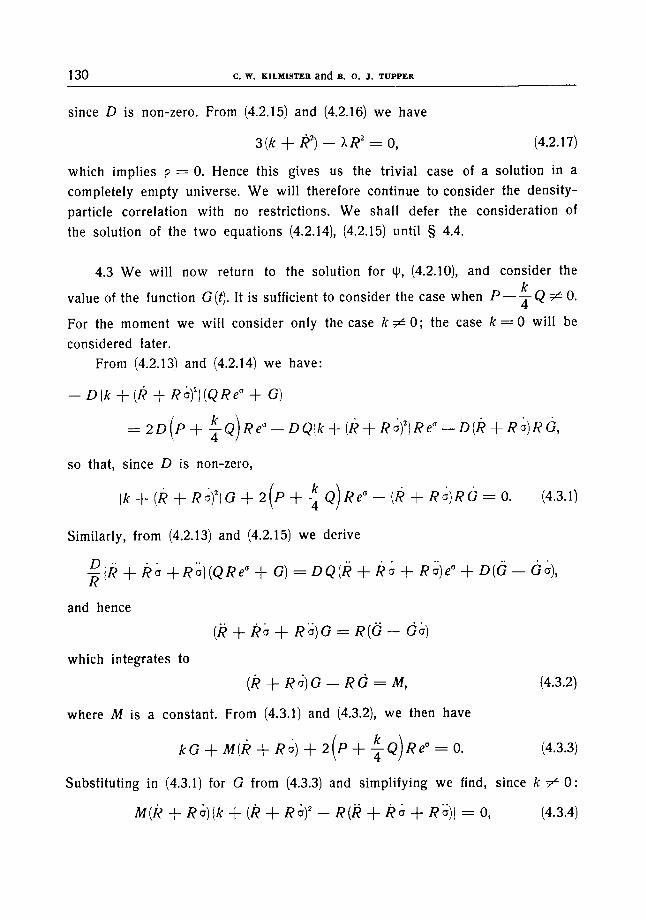
130 c.w. KILMISTER and s. o. ~. TUPPER
since D is non-zero. From (4.2.15) and (4.2.16) we have
3(k + 1)2)_ ).R 2 = 0, (4.2.17)
which implies ~ = 0. Hence this gives us the trivial case of a solution in a
completely empty universe. We will therefore continue to consider the density-
particle correlation with no restrictions. We shall defer the consideration of
the solution of the two equations (4.2.14), (4.2.15) until w 4.4.
4.3 We will now return to the solution for qJ, (4.2.10), and consider the k
value of the function G(t). It is sufficient to consider the case when P - - ~ Q ~ O.
For the moment we will consider only the case k ~ 0; the case k = 0 will be
considered later.
From (4.2.13) and (4.2.14) we have:
-- D{k 4- (1~ @ Ro)2}(ORe ~ -4- G)
k Q)Re ~ D q t k + (R-}- R @ t R e ~ - D(R-}- = 2 D ( P 4- ~ , �9 RolRG,
so that, since D is non-zero,
!k @ (R @ R@}O @ 2 P 4- -~Q Re~ -- (R @ R~)RG =- O. (4.3.1)
Similarly, from (4.2.13) and (4.2.15) we derive
R {R 4- R~ -4-R~}(QRe ~ + G) = DQ(R --}- R[~ 4- Ro)e ~ 4- D(G -- Go),
and hence
which integrates to
(,~ +/)~ + Ri~)O = R(O - 0;)
(/) 4- R o)G -- R d = M, (4.3.2)
where M is a constant. From (4.3.1) and (4.3.2), we then have
+ + + +
Substituting in (4.3.1) for G from (4.3.3) and simplifying we find, since k-~ 0:
M(/) + R6){k + (R + R@ -- R(R, + / ) o + R~)} = O, (4.3.4)

E D D I N G T O N ' S S T A T I S T I C A L T H E O R Y 131
so that we have the three cases
o r
o r
k + / ~ = o
k + (k + R~) ~ - Rik + k~ + R~) = o.
Case (i) M = O. From (4.3.2/, we have:
( k + ~ ) O - - R G = 0 ,
which integrates to
G = A R e ~,
where A is a constant. From (4.3.3) and (4.3.5) it follows that
A = - - 2 ~ - - t - ,
so that, f rom (4.2.10), we have
qj Pr2 + Q R e ~ 2 ( P Q) =- a - k - + Re~'
that is,
k d _ _ _ _ _ _
q ~ = ~ O - - - ~ .
k Since P - - -4- Q ~ 0, we may write this
kd _ _ _ . . . .
4 ~ = H Re ~,
where H is a constant.
Case (ii) I~ + I# a = O.
This condition integrates to
R e ~ = A,
where A is a constant, so that from (4.3.1) we have
(4.3.5)
(4.3.6),
(4.3.7)

132 c . w . KILMISTER a n d B. O. J . r V P p z r t
which gives
From (4.2.15) we have
that is p = - 0 , which leads
0 = O. (4.3.8)
3 (k q- R 2) - - ),/?2 = 0,
to p = 0. This case is therefore
(4.3.9)
trivial, since it
gives a solution only in a completely empty universe.
Case (iit~ k + (R q- R~) 2 - - R0~ + / ? ~ + R~) = 0. (4.3.10)
This condition integrates to
k @ (t~ @ R'~) 2 = A R 2 e 2~ (4.3.11)
where A is a constant. From (4.2.14), (4.2.15) and (4.3.10) we also find that
k + ~,~ - / ? # = o, which integrates to
k + 17 = B / ? 2, (4.3.12)
where B is a constant. From (4.3.11) and (4.3.12), v:e then have:
R~(2 /~ + / ? ~ ) = (Ae 2~ - - B) /? ~,
that- is
3 B q- A D e 2~ = ),.
Hence, either e 2~ must be a constant or 3B = k and A - - 0 . This latter condi-
tion leads to
k + (K' + / ? ~)' = o,
which, from (4.2.14), leads to p = 0 and also ~ = O. As before, this gives a
solution in an empty universe. The other alternative, that e 2~ is constant, implies
e2O 1 ). - - 3 B D A
But from (4.3.11), (4.3.12) A = B when cr = 0, so that comparing (4.2.14), (4.2.15)
with (4.3.10) when ~ = 0, we find that
). = ('3 + D ) B , (4.3.13)
and hence that e 2 ~ = 1. In this case, from (4.3.12),
-
R = cosh VB(t + ~), (4.3.14)

E D D I N G T O N ' S $ T A T I S T [ C & L T H E O R Y 133
where ~ is a constant. From (4.3.3) and (4.3.14) we then have
M G - - t/~-sinh I/B (t q - c ~ ) - - 2 ( P - q - ~ ) [ / / ~ c o s h ~ / B ( t ~ - ~ ) ,
so that (4.2.10) gives
I _ _ _ _
~g-----H
k?
b cosh t~BB(t --[-- ~) - - t/B-(t-[ - ~). (4.3.15) --~k- sinh
The conclusions of 4.2, 4.3 can be summarised as follows: There are two
types of space-dependent solutions of (4.1.2), subject to the conditions stated.
Each type implies that the universe is a definite cosmological model. These
types are
Type I
k?
qJ = H A / cosh ~-/~(t + ~) - - ~ sinh I/B-(t --]-- m),
), where B - 3 ~ D ' and H, M, ~ are arbitrary constants. This corresponds to
a model in which
= cosh I (t +
and holds only when e 2 ~ 1.
Type H kP
1 4
qJ = H ~ Re ~,
where H is an arbitrary constant. The corresponding model is that in which k
satisfies
(i -~ a)(k -[-/~2) + 2 R R q- DR~(2,/? + R~) -- ),/?2 : 0,
3(k q-/?~) -1- D R ( R q- ~ q- R~) - - ),R 2 = O.
4.4 The equations (4.2.14), (4.2.15) (just quoted) are extremely difficult to
solve in the most general case; it is found that multiple singularities occur 10 - Rend. Circ. Matem. P a l e r m o - S e r i e I I - T o m o V I - A n n o 1957

1 3 4 c . w . KILM|STER a n d B. O. J. TIJPPER
when D = 2 or D = - 3. In order to progress any further some simplification
must be made. In this section we shall discuss some particular solutions of
type il by supposing that o is subject to the perfect cosmological principle, so
that it is also independent of t. We can then take e " = 1 without loss of ge-
nerality, so that S, S are the same space. It is then possible to regard (4.2.3)
as a generalisation of gravitation (which is the case corresponding to D-----0).
In this case the equations for /~ become
(1 + D ) ( k + k 2)+2 RR-- XR 2=0,~ 3(k + /~2) + D R ~ - - ) .R 2 := 0.
By subtraction, we have either that D = 2 or else that
(4.4.1)
k + R 2 = R/~. (4.4.2)
1 k + -3-;~ R 2, (4.4.3)
again
If D = 2, the equation integrates to
/ ~ 2 _ A R ~
where A is constant. On the other hand, if (4.4.2) is satisfied we have
the solution of type I.
We have therefore found just one new solution of type II of the form
(4.4.4.)
k r ~ 1 - - -'-'j-- R e ~,
, g = H - A
where R satisfies (4.4.3), and D = 2.
4.5 In this paragraph we make the solutions we have found more explicit,
by assuming that the cosmological models concerned start expanding from an
initial Einstein state. Only the case k = 1 will be considered, since the case
k = - - 1 is not common in cosmology. 1
Consider first type 1. Initially, when l = 0, R = / ~ o - I/~.-, so that
1 cosh~fB ~. B = - - ~ Ro
1 it follows that B : > / - ~ , so that 0 < 3 + D - _ < 1, that is, - - 3 < D - - _ < - - 2 .
t,0
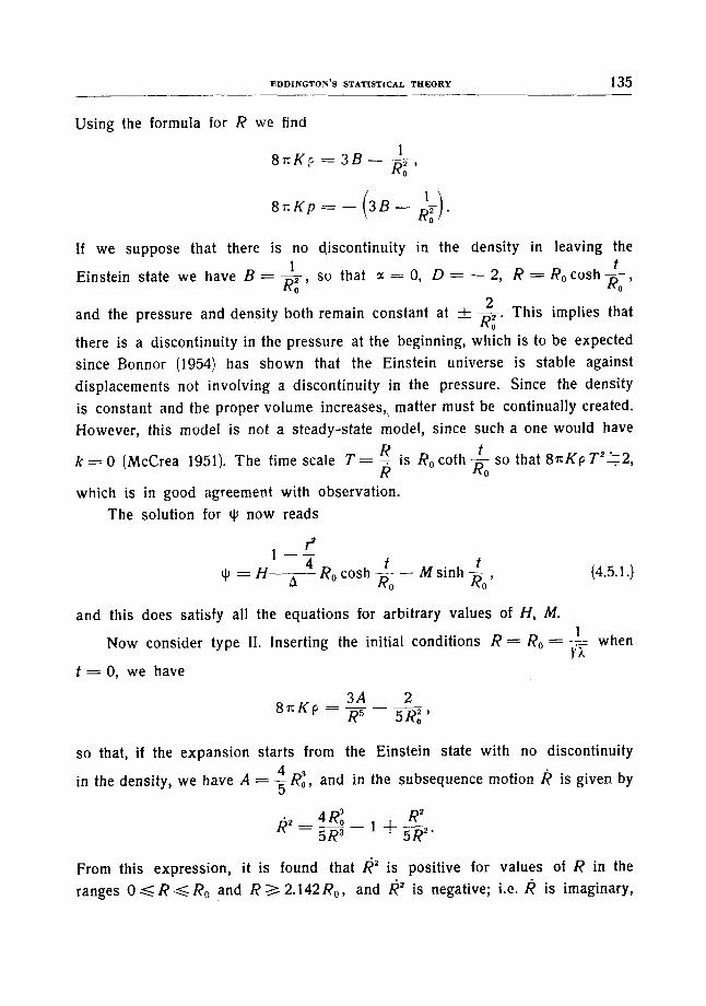
EDDINGTON'S ST&T[S'I['ICAL THEORY 135
Using the formula for /? we find
1 8 ~ K ~ = 3 B - /~-,
8 = K p - = - - 3B---t?~o .
If we suppose that there is no discontinuity in the density in leaving the 1 t
Einstein state we have B : ~ - , so that :~----0, D = - - 2 , R - - - - -Rocosh~- ,
2 and the pressure and density both remain constant at + ~ . This implies that
- - R 0 there is a discontinuity in the pressure at the beginning, which is to be expected
since Bonnor (1954) has shown that the Einstein universe is stable against
displacements not involving a discontinuity in the pressure. Since the density
is constant and the proper volume increases, matter must be continually created.
However, this model is not a steady-state model, since such a one would have
k : 0 (McCrea 1951). The time scale T : ~R is R0 coth Rot so that 87:Kp T2~. 2,
which is in good agreement with observation.
The solution for r now reads
r ~ 1 - - - -
t t q~ = H-- Ro cosh ~5 ~ - - M sinh --Ro ' (4.5.1.)
and this does satisfy all the equations for arbitrary values of H, M. 1
Now consider type II. Inserting the initial conditions R = Ro = - . - - when I'),
t = 0 , we have
3A 2 8 r : K p - R5 5Ro2,
so that, if the expansion starts from the Einstein state with no discontinuity 4
in the density, we have A = -~ R~, and in the subsequence motion /~ is given by
4R o R 2 - 5 R 3
From this expression, it is found that /~ is positive for values of R in the
ranges O~<R~<Ro and R>~2.142Ro, and /~ is negative; i.e. /~ is imaginary,

136 c . w . KILMISTER a n d B. o. j . TUPPER
for /? such that /?o < /? < 2.142/7o. Hence, if this model is initially in the
Einstein state, it will contract instead of expanding. We may either introduce
other initial conditions (for example allow a discontinuity in the density), or
else reject this model as unsuitable for our purpose. We shall adopt the second
course.
4.6 We have now to consider the case k = 0, which we deferred from the
beginning of w 4.3. The equations (4.3.1), (4.3,2) still hold, with k = 0, so that
we can still deduce (4.3.2);
M(I~ + R~) q- 2 P R e ~ = 0. (4.6.1)
If we write u = R e ~ and v = [e"d t , we have , J t
so that
dv -~- 2 P u = O,
u = N e ~ ( t )
where N is a constant. Hence substi tuting in (4.3.2) we have
2P 2P t M ; -~. t'4-v(t) ] +o / t l ~ / Ge M q_ ~ - j e d t = constant. (4.6.2.)
Since k = 0 we have no further equations to determine G more explicitly. The
solution (4.6.2) is not, moreover, of much value since ~ is not known and the
equations (4.2.14), (4.2.15) are so intractable. Accordingly we consider the special
case ~ = 0, as we did in w 4.4. We then have
2Pt R = N e
2 P (so that ~,/- is negative for an expanding universe), and
2pt M 2 Lp2 G = K e '~ e "~
4 P N
From (4.2.13) we then have
~. M 2 D = - - 3 + ~ I P �9
(4.6.3)
(4.6.4)

E D D I N G T O N ' S S T A T I S T I C A L T H E O R Y 137
The pressure and density are given by
12/~ 12P 2 8 ~ K P ~ X M 2 , and 8 n K ~ - - M~ ),,
and so remain constant in the expansion. This is in fact a steady-state universe
(c.f. McCrea 1951). The time-scale is
R M R 2P
),M 2 so that in fact ~ is negligible compared with 3, and we have D - - - 3 .
Hence also 8 n K ~ T 2 - - 3 in agreement with observation. We can, without loss
of generality, write the metric as
t
d s 2 = d t 2 - - e r ( d x 2 -~- d y 2 + dz2), (4.6.5)
and then t t
o~ --~ ( P P q- L ) e Y - P T2e - ~ , (4.6.6)
where L is a constant.
There are just two solutions of the
cosmological models.
The first one is:
4. 7. To summarise the results obtained so far:
correlation which are acceptable as
p _ _ _ _
4 t t (4.7.1) =- H ~ R o cosh ffoo - - ms inh R~ '
where the metric is the standard form
a s 2 = a t ~ R 2 ( t ) , (dx 2 + dy 2 + dz2), ( ' + - ~ )
and
(4.7.2)
t R = Ro cosh Ro"
This corresponds to a model expanding from an initial Einstein state, and so
may be considered the most immediate generalisation of Eddington's model.
It requires D = - 2.

1 3 8 C.W. KILMISTER and s . o. s. TUPPIgR
The second solution is
t t
O; : (Pr a + L)e ~-- P T2e r,
where P, L are constants and the metric is
t
a s 2 = d t ~ _ e ~ ( a x ~ + d y 2 + dz2).
This is a steady-state universe with D = - 3.
The two mean densities correspond to 8~K~T2"--2, 3 respectively.
(4.7.4)
(4.7.5)
5. SECOND SPECIFICATION OF THE DISTRIBUTION
5.1 In this section we use the distribution defined by regarding ~2 as a
probability density as a means for defining the uncertainty of the origin. There
are two cases to consider, corresponding to the two cosmological models de-
fined in 4.7, with their corresponding distributions.
Consider the first solution given by (4.7.1). Since we are only interested in
distribution functions in space we will write this solution as
p q s = Y 4 . . . . p -~- Z (5.1.1)
1 + ~
where Y, Z are functions of the arbitrary constants and the time. From w 3.4
the metric (4.7.2) can be transformed to the form
ds 2=/~2[dx~ + sin ~ x(d0 2 + sin 2 0d~2)], (5.1.2)
and under the same transformations qs becomes.
qJ = Y cos X + Z. (5.1.3)
Since ,2 is to be regarded as a probability density, it must be normalised to 1,
that is, we must find A such that
X=;r /
A / ~ 2 d v = 1, g~O
i.e.
A/ (Ycos X + Z)2 s in2xdx = 1, 0

EDDINGTON'S STATISTICAL THEORY 139
from which we find that A ---- 8
r~(y 2 -[- 4Z2)" The first moment about the origin is
64x I~t - - 2 9 n (x 2 -q'- 4 ) '
Y where x = ~-. The second moment about the origin is
3"
x 2 ~ 16 64 x 8(x 2 -[- 4) 9 x 2 q- 4 '
so that the second moment about the mean is
~2 1 3 ~a --'= 1-% - - ~f - - 12 8 2 (x 2 --]- 4)
4096 x 2 81 ~2 (x ~ -]- 4) 2.
(5.1.4)
d~2 On differentiating and equating ~ - to zero, we find that 1~2 has turning points
where x has the values 0, ~ 1.479, ___ c~, and the corresponding values of the
standard deviation Vff2 are 0.568, 0.4035, 0.833. It follows that for all values of R
x, the standard deviation of the distribution lies between 0.4035/? : 2.482 and
0.833 R - - R 1.197' so that at all times and for all values of the arbitrary con-
R R stants Eddington's uncertainty constant lies between and
2.482 I/N I. 197 J/N" Note that when x = 0, ~ is not dependent on the space coordinates and
the corresponding standard deviation is 0.568R which is the result obtained
in w 3.4. In fact, this is the value of the standard deviation corresponding to
any space-constant distribution function.
Now consider the second solution given by (4.7.41. In this case the limits
of integration (for the metric in the form (4.7.5)) are from r ~---0 to r = ~ .
Accordingly it is clear that the distribution is not of any use in defining the
uncertainty of the origin.
5.2 The most important conclusion of the present paper is thus that the
connexion between the uncertainty of the origin, as defined by the density-
particle correlation, and the Hubble constant is not so straightforward as in
Eddington's results. We have for the uncertainty:
r R (5.2.1)

1 4 0 C.W. I[ILMISTEB. and B. o. J. TUPPER
where 1.19 < ~ < 2.5, and
1 V ~- Ro" (5.2.2)
/? t If we write )?o = A = c o s h - ~ - , we then have
1%
A V~ = ~ . (5.2.3)
The cons tan t A is not we l l -known, but may have a va lue be tween 2 and 5,
and is p r o b a b l y nearer the lower value. T h u s (5.2.3) does give a connex ion
between large and small scale cons tants , though the precise value of the con- A
s t a n t - is only determined to a certain degree of accuracy. The connex ion
be tween r and the nuclear r ange -cons t an t k will be d i scussed in a future paper .
London, October 1956
REFERENCES
Bastin E. W. and Kilmister C. W. I956 Rend. dei Circolo Mat. di Palermo (2) 5 187 (I). Bonnor W. B. 1954, Zeit. flit Astr. 35, 10.
Dirac P.A.M., Peierls and Pryce. 1942, Proc. Camb. Phil. Soc. 38, 193. Eddington Sir A. S. 1939, Proc. Camb. Phil. Soc. 35, 186. Eddington Sir A. S. 1942, Proc. Camb. Phil. Soc. 38, 201. Eddington Sir A. S. 1946, Fundamental Theory, Cambridge (FT).
Kendall M. G. 1945, Advanced Theory of Statistics, London: Griffin. Kilmister C. W. 1957 Rend. del Circolo Mat. di Palermo (2) 6 33 {11). McCrea W. H. 1951, Proc. Roy. Soc. 206, 562.