ECONOMICS

THE FUTURE OF LONG-TERM LNG CONTRACTS

by

Peter R Hartley

George & Cynthia Mitchell Professor of Economics and Rice Scholar in Energy Studies, James A Baker

III Institute for Public Policy Rice University

and BHP-Billiton Chair in Energy and Resource

Economics University of Western Australia

DISCUSSION PAPER 13.22

THE FUTURE OF LONG-TERM LNG CONTRACTS

Peter R. Hartley*

George & Cynthia Mitchell Professor of Economics

and Rice Scholar in Energy Studies, James A. Baker III Institute for Public Policy Rice University

and

BHP-Billiton Chair in Energy and Resource Economics University of Western Australia

DISCUSSION PAPER 13.22

Abstract

Long-term contracts between exporters and importers of LNG increase the debt capacity of large, long-lived, capital investments by reducing cash flow variability. However, long-term contracts also may limit the ability of the contracting parties to take advantage of profitable ephemeral trading opportunities. After developing a model that illustrates these trade-offs, we argue that increased LNG market liquidity is likely to encourage much greater volume and destination flexibility in contracts and increased reliance on short-term and spot market trades. These changes would, in turn, reinforce the initial increase in market liquidity.

Keywords: Long-term contracts, LNG, investment project leverage, opportunistic trades

* Research support from the James A. Baker III Institute for Public Policy, and assistance from Mark Agerton at Rice University are gratefully acknowledged. Mailing address: Economics Department, MS22, Rice University, 6100 Main Street, Houston, TX 77005 e-mail: hartley@rice.edu

1. Introduction

Traditionally, LNG was almost exclusively traded under inflexible long-term contracts. Since 2000, however, the proportion of LNG traded spot or on contracts of less than four years duration has risen substantially. In addition, long-term contracts have become more flexible in allowing parties to exploit profitable short-term trading opportunities.

This paper develops a model of the costs and benefits of optimal long-term contracts, where “optimal” is defined as a contract giving the largest combined expected net present value to the trading partners. We then use the model to analyze how increases in spot market liquidity affect such optimal contracts. Higher market liquidity is associated with increased ability to trade without adversely affecting prices, reduced price variability, and smaller gaps between buying and selling prices. We show that increased spot market liquidity reduces the net benefits of a long-term contract for parties establishing new LNG projects. It also raises the benefits of participating in spot markets for partners in existing long-term contracts. If long-term contract terms are adjusted to allow firms to exploit these trading opportunities, spot market liquidity will increase further.

We conclude that the proportion of LNG traded on long-term contracts is likely to further diminish over the coming decade. Even if most LNG trade continues to be covered by long-term contracts, such contracts are likely to continue evolving toward offering much greater volume and destination flexibility.

2. Some recent developments in LNG markets

Figure 1, based on data from the International Group of Liquefied Natural Gas Importers (GIIGNL), shows that spot and short-term (less than four-year duration) contract trades generally increased from 2000 to more than 25% of total trade in 2011. Furthermore, since contracted volume plus spot and short-term trade exceeded actual trade every year since 2001 in both basins, parties to long-term contracts evidently engaged in spot and short-term trade. The model we develop later will allow for such short-term trades.

Writing in the IGU 2006-2009 Triennium Work Report (International Gas Union (2009), hereafter IGU (2009)), Lange notes that the first swaps were arranged to save transportation costs or satisfy ephemeral peak demands. Surplus volumes from temporary demand reductions were also sold into US terminals, which acted as a sink for the global LNG market. In the five years before he wrote, however, traders seeking to profit from arbitrage opportunities increasingly dominated the market.

1

Atlantic Basin

Pacific Basin

Figure 1: Total, contracted and spot and short-term LNG trade by destination basin

2

Park, also writing in IGU (2009), remarked that the then recently signed contract between Malaysian LNG (Tiga) and three Japanese customers allowed for 40% volume flexibility instead of the 5–10% in a conventional contract. Nakamura (also in IGU (2009)) noted that some then recent LNG export projects had made final investment decisions without 100% off-take commitments by buyers. This left uncommitted quantities available for spot market trades. Nakamura also discussed growth in “Branded LNG,” where non-consuming buyers purchase LNG from multiple projects and sell to buyers under their own names. Similarly, Thompson (2009) notes that BG has signed contracts with several suppliers that allow it divert LNG to higher-value markets as the opportunity arises. To support this activity, BG has abundant shipping capacity and considerable storage capacity at Lake Charles, Louisiana and the Dragon terminal in Wales. In fact, many major liquefaction and regasification terminals have substantial on-site LNG storage. National Grid sells available capacity in a dedicated LNG storage facility at Avonmouth in the UK. Singapore is building a regasification terminal with throughput capacity surplus to domestic needs aimed at pursuing arbitrage opportunities in the LNG market.

Thompson (2009) also notes that, as the LNG market has matured, some early long-term contracts have expired leaving suppliers with spare capacity and without a need to finance large investments. Many of these suppliers have entered the short-term and spot market rather than sign new long-term contracts. Thompson also observes the largest LNG importer in the world, Kogas, has found it difficult to sign long-term contracts. It has a virtual monopoly on LNG imports into Korea, but there is an expectation that the monopoly may end. Thompson also cites Spanish regulations limiting imports from a single supplier, but allowing exemptions for short-term substitutions.

Figure 1 also reveals that long-term contracted volume exceeded actual trade every year from 2003 in the Atlantic basin. Conversely, actual trade has exceeded the long-term contracted trade in the Pacific basin in most years. Trade from the Atlantic to the Pacific basin may reflect, in part, the progressive elimination of destination clauses in long-term contracts for LNG supply to the European Union (EU). These clauses forbid buyers from re-selling the product to a different destination, allowing a monopolist to earn more revenue through price discrimination. In a competitive market, price differentials between locations are limited to the cost of arbitraging between those locations.

In another paper in IGU (2009), Bezanis and Ahmad discussed the evolution of destination clauses in long-term LNG contracts. While increases in the number of buyers and sellers of LNG have made destination clauses more difficult to enforce, regulatory changes have also played a role. Following the EU restructuring directive of 1998 aimed

3

at promoting competition in European gas markets, the EU Commission found destination clauses to be anti-competitive in 2001. Suppliers of natural gas to Europe have subsequently gradually eliminated such clauses. In turn, this allowed a greater flow of Atlantic-based spot cargoes into the Far East, where economic growth has outpaced growth in Europe. Also writing in IGU (2009), Nakamura remarked that spot market trades had been stimulated by re-export of cargoes from buyer’s LNG storage tanks and increased destination flexibility in long-term contracts.

Figure 2, based on data from the Energy Information Administration (EIA), suggests a second reason for the shift of LNG from the Atlantic to the Pacific basin, especially from 2008. US monthly LNG imports jumped from mid-2003 through to the end of 2007. The decline from 2007 largely reflects increased US and Canadian shale gas production. Firms that had been preparing to export LNG to the US found themselves in need of an alternative market when US imports did not increase as anticipated.

Figure 2: US LNG imports by month

Another reason for the shift in LNG from the Atlantic to the Pacific basin in 2011 (and 2012) was the Fukushima nuclear disaster in Japan in March 2011. Following the disaster, the Japanese government shut down all of Japan’s nuclear power plants, greatly increasing the demand for LNG to generate electricity. Thus Qatar, for example, which had prepared to be a major supplier to the US market, became instead a major spot and short-term LNG supplier to Japan in 2011 and 2012.

4

Growth in US and Canadian production has driven North American prices so low relative to European and especially Asian prices that, as of December 2012, ten LNG export facilities have been proposed in the US or Canada, with nine more identified as potential sites. Most of these projects would involve import and export facilities at the same location with pipeline connections to the extremely liquid North American natural gas market. These sites would allow short-term diversions or supplementations of LNG shipments on short notice, and without much affecting prices. Similarly, Thompson (2009) notes that when LNG shipments are destined for liquid markets such as the US or UK, a particular cargo can be diverted elsewhere on short notice, and replacement volumes procured from the liquid destination market. Development of trading hubs in continental Europe will also increase such gas on gas competition and similarly contribute to increased LNG market liquidity.

An export terminal at Elba Island, Georgia proposed by Kinder Morgan and Shell is particularly interesting, since the LNG supply would go to Shell’s global portfolio rather than to any particular customer. This project also plans to use modular liquefaction units with lower capacity, but also much lower capital costs per unit of capacity than current technology. Another US LNG export project (at Lake Charles, Louisiana) also is proposing to use a (different) lower capital cost modular technology. The firm behind that project, LNG Ltd, has proposed a similar modular plant at Gladstone in Australia, which will be operated on a tolling arrangement. Similarly, the developers of the proposed Freeport, Texas LNG export plant have signed a liquefaction tolling agreement with BP, who will add the LNG to their worldwide portfolio of supplies.

Hirschhausen and Neumann (2008) and Ruester (2009) present formal statistical analyses of factors affecting long-term natural gas contract duration. Hirschhausen and Neumann examined 311 long-term contracts between natural gas producers and consumers or traders between 1964 and 2006 (122 contracts covering delivery by pipeline and 189 by transport of LNG). They find that contract duration is shorter for deliveries to the US and UK, and to the EU after the 1998 restructuring directive. Contracts related to investments in specific projects are also significantly longer than other more general contracts. Conversely, contract extensions or renegotiations, which tend not to be linked to specific new investments, are significantly shorter in duration. Contracts signed by new market entrants were also shorter than those signed by incumbents. Contracts covering a larger volume of trade tended to be significantly longer in term.

Ruester (2009) focused on the LNG market alone. She studied 261 long-term (exceeding three years in duration) LNG contracts including more than 80% of long-term LNG

5

supply contracts ever written.1 The average length for contracts beginning delivery from 2000 was 16.7 years compared to 20.3 years for contracts beginning delivery prior to 2000. Consistent with this, an indicator variable in the regression analysis for contracts beginning delivery from 2000 has a significantly negative effect on duration. Contracts covering a larger share of a regasification terminal’s capacity (indicating the asset is more tied to the relationship) are of significantly longer duration. Measuring risk by the standard deviation of the WTI oil price in the year before the contract was signed, she finds weak evidence that greater risk reduces contract duration.2 She also finds a statistically significant negative effect on contract duration of three variables measuring repeated interaction between the contracting parties (each variable tested separately). The variables were the cumulative number of times the same parties had negotiated a contract, the cumulative number of years of bilateral trade between them, and an indicator variable for whether the contract was a renewal. She interprets this result as confirming a hypothesis that lower contracting costs and enhanced reputation reduce the risks that a trading partner will behave opportunistically once investments are sunk. However, as Hirschhausen and Neumann (2008) and Thompson (2009) observed, follow-on contracts may involve smaller investments than new trading relationships. The lesser need for financing may allow parties to take on extra risk by retaining more output for spot market trades. Finally, Ruester confirms the finding of Hirschhausen and Neumann that contracts covering deliveries to more competitive markets are of shorter duration.

3. Related theoretical literature

This paper builds on an extensive literature, mostly based on the Williamson (1979) transaction-cost framework, modeling the benefits of long-term contracts and the effects of contract provisions. Williamson views a long-term contractual relationship as intermediate between spot market transactions and vertical integration of the buyer and seller. As Creti and Villeneuve (2005) emphasize in their survey of literature on long-term natural gas contracts, Williamson’s key insight is that durable transaction-specific investments are critical to motivating the demand for long-term contracts. Uncertainty about future demand and supply conditions, and the frequency of recurring transactions, are also important motivations. However, transaction-specific investments expose the

1 After eliminating some contracts with missing data for some variables, she analyzed 224 contracts. 2 The variable is not statistically significantly different from zero in some regressions and only significant at the 10% level in the remaining ones. She interprets the negative sign as reflecting an aversion to “being bound by an agreement that no longer reflects the actual price level.” By contrast, the risk we consider later in this paper relates to price variations that leave mean prices unchanged.

6

parties to ex-post opportunistic behavior and strategic bargaining by their trading partner. Long-term contracts limit the opportunities for such behavior.

As Creti and Villeneuve also emphasize, however, fixing the terms of trade can result in inefficient future trades as supply and demand fluctuate. To mitigate this problem, the contracts allow adjustments that nevertheless are limited in scope to minimize subsequent misinterpretation, dispute and costly adjudication. As Williamson (1979) observes in this regard, while quantity adjustments leave the other party with alternative avenues for making up lost profits, price adjustments are zero-sum.

Take-or-pay clauses are the most common adjustment mechanism in long-term natural gas contracts. These allow the buyer to unilaterally decide to take less than the contracted volume in return for compensating the seller for the supply that was not taken. Since the decision is unilateral, such options do not require costly verification of exogenous events.

Creti and Villeneuve discuss a paper by Masten and Crocker (1985) that shows that take-or-pay provisions can yield an efficient ex-post outcome. Masten and Crocker assume that the value v(θ) of the contracted volume to the buyer depends on a random demand shock θ, while the contracted payment to the seller is y. Hence, the buyer would not want to take delivery if v(θ) < y. Since the value of the trade between the buyer and seller normally exceeds the next best alternative, Masten and Crocker assume that the value s of the next best alternative for the seller is less than the contracted payment y. If v(θ) < s, it would be efficient for the buyer to not take the output. But the buyer also would not want to take the output if s < v(θ) < y, even though honoring the contract would be efficient. If the buyer has to pay a penalty δ = y–s whenever the contracted output is not taken, however, then the contracted output would be refused only when it is efficient to do so.

To implement the efficient take-or-pay rule, the value s of the next best alternative for the seller must be known to both parties. As Masten and Crocker observe, this could be a reasonable assumption regarding the market price for the gas not taken. They further observe, however, that the rule only allows buyers to deviate from the contract. More generally, the efficient allocation will depend on shocks affecting both supply and demand in addition to market prices. Some shocks to supply and demand are likely to be private information that cannot be credibly conveyed to the trading partner, or observed by a third party without incurring a cost.

In the model of a long-term contract examined in this paper, the take-or-pay compensation will be a function of publicly observable prices but will not depend on

7

privately observable demand and supply shocks. While the contract generally will not result in ex-post efficient allocations, we show that the inefficiencies are small.

Canes and Norman (1984) also discuss long-term contracts with take-or-pay clauses. Like Masten and Crocker, they point out that a long-term contract protects investors in large facilities with limited alternative uses against later opportunistic behavior by their trading partners. Canes and Norman also observe that such protection comes at the cost of ex-post inefficient allocations, but take-or-pay provisions can accommodate random demand fluctuations. Although they commented that such provisions thereby “reduce cost of contracting and contribute to the efficient production and utilization of natural gas,” they emphasized risk sharing rather than ex-post allocative efficiency. Specifically, they argued that the risk sharing inherent in a long-term take-or-pay contract provides a more predictable cash flow for both producers and buyers, which in turn facilitates financing of their investments with long-term debt. Industry participants often cite similar concerns as the main motivation for long-term contracts.3

The benefits from risk sharing will be reflected in our model of a long-term contract. We show that a major advantage of a long-term contract is that it allows both the seller and the buyer of LNG to finance their investments with more debt.

Our paper also contributes to a literature discussing equilibrium market structure when firms can either use long-term contracts or trade in spot markets. In particular, an issue we address is how a change in the spot market environment affects the surplus in a long-term bilateral trading relationship. The paper therefore complements analyses such as Brito and Hartley (2007) that focus on how changes in the surplus generated by different LNG trading arrangements can affect equilibrium market structure.

Specifically, Brito and Hartley (2007) examine a world where matches can generate high or low surplus. Firms need to invest K in infrastructure before a match can generate returns. Firms that have already invested can search in a market for short-term trades, while firms that have yet to invest can search only in a separate, less liquid, long-term bilateral contract market. Brito and Hartley show that there can be four different market structures in a stationary equilibrium: (i) Firms search for a partner before investing and also search when in a poor match; (ii) Firms search for a partner before investing but stay in a poor match;

3 In commenting on Canes and Norman (1984) and related papers, Masten and Crocker observed that risk sharing arguments “do not provide a practical basis upon which to evaluate observed contractual arrangements without knowledge of the relative risk preferences of the parties involved.” That does not mean, however, that risk-sharing considerations are irrelevant to the demand for long-term contracts.

8

(iii) Firms invest in infrastructure first and continue to search when in a poor match; (iv) Firms invest in infrastructure first but stay in a poor match.

The second regime resembles the traditional LNG market and is the preferred outcome for the initially chosen parameter values. Brito and Hartley then show that a reduction in K, an increase in the number of market entrants each year, and especially an increase in the probability of a good match (a parameter in their model), can make the third equilibrium, with maximum spot trading, preferable to the other three.

This paper explains how a small exogenous increase in spot market liquidity could stimulate additional spot market trading and thus increase the probability of finding good matches in the spot market. Simultaneously, the surplus from trading under a long-term contract would decline, thereby likely reducing the liquidity of the long-term bilateral contract market. Our results thus can be seen as providing additional microeconomic foundations for the model examined by Brito and Hartley.

Nevertheless, the model in this paper need not predict the demise of long-term LNG contracts. A third alternative to traditional long-term contracts or trading only in a spot market is that long-term contracts become more flexible and allow partners to exploit more spot trading opportunities. Brito and Hartley ruled this possibility out by assumption. In their framework, firms trade with only one partner at a time. The long-term contracts we consider allow firms to complement contracted trade with spot market trades. Our results suggest that long-term LNG contracts will continue to evolve toward offering such increased flexibility.

4. A Model of long-term LNG contracts

In this section, we develop a model of long-term contracting in the LNG industry. The model aims to elucidate how future increases in LNG spot market liquidity might affect the nature or viability of long-term contracts. Thus, we assume that the alternative to a long-term contract is trading in a spot market. This contrasts with the models in Crocker and Masten (1988) or Ruester (2009), for example, which assume that absent a long-term contract the trading parties would engage in repeated costly bilateral bargaining.

The main advantage of long-term contracts in our model is that they reduce cash flow volatility, which allows investments to be financed with more debt. On the other hand, contracts may lead to some trades that are ex-post inefficient. This happens even though, as emphasized by Masten and Crocker (1985) and others, a take-or-pay clause limits ex-post efficiency losses.

9

Long-term contracts also have an option value if they allow spot transactions to complement contracted trade. For example, when output is temporarily constrained or spot prices are low exporters can fulfill their contract obligations by a swap, and when demand is low or spot market prices are high importers can dispose of surplus contracted volume. The availability of such options reduces the ex-post inefficiency of contracts and helps make them more desirable. The optionality embedded in a contract also introduces substantial non-linearities that make the model impossible to solve analytically. We therefore use a numerical analysis of a stylized environment for trading LNG.

4.1 The investment projects

We consider an investment in a 5-mtpy liquefaction plant. For simplicity, we assume that no additional regasification capacity is needed and that all the natural gas will be used to fuel new CCGT power generation plants.

With approximately 51.322 mmbtu per tonne of LNG, a 5-mtpy plant would produce about 256.6×106 mmbtu/year of natural gas. Using EIA indicative data for CCGT plants, we assume each plant has 400MW capacity and a heat rate of 6.43 mmbtu/MWh. If the plants operate at an average 60% load factor, each plant would require 13.518×106 mmbtu/year of natural gas. Thus, eighteen CCGT power plants would consume approximately 243.33×106 mmbtu/year of natural gas.4 We aggregate the eighteen power plants into one importer facing the single exporter-owner of the liquefaction plant. We assume both the importer and the exporter maximize after-tax net present value of profits.

Using data on 24 liquefaction plants we related real costs (in billions of 2010 US dollars) to the natural log of plant capacity in mtpy. The relationship implies that a 5-mtpy plant would cost around $9.119 billion. Average real operating cost (excluding cost of feed gas) from the same plants was $0.28/mcf, which would give tax-deductible variable annual operating costs of around VX = $0.2726 million per 106 mmbtu/year.

For the power plants, EIA data suggests a capital cost of $1.003 million/MW, implying that eighteen 400MW plants would cost $7.221 billion. Fixed operations and maintenance (O&M) costs of $0.01462 million/MW implies fixed O&M of $105.264 million per year for eighteen 400MW plants. Variable O&M (excluding fuel) of $3.11/MWh and a heat rate of 6.43 mmbtu/MWh imply annual non-fuel variable O&M of VM = $0.4837 million/106 mmbtu.

4 The 5% difference from the liquefaction plant output would allow some LNG to be lost in transport.

10

Using data on almost 380 different shipping routes, we found that, beyond about 3,000 miles, marginal shipping costs for LNG per mmbtu were well approximated by a linear function of distance. Assuming a representative distance of about 7,000 miles, we set shipping costs S = $1.25/mmbtu.

For simplicity, we assume linear demand and supply curves for LNG (this effectively assumes a linear supply curve for feed gas into the plant). Supply and demand are also affected by random shocks, ξ and ε, that cause parallel shifts in the curves. The demand shocks could result, for example, from plant outages, changes in other fuel prices or the prices of other inputs, or shocks to electricity demand. Supply shocks could result, for example, from plant outages, weather shocks, or strikes. We assume that both shocks follow symmetric beta distributions with a coefficient of 3.25, but ε can shift the demand curve intercept by ±4 while ξ can shift the supply curve intercept only by ±0.7. We also assume the values of ε and ξ in any period are not public knowledge, and are too costly to verify to be made the subject of any contract.

In summary, we assume that the supply of LNG exports is given by

(1)

where pX is the export netback price, δ = $1/mmbtu is the mean intercept of the supply curve and γ = 0.035 is its slope. Similarly, we assume that demand for LNG is given by

(2)

where pM is the landed price of LNG, α = $20/mmbtu5 is the mean intercept of the demand curve and β = 0.035 is the absolute value of its slope.

The demand and supply price have to differ by S + VX + VM. The chosen numerical parameter values therefore imply that, at the mean values of the intercepts, the volume of trade would be 242.768×106 mmbtu/year, and the price to the importer would be $11.02/mmbtu yielding a netback price to the exporter of $9.77/mmbtu.

The market equilibrium can be represented as in Figure 3. We can interpret the area under the input demand curve between two prices p0 and p1 as the change in short-run profit resulting from a change in the input fuel price, and the area above the supply curve

5 Note that a price measured as $/mmbtu translates to an equivalent of millions of dollars per 106 mmbtu so the units of p in Figure 3 are millions of dollars.

11

between two prices p0 and p1 as the change in short-run profit resulting from a change in output LNG price.

Figure 3: Trade between the exporter and importer

The two parties to this representative long-term contract can also trade in a spot market where prices vary randomly, but do not depend on trades by the two contracting parties. Denote the netback spot price available to the exporter by pX and the delivered spot price available to the importer by pM. The destination for a spot cargo from the exporter, and the origin of a spot cargo delivered to the importer, are likely to vary by transaction. Thus, pX and pM should be positively, but not perfectly, correlated. If the spot market is well arbitraged, it would not to be possible to buy LNG at pM pay S = 1.25/mmbtu to ship it to the exporter location and sell it at a profit for pX so we must have pM > pX – S.

Specifically, we assume that pX can follow various symmetric beta distributions with a mean value of $8.75 or $9.25 and standard deviations varying from $0.82 to $1.41. We also assume that pM can be written:

(3)

where ν also follows symmetric beta distributions independent of the distributions of pX. The standard deviations and means of ν have to be chosen to ensure that the constraint

12

ν > –S = –$1.25 is never violated. In the examples, the mean of ν ranges from $1.9375 to $3.25, while the standard deviation ranges from $0.6162 to $1.2324. For these distributions, Pr(ν > S) = Pr(pM > pX+S) averages 0.8959, with a minimum value of 0.7043 and a maximum value of 1.00. Hence, bilateral trade between the two parties is likely to be preferable to spot trades most of the time.

4.2 Financial parameters

We use the adjusted present value approach to value the two investment projects, assuming that the net benefit of debt can be approximated by its corporate tax benefits alone. The firm’s after-tax cash flows, exclusive of tax benefits from depreciation allowances and interest payments, are discounted at the all-equity rate of return of 10%. The corporate tax savings from debt are valued at the debt interest rate of rB = 5%. The tax benefits resulting from the depreciation allowances are valued at the risk-free6 rate of interest of 3%. All projects have a 25-year life with straight-line depreciation. The corporate tax rate, τ, is 35%.

In addition, the firms face a “value at risk” type of constraint on the amount of debt they can hold. Denote the after-tax, but before interest, annual cash flow for particular values of demand (ε) and supply (ξ) shocks, and export netback (pX) and delivered import (pM) spot prices by C(ε, ξ, pX, pM). With debt B the after-tax annual interest cost is (1–τ)rBB. We then require that the probability that C(ε, ξ, pX, pM) would be insufficient to cover the after-tax interest cost plus 10% of the principal be just 5%:

(4)

4.3 Trading without a contract but under full information

We examine two scenarios where the parties trade without a contract. To establish a theoretical optimal level of ex-post trade between the parties, we first consider the unrealistic7 case where both parties know VX, VM, ξ and ε.

When spot prices satisfy pX+S ≥ pM, both importer and exporter prefer to use the spot markets. The resulting contributions to variable profits would be

(5)

6 The allowances are known for sure once the investment has been made. 7 If trades and prices depended on such information, parties would have an incentive to misrepresent the truth. It may also be impossible or costly for an outside party to verify the truth.

13

(6)

When instead pX+S < pM, the exporter prefers bilateral trade at a net price of pM–S to spot trade at pX. Define two “prices” (inclusive of short-run variable costs):

(7)

(8)

for the exporter and importer such that supply equals demand and the prices differ by exactly S+VX+VM. If and both importer and exporter prefer bilateral trade at prices (7) and (8) to spot trade. The resulting contributions to variable profits would be

(9)

(10)

Alternatively, if but , the importer only would prefer to deal in the spot market. Then pM would set the terms for trade between the parties. The importer would pay pM, demand MD as given by (2), and earn short-run profit (5).

If the exporter wants to produce more than MD at pM–S, any excess must be sold spot at pX. Maximum production at pM–S is thus

(11)

and spot market supply from the exporter, if any, would be

(12)

The contribution to the short-run profit of the exporter in this case would be

14

(13)

Finally, if , we need not consider since (recalling that here pX+S < pM) this would lead to

which contradicts the definition of and . Thus, , and we conclude that the importer would prefer to buy from the exporter. Also, since , the exporter will only trade for at least pX. Hence, regardless of where output is sold, the exporter would obtain pX. Exporter supply XS would be given by (1) and the contribution to variable profits by (6). If the importer demands more than XS at price pX+S it will have to be bought spot. Product taken from the exporter would then satisfy

(14)

and importer spot market purchases, if any, would be

(15)

The contribution to importer short-run profit in this case would be

(16)

4.4 Trading without a contract and with public information only

We now make the more realistic assumption that trade in the absence of a contract must be based solely on pX, pM and S. In the sequel, we will refer to this as the PI solution.

Again, if pX+S ≥ pM, both parties would prefer to use the spot markets and (5) and (6) would give the contributions to short-run profits. When pM exceeds pX by more than S, we now assume that the parties “split the difference” between pM and pX+S. Specifically, in place of (7) and (8), we define

(17)

15

(18)

Now calculate demand and supply at the prices (17) and (18):

(19)

(20)

If , the importer would need to satisfy any additional demand using the spot market. Possible spot market purchases would be

(21)

The contributions to short-run profits would be

(22)

(23)

Conversely, if , the exporter would need to dispose of any surplus supply using the spot market. Possible spot market sales would be

(24)

The contributions to short-run profits would be

(25)

(26)

Finally, if , the contributions to short-run profits would be

16

(27)

(28)

4.5 Trading under a contract

Finally, we consider trading under a long-term contract that has the following features. There is a contract price p paid by the importer for LNG delivered by the exporter to the importer’s location. The exporter thus receives a netback price of p–S. The contract also specifies a volume q that must be delivered unless both parties agree to a lesser amount. A take-or-pay clause requires the importer to compensate the exporter for any loss suffered (p–S–pX)(q–M) ≡ φ(q–M) if the importer takes M < q when pX < p–S. Either party can supplement contracted trade with spot market transactions.

We assume the contract terms p and q maximize the sum of the expected net present values of the after-tax profits from the two investment projects. However, we also impose incentive compatibility constraints. The expected net present value of profits obtained by each party under the contract must be non-negative and at least as good as the expected net present value of the profits that party could obtain under the PI solution.

We next discuss the spot and contracted trades for different values of pX and pM. Where pM ≥ pX+S, we also have pM+φ = pM+p–S–pX ≥ p, and the importer would prefer to take the contracted supply at p than buy spot at pM and pay φ. The exporter thus will supply q and may make additional spot market sales at price pX

(29)

The contribution of all the transactions to short-run exporter profit would be

(30)

If importer demand at p is strictly less than q, the importer will sell the difference spot at pX and avoid S. Such sales will be at a loss if pX < p–S, but the loss would still be less than exercising the take-or-pay clause. The opportunity cost of LNG to the importer will therefore be pX+S and the importer will consume

17

(31)

The contribution to importer short-run profits will be

(32)

When instead , the importer may make additional spot purchases at price pM

(33)

and the resulting contribution of all transactions to short-run profits would be

(34)

If pM < pX+S, the importer might wish to exercise the take-or-pay clause. If pX+S > p, however, the exporter would prefer to use a swap to fulfill the contract. Doing so also avoids the transport cost S. If the importer wishes to purchase less than q at price p, we assume the exporter agrees. Thus, the exporter purchases

(35)

spot at price pM to make the swap. The exporter then independently makes spot sales at price pX of amount

(36)

The contribution to exporter short-run profits in this case would be

(37)

If pM is low enough, the importer may also make additional spot purchases above XD

(38)

18

The contributions to importer short-run profits would be

(39)

Finally, if pM < pX+S ≤ p, the importer exercises the take-or pay-clause and both parties use the spot markets. The contributions to short-run profits in this case will be

(40)

(41)

5. Effects of changes in the market environment

We are interested in the effects of changes in the probability distributions of the spot market prices. Other factors affecting the desirability of long-term contracts are likely to be more stable, and more idiosyncratic, than the market environment. By contrast, all projects face the same external market environment.

5.1 Effects of changes in average spot prices

We solved for p and q, and then a number of other variables of interest in the optimal contract and the two non-contract solutions, for 75 different distributions for pX and ν. Specifically, for each of two possible means ($8.75/mmbtu and $9.25/mmbtu) for pX and three possible means ($1.9375/mmbtu, $2.4375/mmbtu and $3.25/mmbtu) for ν, we calculated the solutions for a number of different variances of pX and ν. For the full set of solutions, the contract price averaged $11.032/mmbtu with a standard deviation of $0.247/mmbtu. The contract volume averaged 232×106 mmbtu/year, with a standard deviation of 5.6×106 mmbtu/year and a range from 220.2–241.8×106 mmbtu/year.8 Table 1 summarizes average values for p and q and other variables of interest.

Table 1 reveals that uniformly increasing spot market prices (increasing E(pX) holding E(ν) fixed) by 50¢ raises the contract price by approximately 45¢ and the contract volume

8 Recall that a 5 mtpy LNG plant would produce about 257×106 mmbtu/year, while eighteen 400MW CCGT power plants operated at 60% load factor would consume about 243×106 mmbtu/year. Since importer net spot market purchases average 28.6×106 mmbtu/year, the power plants on average operate at a higher than 60% load factor. Average exporter net spot market sales of 23.8×106 mmbtu/year imply that the LNG plant would on average produce close to the rated 257×106 mmbtu/year.

19

by about 4.5%. Higher spot market prices in general make bilateral trade more desirable and primarily benefit the supplier, whose costs are not tied to the spot price level. Joint profits are maximized by trading a slight reduction in the average relative price p/E(pX) for increased volume q.

Table 1: Average values of key variables by spot price distribution meansa

E(pX) 8.75 9.25 E(ν) = E(pM) – E(pX) 2.4375 3.25 1.9375 2.4375 3.25 Number of distributions 12 15 15 18 15 Contract price p ($/mmbtu) 10.68 10.97 10.90 11.10 11.42 Contract quantity q (106 mmbtu/year) 223.09 229.59 230.90 234.57 239.35 E(NPVX) under contract ($ m) 45.10 487.06 463.35 749.45 1260.92 E(NPVX) full information ($ m) –312.28 178.57 49.19 287.61 610.37 E(NPVX) public information ($ m) –434.10 105.19 39.87 338.46 865.71 E(NPVM) under contract ($ m) 1547.12 881.00 1233.85 785.26 137.94 E(NPVM) full information ($ m) 1662.83 1121.91 1352.58 1016.82 660.49 E(NPVM) public information ($ m) 1533.69 792.61 1205.90 731.30 55.10 BX under contract ($ m) 5176.72 5490.05 5430.67 5634.68 6004.37 BX full information ($ m) 3827.87 4435.16 4135.53 4375.31 4748.26 BX public information ($ m) 3612.66 4016.04 3997.10 4157.08 4492.09 BM under contract ($ m) 3162.26 2785.63 2966.36 2724.92 2308.40 BM full information ($ m) 3277.38 3292.48 2917.39 2875.80 2850.60 BM public information ($ m) 2620.52 2350.06 2500.51 2285.66 1982.46 Contract premium relative to PI 30.97% 34.26% 26.54% 30.18% 34.04% Importer spot net purchases 50.12 15.96 53.34 27.07 1.10 Exporter spot net sales 28.48 9.83 42.86 26.63 11.66 a There were no feasible solutions for p and q when E(pX)=8.75 and E(ν)=1.9375 since bilateral trade between the exporter and importer is uncompetitive at such low spot prices. When E(pX)=8.75 and E(ν)=2.4375 there also were no feasible solutions for low values for the variances of pX and ν.

An increase of 50¢ in the spread E(ν), which corresponds to a decrease in competition for the exporter, raises the contract price by about 20¢ on average and the contract volume by about 1.8%. These are less than half the corresponding effects of an increase in E(pX) holding E(ν) fixed. When spot prices available to the importer alone rise, the opportunity cost for the exporter of trading with the importer is unchanged so the increase in contract price is less.

Strictly positive expected net present values of the investment projects imply that the expected returns on the investments exceed the required rates used to discount the cash flow components. For the exporter, E(NPVX) under the contract solutions range from around 0.5% to almost 14% of the up-front investment cost of $9,119 million. For the importer, E(NPVM) under the contract solutions range from around 1.9% to more than 21% of the up-front investment costs of $7,221 million.

A uniform increase in spot prices (an increase in E(pX) holding E(ν) fixed), or an increase in the average gap E(ν) (holding E(pX) fixed), increases E(NPVX) and reduces E(NPVM)

20

in the contract solutions. Again the magnitude of the effect is smaller for the second than for the first type of change.

While the incentive compatibility constraint required only that the contract solution be at least as good as the PI solution, E(NPVX) and E(NPVM) are in fact strictly larger under the optimal contract solutions. Average combined surplus, E(NPVX) + E(NPVM), ranges from 26.54% to more than 34.26% above the corresponding PI solutions.

Average E(NPVX) in the no-contract solutions is negative when E(pX)=8.75 and E(ν)=2.4375 so average spot prices are very low. In these cases, bilateral trade would not occur without a contract.

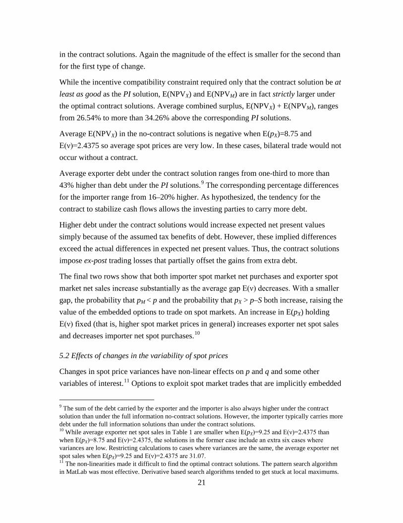
Average exporter debt under the contract solution ranges from one-third to more than 43% higher than debt under the PI solutions.9 The corresponding percentage differences for the importer range from 16–20% higher. As hypothesized, the tendency for the contract to stabilize cash flows allows the investing parties to carry more debt.

Higher debt under the contract solutions would increase expected net present values simply because of the assumed tax benefits of debt. However, these implied differences exceed the actual differences in expected net present values. Thus, the contract solutions impose ex-post trading losses that partially offset the gains from extra debt.

The final two rows show that both importer spot market net purchases and exporter spot market net sales increase substantially as the average gap E(ν) decreases. With a smaller gap, the probability that pM < p and the probability that pX > p–S both increase, raising the value of the embedded options to trade on spot markets. An increase in E(pX) holding E(ν) fixed (that is, higher spot market prices in general) increases exporter net spot sales and decreases importer net spot purchases.10

5.2 Effects of changes in the variability of spot prices

Changes in spot price variances have non-linear effects on p and q and some other variables of interest.11 Options to exploit spot market trades that are implicitly embedded

9 The sum of the debt carried by the exporter and the importer is also always higher under the contract solution than under the full information no-contract solutions. However, the importer typically carries more debt under the full information solutions than under the contract solutions. 10 While average exporter net spot sales in Table 1 are smaller when E(pX)=9.25 and E(ν)=2.4375 than when E(pX)=8.75 and E(ν)=2.4375, the solutions in the former case include an extra six cases where variances are low. Restricting calculations to cases where variances are the same, the average exporter net spot sales when E(pX)=9.25 and E(ν)=2.4375 are 31.07. 11 The non-linearities made it difficult to find the optimal contract solutions. The pattern search algorithm in MatLab was most effective. Derivative based search algorithms tended to get stuck at local maximums.

21

in the contract are affected non-linearly by changes in spot price variances, as are the values of any efficient ex-post trades precluded by the contract. In addition, increased spot price variability raises cash flow variability, thereby increasing the leverage benefits of the contract.

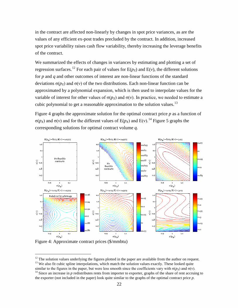
We summarized the effects of changes in variances by estimating and plotting a set of regression surfaces.12 For each pair of values for E(pX) and E(ν), the different solutions for p and q and other outcomes of interest are non-linear functions of the standard deviations σ(pX) and σ(ν) of the two distributions. Each non-linear function can be approximated by a polynomial expansion, which is then used to interpolate values for the variable of interest for other values of σ(pX) and σ(ν). In practice, we needed to estimate a cubic polynomial to get a reasonable approximation to the solution values.13

Figure 4 graphs the approximate solution for the optimal contract price p as a function of σ(pX) and σ(ν) and for the different values of E(pX) and E(ν).14 Figure 5 graphs the corresponding solutions for optimal contract volume q.

Figure 4: Approximate contract prices ($/mmbtu)

12 The solution values underlying the figures plotted in the paper are available from the author on request. 13 We also fit cubic spline interpolations, which match the solution values exactly. These looked quite similar to the figures in the paper, but were less smooth since the coefficients vary with σ(pX) and σ(ν). 14 Since an increase in p redistributes rents from importer to exporter, graphs of the share of rent accruing to the exporter (not included in the paper) look quite similar to the graphs of the optimal contract price p.

22

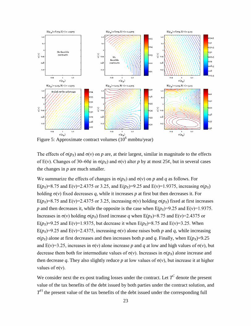
Figure 5: Approximate contract volumes (106 mmbtu/year)

The effects of σ(pX) and σ(ν) on p are, at their largest, similar in magnitude to the effects of E(ν). Changes of 30–60¢ in σ(pX) and σ(ν) alter p by at most 25¢, but in several cases the changes in p are much smaller.

We summarize the effects of changes in σ(pX) and σ(ν) on p and q as follows. For E(pX)=8.75 and E(ν)=2.4375 or 3.25, and E(pX)=9.25 and E(ν)=1.9375, increasing σ(pX) holding σ(ν) fixed decreases q, while it increases p at first but then decreases it. For E(pX)=8.75 and E(ν)=2.4375 or 3.25, increasing σ(ν) holding σ(pX) fixed at first increases p and then decreases it, while the opposite is the case when E(pX)=9.25 and E(ν)=1.9375. Increases in σ(ν) holding σ(pX) fixed increase q when E(pX)=8.75 and E(ν)=2.4375 or E(pX)=9.25 and E(ν)=1.9375, but decrease it when E(pX)=8.75 and E(ν)=3.25. When E(pX)=9.25 and E(ν)=2.4375, increasing σ(ν) alone raises both p and q, while increasing σ(pX) alone at first decreases and then increases both p and q. Finally, when E(pX)=9.25 and E(ν)=3.25, increases in σ(ν) alone increase p and q at low and high values of σ(ν), but decrease them both for intermediate values of σ(ν). Increases in σ(pX) alone increase and then decrease q. They also slightly reduce p at low values of σ(ν), but increase it at higher values of σ(ν).

We consider next the ex-post trading losses under the contract. Let TC denote the present value of the tax benefits of the debt issued by both parties under the contract solution, and TFI the present value of the tax benefits of the debt issued under the corresponding full

23

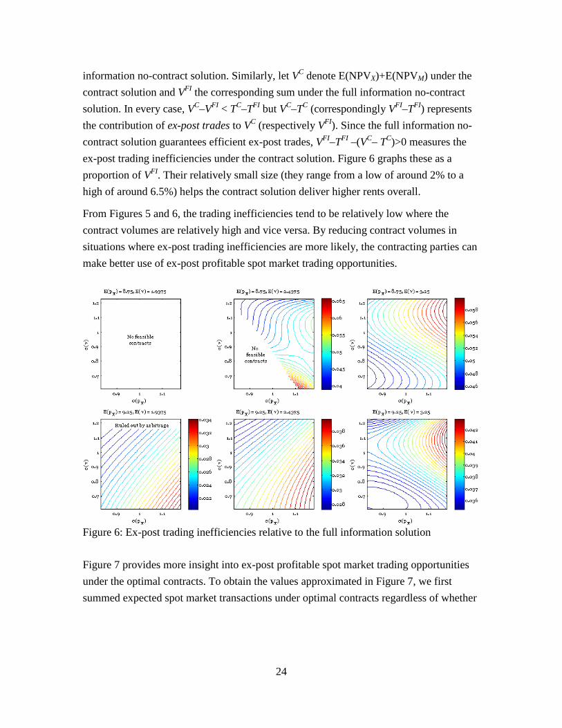
information no-contract solution. Similarly, let VC denote E(NPVX)+E(NPVM) under the contract solution and VFI the corresponding sum under the full information no-contract solution. In every case, VC–VFI < TC–TFI but VC–TC (correspondingly VFI–TFI) represents the contribution of ex-post trades to VC (respectively VFI). Since the full information no-contract solution guarantees efficient ex-post trades, VFI–TFI –(VC– TC)>0 measures the ex-post trading inefficiencies under the contract solution. Figure 6 graphs these as a proportion of VFI. Their relatively small size (they range from a low of around 2% to a high of around 6.5%) helps the contract solution deliver higher rents overall.

From Figures 5 and 6, the trading inefficiencies tend to be relatively low where the contract volumes are relatively high and vice versa. By reducing contract volumes in situations where ex-post trading inefficiencies are more likely, the contracting parties can make better use of ex-post profitable spot market trading opportunities.

Figure 6: Ex-post trading inefficiencies relative to the full information solution

Figure 7 provides more insight into ex-post profitable spot market trading opportunities under the optimal contracts. To obtain the values approximated in Figure 7, we first summed expected spot market transactions under optimal contracts regardless of whether

24

they are a sale or purchase, and regardless of the whether the transacting party is the exporter or the importer.15 We then divided that result by the optimal contract volume.

Figure 7: Gross spot market transactions relative to contracted volumes

Figure 8: Additional exporter plus importer debt under the contract solutions

15 The graphs of spot net sales by the exporter looked very similar to Figure 7, while spot net purchases by the importer looked like the graphs in Figure 7 slightly rotated in the counter-clockwise direction. For E(pX)=9.25, E(ν)=3.25, the importer spot net purchases graph was also translated to the right.

25

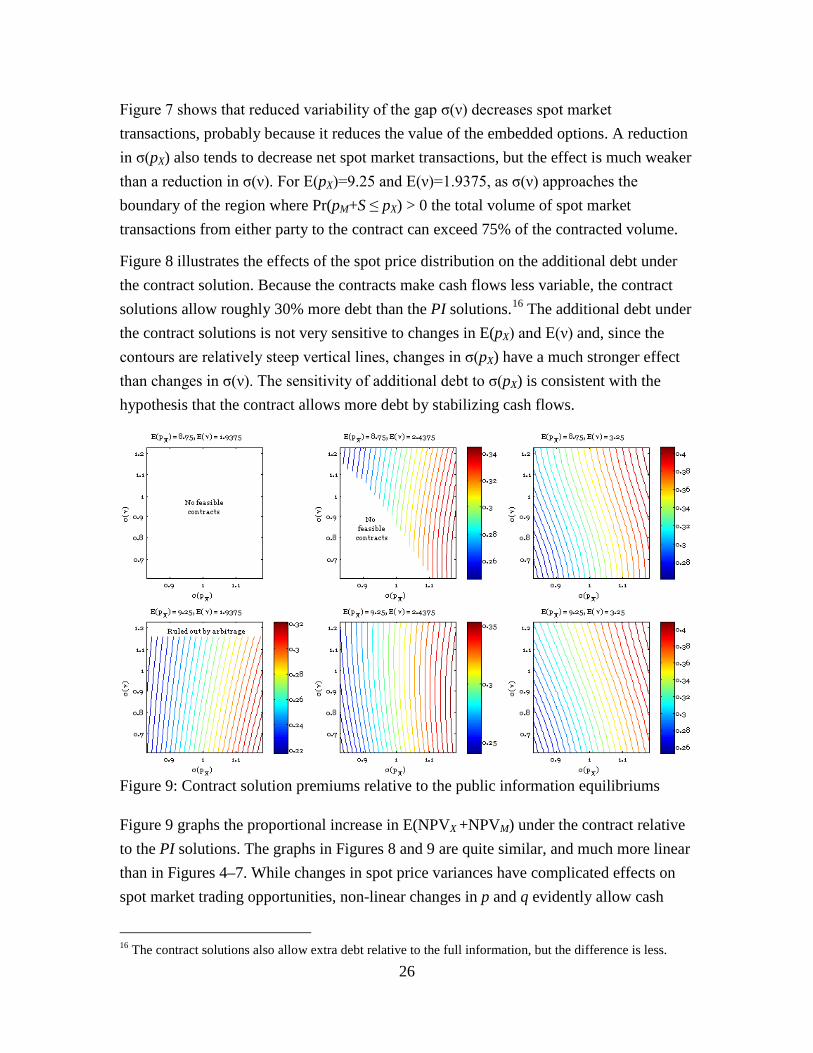
Figure 7 shows that reduced variability of the gap σ(ν) decreases spot market transactions, probably because it reduces the value of the embedded options. A reduction in σ(pX) also tends to decrease net spot market transactions, but the effect is much weaker than a reduction in σ(ν). For E(pX)=9.25 and E(ν)=1.9375, as σ(ν) approaches the boundary of the region where Pr(pM+S ≤ pX) > 0 the total volume of spot market transactions from either party to the contract can exceed 75% of the contracted volume.

Figure 8 illustrates the effects of the spot price distribution on the additional debt under the contract solution. Because the contracts make cash flows less variable, the contract solutions allow roughly 30% more debt than the PI solutions.16 The additional debt under the contract solutions is not very sensitive to changes in E(pX) and E(ν) and, since the contours are relatively steep vertical lines, changes in σ(pX) have a much stronger effect than changes in σ(ν). The sensitivity of additional debt to σ(pX) is consistent with the hypothesis that the contract allows more debt by stabilizing cash flows.

Figure 9: Contract solution premiums relative to the public information equilibriums

Figure 9 graphs the proportional increase in E(NPVX +NPVM) under the contract relative to the PI solutions. The graphs in Figures 8 and 9 are quite similar, and much more linear than in Figures 4–7. While changes in spot price variances have complicated effects on spot market trading opportunities, non-linear changes in p and q evidently allow cash

16 The contract solutions also allow extra debt relative to the full information, but the difference is less.

26

flows to change much more linearly in response to changes in σ(pX) and σ(ν). As a result, the additional debt afforded by a contract also changes more linearly.17

The contract solution yields on average around 30% higher surplus than the corresponding PI solution.18 The advantage of a contract is not much affected by the general level E(pX) of spot market prices, but reducing the average gap E(ν) between pM and pX noticeably reduces the benefits of a contract. Figure 9 also reveals that a decrease in σ(pX) substantially reduces the benefits of a contract, but the effect of σ(ν) is weak and generally more ambiguous. Comparing Figures 8 and 9, the key reason for reduced benefits of a contract as σ(pX) declines is that reduced variability of spot prices also reduces the extra debt under a contract.

In summary, the contract solutions yield a higher joint expected net present value for the participants predominantly because they allow for increased debt finance. Inefficiencies arising from contract limitations on spot market trading are not large, with changes in contract terms and supplemental spot market trades helping limit them. A smaller gap between average spot prices available to the exporter and the importer, and lower variability of spot market prices, reduces the advantages of a contract. A smaller gap between average importer and exporter spot market prices also encourages substantially more spot market trading by parties to the contract. On the other hand, a decrease in the variability of the gap between importer and exporter prices tends to decrease the amount of spot trading by parties to a contract.

5.3 Effects of increasing spot market liquidity

As observed in Section 2, the LNG market has recently become considerably more liquid. The numbers of available buyers and sellers have increased, spot and short-term trading has grown, and prices for spot and short-term trades have become less sensitive to individual trades. Increased liquidity should, in turn, reduce the variability of spot prices, denoted σ(pX) in the model.

Entry by new suppliers and demanders also reduces the average distance between any two potential trading partners. This will in turn tend to reduce the gap between average spot prices available to exporters and importers, characterized as E(ν) in the model.

17 The cubic approximations in Figures 8 and 9 also fit the calculated values much more accurately. 18 The numerical results also reveal that E(NPVX + NPVM) under the contract solutions is approximately 12% higher than the corresponding sum under the spot market solutions based on all full information.

27

From the above analysis, reducing both σ(pX) and E(ν) would reduce the superiority of long-term contracts relative to short-term and spot trading. At the same time, reducing E(ν) would greatly increase the amount of spot market trading from parties to existing contracts. Although a simultaneous reduction in σ(ν) would tend to have the opposite effect, the results in Figure 7 suggest that the change in E(ν) is likely to dominate.

6. Concluding comments

As more firms import LNG, and more producers enter the market, the average difference between spot market prices available to an importer and netback prices available to an exporter will decline. The overall elasticity of supply or demand facing any one party also will tend to increase. The use of natural gas in a wider range of applications may also raise demand elasticities. At the same time, more firms are positioning themselves to take advantage of geographic and intertemporal LNG price differentials. Examples discussed in section 2 include proposed US export terminals collocated with regasification and storage facilities, the flexible portfolio approach to LNG trading by BG and the Singapore and National Grid LNG storage facilities. As a result of these developments, spot market prices are likely to become less variable over time.

The model presented in this paper suggests that these developments will erode the advantages of long-term contracts in allowing higher project leverage. At the same time, the changes are likely to increase spot market participation by parties under contract, further raising spot market liquidity. An increased desire to take advantage of spot and short-term arbitrage opportunities should also raise the demand for greater flexibility in long-term contracts. Accordingly, we can foresee continuing evolution of world LNG markets toward a larger proportion of volumes being traded on short-term contracts or sold as spot cargoes, and increased use of swaps, re-exports and other similar short-term arrangements taking advantage of temporary arbitrage opportunities.

7. References

Brito, Dagobert and Peter Hartley (2007). “Expectations and the Evolving World Gas Market,” The Energy Journal, 28(1): 1–24.

Canes, Michael E. and Donald A. Norman (1984). “Long-Term Contracts and Market Forces in the Natural Gas Market,” The Journal of Energy and Development 10(1): 73–96.

Creti, Anna and Villeneuve, Bertrand (2005). “Long-term Contracts and Take-or-Pay Clauses in Natural Gas Markets,” Energy Studies Review 13(1): 75–94.

28

Crocker, Keith J. and Scott E. Masten (1988). “Mitigating Contractual Hazards: Unilateral Options and Contract Length,” The RAND Journal of Economics, 19(3): 327–343

Hirschhausen, Christian von and Anne Neumann (2008). “Long-Term Contracts and Asset Specificity Revisited: An Empirical Analysis of Producer-Importer Relations in the Natural Gas Industry,” Review of Industrial Organization 32(2): 131-143

International Gas Union (2009). “2006-2009 Triennium Work Report, Programme Committee D Study Group 2, LNG, Chapter 3: LNG Contracts” presented to the International Gas Union 24th World Gas Conference, Argentina, and available at http://www.igu.org/html/wgc2009/committee/PGCD/PGCD_Study_Group_2_Report.pdf

Masten, Scott E. and Keith J. Crocker (1985). “Efficient Adaptation in Long-Term Contracts: Take-or-Pay Provisions for Natural Gas,” American Economic Review 75(5): 1083-1093.

Ruester, Sophia (2009). “Changing Contract Structures in the International Liquefied Natural Gas Market – A First Empirical Analysis,” Revue D’Économie Industrielle 127(3): 89–112.

Thompson, Stephen (2009). “The New LNG Trading Model: Short-Term Market Developments and Prospects,” Poten & Partners, Inc., paper presented to the International Gas Union 24th World Gas Conference, Argentina, available at http://www.igu.org/html/wgc2009/papers/docs/wgcFinal00351.pdf

Williamson, Oliver E. (1979). “Transaction-Cost Economics: The Governance of Contractual Relations,” Journal of Law and Economics, 22(2): 233–261.

29

Editor, UWA Economics Discussion Papers: Ernst Juerg Weber Business School – Economics University of Western Australia 35 Sterling Hwy Crawley WA 6009 Australia Email: ecoadmin@biz.uwa.edu.au The Economics Discussion Papers are available at: 1980 – 2002: http://ecompapers.biz.uwa.edu.au/paper/PDF%20of%20Discussion%20Papers/ Since 2001: http://ideas.repec.org/s/uwa/wpaper1.html Since 2004: http://www.business.uwa.edu.au/school/disciplines/economics

ECONOMICS DISCUSSION PAPERS 2011

DP NUMBER AUTHORS TITLE

11.01 Robertson, P.E. DEEP IMPACT: CHINA AND THE WORLD ECONOMY

11.02 Kang, C. and Lee, S.H. BEING KNOWLEDGEABLE OR SOCIABLE? DIFFERENCES IN RELATIVE IMPORTANCE OF COGNITIVE AND NON-COGNITIVE SKILLS

11.03 Turkington, D. DIFFERENT CONCEPTS OF MATRIX CALCULUS

11.04 Golley, J. and Tyers, R. CONTRASTING GIANTS: DEMOGRAPHIC CHANGE AND ECONOMIC PERFORMANCE IN CHINA AND INDIA

11.05 Collins, J., Baer, B. and Weber, E.J. ECONOMIC GROWTH AND EVOLUTION: PARENTAL PREFERENCE FOR QUALITY AND QUANTITY OF OFFSPRING

11.06 Turkington, D. ON THE DIFFERENTIATION OF THE LOG LIKELIHOOD FUNCTION USING MATRIX CALCULUS

11.07 Groenewold, N. and Paterson, J.E.H. STOCK PRICES AND EXCHANGE RATES IN AUSTRALIA: ARE COMMODITY PRICES THE MISSING LINK?

11.08 Chen, A. and Groenewold, N. REDUCING REGIONAL DISPARITIES IN CHINA: IS INVESTMENT ALLOCATION POLICY EFFECTIVE?

11.09 Williams, A., Birch, E. and Hancock, P. THE IMPACT OF ON-LINE LECTURE RECORDINGS ON STUDENT PERFORMANCE

11.10 Pawley, J. and Weber, E.J. INVESTMENT AND TECHNICAL PROGRESS IN THE G7 COUNTRIES AND AUSTRALIA

11.11 Tyers, R. AN ELEMENTAL MACROECONOMIC MODEL FOR APPLIED ANALYSIS AT UNDERGRADUATE LEVEL

30

11.12 Clements, K.W. and Gao, G. QUALITY, QUANTITY, SPENDING AND PRICES

11.13 Tyers, R. and Zhang, Y. JAPAN’S ECONOMIC RECOVERY: INSIGHTS FROM MULTI-REGION DYNAMICS

11.14 McLure, M. A. C. PIGOU’S REJECTION OF PARETO’S LAW

11.15 Kristoffersen, I. THE SUBJECTIVE WELLBEING SCALE: HOW REASONABLE IS THE CARDINALITY ASSUMPTION?

11.16 Clements, K.W., Izan, H.Y. and Lan, Y. VOLATILITY AND STOCK PRICE INDEXES

11.17 Parkinson, M. SHANN MEMORIAL LECTURE 2011: SUSTAINABLE WELLBEING – AN ECONOMIC FUTURE FOR AUSTRALIA

11.18 Chen, A. and Groenewold, N. THE NATIONAL AND REGIONAL EFFECTS OF FISCAL DECENTRALISATION IN CHINA

11.19 Tyers, R. and Corbett, J. JAPAN’S ECONOMIC SLOWDOWN AND ITS GLOBAL IMPLICATIONS: A REVIEW OF THE ECONOMIC MODELLING

11.20 Wu, Y. GAS MARKET INTEGRATION: GLOBAL TRENDS AND IMPLICATIONS FOR THE EAS REGION

11.21 Fu, D., Wu, Y. and Tang, Y. DOES INNOVATION MATTER FOR CHINESE HIGH-TECH EXPORTS? A FIRM-LEVEL ANALYSIS

11.22 Fu, D. and Wu, Y. EXPORT WAGE PREMIUM IN CHINA’S MANUFACTURING SECTOR: A FIRM LEVEL ANALYSIS

11.23 Li, B. and Zhang, J. SUBSIDIES IN AN ECONOMY WITH ENDOGENOUS CYCLES OVER NEOCLASSICAL INVESTMENT AND NEO-SCHUMPETERIAN INNOVATION REGIMES

11.24 Krey, B., Widmer, P.K. and Zweifel, P. EFFICIENT PROVISION OF ELECTRICITY FOR THE UNITED STATES AND SWITZERLAND

11.25 Wu, Y. ENERGY INTENSITY AND ITS DETERMINANTS IN CHINA’S REGIONAL ECONOMIES

31

ECONOMICS DISCUSSION PAPERS 2012

DP NUMBER AUTHORS TITLE

12.01 Clements, K.W., Gao, G., and Simpson, T.

DISPARITIES IN INCOMES AND PRICES INTERNATIONALLY

12.02 Tyers, R. THE RISE AND ROBUSTNESS OF ECONOMIC FREEDOM IN CHINA

12.03 Golley, J. and Tyers, R. DEMOGRAPHIC DIVIDENDS, DEPENDENCIES AND ECONOMIC GROWTH IN CHINA AND INDIA

12.04 Tyers, R. LOOKING INWARD FOR GROWTH

12.05 Knight, K. and McLure, M. THE ELUSIVE ARTHUR PIGOU

12.06 McLure, M. ONE HUNDRED YEARS FROM TODAY: A. C. PIGOU’S WEALTH AND WELFARE

12.07 Khuu, A. and Weber, E.J. HOW AUSTRALIAN FARMERS DEAL WITH RISK

12.08 Chen, M. and Clements, K.W. PATTERNS IN WORLD METALS PRICES

12.09 Clements, K.W. UWA ECONOMICS HONOURS

12.10 Golley, J. and Tyers, R. CHINA’S GENDER IMBALANCE AND ITS ECONOMIC PERFORMANCE

12.11 Weber, E.J. AUSTRALIAN FISCAL POLICY IN THE AFTERMATH OF THE GLOBAL FINANCIAL CRISIS

12.12 Hartley, P.R. and Medlock III, K.B. CHANGES IN THE OPERATIONAL EFFICIENCY OF NATIONAL OIL COMPANIES

12.13 Li, L. HOW MUCH ARE RESOURCE PROJECTS WORTH? A CAPITAL MARKET PERSPECTIVE

12.14 Chen, A. and Groenewold, N. THE REGIONAL ECONOMIC EFFECTS OF A REDUCTION IN CARBON EMISSIONS AND AN EVALUATION OF OFFSETTING POLICIES IN CHINA

12.15 Collins, J., Baer, B. and Weber, E.J. SEXUAL SELECTION, CONSPICUOUS CONSUMPTION AND ECONOMIC GROWTH

12.16 Wu, Y. TRENDS AND PROSPECTS IN CHINA’S R&D SECTOR

12.17 Cheong, T.S. and Wu, Y. INTRA-PROVINCIAL INEQUALITY IN CHINA: AN ANALYSIS OF COUNTY-LEVEL DATA

12.18 Cheong, T.S. THE PATTERNS OF REGIONAL INEQUALITY IN CHINA

12.19 Wu, Y. ELECTRICITY MARKET INTEGRATION: GLOBAL TRENDS AND IMPLICATIONS FOR THE EAS REGION

12.20 Knight, K. EXEGESIS OF DIGITAL TEXT FROM THE HISTORY OF ECONOMIC THOUGHT: A COMPARATIVE EXPLORATORY TEST

12.21 Chatterjee, I. COSTLY REPORTING, EX-POST MONITORING, AND COMMERCIAL PIRACY: A GAME THEORETIC ANALYSIS

32

12.22 Pen, S.E. QUALITY-CONSTANT ILLICIT DRUG PRICES

12.23 Cheong, T.S. and Wu, Y. REGIONAL DISPARITY, TRANSITIONAL DYNAMICS AND CONVERGENCE IN CHINA

12.24 Ezzati, P. FINANCIAL MARKETS INTEGRATION OF IRAN WITHIN THE MIDDLE EAST AND WITH THE REST OF THE WORLD

12.25 Kwan, F., Wu, Y. and Zhuo, S. RE-EXAMINATION OF THE SURPLUS AGRICULTURAL LABOUR IN CHINA

12.26 Wu, Y. R&D BEHAVIOUR IN CHINESE FIRMS

12.27 Tang, S.H.K. and Yung, L.C.W. MAIDS OR MENTORS? THE EFFECTS OF LIVE-IN FOREIGN DOMESTIC WORKERS ON SCHOOL CHILDREN’S EDUCATIONAL ACHIEVEMENT IN HONG KONG

12.28 Groenewold, N. AUSTRALIA AND THE GFC: SAVED BY ASTUTE FISCAL POLICY?

ECONOMICS DISCUSSION PAPERS 2013

DP NUMBER AUTHORS TITLE

13.01 Chen, M., Clements, K.W. and Gao, G.

THREE FACTS ABOUT WORLD METAL PRICES

13.02 Collins, J. and Richards, O. EVOLUTION, FERTILITY AND THE AGEING POPULATION

13.03 Clements, K., Genberg, H., Harberger, A., Lothian, J., Mundell, R., Sonnenschein, H. and Tolley, G.

LARRY SJAASTAD, 1934-2012

13.04 Robitaille, M.C. and Chatterjee, I. MOTHERS-IN-LAW AND SON PREFERENCE IN INDIA

13.05 Clements, K.W. and Izan, I.H.Y. REPORT ON THE 25TH PHD CONFERENCE IN ECONOMICS AND BUSINESS

13.06 Walker, A. and Tyers, R. QUANTIFYING AUSTRALIA’S “THREE SPEED” BOOM

13.07 Yu, F. and Wu, Y. PATENT EXAMINATION AND DISGUISED PROTECTION

13.08 Yu, F. and Wu, Y. PATENT CITATIONS AND KNOWLEDGE SPILLOVERS: AN ANALYSIS OF CHINESE PATENTS REGISTER IN THE US

13.09 Chatterjee, I. and Saha, B. BARGAINING DELEGATION IN MONOPOLY

13.10 Cheong, T.S. and Wu, Y. GLOBALIZATION AND REGIONAL INEQUALITY IN CHINA

13.11 Cheong, T.S. and Wu, Y. INEQUALITY AND CRIME RATES IN CHINA

13.12 Robertson, P.E. and Ye, L. ON THE EXISTENCE OF A MIDDLE INCOME TRAP

33

13.13 Robertson, P.E. THE GLOBAL IMPACT OF CHINA’S GROWTH

13.14 Hanaki, N., Jacquemet, N., Luchini, S., and Zylbersztejn, A.

BOUNDED RATIONALITY AND STRATEGIC UNCERTAINTY IN A SIMPLE DOMINANCE SOLVABLE GAME

13.15 Okatch, Z., Siddique, A. and Rammohan, A.

DETERMINANTS OF INCOME INEQUALITY IN BOTSWANA

13.16 Clements, K.W. and Gao, G. A MULTI-MARKET APPROACH TO MEASURING THE CYCLE

13.17 Chatterjee, I. and Ray, R. THE ROLE OF INSTITUTIONS IN THE INCIDENCE OF CRIME AND CORRUPTION

13.18 Fu, D. and Wu, Y. EXPORT SURVIVAL PATTERN AND DETERMINANTS OF CHINESE MANUFACTURING FIRMS

13.19 Shi, X., Wu, Y. and Zhao, D. KNOWLEDGE INTENSIVE BUSINESS SERVICES AND THEIR IMPACT ON INNOVATION IN CHINA

13.20 Tyers, R., Zhang, Y. and Cheong, T.S.

CHINA’S SAVING AND GLOBAL ECONOMIC PERFORMANCE

13.21 Collins, J., Baer, B. and Weber, E.J. POPULATION, TECHNOLOGICAL PROGRESS AND THE EVOLUTION OF INNOVATIVE POTENTIAL

13.22 Hartley, P.R. THE FUTURE OF LONG-TERM LNG CONTRACTS

13.23 Tyers, R. A SIMPLE MODEL TO STUDY GLOBAL MACROECONOMIC INTERDEPENDENCE

13.24 McLure, M. REFLECTIONS ON THE QUANTITY THEORY: PIGOU IN 1917 AND PARETO IN 1920-21

34