Economics of Digitization Munich, 22–23 November 2019

How Does Competition Affect Reputation

Concerns? Theory and Evidence from Airbnb Michelangelo Rossi 

How Does Competition A�ect Reputation Concerns?

Theory and Evidence from Airbnb*

Michelangelo Rossi�

November 9, 2019

(click here for the latest version)

Abstract

I show how changes in competition a�ect the power of reputation to induce sellers to exert

e�ort. The impact of competition on sellers' incentives is theoretically ambiguous. More com-

petition disciplines sellers, but, at the same time, it erodes reputational premia. This paper

identi�es empirically whether one e�ect dominates the other using data from Airbnb. To guide

the empirical analysis, I develop a model of reputation where the relative number of hosts

and guests a�ects the value of building a reputation through e�ort. In this framework, more

competition depresses hosts' pro�ts and leads hosts to reduce e�ort. I test the model's predic-

tion exploiting a change in regulation for Airbnb listings e�ective in San Francisco in 2017. I

identify a negative causal e�ect of competition on e�ort. As the number of competitors sur-

rounding each listing increases by 10 percent, ratings about hosts' e�ort decrease by more than

one standard deviation. These �ndings suggest that more competition may erode incentives

for high-quality services in markets where sellers' performances depend on reputation.

JEL codes: D82, D83, L50, L81.

Keywords: Reputation, Competition, Digitization.

*I am grateful to my advisors, Natalia Fabra and Matilde Pinto Machado, for their patient guidance and advice.I also thank Victor Aguirregabiria, Heski Bar-Isaac, Jesús Carro, Ambarish Chandra, Rahul Deb, Alexandre deCornière, Daniel Ershov, Chiara Farronato, Alberto Galasso, Ignatius J. Horstmann, Bruno Jullien, Gerard Llobet,Luigi Minale, Matthew Mitchell, Maryam Saeedi, Jan Stuhler, Mark Tremblay, and Gabor Virag. Helpful feed-back was received at the internal seminars at Universidad Carlos III de Madrid, CEMFI, and Rotman School ofManagement, at the International Industrial Organization Conference, the Doctoral Workshop on The Economics ofDigitization, the CEPR/JIE School on Applied Industrial Organisation, the European Association Research Indus-trial Economics Conference, the Jornadas de Economia Industrial, and the TSE Digital Workshop. Special gratitudeto Elizaveta Pronkina for her enormous support and encouragement. All errors are mine. Support from the MinisterioEconomía, Industria y Competitividad (Spain), grant ECO2016/78632-P, is gratefully acknowledged.

�Universidad Carlos III, Department of Economics, Madrid, Spain. E-mail: mrossi@eco.uc3m.es.

1

1 Introduction

The rise of online marketplaces had a strong impact on many industries in the last decade. Thanks

to their low entry costs, these platforms facilitate the entry of new service providers. As an example,

in the last years Airbnb hosts massively entered the hospitality market and now they outnumber

the largest hotel chains in terms of available rooms: in 2019, there are more than seven million

Airbnb listings around the world. For comparison, the Marriott chain has less than 1.5 million

rooms.1 Digital platforms rely on review systems to ensure the quality of their services and to

provide incentives for sellers to exert e�ort. Reviews reveal sellers' past performances and form

their reputation. Thus, sellers' concerns for a good reputation are one of the key ingredients for the

quality of online transactions and the success of digital marketplaces.

This paper studies how changes in the number of competitors a�ect the power of reputation

to provide incentives for sellers to exert e�ort. The e�ects of competition on the sellers' incentives

are theoretically ambiguous (Bar-Isaac, 2005). More competition may help to discipline sellers, but,

at the same time, it erodes reputational premia. Understanding which of the two e�ects dominates

empirically is a relevant question, not only for the design of digital platforms, but also for other

markets in which sellers' quality is unknown and their performances depend on reputation. This

feature is common to several markets involving experience goods and services such as hospitals,

restaurants, or schools. Yet, the process of reputation building is particularly relevant in online

marketplaces since review systems provide an observable measure of sellers' reputation and e�ort.

I empirically address this research question using data from one of the fastest-growing online

platforms: Airbnb. This setting is of special interest since the enormous growth in the number of

hosts on the platform has attracted considerable attention from local governments and regulators.

Previous works have shown that the entry of Airbnb hosts in a city expands the number of available

rooms, reduces hotels' pro�ts, and increases consumers' welfare (Zervas et al., 2017; and Farronato

and Fradkin, 2018). Yet, in addition to the disciplining impact of competition on prices, an increase

in the number of competitors may also impact hosts' incentives to exert e�ort a�ecting the quality

of platform's services. To the best of my knowledge, this is the �rst paper to identify the causal

impact of the number of competitors on the incentives to exert e�ort in online marketplaces: my

�ndings show that, when the number of competitors increases, hosts exert less e�ort and their

pro�ts reduce.

To inform my empirical analysis, I develop a model of reputation in which the number of

hosts and guests on the two sides of the market (the market tightness) impacts the reputation

return of hosts' e�ort. The model predicts that, when the number of competitors decreases, hosts'

1For more information about the recent growth of Airbnb around the world, see the annual o�cial reports providedby Airbnb at https://press.airbnb.com/fast-facts/.

2

pro�ts increase and hosts exert more e�ort. With fewer competitors, hosts have higher probability

to be matched with a guest and can charge higher prices. However, the price elasticity of hosts'

demand depends on their reputation. In particular, the probability to be matched with a guest is

less elastic for hosts with good reputation. Accordingly, the premium of exerting e�ort (and having

good reputation) increases when the number of competitors is lower: hosts with good reputation

can post higher prices with a lower reduction in their demand.

In order to test the model's prediction, I analyze empirically the relationship between the

e�ort exerted by Airbnb hosts and the number of their competitors. I measure hosts' e�ort by

studying ratings such as communication and check-in that are speci�cally related to hosts' actions.

Moreover, to measure the number of competitors for each host, I create host-speci�c consideration

sets by counting the number of listings surrounding each host within a radius of 0.5, 1, and 2

kilometers. Doing so, I assume that Airbnb hosts compete more strongly with listings that are

closely located to them, relative to those further away. This is in line with Zervas et al. (2017) who

show that the impact of Airbnb entry on hotels' revenues is sensitive to the distance between hotels

and Airbnb listings.

My identi�cation strategy exploits a unique quasi-experiment to isolate the e�ect of changes in

the number of competitors from other confounders. In particular, I take advantage of a regulatory

enforcement on short-term rentals that occurred in San Francisco in 2017.

Airbnb was founded in San Francisco. In 2015, it was the third US city in terms of active

Airbnb listings after New York and Los Angeles (Lane et al., 2016). From that year, the San

Francisco City Council imposed several restrictions and a formal registration for short-term rentals

on digital platforms.2 Yet, the regulation started to be e�ectively enforced only two years later,

when Airbnb signed a Settlement Agreement with the City Council in May 2017. Accordingly, the

platform has been actively engaged in the listings' registration process since September 2017. As

shown in Figure 1, the percentage of Airbnb listings o�ering short-term lodging formally registered

at the City Council O�ce dramatically increased from less than 15 percent in September 2017 to 100

percent in February 2018: hosts started to register, and those who could not, exited the platform.

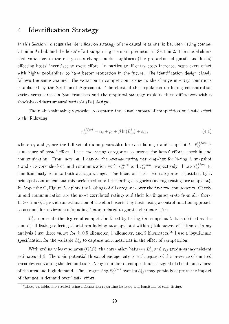
As a result, a few months after September 2017, the number of Airbnb listings o�ering short-term

lodging halved, dropping from about 8,000 units in September 2017 to less than 4,000 in February

2018 (see Figure 2).

I exploit this regulatory enforcement as an exogenous shift in the number of listings surround-

ing each host. I focus on hosts renting short-term that were present on the platform both before

and after the Settlement Agreement. By such selection, I abstract from hosts' decision to enter or

exit due to the regulation enforcement. All hosts renting short-term in San Francisco are a�ected

2Rentals are considered �short-term� if the properties are rented for less than 30 consecutive nights at a time.

3

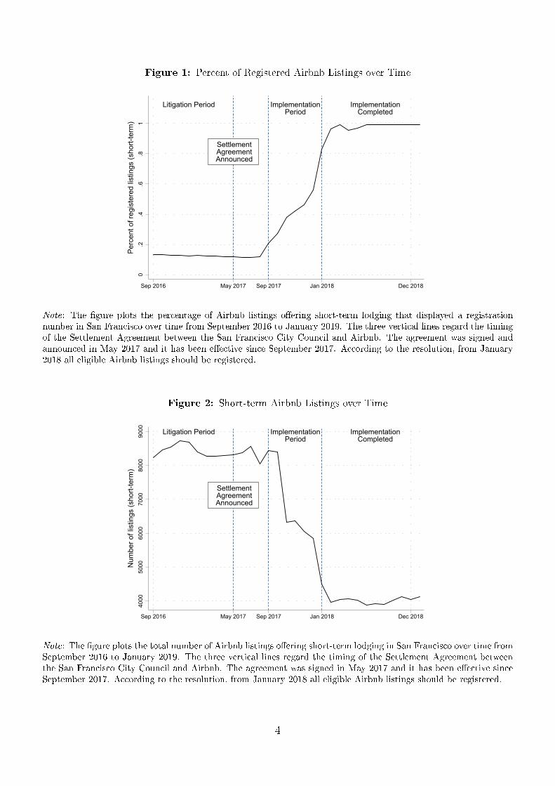
Figure 1: Percent of Registered Airbnb Listings over Time

Litigation Period

SettlementAgreementAnnounced

ImplementationPeriod

ImplementationCompleted

0.2

.4.6

.81

Perc

ent o

f reg

iste

red

listin

gs (s

hort-

term

)

Sep 2016 May 2017 Sep 2017 Jan 2018 Dec 2018

Note: The �gure plots the percentage of Airbnb listings o�ering short-term lodging that displayed a registrationnumber in San Francisco over time from September 2016 to January 2019. The three vertical lines regard the timingof the Settlement Agreement between the San Francisco City Council and Airbnb. The agreement was signed andannounced in May 2017 and it has been e�ective since September 2017. According to the resolution, from January2018 all eligible Airbnb listings should be registered.

Figure 2: Short-term Airbnb Listings over Time

Litigation Period

SettlementAgreementAnnounced

ImplementationPeriod

ImplementationCompleted

4000

5000

6000

7000

8000

9000

Num

ber o

f lis

tings

(sho

rt-te

rm)

Sep 2016 May 2017 Sep 2017 Jan 2018 Dec 2018

Note: The �gure plots the total number of Airbnb listings o�ering short-term lodging in San Francisco over time fromSeptember 2016 to January 2019. The three vertical lines regard the timing of the Settlement Agreement betweenthe San Francisco City Council and Airbnb. The agreement was signed in May 2017 and it has been e�ective sinceSeptember 2017. According to the resolution, from January 2018 all eligible Airbnb listings should be registered.

4

by the Settlement Agreement. On the other hand, the exposure to this �shock� di�ers since the

variation in the number of competitors is heterogeneous across hosts. I take advantage of this

heterogeneity in the treatment. To measure the exposure of each host, I use the percentage of

listings surrounding each host that were already registered in September 2017. For higher values

of this percentage, fewer listings are likely to exit after the Settlement Agreement since they were

already complying with the regulation. I employ this measure as a predictor for the variation in the

number of listings surrounding each host after the Settlement Agreement. Therefore, I identify the

e�ect of variations in the number of competitors by using the di�erential changes in the exposure

across listings over time. The core identifying assumption of this design shares the intuition of a

di�erence in di�erences estimator with a continuous treatment. However, the identi�cation s based

on an instrumental variable regression where the excluded instrument is given by the interaction

between the measure of exposure (the percentage of listings already registered in September 2017)

and time.

The results show a statistically and economically signi�cant negative relationship between

the number of competitors and hosts' e�ort. When the number of competitors decreases by 10%,

ratings regarding hosts' e�ort increase by more than one standard deviation. I corroborate this

result studying variations in hosts' pro�ts and in the monetary value of reputation. With the

same identi�cation strategy, I �nd that less competition increases pro�ts, so that hosts have higher

incentives to exert e�ort. Moreover, since fewer hosts are going to have good reputation, I show

evidence that the signaling e�ect of reputation is stronger in more competitive frameworks.

This paper makes contributions to both the empirical and theoretical literatures on reputation.

To the best of my knowledge, there are no studies that investigate empirically the relationship

between competition and sellers' reputational incentives to exert e�ort. The empirical literature

about reputation has grown in past years with a particular focus on online settings. Still, the

majority of the empirical papers study the impact of online feedback on sellers' pro�ts and they do

not specify the mechanism behind this e�ect. Cabral (2012) and Tadelis (2016) give excellent and

comprehensive reviews of the empirical literature on this topic.

The closer paper to mine is Elfenbein et al. (2015). They study the e�ect of quality certi�cation

on the probability to sell an item for eBay sellers. Their results show that the positive e�ect of

certi�cation is higher in more competitive settings and when certi�cation is scarce. They do not

speci�cally study sellers' incentives to exert e�ort, although their main result is in line with a

negative relationship between the number of competitors and sellers' e�ort. With more competition,

fewer sellers exert e�ort, thus good reputation is more scarse and its signaling power is higher.

The online setting I use to address my question (Airbnb) presents clear methodological advantages

relative to Elfenbein et al. (2015). Thanks to the multiple components of the Airbnb review system,

I can use ratings regarding communication and check-in as a proxy for hosts' e�ort. Moreover,

5

thanks to the information regarding the geographical location of each Airbnb host, I can exploit

the heterogeneous impact of the regulation enforcement for causal identi�cation.

Only recently, a few papers analyze the role of review systems to reduce asymmetries of

information in contexts with adverse selection, or moral hazard. These papers focus on the design

of online review systems and they do not study the role of competition on the sellers' incentives

to exert e�ort. Klein et al. (2016) and Hui et al. (2016) take advantage of a variation in the eBay

review system implemented in 2008 to study changes in eBay sellers' performance. The modi�cation

in the review system reduced buyers' fear of retaliation by sellers and improved the transparency of

the online feedback. While Klein et al. (2016) claim that this change induced a disciplining e�ect

on sellers' behavior (moral hazard), Hui et al. (2016) attribute the improvement to seller's selection

(adverse selection). In the Airbnb setting, Proserpio et al. (2018) show that members' reciprocity

is relevant and users can induce others to behave well by exerting more e�ort themselves.

From a theoretical perspective, the relationship between competition and sellers' incentives to

exert e�ort is ambiguous. To guide my empirical strategy, I present a model of reputation building

that embodies some of the most salient characteristics of digital platforms: search frictions. The

model highlights the theoretical mechanism behind the empirical results and it helps to connect the

variations in the number of competitors with hosts' e�ort, pro�ts, and the value of reputation. A

few theoretical papers have investigated the relationship between competition and sellers' incentives

to exert e�ort. Most previous reputation models studied the repeated e�ort choices by a long-lived

monopoly seller meeting short-lived buyers in every period. For a comprehensive review of the

theoretical literature regarding reputation, see Bar-Isaac and Tadelis (2008). I am aware of only

two papers, Kranton (2003) and Bar-Isaac (2005), that explicitly investigate how variations in the

extent of competition a�ect sellers' incentives to exert e�ort. Kranton (2003) studies the decisions

to provide high or low quality goods by a �nite number of �rms competing in a repeated game.

She assumes that, after a �rm produces low quality, its future pro�ts are null, independently of

competition. Accordingly, an increase in the number of competitors only reduces the bene�ts of

having reputation for high quality and it results in lower incentives to exert e�ort. Bar-Isaac

(2005) allows �rms' pro�ts to depend on the number of competitors after a �rm produces low

quality. As a result, the e�ects of competition on e�ort are ambiguous. With a higher degree

of competition, pro�ts with reputation for low quality are lower (competition disciplines agents),

but, at the same time, pro�ts with reputation for high quality are also lower (competition erodes

reputational premia). In contrast with these two papers, my model considers a directed search

framework where the matching between hosts and guests is frictional. This is in line with the recent

empirical research on online marketplaces that emphasizes how digital platforms are inherently

frictional settings (Fradkin, 2015, Fradkin, 2017, and Horton, 2019). Guests direct their search to

hosts after observing prices and their past e�ort choices. Accordingly, hosts who exerted e�ort in the

6

past can charge higher prices and have higher probability to be matched with guests. Conversely,

hosts who did not exert e�ort have to charge lower prices to make guests indi�erent at the moment

of choosing where to direct their search. However, the price elasticity of hosts' probability to be

matched with a guest depends on hosts' reputation. In particular, using standard assumptions on

the matching function between hosts and guests, I can show that hosts' matching probability is less

elastic to price changes when hosts have good reputation: hosts can post higher prices su�ering a

lower reduction in their demand when they have good reputation. Therefore, in my model, more

competitors lead to lower pro�ts independently of the current hosts' reputation (as in Bar-Isaac

(2005)). Yet, the negative e�ect is stronger for hosts who did not exert any e�ort in the past: hence,

competition erodes the power of reputation to discipline hosts' behavior.

Outside the literature on reputation, several papers analyze the e�ects of competition on �rms'

investment decision. Aghion et al. (2001) and Aghion et al. (2005) study the relationship between

product market competition and innovation and show empirical evidence of an inverted-U relation-

ship using aggregate data on several industries. In monopolistic settings, �rms' investments are low

and more competition is bene�cial for innovation. Yet, when the starting level of competition is

high, an increase in competition may be detrimental. From this perspective, my paper studies a

speci�c type of investment (hosts' e�ort) that each host decides to make at every transaction, and

whose returns are only in terms of reputation. Accordingly, the contribution of this paper to the

literature regarding competition and investment is twofold: �rst, I analyze a context (digital plat-

forms) and a type of investment (hosts' e�ort) that have never been studied before. Then, I provide

a methodological contribution since I identify the causal impact of the number of competitors on

hosts' e�ort exploiting a unique quasi-experiment.

The rest of the paper is organized as follows. Section 2 describes the theoretical model and

the testable predictions. In Section 3, �rst I provide some background context regarding Airbnb.

Then, I illustrate the change in the institutional setting regarding Airbnb hosts regulation in San

Francisco in September 2017. Next, I present the dataset. I discuss my identi�cation strategy in

Section 4. Section 5 provides the main empirical �ndings. In Section 6, I show further results in

line with the theory. I proceed with the robustness checks in Section 7. Section 8 concludes. All

the proofs and additional tables are in Appendix.

2 Model

In this Section, I present the theoretical framework underlying my analysis. First, I describe the

model environment. I show the agents' characteristics and payo�s; and I clarify the role of frictions

with the assumptions regarding the matching function. Then, I present the timing of agents'

7

interactions and the equilibrium concept. Finally, I characterize the equilibrium allocation and

propose the main testable predictions of the model. All proofs are in Appendix A.

2.1 Model Environment

The market lasts two periods. Hosts and guests populate the two sides of the market. Each guest

(he) is willing to rent a house, whereas each host (she) owns a house and can rent it to one guest

only. In both periods there is an in�nite population of hosts who can potentially enter the market.

Hosts who enter in the �rst period stay in the market until the second period. To enter the market,

hosts pay entry costs, f , in both periods. Once she entered, a host posts a price p, and, in case

of a match with a guest, decides whether to exert e�ort or not: e = {0, 1}. A host's cost of

e�ort, c, is realized if a host is matched and it is permanent across periods. The cost can take

two values: c = {0, k} with k > 0. Hosts draw c = 0 with probability π. The cost is the host's

private information, whereas the probability π is common knowledge for hosts and guests. A unit

mass of guests is present in the market in period 1; instead, a measure G is present in period 2.

Guests are homogeneous and the gross utility from a transaction, u, depends on host e�ort and

price: u = ae + b − p, with a, b ≥ 0. b represents the benchmark utility that guests obtain from

a transaction when hosts do not exert e�ort. The ex-post surplus of a transaction is de�ned by

the sum of guest's utility and hosts' pro�t. If the host exerts e�ort, e = 1, the ex-post surplus is

(a + b − p) + (p − c) = a + b − c. If the host does not exert e�ort, e = 0, the ex-post surplus is

(b− p) + p = b. In order to guarantee the e�ciency of exerting e�ort e = 1, I assume that a− c > 0

and that hosts always exert e�ort e = 1 if they draw c = 0.

The matching process between hosts and guests is frictional. In line with the directed com-

petitive search literature, market frictions are captured by a matching functionM . With a measure

h of hosts and g of guests present in the market, a measure M(h, g) ≤ min(h, g) of matches is

formed. Assuming constant returns to scale in the matching function, the agents' probability of

transacting can be determined as a function of the ratio between guests and hosts, denoted as the

market tightness: θ = gh.

The hosts' probability of transacting when the market tightness is θ is de�ned as α(θ) ≡ M(h,g)h

.

Whereas the guests' probability is de�ned as α(θ)θ≡ M(h,g)

g. I impose the following conditions on

the function α(θ):

Assumption 1. For all θ ∈ [0,∞):

1. α(θ) ∈ [0, 1] and α(θ)θ∈ [0, 1];

2. α(θ) is continuous, strictly increasing, twice di�erentiable, and strictly concave;

8

3. α(θ)− θα′(θ) > 0;

4. α(∞) = α′(0) = 1 and α(0) = limθ→∞ θα′(θ) = 0.

Assumption 1 is standard in the directed search literature3. In particular, α′(θ) > 0 and

α(θ) − θα′(θ) > 0 state that, when the number of guests over hosts increases, the host matching

probability strictly increases and the guest matching probability strictly decreases. The expected

payo�s of hosts and guests can be de�ned in terms of the host e�ort and pricing decisions and the

probability of having a transaction. In each period, the expected pro�t for hosts is:

Π = (p− ce)α(θ);

whereas the expected utility for guests is:

U = (ae+ b− p)α(θ)

θ.

The timing of the model is the following. In period 1:

1. Each host decides to enter the market;

2. Each host posts price: p1 ∈ R+;

3. Guests form beliefs about the hosts' expected e�ort decision observing p1: µ1(p1);

4. Guests choose where to direct their search and matches are formed;4

5. Each host matched with a guest draws the cost of e�ort c;

6. Each host chooses whether or not to exert e�ort: e1(c, p1);

7. Transactions occur.

At the end of period 1, a history h is formed for each host and it is public information. If the

host had a transaction, her history is composed by the e�ort exerted, h = (e1(c)). If the host did

not have a transaction, her history is composed by the information that the host had no guests:

h = (∅). Hosts who enter in period 2 have a blank history h = (∅).

After observing histories, guests form interim beliefs µ2(h) about hosts e�ort decision in next

period.

3 Delacroix and Shi (2013) and Shi and Delacroix (2018) extensively discuss the class of matching functionssatisfying Assumption 1 in the literature.

4I do not explicitly model the search process by guests. Depending on how the market is organized, di�erentmatching functions (all satisfying Assumption 1) can be micro-founded. For further details, see Peters (1991), Burdettet al. (1995) and Burdett et al. (2001).

9

In period 2, the same timing applies. However, guests update their interim beliefs about hosts'

e�ort observing current prices:

1. Each host decides to enter the market;

2. Each host posts price: p2(c, h) ∈ R+;

3. Guests update interim beliefs about hosts' expected e�ort decision observing h and p2(c, h):

µ2(p2(c, h), h)

4. Guests choose where to direct their search;

5. Each host matched with a guest who was not matched in period 1 draws the cost of e�ort c;

6. Each host chooses whether or not to exert e�ort: e2(c, p2(h), h);

7. Transactions occur.

2.2 Equilibrium Characterization

The equilibrium concept used is symmetric perfect Bayesian equilibrium with pure strategies in

prices. In this setting, posted prices play two separate functions. First, prices �direct� guests'

search behavior as they a�ect the number of guests who are willing to be matched with hosts.

Moreover, prices posted in period 2 can be a signal for hosts' cost of e�ort. I limit my analysis

imposing some assumptions regarding these two tasks of prices.

In line with the directed search literature, I assume that, in each period, the ex-ante guests'

utility Ut cannot be a�ected by the price posted by a single host:

Ut = (aµt + b− pt)α(θt)

θt, (2.1)

where µt de�nes guests' beliefs about hosts' e�ort choice. Accordingly, changes in price pt that do

not a�ect guests' beliefs µt are fully compensated by changes in tightness θt: if a host chooses a

lower price, more guests direct their search towards her until the tightness increases and the guests'

probability of transacting decreases. Equation 2.1 characterizes guests' beliefs about tightness levels

for every price, even for those prices that are not posted in equilibrium. This approach is known in

the directed search literature as the �market utility� approach (Wright et al., 2017).

In this setting, prices in period 2 can also serve as a signal for hosts' cost of e�ort since they

can a�ect guests' beliefs µt. After a host is matched with a guest in period 1, her cost of e�ort is

realized and it is private information. Hosts' cost of e�ort is relevant for guests' utility: while hosts

10

with cost c = 0 always exert e�ort, hosts with positive cost c = k > 0 strategically choose whether

to exert e�ort or not.

Yet, prices in period 2 are not the only variable signaling hosts' cost of e�ort. Hosts' histories

are observed by guests in period 2 and they may be informative about hosts' cost. When a host's

history reports e1 = 0, guests in period 2 know with certainty that she has positive cost of e�ort

(hosts with zero cost always choose to exert e�ort) and she does not exert e�ort in period 2: µ2 = 0.

Di�erently, histories reporting e1 = 1 can sustain positive guests' beliefs about hosts' e�ort in period

2 (µ2 ≥ π).

The signaling functions of prices and histories are related. If prices fully solve the asymmetry

of information between hosts and guests, histories' signal of hosts' cost of e�ort is ine�ective. In

particular, if hosts with di�erent cost of e�ort have separate pricing strategies in period 2, then

guests perfectly infer hosts' costs and, in equilibrium, hosts with zero cost exert e�ort e1(0) =

e2(0) = 1, whereas hosts with positive cost do not exert e�ort e1(k) = e2(k) = 0. I restrict my

analysis over a class of equilibria where histories provide e�ective signals about hosts' costs, and I

denote these equilibria as reputational equilibria.5 I focus on reputational equilibria for two reasons.

First, empirical evidence suggests that prices do not fully reveal users' private type. Histories

(reviews) are important to reduce the asymmetry of information in digital platforms.6 Moreover,

outside the class of reputational equilibria, hosts who draw a positive cost of e�ort in period 1 do

not exert e�ort in any of the two periods (e1(k) = e2(k) = 0). Di�erently, in reputational equilibria,

hosts who draw a positive cost may exert e�ort in period 1 (e1(k) = 1) in order to mimic hosts

with c = 0 and get a price premium in period 2. Thus, since exerting e�ort is e�cient (a > c),

reputational equilibria are Pareto superior in terms of the ex-post surplus of transactions relative

to other non-reputational equilibria.

Pooling strategies in prices for hosts with the same history in period 2 characterize the class

of reputational equilibria. In period 1, all hosts post the same price since the cost of e�ort is drawn

after matches are formed. Accordingly, guests in both periods cannot infer hosts' costs directly from

prices in period 1. After transactions occur, hosts have di�erent histories depending on the reported

e�ort, which a�ect guests' beliefs µ2 about hosts' e�ort choice in the future. In period 2, hosts with

the same history post the same price. In particular, hosts who were not matched in period 1 and

new entrants post the same price since their cost of e�ort is drawn after matches. The case is similar

for hosts who were matched in period 1. By pooling in prices, hosts with c = k > 0 obtain a price

premium in period 2 if they exert e�ort in period 1. It constitutes the reputational bene�t (the

�carrot�) of having exerted e�ort. Conversely, if hosts with c = k > 0 do not exert e�ort, they cannot

5In Appendix A, I discuss non-reputational equilibria and I show that their existence and stability rely on furtherassumptions regarding model's parameters.

6Cabral and Hortaçsu (2010), Fan et al. (2016), and Jolivet et al. (2016) show evidence regarding the signi�cantimpact of reviews on sellers' pro�tability in several online marketplaces.

11

pool in period 2 and their cost is fully disclosed (the �stick�). Price pooling is vital to implement

the �carrot-stick strategy� that characterizes reputational equilibria. Multiple prices can sustain

these equilibria and a continuum of equilibria is present in this class. In the main text, I restrict

my analysis to the price pro�le that implements the constrained e�cient equilibrium allocation and

maximizes hosts' pro�ts. To do so, I consider guests' beliefs that disregard the additional signaling

role of prices in period 2: for any posted price, guests in period 2 do not update their beliefs about

hosts' cost of e�ort (formed observing the host's history). This restriction is not necessary since a

wide range of guests' beliefs sustains the constrained e�cient equilibrium allocation. Disregarding

the signaling from prices in period 2 is justi�ed by the following observation. Independently of their

cost of e�ort, hosts with the same history in period 2 have the same pro�t function: hosts with

c = k > 0 do not exert e�ort in period 2 and their expected pro�ts are p2α(θ2); similarly, hosts

with c = 0 do exert e�ort (that is costless for them) and get p2α(θ2) as well. Accordingly, the

optimal pricing strategy is aligned for both hosts' types and guests may not update their beliefs

after observing prices in period 2. Furthermore, thanks to the equality of the pro�t function in

period 2 for hosts with di�erent costs of e�ort, reputational pooling equilibria are not eliminated

by re�nements such as the intuitive criterion by Cho and Kreps (1987).

Before providing a formal de�nition of the equilibrium, I characterize hosts' decisions proceed-

ing by backward induction.7

2.3 Hosts' Decisions: Period 2

The e�ort decision in period 2 is straightforward.

Lemma 1 (E�ort Decision in Period 2). In equilibrium, hosts who are matched with a guest in

period 2 exert e�ort if and only if they have zero cost of e�ort c = 0.

Lemma 1 directly follows from the assumption that hosts with cost c = 0 always exert e�ort.

Di�erently, hosts with cost c = k > 0 always exert e2(k) = 0 since e�ort is costly for them and they

cannot commit to exert positive e�ort since guests direct their search without knowing hosts' e�ort

decision.

In period 2, hosts post prices to match with guests. Hosts with the same history who were

matched with guests in period 1 post the same price. Hosts who were not matched with guests in

period 1 post the same price as new entrants since no information pertaining their cost of e�ort is

revealed.

7In Appendix A, I illustrate the constrained e�cient allocation and I discuss the Hosios (1990) conditions thatcharacterize the equilibrium (proposed in the main text) implementing this allocation.

12

In the remaining part of the analysis, I use the following notation. I denote histories that

appear in equilibrium with positive probability as follows:

h1 = (e1 = 1);

h0 = (e1 = 0);

h∅ = (∅).

Superscripts denote hosts' costs. I use superscript �pool� if hosts who draw di�erent cost of e�ort

may play the same strategy. If hosts who have not yet drawn the cost of e�ort play a strategy, I use

superscript �∅�. Accordingly, the same notation h∅ can be used to denote histories for hosts who

enter in period 1 and are not matched with guests; and for hosts who enter in period 2.

Proposition 1 (Pooling in Prices in Period 2). In any reputational equilibrium, hosts who were

matched with a guest in period 1 and have the same history h = {h0, h1} post the same price in

period 2. Given guests' interim beliefs µ2 and the expected utility U2, hosts post prices ppool2 (h) and

guests direct their search so as to form tightness θpool2 (h):

α′(θpool2 (h)) =U2

aµ2(h) + b

ppool2 (h) = aµ2(h) + b− θpool2 (h)

α(θpool2 (h))U2,

if aµ2(h) + b ≥ U2. Otherwise, θpool2 (h) = 0 and ppool2 (h) = 0. Hosts who were not matched with a

guest in period 1 and new entrants post the same price p∅2 and guests direct their search so as to

form tightness θ∅2:

α′(θ∅2) =U2

aµ2(h∅) + b

p∅2 = aµ2(h∅) + b− θ∅2

α(θ∅2)U2,

if b ≥ U2. Otherwise, θ∅2 = 0 and p∅2 = 0.

The proof of this proposition is in Appendix A. Proposition 1 establishes a relationship between

the price posted by hosts in period 2 and the e�ort exerted in period 1. If hosts do not exert e�ort,

guests realize that they have positive cost c = k > 0 and they do not exert e�ort in period 2:

µ2(h0) = 0. Conversely, if hosts exert e�ort, then guests can only partially guess their cost of

e�ort and µ2(h1) > π. Accordingly, exerting e�ort in period 1 rises hosts' prices ppool2 (h) and the

probability to have a transaction α(θpool2 (h)). Still, hosts with histories h0 are matched with guests

with positive probability if b > 0.

13

As shown in Equation 2.1, the ex-ante guests' utility of a match does not vary across hosts

with di�erent histories, or, using a directed search term, di�erent submarkets.

This is one of the main characteristics of the directed search framework and it is key to allow

for the presence of hosts active in the market with di�erent reputation levels and prices.

Corollary 1 (Guests Directed Search in Period 2). Guests' expected utility for a match in period 2

is the same across hosts active in the market:

(aµ2(h1) + b− ppool2 (h1))

α(θpool2 (h1))

θpool2 (h1)= U2

(aµ2(h∅) + b− p∅2)

α(θ∅2)

θ∅2≤ U2

(aµ2(h0) + b− ppool2 (h0))

α(θpool2 (h0))

θpool2 (h0)≤ U2.

Hosts with history h1 are always matched with guests in period 2 with positive probability.

Yet, hosts with histories h∅ and h0 may not be matched if the expected guests' gross utility from a

match with these hosts is too low. If this is the case, the last two conditions in Corollary 1 do not

bind.

At the beginning of period 2, hosts can enter the market paying entry costs f . Once they

enter, they will charge p∅2 according to Proposition 1. In particular, the following entry condition

characterizes the expected pro�ts of new entrants:

p∅2α(θ∅2) ≤ f. (2.2)

Condition 2.2 is binding if a positive measure of hosts enters in period 2.

2.4 Hosts' Decisions: Period 1

In period 1, hosts who draw a positive cost of e�ort c = k > 0 choose whether to exert e�ort or not.

Their decision is reported in their history and it changes the expected pro�ts in period 2 according

to Proposition 1.

Proposition 2 (E�ort Decision in Period 1). In any reputational equilibrium, hosts who are matched

with a guest in period 1 always exert e�ort if they have zero cost of e�ort, c = 0: e1(0) = 1. If their

cost of e�ort is positive, c = k > 0, they exert e�ort with probability ω ∈ [0, 1]. ω is unique and it

depends on the values of a, b, π, the cost of e�ort k, and the discount factor β.

The proof of Proposition 2 is in Appendix A. Directly from the e�ort choice by hosts with

14

c = k > 0, it is possible to derive the guest's beliefs about hosts' e�ort in period 2.

Corollary 2 (Guests Beliefs Updating). Guests' interim beliefs about hosts' expected e�ort in period

2 are formed applying Bayes formula when possible:

µ2(h1) =

π

π + (1− π)ω

µ2(h∅) = π

µ2(h) = 0, ∀h 6= h1, h∅.

Guests (do not) update interim beliefs observing the price posted in period 2 (in equilibrium and

o�-equilibrium). In particular, given a history h, µ2(h, p2) is equal to µ2(h).

In period 1, hosts have not yet drawn their cost of e�ort when they post prices. Accordingly,

the optimal pricing in period 1 is established in a condition of symmetric information between

hosts and guests. Thus, guests' beliefs about hosts' e�ort in period 1 are not a�ected by prices:

µ1(p∅1) = π + (1− π)ω. The optimal pricing is uniquely derived as follows.

Proposition 3 (Pooling in Prices in Period 1). In equilibrium, given guests' expected utility for a

match U1, hosts post prices p∅1 and guests direct their search so as to form tightness θ∅1:

α′(θ∅1) =U1

a(π + (1− π)ω) + b− k(1− π)ω + β∆Π

p∅1 = a(π + (1− π)ω) + b− θ∅1α(θ∅1)

U1,

where ∆Π represents the hosts' value of a transaction in terms of reputation updating. It is de�ned

as follows:

∆Π = Π2(aµ2(h1) + b)(π + (1− π)ω) + (1− π)(1− ω)Π2(aµ2(h

0) + b)− Π2(aµ2(h∅) + b).

If a(π + (1− π)ω) + b− k(1− π)ω + β∆Π < U1, then θ∅1 = 0 and p∅1 = 0.

The proof of this proposition is in Appendix A. Proposition 3 establishes that the value of

a transaction in period 1 is not only related to the guests' expected utility (a(π + (1 − π)ω) + b)

and the cost of e�ort (k(1 − π)ω), but it embeds a reputational value for hosts. If hosts draw

c = 0, then they bene�t from having a transaction since they get, with zero cost, expected pro�ts

Π2(aµ2(h1) + b) in period 2 with Π2(aµ2(h

1) + b) ≥ Π2(aµ2(h∅) + b). Conversely, if hosts draw

c = k > 0, then having a transaction is not necessarily bene�cial in terms of reputation updating.

In particular, if ω = 0, hosts with c = k > 0 get Π2(aµ2(h0) + b) ≤ Π2(aµ2(h

∅) + b).

15

In contrast with the multiple active submarkets in period 2, hosts do not show di�erent

histories in period 1. Thus, all guests direct their search to the only active submarket with expected

utility U1.

Corollary 3 (Guests Directed Search in Period 1). Guests' expected utility for a match in period 1

is de�ned as follows:

(a(π + (1− π)ω) + b− p∅1)α(θ∅1)

θ∅1= U1.

Finally, at the beginning of period 1, hosts may enter the market paying entry costs f . The

left-hand side of following entry condition characterizes the expected pro�ts of entrants in period 1:

(p∅1 − k(1− π)ω)α(θ∅1)

+(1− π)(1− ω)βα(θ∅1)ppool2 (h0)α(θpool2 (h0))

+(π + (1− π)ω)βα(θ∅1)ppool2 (h1)α(θpool2 (h1))

+β(1− α(θ∅1))p∅2α(θ∅2) ≤ f.

(2.3)

Condition 2.3 is binding if a positive measure of hosts enters in period 1.

In the remainder of this Section, I provide a formal de�nition of reputational equilibria and I

analyze their existence and uniqueness.

De�nition 1 (Reputational Equilibrium). A Reputational Equilibrium is de�ned by the following

elements for period 1 and period 2, respectively:

� n1, p1, µ1(p1), U1, e1(c, p1): the number of hosts who enter the market, the pricing decision, the

guest' beliefs about hosts' e�ort, the guests' expected utility for a match, and the e�ort decision

by hosts with cost of e�ort c = 0 and c = k > 0 in period 1, respectively;

� n2(h), g2(h, p2(c, h)), p2(c, h), µ2(h), µ2(h, p2(c, h)), U2, e2(c, p2(c, h)): the number of hosts with

history h present in the market, the number of guests who direct the search to hosts with certain

history and price, the hosts' pricing decision for each cost and history, the guests' interim and

updated beliefs about hosts' e�ort, the guests' expected utility for a match in period 2, and the

e�ort decision by hosts with cost of e�ort c = 0 and c = k > 0 in period 2, respectively.

The following conditions are satis�ed in equilibrium:

1. The market tightness in period 1 is de�ned as θ∅1 = 1n1;

2. The measures of hosts with history h1 and h0 in period 2 depend on the measure of hosts who

entered in period 1, the probability of hosts drawing c = 0, π, and the probability to exert e�ort

16

by hosts with c = k > 0, ω:

n2(h1) = (ω(1− π) + π)α(θ∅1)n1

n2(h0) = (1− ω)(1− π)α(θ∅1)n1;

3. Guests in period 2 are assigned to di�erent sets of hosts characterized by the couple formed

by history and price. Tightness levels are such that θ2(h) =g2(h,p

pool2 (h))

n2(h)and:

∑h

g2(h, ppool2 (h)) = G;

4. The free-entry conditions 2.2 and 2.3 do not allow positive pro�ts for hosts who enter the

market in both periods;

5. Hosts post prices according to Propositions 1 and 3;

6. Guests' beliefs about hosts' e�ort in period 1 are µ1(p) = π+ (1− π)ω; whereas guests' beliefs

in period 2 are formed according to Corollary 2;

7. Guests' expected utility levels from a match are de�ned according to Corollaries 1 and 3;

8. Hosts exert e�ort depending on their cost of e�ort according to Proposition 2 and Lemma 1.

After having de�ned the equilibrium, I proceed with the theorem regarding its existence and

uniqueness.

Theorem 1 (Existence and Uniqueness with Entry). If the measure of guests active in period 2

is greater than a threshold value G, then reputational equilibrium exists and it is unique. In this

equilibrium, a positive mass of hosts enters in both periods.

The proof of Theorem 1 is in Appendix A.

2.5 Testable Predictions

Here I propose the main prediction of the model that can be directly tested using data from Airbnb.

It follows from the comparison of two reputational equilibria with di�erent entry costs for hosts.

Proposition 4 (Entry Costs and E�ort). Consider two reputational equilibria in which the entry

costs are f and f ′ with f ′ > f , and the measure of guests present in the market in period 2 is big

enough to allow hosts' entry in both periods for f and f ′. Then, in the reputational equilibrium

associated with f ′, the probability that hosts with cost of e�ort c = k > 0 exert e�ort in period 1 is

weakly higher than in the reputational equilibrium associated with f .

17

Here I provide a heuristic proof for the proposition above.8 If entry costs increase, the number

of hosts who enter the market in period 2 decreases. The market is now tighter for guests in period

2 and guests' expected utility U2 decreases. Conversely, hosts' expected pro�ts increase and they

increase more for hosts with better reputation. This is obvious if b = 0 and guests never direct their

search to hosts with history h0 in period 2. In this case, independently of the entry costs, hosts'

expected pro�ts in period 2 are zero if h0. Conversely, the pro�ts increase if hosts have histories h1

or h∅. Thus, in period 1, hosts who draw c = k > 0 have stronger incentives to exert e�ort since

the bene�ts of exerting e�ort - having a better reputation in period 2 - are higher. Accordingly,

since more hosts with c = k exert e�ort in period 1, the beliefs to have c = 0 with history h1 drop.

This leads to a lower premium of having good reputation.

The heuristics of the proof relies on the positive relationship between the tightness of the

market is period 2 and the incentives to exert e�ort in period 1. In line with this mechanism, the

empirical results in Section 5 address the e�ect of a change in competition, due to a variation in

entry costs, over the e�ort exerted by hosts on Airbnb.

The identi�cation strategy described in Section 4 proposes an instrumental variable that

follows the channel highlighted in the proof of Proposition 4. Hosts anticipate the movement

in tightness due to an exogenous change in entry costs. Thus, comparing hosts located in di�erent

areas, hosts exert more e�ort where the number of competitors drops more signi�cantly: in a less

competitive framework, exerting e�ort leads to greater reputational bene�ts.

In Section 6, two additional predictions are tested. They directly follow from the same com-

parative statics exercise of Proposition 4 and they can be tested using the same variations in entry

cost.

Corollary 4 (Entry Costs, Pro�ts and the Value of Reputation). Consider two reputational equi-

libria in which the entry costs are f and f ′ with f ′ > f , and the measure of guests present in the

market in period 2 is big enough to allow hosts' entry in both periods for f and f ′. Then, in the

reputational equilibrium associated with f ′:

1. Hosts' pro�ts in period 2 are higher relative to the reputational equilibrium associated with f ;

2. The value of reputation in period 2, that is the premium for having history h1 is lower relative

to the reputational equilibrium associated with f .

8The interested reader may �nd the complete proof in Appendix A.

18

3 Empirical Setting and Dataset

In this Section, I introduce the empirical part of my work. First, I present the Airbnb setting.

Then, I describe the regulation for short-term rentals in the city of San Francisco and I focus

on the settlement agreement signed in May 2017 by the San Francisco City Council and Airbnb.

Finally, I describe the unique dataset used for my analysis: I provide descriptive statistics about

the population of Airbnb listings before and after the agreement signed in May 2017.

3.1 Airbnb

Airbnb is one of the leading digital platforms in the hospitality industry. It operates in more

than 60,000 cities and it o�ers its members the possibility to arrange and o�er lodging and other

tourism experiences. Airbnb receives a commission fee for every transaction and it does not own

any real estate listed on the platform. I restrict my analysis to lodging services and I denote the

Airbnb members who arrange and o�er accommodations as guests and hosts, respectively. To be

an Airbnb member, a digital registration procedure is required. Airbnb guests need to provide

personal information such as the email, and a phone number. The procedure to become an Airbnb

host is di�erent. It requires hosts to provide additional information and take photos of the listing;

choose the days when they are willing to host; and set prices.9 Further requirements are necessary

for hosts due to local laws and regulations.

After being registered, guests and hosts appear on the Airbnb platform with a personal web-

page. Guests can search for hosts that match the location and the period of their stay. Furthermore,

other advanced �lters are available to restrict the guests' search, such as price range and listings'

characteristics. Guests can select hosts and visit their webpages. Then, they can choose to book

the listing. If hosts accept guests' requests, their listings are o�cially booked.

After the guest's stay, host and guest have 14 days to review each other. Guests feedback

consists of four elements:

1. A written comment;

2. Private comments to the host;

3. A one-to-�ve star rating about the overall experience;

4. Six speci�c ratings regarding the following categories:

� The accuracy of the listing description;

9For more information regarding the registration procedure for Airbnb hosts, see the o�cial Airbnb guide tobecoming a host at www.airbnb.com/b/hosting_checklist.

19

� The check-in process at the beginning of the stay;

� The cleanliness of the listing;

� The communicativeness of the host;

� The listing location;

� The �value-for-money� of the stay.

Similarly, a host can review guests answering whether or not she would recommend the guest;

writing a comment; and rating the guest considering the communicativeness, the cleanliness and

how well the guest respected the rules of the house. Not all these elements are published on the

platform and, for what concerns the guest feedback, only written comments are directly published

on hosts' webpages. Ratings are not displayed singularly with the comments: only the rounded

average of the score and subscores are published on the listing and the host webpages. In the same

way, only the comment written by the host is published on the guest webpage.

3.2 Institutional Setting

Airbnb and other online marketplaces have had a sizable impact on the hospitality industry and

many city councils have tried to regulate the rentals on digital platforms. I restrict my analysis

to the city of San Francisco and I report here a synthetic chronology of the regulations adopted

by the San Francisco City Council starting from the San Francisco Short-Term Rentals Regulation

enacted in February 2015.

3.2.1 The San Francisco Short-Term Rentals Regulation (February 2015)

With an ordinance signed in October 2014 and e�ective from February 2015, the San Francisco city

council legalized short-term rentals in the city. Before this ordinance, San Francisco banned short

rentals in residential buildings. Rentals are considered �short-term� if the properties are rented

for less than 30 consecutive nights at a time. Short-term rentals constitute the great majority

of transactions occurring on hospitality digital platforms. Still, listings present on Airbnb can be

exempt from the registration requirements if they only accept guests for periods of 30 or more

days; or in case they are professional structures such as hotels and B&B. The regulation is mainly

composed of the following parts:10

10For a comprehensive analysis of all the regulation's requirements, see the Short-Term Residential Rental StarterKit provided by the San Francisco O�ce of Short-Term Rental at https://businessportal.sfgov.org/start/starter-kits/short-term-rental, and the o�cial text of the ordinance at https://sfgov.legistar.com/View.

20

� Only San Francisco permanent residents who own or rent single-family dwellings in the city

are eligible to engage in short-term rentals. In particular, hosts must reside in their dwellings

for at least 275 days per year;

� Resident tenants must notify their landlords before engaging in short-term rentals;11

� Only the primary residence can be used for short-term rentals;

� When a host is absent, the dwelling can be rented for a maximum of 90 days per year;

� Hosts must obtain a permit and register at the O�ce of Short-Term Rental. Every two years,

they must pay a $250 fee. Moreover, hosts are required to obtain a city business license;

� The San Francisco hotel tax must be collected from renters and paid to the cityFor Airbnb

hosts, the platform automatically collects and pays such a tax for its hosts;

� Hosts must be covered by an insurance with a coverage of at least $500, 000. Airbnb provides

hosts with 1 million in coverage. Compliance to city building code requirements is necessary.

This regulation introduces several limitations on who can o�er lodging service on Airbnb. To be

legally present on the platform, hosts have to face additional costs and respect extra requirements.

In the �rst years after the introduction of the regulation, the enforcement of part of the law had

proven to be di�cult. In particular, regulators could not enforce the rules regarding hosts residence

since registration rates at the O�ce of Short-Term Rental were very low and digital platforms

did not disclose to the authorities any personal information regarding their hosts. Because of the

di�culties regarding the enforcement of the law, San Francisco city council enacted an additional

ordinance in June 2016 that required digital platforms to list on their websites only legal listings

with o�cial registration. Airbnb �led a suit against the City Council and, after a U.S. judge rejected

the suit and postponed the enforcement of the new rules, an agreement was found in May 2017.

3.2.2 The Settlement Agreement with Airbnb (May 2017)

The agreement clari�es the role of digital platforms in the hosts registration process for short-term

rentals. It has been signed, together with the San Francisco City Council, by Airbnb and another

hospitality platform, HomeAway. The main resolutions are the following:12

11If the contract between tenant and landlord prohibits subletting, the landlord may evict the tenant. Moreover,tenants cannot charge more rent than they are paying to the landlord and rent control laws must be respected.

12All quotes are from the o�cial announcement of the San Francisco City Attorney, available athttps://www.sfcityattorney.org.

21

� From September 2017, new hosts willing to arrange a short-term rental on Airbnb or Home-

Away have to �input their city O�ce of Short-Term Rental registration number (or application

pending status) to post a listing�;

� From September 2017, a �pass-through registration� system is implemented by Airbnb and

HomeAway for hosts who are already registered on the platforms to send applications directly

to the O�ce of Short-Term Rental for consideration. If the platforms receive notice of an

invalid registration, they will cancel future stays and deactivate the listings;

� From January 2018, all hosts present on Airbnb and HomeAway are required to be registered.

If some listings are not registered at this date, the platform will cancel future stays and

deactivate the listings until a registration number (or application pending status) is provided.

3.3 InsideAirbnb Dataset

The dataset for this study comes from information on InsideAirbnb, a website that tracks all the

Airbnb listings present in speci�c locations over time.13 In my analysis, the dataset is formed by

forty-seven snapshots of all the Airbnb listings present in San Francisco at forty-seven di�erent

dates from May 2015 to July 2019. Data scraping is performed at the beginning of each month

with some months missing in 2015 and some multiple snapshots per month at the beginning of

2018.14 I combine all the snapshots to form an unbalanced panel dataset composed of 30,266

listings and 350,099 listing observations over time. In each snapshot, listings are observed if they

appear on the Airbnb website at the snapshot date. Accordingly, for each Airbnb listing in the

dataset, entry, exit, and inactivity periods are identi�ed.15 When a listing is observed, several

listing characteristics are displayed. Some are time-invariant such as the listing's location (longitude,

latitude and neighborhood), and dwelling's characteristics. Some others update at each snapshot

such as the number of guests' reviews and average star ratings, the price charged for one night at

the snapshot date, the number of nights in which the listing is available after the snapshot, whether

or not the listing displays the O�ce of Short-Term Rental registration number and whether the

registration is necessary for the listing.

13All data are publicly available on InsideAirbnb. InsideAirbnb is �an independent, non-commercial set of toolsand data that allows you to explore how Airbnb is really being used in cities around the world� and all scraped dataare available under a Creative Commons CC0 1.0 Universal (CC0 1.0) license.

14The list of all snapshots follows: May 2015, September 2015, November 2015, December 2015, February 2016,April 2016, May 2016, June 2016, July 2016, August 2016, September 2016, October 2016, November 2016, December2016, January 2017, February 2017, March 2017, April 2017, May 2017, June 2017, July 2017, August 2017, September2017, October 2017, November 2017 (two snapshots), December 2017 (two snapshots), January 2018 (two snapshots),February 2018, March 2018, April 2018, May 2018, July 2018, August 2018, September 2018, October 2018, December2018, January 2019, February 2019, March 019, April 2019, May 2019, June 2019, July 2019.

15Airbnb hosts can decide to remove their listings from Airbnb for a period of time and then re-enter with thesame listing pro�le.

22

Descriptive statistics are reported in Table 1. Panel A presents the characteristics of all listings

observed in the panel data from May 2015 to July 2019. All the reported variables correspond to the

last snapshot in which listings are observed. The average amount of time that listings are present on

Airbnb is approximately one year. The total number of reviews has a skewed distribution with more

than half of listings having less than 5 reviews before exiting the platform. There is high variability

in the price per night and the number of nights in which the listing is available after the snapshot,

implying that performances on Airbnb widely vary across listings. In contrast, the variation of the

average rating is much lower. The percentages regarding the number of hosts engaging in short-

term rentals and displaying a registration number con�rm two elements highlighted in the previous

Section regarding Airbnb in San Francisco. First, short-term rentals constitute the great majority of

transactions occurring on Airbnb (more than 80 percent). Second, before the Settlement Agreement,

the regulation imposed by the San Francisco City Council was largely ignored. Panel B shows

listings information regarding the number of reviews written between two consecutive snapshots

and the averages of the ratings associated to these reviews. All the variables are constructed

starting from the original variables shown in Panel A. I call these variables, the number of reviews

per snapshot and the average ratings per snapshot. The number of reviews per snapshot is derived

from the di�erence between the total number of reviews displayed in a snapshot and in the next

one (ni,t+1 − ni,t). Similarly, the average ratings per snapshot are computed using the average

rating and the total number of reviews. I denote with ni,t and Rki,t the total number of reviews

displayed for listing i at snapshot t and the average rating displayed for listing i at snapshot t for

the category k, respectively. Then, the average rating per snapshot, rki,t, for listing i at snapshot t

and category k where k ∈ {overall, accuracy, check-in, cleanliness, communication, location, value}can be computed as follows:16

rki,t =Rki,t+1ni,t+1 − Rk

i,tni,t

ni,t+1 − ni,t.

The number of reviews per snapshot varies by listing and snapshot. The average number of review

per snapshot equals 1.5 with standard deviation 2.8. Much more limited variations are present for

the average ratings per snapshot. The averages are higher than 9 for all the ratings with standard

deviations always lower than 1.2. The average rating regarding the overall experience is 93.9 with

standard deviation 9.2, that corresponds to an average of almost 5 stars with an extremely limited

variation.17

16Since Rki,t are rounded averages, the procedure is likely to be a�ected by measurement errors. In order to reduce

these errors, I drop the observations corresponding with values of rki,t lower than 0 or greater than 10. For each rating,these values account for less than 2 percent of the sample. Moreover, I drop observations about snapshots with anumber of reviews per snapshot greater than 26. I treat these snapshots as outliers due to the scraping method.They account for 0.08 percent of the sample.

17On the Airbnb platform guests can choose in a range of stars between 1 and 5. Still, the scraped variable

23

Table 1: Summary Statistics

Mean SD N Min Max

Panel A

Days in Airbnb 382.5 417.9 30,266.0 0.0 1,526.0Total number of reviews 21.6 49.0 30,266.0 0.0 724.0

Percent of the listing population:Less than 5 reviews 58% - 30,266.0 - -Between 5 and 10 reviews 9% - 30,266.0 - -Between 10 and 20 reviews 10% - 30,266.0 - -Between 20 and 50 reviews 11% - 30,266.0 - -Between 50 and 100 reviews 6% - 30,266.0 - -More than 100 reviews 6% - 30,266.0 - -

Short-term rentals 81% - 30,266.0 - -Registration displayed or not required 42% - 30,266.0 - -

Price per night 206.8 189.2 30,009.0 0.0 1,500.0Availability next 30 days 8.9 11.0 30,266.0 0.0 30.0Availability next 60 days 20.1 22.3 30,266.0 0.0 60.0Availability next 90 days 34.7 33.9 30,266.0 0.0 90.0Minimum nights required 8.3 13.2 30,266.0 1.0 100.0

Panel B

Average rating: overall 93.9 9.2 20,987.0 20.0 100.00Number of reviews per snapshot 1.5 2.8 24,834.0 0.0 26.0Average rating per snapshot: overall 93.3 8.8 14,849.0 0.0 100.0Average rating per snapshot: accuracy 9.5 0.9 14,840.0 0.0 10.0Average rating per snapshot: check-in 9.7 0.8 14,829.0 0.0 10.0Average rating per snapshot: cleanliness 9.3 1.1 14,844.0 0.0 10.0Average rating per snapshot: communication 9.6 0.8 14,840.0 0.0 10.0Average rating per snapshot: location 9.4 0.9 14,828.0 0.0 10.0Average rating per snapshot: value 9.1 1.0 14,827.0 0.0 10.0

Note: Panel A refers to every single listing present in the panel data combining the snapshots from May2015 to July 2019. All the statistics refer to the last snapshot in which the listing is observed. Thevariable �Days in Airbnb� is derived considering the di�erence between the last and the �rst snapshotin which the listing is observed. The �Percent of the listing population� groups listings by the numberof reviews that are displayed in their last snapshot. The variable �Price per night� presents the nominalprices charged by guests measured in US dollars. I drop few outliers reporting prices higher than $1500.They account for 0.65 percent of the sample. Panel B refers to the variables constructed from the originaldataset about the number of reviews written between two consecutive snapshots and the averages of theratings associated to these reviews. Missing data regarding the variables �Average rating� are due to thehigh presence of listings with no reviews.

regarding the average rating for the overall experience varies from 0 to 100. All other scraped ratings varies from 0to 10.

24

3.4 The Settlement Agreement: Exit, Entry, and Hosts' Selection

The Short-Term Rental Regulation has been e�ective since February 2015. However, as highlighted

in Section 3.2, the enforcement of listings' registration at San Francisco O�ce of Short-Term Rental

has proven to be di�cult. The Settlement Agreement, e�ective from September 2017, addressed

the enforcement di�culties of registration. It implemented a resolution that forced every eligible

Airbnb listings to be registered before January 2018.

Figure 1 reports the percentage of Airbnb listings o�ering short-term lodging that displayed

a registration number at each snapshot. Before September 2017, less than 15 percent of listings

displays a registration number. Conversely, at the beginning of 2018, when the Settlement Agree-

ment has been completely implemented, the percentage of listings o�ering short-term lodging with

registration numbers reaches 100 percent and it stays constant afterwards.

Figures 2 and A.1 capture the change in the total number of Airbnb listings in San Francisco

at each snapshot. Figure 2 shows the evolution of the number of Airbnb listings o�ering short-term

lodging: from September 2016 until September 2017 the number of short-term listings remains

constant between 8,000 and 9,000 units; then, when the �pass-through registration� system started

to be at place, the number of listings sharply drops to 4,000 units in February 2018, when all eligible

Airbnb units have to be registered. The number of short-term listings stays constant for the next

months when the implementation of Settlement Agreement has been completed. To visualize the

drop in the number of listings for di�erent areas of San Francisco after the Settlement Agreement,

Figures 3 and 4 present two maps with the location of Airbnb listings o�ering short-term lodging

in San Francisco in September 2017 and in January 2018.

The evolution of the number of Airbnb listings that do not o�er short-term lodging (from

now on, long-term) is displayed in Figure A.1. The number of long-term listings, which are exempt

from the regulation, steadily grows during the months in which the �pass-through registration�

system starts to be implemented. Then, in August 2018, the number jumps from less than 1,000

units to more than 2,500 units in August 2018 and it continues to grow with more listings entering

the platform without o�ering short-term lodging at the end of 2018 and at the beginning of 2019.

Accordingly, the Settlement Agreement determined a selection in the type of listings that continued

to be present on the platform after the implementation of the registration requirements.

In Table 2, I present some summary statistics to characterize this selection process. Listings

are divided into four groups: Group A contains all listings that exit the platform before September

2017, when the implementation of the Settlement Agreement had not started yet. Group B contains

all listings that enter the platform after September 2017. Listings in Group C enter the platform

before September 2017 and exit after January 2018, when the implementation of the Settlement

Agreement was completed.

25

Finally, Group D contains all listings that enter the platform before September 2017 and exit

between September 2017 and January 2018. Accordingly, only listings belonging to Group C are

present on Airbnb before and after the Settlement Agreement.

In Table 2, Panel A compares listings that are not a�ected by the Settlement Agreement

(Group A) with listings that enter after September 2017 (Group B). This latter group of listings

tends to engage in signi�cantly longer rentals relative to Group A. In particular, hosts in Group B

require guests to stay and rent their house for at least 15 consecutive nights, on average; whereas

hosts in Group A require, on average, less than 4 consecutive nights. Accordingly, listings that

enter after the Settlement Agreement are much less likely to engage in short-term rentals than

those listings that are active before September 2017. The di�erence in the duration of the lodging

services across groups may explain other di�erentials in terms of prices and the total number of

reviews. The price per night charged by listings in Group A is signi�cantly higher than the one

charged by listings in Group B: shorter rentals tend to be more expensive. In addition, longer stays

mechanically produce a lower stream of reviews over time. Moreover, listings in Group B tend to

have signi�cantly higher ratings than listings in Group A: this may be due to the di�erent service

duration, or to an improvement in the service quality provided by hosts.

A similar di�erential in the listing pro�les is present in Panel B where listings that are present

on Airbnb before and after the Settlement Agreement (Group C) are compared with those that

enter before September 2017 and exit during the implementation of the new regulation (Group

D). Survivors require guests to stay for more consecutive nights relative to listings in Group D

and they charge lower prices. Still, they have a greater turnover since the number of reviews per

snapshot is higher for Group C than Group D. Moreover, listings that stay after January 2018 have

signi�cantly higher ratings relative to those that exit before. In this sense, listings in Group C seem

to be selected among those that present on Airbnb before the Settlement Agreement.

In Table A.1, I show statistics measured in September 2017 for listings in Groups C and D.

In September 2017, listings in Group C have, on average, almost �ve times more reviews than in

Group D, and enter the platform almost thirty days before. Listings in Group C charge signi�cantly

lower prices than listings in Group D and have higher ratings.

Accordingly, other than reducing the number of listings present on the platform, the regulation

enforcement of the Settlement Agreement may have a�ected hosts' e�ort through the selection of

hosts who stay after the enforcement of the registration. In order to tackle this issue, in Section 5, I

restrict my analysis to those listings that enter before September 2017 and exit after January 2018,

when the registration enforcement is completed (Group C). Still, external validity concerns may

be at place restricting the sample on those listings that survive the registration enforcement. The

estimated e�ects of competition over hosts' e�ort are based on a selected part of the population.

26

Figure 3: Location of Airbnb Short-Term Listings in San Francisco: September 2017

Note: The map shows the location of all Airbnb listings o�ering short-term lodging in San Francisco that were presentfor the snapshot associated with September 2017. Blue dots correspond to generic short-term Airbnb listings; whereasred dots correspond to listings that display a registration number.

Figure 4: Location of Airbnb Short-Term Listings in San Francisco: January 2018

Note: The map shows the location of all Airbnb listings o�ering short-term lodging in San Francisco that werepresent for the snapshot associated with January 2018. Red dots correspond to generic (registered) short-termAirbnb listings.

27

Table 2: Summary Statistics: the Settlement Agreement and Listings Selection

Group A Group B

Mean SD Mean SD ∆ p− value

Panel ADays in Airbnb 158.4 192.8 177.6 143.8 -19.2 0.0Total number of reviews 11.0 24.8 7.5 16.7 3.5 0.0Price per night 200.6 185.6 196.2 175.3 4.3 0.1Availability next 30 days 11.1 11.5 8.9 10.9 2.2 0.0Average rating per snapshot: overall 91.3 10.4 95.0 9.03 -3.6 0.0Average rating per snapshot: accuracy 9.3 1.1 9.7 0.82 -0.3 0.0Average rating per snapshot: check-in 9.5 0.9 9.8 0.78 -0.3 0.0Average rating per snapshot: cleanliness 9.1 1.3 9.5 1.11 -0.4 0.0Average rating per snapshot: communication 9.5 1.0 9.7 0.80 -0.2 0.0Average rating per snapshot: location 9.3 1.1 9.6 0.8 -0.3 0.0Average rating per snapshot: value-for-money 8.9 1.2 9.2 1.1 -0.3 0.0Minimum nights required 3.8 7.2 19.0 17.8 -15.2 0.0

Short-term rentals 96% - 45% - -0.5 -Registration displayed or not required 34% - 49% - -0.1 -

Number of listings 12,896 - 6,533 - - -

Group C Group D

Mean SD Mean SD ∆ p− value

Panel BDays in Airbnb 1,056.5 383.8 571.4 244.1 485.1 0.0Total number of reviews 71.6 87.8 11.5 26.6 60.1 0.0Price per night 207.5 177.0 244.0 230.7 -36.5 0.0Availability next 30 days 7.02 9.7 4.9 9.7 2.1 0.0Average rating per snapshot: overall 94.2 6.3 92.8 9.1 1.4 0.0Average rating per snapshot: accuracy 9.6 0.7 9.5 1.0 0.2 0.0Average rating per snapshot: check-in 9.8 0.5 9.7 0.8 0.1 0.0Average rating per snapshot: cleanliness 9.5 0.8 9.2 1.2 0.3 0.0Average rating per snapshot: communication 9.8 0.6 9.7 0.8 0.1 0.0Average rating per snapshot: location 9.5 0.7 9.4 1.0 0.1 0.0Average rating per snapshot: value-for-money 9.2 0.8 9.1 1.0 0.1 0.0Minimum nights required 10.8 14.7 3.2 4.7 7.6 0.0

Short-term rentals 73% - 99% - 0.3 -Registration displayed or not required 73% - 5% 0.7 -

Number of listings 5,418 - 3,992 - - -

Note: The two panels of the table show and compare the pro�le of listings before and after the Settlement Agreement.All variables refer to the last snapshot in which the listing is observed apart from the variables �Average rating persnapshot�. Listings are divided in four groups: Group A includes all listings that exit the platform before September2017, when the implementation of the Settlement Agreement has not yet started. Group B includes all listings thatenter the platform after September 2017. Group C includes all listings that enter the platform before September 2017and exit after January 2018, when the implementation of the Settlement Agreement was completed. Group D includesall listings hat enter the platform before September 2017 and exit before January 2018. The last two columns providethe di�erences between the averages of relevant characteristics and the p− value of the di�erence.

28

4 Identi�cation Strategy

In this Section I discuss the identi�cation strategy of the causal relationship between listing compe-

tition in Airbnb and the hosts' e�ort supporting the main prediction in Section 2. The model shows

that variations in the entry costs change market tightness (the proportion of guests and hosts)

a�ecting hosts' incentives to exert e�ort. In particular, if entry costs increase, hosts exert e�ort

with higher probability to have better reputation in the future. The identi�cation design closely

follows the same channel: the variation in competition is due to the change in entry conditions

established by the Settlement Agreement. The e�ect of this regulation on listing concentration

varies across areas in San Francisco and the empirical strategy exploits these di�erences with a

shock-based instrumental variable (IV) design.

The main estimating regression to capture the causal impact of competition on hosts' e�ort

is the following:

refforti,t = αi + ρt + β ln(Lji,t) + εi,t, (4.1)

where αi and ρt are the full set of dummy variables for each listing i and snapshot t. refforti,t is

a measure of hosts' e�ort. I use two rating categories as proxies for hosts' e�ort: check-in and

communication. From now on, I denote the average rating per snapshot for listing i, snapshot

t and category check-in and communication with rchecki,t and rcommi,t , respectively. I use refforti,t to

simultaneously refer to both average ratings. The focus on these two categories is justi�ed by a

principal component analysis performed on all the rating categories (average rating per snapshot).

In Appendix C, Figure A.2 plots the loadings of all categories over the �rst two components. Check-

in and communication are the most correlated ratings and their loadings separate from all others.

In Section 6, I provide an estimation of the e�ort exerted by hosts using a control function approach

to account for reviews' confounding factors related to guests' characteristics.

Lji,t represents the degree of competition faced by listing i at snapshot t. It is de�ned as the

sum of all listings o�ering short-term lodging at snapshot t within j kilometers of listing i. In my

analysis I use three values for j: 0.5 kilometer, 1 kilometer, and 2 kilometers.18 I use a logarithmic

speci�cation for the variable Lji,t to capture non-linearities in the e�ect of competition.

With ordinary least squares (OLS), the correlation between Lji,t and εi,t produces inconsistent

estimates of β. The main potential threat of endogeneity is with regard of the presence of omitted

variables concerning the demand side. A high number of competitors is a signal of the attractiveness

of the area and high demand. Thus, regressing refforti,t over ln(Lji,t) may partially capture the impact

of changes in demand over hosts' e�ort.

18These variables are created using information regarding latitude and longitude of each listing.

29

To tackle the endogeneity issues related to unobserved variations in the demand, I implement

an IV strategy exploiting the Settlement Agreement between the San Francisco City Council and

Airbnb. Accordingly, I restrict my analysis to listings o�ering short-term lodging that enter the

platform before September 2017 and exit after January 2018 (Group C in Section 3.4).

In the same spirit as Dafny et al. (2012), Ashenfelter et al. (2015), and Chandra and Weinberg

(2018), I propose a measure γji of the predicted change in the sum of listings within j kilometers of

listing i due to the registration enforcement. The measure γji is the percentage of listings o�ering

short-term lodging within j kilometers of listing i that display a registration number on their

webpages few days before the Settlement Agreement became e�ective.19 It is de�ned as follows:

γji =RLji,Sept2017

Lji,Sept2017,

where RLji,Sept2017 and Lji,Sept2017 are the sum of listings o�ering short-term lodging with registration

numbers and the total sum of listings o�ering short-term lodging, respectively, present at the

beginning of September 2017 and within j kilometers of listing i. A value of γji close to 1 implies

that the competition for listing i o�ering short-term lodging is not expected to change much since

a high number of listings already displays a license. Conversely, low values of γji imply that the

expected change in competition for listing i due to the Settlement Agreement is likely to be more

relevant. Figure A.3 shows the distribution of γ1i for the set of listings o�ering short-term lodging

that enter the platform before September 2017 and exit after January 2018: more than 15 percent

of Airbnb listings has no registered competitors within 1 kilometer in September 2017 (γ1i = 0);

whereas more than 60 percent of listings has at least 10 percent of registered competitors within 1

kilometer (γ1i > 0.1).

The instrumental variable is formed by the product between γji and postNov2017: a dummy

variable that takes value 1 for each snapshot after November 2017 and is zero otherwise.20

The power and the validity of this instrument depends on the strong correlation between γji

and Lji,t and on the assumption about the exclusion restriction. The ��rst stage� of the IV design

documents a positive and signi�cant relationship between the actual movement of the number of

competitors for each listing and how the registration enforcement was expected to change the degree

of competition.

19The snapshot in September 2017 was scrapped on September 2, 2017, whereas the new registration processstarted September 6, 2017. See http://www.sfexaminer.com/airbnb-launches-new-registration-system/.

20From Figure 2, November 2017 results to be the �rst snapshot with a signi�cant drop in the number of listingso�ering short-term lodging in the platform.

30

The estimating equation of the ��rst stage� is the following:

ln(Lji,t) = αi + ρt + βγji × postNov2017 + εi,t (4.2)

where the endogenous variable ln(Lji,t) is regressed over the expected change in competition due

to the Settlement Agreement. Results with listings and snapshot �xed e�ects are in Table 3. The

expected movement in the number of competitors, γji , is a good predictor for the actual change

in competition occurring after November 2017: the higher is the value of γji , the lower is the

expected negative e�ect of the Settlement Agreement over the hosts' population surrounding listing

i. For each distance, all coe�cients are positive and signi�cant with a F-statistics much above the

standard threshold to detect the presence of weak instruments.

To show further evidence of the predictive power of γji relative to the number of competitors

for listing i over time, I illustrate the evolution of Lji,t for di�erent values of γji , and I integrate

it with an event-study approach. I divide the population of Airbnb listings using the associated

value of γ1i (the proportion of registered listings in September 2017 within 1 kilometer of listing i).

In particular, I select those listings with a value of γ1i lower or equal than the 33th percentile of

the distribution (γ1i ≤ 0.06); and those with a value greater or equal than the 66th percentile of

the distribution (γ1i ≥ 0.15). Figure 5 shows the average values of ln(Lji,t) over time for these two

groups. The solid line depicts the evolution of the number of competitors for those listings that

are predicted to be the most a�ected by the Settlement Agreement because of the low values of γ1i .

Conversely, the dotted line shows the average value of ln(Lji,t) for those listings that are predicted to

be the least a�ected by the Settlement Agreement (high values of γ1i ). From Figure 5 it is possible

to observe that the drop of listing after the registration enforcement is much greater for the solid

line relative to the dotted one, con�rming the assumption that γ1i can predict the variation in the

number of competitors surrounding each listing due to the Settlement Agreement.

I complement this analysis showing to which extent the dynamics in the number of competitors

of each listing can be predicted by γji . I consider the following lead-lag model in which the degree

of competition Lji,t is regressed over the product between γji and a full set of dummy variables for

each snapshot from September 2016 (one year before the registration enforcement started to be

implemented) until January 2019 (one year after the end of the enforcement implementation):

ln(Lji,t) = αi + ρt +Jan2019∑

τ=Sept2016

βτγji × 1(t = τ) + εi,t. (4.3)

I present the results of the OLS estimates of Equation 4.3 with an event study graph. I plot the

estimated βτ over the snapshot dates using the number of competitors within 1 kilometer in Figure

6. Before September 2017, the coe�cients are close to zero and they do not exhibit a clear trend:

31

this evidence shows that the evolution of Airbnb listings before the Settlement Agreement is not

correlated with γji . Conversely, the number of listings after September 2017 is positively correlated

with γji : the number of listings o�ering short-term lodging sharply decreases after the Settlement

Agreement (as it shown in Figure 2) and Airbnb listings are more likely to stay if the value of γji

(the proportion of registered listings before the implementation of the Settlement Agreement) is

higher.

With regard to the exclusion restriction, there is a list of arguments to support the assumption

that the instrument (γji × postNov2017) does not directly a�ect the dependent variable refforti,t , and it

does only through its impact on the number of listings. There is no evidence that the San Francisco

Short-Term Rental Regulation and the Settlement Agreement were motivated by policymakers'

concerns over the quality of the services on hospitality platforms.21

To account for the selection of hosts who stay after the enforcement of the registration, I restrict

my analysis to those listings that enter before September 2017 and exit after January 2018, when the

registration enforcement is completed (Group C in Section 3.4). For this sample, the identi�cation

strategy excludes the presence of unobserved factors that a�ect hosts' e�ort and that are correlated

with the predicted variations in the number of listings for di�erent areas of San Francisco. Figures

5 and 6 present supportive evidence for this assumption: in Figure 5, the evolution of ln(Lji,t)

for listings with di�erent values of γji shows parallel trends before the Settlement Agreement. In

line with this �nding, Figure 6 shows that the estimated βτ associated with the months before

September 2017 are close to zero and no trend is detected. Accordingly, all evidence suggests that

the instrumental variable is not correlated with unobservables a�ecting the evolution of the number

of competitors.

In order to provide similar evidence regarding the correlation between the instrumental vari-

able and unobservables a�ecting hosts' e�ort, I conduct the second event-study analysis.

I consider a lead-lag model in which the ratings regarding e�ort refforti,t are regressed over the

product between γji and a full set of dummy variables for each snapshot:

refforti,t = αi + ρt +Jan2019∑

τ=Sept2016

βτγji × 1(t = τ) + εi,t. (4.4)

As in the previous event-study, I present the results of the OLS estimates of Equation 4.4

with an event study graph. In Figures 7 and A.4, I plot the estimated βτ over the snapshot dates

considering the ratings regarding check-in and communication, respectively.

21The City Attorney, Dennis J. Herrera, never mentions the quality of the Airbnb service and the hosts' e�ort inhis announcement of the Settlement Agreement, available at https://www.sfcityattorney.org.

32

Table 3: Impact of the Settlement Agreement on Competition (First Stage)

ln(L0.5i,t ) ln(L1

i,t) ln(L2i,t)

γ0.5i × postNov2017 1.364***[0.0767]

γ1i × postNov2017 2.050***[0.0771]

γ2i × postNov2017 2.477***[0.0694]

Constant 4.474*** 5.741*** 6.999***[0.00501] [0.00358] [0.00269]

Listing FE X X XSnap FE X X XMean 4.226 5.488 6.737F-test 648.6 1,342.6 2,932.8R2 0.103 0.112 0.132N 57,274 57,274 57,274

Note: Only listings o�ering short-term lodging that enter theplatform before September 2017 and exit after January 2018are considered. Standard errors clustered by listing are inparentheses. ∗ p < 0.10, ∗∗ p < 0.05, ∗∗∗ p < 0.01.

Figure 5: Evolution of ln(L1i,t) for Di�erent Groups of Listings

Litigation Period

SettlementAgreementAnnounced

ImplementationPeriod

ImplementationCompleted

55.

56

6.5

Num

ber o

f lis

tings

with

in 1

km

(log

)

Sep 2016 May 2017 Sep 2017 Jan 2018 Dec 2018

γ<0.06 (33th percentile) γ>0.15 (66th percentile)

Note: The �gure plots the average values of ln(Lji,t) for two di�erent groups of listings. The solid line represents

the the average ln(Lji,t) for those listings with γ

1i ≤ 0.06; whereas the dotted line represents the the average ln(Lj

i,t)

for those listings with γ1i ≥ 0.15. Only listings o�ering short-term lodging that enter the platform before September2017 and exit after January 2018 are considered. Listings represented by the solid line are predicted to be the mosta�ected by the Settlement Agreement; whereas listings represented by the dotted line are predicted to be the leasta�ected.

33

Figure 6: Estimated Coe�cients from Equation 4.3

Litigation Period

SettlementAgreementAnnounced

ImplementationPeriod

ImplementationCompleted

01

23

Estim

ated

coe

ffici

ents

(num

ber o

f lis

tings

with

in 1

km

)

Sep 2016 May 2017 Sep 2017 Jan 2018 Dec 2018

Note: In line with Equation 4.3, ln(L1i,t) is regressed on listing and snapshot �xed e�ects, and on the products between

γ1i and snapshot dummies. Standard errors are clustered by listing. The graph plots the estimated coe�cients on

these products. The value of the coe�cient corresponding to August 2017 (βAug2017) is normalized to zero. Onlylistings o�ering short-term lodging that enter the platform before September 2017 and exit after January 2018 areconsidered.

Figure 7: Estimated Coe�cients from Equation 4.4: Ratings Regarding Check-in

Litigation Period

SettlementAgreementAnnounced

ImplementationPeriod

ImplementationCompleted

-1.5

-1-.5

0.5

Estim

ated

coe

ffici

ents

(rat

ing:

che

ck-in

)

Sep 2016 May 2017 Sep 2017 Jan 2018 Dec 2018

Note: In line with Equation 4.4, rcheck−ini,t is regressed on listing and snapshot �xed e�ects, and on the products

between γ1i and snapshot dummies. Standard errors are clustered by listing. The graph plots the estimated coe�cients

on these products. The value of the coe�cient corresponding to August 2017 (βAug2017) is normalized to zero. Onlylistings o�ering short-term lodging that enter the platform before September 2017 and exit after January 2018 areconsidered.

34

In both �gures, the coe�cients related to the months before September 2017 do not exhibit

trends; whereas a negative trend is observable after the Settlement Agreement. These pieces of

evidence con�rm the exclusion restriction assumption: unobservables a�ecting ratings regarding

hosts' e�ort do not correlate with the instrument variable before the registration enforcement.

Furthermore, the negative trend after September 2017 supports the prediction of the model: when

hosts face more competition (for higher values of γji ), their incentives to exert e�ort decrease.

5 Main Results

I now present the main empirical results. To facilitate the comparison across di�erent regressions, I

always restrict my analysis to Airbnb listings that o�er short-term lodging; enter the platform be-

fore September 2017; exit after January 2018; without missing data regarding the variables rcheck−ini,t

and rcommi,t . I consider data starting from September 2016 (one year before the registration enforce-

ment started to be implemented) to January 2019 (one year after the end of the implementation).

Throughout the next Sections, I allow the variance of residuals to di�er across listings by clustering

standard errors at listing level.22

I start by estimating the OLS panel regressions that relate hosts' e�ort to the degree of

competition, as represented in Equation 4.1. Table 4 presents the results. For each rating, three

regressions are performed: the independent variables vary depending on the distance used to delimit

the competition faced by listings. The results suggest a not signi�cant negative relationship between

e�ort and competition measured as the sum of competitors within 0.5, 1 and 2 kilometers to each

listing.

As described in Section 4, the OLS panel regressions are likely to be a�ected by the presence

of omitted determinants of demand: the higher is the number of Airbnb hosts in a speci�c area, the

greater is the area attractiveness for guests. Because of this, causality cannot be inferred from the

OLS panel model. Accordingly, I take advantage of the variation in the degree of competition due

to the Settlement Agreement to estimate the e�ect of competition over hosts' e�ort.

Table 3 shows the statistical and economic signi�cance of γji in predicting the number of

competitors faced by each listing after November 2017 (the ��rst stage�). In particular, when γji

moves from 0 (no listing is registered before the Settlement) to 1 (all listing are registered), the

number of competitors within 0.5 kilometers increases by more than 130 percent, those within 1

22The optimal clustering level should allow for correlations among competitor listings. Yet, the distance-basedapproach used to compute variables Lj

i,t is unfeasible since listings have several competitors and should belong todi�erent clusters simultaneously. It is tempting to consider geographically wider cluster levels, such as neighborhood.Still, only thirty-seven neighborhoods are present in San Francisco. Robust standard errors do not change coe�cients'signi�cance.

35

kilometer by more than 200 percent, and those within 2 kilometers by almost 250 percent. Before

presenting the results regarding the IV estimates, I show the e�ect of the expected change in

competition due to the regulation (the instrument) on the hosts' ratings about e�ort. The estimating

equation presents the same functional form as Equation 4.2:

refforti,t = αi + ρt + βγji × postNov2017 + εi,t (5.1)

This equation constitutes the �reduced form� of the IV estimates. Alternatively, it can be interpreted

as a di�erence-in-di�erence design with a continuous control (the variable γji ) that de�nes the extent

to which the listing is a�ected by the regulation, i.e. the listing propensity to be treated by the

shock.

Table 4: OLS Estimates of the Impact of Competition on Hosts' E�ort

rcheck−ini,t rcommi,t

(1) (2) (3) (4) (5) (6)

ln(L0.5i,t ) -0.0077 -0.0016

[0.012] [0.011]ln(L1

i,t) -0.022 -0.012[0.016] [0.016]

ln(L2i,t) -0.036 -0.010

[0.022] [0.022]Constant 9.876*** 9.968*** 10.09*** 9.814*** 9.880*** 9.881***

[0.0560] [0.0947] [0.155] [0.0526] [0.0945] [0.157]

Listing FE X X X X X XSnap FE X X X X X XMean 9.900 9.900 9.900 9.879 9.879 9.879R2 0.005 0.004 0.002 0.005 0.005 0.004N 57,274 57,274 57,274 57,274 57,274 57,274

Note: Only listings o�ering short-term lodging that enter the platform before September2017 and exit after January 2018 are considered. Standard errors clustered by listing are inparentheses. ∗ p < 0.10, ∗∗ p < 0.05, ∗∗∗ p < 0.01.

36

Table 5: Impact of the Settlement Agreement on Hosts' E�ort (Reduced Form)

rcheck−ini,t rcommi,t

(1) (2) (3) (4) (5) (6)

γ0.5i × postNov2017 -0.155** -0.153***[0.0603] [0.0564]

γ1i × postNov2017 -0.226*** -0.235***[0.0846] [0.0764]

γ2i × postNov2017 -0.244** -0.224**[0.0978] [0.0891]

Constant 9.841*** 9.841*** 9.841*** 9.807*** 9.807*** 9.807***[0.0114] [0.0114] [0.0114] [0.0113] [0.0112] [0.0112]

Listing FE X X X X X XSnap FE X X X X X XMean 9.900 9.900 9.900 9.879 9.879 9.879R2 0.00250 0.00199 0.00219 0.00290 0.00225 0.00294N 57,274 57,274 57,274 57,274 57,274 57,274

Note: Only listings o�ering short-term lodging that enter the platform before September 2017 and exitafter January 2018 are considered. Standard errors clustered by listing are in parentheses. ∗ p < 0.10,∗∗ p < 0.05, ∗∗∗ p < 0.01.

Table 6: IV Estimates of the Impact of Competition on Hosts' E�ort

rcheck−ini,t rcommi,t

(1) (2) (3) (4) (5) (6)

ln(L0.5i,t ) -0.113** -0.111***

[0.0447] [0.0419]ln(L1

i,t) -0.110*** -0.115***[0.0413] [0.0375]

ln(L2i,t) -0.0986** -0.0906**

[0.0394] [0.0360]Constant 10.35*** 10.47*** 10.53*** 10.31*** 10.46*** 10.44***

[0.200] [0.237] [0.276] [0.187] [0.215] [0.252]

Listing FE X X X X X XSnap FE X X X X X XMean 9.900 9.900 9.900 9.879 9.879 9.879R2 0.00233 0.00111 0.000606 0.00232 0.000610 0.0000978N 57,274 57,274 57,274 57,274 57,274 57,274

Note: Only listings o�ering short-term lodging that enter the platform before September 2017 andexit after January 2018 are considered. Standard errors clustered by listing are in parentheses. ∗

p < 0.10, ∗∗ p < 0.05, ∗∗∗ p < 0.01.

37

Table 5 presents the results. For every speci�cation and every rating, a negative and signi�cant

relationship between the instrument γji×postNov2017 and hosts' e�ort is observed. Accordingly, lowervalues of γji , that predict a greater drop in the number of competitors for each listing, are associated

with higher hosts' e�ort after November 2017. In this sense, a lower number of competitors is

bene�cial for hosts' ratings about e�ort. The parameters are also economically signi�cant: when γ0.5i

changes from 0 to 1, rcheck−ini,t and rcommi,t decrease by almost 2 percent. Drops by more than 3 percent

are associated with longer distances γ1i and γ2i . It is important to note that the distributions of

refforti,t (presented in Table 2 for listings in Group C) are extremely concentrated and the magnitude

of these changes roughly accounts for two third of standard deviation.

Finally, I turn to the IV estimates. ln(Lji,t) is the only endogenous variable in Equation 4.1, and

only one instrumental variable is derived to predict the impact of the regulation, γji × postNov2017.Then, the two-stage least squares parameters correspond to the ratio between the coe�cients derived

before for the �reduced form� and the ��rst stage� regressions (Equations 5.1 and 4.2, respectively).

The estimates are in Table 6. The results show a signi�cant and negative e�ect of the number

of competitors over hosts' e�ort in line with the parameters of the reduced form. The negative and

signi�cant impact of the IV is in contrast with the OLS estimates where the confounding factors due

to demand side lead to inconclusive results. Moreover, the negative impact of the competition over

hosts' e�ort is in line with the main prediction of the model (Proposition 2). In a less competitive

setting, reputation concerns become more relevant and hosts exert e�ort with higher probability.

In particular, a 1 percent decrease in the number of competitors leads to a increase of around 0.1

star for the ratings rcheck−ini,t and rcommi,t . As commented before, the distributions of refforti,t are very

concentrated and a one-star change accounts for more than one standard deviation. Interestingly,

the magnitude of the parameters monotonically decreases with the distance; the lowest parameters

for both ratings are associated with a distance of 2 kilometers.

6 Extensions

In this Section, I present evidence supporting the other theoretical predictions proposed in Section

2. First, I show a negative causal relationship between the number of competitors and hosts'

pro�ts. To do so, I exploit the Settlement Agreement as exclusion restriction following the same

empirical design explained in Section 4. Then, I analyze the monetary value of reputation and how

it is a�ected by the change in competition due to the Settlement Agreement. My �ndings are in

line with Elfenbein et al. (2015): they show that, in eBay, competition signi�cantly increases the

monetary value of reputation for eBay seller. Finally, I present evidence regarding the impact of

the Settlement Agreement on Airbnb listings o�ering no short-term lodging services: a few months

38

after the full implementation of the registration restriction, more than two thousand listings started

to o�er no short-term rentals. As a response to such variation, I observe that Airbnb hosts not

o�ering short-term lodging decrease e�ort. This result con�rms again the model's predictions: in

Section 5, I study the relationship between e�ort and competition when the number of competitors

decrease; whereas here I consider a positive shock in competition.

6.1 Competition and Pro�ts

According to the model in Section 2, when the number of competitors decreases, hosts are more

likely to exert e�ort and their expected pro�ts to increase. Without information about the hosts'

costs it is not possible to recover hosts' pro�ts. Yet, I observe for each listing i and snapshot t

the price charged per night, pi,t, and the number of available nights to rent in the next 30 days,

available30i,t. With these two variables, it is possible to compute a proxy regarding hosts' pro�ts,

π30i,t , as follows:

23

π30i,t = pi,t(30− available30i,t).

I use the variable π30i,t to study the relationship between pro�ts and the number of competitors.

The identi�cation of the causal relationship follows the same strategy used for the ratings regarding

hosts' e�ort. Accordingly, I conduct an event-study analysis to provide evidence about the cor-

relation between the instrumental variable and unobservables a�ecting π30i,t . I consider a lead-lag

model in which π30i,t is regressed over the product between γji (the percentage of registered listings in

September 2017 o�ering short-term lodging within j kilometers of listing i) and a full set of dummy

variables for each snapshot:

π30i,t = αi + ρt +

Jan2019∑τ=Sept2016

βτγji × 1(t = τ) + εi,t. (6.1)

In Figure A.5 , I plot the estimated βτ of Equation 6.1 over the snapshot dates. The coe�cients

related to the months before September 2017 do not exhibit trends (although the full set of dummy

has not completely removed some seasonality e�ects). Conversely, the coe�cients after January

2018 slightly decrease relative to the values before the Settlement Agreement. This is in line

with the exclusion restriction assumption: unobservables a�ecting pro�ts do not correlate with the

instrument variable before the registration restriction's announcement. Furthermore, the negative

trend after September 2017 shows that, hosts' revenues decrease when hosts face more competition,

23Measurement errors may a�ect this proxy variable. In particular, hosts may not be available to rent in some daysfor external reasons and not because the dwellings are already booked. Accordingly, the proxy may overestimate thetotal host's pro�ts.

39

captured by higher values of γji . Similarly to the previous analysis regarding host's e�ort, I show

the e�ect of the instrument γji × postNov2017 on π30i,t , that is the �reduced form� of the IV estimates.

The estimating equation is the following:

π30i,t = αi + ρt + βγji × postNov2017 + εi,t. (6.2)

Table 7 presents the results. The coe�cients regarding γ0.5i and γ1i show a negative and signi�cant

impact of the proportion of registered listings before the Settlement Agreement over hosts' revenues.

Conversely, the coe�cient of γ2i is negative, but not signi�cant. The e�ect is also economically

relevant. When γ0.5i varies from 0 to 1, hosts' monthly pro�ts decrease by more than 400 US dollars

after November 2017. Similarly, if γ1i varies from 0 to 1, hosts' monthly pro�ts decrease by more

than 700 US dollars after November 2017. This �ndings support the model predictions. As before,

the two-stage least squares coe�cients are equal to the ratio between the parameters derived of the

�reduced form� and the ��rst stage� regressions (Equations 6.2 and 4.2, respectively). Thus, the

IV estimates provide the same result regarding the relationship between competition and pro�ts.

The estimates are in Table 8. The results show a signi�cant and negative e�ect of the number of

competitors within 0.5 and 1 kilometers over hosts' pro�ts, whereas the the number of competitors

within 2 have a negative, but not signi�cant impact. The e�ect is also economically relevant: a 1

percent decrease in the number of competitors within 0.5 kilometer leads to a increase of more than

300 US dollars, that is almost 10%, in the monthly pro�ts by hosts.

Table 7: Impact of the Settlement Agreement on Hosts' Pro�ts (Reduced Form)

π30i,t π30

i,t π30i,t

γ0.5i × postNov2017 -417.5*[236.7]

γ1i × postNov2017 -734.4**[341.2]

γ2i × postNov2017 -432.9[858.4]

Constant 4,140.2*** 4,139.0*** 4,138.7***[33.76] [33.75] [33.80]

Listing FE X X XSnap FE X X XMean 3,804.6 3,804.6 3,804.6R2 0.0178 0.0181 0.0179N 57,274 57,274 57,274

Note: Only listings o�ering short-term lodging that enter the plat-form before September 2017 and exit after January 2018 are con-sidered. Standard errors clustered by listing are in parentheses. ∗

p < 0.10, ∗∗ p < 0.05, ∗∗∗ p < 0.01.

40

Table 8: IV Estimates of the Impact of Competition on Hosts' Pro�ts

π30i,t π30

i,t π30i,t

ln(L0.5i,t ) -306.4*

[173.5]ln(L1

i,t) -358.2**[166.2]

ln(L2i,t) -174.8

[346.6]Constant 5,511.2*** 6,195.8*** 5,361.9**

[776.3] [951.6] [2430.1]

Listing FE X X XSnap FE X X XMean 3,804.6 3,804.6 3,804.6R2 0.00751 0.00617 0.0115N 57,274 57,274 57,274

Note: Only listings o�ering short-term lodging that enterthe platform before September 2017 and exit after January2018 are considered. Standard errors clustered by listingare in parentheses. ∗ p < 0.10, ∗∗ p < 0.05, ∗∗∗ p < 0.01.

6.2 Competition and the Value of Reputation

The main prediction of the model regards the impact of competition on the reputational incentives

to exert e�ort. In particular, I show that competition may erode the power of reputation to

discipline users' behavior. In the previous Section, I report convincing evidence regarding Airbnb

hosts' behavior in line with this prediction. However, using the same theoretical mechanism, it is

possible to predict the e�ect on the economic value of having good reputation.

As it is pointed out in Section 2, the e�ect of having a history showing positive e�ort (good

reputation) over the future expected pro�ts depends on the proportion of hosts having such a

history. If all hosts have good reputation, then histories lose their signaling power since guests

cannot use them to update their beliefs about hosts' future e�ort decision. Conversely, when a

smaller fraction of the hosts have a good reputation, then histories are signals of hosts' quality

and they positively a�ect hosts' pro�ts in the future. Accordingly, since the hosts' probability of

exerting e�ort decreases with a higher degree of competition, it is possible to argue that the higher

is the competition, the greater is the value of having good reputation.

This is in line with the �ndings by Elfenbein et al. (2015) observed using eBay data. They

study the e�ect of quality certi�cation (depending on users' ratings) on the probability to sell an

item for eBay sellers. Their results show that the positive e�ect of certi�cation is higher in more

competitive settings and when certi�cation is scarce.

41

Here I provide evidence supporting this prediction using Airbnb data. I use a hedonic regres-

sion approach in line with the literature that studies the value of reputation in online platforms

(Cabral and Hortaçsu, 2010; Fan et al. (2016); Jolivet et al., 2016). Yet, I exploit the exogenous

change in competition due to the Settlement Agreement to analyze how variations in the number of

competitors a�ect the monetary value of reputation. To do this, I consider the following equation:

π30i,t = αi + ρt + β1R

efforti,t + β2γ

ji × postNov2017 + β3R

efforti,t × γji × postNov2017 + εi,t, (6.3)

where πi,t is the proxy variable for hosts' pro�t de�ned above; and Refforti,t represents the average

ratings regarding check-in and communication displayed for listing i at snapshot t. Refforti,t are the

ratings displayed on the platform and, as they are averages, their variations over time are slower

than (but in line with) the variations on the average ratings per snapshots refforti,t that were analyzed

in the previous Sections. Substituting Refforti,t with refforti,t does not qualitatively alter the results of

this Section.

The coe�cient β1 captures the relationship between the ratings displayed for listing i and its

pro�ts in the following thirty days. According to the mechanism presented above, more competitive

settings should strengthen this relationship. To study this e�ect of competition, I multiply Refforti,t

with the product γji ×postNov2017 that has a great predictive power over the changes in the number ofcompetitors after the Settlement Agreement (see Section 4). In particular, higher values of γji predict

a greater number of competitors staying in the market (since they have already complied with the

regulation). In line with the model prediction, a greater amount of competitors should magnify the

positive relationship between Refforti,t and πi,t resulting in a positive value for the coe�cient β3.

Results are in Table 9 for ratings regarding check-in and communication and for di�erent

distances. They support the prediction of a positive and signi�cant impact of competition on the

value of reputation (β3 > 0). In particular, the e�ect of one-star increase in the average rating

regarding check-in Rcheck−ini,t over hosts' pro�t increases by more than 1, 500 US dollars if γji changes

from 0 to 1. Similarly, the e�ect of one-star increase in the average rating regarding communication

Rcommi,t over hosts' pro�t increases by more than 600 US dollars if γji changes from 0 to 1.

6.3 Long-Term Listings and the Settlement Agreement

The Settlement Agreement has a profound impact on the enforcement of the Short-Term Rentals

Regulation and, as a direct result, on the number of Airbnb listings o�ering short-term lodging

active in San Francisco. However, it also has an indirect e�ect on the number of listings that do

not rent short-term, but are present on the platform.

42

Table 9: Impact of the Settlement Agreement on the Value of Reputation

π30i,t π30

i,t

(1) (2) (3) (4) (5) (6)

γ0.5i × postNov2017 -14,144.4*** -6,546.3*[4,817.5] [3,642.8]

γ1i × postNov2017 -18,496.2*** -7,702.1*[5,474.9] [4,076.2]

γ2i × postNov2017 -18,056.5*** -7,806.3*[5,540.3] [4,322.5]

Rcheck−ini,t × γ0.5i × postNov2017 1,376.7***

[486.1]Rcheck−ini,t × γ1i × postNov2017 1,779.9***

[545.1]Rcheck−ini,t × γ2i × postNov2017 1,765.4***

[592.2]Rcommi,t × γ0.5i × postNov2017 615.9*

[370.3]Rcommi,t × γ1i × postNov2017 700.1*

[404.0]Rcommi,t × γ2i × postNov2017 741.1

[483.0]Constant 4,128.0*** 4,259.9*** 4,262.8*** 3093.3*** 3137.7*** 3139.5***

[579.6] [576.5] [578.9] [665.0] [670.3] [670.9]

Listing FE X X X X X XSnap FE X X X X X XMean 3,804.6 3,804.6 3,804.6 3,804.6 3,804.6 3,804.6R2 0.0181 0.0184 0.0183 0.0190 0.0193 0.0192N 57,274 57,274 57,274 57,274 57,274 57,274

Note: Only listings o�ering short-term lodging that enter the platform before September 2017 and exit after January 2018 areconsidered. Standard errors clustered by listing are in parentheses. ∗ p < 0.10, ∗∗ p < 0.05, ∗∗∗ p < 0.01.

43

As shown in Figure A.1, the number of Airbnb listings that do not rent short-term (long-

term) steadily grows from September 2017 to January 2018 and, after few months from the full

implementation, the number jumps with an increase of more than two thousand units in August

2018.

The following regression provides convincing evidence that the massive entry in the market

of long-term rentals is mainly due to hosts that could not comply with the Short-Term Rentals

Regulation and exited the platform few months before. Entrants have new identi�cation numbers

and it is not possible to directly claim that they have already entered (and exited) the platform in

previous periods. Yet, γji , the proportion of registered short-term listings in September 2017, has

a signi�cant predictive power over the variations of Airbnb long-term listings after the Settlement

Agreement.

To observe this, I can repeat the ��rst stage� regression of the IV design with the following

equation:

ln(LLji,t) = αi + ρt + βγji × postAug2018 + εi,t (6.4)

where the endogenous variable ln(LLji,t) represents the logarithm of the sum of all listings o�ering

long-term lodging at snapshot t within j kilometers of listing i.

The dummy variable postAug2018 takes value 1 for each snapshot after August 2018 and it is

zero otherwise.24 I restrict my analysis on listings o�ering long-term lodging that enter the platform

before September 2017 and exit after January 2018. This is the same period used for the previous

analysis regarding short-term rentals. This restriction is necessary to remove the potential e�ect of

selection on the estimates.

Results with listings and snapshot �xed e�ects are in Table 10 and they con�rm that the

expected movement in the number of competitors, γji , is a good predictor for the change in compe-

tition occurring after August 2018. The lower is the value of γji , the higher is the amount of listings

that are likely to exit the market and, potentially, enter again o�ering long-term lodging. Thus,

higher values of γji predict a negative e�ect of the Settlement Agreement over the hosts' population

(renting long-term) surrounding listing i after August 2018. For each distance, all coe�cients are

negative and signi�cant. As before, the F-statistics is above the standard threshold to detect weak

instruments. Accordingly, Airbnb listings that rent long-term receive a positive shock in the number

of competitors due to the Settlement Agreement; and this shock can be predicted using the same

proportion γji used in the previous analysis. In addition, the exogeneity of γji seems reasonable since

the registration restriction did not directly a�ect long-term Airbnb listings.

24From Figure A.1, August 2018 results to be the �rst snapshot with a signi�cant jump in the number of listingso�ering long-term lodging in the platform.

44

Table 10: Impact of the Settlement Agreement on Competition (First Stage)

ln(LL0.5i,t ) ln(LL1

i,t) ln(LL2i,t)

γ0.5i × postAug2018 -2.351***[0.409]

γ1i × postAug2018 -3.147***[0.375]

γ2i × postAug2018 -3.067***[0.228]

Constant 1.685*** 2.898*** 4.146***[0.113] [0.0727] [0.0519]

Listing FE X X XSnap FE X X XMean 2.633 3.812 5.041F-test 84.49 226.5 800.0R2 0.515 0.534 0.579N 3,326 3,326 3,326

Note: Only listings o�ering long-term lodging that enter theplatform before September 2017 and exit after January 2018 areconsidered. Standard errors clustered by listing are in parenthe-ses. ∗ p < 0.10, ∗∗ p < 0.05, ∗∗∗ p < 0.01.

Table 11: IV Estimates of the Impact of Competition on Hosts' E�ort

rcheck−ini,t rcommi,t

(1) (2) (3) (4) (5) (6)

ln(LL0.5i,t ) -0.154 -0.259

[0.0988] [0.160]ln(LL1

i,t) -0.185** -0.193[0.0940] [0.131]

ln(LL2i,t) -0.239** -0.270*

[0.111] [0.157]Constant 10.20*** 10.47*** 10.93*** 10.39*** 10.50*** 11.06***

[0.204] [0.304] [0.485] [0.338] [0.449] [0.712]

Listing FE X X X X X XSnap FE X X X X X XMean 9.818 9.818 9.818 9.826 9.826 9.826R2 0.00260 0.000138 0.00118 0.00145 0.00000842 0.000829N 3,326 3,326 3,326 3,326 3,326 3,326

Note: Only listings o�ering long-term lodging that enter the platform before September 2017 andexit after January 2018 are considered. Standard errors clustered by listing are in parentheses.∗ p < 0.10, ∗∗ p < 0.05, ∗∗∗ p < 0.01.

45

Therefore, it is possible to use this opposite shock in the number of competitors to test again

the main prediction of the model. In this case, the increase in the number of competitors should

have a negative impact on the hosts' incentives to exert e�ort.

Table 11 shows the results of the IV estimates regarding the impact of ln(LLji,t) on refforti,t

for listings o�ering no short-term lodging. In line with the previous �ndings, the results con�rm a

negative e�ect of the number of competitors over hosts' e�ort. I restrict my analysis over listings

that do not rent short-term and that were already present on the platform before the Settlement

Agreement. This restriction is necessary to avoid selection e�ects that may be at work after the

regulation enforcement. Still, it also bring the focus on a small sample of listings reducing the

signi�cance of the parameters. All coe�cients are negative and their magnitude is similar to one

presented in Table 6 relative to short-term listings. Yet, only three out of six coe�cients are

statistically signi�cant. In particular, the coe�cients regarding the ln(LL2i,t) are the most signi�cant

and negative.

7 Robustness Checks

Here I examine the robustness of the IV estimates presented in Section 5. I provide an estimation

of hosts' e�ort and I show the negative impact of the competition on the estimated hosts' e�ort.

7.1 E�ort Estimation

Submitting reviews, guests answer several questions about their stay. Many dimensions of the

lodging service are part of the guests' feedback, and not all regards the e�ort exerted by hosts

during the stay. In Section 4, two rating categories are used as proxies for hosts' e�ort: check-in

and communication. Still, although guests' feedback may be informative about hosts' e�ort, reviews

are also a�ected by other factors related to guests' characteristics. To account for such confounding

factors, I provide here a hosts' e�ort estimation using a control function approach. I denote with

rlocationi,t the average rating per snapshot for listing i, snapshot t and the category location. Taking

advantage of the fact that location should not depend on hosts' e�ort, in contrast with check-in

and communication, I propose the following functional forms:

rlocationi,t = θi + guestlocationi,t (7.1)

refforti,t = ei,t + guestefforti,t , (7.2)

where θi is the �xed quality of listing i; ei,t is the e�ort exerted by the host of listing i at snapshot

t; guestlocationi,t and guestefforti,t account for the guests' speci�c characteristics about the location and

46

e�ort such as attitude, tastes or generosity. The control function approach relies on the following

equation:

guestefforti,t = α + βguestlocationi,t + εi,t, (7.3)

with E(guestlocationi,t εi,t) = 0 and β 6= 0. Equation 7.3 assumes a common linear relationship between

guests' characteristics for all ratings in the dataset. It allows guests to have di�erent values of

guestlocationi,t and guestefforti,t , but a common linear relationship is always present for every guest up

to the orthogonal error εi,t.25 Plugging Equation 7.3 into the previous system of equations, I derive

the following �xed e�ect panel regression:

refforti,t = ei,t + guestefforti,t

= ei,t + α + βguestlocationi,t + εi,t

= ei,t + α + β(rlocationi,t − θi) + εi,t

refforti,t = α− βθi + βrlocationi,t + ei,t + εi,t. (7.4)

In Equation 7.4, refforti,t is regressed on rlocationi,t with a constant and a listing �xed e�ect accounting

for α−βθi. Accordingly, the host e�ort ei,t can be estimated from the residuals of �xed e�ect panel

regression with noise εi,t. To have a consistent estimate of β (and unbiased measures of e�ort), the

following orthogonality conditions need to hold:

E[rlocationi,t εi,t|θi] = 0 (OC1)

E[rlocationi,t ei,t|θi] = 0. (OC2)

Condition OC1 directly follows from the assumption 7.3 and the orthogonality of the error εi,t with

guestlocationi,t . Di�erently, condition OC2 imposes hosts' e�ort to not be correlated with deviations

of rlocationi,t from the �xed quality θi.

I provide empirical evidence supporting condition OC2 studying the relationship between the

e�ort measures echecki,t , ecommi,t , the location rating rlocationi,t and a di�erent proxy for hosts' e�ort present

in the dataset: hosts' response rate. This variable represents the percentage of new inquiries or

lodging requests to which the host responded within 24 hours in the past 30 days before each

snapshot.26 In case of hosts with multiple listings, the variable does not adjust and it considers all

new inquires received by a host. To account for this, I restrict the analysis to single listings, i.e.

25The common relationship can be relaxed allowing the parameter β to change over time-invariant group of listings.Still, all results presented in this Section do not qualitatively change when I allow for di�erent values of β with arandom coe�cient approach (see Appendix E.1).

26For more information regarding how the response time is computed, see the o�cial Airbnb webpage atwww.airbnb.com/help/article/430/what-is-response-rate-and-how-is-it-calculated.

47

listings whose hosts do not manage multiple properties on Airbnb.27 I regress the variable hosts'

response rate over the e�ort measures echecki,t , ecommi,t , and the location rating rlocationi,t controlling

for listing �xed e�ects (see Table 12).28 The results support condition OC2: hosts' response rate

is not signi�cantly correlated with deviations of rlocationi,t , whereas it is positively and signi�cantly

correlated with the e�ort dimensions.

In the remaining part of the Section, I study hosts' e�ort showing the previous results using

the e�ort measures echecki,t , ecommi,t estimated as residuals of the regression in Equation 7.4. The

identi�cation strategy presented in Section 4 can be replicated using echecki,t , ecommi,t as proxies for

hosts' e�ort.29 Table A.2 presents the OLS panel regressions of hosts' e�ort and the number of

competitors as shown in Equation 4.1. These regressions show not signi�cant results, similar to

the case of ratings refforti,t (Table 4). Demand-driven confounding factors are likely at place and

endogeneity issues a�ect the regressions' coe�cients. Thus, I estimate the e�ect of competition over

hosts' e�ort considering variations in the number of competitors due to the Settlement Agreement.

First, I present results about the �reduced form� of the IV estimates considering the functional

form of Equation 5.1. Table 13 shows the results.

The negative relationship between the instrument γji ×postNov2017 and hosts' e�ort holds, and

it is statistically signi�cant for both measures echecki,t and ecommi,t . The economic signi�cance of the

relationship is also present. When γ0.5i changes from 0 to 1, echecki,t and ecommi,t decrease by almost

0.2 units; and longer distances, γ1i and γ2i , are associated with drops greater than 0.2 units. It is

important to recall that, because of its nature of residuals, the measure has a zero sample mean with

standard deviation equal to 0.47. Thus, a change of 0.2 accounts for almost one half of standard

deviation.

Similar results characterize the IV estimates, presented in Table 14. A negative relationship

between the number of competitors and hosts' e�ort is present for echecki,t and ecommi,t . Accordingly,

the negative relationship between number of competitors and hosts' e�ort holds even after removing

confounding factors due to guests' characteristics.

27At each snapshot I observe listing and host identi�cation numbers. Single listings constitute the 48 percent oftotal amount of Airbnb listings in the dataset.

28The variable hosts' response rate takes values from 0 to 1. A higher percentage corresponds to a faster rate ofhost's replies.

29I use information regarding all listings in the dataset to compute the e�ort measures by Equation 7.4. To replicatethe previous analysis I consider the same restrictions as in Section 5. The number of observations are slightly di�erentrelative to the previous analysis since I have to exclude listings with missing information about rlocationi,t to estimatethe e�ort measures.

48

Table 12: Evidence Supporting Assumption OC2: Response Rate, rlocationi,t , ei,t

Response rate Response rate Response rate

rlocationi,t ×100 0.0661[0.0499]

ecommi,t ×100 0.216**[0.106]

echecki,t ×100 0.314***[0.112]

Constant 0.967*** 0.974*** 0.974***[0.00478] [0.000000118] [0.000000405]

Listing FE X X XMean 0.972 0.972 0.972R-squared .0000752 .0002651 .0001957N 68,371 68,371 68,371

Note: Only listings o�ering short-term lodging that enter the platformbefore September 2017 and exit after January 2018 are considered. Stan-dard errors clustered by listing are in parentheses. ∗ p < 0.10, ∗∗ p < 0.05,∗∗∗ p < 0.01.

Table 13: Impact of the Settlement Agreement on Hosts' E�ort (Reduced Form)

echeck−ini,t ecommi,t

(1) (2) (3) (4) (5) (6)

γ0.5i × postNov2017 -0.146** -0.117**[0.0610] [0.0581]

γ1i × postNov2017 -0.212** -0.204***[0.0848] [0.0766]

γ2i × postNov2017 -0.214** -0.181**[0.0981] [0.0899]

Constant -0.0441*** -0.0440*** -0.0440*** -0.0563*** -0.0563*** -0.0562***[0.0117] [0.0117] [0.0117] [0.0114] [0.0114] [0.0114][0.0116] [0.0116] [0.0116] [0.0114] [0.0114] [0.0114]

Listing FE X X X X X XSnap FE X X X X X XMean 0.006 0.006 0.006 0.007 0.007 0.007R2 0.00210 0.00211 0.00212 0.00235 0.00237 0.00237N 55,587 55,587 55,587 55,587 55,587 55,587

Note: Only listings o�ering short-term lodging that enter the platform before September 2017 and exit afterJanuary 2018 are considered. Standard errors clustered by listing are in parentheses. ∗ p < 0.10, ∗∗ p < 0.05, ∗∗∗

p < 0.01.

49

Table 14: IV Estimates of the Impact of Competition on Hosts' E�ort

echeck−ini,t ecommi,t

(1) (2) (3) (4) (5) (6)

ln(L0.5i,t ) ×10 -0.970** -0.839**

[0.437] [0.412]ln(L1

i,t) ×10 -0.949** -0.873**[0.405] [0.365]

ln(L2i,t) ×10 -0.832** -0.669*

[0.386] [0.351]Constant 0.391** 0.502** 0.539** 0.319* 0.446** 0.412*

[0.196] [0.233] [0.271] [0.184] [0.209] [0.246]

Listing FE X X X X X XSnap FE X X X X X XMean 0.006 0.006 0.006 0.007 0.007 0.007R2 0.000110 0.000149 0.000311 0.0000956 0.000138 0.000375N 55,587 55,587 55,587 55,587 55,587 55,587

Note: Only listings o�ering short-term lodging that enter the platform before September 2017and exit after January 2018 are considered. Standard errors clustered by listing are in paren-theses. ∗ p < 0.10, ∗∗ p < 0.05, ∗∗∗ p < 0.01.

8 Conclusion

In this work, I provide theoretical and empirical evidence regarding the negative e�ect on the

incentives to exert e�ort of the number of competitors using a model of reputation concerns. First,

I develop a reputation model in a directed search framework where movements in entry costs impact

the number of hosts in the market and their incentives to exert e�ort. Then, using a unique dataset

of Airbnb, I identify the causal relationship between the number of competitors on the platform and

hosts' e�ort. To do so, I consider a change in the regulation regarding the registration enforcement

of Airbnb hosts in San Francisco in September 2017. I obtain a negative and signi�cant e�ect

regarding the extent of competition over hosts' e�ort. All empirical results are in line with the

main predictions of the model.

The main limitation of my work regards the structure of the dataset and the available pieces

of information concerning transactions and e�ort. All the proxies that I use to estimate hosts' e�ort

are extracted from the Airbnb feedback system. In this sense, my analysis considers only the hosts'

e�ort exerted in reviewed transactions.

From a policy perspective, the results of my work suggest that limiting the number of com-

petitors in a platform increases the pro�ts of those agents who remain and it may be bene�cial in

terms of services' quality. In addition to hosts' (positive) selection, hosts have stronger incentives

50

to exert e�ort and provide good quality services.

Accordingly, rental restrictions, such as the San Francisco Short-Term Rentals Regulation,

favor local hosts complying with the regulatory terms without undermining hosts' quality provision.

Moreover, this work sheds light on a trade-o� between quantity and quality of transactions in the

context of platform design. Several platforms (Airbnb included) charge a percent fee on the total

price of each transaction between agents. Therefore they have incentives to lower entry costs,

attract more users and foster more exchanges. Still, my work shows that an increase in entry

costs leads hosts to charge higher prices and exert more e�ort. Transactions' quality increases as

well as platform's pro�t per transaction. Thus, the total e�ect of an increase in entry costs on

platforms' pro�t is ambiguous. In line with these policy implications, further research is necessary

to investigate the optimal entry fee for the e�ciency of the market and for platforms.

51

References

Aghion, P., Bloom, N., Blundell, R., Gri�th, R., and Howitt, P. (2005). Competition and innova-

tion: An inverted-u relationship. The Quarterly Journal of Economics, 120(2):701�728.

Aghion, P., Harris, C., Howitt, P., and Vickers, J. (2001). Competition, imitation and growth.

Review of Economic Studies, 68(3):467�492.

Ashenfelter, O. C., Hosken, D. S., and Weinberg, M. C. (2015). E�ciencies brewed: Pricing and

consolidation in the US beer industry. RAND Journal of Economics, 46(2):328�361.

Bar-Isaac, H. (2005). Imperfect competition and reputational commitment. Economics Letters,

89(2):167�173.

Bar-Isaac, H. and Tadelis, S. (2008). Seller Reputation. Foundations and Trends® in Microeco-

nomics, 4(4):273�351.

Burdett, K., Coles, M., Kiyotaki, N., and Wright, R. (1995). Buyers and sellers: should I stay or

should I go? American Economic Review, 85(2):281�286.

Burdett, K., Shi, S., and Wright, R. (2001). Pricing and Matching with Frictions. Journal of

Political Economy, 109(5):1060�1085.

Cabral, L. (2012). Reputation on the internet. The Oxford handbook of the digital economy, pages

343�354.

Cabral, L. and Hortaçsu, A. (2010). The dynamics of seller reputation: Evidence from ebay. Journal

of Industrial Economics, 58(1):54�78.

Chandra, A. and Weinberg, M. (2018). How does advertising depend on competition? evidence

from us brewing. Management Science, 64(11):5132�5148.

Cho, I.-K. and Kreps, D. M. (1987). Signaling Games and Stable Equilibria. The Quarterly Journal

of Economics, 102(2):179�221.

Dafny, L., Duggan, M., and Ramanarayanan, S. (2012). Paying a premium on your premium?

consolidation in the us health insurance industry. American Economic Review, 102(2):1161�85.

Delacroix, A. and Shi, S. (2013). Pricing and signaling with frictions. Journal of Economic Theory,

148(4):1301�1332.

Elfenbein, D. W., Fisman, R., and McManus, B. (2015). Market structure, reputation, and the

value of quality certi�cation. American Economic Journal: Microeconomics, 7(4):83�108.

52

Fan, Y., Ju, J., and Xiao, M. (2016). Reputation premium and reputation management: Evidence

from the largest e-commerce platform in China. International Journal of Industrial Organization,

46:63�76.

Farronato, C. and Fradkin, A. (2018). The welfare e�ects of peer entry in the accommodation

market: The case of airbnb. Technical report, National Bureau of Economic Research.

Fradkin, A. (2015). Search frictions and the design of online marketplaces. Work. Pap., Mass. Inst.

Technol.

Fradkin, A. (2017). Search, matching, and the role of digital marketplace design in enabling trade:

Evidence from airbnb. Matching, and the Role of Digital Marketplace Design in Enabling Trade:

Evidence from Airbnb (March 21, 2017).

Horton, J. J. (2019). Buyer uncertainty about seller capacity: Causes, consequences, and a partial

solution. Management Science.

Hosios, A. J. (1990). On the E�ciency of Matching and Related Models of Search and Unemploy-

ment. Review of Economic Studies, 57(2):279�298.

Hui, X., Saeedi, M., Shen, Z., and Sundaresan, N. (2016). Reputation and Regulations: Evidence

from eBay. Management Science, 62(12):3604�3616.

Jolivet, G., Jullien, B., and Postel-Vinay, F. (2016). Reputation and prices on the e-market: Evi-

dence from a major French platform. International Journal of Industrial Organization, 45:59�75.

Klein, T. J., Lambertz, C., and Stahl, K. O. (2016). Market Transparency, Adverse Selection, and

Moral Hazard. Journal of Political Economy, 124(6):1677�1713.

Kranton, R. E. (2003). Competition and the incentive to produce high quality. Economica,

70(279):385�404.

Lane, J., Woodworth, R. M., et al. (2016). The sharing economy checks in: An analysis of airbnb

in the united states. CBRE Hotel's Americas Research.

Peters, M. (1991). Ex ante price o�ers in matching games non-steady states. Econometrica: Journal

of the Econometric Society, pages 1425�1454.

Proserpio, D., Xu, W., and Zervas, G. (2018). You get what you give: theory and evidence of

reciprocity in the sharing economy. Quantitative Marketing and Economics, 16(4):371�407.

Shi, S. and Delacroix, A. (2018). Should buyers or sellers organize trade in a frictional market?

The Quarterly Journal of Economics, 133(4):2171�2214.

53

Tadelis, S. (2016). Reputation and feedback systems in online platform markets. Annual Review of

Economics, 8:321�340.

Wright, R., Kircher, P., Julien, B., and Guerrieri, V. (2017). Directed search: A guided tour.

Technical report, National Bureau of Economic Research.

Zervas, G., Proserpio, D., and Byers, J. W. (2017). The rise of the sharing economy: Estimating

the impact of airbnb on the hotel industry. Journal of Marketing Research, 54(5):687�705.

54

Appendix

A Model

Here I provide proofs of the Propositions and Theorems discussed in Section 2. Before doing that,

I brie�y discuss the hosts optimal pricing if the cost of e�ort becomes public information after

being drawn by hosts. I show that this allocation may not be sustained when the cost of e�ort is

hosts' private information. Then, in the context of asymmetry of information, I characterize non-

reputational equilibria with separating strategies in prices pointing out the additional conditions

that are necessary for their existence. Finally, I characterize the constrained e�cient reputational

equilibrium allocation and I proceed with the proofs.

A.1 Perfect Information

With public information about hosts' cost of e�ort, the e�ort exerted in period 1 and the price

posted in period 2 do not impact guests' beliefs. In period 2, the problem for hosts who draw c = 0

is de�ned as follows:

maxp2

p2α(θ2)

s.t. (a+ b− p2)α(θ2)

θ2= U2,

where U2 is the guests' expected utility for a match with hosts in period 2. Accordingly, the optimal

price and tightness for hosts with c = 0, p02, θ02 are de�ned in terms of U2. If a+ b < U2, then θ

02 = 0

and p02 = 0. If a+ b ≥ U2:

α′(θ02) =U2

a+ b(A.1)

p02 = a+ b− θ02α(θ02)

U2.

Thus, the expected pro�t with public information for hosts with c = 0 is de�ned as follows:

Π2(a+ b) = (a+ b)(α(θ02)− α′(θ02)θ02), (A.2)

55

where θ02 is de�ned by Equation A.1. The expected pro�t is increasing in the guests' surplus of

transactions (a+ b) if a+ b ≥ U2:

∂Π2(a+ b)

∂(a+ b)= α(θ02)− α′(θ02)θ02 + (a+ b)

∂(α(θ02)− α′(θ02)θ02)∂θ02

∂θ02∂(a+ b)

= α(θ02)− α′(θ02)θ02 − (a+ b)α′′(θ02)θ02

∂θ02∂(a+ b)

= α(θ02)− α′(θ02)θ02 + (a+ b)α′′(θ02)θ02

1

α′′(θ02)

U2

(a+ b)2

= α(θ02) > 0,

where the third passage directly follows from the properties of the derivative of the inverse function.30

Conversely, the expected pro�t is decreasing in U2 if a+ b ≥ U2:

∂Π2(a+ b)

∂U2

= (a+ b)∂(α(θ02)− α′(θ02)θ02)

∂θ02

∂θ02∂U2

= −(a+ b)α′′(θ02)θ02

∂θ02∂U2

= −(a+ b)α′′(θ02)θ02

1

α′′(θ02)

1

(a+ b)

= −θ02 < 0.

Similarly, in period 2, the problem for hosts who draw c = k > 0 is de�ned as follows:

maxp2

p2α(θ2) (A.3)

s.t. (b− p2)α(θ2)

θ2= U2.

If b < U2, then the optimal price and tightness for hosts with cost of e�ort c = k > 0 pk2, θk2 are

pk2 = 0 and θk2 = 0. If b ≥ U2:

α′(θk2) =U2

b(A.4)

pk2 = b− θk2α(θk2)

U2.

Thus, the expected pro�t with public information for hosts with c = k > 0 is de�ned as follows:

Π2(b) = (b)(α(θk2)− α′(θk2)θk2), (A.5)

30Recall that the �rst derivative of the function α is invertible by Assumption 1.

56

where θk2 is de�ned by Equation A.4. Similarly to the case of hosts with cost of e�ort c = 0, the

expected pro�t is increasing in b and decreasing in U2 if b ≥ U2:

∂Π2(b)

∂b= α(θk2) > 0

∂Π2(b)

∂U2

= −θk2 < 0.

Hosts who did not match with guests in period 1 do not draw their cost of e�ort and, together

with new arrivals solve the following problem in period 2.

maxp2

p2α(θ2) (A.6)

s.t. (aπ + b− p2)α(θ2)

θ2= U2.

The ex-ante guests' utility from a transaction with this class of hosts is aπ+b since, with probability

π hosts draw zero cost of e�ort and then they exert e�ort e2 = 1. Otherwise, with probability 1−πthey draw positive cost of e�ort and they have no incentives to exert e�ort: e2 = 0. Accordingly,

if aπ + b < U2, the optimal price and tightness for these hosts, p∅2, θ∅2 are p∅2 = 0 and θ∅2 = 0. If

aπ + b ≥ U2:

α′(θ∅2) =U2

aπ + b(A.7)

p∅2 = aπ + b− θ∅2α(θ∅2)

U2.

Thus, the expected pro�t for hosts who did not match with guests in period 1 and for new arrivals

is de�ned as follows:

Π2(aπ + b) = (aπ + b)(α(θ∅2)− α′(θ∅2)θ∅2), (A.8)

where θ∅2 is de�ned by Equation A.7.

In period 1, hosts have not yet drawn their cost of e�ort and their problem is the following:

maxp1

(p1)α(θ1) + βα(θ1)(πΠ2(a+ b) + (1− π)Π2(b)) + β(1− α(θ1))Π2(aπ + b) (A.9)

s.t. (aπ + b− p1)α(θ1)

θ1= U1.

The ex-ante guests' utility from a transaction in period 1 is aπ+b since hosts who draw positive cost

of e�ort have no incentives to exert e�ort: their cost of e�ort is public information and they cannot

commit to exert e�ort in period 2. Thus, if aπ+ b+β(πΠ2(a+ b)+(1−π)Π2(b)−Π2(aπ+ b)) < U1,

57

the optimal price and tightness for these hosts, p∅1, θ∅1 are p

∅1 = 0 and θ∅1 = 0. Otherwise:

α′(θ∅1) =U1

aπ + b+ β(πΠ2(a+ b) + (1− π)Π2(b)− Π2(aπ + b))(A.10)

p∅1 = aπ + b− θ∅1α(θ∅1)

U1.

If the cost of e�ort is hosts' private information, the equilibrium above may not be sustained. Hosts

are better-o� posting p02 relative to pk2. This follows since U2 is the same for hosts with di�erent cost

of e�ort. Thus, α′(θ02) < α′(θk2) from Equations A.1 and A.4. Then, by the concavity of α, θ02 > θk2

and α(θ02) > α(θk2): hosts with c = 0 have higher chances to be matched with guests relative to

hosts with c = k. Hence, hosts are better-o� posting p02 with expected pro�ts equal to p02α(θ02):

p02α(θ02) = (a+ b)(α(θ02)− α′(θ02)θ02)

> b(α(θ02)− α′(θ02)θ02) > b(α(θk2)− α′(θk2)θk2)

where the inequality in the last passage in due to Assumption 1: α(θ) − α′(θ)θ > 0 ∀θ and∂(α(θ)−α′(θ)θ)

∂θ= −α′′(θ)θ > 0.

Accordingly, the perfect information equilibrium may not be sustained if the cost of e�ort

is hosts' private information. In particular, if the following condition holds, hosts who draw cost

c = k > 0 are willing to exert e�ort, incur in cost k and obtain future expected pro�ts p02α(θ02):

β(p02α(θ02)− pk2α(θk2)) ≥ c. (A.11)

If the condition in A.11 does not hold, then the perfect information equilibrium allocation can be

sustained. In the next Section, I will show how this allocation is a particular case of reputational

equilibrium.

A.2 Non-Reputational Equilibria

In this paper I focus on reputational equilibria where the information provided by hosts' histories

is not made ine�ective by the prices posted in period 2. Here I brie�y discuss non-reputational

equilibria.

As mentioned in the main text, in non-reputational equilibria, hosts with di�erent cost of

e�ort play separate pricing strategies in period 2. Accordingly, guests can perfectly infer hosts'

cost of e�ort observing period 2 prices irrespectively of hosts' histories. In equilibrium, hosts who

draw cost c = k > 0 post in period 2 the perfect information price pk2. Di�erently, hosts who

draw cost c = 0 post in period 2 price psep2 > 0 such that hosts with cost c = k > 0 are better-o�

58

posting pk2. In this sense, the existence of non-reputational equilibria relies on the fact that the

pro�t pk2α(θk2) is strictly positive, that is b > U2. If this condition holds, then the following two

incentive compatibility constraints have to be satis�ed:

pk2α(θk2) ≥ psep2 α(θsep2 )

psep2 α(θsep2 ) ≥ pk2α(θk2).

The ex-ante utility for guests who are matched with hosts posting pk2 is b; whereas, the utility for

those matched with hosts posting psep2 is a+ b:

(b− pk2)α(θk2)

θk2= U2 = (a+ b− psep2 )

α(θsep2 )

θsep2

. (A.12)

From the incentive compatibility constraints it results that, when host with c = 0 separate, they do

not increase their expected pro�ts since pk2α(θk2) = psep2 α(θsep2 ). In particular, from Equation A.12,

psep2 > pk2 and θsep2 > θk2 . Accordingly, the existence of this equilibrium relies on hosts' willingness

to separate even when their expected pro�ts do not increase after separating.

A.3 Reputational Equilibria

Here I provide the proofs of the Propositions and Theorems discussed in Section 2. At the same

time, I illustrate the constrained e�cient allocation and I show that the prices posted by hosts in

the equilibrium respect the Hosios (1990) conditions.

The constrained e�cient allocation is the allocation that a benevolent social planner would

choose taking as given the following elements:

� the frictions that characterize the matching between hosts and guests;

� the hosts' entry cost f ;

� the hosts' private information concerning the cost of e�ort.

Accordingly, the social planner aims at allocating guests to hosts in order to implement the e�cient

hosts' entry and e�ort provision.

In line with the main text, I start my analysis from period 2.

59

A.3.1 Period 2

In order to implement the e�cient hosts' entry in period 2, the social planner faces the following

problem:

maxθ2

(aπ + b)α(θ2)

θ2− f

θ2

The factor (aπ+ b)α(θ2)θ2

represents the expected surplus from a transaction for each guest, whereasfθ2

de�nes the hosts' entry costs for each guest. The optimal θ∗2 that maximizes the social planner

objective function is such that:

(aπ + b)(α(θ∗2)− α′(θ∗2)θ∗2) = f (A.13)

It is possible to note that the optimal price posted by hosts who enter the platform in period 2, p∅2

implements the e�cient entry condition of period 2 when the hosts' free entry condition is binding.

The optimal expected pro�ts for new entrant hosts is de�ned by Equation A.8 and it equals the

LHS of Equation A.13.

Accordingly, the latter condition equalizes the optimal expected pro�ts for new entrant hosts

to the entry costs f: i.e. it imposes a binding free entry condition for entrant hosts in period 2. The

rule proposed by Hosios (1990) states that hosts' entry is constrained e�cient when the two sides of

the market share the ex-ante surplus of transactions (in this case aπ+ b) according to the elasticity

of the matching function with respect to the tightness. In fact, in this case the expected pro�ts for

new entrant hosts, Π2(aπ + b), and the guests' expected utility, U2, are de�ned as follows:

Π2(aπ + b) = p∅2α(θ∅2) = (aπ + b)(1− ε∅2)α(θ∅2)

U2 = (aπ + b)ε∅2α(θ∅2)

θ∅2,

where ε∅2 = α′(θ∅2)θ∅2

α(θ∅2)denotes the elasticity of the matching function with respect to the tightness

calculated at θ∅2.

I analyze the constrained e�cient allocation for hosts who enter in period 1 in the next Section.

In period 2 they post prices to maximize their pro�ts given guests' beliefs µ2(h) and U2.

Proof of Proposition 1. Assuming that guests do not update their beliefs about hosts' cost of e�ort

after observing prices in period 2, hosts who were matched in period 1 and with history h solve the

60

following problem in period 2:

maxp2

p2α(θ2) (A.14)

s.t. (aµ2(h) + b− p2)α(θ2)

θ2= U2.

If aµ2(h) + b < U2, then the optimal price and tightness ppool2 (h), θpool2 (h) are ppool2 (h) = 0 and

θpool2 (h) = 0. If aµ2(h) + b ≥ U2:

α′(θpool2 ) =U2

aµ2(h) + b(A.15)

ppool2 = aµ2(h) + b− θpool2

α(θpool2

U2.

Similarly, hosts who were not matched in period 1 and new entrants solve the problem in Equation

A.6 and their optimal price and tightness p∅2(h), θ∅2(h) are reported in Equation A.7.

It is possible to note that the optimal prices for hosts who enter in period 1 follow Hosios

(1990) conditions since hosts and guests share the ex-ante surplus aµ2(h) + b according to the

elasticity of the matching function. In particular:

Π2(aµ2(h) + b) = ppool2 (h)α(θpool2 (h)) = (aµ2(h) + b)(1− εpool2 (h))α(θpool2 (h))

U2 = (aµ2(h) + b)εpool2 (h)α(θpool2 (h))

θpool2 (h),

where εpool2 (h) = α′(θpool2 (h))θpool2 (h)

α(θpool2 (h))denotes the elasticity of the matching function with respect

to the tightness calculated at θpool2 .Accordingly, the ex-ante surplus of transactions in period 2 is

greater for hosts who exert e�ort in period 1. Furthermore, hosts who exert e�ort in period 1

get a greater share of the surplus since the elasticity εpool2 (h) is decreasing in the tightness and

θpool2 (h) > θk2 ∀µ2(h)0. In this sense, in order to increase the e�ort provision (in period 1) and

obtain the e�cient hosts' entry in period 2, the social planner may commit to allocate guests to

hosts in period 2 such that the tightness levels θpool2 (h), θ∅2 2 are formed.

A.3.2 Period 1

In line with the analysis in the main text, I start with the proof of Proposition 2 regarding the e�ort

provision in period 1. Then, I provide the proof for Proposition 3 and I characterize the constrained

e�cient allocation in period 1.

61

Proof of Proposition 2. The e�ort strategy by hosts with c = k > 0 in period 1 realizes the interest

of these hosts to mimic hosts with c = 0, post higher prices and attract more guests as it has been

observed in Proposition 1. In particular, exerting e1 = 1, hosts with c = k > 0 pool together

with hosts with c = 0 in period 2, posting ppool2 (e1 = 1). Exerting e = 0, with c = k > 0 cannot

pool anymore since their history is fully revealing their costs. The value of pooling depends on the

guests' interim beliefs. They are derived by the Bayes formula when possible:

µ2(e1 = 1) =π

π + (1− π)ω(A.16)

µ2(∅) = π (A.17)

µ2(e1 = 0) = 0, (A.18)

where ω ∈ [0, 1] is the probability to exert e�ort e1 = 1 by hosts with c = k > 0 in equilibrium

in period 1. In this sense, the discounted marginal bene�ts of exerting e�ort for non-commitment

types are de�ned as follows:

MB = β(ppool2 (e1 = 1)α(θpool2 (e1 = 1))− ppool2 (e1 = 0)α(θpool2 )(e1 = 0)).

Recalling the function Π2(.) introduced in the previous Section, the discounted marginal bene�ts

can be de�ned as follows:

MB =β

(Π2

(a

π

π + (1− π)ω+ b)− Π2(b)

),

where the function Π2(.) is weakly increasing in the value of aµ2(h) + b. Hosts with c = k > 0

compare MB with the cost of e�ort k. The following algorithm characterizes the equilibrium level

of ω:

1. Consider the case ω = 1 and calculate the MB . If MB is greater than k:

β

(Π2

(a

π

π + (1− π)ω+ b)− Π2(b)

)≥ k,

then, in equilibrium hosts with c = k > 0 exert e�ort in period 1 with probability ω = 1;

2. If the inequality above does not hold true, then consider the case ω = 0 and calculate again

MB. If MB is lower than k:

β

(Π2

(a

π

π + (1− π)ω+ b)− Π2(b)

)≤ k,

then, in equilibrium hosts with c = k > 0 exert e�ort in period 1 with probability ω = 0;

62

3. If the two inequalities above do not hold true, then derive ω ∈ (0, 1) such that the following

equality holds:

β

(Π2

(a

π

π + (1− π)ω+ b)− Π2(b)

)= k, (A.19)

Since the LHS of Equation A.19 is strictly decreasing in ω, it admits only one solution.

Proof of Proposition 3. Hosts who enter in period 1 have not yet drawn their cost of e�ort. Thus,

their problem in period 1 is the following:

maxp1

(p1 − k(1− π)ω)α(θ1)

+ βα(θ1)(πΠ2

(a

π

π + (1− π)ω+ b)

+ (1− π)(1− ω)Π2(b))

+ β(1− α(θ1))Π2(aπ + b)

s.t. (a(π + (1− π)ω) + b− p1)α(θ1)

θ1= U1.

The ex-ante guests' utility from a transaction in period 1 is a(π + (1 − π)ω) + b since hosts who

draw positive cost of e�ort exert e�ort in period 1 with probability ω. Thus, if a(π + (1 − π)ω) +

b − k(1 − π)ω + β∆Π < U1, the optimal price and tightness for these hosts, p∅1, θ∅1 are p∅1 = 0 and

θ∅1 = 0. Otherwise:

α′(θ∅1) =U1

a(π + (1− π)ω) + b− k(1− π)ω + β∆Π

p∅1 = a(π + (1− π)ω) + b− θ∅1α(θ∅1)

U1.

In this sense, if a(π+ (1− π)ω) + b− k(1− π)ω+ β∆Π ≥ U1, the expected pro�ts for new entrants

in period 1 are de�ned as follows:

Π1 = (a(π + (1− π)ω) + b− k(1− π)ω + β∆Π)(α(θ∅1)− α′(θ∅1)θ∅1) + βΠ2(aπ + b). (A.20)

The constrained e�cient allocation in period 1 implies the e�cient hosts' entry and e�ort

provision in period 1. Accordingly, the social planner commits to allocate guests to hosts in period

2 in order to form the tightness levels θpool2 (h), θ∅2. In this sense, hosts who draw cost c = k > 0 in

period 1 have incentives to exert e�ort with probability ω in line with Proposition 2. Therefore,

63

the social planner solves the following problem in period 1:

maxθ1

(a(π + (1− π)ω) + b− k(1− π)ω)α(θ1)

θ1+R

θ1− f

θ1

Similarly to period 2, the factor a(π+(1−π)ω)+b−k(1−π)ω)α(θ1)θ1

represents the expected surplus

from a transaction for each guest, whereas fθ1

de�nes the hosts' entry costs for each guest. Yet, in

period 1, an additional element forms the surplus of a transaction. The factor R captures the value

of a transaction in updating hosts' reputation and changing the ex-ante surplus of transactions in

period 2:

R = βα(θ1)(πΠ2

(a

π

π + (1− π)ω+ b)

+ (1− π)(1− ω)Π2(b))

+ β(1− α(θ1))Pi2(aπ + b).

The optimal θ∗1 that maximizes the social planner objective function is such that:

(a(π + (1− π)ω) + b− k(1− π)ω + β∆Π)(α(θ∗1)− α′(θ∗1)θ∗1) + βΠ2(aπ + b) = f. (A.21)

It is possible to note that the optimal price posted by hosts who enter the platform in period 1, p∅1

implements the e�cient entry condition of period 1 when the hosts' free entry condition is binding.

The optimal expected pro�ts for new entrant hosts is de�ned by Equation A.20 and it equals the

LHS of Equation A.20. Accordingly, the latter condition equalizes the optimal expected pro�ts for

new entrant hosts to the entry costs f : i.e. it imposes a binding free entry condition for entrant

hosts in period 1.

A.3.3 Existence and Uniqueness

The proof of Theorem 1 has the following structure: �rst, I assume that a positive measure of hosts

enter in period 2. With this assumption, I show the existence and the uniqueness of the equilibrium

and I derive the threshold level G such that there is entry in the second period for G > G.

Proof of Theorem 1. With a positive measure of hosts entering in period 2, the free entry condition

for hosts in period 2 holds with equality. From the free entry condition and the pricing problem for

new entrants (Proposition 1), it is possible to uniquely determine p∅2, θ∅2 and U2. Accordingly, the

free entry condition can be written in terms of θ∅2:

(aπ + b)(α(θ∅2)− θ∅2α′(θ∅2)) = f. (A.22)

From Equation A.22, the equilibrium value of θ∅2 can be uniquely derived. Recall that aπ + b > 0,

α′′(θ) < 0, and α(θ) − θα′(θ) > 0 ∀θ. Moreover, α(θ) − θα′(θ) is strictly increasing in θ. Then,

64

the LHS of Equation A.22 is strictly increasing in θ. For θ = 0, LHS is zero, and the equilibrium

value of θ∅2 is unique and strictly positive with f > 0. Using θ∅2, the equilibrium values of p∅2 and U2

can be uniquely derived from Equation A.7. With U2, the values of ppool2 (h0) and θpool2 (h0) can be

uniquely derived by Equation A.4:

α′(θpool2 (h0)) = α′(θk2) =U2

b

ppool2 (h0) = pk2 = b− θk2α(θk2)

U2,

if b ≥ U2. Otherwise θpool2 (h0) = 0 and ppool2 (h0) = 0. Similarly, the values of ppool2 (h1) and θpool2 (h1)

can be uniquely derived in terms of ω:

α′(θpool2 (h1)) =U2

a ππ+(1−π)ω + b

.

ppool2 (h1) = aπ

π + (1− π)ω+ b− θpool2 (h1)

α(θpool2 (h1))U2.

As showed early, θpool2 (h∅) > 0, and aπ + b − c > U2. Still, since ππ+(1−π)ω ≥ π, then we have that

a ππ+(1−π)ω + b > U2 and θ

pool2 (h1) > 0. By Proposition 2, ω can be uniquely determined. It follows

that also θpool2 (h1) and ppool2 (h1) are uniquely determined. Accordingly, the equilibrium system of

equations uniquely determines all terms regarding period 2.

The expected pro�ts for entrant hosts in period 1 can be rewritten as follows:

(p∅1 − k(1− π)ω)α(θ∅1) + βα(θ∅1)∆Π + βΠ2(aπ + b),

where ∆Π is de�ned in Proposition 3 and denotes the value of a transaction in terms of reputation

updating. Then, by Proposition 3, with θ∅1 > 0:

(p∅1 − k(1− π)ω)α(θ∅1) + βα(θ∅1)∆Π = [a(π(1− π)ω) + b+ β∆Π− kω(1− π)](1− ε∅1),

where ε∅1 = α′(θ∅1)θ∅1

α(θ∅1)denotes the elasticity of the matching function with respect to the tightness

calculated at θ∅1. Thus, the free entry condition in period 1 has the following structure:

[a(π(1− π)ω) + b+ β∆Π− kω(1− π)](1− ε∅1) + βΠ2(aπ + b) = f. (A.23)

Then, the optimal value of ε∅1 and θ∅1 can be uniquely derived by Equation A.23. It is possible to

note that: a(π(1 − π)ω) + b + β∆Π − kω(1 − π) ≥ 0 for all values of θ1; the value of ε1 is strictly

decreasing in θ1 and Π2(aπ+ b) ≤ f by the free-entry condition in period 2. Accordingly, Equation

A.23 uniquely characterizes θ∅1 with θ∅1 > 0. Knowing θ∅1, I obtain p∅1 and U1 by Proposition 3, and

65

the measure of entrants in period 1, n1, by θ∅1 = 1

n1. With n1, ω, and θ

pool1 the measures of hosts

who entered in period 1 and have with histories h1, h0, and h∅ in period 2 are derived as follows:

n2(h1) = (ωn1(1− π) + πn1)α(θ∅1)

n2(h0) = (1− ω)n1(1− π)α(θ∅1)

n2(h∅) = n1(1− α(θ∅1)).

Then, with θpool2 (h1), θpool2 (h0), and θ∅2, the measures of guests who direct their search to hosts with

histories h1, h0, and h∅ posting ppool2 (h1), ppool2 (h0) and p∅2, are respectively the following:

g2(h1) = θpool2 (h1)n2(h

1)

g2(h0) = θpool2 (h0)n2(h

0)

g2(h∅) = G− g2(h1)− g2(h0).

Finally, the number of new entrants in period 2 is the di�erence between the total measure of hosts

with history h∅ and n2(h∅):

g2(h∅)

θ∅2− n2(h

∅). (A.24)

I started the proof assuming that a positive measure of hosts enter in period 2. Still, for some

G, the value in Equation A.24 can be negative. In this sense, the proof of the existence and the

uniqueness of the equilibrium relies on a value of G ≥ G, with G:

G = g2(h1) + g2(h

0) + n2(h∅)θ∅2. (A.25)

A.3.4 Testable Predictions

Proof of Proposition 4. The measure of guests present in the market in period 2 is assumed to be

big enough to allow hosts' entry in period 2 for both equilibria. Accordingly, the free entry condition

is binding for f and f ′. Then, θ′∅2 > θ∅2 recalling that the expected pro�ts for new entrants is strictly

increasing in θ. Moreover, directly from the relationship established in the Proposition 1 between

the tightness θ∅2 and the level of U2, it results that U2 > U′2. Accordingly, θ

′pool2 (h1) > θpool2 (h1) and

θ′pool2 (h0) > θpool2 (h0) from the Equations in Proposition 1. Accordingly, higher entry costs reduce

the number of hosts who enter the market in period 2; thus, the tightness for all hosts increases

and the guests' expected utility from the matches decreases. The derivative of the pro�ts over U2

66

has already been discussed in Section A.1 using the de�nition of the function Π2(.). In particular:

∂Π2(aµ2(h) + b)

∂U2

=∂Π2(aµ2(h) + b)

∂θpool2 (h)

∂θpool2 (h)

∂U2

= −θpool2 (h)α′′(θpool2 (h))

[α′−1

(U2

aµ2(h) + b

)]′= −θpool2 (h),

if U2 ≤ aµ2 + b. The last passage directly follows from the properties of the derivative of the inverse

function. If U2 > aµ2 + b, the derivative is equal to zero. Similarly, for those hosts who do not have

a transaction in period 1:

∂Π2(aπ) + b)

∂U2

= −θ∅2,

if U2 ≤ aπ + b. Otherwise, the derivative is equal to zero. Accordingly, a decrease in U2 has a

greater, positive impact on the expected pro�ts for those hosts with a higher value of θ2. Taking

advantage of this result, it is possible to show that ω′ ≥ ω with the same algorithm used in the

proof of Proposition 2:

1. Consider the case in which hosts with c = k > 0 exert e�ort with probability ω = 1 when

entry costs are f . Then, in equilibrium:

β(Π2(aπ + b)− Π2(b)) ≥ k. (A.26)

From the previous results about the derivative of pro�ts in period 2, the LHS of Equation

A.26 is greater with f ′. Then, hosts with c = k > 0 exert e�ort with probability 1 also with

entry costs f : ω′ = 1;

2. Consider the case ω = 0 when entry costs are f . Then, in equilibrium:

β(Π2(a+ b)− Π2(b) ≤ k. (A.27)

As before, the LHS of Equation A.27 is greater with f ′. Then, Equation A.27 may not be

satis�ed with f ′ and, in equilibrium ω′ ≥ 0;

3. Finally, consider the case in which ω ∈ (0, 1) when entry costs are f , such that Equation A.19

is satis�ed. With f ′ the LHS of Equation A.19 increases if ω′ = ω. To restore the equality,

the value of ω′ has to increase (if possible) so as to decrease the reputation of hosts with

history h1. Thus ω′ ≥ ω.

67

B Empirical Setting and Dataset

Figure A.1: Long-Term Airbnb Listings over Time

LitigationPeriod

SettlementAgreementAnnounced

ImplementationPeriod

ImplementationCompleted

500

1000

1500

2000

2500

3000

Num

ber o

f lis

tings

(no

shor

t-ter

m)

Feb 2017 May 2017 Sep 2017 Jan 2018 Aug 2018 Dec 2018 May 2019

Note: The �gure plots the total number of Airbnb listings that do not o�er short-term lodging (long-term) in SanFrancisco over time (di�erent snapshots) from February 2017 to June 2019. The three vertical lines regard the timingof the Settlement Agreement between the San Francisco City Council and Airbnb. The agreement was signed inMay 2017 and it has been e�ective since September 2017. According to the resolution, from January 2018 all eligibleAirbnb listings should be registered.

68

Table A.1: Summary Statistics: the Settlement Agreement and Listings Selection in September 2017.

Group C Group D

Mean SD Mean SD ∆ p− value

Days in Airbnb 1,054.5 388.5 570.9 242.8 483.5 0.0Days in Airbnb before September 2017 524.4 286.2 493.4 247.9 30.3 0.0Total number of reviews 45.5 61.4 9.8 24.4 35.1 0.0Price per night 206.4 165.0 246.0 232.4 -39.6 0.0Availability next 30 days 7.1 8.7 3.5 8.4 3.5 0.0Average rating per snapshot: overall 94.3 6.0 93.1 8.9 1.3 0.0Average rating per snapshot: accuracy 9.6 0.6 9.4 0.9 0.1 0.0Average rating per snapshot: check-in 9.8 0.5 9.6 0.6 0.1 0.0Average rating per snapshot: cleanliness 9.5 0.7 9.2 1.19 0.3 0.0Average rating per snapshot: communication 9.8 0.5 9.7 0.80 0.9 0.0Average rating per snapshot: location 9.5 0.6 9.4 0.9 0.08 0.00Average rating per snapshot: value-for-money 9.2 0.7 9.1 1.5 0.9 0.00Minimum nights required 5.5 10.0 3.0 4.6 2.4 0.0

No short-term rentals 10% - 1% - 0.08 -Registration displayed or not required 20% - 3% - 0.16 -

Number of listings 4,560 - 3,642 - - -

Note: The table compare the pro�le of listings before and after the Settlement Agreement. All the statistics referto the snapshot regarding September 2017. Listings are divided in two groups: Group C contains all listings whoenter the platform before September 2017 and exit after January 2018, when the implementation of the SettlementAgreement was completed. Group D contains all listings who enter the platform before September 2017 and exitbefore January 2018. The last two columns provide the di�erences between the statistics' averages and the p− valueof the di�erence. The numbers of listings in the two groups are not equal to the ones shown in Table 2 since not alllistings in the two groups were active (present on the platform) at the date of the snapshot regarding September 2017.

69

C Identi�cation Strategy

Figure A.2: (PCA) Loading of All Rating Categories over the First Two Components

Note: The �gure plots the loading of all categories over the �rst two components of a PCA performed over the ratingper snapshot of all the categories. Only listings o�ering short-term lodging that enter the platform before September2017 and exit after January 2018 are considered. The ratings are all very correlated and the �rst component alreadyexplain more than 30 percent of the ratings variations. Ratings regarding check-in and communication correlate themost and their loadings are distant from all the others. The rating regarding location moves separately, whereas allthe other dimensions tend to have similar loadings. These three results are robust to many speci�cations of principalcomponents and factor analyses.

Figure A.3: Distribution of γ1i

0

.05

.1

.15

Frac

tion

0 .1 .2 .3 .4

γ

Note: The �gure shows the distribution of values of γ1i for the set of listings o�ering short-term lodging that enterthe platform before September 2017 and exit after January 2018 (Group C in Section 3.4). More than 15 percent oflistings report a value of γ1i = 0 with no registered competitors within 1 kilometer in September 2017.

70

Figure A.4: Estimated Coe�cients from Equation 4.4: Ratings Regarding Communication

Litigation Period

SettlementAgreementAnnounced

ImplementationPeriod

ImplementationCompleted

-1-.5

0.5

1Es

timat

ed c

oeffi

cien

ts (r

atin

g: c

omm

unic

atio

n)

Sep 2016 May 2017 Sep 2017 Jan 2018 Dec 2018

Note: In line with Equation 4.4, rcommi,t is regressed on listing and snapshot �xed e�ects, and on the products between

γji and snapshot dummies. Standard errors are clustered by listing. The graph plots the estimated coe�cients on

these products. The value of the coe�cient corresponding to August 2017 (βAug2017) is normalized to zero. Onlylistings o�ering short-term lodging that enter the platform before September 2017 and exit after January 2018 areconsidered.

71

D Extensions

D.1 Competition and Pro�ts

Figure A.5: Estimated Coe�cients from Equation 6.1

Litigation Period

SettlementAgreementAnnounced

ImplementationPeriod

ImplementationCompleted

-400

0-2

000

020

0040

00Es

timat

ed c

oeffi

cien

ts (p

rofit

)

Sep 2016 May 2017 Sep 2017 Jan 2018 Dec 2018

Note: In line with Equation 6.1, πi,t is regressed on listing and snapshot �xed e�ects, and on the products betweenγ1i and snapshot dummies. Standard errors are clustered by listing. The graph plots the estimated coe�cients on

these products. The value of the coe�cient corresponding to August 2017 (βAug2017) is normalized to zero. Onlylistings o�ering short-term lodging that enter the platform before September 2017 and exit after January 2018 areconsidered.

E Robustness Check

E.1 E�ort Estimation

The e�ort estimation presented in Section 6 relies on a relationship between guests' characteristics

regarding di�erent features of the same lodging service. In particular, Equation 7.3 assumes a linear

model between guestefforti,t and guestlocationi,t for all Airbnb guests in the dataset (up to the error term

εi,t).

Still, the relationship between guests' perception for the components of hosts' services may

be heterogeneous for di�erent types of guests; and the assumption of Equation 7.3 may be partially

relaxed to account for such heterogeneity. The control function approach derived in Equation 7.4

relies on the assumption that host's e�ort ei,t can be identi�ed looking at time variations of ratings

refforti,t after removing the trend due to the correlation with rlocationi,t . Accordingly, this estimation

technique cannot allow for time varying parameters a�ecting the linear relationship between the

72

Table A.2: OLS Estimates of the Impact of Competition on Hosts' E�ort

echeck−ini,t ecommi,t

(1) (2) (3) (4) (5) (6)

ln(L0.5i,t )×10 -0.0720 -0.0182

[0.122] [0.117]ln(L1

i,t)×10 -0.206 -0.136[0.165] [0.167]

ln(L2i,t)×10 -0.321 -0.0748

[0.222] [0.230]Constant -0.0122 0.0739 0.181 -0.0478 0.0224 -0.00353

[0.0563] [0.0959] [0.156] [0.0545] [0.0980] [0.162]

Listing FE X X X X X XSnap FE X X X X X XMean 0.006 0.006 0.006 0.007 0.007 0.007R2 0.00187 0.00136 0.00114 0.00223 0.00170 0.00213N 55,587 55,587 55,587 55,587 55,587 55,587

Note: Only listings o�ering short-term lodging that enter the platform before Septem-ber 2017 and exit after January 2018 are considered. Standard errors clustered bylisting are in parentheses. ∗ p < 0.10, ∗∗ p < 0.05, ∗∗∗ p < 0.01.

two ratings: i.e. α and β cannot vary over time. Still, the guests' perception for the components of

hosts' services may di�er for speci�c time-invariant groups of listings. In particular, it is possible

to substitute the assumption in Equation 7.3 with the following two-stage formulation in which the

parameters α and β di�er for each group n:

guestefforti,t = αn + βnguestlocationi,t + εi,t (E.1)

αn = α + vn (E.2)

βn = β + un, (E.3)

where vn and un are the random e�ect and coe�cient varying for each group n. In line with the

approach used in Section 6, I derive the following panel regression:

refforti,t = αn − βnθi + βnrlocationi,t + ei,t + εi,t. (E.4)

The main di�erence between Equation 7.4 and E.4 regards the coe�cients αn and βn that vary for

di�erent groups. Yet, Equation E.4 can be simpli�ed operating a within transformation to account

73

for the listing �xed e�ect due to the �xed characteristics θi:

(refforti,t − ¯refforti ) = βn(rlocationi,t − ¯rlocationi ) + (ei,t − ei) + (εi,t − εi) (E.5)

(refforti,t − ¯refforti ) = β(rlocationi,t − ¯rlocationi ) (E.6)

+ un(rlocationi,t − ¯rlocationi ) + (ei,t − ei) + (εi,t − εi), (E.7)

where ¯refforti and ¯rlocationi are the listing average ratings per snapshot regarding e�ort and location,

respectively.

The within formulation of the panel regression removes the �xed part of the model αn − βnθiand only the random coe�cient un remains to capture the heterogeneous relationship between

guestefforti,t and guestlocationi,t . Treating un as random implies the necessity to have further assumptions

about the distribution of the random e�ect and its independence. In particular, the following

assumptions need to hold:

E[ei,tun|θi] = 0 (OC3)

E[εi,tun|θi] = 0 (OC4)

E[rlocationi,t un|θi] = 0, (OC5)

with un ∼ N (0, σ2u). In this sense, hosts are assumed to not respond to changes in un with variations

in e�ort; and un is assumed to not be correlated with variations in the rating regarding location.

Di�erent time-invariant groups can be used to add heterogeneity in the relationship between

guests' characteristics. Here I use the thirty-seven neighborhoods in the San Francisco city center

to capture the di�erent pro�le of guests using Airbnb in the city. In certain neighborhoods, tourists

may give extra importance to listings' location; whereas other areas may attract guests with di�erent

tastes and priorities. Table A.3 shows the results about the panel �xed e�ect regression in Equation

7.4 and E.4 for the ratings regarding check-in and communication. The values of β are positive and

signi�cant in all cases. This is in line with the assumption of the relationship between the ratings

regarding e�ort and location. Moreover, the Likelihood Ratio test at the bottom of the table shows

that the hypothesis of σ2u = 0 (equivalent to un = 0 ∀n) is rejected suggesting that the random slope

for each neighborhood improves the predictive power of the model. In line with this result, Figure

A.6 shows how the slopes βn vary for di�erent neighborhoods. In particular, the two graphs plot

the �tted values of (refforti,t − ¯refforti ) over (rlocationi,t − ¯rlocationi ) using the estimated β and un. Other

speci�cations with a wider range of random e�ects are possible. Still, adding further heterogeneity

does not seem to improve the power of the model: when other time-invariant heterogeneity is added

(such as the types of rented property) the Likelihood Ratio test shows that the other sources of

heterogeneity do not improve the model's predictive power.

74

Table A.3: Relationship between Guests' Characteristics

rcheck−ini,t rcommi,t

(1) (2) (3) (4)

rlocationi,t 0.0758*** 0.0865*** 0.0774*** 0.0836***[0.00219] [0.0134] [0.00217] [0.0113]

un 0.0768*** 0.0643***[0.0108] [0.00919]

Listing FE X X X XMean 9.834 9.834 9.846 9.846LR test vs. linear model 392.89 275.33N 120,905 120,905 120,905 120,905

Note: Standard errors clustered by listing are in parentheses. ∗ p < 0.10, ∗∗ p < 0.05,∗∗∗ p < 0.01.

Figure A.6: Relationship between Guests' Characteristics in Di�erent Neighborhoods

Note: The graphs plots the estimated random coe�cients un for di�erent neighborhoods. As observed in Table A.3,the relationship between guests' characteristics (e�ort and location) signi�cantly vary among neighborhoods.

I use the residuals obtained from Equation E.4 as a new measure of host's e�ort. Repeating

the analysis described in Section 6, I get qualitatively similar results. In particular, I regress the

variable hosts' response rate over the e�ort measures echecki,t , ecommi,t , and the location rating rlocationi,t

controlling for listing �xed e�ects (see Table A.4). As for the previous estimates of the host's e�ort,

the results support condition OC2: hosts' response rate is positively and signi�cantly correlated

with the e�ort dimensions.

Finally, I replicate again the identi�cation strategy in Section 4 using the new estimates of

echecki,t and ecommi,t . Table A.5 reports the IV estimates. Again a negative relationship between the

number of competitors and hosts' e�ort is present and it holds even after allowing for neighborhood-

speci�c trends.

75

Table A.4: Evidence Supporting Assumption OC2: Response Rate, rlocationi,t , ei,t

Response rate Response rate Response rate

rlocationi,t ×100 0.0661[0.0499]

ecommi,t ×100 0.213**[0.107]

echecki,t ×100 0.307***[0.112]

Constant 0.967*** 0.974*** 0.974***[0.00478] [0.000000875] [0.00000110]

Listing FE X X XMean 0.972 0.972 0.972R-squared .0007727 .0001103 .0002375N 68,371 68,371 68,371

Note: Only listings o�ering short-term lodging that enter the platformbefore September 2017 and exit after January 2018 are considered. Stan-dard errors clustered by listing are in parentheses. ∗ p < 0.10, ∗∗ p < 0.05,∗∗∗ p < 0.01.

Table A.5: IV Estimates of the Impact of Competition on Hosts' E�ort

echeck−ini,t ecommi,t

(1) (2) (3) (4) (5) (6)

ln(L0.5i,t ) ×10 -0.841* -0.748*

[0.434] [0.409]ln(L1

i,t) ×10 -0.804** -0.764**[0.403] [0.363]

ln(L2i,t) ×10 -0.663* -0.531

[0.384] [0.349]Constant 0.333* 0.418* 0.420 0.279 0.382* 0.316

[0.195] [0.232] [0.269] [0.183] [0.208] [0.244]

Listing FE X X X X X XSnap FE X X X X X XMean 0.006 0.006 0.006 0.006 0.006 0.006R2 0.000144 0.000201 0.000400 0.000111 0.000159 0.000491N 55,587 55,587 55,587 55,587 55,587 55,587

Note: Only listings o�ering short-term lodging that enter the platform before September2017 and exit after January 2018 are considered. Standard errors clustered by listing are inparentheses. ∗ p < 0.10, ∗∗ p < 0.05, ∗∗∗ p < 0.01.

76