Economics of Adaptation to Climate Change · To shed light on adaptation costs—and with the global climate change negotiations resuming in December 2009 in Copenhagen—the Economics

The Costs to Developing Countries of Adapting to Climate Change New Methods and Estimates

The Global Report of the Economics of Adaptation to Climate Change Study

Consultation Draft

ii

Acknowledgements

This report has been prepared by a core team led by Sergio Margulis (TTL) and Urvashi Narain and comprising Paul Chinowsky, Laurent Cretegny, Gordon Hughes, Paul Kirshen, Anne Kuriakose, Glenn Marie Lange, Gerald Nelson, James Neumann, Robert Nicholls, Kiran Pandey, Jason Price, Adam Schlosser, Robert Schneider, Roger Sedjo, Kenneth Strzepek, Rashid Sumaila, Philip Ward, and David Wheeler. Major contributions were made by Jeroen Aerts, Carina Bachofen, Brian Blankespoor, Ana Bucher, Steve Commins, David Corderi, Susmita Dasgupta, Timothy Essam, William Farmer, Eihab Fathelrahman, Prodipto Ghosh, Dave Johnson, James Juana, Tom Kemeny, Benoit Laplante, Robin Mearns, Siobhan Murray, Hawanty Page, Mark Rosegrant, Klas Sanders, Arathi Sundaravadanan, Timothy Thomas, Jasna Vukoje, and Tingju Zhu. Sally Brown and Susan Hanson made important contributions to the coastal sector report, Miroslac Batka, Jawoo Koo, David Lee, Marilia Magalhaes, Siwa Msangi, Amanda Palazzo, Claudia Ringler, Richard Robertson, and Timothy Sulser to the agriculture sector report, William Cheung to the fishery sector report, and Pieter Pauw and Luke M. Brander to the water sector report. Since the beginning, the EACC team has had intense interaction with the Environment Department’s management, particularly Warren Evans and Michelle de Nevers, who should, in fact, be considered part of the EACC team. The team is also grateful to Sam Fankhauser and Ravi Kanbur for serving on the advisory committee and to Julia Bucknall, Shanta Devarajan, Marianne Fay, Gherson Feder, Armin Fidler, Kirk Hamilton, Tamer Samah Rabie, Peter Rogers, Jim Shortle, Joel Smith, Michael Toman, and Gary Yohe for acting as peer reviewers. Numerous comments and suggestions were also received from a very large number of colleagues and the team is most thankful to all of them. From the World Bank they include Vahid Alavian, Aziz Bouzaher, Jan Bojo, Henrike Brecht, Kenneth Chomitz, Vivian Foster, Alexander Lotsch, Kseniya Lvovsky, Dominique van Der Mensbrughe, John Nash, Ian Noble, Giovanni Ruta, Apurva Sanghi, Robert Townsend, Walter Vergara, and Winston Yu. From outside the Bank they include Marten van al Aast, Roy Brouwer, Maureen Cropper, Anton Hilbert, Christine Pirenne, Tamsin Vernon, and Peter Wooders. None of these colleagues and reviewers are, in any way, responsible for the contents and eventual errors of this report, which remain sole responsibility of the EACC Team. This study is being conducted in partnership between the World Bank (leading its technical aspects), the governments of the United Kingdom, Netherlands, and Switzerland (funding the study), and the participating case study countries. The findings, interpretations, and conclusions expressed in this paper do not necessarily reflect the views of the Executive Directors of the World Bank or the governments they represent. The World Bank does not guarantee the accuracy of the data included in this work. The boundaries, colors, denominations, and other information shown on any map in this work do not imply any judgment on the part of the World Bank concerning the legal status of any territory or the endorsement or acceptance of such boundaries. The material in this publication is copyrighted. Copying and/or transmitting portions or all of this work without permission may be a violation of applicable law. The International Bank for Reconstruction and Development / World Bank encourages dissemination of its work and will normally grant permission to reproduce portions of the work promptly.

iii

T able of C ontents

Acknowledgements ii

Abbreviations vi

Executive Summary 1

Section 1. Background and Motivation 14

Section 2. Study Objectives and Structure 16

Section 3. Operational Definition of Adaptation Costs 19

Links between adaptation and development 19

Defining the adaptation deficit 19

Establishing the development baseline 21

How much to adapt 22

Adapt to what? Uncertainty about climate outcomes 23

Summing potential costs and benefits 25

Section 4. Methodology and Value Added 28

Choosing the timeframe 29

Using baseline GDP and population projections to account for continuing development 29

Choosing climate scenarios and global climate models 30

iv

Selecting adaptation measures 31

Understanding the limitations of this study 34

Stylized characterization of government decision-making environment 34

Limited range of climate and growth outcomes 34

Limited scope in economic breadth and time 35

Simplified characterization of human behavior 35

Top-down or bottom-up analysis 37

Section 5. Key Results 38

Sector analyses 38

Infrastructure 38

Coastal zones 47

Industrial and municipal water supply and riverine flood protection 52

Agriculture 56

Fisheries 63

Human health 65

Forestry and ecosystem services 68

Extreme weather events 71

Consolidated results 78

Sensitivity analysis 84

Uncertainty about climate projections 84

Uncertainty about the development baseline 87

v

Model and parameter uncertainty 89

Section 6. Key Lessons 92

Development is imperative… 92

…but not simply development as usual 93

Though adaptation is costly, costs can be reduced 94

Uncertainty remains a challenge 95

References 97

vi

A bbr eviations

AR4 4th Assessment Report CIAT International Center for Tropical Agriculture CLIRUN The Climate and Runoff Model CMI Climate moisture index CSIRO Commonwealth Scientific and Industrial Research Organization CRED Centre for Research on the Epidemiology of Disasters DALY Disability-adjusted life year DCCP2 Disease Control Priorities in Developing Countries Project DIVA Dynamic and Interactive Vulnerability Assessment EACC Economics of Adaptation to Climate Changes EAP East Asia and Pacific (World Bank region) ECA Europe and Central Asia (World Bank region) EIA Environmental impact analysis ENSO El Niño Southern Oscillation FPUs Food production units FUND Climate Framework for Uncertainty, Negotiation, and Distribution GCM Global climate model GDP Gross domestic product GIS Geographic information system GHF Global Humanitarian Forum GPW Gridded population of the world HDI UNDP’s Human Development Index IFPRI International Food Policy Research Institute IMPACT International Model for Policy Analysis of Agricultural Commodities and Trade IPCC Intergovernmental Panel on Climate Change LAC Latin America and Caribbean Region MNA Middle East and North Africa (World Bank region) NAPA National Adaptation Program of Action NCAR National Centre for Atmospheric Research NGO Nongovernmental organization NPP Net primary productivity NREGA National Rural Employment Guarantee Act ODA Official development assistance OECD Organisation for Economic Co-operation and Development O&M Operation and maintenance PESP Primary Education Stipend Program Ppm Parts per million PPP Purchasing power parity PSD Participatory scenario development PSNP Productive Safety Nets Program RICE99 Regional Dynamic Integrated Model of Climate and the Economy SAS South Asia (World Bank region) SSA Sub-Saharan Africa (World Bank region) SRES Special Report on Emissions Scenarios of the IPCC UIUC University of Illinois at Urbana–Champaign

vii

UN United Nations UNDP United Nation Development Programme UNFCCC United Nations Framework Convention on Climate Change UNISDR United Nations International Strategy for Disaster Reduction UNPD United Nations Population Division UNU-EHS United Nations University, Institute for Environment and Human Security WCMC World Conservation Monitoring Centre WHO World Health Organization WRI World Resources Institute $ All dollar values in the report are US dollars

1

E xecutive Summar y

Even with global emissions of greenhouse gases drastically reduced in the coming years, the global annual average temperature is expected to be 2oC above pre-industrial levels by 2050. A 2oC warmer world will experience more intense rainfall and more frequent and more intense droughts, floods, heat waves, and other extreme weather events. Households, communities, and planners need to put in place measures and initiatives that “reduce the vulnerability of natural and human systems against actual and expected climate change effects” (IPCC 2007). Without such adaptation, development progress will be threatened—perhaps even reversed.

While countries need to adapt to manage the unavoidable, they need to take decisive mitigation measures to avoid the unmanageable. Unless the world begins immediately to reduce greenhouse gas emissions significantly, global annual average temperature will increase by about 2.5o–7oC above pre-industrial levels by the end of the century. Temperature increases higher than 2oC—say on the order of 4oC—are predicted to significantly increase the likelihood of irreversible and potentially catastrophic impacts such as the extinction of half of species worldwide, inundation of 30 percent of coastal wetlands, and substantial increases in malnutrition and diarrheal and cardio-respiratory diseases. Even with substantive public interventions, societies and ecosystems will not be able to adapt to these impacts.

Under the December 2007 Bali Action Plan, adopted at the United Nations Climate Change Conference, developed countries have agreed to “adequate, predictable, and sustainable financial resources and the provision of new and additional resources, including official and concessional funding for developing country parties” (UNFCCC 2008) to help them adapt to climate change.

Yet, existing studies on adaptation costs provide only a wide range of estimates, from $4 billion to $109 billion a year, and have many gaps. Similarly, National Adaptation Programs of Action (prepared by Least Developed Countries under the United Nations Framework Convention on Climate Change, UNFCCC) identify and cost only urgent and immediate adaptation needs, and countries do not typically incorporate adaptation measures into long-term development plans.

Putting a price tag on adaptation

To shed light on adaptation costs—and with the global climate change negotiations resuming in December 2009 in Copenhagen—the Economics of Adaptation to Climate Change (EACC) study was initiated by the World Bank in early 2008, funded by the governments of the Netherlands, Switzerland, and the United Kingdom. Its objectives are to develop an estimate of adaptation costs for developing countries and to help decision makers in developing countries understand and assess the risks posed by climate change and design better strategies to adapt to climate change.

The initial study report, which focuses on the first objective, finds that the cost between 2010 and 2050 of adapting to an approximately 2oC warmer world by 2050 is in the range of $75 billion to $100 billion a year. This sum is of the same order of magnitude as the foreign aid that developed countries now give developing countries each year, but it is still a very low percentage of the wealth of countries as measured by their GDP. A second report, based on seven country case studies (Bangladesh, Plurinational State of

2

Bolivia, Ethiopia, Ghana, Mozambique, Samoa, and Vietnam) and expected by March 2010, will focus on the second objective.

Using a consistent methodology

The intuitive approach to costing adaptation involves comparing a future world without climate change with a future world with climate change. The difference between these two worlds entails a series of actions to adapt to the new world conditions. And the costs of these additional actions are the costs of adapting to climate change. With that in mind, the study took the following four steps:

• Picking a baseline. For the timeframe, the world in 2050 was chosen, not beyond (forecasting climate change and its economic impacts becomes even more uncertain beyond this period). Development baselines were crafted for each sector, essentially establishing a growth path in the absence of climate change that determines sector-level performance indicators (such as stock of infrastructure assets, level of nutrition, and water supply availability). The baselines used a consistent set of GDP and population forecasts for 2010–50.

• Choosing climate projections. Two climate scenarios were chosen to capture as large as possible a range of model predictions. Although model predictions do not diverge much in projected temperatures increases by 2050, precipitation changes vary substantially across models. For this reason, model extremes were captured by using the two model scenarios that yielded extremes of dry and wet climate projections. Catastrophic events were not captured, however.

• Predicting impacts. An analysis was done to predict what the world would look like under the new

climate conditions. This meant translating the impacts of changes in climate on the various economic activities (agriculture, fisheries), on people’s behavior (consumption, health), on environmental conditions (water availability, oceans, forests), and on physical capital (infrastructure).

• Identifying adaptation alternatives and costing. Adaptation costs were estimated by major economic sector—infrastructure, coastal zones, water supply and flood management, agriculture, fisheries, human health, and forestry and ecosystem services. Cost implications of changes in the frequency of extreme weather events were also considered. Cross-sectoral analysis of costs was not feasible.

Putting the methodology to work

The next step was adjusting and tailoring each step to the data and information available, a distinctive feature of the EACC study. The study used extensive global and national data sets, including World Bank projects and global economic indicators. In the process, several questions arose.

What exactly is “adaptation”? Is development adaptation? In reality, developing countries face not only a deficit in adapting to current climate variation, let alone future climate change, but also deficits in

3

providing education, housing, health, and other services. Thus, many countries face a more general “development deficit,” of which the part related to climate events is termed the “adaptation deficit.”

There are two ways to estimate the costs of adaptation: with the adaptation deficit or without it. This study chose to make the adaptation deficit a part of the development baseline, so that adaptation costs cover only the additional costs to cope with future climate change. Thus, the costs of measures that would have been undertaken even without climate change are not included in adaptation costs, but the costs of doing more, doing different things (policy and investment choices), and doing things differently are.

Which adaptation measures? Adaptation measures can be classified by the initiating economic sector—public or private. This study includes planned adaptation (adaptation that results from a deliberate public policy decision) but not autonomous or spontaneous adaptation (adaptation by households and communities acting on their own without public interventions but within an existing public policy framework). Since the objective is to help governments plan for risks, it is important to have an idea of what problems private markets will solve on their own, how public policies and investments can complement markets, and what measures are needed to protect public assets and vulnerable people—that is, planned adaptation.

In all sectors, “hard” options involving engineering solutions were favored over “soft” options based on policy changes and social capital mobilization—except in the study of extreme weather events where the emphasis is on investment in human resources, particularly those of women. Although hard adaptation options are feasible in nearly all settings, while soft options depend on social and institutional capital and thus may not be available in many settings, this focus on hard options was largely to ease computation of adaptation costs and not to suggest that these are always preferable.

How much adaptation is appropriate? Countries have several options. They can try to fully adapt, so that society is at least as well off as it was before climate change. They can choose to do nothing—to suffer (or enjoy the benefits from) the full impact of climate change. Or they can decide to adapt to the level where the benefits from adaptation equal their costs, at the margin. The study assumes that countries will adapt up to the level at which they enjoy the same level of welfare in the (future) world as they would have without climate change. This is not necessarily the most economically rational decision, but it is a practical rule that greatly simplifies the exercise.

How should benefits be costed? What happens if climate changes lead to lower investment or expenditure requirements for some sectors in some countries—for example, changes in demand for electricity or water lead to lower requirements for electricity generating capacity, water storage, and water treatment? In such cases, the “costs” of adaptation are negative. For calculating global costs, this becomes a summation problem. Rather than making an explicit decision on whether to offset potential benefits of climate change against costs of adaptation, whether across sectors or countries, the study presents costs using three aggregation methods—gross (no netting of costs), net (benefits are netted across sectors and countries), and X-sums (positive and negative items are netted within countries but not across countries). The study opted to use X-sums in reporting most adaptation costs in the interest of space, although similar trends hold for the other aggregation methods.

4

The global price tag

Overall, the study estimates that the cost between 2010 and 2050 of adapting to an approximately 2oC warmer world by 2050 is in the range of $75 billion to $100 billion a year (table 1). This sum is the same order of magnitude as the foreign aid that developed countries now give developing countries each year, but it is still a very low percentage of the wealth of countries (measured by their GDP).

Table 1. Total annual costs of adaptation for all sectors, by region, 2010–50 ($ billions at 2005 prices, no discounting)

Cost aggregation type

East Asia and

Pacific

Europe and

Central Asia

Latin America

and Caribbean

Middle East and

North Africa

South Asia

Sub-Saharan Africa Total

National Centre for Atmospheric Research (NCAR), wettest scenario

Gross sum 28.7 10.5 22.5 4.1 17.1 18.9 101.8

X-sum 25.0 9.4 21.5 3.0 12.6 18.1 89.6

Net sum 25.0 9.3 21.5 3.0 12.6 18.1 89.5

Commonwealth Scientific and Industrial Research Organization (CSIRO), driest scenario

Gross sum 21.8 6.5 18.8 3.7 19.4 18.1 88.3

X-sum 19.6 5.6 16.9 3.0 15.6 16.9 77.6

Net sum 19.5 5.2 16.8 2.9 15.5 16.9 76.8

Note: The gross aggregation method sets negative costs in any sector in a country to zero before costs are aggregated for the country and for all developing countries. The X-sums net positive and negative items within countries but not across countries and include costs for a country in the aggregate as long as the net cost across sectors is positive for the country. The net aggregate measure nets negative costs within and across countries.

Source: Economics of Adaptation to Climate Change study team.

Total adaptation costs calculated by the gross sum method average $10 billion a year more than by the other two methods (the insignificant difference between the X-sum and net sum figures is largely a coincidence). The difference is driven by countries that appear to benefit from climate change in the water supply and flood protection sector, especially in East Asia and Pacific and South Asia.

5

The drier scenario (Commonwealth Scientific and Industrial Research Organization, CSIRO) requires lower total adaptation costs than does the wetter scenario (National Centre for Atmospheric Research, NCAR), largely because of the sharply lower costs for infrastructure, which outweigh the higher costs for water and flood management. In both scenarios, infrastructure, coastal zones, and water supply and flood protection account for the bulk of the costs. Infrastructure adaptation costs are highest for the wetter scenario, and coastal zones costs are highest for the drier scenario.

On a regional basis, for both climate scenarios, the East Asia and Pacific Region bears the highest adaptation cost, and the Middle East and North Africa the lowest. Latin America and the Caribbean and Sub-Saharan Africa follow East Asia and Pacific in both scenarios (figures 1 and 2). On a sector breakdown, the highest costs for East Asia and the Pacific are in infrastructure and coastal zones; for Sub-Saharan Africa, water supply and flood protection and agriculture; for Latin America and the Caribbean, water supply and flood protection and coastal zones; and for South Asia, infrastructure and agriculture.

Figure 1. East Asia and Pacific has the highest cost of adpatation in the wetter scenario, followed by Latin America and the Caribbean

Total annual cost of adaptation and share of costs for National Centre for Atmospheric Research (NCAR) scenario, by region ($ billions at 2005 prices, no discounting)

Note: EAP is East Asia and Pacific, ECA is Europe and Central Asia, LAC is Latin America and Caribbean, MNA is Middle East and North Africa, SAS is South Asia, and SSA is Sub-Saharan Africa. Source: Economics of Adaptation to Climate Change study team.

28%

10%

24%

3%

14%

20%$25.0

$9.4

$21.5

$3.0

$12.6

$18.1

NCAR

EAP ECA LAC MNA SAS SSA

6

Figure 2. East Asia and Pacific has the highest cost of adpatation in the drier scenario, followed by Latin America and the Caribbean and Sub-Saharan Africa

Total annual cost of adaptation and share of costs for Commonwealth Scientific and Industrial Research Organization (CSIRO) scenario, by region ($ billions at 2005 prices, no discounting)


Not surprisingly, both climate scenarios show costs increasing over time, although falling as a percentage of GDP—suggesting that countries become less vulnerable to climate change as their economies grow (figures 3 and 4). There are considerable regional variations, however. Adaptation costs as a percentage of GDP are considerably higher in Sub-Saharan Africa than in any other region, in large part because of the lower GDPs in this region.

25%

7%

22%4%

20%

22%$19.6

$5.6

$16.9$3.0

$15.6

$16.9


7

Figure 3. The absolute costs of adaptation rise over time...

Total annual cost of adaptation for National Centre for Atmospheric Research (NCAR) scenario, by region and decade ($ billions at 2005 prices, no discounting)


0

5

10

15

20

25

30

2010-19 2020-29 2030-39 2040-49

US$

Bill

ions

Years

EAP

ECA

LAC

MNA

SAS

SSA

8

Figure 4. ...but fall as a share of GDP

Total annual costs of adaptation for National Centre for Atmospheric Research (NCAR) scenario as share of GDP, by decade and region (percent, at 2005 prices, no discounting)


Turning to the EACC analyses of sectors and extreme events, the findings offer some insights for policymakers who must make tough choices in the face of great uncertainty.

Infrastructure. This sector has accounted for the largest share of adaptation costs in past studies and takes up a major share in the EACC study—in fact, the biggest share for the NCAR (wettest) scenario because the adaptation costs for infrastructure are especially sensitive to levels of annual and maximum monthly precipitation. Urban infrastructure—urban drainage, public buildings and similar assets—accounts for about 54 percent of the infrastructure adaptation costs, followed by roads (mainly paved) at 23 percent. East Asia and the Pacific and South Asia face the highest costs, reflecting their relative populations. Sub-Saharan Africa experiences the greatest increase over time with its adaptation costs rising from $1.1 billion a year for 2010–19 to $6 billion a year for 2040–49.

Coastal zones. Coastal zones are home to an ever growing concentration of people and economic activity, yet they are also subject to a number of climate risks, including sea-level rise and possible increased intensity of tropical storms and cyclones. These factors make adaptation to climate change critical. The EACC study shows that coastal adaptation costs are significant and vary with the magnitude of sea-level rise, making it essential for policymakers to plan while accounting for the uncertainty. One of the most striking results is that Latin America and the Caribbean and East Asia and the Pacific account for about two-thirds of the total adaptation costs (see figures 1 and 2).

0.00%

0.10%

0.20%

0.30%

0.40%

0.50%

0.60%

0.70%

0.80%


Cos

ts a

s per

cent

of G

DP

World Bank Region

2010-19

2020-29

2030-39

2040-49

9

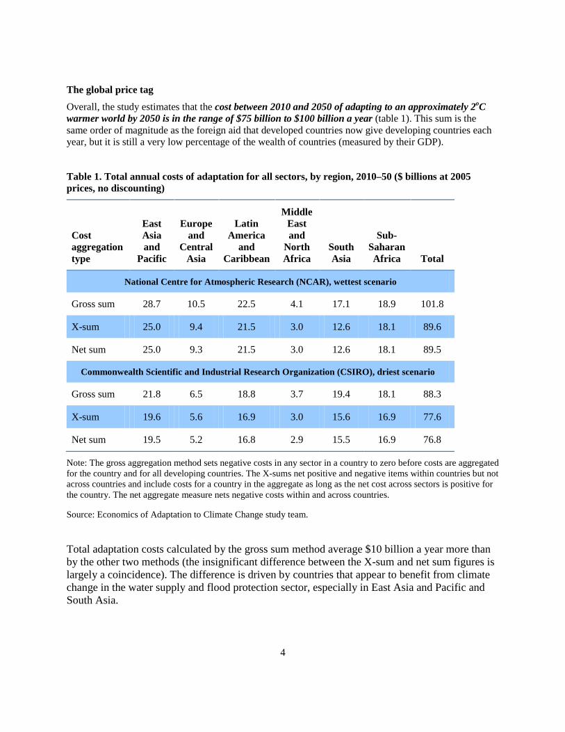
Water supply. Climate change has already affected the hydrological cycle, a process that is expected to intensify over the course of the 21st century. In some parts of the world, water availability has increased and will continue to increase, but in other parts, it has decreased and will continue to do so. Moreover, the frequency and magnitude of floods are expected to rise, because of projected increases in the intensity of rainfall. Accounting for the climate impacts, the study shows that water supply and flood management ranks as one of the top three adaptation costs in both the wetter and drier scenarios, with Sub-Saharan Africa footing by far the highest costs. Latin America and the Caribbean also sustain high costs under both models, and South Asia sustains high costs under CSIRO.

Agriculture. Climate change affects agriculture by altering yields and changing areas where crops can be grown. The EACC study shows that changes in temperature and precipitation from both climate scenarios will significantly hurt crop yields and production—with irrigated and rainfed wheat and irrigated rice the hardest hit. South Asia shoulders the biggest declines in production but developing countries fare worse for almost all crops compared to developed countries. Moreover, the changes in trade flow patterns are dramatic. Under the NCAR, developed country exports increase by 28 percent while under the CSIRO they increase by 75 percent compared with 2000 levels. South Asia becomes a much larger importer of food under both scenarios, and East Asia and Pacific becomes a net food exporter under the NCAR. In addition, the decline in calorie availability brought about by climate change raises the number of malnourished children.

Human health. The key human health impacts of climate change include increases in the incidence of vector-borne disease (malaria), water-borne diseases (diarrhea), heat- and cold-related deaths, injuries and deaths from flooding, and the prevalence of malnutrition. The EACC study, which focuses on malaria and diarrhea, finds adaptation costs falling in absolute terms over time to less than half the 2010 estimates of adaptation costs by 2050. Why do costs decline in the face of higher risks? The answer lies in the benefits expected from economic growth and development. While the declines are consistent across regions, the rate of decline in South Asia and East Asia and Pacific is more rapid than in Sub-Saharan Africa. As a result, by 2050 more than 80 percent of the health sector adaption costs will be shouldered by Sub-Saharan Africa.

Extreme weather events. In the absence of reliable data on emergency management costs, the EACC study tries to shed light on the role of socioeconomic development in increasing climate resilience. It asks: As climate change increases potential vulnerability to extreme weather events, how many additional young women would have to be educated to neutralize this increased vulnerability? And how much would it cost? The findings show that by 2050, neutralizing the impact of extreme weather events requires educating an additional 18 million to 23 million young women at a cost of $12 billion to $15 billion a year. For the period 2000–50 as a whole, the tab reaches about $300 billion in new outlays. This means that in the developing world, neutralizing the impact of worsening weather over the coming decades will require educating a large new cohort of young women at a cost that will steadily escalate to several billion dollars a year. However, it will be enormously worthwhile on other margins to invest in education for millions of young women who might otherwise be denied its many benefits.

10

Putting the findings in context

How does this study compare with earlier studies? The EACC estimates are in the upper end of estimates provided by the UNFCCC (2007), the study closest in approach to the EACC (table 2), although not as high as suggested by a recent critique of the UNFCCC study by Parry and others (2009). Why are the EACC estimates so much higher than those of the UNFCCC? To begin with, even though a comparison of the studies is limited by a number of methodological differences (in particular, the use of a consistent set of climate models to link impacts to adaptation costs and an explicit separation of costs of development from those of adaptation in the EACC study), the major difference between them is the sixfold increase in the cost of coastal zone management and defense under the EACC study. This difference reflects several improvements to the earlier UNFCCC estimates under the EACC study: better unit cost estimates, including maintenance costs, and the inclusion of costs of port upgrading and risks from both sea-level rise and storm surges. Table 2. Comparison of adaptation cost estimates by the United Nations Framework Convention on Climate Change and the Economics of Adaptation to Climate Change

Sector

United Nations Framework

Convention on Climate Change

(2007)

Economics of Adaptation to Climate Change study

National Centre for Atmospheric

Research (NCAR), wettest scenario

Commonwealth Scientific and

Industrial Research Climate (CSIRO),

driest scenario

Infrastructure 2-41 29.5 13.5

Coastal zones 5 30.1 29.6

Water supply and flood protection

9 13.7 19.2

Agriculture, forestry, fisheries 7 7.6 7.3

Human health 5 2 1.6

Extreme weather events — 6.7 6.5

Total 28-67 89.6 77.7

Source: UNFCCC (2007) and Economics of Adaptation to Climate Change study team. Another reason for the higher estimates is the higher costs of adaptation for water supply and flood protection under the EACC study, particularly for the drier climate scenario, CSIRO. This difference is explained in part by the inclusion of riverine flood protection costs under the EACC study. Also pushing up the EACC study estimate is the study’s comprehensive sector coverage, especially inclusion of the cost of adaptation to extreme weather events.

11

The infrastructure costs of adaptation in the EACC study fall in the middle of the UNFCCC range because of two contrary forces. Pushing up the EACC estimate is the more detailed coverage of infrastructure. Previous studies estimated adaptation costs as the costs of climate-proofing new investment flows and did not differentiate risks or costs by type of infrastructure. The EACC study extended this work to estimate costs by types of infrastructure services—energy, transport, water and sanitation, communications, and urban and social infrastructure. Pushing down the EACC study estimate are measurements of adaptation against a consistently projected development baseline and use of a smaller multiplier on baseline investments than in the previous literature, based on a detailed analysis of climate proofing, including adjustments to design standards and maintenance costs. The one sector where the EACC study estimates are actually lower than the UNFCCC study is human health. The reason for this divergence is in part because of the inclusion of the development baseline, which reduces the number of additional cases of malaria, and thereby adaptation costs, by some 50 percent by 2030 under the EACC study.

The bottom line is that calculating the global cost of adaptation remains a complex problem, requiring projections of economic growth, structural change, climate change, human behavior, and government investments 40 years in the future. The EACC study has tried to establish a new benchmark for research of this nature, as it adopted a consistent approach across countries and sectors and over time. But in the process, it had to make important assumptions and simplifications, to some degree biasing the estimates.

• Adaptation costs are calculated as though decisionmakers knew with certainty what the future climate will be, when in reality the current climate knowledge does not permit even probabilistic statements about country-level climate outcomes. In a world where decisionmakers hedge against a range of outcomes, the costs of adaptation could be potentially higher.

• Of the many global climate projections available for the baseline, only the set reporting maximum and minimum temperatures—and within that set, only the two yielding the wettest and the driest outcomes—were used. In addition, only one growth path was applied. A limited sensitivity analysis finds that a small number of countries face enormous variability in the costs of adapting to climate change given the uncertainty about the extent and nature of climate change. Moreover, the costs of managing these risks could be substantially higher.

• Climate science tells us that the impacts will increase over time and that major effects such as melting of ice sheets will occur further into the future. Even so, the study opted for projecting what is known today with greater certainty rather than making even less reliable longer-term estimates. Thus the investment horizon of this study is 2050 only. A longer time horizon would increase total costs of adaptation.

12

• The study looks only at additional public sector (budgetary) costs imposed by climate change, not the costs incurred by individuals and private agents. Similarly, the study generally opted for hard adaptation measures that require an engineering response rather than an institutional or behavioral response. Soft adaptation measures often can be more effective and can avoid the need for more expensive physical investment. But as a first-cut global study, it was not possible to know whether effective institutions and community-level collective action, which are preconditions for the implementation of soft actions, exist in a given setting. While incorporating private adaptation would increase cost estimates, including soft measures could potentially decrease them.

• Other limitations include not being able to incorporate innovation and technical change; leaving out local-level impacts, particularly the incidence on more vulnerable groups and the distributional consequences of adaptation; not examining migration; and only partially accounting for adaptation costs related to ecosystem services because of gaps in scientific understanding of the impact of climate change on ecosystems. Relaxing the first of these limitations could lead to significant reductions in adaptation costs, while a more comprehensive assessment of ecosystem services would lead to an increase.

Lessons and recommendations

Four lessons stand out from the study.

First, adaptation to a 2oC warmer world will be costly. The study puts the cost of adapting between 2010 and 2050 to an approximately 2oC warmer world by 2050 at $75 billion to $100 billion a year. The estimate is in the upper range of existing estimates, which vary from $4 billion to $109 billion. Although the estimate involves considerable uncertainty (especially on the science side), it gives policymakers—for the first time—a carefully calculated number to work with. The value added of the study lies in the consistent methodology used to estimate the cost of adaptation—in particular, the way the study operationalizes the concept of adaptation.

Second, the world cannot afford to neglect mitigation. Adapting to an even warmer world than the 2oC assumed for the study—on the order of 4oC above pre-industrial levels by the end of the century—would be much more costly. Adaptation minimizes the impacts of climate change, but it does not tackle the causes. If we are to avoid living in a world that must cope with the extinction of half of its species, the inundation of 30 percent of coastal wetlands, and a large increase in malnutrition and diarrheal and cardio-respiratory diseases, countries must take steps immediately to sharply reduce greenhouse gas emissions.

Third, development is imperative, but it must take a new form. Development is the most powerful form of adaptation. It makes economies less reliant on climate-sensitive sectors, such as agriculture. It boosts the capacity of households to adapt by increasing levels of incomes, health, and education. It enhances the ability of governments to assist by improving the institutional infrastructure. And it dramatically reduces the number of people killed by floods and affected by floods and droughts. But adaptation requires that we go about development differently: breeding crops that are drought and flood tolerant, climate-proofing

13

infrastructure, reducing overcapacity in the fisheries industry, and accounting for the uncertainty in future climate projections in development planning.

Countries may have to shift patterns of development or manage resources in ways that take account of the potential impacts of climate change. Often, the reluctance to change reflects the political and economic costs of changing policies and (quasi-) property rights that have underpinned decades or even centuries of development. Countries experiencing rapid economic growth have an opportunity to reduce the costs associated with the legacy of past development by ensuring that future development takes account of prospective changes in climate conditions. The clearest, and probably most rewarding, opportunities to reduce adaptation costs lie in the water sector, with coastal and flood protection. But other sectors also stand to benefit.

Fourth, uncertainties are large, so robust and flexible policies and more research are needed. The imprecision of models projecting the future climate is the major source of uncertainty and risk for decision makers. Thus, it is crucial to undertake research, collect data, and disseminate information so that if climate change turns out to have worse impacts than anticipated in 20 or 30 years, countries can respond more quickly and effectively. In the meantime, countries should pursue low-cost policies and investments on the basis of the best or median forecast of climate change at the country level. At the same time, countries should avoid making investments that will be highly vulnerable to adverse climate change outcomes. For durable climate-sensitive investments, strategies should maximize the flexibility to incorporate new climate knowledge as it emerges. Hedging against varying climate outcomes, for example by preparing for both drier and wetter conditions for agriculture, would raise the cost of adapting well beyond what has been estimated here.

14

Section 1. B ackgr ound and M otivation

All countries, developing and developed, need to adapt to climate change. Even if global emissions of greenhouse gases are drastically reduced and concentrations are stabilized at 450 parts per million (ppm) of equivalent carbon dioxide (CO2e), the annual global mean average temperature is expected to be 2oC above pre-industrial levels by the middle of the century.1

With a 2oC rise will come a higher incidence of intense rainfall events and a greater frequency and intensity of droughts, floods, heat waves, and other extreme weather events. Households, communities, and planners will need to take measures that “reduce the vulnerability of natural and human systems against actual and expected climate change effects” (IPCC 2007, p. 3). Development will require such adaptation, and development progress may even be reversed as the increased incidence of extreme weather events and rising sea levels results in higher mortality and loss of assets, drawing resources from development; as greater incidence of infectious and diarrheal diseases reverses development gains in health standards; and as temperature and precipitation changes reduce agricultural productivity and the payoffs from agricultural investments.

While countries need to adapt to manage the unavoidable, decisive mitigation is required to avoid the unmanageable. Unless the world begins immediately to substantially reduce greenhouse gas emissions, annual global mean average temperature will rise by some 2.5–7oC over pre-industrial levels by the end of the century. Temperature increases of more than 2oC will substantially increase the likelihood of irreversible and potentially catastrophic impacts such as the extinction of half of all species, inundation of 30 percent of coastal wetlands, and massive increases in malnutrition and diarrheal and cardio-respiratory diseases (World Bank 2010). Even with government interventions, societies and ecosystems will not be able to adapt to impacts of this magnitude. Mitigation, to avoid a further rise in greenhouse gas emissions, is the only way to deal with climate change that is not already inevitable.2

Adaptation will be costly, but there is little information about just how costly. Under the Bali Action Plan adopted at the 2007 United Nations Climate Change Conference, developed countries agreed to allocate “adequate, predictable, and sustainable financial resources and [to provide] new and additional resources, including official and concessional funding for developing country parties” (UNFCCC 2008) to help them adapt to climate change. The plan views international cooperation as essential for building capacity to integrate adaptation measures into sectoral and national development plans. Yet studies on the costs of adaptation (discussed in more detail later in the report) offer a wide range of estimates, from $4 billion to $109 billion a year. A recent critique of existing estimates suggests that these may be substantial underestimates (Parry and others 2009). Similarly, National Adaptation Programmes of Action, developed by the Least Developed Countries under Article 4.9 of the United Nations Framework Convention on Climate Change (UNFCCC), identify and cost only urgent and immediate adaptation measures and do not incorporate the measures into long-term development plans.

1 With current greenhouse gas concentrations at about 400 parts per million, annual average global temperature is already 0.8oC above pre-industrial levels. 2 Mitigation is not discussed in this report, which focuses on adaptation.

15

This Economics of Adaptation to Climate Change (EACC) study is intended to fill this knowledge gap. Soon after the Bali Conference of Parties, a partnership of the governments of Bangladesh, Plurinational State of Bolivia, Ethiopia, Ghana, Mozambique, Samoa, and Vietnam and the World Bank initiated the EACC study to estimate the cost of adapting to climate change. The study, funded by the governments of the Netherlands, Switzerland, and the United Kingdom, also aims to help countries develop plans that incorporate measures necessary to adapt to climate change.

16

Section 2. Study Objectives and Str uctur e

The EACC study has two broad objectives: to develop a global estimate of adaptation costs for informing the international community’s efforts to help the developing countries most vulnerable to climate change meet adaptation costs, and to help decisionmakers in developing countries assess the risks posed by climate change and design strategies for adapting to climate change. That requires costing, prioritizing, sequencing, and integrating robust adaptation strategies into development plans and budgets. And it requires strategies to deal with high uncertainty, potentially high future damages, and competing needs for investments for social and economic development. Supporting developing country efforts to design adaptation strategies requires incorporating country-specific characteristics and sociocultural and economic conditions into analyses. Providing macro-level information to developed and developing countries to support international negotiations and to identify the overall costs of adaptation to climate change requires analysis at a more aggregate level. Reconciling the two needs involves a tradeoff between the specifics of individual countries and a global picture. The methodology developed for this study met both objectives by linking the country-level analysis with the analysis for estimating the global costs of adaptation. Initially, the intention was to use country case studies to develop unit least costs of adaptation and then to apply them to similar adaptation conditions in other developing countries. As the country level analysis got under way, however, it became clear that generalizing from the seven country cases (the seven partnering countries) would not work. A two-track approach—a global track to meet the first study objective and a case study track to meet the second—would yield a more robust estimate. For the global track, country-level data sets with global coverage are used to estimate adaptation costs for all developing countries by sector—infrastructure, coastal zones, water supply and flood protection, agriculture, fisheries and ecosystem services, human health, and forestry. The cost implications of changes in the frequency of extreme weather events are also considered. For most sectors, a consistent set of future climate and precipitation projections are used to establish the nature of climate change, and a consistent set of GDP and population projections are used to establish a baseline of how development would look in the absence of climate change. This information is used to establish economic and social impacts and the costs of adaptation (left side of figure 1). For the country track, the impacts of climate change and adaptation costs are being established only for the major economic sectors in each case study country (see right side of figure 1). To complement the global analysis, vulnerability assessments and participatory scenario development workshops are being used to highlight the impact of climate change on vulnerable groups and to identify appropriate adaptation strategies (see box 1). Macroeconomic analyses are being used to integrate the sectoral analyses and to identify cross-sector effects, such as relative price changes. Finally, in two country case studies (Bolivia and Samoa), an investment model is being developed to prioritize and sequence adaptation measures (see box 2).

17

Figure 1. Economics of Adaptation to Climate Change study structure: global and country tracks

Global track

Country track


The two tracks are intended to inform each other, to improve the overall quality of the analysis. This report presents the methodology and the results for the global track. The report for the case study track will be released early in 2010, by which time lessons from the country studies will be used to validate and improve the estimate of total adaptation costs, resulting in a final report of the global track in early 2010.

Though the current report has undergone intensive review, with an internal World Bank review of the concept note, methodology note, and draft report and reviews of draft sector chapters by an external and an internal expert, the current report is nonetheless considered a consultation draft. Revisions to account for comments received during the consultation process with a wide range of stakeholders will also be incorporated in the final report.

Box 1. Understanding what adaptation means for the most vulnerable social groups

The negative impacts of climate change will be experienced most intensely by the poorest people in developing countries. Just as development alone will not be enough to equip all countries or regions to adapt to climate change, neither do all individuals or households within a country or region enjoy the same levels of adaptive capacity (Mearns and Norton forthcoming). Drivers of physical, economic, and social vulnerability (socioeconomic status, dependence on natural resource based livelihood sources, and physical location, compounded by factors that shape social exclusion such as gender, ethnicity, and migrant status) act as multipliers of climate risk for poor households. Social variables further interact with institutional arrangements that are crucial in promoting adaptive capacity, including those that increase access to information, voice, and civic representation in setting priorities in climate policy and action (World Bank 2010).

Work is under way in six developing countries (Bangladesh, Plurinational State of Bolivia, Ethiopia, Ghana, Mozambique, and Vietnam) under the EACC study to understand what adaptation means for social groups that are most vulnerable to the effects of climate change and what external support they need to help them take adaptation measures. This social component of the study combines vulnerability

18

assessments in selected geographic hotspots with facilitated workshops applying participatory scenario development approaches. In the workshops, participants representing the interests of vulnerable groups identify preferred adaptation options and sequences of interventions based on local and national climate and economic projections. This approach complements the sectoral analyses of the costs of climate change adaptation in those countries. The findings on what forms of adaptation support various groups consider to be most effective—including “soft” adaptation options such as land use planning, greater public access to information, institutional capacity building, and integrated watershed management—have implications for the costs of adaptation. While this work is ongoing, some preliminary results from the country investigations in Bangladesh, Bolivia, Ethiopia, Ghana, and Mozambique are presented throughout this report to illustrate the range of adaptation options that are being suggested.

Box 2. Climate-resilient investment planning

A three-step methodology has been developed to help planners integrate climate risk and resilience into development policies and planning. The first is to identify and validate climate-resilient investment alternatives using a multicriteria decision analysis. This involves qualitative and quantitative impact assessments for each sector, consultation at the national level (government, policymakers, technical experts), and participatory workshops with community representatives and local authorities at the county level. The second step is to conduct a cost-benefit analysis for identified climate-resilient investment alternatives at a specific geographic unit. The final step is implementation of an investment planning model that allows the government to prioritize and sequence robust adaptation strategies into development plans and budgets.

19

Section 3. Oper ational Definition of A daptation C osts

One of the biggest challenges of the study has been to operationalize the definition of adaptation costs. The concept is intuitively understood as the costs incurred by societies to adapt to changes in climate. The Intergovernmental Panel on Climate Change (IPCC) defines adaptation costs as the costs of planning, preparing for, facilitating, and implementing adaptation measures, including transaction costs. But this definition is hard to operationalize. For one thing, “development as usual” needs to be conceptually separated from adaptation. That requires deciding whether the costs of development initiatives that enhance climate resilience ought to be counted as part of adaptation costs. It also requires deciding how to incorporate in those costs the adaptation deficit, defined as countries’ inability to deal with current and future climate variability. It requires defining how to deal with uncertainty about climate projections and impacts. And it requires specifying how potential benefits from climate change in some sectors and countries offset, if at all, adaptation costs in another sector or country.

L inks between adaptation and development The climate change literature examines several links between adaptation and development. Many studies argue that economic development is the best hope for adaptation to climate change: development enables an economy to diversify and become less reliant on sectors such as agriculture that are most likely to be vulnerable to the effects of climate change. Development also makes more resources available for abating risk. And often the same measures promote development and adaptation. For example, progress in eradicating malaria helps countries develop and also helps societies adapt to the rising incidence of malaria that may accompany climate change. Adaptation to climate change is also viewed as essential for development: unless agricultural societies adapt to changes in temperature and precipitation (through changes in cropping patterns, for example), development will be delayed. Finally, adaptation requires a new type of climate-smart development that makes countries more resilient to the effects of climate change. Urban development without attention to drainage, for example, will exacerbate the flooding caused by heavy rains. These links suggest that adaptation measures range from discrete adaptation (interventions for which “adaptation to climate change is the primary objective”; WRI 2007) to climate-smart development (interventions to achieve development objectives that also enhance climate resilience) to development not as usual (interventions that can exacerbate the impacts of climate change and that therefore should not be undertaken). Since the Bali Action Plan calls for “new and additional” resources to meet adaptation costs, this report defines adaptation costs as additional to the costs of development. Consequently, the costs of measures that would have been undertaken even in the absence of climate change are not included in adaptation costs, while the costs of doing more, doing different things, and doing things differently are included.

Defining the adaptation deficit Adaptation deficit has two meanings in the literature on climate change and development. One captures the notion that countries are underprepared for current climate conditions, much less for future climate change. Presumably, these shortfalls occur because people are underinformed about climate uncertainty and therefore do not rationally allocate resources to adapt to current climate events. The shortfall is not the result of low levels of development but of less than optimal allocations of limited resources resulting

20

in, say, insufficient urban drainage infrastructure. The cost of closing this shortfall and bringing countries up to an “acceptable” standard for dealing with current climate conditions given their level of development is one definition of the adaptation deficit (figure 2). The second, perhaps more common, use of the term captures the notion that poor countries have less capacity to adapt to change, whether induced by climate change or other factors, because of their lower stage of development. A country’s adaptive capacity is thus expected to increase with development. This meaning is perhaps better captured by the term development deficit.

Figure 2. A simplified interpretation of adaptation deficit

Source: Economics of Adaptation to Climate Change study team. The adaptation deficit is important in this study for establishing the development baseline from which to measure the independent, additional effects of climate change. For example, should the costs of climate-proofing infrastructure be measured relative to current provisions or to the levels of infrastructure countries would have had if they had no adaptation deficit? Because the adaptation deficit deals with current climate variability, the cost of closing the deficit is part of the baseline and not of the adaptation costs. Unfortunately, except in the most abstract modeling exercises, the costs of closing the adaptation deficit cannot be made operational (see box 3). This study therefore does not estimate the costs of closing the adaptation deficit and does not measure adaptation costs relative to a baseline under which the adaptation deficit has been closed. It is not obvious whether analyses that take a different approach and measure costs of adaptation relative to a baseline in which the adaptation deficit has been closed would estimate higher or lower adaptation costs. In infrastructure, for example, closing the adaptation deficit implies that a larger stock of infrastructure assets need be to climate-proofed, so closing the deficit in this sector could increase adaptation costs. In contrast, closing the adaptation deficit in agriculture might imply a lower percentage of rain-fed agriculture and therefore a lower impact of climate-change-induced droughts. Adaptation costs are likely to be reduced in the agricultural sector as a result. Analyses that include the costs of closing the adaptation deficit in the costs of adaptation are likely to estimate higher adaptation costs than those in this study.

Additional capacity needed to handle future climate change ADAPTATION COSTS

Capacity to address current climate variation

ADAPTATION DEFICIT

Appropriate capacity to deal with current climate variation

Appropriate capacity to deal with future climate change

21

Box 3. Difficulties in operationalizing the adaptation deficit

Determining an acceptable level of adaptation to current climate variability is challenging. Some observers consider the cost of closing the adaptation deficit as the cost of making all developing countries—whatever their level of development—as prepared for current climate events as developed countries are. Others argue that the amount countries spend should depend on conditions in the country. For example, a poor country may devote fewer resources (than a rich country) on preventing loss of lives from storm surges and more resources on fighting malaria if more lives can be saved for the same amount of resources. Because these hard choices are necessary in a resource-constrained world, differences in the amount of resources devoted to adapting to current climate variability cannot be used as a proxy for the adaptation deficit. Establishing the existence of an adaptation deficit requires first establishing that the benefit-cost ratio of expenditures in climate-sensitive areas exceed those of expenditures in all other sectors. Then estimating the size of the adaptation deficit requires estimating the degree of government underspending in climate-sensitive areas relative to all other areas of the economy. Deficits for all developing countries would then need to be estimate to estimate the “global” adaptation deficit—clearly not feasible.

E stablishing the development baseline Establishing the magnitude of the adaptation deficit is not relevant for this study. Establishing the development baseline is. This is done sector by sector and assumes that countries grow along a “reasonable” development path. In agriculture, it is done by imposing exogenous, reasonable growth conditions on current development achievements, such as exogenous productivity growth, area expansion, and investments in irrigation. In other sectors, such as infrastructure, the baseline is established by considering historical levels of infrastructure provision, such as paved road density and length of sewer pipes, in countries at different levels of development. Table 1 shows the definition of the development baseline adopted for each sector.

Table 1. Definition of development baseline, by sector

Sector Development Baseline Infrastructure Average sector performance by income groups Coastal zones Efficient protection of coastline Water supply and flood protection

Average municipal and industrial water demand by income groups; efficient protection against monthly flood with given return period

Agriculture Exogenous productivity growth, area expansion, investment in irrigation

Fisheries Maintenance of 2010 fish stocks Human health Health standard by income groups Forestry and ecosystem services

Not establisheda

Extreme weather events GDP-induced changes in mortality and numbers affected a. For reasons discussed in section 5, development baselines were not established for this sector. Source: Economics of Adaptation to Climate Change study team.

22

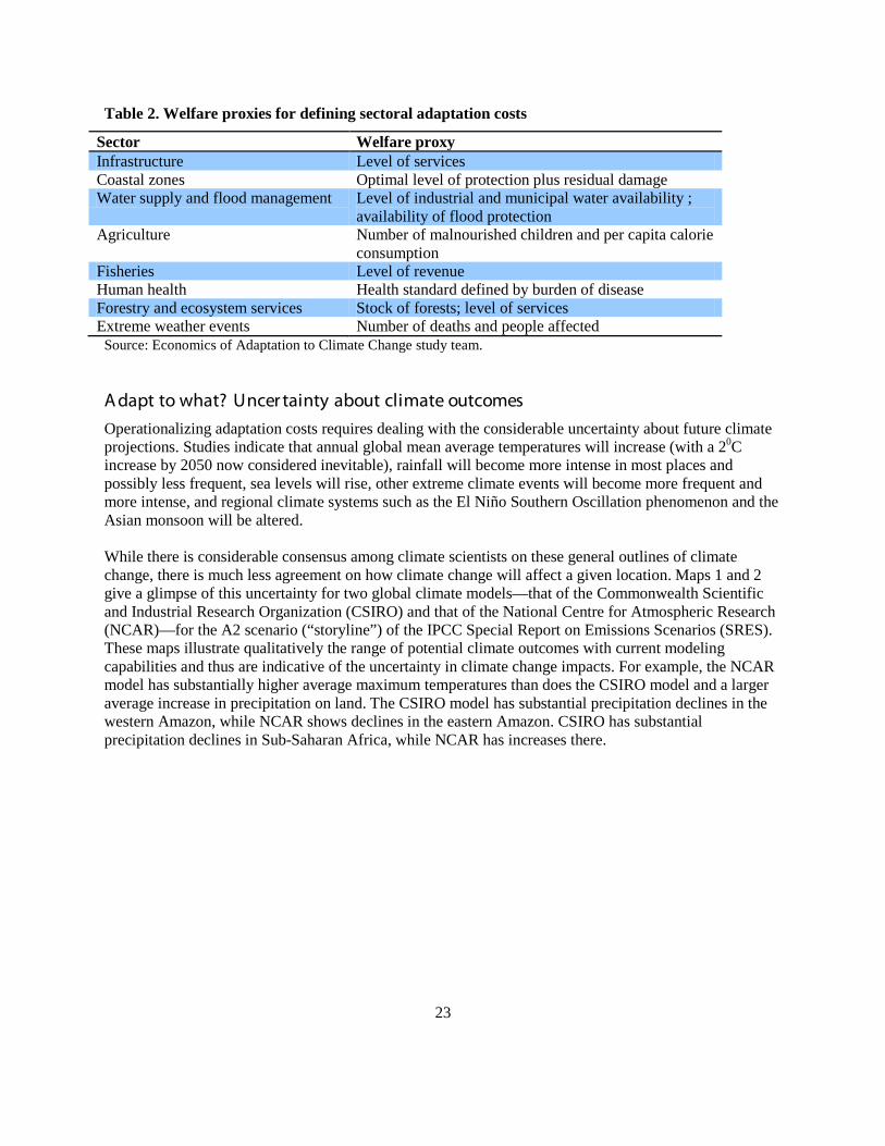
H ow much to adapt The next issue is how much to adapt. One possibility is to adapt completely, so that society is at least as well off as it was before climate change. At the other extreme, countries could choose to do nothing, experiencing the full impact of climate change. Or countries could invest in adaptation using the same criteria as for other development projects, investing until the marginal benefits of the adaptation measure exceed the costs, which could lead to either to an improvement or a deterioration in social welfare relative to a baseline without climate change. How much to adapt is consequently an economic problem—how to allocate resources to adapt to climate change while also meeting other needs. And herein lies the challenge. Poor urban workers who live in a fragile slum dwelling might find it difficult to decide whether to spend money to strengthen their hut to make it less vulnerable to more intense rainfall, or to buy school books or first-aid equipment for their family—or how to allocate between the two. Poor rural peasants might find it difficult to choose between meeting these basic education and health needs and some simple form of irrigation to compensate for increased temperatures and their impact on agricultural productivity. These examples suggest that desirable and feasible levels of adaptation depend on both available income and other resources. Corresponding to a chosen level of adaptation is an operational definition of adaptation costs. If the policy objective is to adapt fully, then the cost of adaptation can be defined as the minimum cost of adaptation initiatives needed to restore welfare to levels prevailing before climate change. Restoring welfare may be prohibitively costly, however, and policymakers may choose an efficient level of adaptation instead. Adaptation costs would then be defined as the cost of restoring pre-climate change welfare standards to levels at which marginal benefits exceed marginal costs. Because welfare would not be fully restored, there would be residual damage from climate change after allowing for adaptation. In this study, largely due to limitations of existing models, adaptation costs are generally defined as the costs of development initiatives needed to restore welfare to levels prevailing before climate change and not as optimal levels of adaptation plus residual damage (to the extent that residual damages are compensated, original welfare is restored). The one exception is coastal zones, where adaptation costs are defined as the cost of measures to establish the optimal level of protection plus residual damage. This study assumption is expected to bias the estimates upwards. Since costs are estimated by sector, sectoral proxies for welfare were identified (table 2). In agriculture, for example, welfare is defined by the number of malnourished children and per capita calorie consumption.

23

Table 2. Welfare proxies for defining sectoral adaptation costs

Sector Welfare proxy Infrastructure Level of services Coastal zones Optimal level of protection plus residual damage Water supply and flood management Level of industrial and municipal water availability ;

availability of flood protection Agriculture Number of malnourished children and per capita calorie

consumption Fisheries Level of revenue Human health Health standard defined by burden of disease Forestry and ecosystem services Stock of forests; level of services Extreme weather events Number of deaths and people affected


A dapt to what? Uncer tainty about climate outcomes Operationalizing adaptation costs requires dealing with the considerable uncertainty about future climate projections. Studies indicate that annual global mean average temperatures will increase (with a 20C increase by 2050 now considered inevitable), rainfall will become more intense in most places and possibly less frequent, sea levels will rise, other extreme climate events will become more frequent and more intense, and regional climate systems such as the El Niño Southern Oscillation phenomenon and the Asian monsoon will be altered. While there is considerable consensus among climate scientists on these general outlines of climate change, there is much less agreement on how climate change will affect a given location. Maps 1 and 2 give a glimpse of this uncertainty for two global climate models—that of the Commonwealth Scientific and Industrial Research Organization (CSIRO) and that of the National Centre for Atmospheric Research (NCAR)—for the A2 scenario (“storyline”) of the IPCC Special Report on Emissions Scenarios (SRES). These maps illustrate qualitatively the range of potential climate outcomes with current modeling capabilities and thus are indicative of the uncertainty in climate change impacts. For example, the NCAR model has substantially higher average maximum temperatures than does the CSIRO model and a larger average increase in precipitation on land. The CSIRO model has substantial precipitation declines in the western Amazon, while NCAR shows declines in the eastern Amazon. CSIRO has substantial precipitation declines in Sub-Saharan Africa, while NCAR has increases there.

24

Map 1. Projected change in average maximum temperature based on two climate models, 2000–50

Commonwealth Scientific and Industrial Research Organization (CSIRO), driest

scenario


Note: Projections are based on the A2 scenario of the IPCC Special Report on Emissions Scenarios (SRES). The Economics of Adaptation to Climate Change study team acknowledges the Program for Climate Model Diagnosis and Intercomparison and the World Climate Research Programme's (WCRP) Working Group on Coupled Modelling for their roles in making available the WCRP’s Coupled Model Intercomparison Project phase 3 (CMIP3) multimodel dataset. Support of this dataset is provided by the Office of Science, U.S. Department of Energy.

Source: Maps are based on data developed at the MIT Joint Program for the Science and Policy of Global Change using CMIP3 data (the WCRP’s CMIP3) multimodel dataset. Maps were produced by the International Food Policy Research Institute.

Map 2. Projected change in average annual precipitation based on two climate models, 2000–50


scenario


Note: Projections are based on the A2 scenario of the IPCC Special Report on Emissions Scenarios (SRES). The Economics of Adaptation to Climate Change study team acknowledges the Program for Climate Model Diagnosis and Intercomparison and the World Climate Research Programme's (WCRP) Working Group on Coupled Modelling for their roles in making available the WCRP’s Coupled Model Intercomparison Project phase 3 (CMIP3) multimodel dataset. Support of this dataset is provided by the Office of Science, U.S. Department of Energy.

25


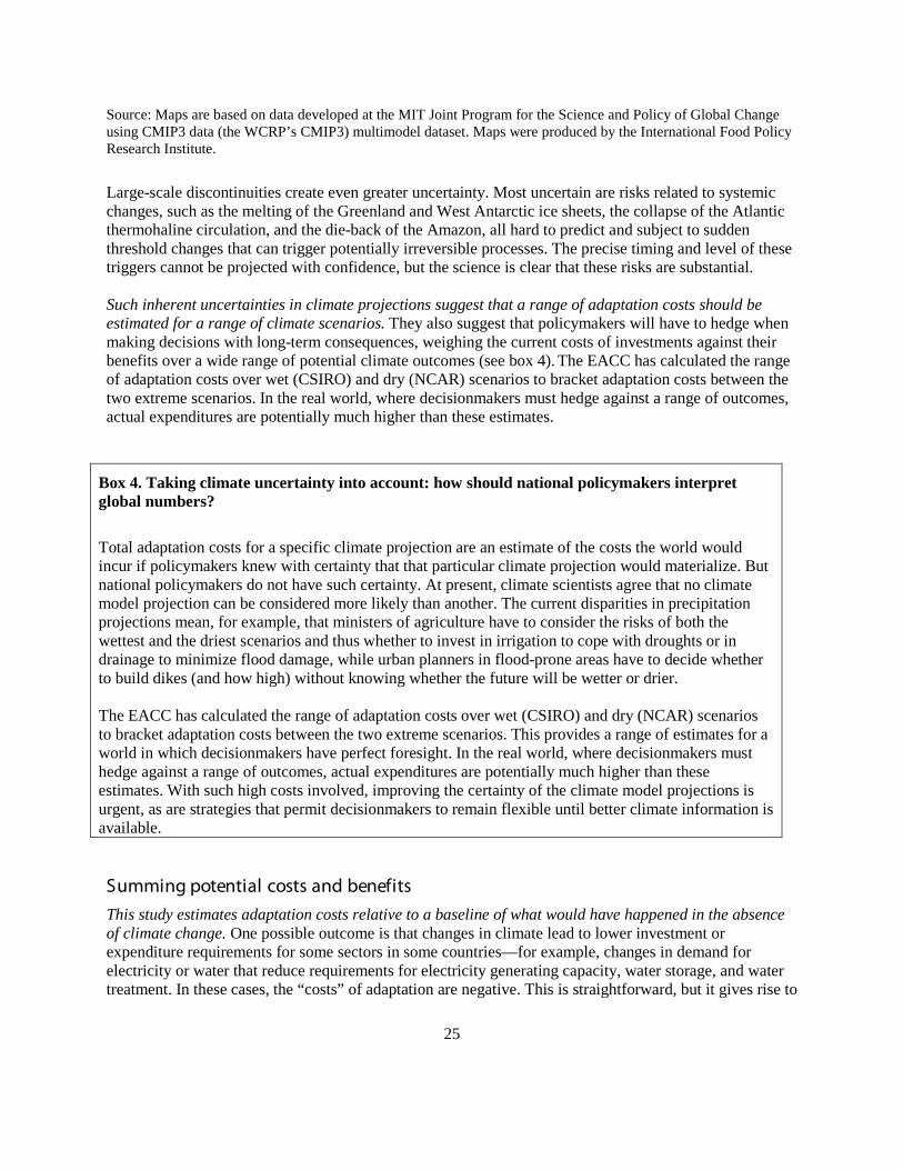
Large-scale discontinuities create even greater uncertainty. Most uncertain are risks related to systemic changes, such as the melting of the Greenland and West Antarctic ice sheets, the collapse of the Atlantic thermohaline circulation, and the die-back of the Amazon, all hard to predict and subject to sudden threshold changes that can trigger potentially irreversible processes. The precise timing and level of these triggers cannot be projected with confidence, but the science is clear that these risks are substantial. Such inherent uncertainties in climate projections suggest that a range of adaptation costs should be estimated for a range of climate scenarios. They also suggest that policymakers will have to hedge when making decisions with long-term consequences, weighing the current costs of investments against their benefits over a wide range of potential climate outcomes (see box 4). The EACC has calculated the range of adaptation costs over wet (CSIRO) and dry (NCAR) scenarios to bracket adaptation costs between the two extreme scenarios. In the real world, where decisionmakers must hedge against a range of outcomes, actual expenditures are potentially much higher than these estimates.

Box 4. Taking climate uncertainty into account: how should national policymakers interpret global numbers?

Total adaptation costs for a specific climate projection are an estimate of the costs the world would incur if policymakers knew with certainty that that particular climate projection would materialize. But national policymakers do not have such certainty. At present, climate scientists agree that no climate model projection can be considered more likely than another. The current disparities in precipitation projections mean, for example, that ministers of agriculture have to consider the risks of both the wettest and the driest scenarios and thus whether to invest in irrigation to cope with droughts or in drainage to minimize flood damage, while urban planners in flood-prone areas have to decide whether to build dikes (and how high) without knowing whether the future will be wetter or drier. The EACC has calculated the range of adaptation costs over wet (CSIRO) and dry (NCAR) scenarios to bracket adaptation costs between the two extreme scenarios. This provides a range of estimates for a world in which decisionmakers have perfect foresight. In the real world, where decisionmakers must hedge against a range of outcomes, actual expenditures are potentially much higher than these estimates. With such high costs involved, improving the certainty of the climate model projections is urgent, as are strategies that permit decisionmakers to remain flexible until better climate information is available.

Summing potential costs and benefits This study estimates adaptation costs relative to a baseline of what would have happened in the absence of climate change. One possible outcome is that changes in climate lead to lower investment or expenditure requirements for some sectors in some countries—for example, changes in demand for electricity or water that reduce requirements for electricity generating capacity, water storage, and water treatment. In these cases, the “costs” of adaptation are negative. This is straightforward, but it gives rise to

26

another question: how should positive and negative costs be summed across sectors or countries? It is easy to envisage that higher expenditures on coastal protection could be offset by lower expenditures on electricity generation in the same country, but it is unlikely that higher expenditures on electricity generation in country A can be offset by lower expenditures in the same sector in country B.3

How then to define aggregates that add up consistently across sectors and countries?

Box 5 illustrates three options for summing positive and negative costs when there are restrictions on offsetting negative and positive items: gross, net, and X-sums. Under the gross aggregation method, negative costs in any sector in a country are set to zero before costs are aggregated for the country and for all developing countries. Under X-sums positive and negative items are netted within countries but not across countries, and costs for a country are included in the aggregate as long as the net cost across sectors is positive for the country. In the net aggregate measure, negative costs are netted within and across countries. The net calculation is carried out by decade. Of 146 developing countries, 10 have negative net adaptation costs in at least one decade across all sectors with the CSIRO scenario and 5 with the NCAR scenario. Most of these countries are landlocked, buffering them from the substantial costs for coastal protection that constitute a large part of the adaptation costs for coastal countries. All three options are used in the study to estimate adaptation costs, though costs are mainly reported as X-sums in the interest of space.

3 A simple example helps to illustrate the situation. Suppose that Brazil has a positive cost in both agriculture and water, meaning that both sectors will be negatively affected by climate change (relative to the no-climate-change scenario), and suppose that India has a negative cost in agriculture and a positive cost in water, meaning that agriculture benefits but the water sector suffers from climate change. It may be reasonable to assume that in India the gains in agriculture can compensate to some extent for the losses in the water sector. But it is unlikely that Brazil will be compensated by India because Brazil incurs a cost and India a benefit in the agriculture sector.

27

Box 5. Calculating aggregate costs—gross, net, and X-sums

In summing positive and negative adaptation costs across countries, whether for a single sector or all sectors, three types of aggregate can be constructed (as illustrated by the hypothetical figures in the table). Summing positive and negative adaptation costs

Sector and type of aggregate

Country Sector aggregate

A B C Sector gross Sector net

Sector X-sum

Sector 1 2 2 2 6 6 — Sector 2 8 –4 –2 8 2 — Sector 3 2 6 –4 8 4 — Country gross 12 8 2 22 — — Country net 12 4 –4 — 12 — Country X-sum 12 4 0 — — 16

— is not applicable. Gross sum. The gross sum represents the aggregate costs incurred by countries with positive costs for a particular sector, ignoring all country and sector combinations resulting in negative costs. One difficulty with gross sums is that the results vary depending on how sectors are defined. This can be illustrated by recalculating the gross sums after combining sectors 1 and 2, giving an overall sectoral gross sum of 18 rather than 22, even though nothing else has changed (not shown in table). Net sum. The net sum treats positive and negative values symmetrically. It represents the pooled costs incurred by each country or each sector without restrictions on pooling across country borders. X-sum. X-sums take account of restrictions on pooling across countries, so all entries for a given country are set to zero if the net sum for the country is negative (see country C in the table). For the hypothetical data in the table, the overall gross sum is 22, and the overall net sums is 12. The difference between the two values is the absolute value of negative entries for sectors 2 and 3 in countries B and C. The overall X-sum, which must fall between the overall gross and net sums, is 16. The difference between the overall X-sum and the overall net sum is 4, equal to the loss of pooling because of the net negative cost for country C.

28

Section 4. M ethodology and V alue Added

Although the methodology used to estimate the impacts of climate change and the costs of adaptation is specific to each sector, the sectoral methodologies share several elements. Adaptation costs in most sectors were calculated for 2010–50 from a common trajectory of population and GDP growth used to establish the development baseline and a common set of global climate models used to simulate climate effects. For all sectors, adaptation costs include the costs of planned, public policy adaptation measures and exclude the costs of private adaptation. For agriculture, for example, the methodology allows for the effects of autonomous adjustments in the private sector, such as changes in production, consumption, and trade flows in response to world price changes, but does not include the costs of those adjustments in adaptation costs. These common methodological elements, along with wide and in-depth sectoral coverage and a consistent definition of adaptation costs, allow the study to substantially improve on earlier estimates (box 6).

Box 6. Previous estimates of global adaptation costs

World Bank (2006). The first estimate of costs of adaptation to climate change for developing countries was produced by the World Bank in 2006. Its report defined adaptation costs as the cost of climate-proofing three categories of investment flows: official development assistance and concessional finance, foreign direct investment, and gross domestic investment. The study defined the proportion of total investments in each category that was likely to be climate sensitive and then estimated the percentage increases in costs to climate-proof these investments. Adaptation cost estimates ranged from $9 billion to $41 billion a year. Stern (2007) and UNDP (2007). Using the same methodology as World Bank (2006) but different values for the proportion of climate-sensitive investments and the increases in costs for climate-proofing investments, the Stern Report (Stern 2007) estimated costs of adaptation of $4– $37 billion a year by 2050, somewhat lower than the World Bank estimate, while Human Development Report 2007/2008 (UNDP 2007) estimated costs of $5–67 billion a year by 2015, somewhat higher than the World Bank estimate. In addition to the cost of climate-proofing investments, Human Development Report 2007/2008 also estimated that by $40 billion a year would be needed by 2015 to strengthen social protection programs and scale up aid in other key areas and $2 billion a year to strengthen disaster response systems, boosting overall adaptation costs to $47–109 billion a year by 2015. Oxfam International (2007). In contrast to this these top-down approaches, Oxfam International (2007) used a bottom-up approach, estimating adaptation costs by assessing National Action Plans for Adaptation and the costs of adaptation projects initiated by nongovernment organizations. Assuming average warming of 2oC, the report estimated global adaptation costs of at least $50 billion a year: $7.5 billion a year to support adaptation efforts initiated by nongovernmental organizations,1 $8–33 billion a year to meet the costs of the most urgent adaptation measures being proposed under the National Action Plans for Adaptation, and $5–15 billion a year to address unknown and unexpected impacts. Though richer in the range of potential adaptation measures, this methodology uses a small and likely unrepresentative sample of projects and countries to generalize to all developing countries. UNFCCC (2007). Whereas previous efforts considered only the costs of planned adaptation, the United Nations Framework Convention on Climate Change study considered the costs of both planned and

29

private adaptation measures. Also, whereas previous studies had considered costs across all sectors, this report estimated the costs of adaptation by major sectors (agriculture, forestry, and fisheries; water supply; human health; coastal zones; and infrastructure), yielding total costs of $26–67 billion a year by 2030. A recent critique of the UNFCCC estimates (Parry and others 2009) suggests that these estimates may be too low because some sectors were excluded (ecosystems, energy, manufacturing, retailing, and tourism), included sectors were not fully accounted for, climate-proofing of infrastructure stocks ignored the need for additional stocks (financed through full funding of development) for handling current climate variability, and residual damages (impacts remaining after adaptation) were not accounted for. Project Catalyst (2009). The final estimate was produced in 2009 by the Climate Works Foundation’s Project Catalyst initiative. This study estimated that annual average adaptation funding requirements for developing countries lie between $15 billion and $30 billion for the period 2010–20 and between $30 billion and $90 billion by 2030. Softer measures, such as capacity building, planning, and research, are the focus of adaptation policy in the first decade, followed by more expensive structural investments in the second decade. Unlike previous estimates, the study accounts for potential co-benefits of adaptation actions and reduces the cost estimate to reflect these benefits.

C hoosing the timefr ame The choice of timeframe for the analysis of the costs of adapting to climate change will likely affect the overall cost estimates, with a longer timeframe producing higher costs than would a shorter one. The timeframe up to 2050 was selected largely because forecasting climate change and its impacts on an economy becomes even more uncertain beyond this period, and the complexity of the analysis favors getting more precise (or less imprecise) estimates in the near term rather than less precise estimates over a more extended timeline. Related to the issue of timeframe is the choice of the discount rate, which is related to the timing of investments. The timing of all investments in the sector models is determined by the outcomes of specific climate projections. Given the expected climate outcome within the useful life of an investment, each new investment must be designed to restore welfare (as defined in table 2) to levels that would have existed without climate change. Because of the complexity of modeling sectors at a global level, none of the sectoral models is capable of choosing the optimal timing of investments. This implies that the time-paths of investments is insensitive to changes in the discount rate and therefore all results are presented for a zero discount rate though costs have been expressed in 2005 constant prices. Obviously, discounting the time stream of investment costs would lower the net present value of total investment or adaptation costs, but it would not influence the choice of investments or the underlying investment costs. The inability to model policy tradeoffs across time is a clear limitation imposed by the global nature of this study. The selection of the discount rate and intertemporal choices will be explored in depth in some of the country case studies.

Using baseline G DP and population pr ojections to account for continuing development Most studies of adaptation to climate change hold developing countries at their current level of development when estimating adaptation costs even over the medium term. Yet most developing countries will become economically more advanced over the medium term, which will alter the economic

30

impact of climate change and affect the type and extent of adaptation needed. As already explained, the EACC study accounts for the impact of development on estimates of adaptation costs by establishing development baselines by sector (see table 1). These baselines establish a fictional growth path in the absence of climate change that determines sectoral performance indicators, such as stock of infrastructure assets, level of nutrition, and water supply availability. Climate change impacts and costs of adaptation are examined in relation to this baseline. Baselines are established across sectors using a consistent set of future population and GDP projections. The population trajectory is aligned with the United Nations Population Division middle-fertility projections for 2006. To ensure consistency with emissions projections, the GDP trajectory is based on the average of the GDP growth projections of the three major integrated assessment models of global emissions growth—Climate Framework for Uncertainty, Negotiation, and Distribution (FUND; Anthoff and Tol 2008); PAGE2002 (Hope 2006); and Regional Dynamic Integrated Model of Climate and the Economy (RICE99; Nordhaus 2001), and growth projections used by the International Energy Agency and the Energy Information Administration of the US Department of Energy to forecast energy demand. All these sources provide growth estimates at a regionally disaggregated level. The global average annual real GDP per capita growth rate constructed in this way is 2.1 percent, similar to global growth rates assumed in the United Nations Framework Convention on Climate Change (UNFCCC) A2 emissions scenario from the IPCC 4th Assessment Report (AR4), once considered an extreme scenario but no longer (IPCC 2007). The regionally downscaled GDP projections under different IPCC scenarios (available from the Center for International Earth Science Information Network, Columbia University) were not used because they are based on older data.

C hoosing climate scenar ios and global climate models Twenty-six global climate models provide climate projections based on the IPCC A2 Special Report on Emission Scenarios (SRES) (see box 7). In this study, the National Center for Atmospheric Research (NCAR) CCSM3 and Commonwealth Scientific and Industrial Research Organization (CISRO) Mk3.0 models were used to model climate change for the analysis of most sectors because they capture a full spread of model predictions to represent inherent uncertainty and they report specific climate variables (minimum and maximum temperature changes) needed for sector analyses. Though the model predictions do not diverge much for projected temperature increases by 2050 (both projecting increases of approximately 2oC above pre-industrial levels), they vary substantially for precipitation changes. Among the models reporting minimum and maximum temperature changes, the NCAR was the wettest and the CSIRO the driest scenario (globally, not necessarily the wettest and driest in every location) based on the climate moisture index. Climate projections for these two models were created at a 0.5 by 0.5 spatial degree scale and a monthly time scale by applying model predictions through 2050 to a historical climate baseline obtained from the University of East Anglia Climate Research Unit’s Global Climate Database time series 2.1. Analysis was limited to two specific scenarios rather than the mean multiple of the global climate models because the mean masks extreme values. A model average of near zero could be the result of models predicting near-zero change, but just as well the result of two opposing changes that differ in sign. Using a group of global climate models (multimodel ensembles), as opposed to one model, can somewhat correct for biases and errors. The question with an ensemble approach is how to capture the full range of results from model runs.

31

Box 7. Special Report on Emissions Scenarios of the Intergovernmental Panel on Climate Change Adaptation requires understanding the potential impacts of climate change on human, economic, and ecological systems. Yet attempts to estimate such impacts have to take on a cascade of uncertainty. Uncertainty starts with the selection of an appropriate underlying emission scenario that is determined by economic and population growth and by energy use choices. Will the world grow rapidly or slowly? Will developing country populations soon adopt the consumption habits of high-income countries? And what kind of energy future are we to look forward to? To account for these questions, the Intergovernmental Panel on Climate Change (IPCC) has developed six socioeconomic scenarios that characterize possible trajectories of emissions. A scenario is a coherent, internally consistent, plausible description of a possible future state of the world. It is not a forecast; rather, each scenario is one alternative image of how the future can unfold, given a specific set of assumptions described in a set of four narrative storylines for the climate scenarios: A1 (focus on economic growth and globalization), A2 (regional focus), B1 (environmental focused), and B2 (regional focus). According to the IPCC, all families of scenarios from each storyline are equally valid, with no assigned probabilities of occurrence. The choice of climate and related nonclimate scenarios is important because it can determine the outcome of a climate impact assessment. According to the IPCC, however, all scenarios have more or less the same projected temperature increase up to 2050 (a timeframe arguably more relevant for adaptation), even though there are large uncertainties regarding carbon dioxide emissions within each scenario. Therefore, the selection of scenarios for this study depends largely on the availability of global climate model data as well as some range of most “likely” future scenarios for the location of interest.

Selecting adaptation measur es Adaptation measures can be classified by the types of economic agent initiating the measure—public or private. The literature distinguishes between autonomous or spontaneous adaptation (adaptation by households and communities acting on their own without public interventions but within an existing public policy framework) and planned adaptation (adaptation that results from a deliberate public policy decision). This study focuses on planned adaptation. This focus is not to imply that autonomous adaptation is costless. But since the objective is to help governments plan for risks, it is important to have an idea of what problems private markets will solve on their own, how public policies and investments can complement markets, and what measures are needed to protect public assets and vulnerable people. For that, assessment of planned adaptation is needed.

In all sectors except extreme weather events, “hard” options involving engineering solutions are favored over “soft” options based on policy changes and social capital mobilization (table 3). For adaptation to extreme weather events, the emphasis is on investment in human resources, particularly those of women. The decision to focus on hard options for the global cost assessment was motivated largely by fact that these are easier to cost. Though hard adaptation options are feasible in nearly all settings, while soft options depend on social and institutional capital, the focus on hard options is not to suggest that they are always preferable. As discussed in box 8, adaptation measures being identified in the companion case studies through participatory scenario workshops span both hard and soft measures. Since hard options are typically more expensive than soft ones, this study assumption is likely to give the estimates an upward bias.

32

Box 8. Adaptation measures identified in participatory workshops

Participants in the participatory scenario development workshop identified several cross-cutting climate change impacts in the infrastructure, natural resource management and agriculture, health and education, land tenure, governance and service delivery, and migration support sectors. Participatory scenario development methods were particularly good at eliciting information on intersectoral linkages among climate impacts and investments and the need for complementary investments. For example, female farmers and others in a local workshop in Kalu, Ethiopia, noted the multiple effects of climate variability on livelihood outcomes in the midland region. They noted that drought and water scarcity led to livestock disease, human health impacts, and reduced household farm productivity and income, resulting in the withdrawal of children from school, distress migration, and more detahs. Calls for adaptation support included investments in watershed management, drought-resistant crop varieties, nonfarm diversification, and capacity building. Local workshop participants in Xai-Xai, Mozambique, highlighted the different income groups within broad sectoral categories (such as commercial producers and nontimber forest collectors within agroforestry) and noted their varied preferences for adaptation investments (see table). In addition, participants in both workshops identified not only vulnerable populations but also dynamic processes of migration, urbanization, and market development that were leaving some households more vulnerable than others.

Livelihood groups identified in southern Mozambique participatory scenario development workshop

Sector Income tiers Key climate impacts Select adaptation options

sought

Fishing • Commercial fishers

• Artisanal fishers

• Sea level rise, abandonment of fishing

• Increased salinity in estuaries, reduced fluvial fisheries

• Introduction of new fish species

• Coastal zone pollution reduction measures

Agroforestry

• Harvesters (including

commercial harvesters)

• Charcoal producers and fuelwood collectors

• Construction pole gatherers

• Nontimber forestry product and food gatherers

• Cyclones, loss of coastal vegetation, ecosystem change

• Floods destroying forest access routes

• Drought, increased physical vulnerability and species change

• Reforestation and dune protection

• Improved road construction planning

• Community involvement and education

Trade and commerce

• Informal and formal sector trading

• Cyclones destroying infrastructure and

• Climate-proof infrastructure; improved early warning

33

• Differential access to market (seasonal traders, retail traders, wholesale)

displacing people

• Sea level rise, coastal erosion and reduced land for development

systems

• Improved erosion control through public works

Agriculture and ranching

• Large, medium, and subsistence farmers (both rainfed highland farmers and lowland/ floodplain farmers with irrigation)

• Floods and droughts, loss of production, increased livestock disease and death

• Cyclones, loss of lives, crops, infrastructure

• Salinity intrusion

• Barns for animals

• Improved early warning systems

• Better siting of farms

• Dam, floodgate construction

Source: Xai-Xai, Mozambique, participatory scenario development workshop report.

In all sectors except extreme weather events, “hard” options involving engineering solutions are favored over “soft” options based on policy changes and social capital mobilization (table 3). For adaptation to extreme weather events, the emphasis is on investment in human resources, particularly those of women. The decision to focus on hard options for the global cost assessment was largely motivated by fact that these are easier to cost. Though hard adaptation options are feasible in nearly all settings, while soft options depend on social and institutional capital, the focus on hard options is not to suggest that they are always preferable. As discussed in box 8 adaptation measures being identified in the companion case studies through participatory scenario workshops span both hard and soft measures. Since hard options are typically more expensive than soft ones, this study assumption is likely to give the estimates an upward bias.

Table 3. Types of adaptation measures considered, by sector

Sector Adaptation measure Infrastructure Design standards, climate-proofing maintenance Coastal zones River and sea dikes, beach nourishment, port upgrades Water supply and flood protection

Reservoir storage, recycling, rainwater harvesting, desalination; flood protection dikes and polders

Agriculture Agricultural research, rural roads, irrigation infrastructure expansion and efficiency improvements

Fisheries Fisheries buybacks, individual transferable quotas, fish farming, livelihood diversification measures, marine protected areas

Human health Prevention and treatment of disease Extreme weather events Investment in human resources


34

Under standing the limitations of this study Calculating the cost of adaptation for developing countries requires simplifying a complex problem involving multiple countries, institutions, decisionmakers, and projections of government investments into a world 40 years in the future. This requires constructing projections of economic growth, structural change, climate change, and human behavior over a long time horizon and for numerous sectors. Subject to these constraints, the study has adopted a consistent approach across countries and sectors and over time, establishing a new benchmark for research of this kind.

To do so, however, several important assumptions and simplifications had to be made. The features and limitations of the analysis for each sector are discussed in the sector analyses in section 5. This section looks at five important limitations of the overall study methodology that arise from the need to simplify the problem sufficiently to derive adaptation costs for all developing countries: characterization of government decisionmaking environment, limited range of climate and growth outcomes, limited scope in time and economic breadth, simplified characterization of human behavior, and top-down versus bottom up analysis.

Stylized char acter ization of gover nment decision-making envir onment

The characterization of government decisionmaking is the most problematic element of the study. As have all other attempts to estimate the total costs of adaptation, this study calculates adaptation costs as if decisionmakers knew with certainty what the future climate will be. In truth, current climate knowledge does not permit even probabilistic statements about country-level climate outcomes and therefore provides virtually no help in informing country-level decisionmakers’ investment decisions.4

In fact, with current climate knowledge, country-level decisionmakers face a different problem—how to maximize the flexibility of investment programs to take advantage of new climate knowledge as it becomes available. While this decision problem can be explored at the country level, it is intractable in a global study. Without the assumption of perfect foresight, it would be impossible to calculate adaptation cost for developing countries in all but the most highly stylized and aggregated models. If such an analysis were possible, though, costs of adaptation to climate change would likely be higher than those in this study.

For most durable investment decisions, decisionmakers know with certainty only that climate in the future will differ from climate today. The adaptation costs calculated in this study and in all other global studies are based on the fiction that decisionmakers know what future climate will be and act to prevent its damages.

L imited r ange of climate and gr owth outcomes

Even with this strongly stylized characterization of the decision problem, overall model complexity permits systematic exploration of only a small range of potential outcomes. The two major drivers of adaptation costs are climate outcome and economic growth. Of the 26 climate projections available for the A2 SRES, a complete assessment of adaptation costs was possible only with 2. Exploration of

4 Although some researchers have, as a practical expedient, constructed triangular probability densities to represent the range of global climate model outcomes, most climate scientist would object to this use of their data.

35

alternative growth paths was even more restricted, with only one future applied across all sectors.5

L imited scope in economic br eadth and time

Sensitivity analysis was performed in various sectors, however (as described later). For climate outcomes, sensitivity analysis suggests that one or two global climate models predict adaptation costs in several South Asian countries that are orders of magnitude greater than those of the other climate models. For growth, sensitivity analysis indicates that the results are much less sensitive than for climate outcomes, as would be expected. While more growth increases the assets at risk, it raises incomes and reduces vulnerability.

To make calculations tractable, the study had to limit both the breadth of economic analysis and the length of the time horizon. For the economic analysis, this means that the study has estimated only the additional public sector (budgetary) costs imposed by climate change, not overall economic damages. These additional costs for the provision of public goods must not be confused with overall economic damages and cannot be usefully compared with mitigation costs. The investment horizon of this study is to 2050 only. Climate science tells us that adaptation costs and damages will increase over time, and that major effects such as melting of major ice sheets are more likely to occur well beyond this horizon.

Simplified char acter ization of human behavior

H ar d adaptation ver sus soft adaptation. Hardest of all to project is human behavior, especially developments in institutions and the political economy. Many adaptive measures are best implemented through effective collective action at the community level. However, the circumstances that elicit effective collective action are complex (Ostrom 1990). “Soft” adaptation measures, such as early warning systems, community preparedness programs, watershed management, urban and rural zoning, and water pricing, generally rely on effective institutions supported by collective action. Because it is easier to cost hard measure and because it is impossible to know, in a global study, whether such preconditions exist in a given setting, this study has generally opted for hard adaptation measures that require an engineering response.6

M igr ation behavior . Decisions to migrate are also strongly mediated by community processes and social capital. Because social processes that create poverty and marginality are more important determinants of likely migration outcomes than are environmental changes themselves, in theory it should be possible to reduce the likelihood of migration arising from climate change. However, in the absence of vastly improved political and economic structures that can reduce poverty, environmental change will continue to be an important proximate factor in migration decisions (box 9). The estimates in this study are based on demographic projections by the United Nations Population Division that do not take climate change into account. Population movements across countries may impose heavy infrastructure costs in areas

Not a recommendation, this is rather a simplifying assumption to make the study tractable. To the extent that local institutions exist that can employ more effective and less expensive soft adaptation measures, this assumption imparts an upward bias to the global cost.

5 However, the growth path used in this study represents a consensus growth path among climate modelers and is chosen to be consistent with the emissions level underlying the A2 SRES. 6 An exception is the inclusion in the agriculture sector assessment of a number of soft measures such as water harvesting in the adaptation measure “irrigation reform”.

36

receiving substantial numbers of migrants. This is, however, more likely to become a serious issue in the second half of the century.

Box 9. Migration and climate change—Ghana’s experience

Climate change impacts are expected to induce large new migration flows. The number of environmental migrants (people moving in response to environmental degradation, extreme events, or related economic conditions; see Warner and others 2009) is projected to rise in coming decades, with the vast majority seeking residence in large cities. Migration was a recurring theme in the EACC participatory scenario development workshops, as well as in field-level investigations. This box highlights some key findings from Ghana.

Drought in the northern savannah region of Ghana has long triggered migration to the country’s coastal cities. Rural-urban migration creates vulnerabilities at a number of levels. New migrants live in informal housing and often in peri-urban areas without services. They also typically lack social ties and access to information in their new locations. Recent migrants to Accra reside in unplanned developments in highly risky sites including flood-prone and malarial marshlands. Migrants are disproportionately young men, leaving women, children, and the elderly to tend to agricultural lands and putting household farm production and food security at risk because of lack of household labor.

Rural-rural migration also leads to problems, especially in land access and ownership for production. Resource rights are tenuous for recent migrants—at least 80 percent of land in Ghana is administered through customary law institutions including local chiefdoms that can be exclusionary. Focus group participants in Dzatakpo, Ghana, stated that the local chief has given only land use rights to immigrants, rather than full land rights. Immigrants in Buoyem, Ghana, were reluctant to plant long-gestation (and higher value) crops because of insecure access to land. Sharecropping and use-right rules in the Western Region of Ghana also impede sustainable land management. Because failure to clear a piece of forested land for cultivation within two years of acquisition results in forfeiture, the rule leads to destruction of forest resources. Despite rising numbers of migrants to the Western Region, this customary practice has not changed, highlighting the slow pace of adaptation of some local institutions to changing circumstances.

Key policy responses to environmental migration include social protection support to migrants, such as easing place-based residence requirements for accessing social services; investing in sending regions so as to reduce the flow of migrants, as Ghana is doing with its northern development strategy; and considering rights-based resettlement for populations directly displaced by climate impacts, such as sea-level rise.

T he efficiency of adaptation. Economic models normally assume fully rational behavior—producers maximize profits, consumers maximize welfare, governments provide public goods using cost-benefit criteria to choose the most efficient projects, and projects are implemented optimally through time to maximizes the net present value of the government’s future investment stream. None of the sector models used in this study is capable of intertemporal optimization. Calculations in each sector ensure that service levels are maintained despite climate change, but no effort was made to identify whether the resources invested in one sector to counter the effects of climate change would have yielded a higher benefit-cost ratio in another sector (except in the sea-level rise component) or whether cash transfers would maintain welfare at less cost. As a result, the adaptation costs calculated in this study are almost certainly

37

inefficient, even within the framework of the study. This simplification imparts an upward bias to the adaptation costs.

I nnovation and technical change. Most parts of the study do not allow for the unknowable effects of innovation and technical change on adaptation costs. In effect, these costs are based on what is known today rather than what might be possible in 20–40 years. Sustained growth in per capita GDP for the world economy rests on technical change, which is likely to reduce the real costs of adaptation over time. This treatment of technological change also contributes to an upward bias in the calculated costs. The exception is agriculture. Growth in total factor productivity in agriculture, based on historical trends and expert opinion, is built into the model, and explicit investment in research is included in the costs.

T op-down or bottom-up analysis

In the final report of this study, this global approach will be supplemented by country case studies. But this report on the global track relies on a mixed top-down sectoral approach to country analysis because of the difficulty of generalizing from country studies when there is no clear basis for scaling up country results. It is “mixed” because, for countries that are too large and too heterogeneous to be treated as a single analytical unit, the basic analytical units include river basins and food production units. It would have been preferable to estimate the costs of adaptation for infrastructure at the subnational rather than national level in all countries with a population of, perhaps, 50–100 million or more. However, data availability and economic consistency are difficult to ensure at the subnational level.

38

Section 5. K ey R esults

This section presents the key results of the EACC global track study of the costs of adaptation to climate change for developing countries. Results by sector are followed by a discussion of consolidated global costs and the results of sensitivity analysis.

Sector analyses The sector analyses cover infrastructure, coastal zones, water supply and flood management, agriculture, fisheries, human health, forestry and ecosystem services, and extreme weather events.

I nfr astr uctur e

Adaptation costs for infrastructure assets have been one of the largest components of total adaptation costs in past estimates—the largest in the UNFCCC (2007) study (the closest in approach to this study). Previous studies have estimated adaptation costs for infrastructure as the costs of climate-proofing new investment flows (see box 6). The percentage of new investment flows likely to be climate sensitive is multiplied by the percentage increase in construction costs (table 4). However, none of these studies provides a strong analytic basis for its choice of parameter values for climate proofing. And none accounts for the costs of climate-proofing existing stocks of capital.

Table 4. Estimates of adaptation costs for infrastructure from previous studies (billions)

Study

New investment

flows ($ billions)

Percent of new investment sensitive to

climate

Additional costs to reduce risk from climate change

(percent) Costs

($ billions) World Bank (2006) 1,760a 2–40 10–20 9–41 Stern (2007) 1,760a 2–20 5–20 4–37 UNDP (2007) 3,112b 2–33 5–20 5–67 UNFCCC (2007) 5,417c 1–3 5–20 2–41

a. In 2000. b. In 2005. c. In 2030, backed out as mean of upper and lower bounds. Source: Economics of Adaptation to Climate Change study team analysis of listed sources.

In this study, analysis of the infrastructure sector begins by projecting stocks of major types of infrastructure over 2010–50 that would have existed under the development baseline without climate change. Infrastructure services include transport (mainly roads, rail, and ports), electricity, water and sanitation, communications, urban and social infrastructure such as urban drainage, health and education facilities (rural and urban), and general public buildings. Adaptation cost is computed as the additional cost of constructing and operating and maintaining these baseline levels of infrastructure services under the new climate conditions projected by the NCAR and CSIRO global climate models. This cost is referred to as the delta-P cost of adaptation because it focuses on price and cost changes for fixed quantities of infrastructure (see box 10 for details).

Considerable work went into developing infrastructure-specific dose-response relationships between climate variables (dose) and the unit costs of construction (response) and between

39

climate variables (dose) and operation and maintenance (response), which were used to estimate adaptation costs (table 5 presents details for one type of infrastructure, paved roads). For most types of infrastructure, dose-response functions for construction costs captured adjustments in building standards to enable assets to withstand predicted changes in climate conditions. Standards, assumed to be forward looking, were adjusted to withstand changes for 50 years from the date of construction, reflecting the typical life of infrastructure assets. Maintenance costs were distinguished for existing assets in 2010 and for new assets constructed after 2010. Existing assets require more maintenance and perhaps modification of short-lived components to cope with climate stresses not taken into account when they were built, such as resurfacing roads or replacing heating and cooling equipment. New assets, built to standards that take climate change into account, require only normal maintenance. Finally, allowances were made for the impact of climate change on the efficiency of power generation and water and sewage treatment—particularly in response to higher maximum temperatures.

Table 5. Examples of dose-response relationships for paved roads, 2010–50

Type of cost Precipitation Temperature Construction costs Change in costs of constructing 1

kilometer (km) of paved road per 10 centimeter (cm) change in annual precipitation projected during lifespan relative to baseline climate; dose-response represents change in costs for every 10 cm increment

Change in cost of constructing 1 km of paved road per stepwise increase in maximum of monthly maximum temperature values projected during lifespan relative to baseline climate; the first increase occurs after a 1oC change in maximum temperature. Every other step occurs at 3oC beyond that

Maintenance costs Existing assets Change in annual maintenance costs

for 1 km of paved road per 10 cm change in annual rainfall projected during lifespan relative to baseline climate

Change in annual maintenance costs for 1 km per 3oC change in maximum of monthly maximum temperature projected during lifespan

New assets Paved roads constructed after 2010 would have no maintenance impact if designed for changes in climate expected during their lifetime


Box 10. Infrastructure sector methodology

The starting point for estimating the costs of adaptation are baseline projections of infrastructure demand in physical units by country at five-year intervals with no climate change. These projections are derived from econometric equations estimated using historic panel data, including GDP per person at purchasing power parity exchange rates, population structure, urbanization, country characteristics, and climate variables as independent variables. Two econometric specifications were used: panel regressions representing average levels of infrastructure, and stochastic frontier regressions representing the “efficient” levels of infrastructure given the values of the independent variables.

40

In the period from t to t + 1, say from 2010 to 2015, the country will have to invest to meet the new level of infrastructure in t + 1and to replace infrastructure existing at date t that reaches the end of its useful life during the period. Thus, the total value of investment in infrastructure of type i in country j and period t is (1)

where Cijt is the unit cost of investment, (Qijt+1 – Qijt) is the quantity of new investment in infrastructure, and Rijt is the quantity of existing infrastructure that has to be replaced. The change in the total cost of infrastructure investment may be expressed as the total differential of equation (1) with respect to the climate variables that affect either unit costs or efficient levels of provision for infrastructure of type i: (2) .

An equivalent equation may be derived for operation and maintenance costs. The first part of the right side of equation (2) is referred to as the delta-P component of the cost of adaptation, and the second part as the delta-Q component. These components cover several ways in which climate change might cause changes in the costs or quantities of infrastructure services. The delta-P component combines the baseline projections of infrastructure assuming no climate change with estimates of the percentage changes in the unit costs of constructing, operating, and maintaining infrastructure as a consequence of climate change. The changes in unit costs are derived from dose-response relationships estimated from the engineering-economic literature on the costs of adjusting asset design and operational standards to hold infrastructure performance constant under different climate conditions. The factors that drive the costs include average and maximum monthly temperatures, total annual and maximum monthly precipitation, and maximum wind speed. The dose-response relationships for operating and maintenance costs for existing assets differ from those for newly constructed assets, which are designed to cope with the projected climate over the life of the assets. The delta-Q component of equation (2) captures the impact of climate change on demand for infrastructure services, taking account of the higher unit costs of constructing and operating infrastructure. This has two dimensions. Climate change may change the level or composition of demand for energy, transport and water at given levels of income, so the net impact on capital and operating costs has to be calculated. Climate change will also mean that countries have to invest in additional assets to maintain standards of protection for noninfrastructure activities or services. For water management and flood management and for coastal protection, this dimension of the delta-Q component is addressed in specific sector studies, while for infrastructure the analysis includes the first dimension plus other adjustments that are not captured elsewhere, such as changes in health infrastructure.

The econometric analysis involves estimating a reduced form equation describing demand for infrastructure:

(3)

1[ ]ijt ijt ijt ijt ijtI C Q Q R+= − +

1 1[ ] ( )[ ]ijt ijt ijt ijt ijt ijt ijt ijt ijt ijtI C Q Q R C C Q Q R+ +∆ = ∆ − + + + ∆ ∆ − ∆ + ∆

{ , , , , }ijt i jt jt jt jtQ h P Y X V t=

41

where Pjt is the population of country j in period t; Yjt is average income per capita for country j in period t; Xjt is a vector of country characteristics for country j in period t (including an index of construction costs); and Vjt is a vector of climate variables for country j in period t.

Since there are no strong priors on the appropriate functional forms, a standard flexible functional form is used to represent the demand equation hi{ } in terms of the explanatory variables using a restricted version of the translog specification for variables other than population. Because practice, it is often difficult to estimate the full translog specification using the more complex econometric models, the analysis started with the log-linear specification and then tested whether the coefficients on the quadratic and cross-product terms were significant. To deal with the claim that climate variables—especially average temperature—may act as a proxy for institutional and other factors that shaped past patterns of economic development, the values of demographic variables in 1950 are used in the models as instruments for institutional development, following the approach of Acemoglu, Johnson, and Robinson (2001). Other country fixed effects include country size and the proportions of land area that are desert, arid, semi-arid, steep, or very steep and the proportion of land with no significant soil constraints for agriculture using standard Food and Agriculture Organization land classifications. The use of differently weighted climate variables (population-weighted and inverse population-weighted mean temperature, total precipitation, temperature range, and precipitation range) captures the differences between climate conditions in more and less densely populated areas. Under the NCAR scenario, the total delta-P costs of adaptation average $29.5 billion a year over of 2010–50 (table 6). The decade averages increases from nearly $16 billion a year in 2010–19 to more than $44 billion a year for 2040–49. Adaptation costs are considerably lower under the CSIRO scenario, averaging $13.5 billion a year for the period, though also increasing over time. The NCAR scenario is significantly wetter than the CSIRO scenario in Asia and parts of Africa. Because adaptation costs for infrastructure are particularly sensitive to levels of annual and maximum monthly precipitation, the NCAR scenario has a larger impact on the costs of building and maintaining roads, urban drainage, and buildings for countries in South Asia, Southeast Asia, and Southern Africa.

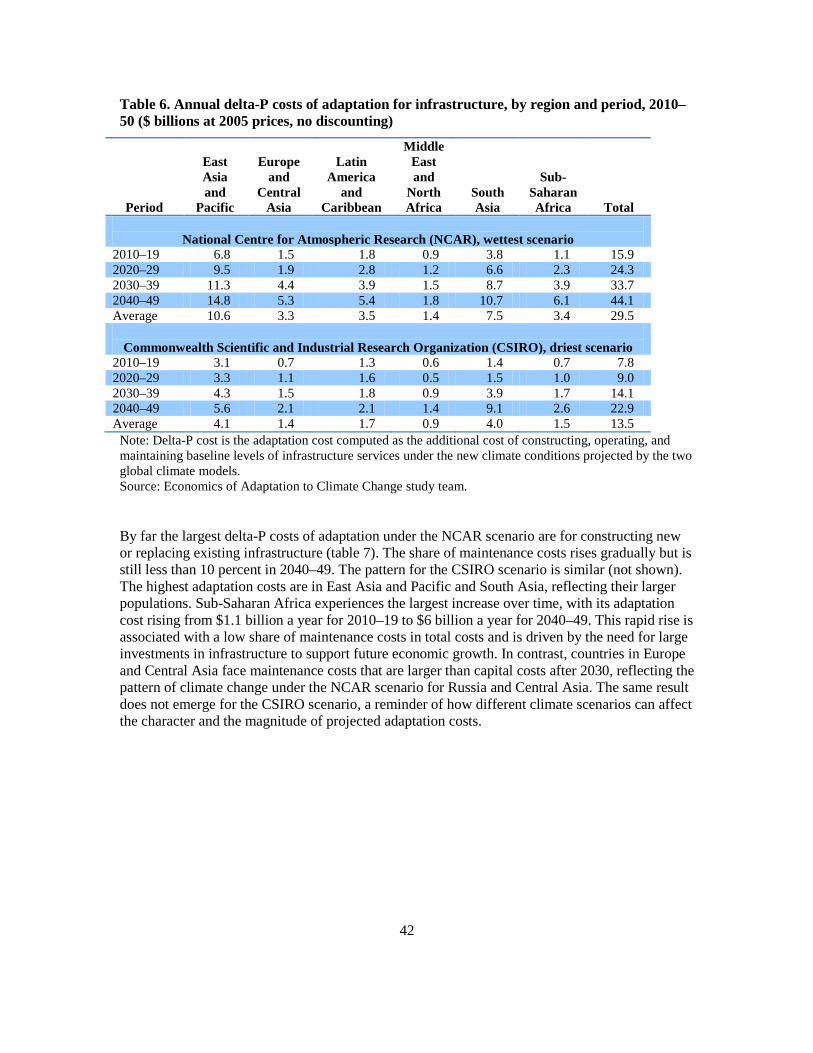
42

Table 6. Annual delta-P costs of adaptation for infrastructure, by region and period, 2010–50 ($ billions at 2005 prices, no discounting)

Period

East Asia and

Pacific

Europe and

Central Asia

Latin America

and Caribbean

Middle East and

North Africa

South Asia



2010–19 6.8 1.5 1.8 0.9 3.8 1.1 15.9 2020–29 9.5 1.9 2.8 1.2 6.6 2.3 24.3 2030–39 11.3 4.4 3.9 1.5 8.7 3.9 33.7 2040–49 14.8 5.3 5.4 1.8 10.7 6.1 44.1 Average 10.6 3.3 3.5 1.4 7.5 3.4 29.5

Commonwealth Scientific and Industrial Research Organization (CSIRO), driest scenario 2010–19 3.1 0.7 1.3 0.6 1.4 0.7 7.8 2020–29 3.3 1.1 1.6 0.5 1.5 1.0 9.0 2030–39 4.3 1.5 1.8 0.9 3.9 1.7 14.1 2040–49 5.6 2.1 2.1 1.4 9.1 2.6 22.9 Average 4.1 1.4 1.7 0.9 4.0 1.5 13.5

Note: Delta-P cost is the adaptation cost computed as the additional cost of constructing, operating, and maintaining baseline levels of infrastructure services under the new climate conditions projected by the two global climate models. Source: Economics of Adaptation to Climate Change study team. By far the largest delta-P costs of adaptation under the NCAR scenario are for constructing new or replacing existing infrastructure (table 7). The share of maintenance costs rises gradually but is still less than 10 percent in 2040–49. The pattern for the CSIRO scenario is similar (not shown). The highest adaptation costs are in East Asia and Pacific and South Asia, reflecting their larger populations. Sub-Saharan Africa experiences the largest increase over time, with its adaptation cost rising from $1.1 billion a year for 2010–19 to $6 billion a year for 2040–49. This rapid rise is associated with a low share of maintenance costs in total costs and is driven by the need for large investments in infrastructure to support future economic growth. In contrast, countries in Europe and Central Asia face maintenance costs that are larger than capital costs after 2030, reflecting the pattern of climate change under the NCAR scenario for Russia and Central Asia. The same result does not emerge for the CSIRO scenario, a reminder of how different climate scenarios can affect the character and the magnitude of projected adaptation costs.

43

Table 7. Breakdown of annual delta-P costs of adaptation for infrastructure for the National Centre for Atmospheric Research (NCAR) climate scenario, by region and cost type, 2010–2050 ($ billions at 2005 prices, no discounting)

Period and cost type

East Asia and

Pacific

Europe and

Central Asia

Latin America

and Caribbean

Middle East and

North Africa

South Asia


2010–19 Capital 6.7 1.2 1.8 0.9 3.8 1.1 15.5 Maintenance 0.1 0.2 0 0 0 0 0.3 Total 6.8 1.4 1.8 0.9 3.8 1.1 15.9 2020–29 Capital 9.3 1.7 2.7 1.2 6.5 2.3 23.7 Maintenance 0.2 0.2 0.1 0 0.1 0 0.7 Total 9.5 1.9 2.8 1.2 6.6 2.3 24.3 2030–39 Capital 11.1 1.9 3.8 1.3 8.6 3.9 30.6 Maintenance 0.3 2.5 0.2 0.2 0.1 0.1 3.4 Total 11.4 4.4 4.0 1.5 8.7 4.0 33.7 2040–49 Capital 14.1 2.3 5.0 1.5 10.4 5.9 39.2 Maintenance 0.7 3.0 0.4 0.2 0.2 0.1 4.6 Total 14.8 5.3 5.4 1.7 10.6 6.0 44.1 Note: Delta-P cost is the adaptation cost computed as the additional cost of constructing, operating, and maintaining baseline levels of infrastructure services under the new climate conditions projected by NCAR and CSIRO global climate models. Source: Economics of Adaptation to Climate Change study team. Urban infrastructure (urban drainage, public buildings, and similar assets) accounts for 54 percent of the delta-P adaptation cost over 2010–50, followed by roads (mainly paved roads) at 23 percent. (Box 11 describes some of the private adaptation costs for urban housing that are not covered by planned adaptation.) Networks and associated assets (power generation, electricity transmission and distribution, fixed telephone lines, water and sewage treatment) account for less than 9 percent of the estimated cost of adaptation even though they account for about 45 percent of total infrastructure costs.

For comparison, table 8 also shows the total costs of providing each type of infrastructure (not just climate proofing)—the baseline cost. The costs of adaptation are 4.6 percent of the total costs of infrastructure provision over the period for urban infrastructure, 2.3–2.1 percent for roads and other transport, and less than 1 percent for the other infrastructure categories. Overall, the adaptation cost is 1.6 percent of total infrastructure costs. These shares contrast with those of previous studies, which use ranges of 0.01 percent to 8 percent to estimate adaptation costs (see table 4, where equivalent parameters are obtained by multiplying percentage of climate sensitive new investments by percentage increases in costs) and fail to differentiate by type of asset. These differences in parameter values explain in part why the EACC estimates of adaptation costs for infrastructure ($15–30 billion a year) fall between the maximum and the minimum of past estimates ($2–67 billion a year; see table 4).

44

Table 8. Breakdown of delta-P costs of adaptation for the National Centre for Atmospheric Research (NCAR) climate scenario, by region and infrastructure category, 2010–50, ($ billions at 2005 prices, no discounting)

Infrastructure category and adaptation or baseline cost typea

East Asia and

Pacific

Europe and

Central Asia

Latin America

and Caribbean

Middle East and

North Africa

South Asia


Health and education Adaptation 1.1 0.7 0.4 0.2 0.5 0.1 3.0 Baseline 123.6 87.8 68 36.3 54.3 16.2 386.2 Other transport Adaptation 0.2 0.3 0.1 0.1 0.1 0.1 0.9 Baseline 9.6 16.2 5.6 1.8 4.7 3.7 41.6 Power and wires Adaptation 0.6 0.6 0.2 0.1 0.3 0.1 1.9 Baseline 164.3 108.8 62.9 25.9 82.8 21.3 466 Roads Adaptation 1.8 0.7 1 0.6 1.4 0.8 6.3 Baseline 60.1 47.9 43.1 23.4 57.2 36.5 268.2 Urban infrastructure Adaptation 6.6 0.8 1.6 0.3 4.9 2.3 16.5 Baseline 105.1 83.3 40.3 12.2 85.7 29 355.6 Water and sewers Adaptation 0.3 0.1 0.1 0 0.2 0 0.7 Baseline 140.7 61 63 26.5 67.8 23.4 382.4 All infrastructure Adaptation 10.6 3.3 3.5 1.3 7.4 3.4 29.5 Baseline 603.5 405.1 282.8 126.2 352.5 130.1 1900.2 Note: Delta-P cost is the adaptation cost computed as the additional cost of constructing, operating, and maintaining baseline levels of infrastructure services under the new climate conditions projected by the two global climate models. a. The baseline cost is defined as the sum of capital and maintenance expenditures over the lifetime of the asset.


Box 11. Urban housing and climate change

Planned adaptation costs do not account for the high adaptation costs of urban housing, which are largely individually provided. EACC estimates annual average household investments in urban housing in response to climate change at $2.3 billion (in 2005 dollars) per year in 2010, rising to $25.6 billion a year by 2050, under the CSIRO climate scenario. Under the NCAR scenario, annual costs rise even more, from an average of $4.4 billion a year in 2010 to $45.5 billion by 2050. Under both scenarios, costs are highest in East Asia and Pacific (followed by Latin America and the Caribbean under CSIRO and Europe and Central Asia under NCAR).

45

The costs of adaptation related to housing would be even higher if they also accounted for slums. Most informal settlements in developing countries share characteristics that intensify the vulnerability of their residents to climate change (Moser and Satterthwaite forthcoming). These include poorly constructed buildings; inadequate infrastructure; lack of safe drinking water, drainage, and sanitation services; and severe overcrowding with attendant public health impacts. Municipal governments often neglect or even criminalize such settlements, exacerbating the problem of underprovisioning of protective infrastructure and services. These factors combine with high concentrations of poor people with few assets to make slums especially vulnerable to flooding and other extreme events, which can lead to loss of lives and property and the spread of diseases such as malaria.

As discussed in the participatory scenario workshops, Ghana presents considerable challenges in adapting urban slums to climate change. Rural migrants to Accra and increasingly to Ghana’s secondary towns cluster in slums prone to overcrowding and poor sanitation. Workshop participants report that floods are more severe in these sprawling urban spaces of coastal Ghana than in inland towns, in part because of weak urban planning. Urbanization, especially in slums, increases the risk of climate-related disasters such as flooding and landslides, in part because natural ecosystem-based storm breaks and rain catchment areas are increasingly converted to public buildings and housing developments.

Thus far the analysis has assumed that climate change does not affect demand for infrastructure, but only the cost of providing it under the no-climate change scenario. However, climate change is likely to affect the demand for infrastructure services as well. For example, the optimal investment in roads would vary depending on whether climate change alters the structure of the economy and thus the location of economic activity, or more or higher dykes might be needed to cope with sea level rise and storm surges (see the discussion of adaptation cost for coastal zones). Called the delta-Q component of adaptation cost because it focuses on changes in the quantity of infrastructure required in response to changes in demand, this component is difficult to estimate, for reasons discussed in box 12, and in several cases it was also difficult to identify mechanisms that could explain counterintuitive results. Therefore, although estimates of delta-Q are presented in table 9, for illustrative purposes, they are not used to calculate adaptation costs for infrastructure assets. A comparison of infrastructure estimates with and without estimated changes in infrastructure demand indicates that the demand equations do not imply any simple relationships between climate and infrastructure demand (table 9). In most cases, the impact of climate change depends on interactions among per capita GDP, urbanization, and the range between maximum and minimum temperatures or precipitation. As a consequence, the predicted impact of climate change on demand for infrastructure by country ranges from –5 percent to +5 percent of baseline investment. The overall impact is negative in most large countries, with the exception of the Europe and Central Asia region, so the net quantity adjustment reduces the overall cost of adaptation by $19–22 billion a year for the two scenarios. This is equivalent to a reduction of about 1 percent of the baseline cost of infrastructure, demonstrating that small shifts in demand can have a very large impact on the total cost of adaptation. With the NCAR scenario, the net cost of adaptation for infrastructure declines from $29.5 billion a year to $7.3 billion a year when the delta-Q

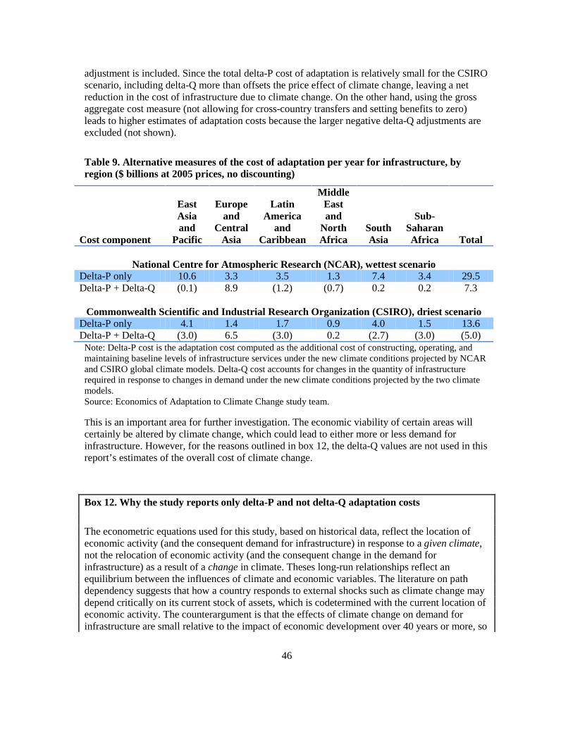
46

adjustment is included. Since the total delta-P cost of adaptation is relatively small for the CSIRO scenario, including delta-Q more than offsets the price effect of climate change, leaving a net reduction in the cost of infrastructure due to climate change. On the other hand, using the gross aggregate cost measure (not allowing for cross-country transfers and setting benefits to zero) leads to higher estimates of adaptation costs because the larger negative delta-Q adjustments are excluded (not shown).

Table 9. Alternative measures of the cost of adaptation per year for infrastructure, by region ($ billions at 2005 prices, no discounting)

Cost component

East Asia and

Pacific

Europe and

Central Asia

Latin America

and Caribbean

Middle East and

North Africa

South Asia



Delta-P only 10.6 3.3 3.5 1.3 7.4 3.4 29.5 Delta-P + Delta-Q (0.1) 8.9 (1.2) (0.7) 0.2 0.2 7.3


Delta-P only 4.1 1.4 1.7 0.9 4.0 1.5 13.6 Delta-P + Delta-Q (3.0) 6.5 (3.0) 0.2 (2.7) (3.0) (5.0)

Note: Delta-P cost is the adaptation cost computed as the additional cost of constructing, operating, and maintaining baseline levels of infrastructure services under the new climate conditions projected by NCAR and CSIRO global climate models. Delta-Q cost accounts for changes in the quantity of infrastructure required in response to changes in demand under the new climate conditions projected by the two climate models. Source: Economics of Adaptation to Climate Change study team.

This is an important area for further investigation. The economic viability of certain areas will certainly be altered by climate change, which could lead to either more or less demand for infrastructure. However, for the reasons outlined in box 12, the delta-Q values are not used in this report’s estimates of the overall cost of climate change.

Box 12. Why the study reports only delta-P and not delta-Q adaptation costs

The econometric equations used for this study, based on historical data, reflect the location of economic activity (and the consequent demand for infrastructure) in response to a given climate, not the relocation of economic activity (and the consequent change in the demand for infrastructure) as a result of a change in climate. Theses long-run relationships reflect an equilibrium between the influences of climate and economic variables. The literature on path dependency suggests that how a country responds to external shocks such as climate change may depend critically on its current stock of assets, which is codetermined with the current location of economic activity. The counterargument is that the effects of climate change on demand for infrastructure are small relative to the impact of economic development over 40 years or more, so

47

the effects of path dependency are swamped by the structural changes implied by the development baseline. Another hurdle concerns econometric specification. The data used for the analysis are a combination of time series and cross-country variables. Like other fixed country characteristics, climate variables are constant over time, so their influence has to be estimated from cross-country variation alone. Many studies rely on cross-country variation for key explanatory variables—for example, studies of the effects of governance and trade policy on economic growth. The cross-country variables help to explain a set of country fixed effects that are combined with the influence of factors (GDP per capita, population, urbanization, and so on) that vary across time and countries. The difficulty is that one or more climate variable might act as a proxy for country characteristics that influence the demand for infrastructure but that are not included in the analysis, so the coefficient on the climate variable will reflect both its direct influence on demand and its correlation with the omitted factor. Omitted variables are a potential problem in all econometric analysis, and it is impossible to demonstrate a negative—that the coefficients on the climate variables are not affected by omitted variables. The most that can be done is to include additional variables that may be better proxies for potential influences that cannot be included in the equations and to use specifications—such as interactions with time-varying factors—that reduce or eliminate correlation between omitted variables and climate variables. The influence of climate variables on demand for infrastructure remains an open area of research. There is ample evidence that some climate variables have an impact on specific types of infrastructure, such as temperature on energy demand or precipitation on water use. There is much less agreement on how these influences operate in the longer term and on whether the relationships can be extended to all categories of infrastructure. In view of these uncertainties, the final estimates of the costs of climate change exclude the delta-Q adjustments.

C oastal zones

Coastal zones, home to an ever-growing concentration of people and economic activity, are subject to several climate risks, including rising sea level and increased intensity of tropical storms and cyclones, making adaptation to climate change critical, particularly in small islands and deltaic countries (see box 13).

Box 13. Adaptation costs for deltaic countries and small islands states

Deltaic countries and small island states are particularly at risk for sea-level rise induced by climate change. For deltaic communities, ongoing subsidence and land conversion may exacerbate the effects of sea-level rise or extreme sea levels caused by intense storms. Small island states are vulnerable because of their small size, limited resource base, and geographic isolation.

Adaptation costs and residual damages for the medium sea-level rise scenario suggest that the costs of

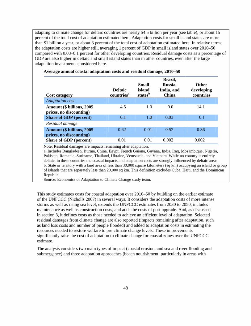
48

adapting to climate change for deltaic countries are nearly $4.5 billion per year (see table), or about 15 percent of the total cost of adaptation estimated here. Adaptation costs for small island states are more than $1 billion a year, or about 3 percent of the total cost of adaptation estimated here. In relative terms, the adaptation costs are higher still, averaging 1 percent of GDP in small island states over 2010–50 compared with 0.03–0.1 percent for other developing countries. Residual damage costs as a percentage of GDP are also higher in deltaic and small island states than in other countries, even after the large adaptation investments considered here.

Average annual coastal adaptation costs and residual damage, 2010–50

Cost category Deltaic

countriesa

Small island statesb

Brazil, Russia,

India, and China

Other developing countries

Adaptation cost Amount ($ billions, 2005 prices, no discounting)

4.5 1.0 9.0 14.1

Share of GDP (percent) 0.1 1.0 0.03 0.1 Residual damage Amount ($ billions, 2005 prices, no discounting)

0.62 0.01 0.52 0.36

Share of GDP (percent) 0.01 0.01 0.002 0.002 Note: Residual damages are impacts remaining after adaptation. a. Includes Bangladesh, Burma, China, Egypt, French Guiana, Guyana, India, Iraq, Mozambique, Nigeria, Pakistan, Romania, Suriname, Thailand, Ukraine, Venezuela, and Vietnam. While no country is entirely deltaic, in these countries the coastal impacts and adaptation costs are strongly influenced by deltaic areas. b. State or territory with a land area of less than 30,000 square kilometers (sq km) occupying an island or group of islands that are separately less than 20,000 sq km. This definition excludes Cuba, Haiti, and the Dominican Republic. Source: Economics of Adaptation to Climate Change study team.

This study estimates costs for coastal adaptation over 2010–50 by building on the earlier estimate of the UNFCCC (Nicholls 2007) in several ways. It considers the adaptation costs of more intense storms as well as rising sea level, extends the UNFCCC estimates from 2030 to 2050, includes maintenance as well as construction costs, and adds the costs of port upgrade. And, as discussed in section 3, it defines costs as those needed to achieve an efficient level of adaptation. Selected residual damages from climate change are also reported (impacts remaining after adaptation, such as land loss costs and number of people flooded) and added to adaptation costs in estimating the resources needed to restore welfare to pre-climate change levels. These improvements significantly raise the cost of adaptation to climate change for coastal zones over the UNFCCC estimate.

The analysis considers two main types of impact (coastal erosion, and sea and river flooding and submergence) and three adaptation approaches (beach nourishment, particularly in areas with

49

high tourism revenue; sea and river7

dike construction; and port upgrade). Impacts due to salinization and wetland loss are not considered (see box 14 for details).

Box 14. Coastal zone methodology

Adaptation costs for coastal zones are derived mainly from the Dynamic and Interactive Vulnerability Assessment (DIVA) model, based on 12,148 coastal segments that make up the world’s coast (except for Antarctica) and a linked database and set of interacting algorithms (MacFadden and others 2007; Nicholls and others 2007; Vafeidis and others 2008). The sea-level rise scenarios are downscaled with an estimate of the vertical land movement in each segment. The coastal erosion analysis considers only sandy coasts and takes account of the direct effect (Bruun effect) and indirect effects of sea-level rise, as well as beach nourishment where it occurs. The indirect effects occur at major estuaries and lagoons. The flooding analysis determines the flood areas for different return periods and extreme water levels, including the effects of dikes. Since empirical data on actual dike heights are not available at a global level, “optimum” dikes heights were estimated for the base year of 1995 using a demand for safety function.1 Dike heights are then upgraded according to projected sea-level rise to 2050. Increased flooding due to sea-level rise along the coastal-influenced reaches of major global rivers (identified in the DIVA database) is also considered. Damages are evaluated in terms of physical, social, and economic indicators such as land lost to erosion or submergence, the number of people expected to be subject to annual flooding, the number of people forced to migrate because of land loss, and the costs of this migration. DIVA implements the adaptation options according to complementary adaptation strategies. For beach nourishment, a cost-benefit adaptation strategy balances costs and benefits (damage avoided) of adaptation, including the tourist value of beaches. For dike building, the demand function for safety is applied over time, subject to population density. Dikes are built only when population density exceeds 1 person per square kilometer, with an increasing proportion of the recommended height being built as population density rises—for example, 98 percent of the dike height is built at densities of 1,000 people per square kilometer. The unit costs of beach nourishment, dikes, and port upgrades were derived from the global experience of Delft Hydraulics (now Deltares). For this analysis, DIVA was extended to include a sensitivity analysis of more intense tropical storms. This influences adaptation costs only for dikes. The maintenance costs of sea and river dikes and port upgrades globally are also computed outside DIVA. Port costs are based on a strategy of continuously raising existing port areas2 as sea levels rise. __________

7 This concerns the incremental costs of upgrading river dikes in coastal lowlands where sea-level rise will raise extreme water levels. Additional upgrade may be required if extreme river flows are increased, but this is not investigated here.

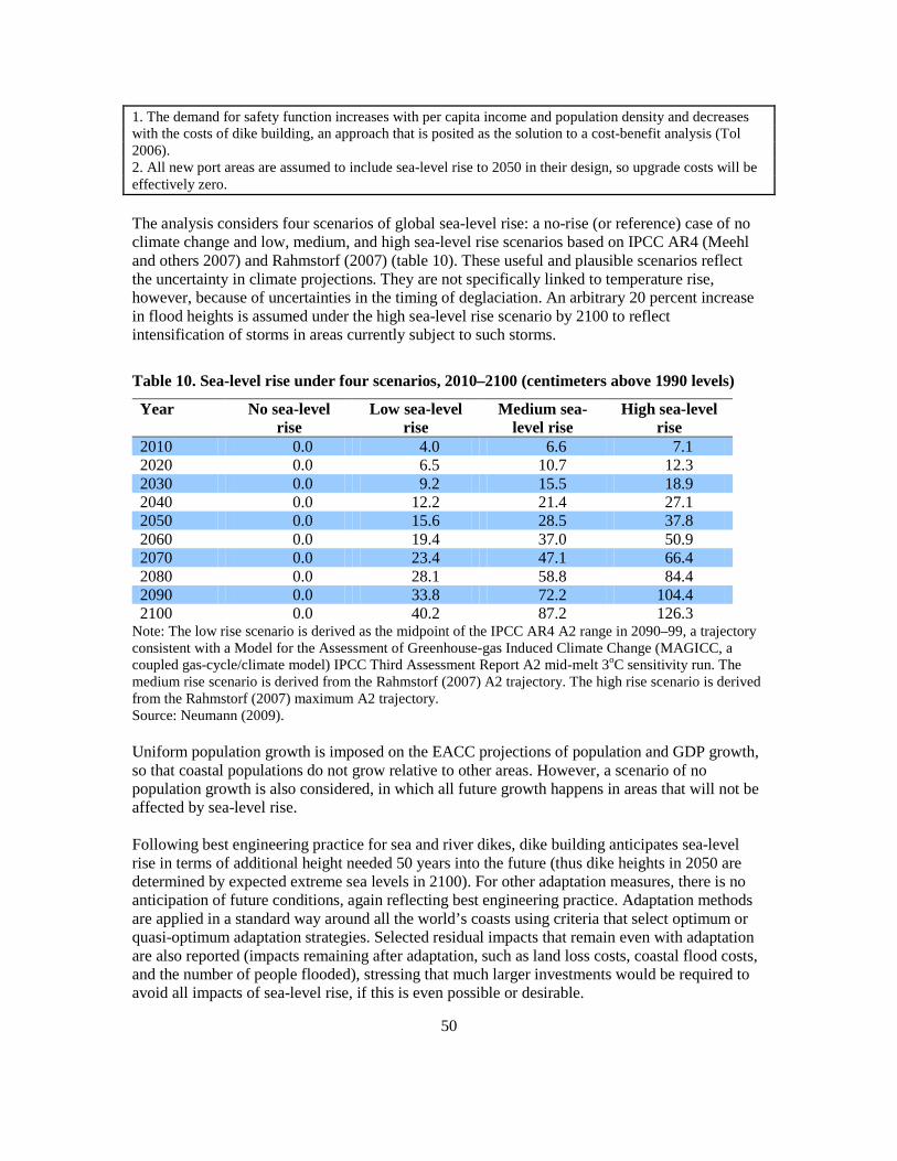
50

1. The demand for safety function increases with per capita income and population density and decreases with the costs of dike building, an approach that is posited as the solution to a cost-benefit analysis (Tol 2006). 2. All new port areas are assumed to include sea-level rise to 2050 in their design, so upgrade costs will be effectively zero. The analysis considers four scenarios of global sea-level rise: a no-rise (or reference) case of no climate change and low, medium, and high sea-level rise scenarios based on IPCC AR4 (Meehl and others 2007) and Rahmstorf (2007) (table 10). These useful and plausible scenarios reflect the uncertainty in climate projections. They are not specifically linked to temperature rise, however, because of uncertainties in the timing of deglaciation. An arbitrary 20 percent increase in flood heights is assumed under the high sea-level rise scenario by 2100 to reflect intensification of storms in areas currently subject to such storms.

Table 10. Sea-level rise under four scenarios, 2010–2100 (centimeters above 1990 levels)

Year No sea-level rise

Low sea-level rise

Medium sea-level rise

High sea-level rise

2010 0.0 4.0 6.6 7.1 2020 0.0 6.5 10.7 12.3 2030 0.0 9.2 15.5 18.9 2040 0.0 12.2 21.4 27.1 2050 0.0 15.6 28.5 37.8 2060 0.0 19.4 37.0 50.9 2070 0.0 23.4 47.1 66.4 2080 0.0 28.1 58.8 84.4 2090 0.0 33.8 72.2 104.4 2100 0.0 40.2 87.2 126.3

Note: The low rise scenario is derived as the midpoint of the IPCC AR4 A2 range in 2090–99, a trajectory consistent with a Model for the Assessment of Greenhouse-gas Induced Climate Change (MAGICC, a coupled gas-cycle/climate model) IPCC Third Assessment Report A2 mid-melt 3oC sensitivity run. The medium rise scenario is derived from the Rahmstorf (2007) A2 trajectory. The high rise scenario is derived from the Rahmstorf (2007) maximum A2 trajectory. Source: Neumann (2009). Uniform population growth is imposed on the EACC projections of population and GDP growth, so that coastal populations do not grow relative to other areas. However, a scenario of no population growth is also considered, in which all future growth happens in areas that will not be affected by sea-level rise. Following best engineering practice for sea and river dikes, dike building anticipates sea-level rise in terms of additional height needed 50 years into the future (thus dike heights in 2050 are determined by expected extreme sea levels in 2100). For other adaptation measures, there is no anticipation of future conditions, again reflecting best engineering practice. Adaptation methods are applied in a standard way around all the world’s coasts using criteria that select optimum or quasi-optimum adaptation strategies. Selected residual impacts that remain even with adaptation are also reported (impacts remaining after adaptation, such as land loss costs, coastal flood costs, and the number of people flooded), stressing that much larger investments would be required to avoid all impacts of sea-level rise, if this is even possible or desirable.

51

Table 11. Annual costs of adaptation for coastal zone protection, by scenario and cost component, 2010–50 ($ billions at 2005 prices, no discounting)

Coastal zone cost component

Low sea-level rise

Medium sea-level rise

High sea-level rise

High sea-level rise with cyclones

Beach nourishment 1.7 3.3 4.5 4.5 River dikes 0.2 0.4 0.6 0.6 Sea dikes 10.7 24.6 36.7 39.1 Port upgrades 0.2 0.4 0.5 0.5 Residual damagesa 0.7 1.5 2 2 Total 13.5 30.2 44.3 46.7

a. Includes impacts remaining after adaptation, such as land loss, coastal flooding, and number of people flooded. Source: Economics of Adaptation to Climate Change study team. Coastal adaptation costs are substantial and vary with the magnitude of sea-level rise (table 11), making it essential for policymakers to plan while accounting for the uncertainty. Flooding dominates both the adaptation costs (of building dikes) and the costs of damages due to the residual risk. Sea-level rise does not have a large effect on the size of residual damages—the main effect is an increased investment in adaptation. An analysis of how adaptation costs and residual damages are distributed for the medium sea-level rise scenario indicates that Latin American and the Caribbean and East Asia and Pacific together account for some two thirds of the total cost of adaptation (table 12). Deltaic countries and small island states are particularly at risk (see box 13). Increased tropical storm intensity does not raise annual costs substantially, and targeting future population growth outside the coastal flood plain does not reduce costs substantially, as the existing development already creates a substantial need for protection.

Clearly, a wider range of adaptation options than considered in DIVA are available in practice, including retreating from coastal zones and accommodating higher water levels by raising buildings above flood levels. These steps could reduce the need for protection measures and could lead to lower adaptation costs than those estimated here (these softer measures are very difficult to cost, which is why that was not done). Realizing these benefits will require long-term strategic planning and more integration across coastal planning and management. Few if any countries have this capacity today, and strengthening institutional capacity for integrated coastal management would seem a prudent response to climate change (also yielding benefits in other areas).

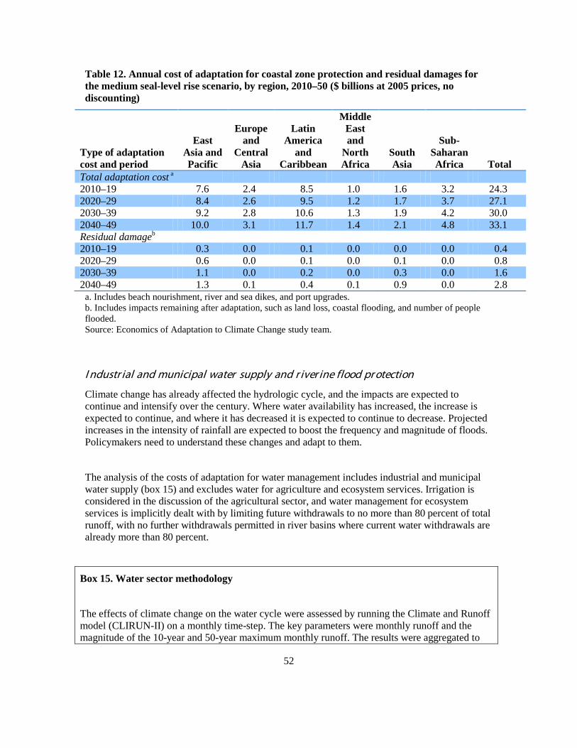
52

Table 12. Annual cost of adaptation for coastal zone protection and residual damages for the medium seal-level rise scenario, by region, 2010–50 ($ billions at 2005 prices, no discounting)

Type of adaptation cost and period

East Asia and Pacific

Europe and

Central Asia

Latin America

and Caribbean

Middle East and

North Africa

South Asia


Total adaptation cost a 2010–19 7.6 2.4 8.5 1.0 1.6 3.2 24.3 2020–29 8.4 2.6 9.5 1.2 1.7 3.7 27.1 2030–39 9.2 2.8 10.6 1.3 1.9 4.2 30.0 2040–49 10.0 3.1 11.7 1.4 2.1 4.8 33.1 Residual damageb 2010–19 0.3 0.0 0.1 0.0 0.0 0.0 0.4 2020–29 0.6 0.0 0.1 0.0 0.1 0.0 0.8 2030–39 1.1 0.0 0.2 0.0 0.3 0.0 1.6 2040–49 1.3 0.1 0.4 0.1 0.9 0.0 2.8

a. Includes beach nourishment, river and sea dikes, and port upgrades. b. Includes impacts remaining after adaptation, such as land loss, coastal flooding, and number of people flooded. Source: Economics of Adaptation to Climate Change study team.

I ndustr ial and municipal water supply and r iver ine flood pr otection

Climate change has already affected the hydrologic cycle, and the impacts are expected to continue and intensify over the century. Where water availability has increased, the increase is expected to continue, and where it has decreased it is expected to continue to decrease. Projected increases in the intensity of rainfall are expected to boost the frequency and magnitude of floods. Policymakers need to understand these changes and adapt to them.

The analysis of the costs of adaptation for water management includes industrial and municipal water supply (box 15) and excludes water for agriculture and ecosystem services. Irrigation is considered in the discussion of the agricultural sector, and water management for ecosystem services is implicitly dealt with by limiting future withdrawals to no more than 80 percent of total runoff, with no further withdrawals permitted in river basins where current water withdrawals are already more than 80 percent.

Box 15. Water sector methodology

The effects of climate change on the water cycle were assessed by running the Climate and Runoff model (CLIRUN-II) on a monthly time-step. The key parameters were monthly runoff and the magnitude of the 10-year and 50-year maximum monthly runoff. The results were aggregated to

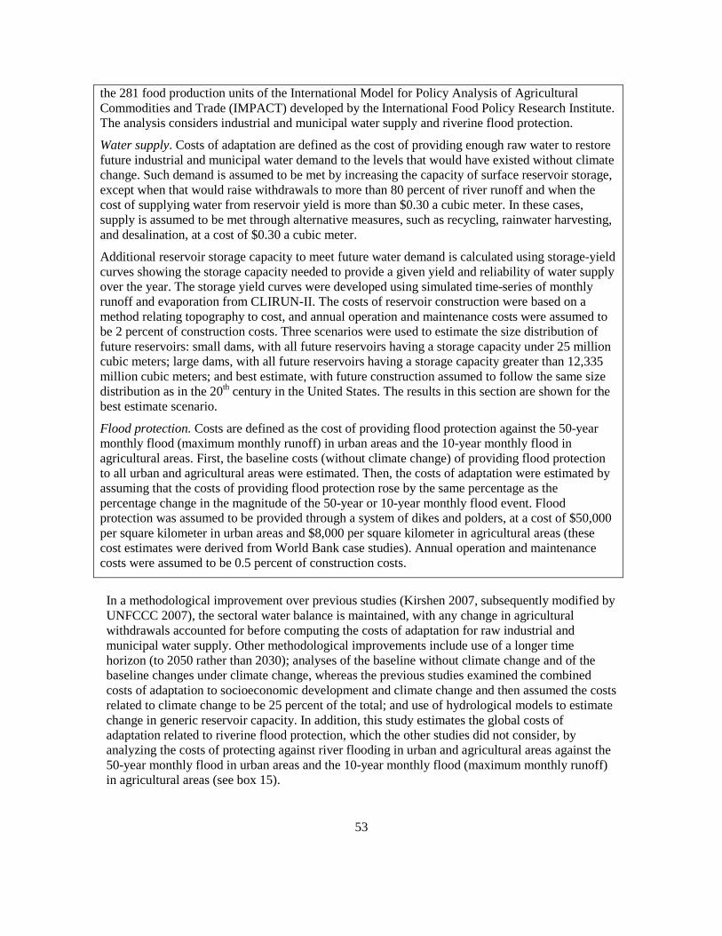
53

the 281 food production units of the International Model for Policy Analysis of Agricultural Commodities and Trade (IMPACT) developed by the International Food Policy Research Institute. The analysis considers industrial and municipal water supply and riverine flood protection.

Water supply. Costs of adaptation are defined as the cost of providing enough raw water to restore future industrial and municipal water demand to the levels that would have existed without climate change. Such demand is assumed to be met by increasing the capacity of surface reservoir storage, except when that would raise withdrawals to more than 80 percent of river runoff and when the cost of supplying water from reservoir yield is more than $0.30 a cubic meter. In these cases, supply is assumed to be met through alternative measures, such as recycling, rainwater harvesting, and desalination, at a cost of $0.30 a cubic meter.

Additional reservoir storage capacity to meet future water demand is calculated using storage-yield curves showing the storage capacity needed to provide a given yield and reliability of water supply over the year. The storage yield curves were developed using simulated time-series of monthly runoff and evaporation from CLIRUN-II. The costs of reservoir construction were based on a method relating topography to cost, and annual operation and maintenance costs were assumed to be 2 percent of construction costs. Three scenarios were used to estimate the size distribution of future reservoirs: small dams, with all future reservoirs having a storage capacity under 25 million cubic meters; large dams, with all future reservoirs having a storage capacity greater than 12,335 million cubic meters; and best estimate, with future construction assumed to follow the same size distribution as in the 20th century in the United States. The results in this section are shown for the best estimate scenario.

Flood protection. Costs are defined as the cost of providing flood protection against the 50-year monthly flood (maximum monthly runoff) in urban areas and the 10-year monthly flood in agricultural areas. First, the baseline costs (without climate change) of providing flood protection to all urban and agricultural areas were estimated. Then, the costs of adaptation were estimated by assuming that the costs of providing flood protection rose by the same percentage as the percentage change in the magnitude of the 50-year or 10-year monthly flood event. Flood protection was assumed to be provided through a system of dikes and polders, at a cost of $50,000 per square kilometer in urban areas and $8,000 per square kilometer in agricultural areas (these cost estimates were derived from World Bank case studies). Annual operation and maintenance costs were assumed to be 0.5 percent of construction costs.

In a methodological improvement over previous studies (Kirshen 2007, subsequently modified by UNFCCC 2007), the sectoral water balance is maintained, with any change in agricultural withdrawals accounted for before computing the costs of adaptation for raw industrial and municipal water supply. Other methodological improvements include use of a longer time horizon (to 2050 rather than 2030); analyses of the baseline without climate change and of the baseline changes under climate change, whereas the previous studies examined the combined costs of adaptation to socioeconomic development and climate change and then assumed the costs related to climate change to be 25 percent of the total; and use of hydrological models to estimate change in generic reservoir capacity. In addition, this study estimates the global costs of adaptation related to riverine flood protection, which the other studies did not consider, by analyzing the costs of protecting against river flooding in urban and agricultural areas against the 50-year monthly flood in urban areas and the 10-year monthly flood (maximum monthly runoff) in agricultural areas (see box 15).

54

Table 13. Gross and net annual adaptation costs for water supply and riverine flood protection, by region, 2010–50 ($ billions at 2005 prices, no discounting)

Type of cost calculation and protection category

East Asia and

Pacific

Europe and

Central Asia

Latin America

and Caribbean

Middle East and

North Africa

South Asia


National Centre for Atmospheric Research (NCAR), wettest scenario Gross Flood protection 0.9 1.7 1.0 0.2 1.1 0.4 5.3 Water supply 3.1 1.7 5.3 0.5 1.8 6.2 18.6 Total 4.0 3.4 6.3 0.7 2.9 6.6 23.9 Net Flood protection 0.8 1.4 0.3 –0.2 1.0 0.3 3.6 Water supply 0.3 0.9 5.2 0.0 –2.3 5.9 10.0 Total 1.1 2.3 5.5 –0.2 –1.3 6.2 13.3 Commonwealth Scientific and Industrial Research Organization (CSIRO), driest scenario

Gross Flood protection 1.6 0.9 2.0 0.6 1.7 0.2 7.0 Water supply 2.1 0.5 2.9 0.2 5.9 7.6 19.2 Total 3.7 1.4 4.9 0.8 7.6 7.8 26.2 Net Flood protection 1.6 0.6 1.7 0.5 1.6 –0.2 5.8 Water supply 0.6 –0.3 1.5 –0.4 2.4 7.3 11.1 Total 2.2 0.3 3.2 0.1 4.0 7.1 16.9

Note: Gross costs set negative values to zero for sector protection in any country with negative costs. Net costs are the pooled costs without restrictions on pooling across country borders (positive and negative values are treated symmetrically).


Adaptation costs for industrial and municipal raw water supply are higher for the CSIRO simulations, with its drier global mean conditions, than for the NCAR simulations, with its wetter conditions (table 13 and map 3), because more reservoir storage capacity is required to provide the same yield. The adaptation costs for riverine flood protection are also greater for the CSIRO scenario because the model simulates a larger increase in the magnitude of the 10-year and 50-year monthly flood events than does the NCAR scenario, despite relatively drier mean conditions. The highest costs are in Sub-Saharan Africa under both climate scenarios. Latin America and the Caribbean also sustain high costs under both models, and South Asia sustains high costs under CSIRO because these regions experience the largest percentage decline in mean runoff (see map 3). The gross costs of adaptation are significantly greater than the net costs, especially for water supply: $23.9 billion gross and $13.3 billion net annual cost under NCAR and $26.2 billion gross and $16.9 billion net annual cost under CSIRO. These differences are driven mainly by the decreased need for storage capacity in South Asia and East Asia and Pacific under both scenarios because of increased mean runoff (see map 3).

55

Map 3. Change in mean water runoff under the Commonwealth Scientific and Industrial Research Organization and National Centre for Atmospheric Research global climate scenarios, 2000–50


scenario National Centre for Atmospheric Research

(NCAR), wettest scenario

Note: The Economics of Adaptation to Climate Change study team acknowledges the Program for Climate Model Diagnosis and Intercomparison and the World Climate Research Programme's (WCRP) Working Group on Coupled Modelling for their roles in making available the WCRP’s Coupled Model Intercomparison Project phase 3 (CMIP3) multimodel dataset. Support of this dataset is provided by the Office of Science, U.S. Department of Energy.


As do most sectoral studies of global adaptation costs, this study focuses on hard adaptation measures, which are easier to cost than behavioral measures. There is no implication that these are the best measures for adaptation. Ideally, adaptation options to ensure water supply during average and drought conditions should integrate strategies on both demand and supply sides. While demand-side adaptations are not explicitly costed in this study (demand projections already account for some increase in efficiencies over time, so this could lead to double counting), there is wide scope for economizing on water consumption (see, for example, Zhou and Tol 2005). Adaptation options for flood protection can reduce either the probability of flood events or their

56

magnitude (reducing flood hazard) or the impacts of floods. In both cases, adaptation should consider structural and nonstructural measures that address both flood probability and impact.

A gr icultur e

The analysis of agriculture brings together, for the first time, detailed biophysical modeling of crop growth under climate change with the world’s most detailed global partial equilibrium agricultural model to estimate the costs of adaptation for returning the number of malnourished children to pre-climate change levels. One of the few earlier estimates of adaptation costs for agriculture takes a simpler approach, assuming that an arbitrary 10 percent increase in research and extension funding and a 2 percent increase in capital infrastructure costs are needed by 2030 to adapt to climate change (UNFCCC 2007). Also, the UNFCCC estimate includes no explicit link to climate impacts or any accounting for autonomous (personal) adaptation. The analysis of agricultural adaptation costs uses the International Food Policy Research Institute’s (IFPRI) International Model for Policy Analysis of Agricultural Commodities and Trade (IMPACT) to incorporate the direct impacts of climate change on agricultural production (yields and crop area) and the indirect effects through food prices and trade on calorie availability and the number of malnourished children (see box 16). IMPACT includes 32 crops and livestock commodities, including cereals, soybeans, roots and tubers, meats, milk, eggs, oilseeds, oilcakes and meals, sugar, and fruits and vegetables. Changes in the number of malnourished children between 2050 and 2000 without climate change are compared to changes with climate change to determine costs of adaptation.

Box 16. Agriculture sector methodology

Climate change affects agriculture through changes in yields and in areas planted. Farmers respond by changing their management practices. The resulting production effects work their way through agricultural markets, affecting prices. Consumers respond by changing consumption patterns. When prices rise, consumption falls and the number of malnourished children rises. Adaptation expenditures on productivity enhancing investments can offset these impacts of climate change. The biological effects of climate change are modeled with the Decision Support System for Agrotechnology Transfer (DSSAT) crop modeling program, assessing yield and area effects for five major commodities at 0.5 degree resolution. The DSSAT model includes a carbon dioxide fertilization effect of 369 parts per million (ppm) atmospheric concentration, reflecting recent research suggesting that fertilization effects are much weaker in the field than in the laboratory. Using a 532 ppm value reduces the costs of adaptation by less than 10 percent. The productivity effects of climate change are aggregated to 32 crops and 281 food production units of the International Food Policy Research Institute’s International Model for Policy Analysis of Agricultural Commodities and Trade. Growth in crop production in each country is determined by crop and input prices, exogenous rates of productivity growth and area expansion, investment in irrigation, and water availability. Demand is modeled as a function of prices, income, and population growth and has four components: food, feed, biofuels feedstock, and other uses. The model links national agricultural markets through international trade. World agricultural commodity prices are determined annually at levels that clear international markets.

57

Costs of adaptation are measured against the human well-being measure of malnutrition in preschool children, a highly vulnerable group. The number of malnourished children is determined in part by per calorie availability but also by access to clean drinking water and maternal education. Investments in agricultural research, roads, and irrigation increase agricultural productivity under climate change, increasing calorie availability and reducing child malnutrition estimates. The costs of adaptation for agriculture are calculated solely from the perspective of the agriculture sector, so the starting point is investment and asset stocks in the base year (2000). Thus, the estimates of investments in research, irrigation, and rural roads do not take account of overlaps in spending on these activities or assets with the baseline growth or of adaptation costs for other sectors, such as infrastructure and water resources management. This is an unavoidable consequence of estimating the cost of adaptation for each sector separately and in parallel. For rural roads, an attempt was made to eliminate overlapping expenditures in compiling the consolidated estimates of the costs of adaptation for developing countries in table 24. The baseline provision of rural roads up to 2050 used to estimate costs of adaptation is adjusted to take account of the additional length of rural roads consistent with the baseline projections for road investment. This adjustment reduces the investment in rural roads included in the cost of adaptation for agriculture by about 80–85 percent for the two climate scenarios. The adjustment for these overlaps amounts to $2.0–2.2 billion a year averaged over the full period. Changes in temperature and precipitation in the NCAR and CSIRO climate scenarios have strong negative effects on crop yields and production. Irrigated and rainfed wheat and irrigated rice are especially hard hit. South Asia experiences the biggest loss in production, and developing countries fare worse than developed countries for almost all crops under both scenarios. These productivity impacts, even after accounting for autonomous adjustments through changes in, say, input and crop mix (see box 17 on some private adaptation measures in agriculture in some case study countries), lead to dramatic impacts on trade flows (another form of autonomous adjustment). Without climate change, developed country net exports rise from 83.3 million tons to 105.8 million tons between 2000 and 2050—a 27 percent increase. South Asia switches from a net exporter to a net importer, and East Asia and Pacific and Sub-Saharan African imports rise considerably (table 14 and figure 3). Developed country exports rise 28 percent under the NCAR scenario and a dramatic 75 percent under the CSIRO scenario compared with 2000 levels (not shown). South Asia becomes a much larger importer of food under both scenarios than under baseline conditions of no climate change, East Asia and Pacific becomes a net exporter of food under the NCAR scenario, and Europe and Central Asian exports and Sub-Saharan African imports fall substantially under both scenarios. Climate change has a smaller impact on meat trade.

Box 17. Private adaptation in agriculture and areas needing policy attention

Farmers in Sub-Saharan Africa are already adapting to increasing rainfall variability and higher temperatures by shifting sowing dates and changing crop mix or plot location. In Ethiopia and Ghana, farmers in focus groups reported on significant changes in the start of the rainy season and in the length and intensity of rainfall. In Ghana, male and female farmers reported that they

58

had responded to the variable precipitation and higher temperatures by planting drought- and heat-resistant crops, selecting crops with a short gestation period, planting vegetables along river banks for easier access to water, shifting planting dates forward or backward, and sowing half the plot later to spread the risk of early or late rains. Farmers in Bolivia also note adaptations in agricultural practices with climate change, including using new seed varieties and turning over pastureland to cropland in the Alturas (highlands), where temperatures have risen.

In these settings, the coping strategies of the poorest farmers are even more constrained under conditions of climate change, leaving them less room for implementing adaptation responses. For example, a focus group of vulnerable women in rural Ghana noted that the Nandana (poorer people) lack collateral for loans and thus have to beg other community members for leftover seeds to sow. They are therefore the last to sow their crops and miss crucial sowing dates.

In all the case study countries, land was identified as a policy area with an important bearing on potential climate adaptation activities. Land tenure systems affect poverty outcomes directly. For example, priority adaptation investments are expected to include investments in water infrastructure (including irrigation) to cope with growing freshwater scarcity. However, the greatest impacts of such irrigation investments on poverty reduction have been found in countries with low levels of inequality in land holdings (Hussain 2005). Land inequity is greatest for women. In Tetauku, Ghana, members of an EACC focus group discussion on the elderly declared that “Women do not own land; even their own children who are boys have more inheritance rights than their mothers.” An elderly man added that “even if you are blind or physically challenged you would always have a piece of land as long as you are a boy or a man.”

Table 14. Value of net cereal trade by region, with and without climate change and with and without adaptation investments, by region, 2000 and 2050 ($ millions at 2000 prices, no discounting)

Region 2000

2050

Without climate change

National Centre for Atmospheric Research


Commonwealth Scientific and Industrial Research Organization (CSIRO),

driest scenario Without

adaptation With

adaptation Without

adaptation With

adaptation South Asia 2,589 –2,238 –14,727 –11,700 –14,927 –11,406 East Asia and Pacific –1,795 –7,980 6,530 7,304 –8,879 –4,220 Europe and Central Asia

750 24,276 6,662 6,381 14,377 12,789

Latin America and Caribbean

–1,246 –6,027 480 –1,874 –342 –3,094

Middle East and North Africa

–5,600 –12,654 –17,703 –12,985 –17,723 –13,233

Sub-Saharan Africa –2,995 –12,870 –11,153 –10,560 –10,914 –10,392 Developing countries –8,500 –18,184 –30,733 –24,163 –39,219 –30,273


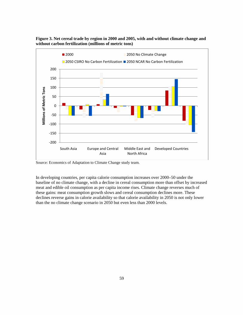
59

Figure 3. Net cereal trade by region in 2000 and 2005, with and without climate change and without carbon fertilization (millions of metric tons)

Source: Economics of Adaptation to Climate Change study team. In developing countries, per capita calorie consumption increases over 2000–50 under the baseline of no climate change, with a decline in cereal consumption more than offset by increased meat and edible oil consumption as per capita income rises. Climate change reverses much of these gains: meat consumption growth slows and cereal consumption declines more. These declines reverse gains in calorie availability so that calorie availability in 2050 is not only lower than the no climate change scenario in 2050 but even less than 2000 levels.

-200

-150

-100

-50

0

50

100

150

200

South Asia Europe and Central Asia


Developed Countries

Mill

ions

of M

etri

c To

ns

2000 2050 No Climate Change

2050 CSIRO No Carbon Fertilization 2050 NCAR No Carbon Fertilization

60

Table 15. Adaptation costs in agriculture—number of malnourished children under age five for three scenarios, by region, 2000 and 2050 (millions)

Region 2000

2050

Without climate change


Research (NCAR), wettest

scenario

Commonwealth Scientific and Industrial Research Organization

(CSIRO), driest scenario

South Asia Number Percent

75.6 —

52.3 31

59.1 22

58.6 22

East Asia and Pacific Number Percent

23.8 —

10.1 58

14.5 39

14.3 40

Europe and Central Asia Number Percent

4.1 —

2.7 34

3.7 10

3.7 10


Number Percent

7.5 —

5.0 35

6.4 17

6.4 17


Number Percent

3.5 —

1.1 69

2.1 40

2.0 43

Sub-Saharan Africa Number Percent

32.7 —

41.7 +28

52.2 +60

52.1 +59

Total Number Percent

110.63 25

136.72 7

135.78 8


The decline in calorie availability brought about by climate change also increases the number of malnourished children (table 15). Without climate change, income and agricultural productivity gains result in large declines in the number of malnourished children in all parts of the developing world except Sub Saharan Africa, where the absolute numbers increase from 33 million in 2000 to 42 million in 2050. Climate change eliminates most of these improvements. In South Asia, the numbers of malnourished children in 2050 rises from 52 million without climate change to 59 million with climate change. The large impact in agriculture worldwide suggests that public investments (planned adaptation) of about $8 billion annually are needed between 2010 and 2050 to restore development gains in nutritional levels, especially for children, to levels without climate change (see table 14). The types of adaptations considered include more spending on research and extension, expansion of irrigated areas along with efficiency improvements, and expansion of rural road networks for lower cost access to inputs and higher farm-gate prices. Investment needs in Sub-Saharan Africa

61

dominate (mainly for rural roads), accounting for about a third of the total. South Asia and East Asia and Pacific also need large investments, mainly in irrigation efficiency improvements. Differences between gross and net costs of adaptation are small.

Adaptation costs of planned or public investments do not, by definition, capture costs associated with autonomous adaptation, particularly important in agriculture. One component of autonomous adaptation costs in agriculture is changes in net trade values. As shown in table 14, without climate change, cereal imports for developing countries roughly double between 2000 and 2050. With climate change, cereal imports roughly triple, and the drier CSIRO scenario makes trade imbalances larger than does the NCAR scenario. Agricultural productivity investments of the type needed to meet the child nutrition adaptation also reduce net cereal imports for developing countries, although not by much.

62

Table 16. Annual cost of adaptation for agriculture—counteracting the effects of climate change on children’s nutrition levels, by region and cost type, 2010–50 ($ billions at 2005 prices, no discounting)

Cost type and investment category


Europe and

Central Asia

Latin America

and Caribbean

Middle East and

North Africa

South Asia

Sub-Sahara

n Africa Total

National Centre for Atmospheric Research (NCAR), wettest scenario Gross Agricultural

research 0.2 0.1 0.4 0.2 0.2 0.3 1.4 Irrigation

efficiency 0.8 0.1 0.1 0.1 1.1 0.2 2.4 Irrigation

expansion 0.0 0.0 0.0 0.0 0.4 0.6 1.0 Roads 0.2 0.0 0.6 0.0 0.0 2.2 3.0 Total 1.1 0.2 1.2 0.3 1.7 3.3 7.9 Net Agricultural

research 0.2 0.1 0.4 0.2 0.2 0.3 1.3 Irrigation

efficiency 0.8 0.1 0.1 0.1 1.1 0.2 2.4 Irrigation

expansion 0.0 0.0 0.0 0.0 0.4 0.6 1.0 Roads 0.1 0.0 0.6 0.0 0.0 2.2 2.9 Total 1.0 0.2 1.2 0.2 1.7 3.3 7.6

Commonwealth Scientific and Industrial Research Organization (CSIRO), driest scenario Gross Agricultural research 0.2 0.1 0.4 0.2 0.2 0.3 1.4 Irrigation efficiency 0.7 0.1 0.1 0.1 1.1 0.2 2.4 Irrigation expansion 0.0 0.0 0.0 0.0 0.4 0.6 1.0 Roads 0.2 0.0 0.8 0.0 0.0 2.1 3.1 Total 1.1 0.3 1.3 0.3 1.7 3.2 7.9 Net Agricultural research 0.2 0.1 0.4 0.2 0.2 0.3 1.4 Irrigation efficiency 0.7 0.1 0.1 0.1 1.1 0.2 2.4 Irrigation expansion 0.0 0.0 0.0 0.0 0.4 0.6 1.0 Roads 0.1 0.0 0.8 0.0 0.0 2.1 3.0 Total 1.1 0.2 1.3 0.3 1.7 3.2 7.7


63

F isher ies

This is the first study to establish the costs of adaptation to climate change in the fisheries sector. The analysis begins by detailing the likely impact of climate change on the productivity of marine fisheries (more than 1,000 species) and, through that, on landed catch values and household incomes. Adaptation costs are then estimated as the costs of restoring these revenue indicators to levels that would have prevailed in the absence of climate change (see box 18). Lack of readily available data precludes the use of a more direct measure of welfare, as with calorie intake for agriculture. Data limitations also restrict the analysis to marine capture fisheries, leaving out inland fisheries and aquaculture. Marine capture fisheries constitute more than half of total global fisheries values and support large numbers of economically vulnerable people in coastal communities.

Box 18. Fisheries sector methodology

Climate change is likely to alter ocean conditions, particularly water temperature, ocean currents, upwelling, and biogeochemistry, leading to productivity shocks for marine fisheries (IPCC 2007; Diaz and Rosenberg 2008). Other studies have documented shifts in species distribution (Perry and others 2005; Dulvy and others 2008) and growth rates (Thresher and others 2007) as a result of changes in ocean temperatures. Climate change may also alter the phenology of marine organisms, creating mismatches between prey availability and predator requirements and leading to coral bleaching and habitat loss for reef-associated fish species (Sumaila and Chaeung 2008). To account for distributional, productivity, and biogeochemical effects, a two-step process is used to establish climate change impacts on fish catches. First, potential losses and gains in fish catches due to the redistribution of fish biomass and changes in primary production are determined under various climate change scenarios for all maritime countries and the high seas. These impacts are then modified by including the potential catch impacts in climate change vulnerable hot-spots, based on knowledge of the locations of different fish species. Potential effects of climate change on these areas include acidification of the oceans from higher carbon dioxide levels, loss of coral reef from ocean warming and acidification, and other changes in ocean biogeochemistry, such as oxygen levels. And second, potential losses and gains in landed catch values or gross revenues and household incomes from global fisheries under different climate change and baseline scenarios are estimated. Because of data limitations, losses in landed catches values are used as estimates of adaptation costs. The impacts of climate change on marine fisheries occur through changes in primary productivity and shifts in species distributions and through acidification of the oceans (from higher carbon dioxide levels) and climate change-induced losses of critical habitats, such as degradation of coral reefs through coral bleaching. Three scenarios are examined that reflect these impacts. All three scenarios assume changes in primary productivity and shifts in species distribution due to climate change. The less intensive scenario in addition assumes a 10 percent catch reduction due to habitat losses by 2050 compared with the baseline that maintains 2010 stock levels out to 2050,

64

the more intensive scenario assumes a 30 percent catch reduction due to habitat losses, and the overexploitation scenario assumes a 40 percent reduction in 2010 stock levels by 2050. . Climate change is predicted to lead to losses in landed catch values or gross fisheries revenues of $10–31 billion globally by 2050 and $7–19 billion for developing countries (table 17). East Asia and Pacific is projected to experience the largest losses. Losses are also considerable in high seas areas beyond individual countries’ exclusive economic zones.

Table 17. Loss in landed values of fish catches under three scenarios, 2050 ($ billions at 2005 prices, no discounting)

Country group and region Less intensive More intensive Overexploitation Global 16.75 31.31 9.64 Developed countries 4.13 8.07 2.27 Developing countries 11.19 18.77 7.02 High seas 1.43 4.47 0.35 Region South Asia 1.37 2.22 0.87 East Asia and Pacific 7.02 10.94 4.63 Europe and Central Asia 0.32 1.31 –0.01 Latin America and Caribbean 1.21 2.17 0.73 Middle East and North Africa 0.61 0.84 0.43 Sub-Saharan Africa 0.44 0.96 0.21 Other developing countries3 0.22 0.34 0.16

Note: The less intensive scenario assumes a 10 percent reduction by 2050 in annual catches compared with the baseline, the more intensive assumes a 30 percent reduction, and overexploitation assumes a 40 percent reduction.


Governments have implemented various measures to manage fisheries, both to conserve fish stocks and to help communities that depend on fishery resources adapt to changes caused by overfishing and other factors. Measures include buybacks, transferable quotas, and investments in alternative sources of employment and income. Adaptation to climate change is likely to involve an extension of such policies with a focus on providing alternative sources of income in fishing communities to lessen the dependence on fishery resources. But only limited information is available on the potential costs of adaptation. The best documented are measures responding to the catastrophic decline in cod stock off Newfoundland, Canada, where the cost was equivalent to $4,950 per ton of reduced catches at 2005 prices. Because of the paucity of data, adaptation costs were estimated as the damages caused by climate change or reductions in landed catch values induced by climate change. No attempt was made to allocate the loss associated with fisheries in the high seas. Most of this loss will fall on the fishery sectors of developed countries, so this omission does not have much impact on the overall cost of adaptation. Adaptation costs are highest under the more-intensive scenario and not under the overexploitation scenario, because there are fewer fish under the overexploitation scenario to be affected by climate change (table 18). Regionally, nearly two-thirds of the costs of adaptation is incurred in East Asia and Pacific.

65

Table 18. Annual cost of adaptation for fisheries—loss in landed catch values, by region, 2010–50 ($ billions at 2005 prices, no discounting)

Scenario

East Asia and

Pacific

Europe and

Central Asia

Latin America

and Caribbean

Middle East and

North Africa

South Asia


Less intensive 1.05 0.03 0.20 0.08 0.08 0.08 1.52 More intensive 1.70 0.15 0.35 0.13 0.20 0.15 2.68 Overexploitation 1.18 0 0.18 0.10 0.08 0.10 1.64 Note: The less intensive scenario assumes a 10 percent reduction by 2050 in annual catches compared with the baseline, the more intensive assumes a 30 percent reduction, and overexploitation assumes a 40 percent reduction. Excludes losses associated with high-seas fisheries. Source: Economics of Adaptation to Climate Change study team.

H uman health

The main human health impacts of climate change are increased incidence of vector-borne disease (malaria), water-borne disease (diarrhea), heat- and cold-related deaths, injuries and deaths from flooding, and greater prevalence of malnutrition. While adaptation measures comprise all actions to reduce or prevent these additional cases of disease or death, including actions outside the health sector such as disaster mitigation programs, food and water security measures, and provision of infrastructure, the analysis here looks only at conventional public health adaptation activities, with a focus on malaria and diarrhea (see box 19).

Adaptation costs are computed for these two diseases in each country for each of 16 demographic groups. As before, costs depend on the baseline incidence of disease without climate change and the additional risk that climate change poses. Costs also depend on the unit cost of preventing and treating additional cases of the disease. Earlier estimates of the global cost of adaptation followed a similar approach but held the baseline incidence of disease (the number of people affected) fixed at current levels (Ebi 2007). This study incorporates a future baseline global burden of disease based on World Health Organization (WHO) projections through 2030 plus extensions through 2050, which implies a reduction in the incidence and in incidence rates. It also incorporates updates and revisions to the unit cost of prevention and treatment for malaria and diarrhea and updates to the dose-response functions used to compute the relative risk for malaria.

Unlike prior estimates (Ebi 2007), this study provides partial estimates of the health sector costs in other sectors. To avoid double counting, these estimates are reported in the following sections: the additional cost of climate-proofing health sector infrastructure in the infrastructure section; the cost of reducing additional cases of malnutrition in the section on agriculture; and the total adaptation cost related to extreme weather (floods and droughts), some of which occur in the health sector, in the section on extreme weather events. The health sector adaptation cost reported here would be higher if any of the agriculture sector adaption measures fail, raising levels of malnutrition. Despite the increased scope of this study compared with prior estimates, the burden of disease and health sector adaptation costs reported here are still underestimates because they do not include many other infectious diseases such as dengue, heat stress, population

66

displacement, and increased pollution and aeroallergen levels. These costs, however, cannot be reliably estimated given current scientific understanding.

Box 19. Health sector methodology

Adaptation costs are computed on a disease-specific basis for malaria and diarrhea for 16 demographic (age and sex) groups in each country at five-year intervals. The adaptation cost for each disease and demographic group in a county is determined by the baseline incidence of disease that would have prevailed in the absence of climate change, the additional risk that climate change poses relative to the baseline, and the unit cost of preventing and treating additional cases of malaria and diarrhea. The baseline incidence of diarrhea and malaria by country for 16 demographic groups for 2004 are available from the World Health Organization (WHO 2004). WHO has also developed econometric models using panel data on income and health to project cause-specific deaths and disability-adjusted life year (DALY) rates by demographic group through 2030. The EACC study extended this baseline to 2050 using the WHO econometric model results (WHO 2004). The additional risk of incidence for malaria and diarrheas was estimated from the epidemiological literature. The relative risk for malaria was estimated as the percentage change in population at risk based on Craig, Snow, and le Sueur (1999) and Tanser, Sharp, and le Sueur (2003). For diarrhea, the epidemiological literature is limited, and the estimates are based on the dose-response functions from the WHO global burden of disease study (WHO 2004). The relative risks were computed separately for 2010, 2030, and 2050 for the NCAR and CSIRO climate projections. Risks for intermediate years were interpolated. The relative risk was applied to the projected baseline incidence to determine the additional number of cases attributable to climate change and, for malaria, to determine the number of DALYs attributable to climate change. The total cost of preventing or treating the additional cases is the product of the additional cases and the average cost of preventing or treating additional cases. The average cost of averting additional cases of each disease is based on updated treatment costs from the Disease Control Priorities in Developing Countries Project (DCCP2) for the cost-effective methods of treatment. For diarrheal diseases, they are based on breastfeeding promotion; vaccination against rotavirus, cholera, and measles; and improvements in water supply and sanitation. For malaria, they are based on use of insecticide-treated bednets; case management with artemisinin-based combination therapy plus insecticide-treated nets and with insecticide-treated nets plus indoor residual spraying; and case management with artemisinin-based combination therapy plus insecticide-treated nets plus indoor residual spraying plus intermittent presumptive treatment in pregnancy.

Average annual adaptation costs in the health sector for diarrhea and malaria prevention and treatment lie in a narrow range of $1.3–1.6 billion a year over the 40-year period 2010–50 (table 19). These estimates for malaria and diarrhea are lower than the prior estimates of $4–12 billion

67

in 2030 (Ebi 2007).8

Costs show a consistent decline over time in absolute terms to less than half the 2010 estimates of adaptation costs by 2050. While the declines are consistent across regions, the rate of decline is faster in South Asia and East Asia and Pacific than in Sub-Saharan Africa. As a result, by 2050 more than 80 percent of the health sector adaptation costs are borne by Sub-Saharan Africa.

Table 19. Average annual adaptation cost for human health—preventing and treating malaria and diarrhea, by region and decade, 2010–50 ($ billions a year at 2005 prices, no discounting)

Period

East Asia and

Pacific

Europe and

Central Asia


Middle East and North

Africa South Asia

Sub-Saharan Africa

All regions


2010-19 0.7 0.1 0.0 0.1 1.0 0.9 2.8 2020-29 0.2 0.0 0.0 0.1 0.7 0.7 1.7 2030-39 0.1 0.0 0.0 0.1 0.3 0.7 1.2 2040-49 0.1 0.0 0.0 0.0 0.1 0.8 1.0 2010-49 0.2 0.0 0.0 0.1 0.5 0.8 1.6


2010-19 0.5 0.0 0.0 0.1 0.8 0.6 2.0 2020-29 0.1 0.0 0.0 0.1 0.7 0.6 1.5 2030-39 0.1 0.0 0.0 0.0 0.3 0.6 1.0 2040-49 0.0 0.0 0.0 0.0 0.1 0.6 0.7 2010-49 0.2 0.0 0.0 0.0 0.5 0.6 1.3


Adaptation costs decline over time despite rising risks from climate change for malaria and diarrhea under both climate scenarios in all regions. Compared with current conditions, increases in temperature by 2050 are expected to increase the risk of diarrheal disease in vulnerable population by an average of 10 percent, while changes in temperature and precipitation are expected to increase the risk of malaria by an average of 25 percent. The higher risks result in increases in the share of deaths and the number of cases of both diseases attributable to climate change. In Sub-Saharan Africa, the share of malaria cases increases from the current 7–12 percent to 12–19 percent by 2050, depending on the climate scenario and dose-response functions. Similarly, the share of diarrhea cases increases from the current 2–4 percent to 7–8 percent by 2050, depending on the climate scenario.

8 Ebi’s (2007) estimates also include the cost of malnutrition, which accounts for 2–5 percent of total adaptation cost. The majority of the costs in the Ebi study therefore also reflect costs due to malaria and diarrhea, as in the EACC study.

68

These increases in shares are more than offset by rapid declines in the baseline incidence of these diseases and deaths due to development. The declines in the baseline rates dominate all other aspects of the projection—climate scenarios, dose-response relationships, and population growth—and are the primary explanatory variable for both the temporal and spatial pattern of adaptation costs. Sensitivity analysis holding the development baseline incidence rate of the diseases constant at current levels shows that adaptation costs would have increased in absolute terms by more 500 percent, more in line with earlier estimates by Ebi (2007). Several subsidiary analyses reconfirm the importance of accounting for development. First, baseline improvements used to determine adaptation costs were validated through estimates of health outcome indicators (infant mortality rate, under-five mortality rate, low birth weight, and proportion of the population surviving to age 65) developed from country-level panel data, along with per capita income, urbanization, population, demographic structure, and climate variables over 1960–2005. These analyses indicate that improvements in these indicators are the types of improvements in baseline health that can be expected as part of normal development, and thus they indirectly reduce the vulnerability of communities and their cost of adaptation. For instance, under the development baseline (holding climate at historical levels) under-five mortality is projected to decline from 70 per 1,000 live births to 19 per 1,000 in 2050. Climate variables have a small yet significant role in this trend, accounting for 100,000–200,000 additional deaths (1–2 percent) in 2010 and about 9,000–15,000 additional deaths (0.4–0.6 percent) in 2050. Second, comparing adaptation costs with the projected cost of current programs such as the Roll Back Malaria program also shows the importance of the development baseline. This program aims to scale up efforts in all malaria-endemic countries starting in 2009 and 2010 to eradicate malaria globally over the next few decades. The global cost of this program is around $5.2 billion annually through 2020 but declines to $3.3 billion annually in the 2020s and to $1.5 billion by the 2030s. Assuming that about 5 percent of the current burden of malaria is due to climate change, this implies a share of around $250 million in adaptation cost. If the share of the malaria burden attributable to climate change doubles to 10 percent by 2040, the adaptation cost for malaria would be $150 million, in the same ballpark as the estimates in this study.

F or estr y and ecosystem ser vices

Forests provide a multitude of goods and services, and adaptation to climate change requires measures that restore this range of benefits. At the same time, lack of adequate data on the magnitude of forest services and on the likely impact of climate change on forest stocks, especially at subregional levels, significantly constrains analysis for this sector. Climate change is expected to shift the geographic distribution of plants and tree species. It is also expected to alter tree productivity, with the carbon fertilization effect being an important enhancer of productivity. Harvesting and replanting measures can reduce losses of timber and other benefits that would occur if forests were allowed to adjust to climate change on their own. With the expansion of plantation forests in developing countries, which are also becoming a source of industrial timber, adaptation for the industrial timber sector is likely to be undertaken by the private sector as part of business operations. At the same time, most studies of the effects of climate change on forests show an increase in biological productivity, with forest areas roughly unchanged, over the period to 2050. This holds

69

for all large developing country regions. Additionally, studies show a modest increase in timber harvests and an overall decline in wood prices. Global forest timber harvests increase by about 6 percent, with the largest increases in China, South America, India, Asia-Pacific, and Africa (table 20). Though forest stocks cannot be expected to increase indefinitely and are likely to stabilize beyond 2050 with significant dieback, these findings suggest that planned adaptation may not be necessary for the industrial timber sector, at least up to 2050.

Table 20. Percentage change in regional timber production based on climate scenarios used for ecological projections, by region, 1995–2050

Region Hamburg scenario

University of Illinois at Urbana- Champaign

(UIUC) scenario Oceania –3 13 North America –1 –2 Europe 6 11 Former Soviet Union 7 3 China 12 11 South America 19 10 India 22 14 Asia-Pacific 10 4 Africa 14 5 Total 6 5

Note: The UIUC model is considered a high temperature scenario and the Hamburg scenario a low temperature scenario. The original results for 1995–2045 were straight line extended to 2050. Source: Adapted from Sohngen and Mendelsohn (2001). The Millennium Ecosystem Assessment established a classification of ecosystem services that is now widely used: provisioning services, regulating services, cultural services and recreation, supporting services, and biodiversity. Most provisioning services are addressed directly by the sector studies; most of the remaining ecosystem services underpin natural production systems, which are used as indirect inputs to the production of goods and service of value to human society—for example, pollination-clearing services to agriculture, water regulating service of forests, and the habitat service of coral reefs for fisheries. Most of these inputs are included implicitly or explicitly in the sector studies and so are not assessed here to prevent double-counting. Several important ecosystem services are not addressed in the sector studies, however, including

• Provisioning services for nonmarket goods, especially those provided by forests and woodlands, including wood fuels and nonwood forest products.

• Regulating services, such as protection from natural hazards, notably the flood and storm protection services of wetlands.

• Cultural services, recreation, and tourism • Biodiversity (to the extent that the productivity of agriculture, fisheries, and forests is

influenced by biodiversity, the service is implicitly included)

This study focused on two of the missing ecosystem services: the provisioning services of wood fuels and nonwood forest products from natural forests, which are critical for the livelihoods of more than 2 billion people in developing countries, and the regulating services of mangrove

70

wetlands, which protect coastal areas from destructive waves and storm surges. The adaptation costs for cultural and recreational services and biodiversity are not examined. Much work remains to be done on how to quantify the impact of climate change in biodiversity (box 20).

Use of wood fuels is projected to increase except in Asia, with the largest increase in Africa (table 21). Based on the same projections used for industrial timber, the impact of climate change on forest net primary productivity is positive in all developing regions by 2050, from a low of 4–5 percent in Africa to as much as 19 percent in South America (and as high as 22 percent in India alone; see table 20). Consequently, there are no serious adaptation costs for wood fuels and nonwood forest products at the regional level. However, while forest net primary productivity does not decline at a regional level, there is great variation across and within countries, with drier areas likely to suffer losses. But there may be serious indirect impacts of climate change that have not been accounted for, such as increased disturbance (fire, disease, pests) and migration of populations clearing forests for agricultural land. Communities living within these forests are at great risk because of their high dependence on forests for livelihoods.

Table 21. Use of wood fuel in 2006 and projections to 2030, by region

Region

2006 2030 Wood fuel

(millions of cubic meters)

Population (millions)

Per capita wood fuel

(cubic meters per

person)

Wood fuel

(millions of cubic meters)

Population (millions)

Per capita wood fuel

(cubic meters per

person) South Asia 383 1,516 0.25 373 2,027 0.18 Southeast Asia 186 564 0.33 113 708 0.16 East Asia 213 1,531 0.14 152 1,654 0.09 Africa 589 940 0.63 1,185 1,513 0.78 South America 241 453 0.53 400 577 0.69 Rest of the World 258 1,556 0.17 328 1,788 0.18 Total 1,870 6,560 0.28 2,551 8,267 0.31

Note: Wood fuel includes fuel wood and charcoal. Source: FAO (2009) on use of fuel wood and charcoal in 2006; Broadhead and others (2001), as quoted in Arnold and others (2003), [[neither one in reference list]]) for regional projections for charcoal and fuel wood for 2030; and World Bank (2009) for population in 2030.

Most adaptation studies have focused on hard infrastructure rather than natural systems for protection from natural hazards, although ecosystems have great potential to contribute while providing additional services. The key issue for coastal protection services provided by mangrove forests is their ability to migrate landward in response to rising sea level based on topographical features of the coastline. The DIVA database and a global mangrove database from the World Conservation Monitoring Centre were used to measure the mangrove coastlines and the human resources they protect. Globally, 69 percent of mangroves have the potential to migrate and an additional 9 percent are at risk but may survive. About 22 percent of mangroves, affecting 29 million people, are likely to be lost to rising sea level. It is reasonably cost effective to plant and rehabilitate mangroves, and in some places they are being used with built infrastructure to protect coasts. The success of mangrove migration as an adaptation measure depends on the availability

71

of land for colonization, and competition is fierce in coastal areas. Mangroves are already under severe pressure from conversion for aquaculture and tourism, overcutting, pollution, and other factors.

Box 20. Gaps in coverage of ecosystem services

Serious gaps in the coverage of ecosystem services remain. Additional work is especially needed on flood protection services of wetlands other than mangroves and on the potential for using mangroves as an adaptation measure.

It is still not clear how to quantify the impact of climate change on biodiversity and what adaptation measures are effective for preserving it. The loss of biodiversity is likely to have substantial and unpredictable consequences. Over the past 200 years, biodiversity has come under threat mainly from habitat loss, land-use change, and other human activities. Climate change will intensify the threat and increase the losses, but the information needed to estimate adaptation costs for biodiversity is largely unavailable.

The United Nations Framework Convention on Climate Change (UNFCCC 2007) report on adaptation costs omitted from its total figure the estimate it had commissioned for biodiversity because the estimate did not distinguish the “development deficit” from the adaptation deficit and there was no information about the effectiveness of the conservation measures proposed. The methodology and data used to derive this figure were developed in a much earlier report (Hansen and others 2001) to address what this study would term the development deficit—current gaps in conservation measures, not additional gaps that might arise from climate change. In a critique of the UNFCCC assessment, Parry and others (2009) propose reinstating this figure, which ranges from $12–22 billion to as much as $290–342 billion annually. Parry and others (2009, p. 11) argue that when the development deficit is great enough (as it is for biodiversity conservation), the adaptation deficit should be defined to include the development deficit. The urgency of filling this development deficit cannot be underestimated, but the figures proposed are not consistent with the definition of adaptation costs used for this study.

E xtr eme weather events

The best available information indicates that more than 170,000 people have been killed by floods since 1960, 2.4 million have been killed by droughts, and billions have been seriously affected by extreme weather events.9

It is widely agreed that climate change will increase the frequency and intensity of such extreme weather events. Any estimate of adaptation costs requires considering how climate change will alter the incidence and location of these events, how socioeconomic development will change the vulnerability of affected communities, and how much it will cost to neutralize the threat of additional losses.

9To the best of the Economics of Adaptation to Climate Change study team’s knowledge, the most comprehensive database on weather-related losses is that maintained by the Centre for Research on the Epidemiology of Disasters (CRED) at the School of Public Health of the Université Catholique de Louvain, Brussels. While deaths from floods have increased steadily since the 1960s, to a total of 58,500 for 1990–99, deaths from droughts have fallen sharply.

72

From a narrow technical perspective, it might be desirable to address the question of adaptation costs with a detailed engineering cost analysis of specific disaster prevention measures and to develop country-specific cost functions for estimating the additional emergency management expenditures needed to neutralize the effects of climate change. However, there is no way to construct a reasonable cost analysis that could be used for projections from the information available, which is too spotty in time and country coverage, nonspecific, and nonstandardized (table 22). Available data, such as from the Asian Disaster Reduction Center, generally provide summary information rather than specific information for emergency preparedness by type of disaster (floods, droughts). For Japan, for example, much of the $34 billion expenditure is for earthquake-related measures. The amount for Bangladesh is implausibly more than twice China’s and four times Indonesia’s and includes both emergency food assistance and disaster management. Much of the Indonesian fund undoubtedly relates to geologic disasters (earthquakes, volcanic eruptions, tsunamis) as well as weather-related disasters. Most reports do not provide time series information, nor do they include local expenditures.

Even if adequate information were available to estimate cost functions for some countries, these functions could not be imputed to other countries without adjusting for social, economic, and institutional characteristics that affect resilience to climate change. Consider the deaths attributed to Hurricane Gustav, which struck the northern Caribbean in August 2008. The four island countries most affected have very different levels of economic, social, and institutional development, as indicated by their scores on the United Nations Development Programme’s Human Development Index for 2008 (UNDP 2008): Haiti ranked lowest, at 148; Cuba ranked highest, at 48; and Jamaica, at 87, and the Dominican Republic, at 91, fell in between. Hurricane Gustav first struck Hispaniola with Category 1 force (74–95 mph), killing 77 people in Haiti and 8 in the Dominican Republic. Weakening slightly (to about 70 mph), the storm struck Jamaica and killed 15 people. Then it strengthened rapidly to Category 3|4 and made landfall twice in Cuba, reaching maximum wind speed (150 mph). Cuba reported no deaths from Gustav, despite a vastly more powerful hurricane impact than in Hispaniola.

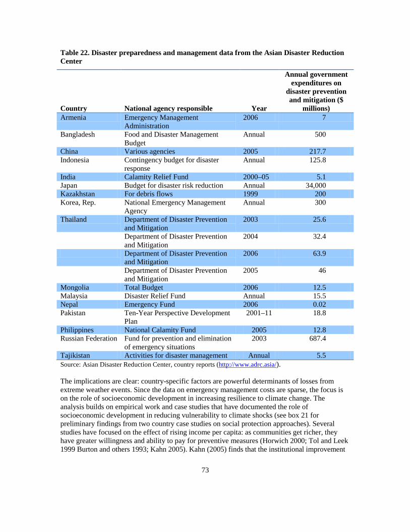
73

Table 22. Disaster preparedness and management data from the Asian Disaster Reduction Center

Country National agency responsible Year

Annual government expenditures on

disaster prevention and mitigation ($

millions) Armenia Emergency Management

Administration 2006 7

Bangladesh Food and Disaster Management Budget

Annual 500

China Various agencies 2005 217.7 Indonesia Contingency budget for disaster

response Annual 125.8

India Calamity Relief Fund 2000–05 5.1 Japan Budget for disaster risk reduction Annual 34,000 Kazakhstan For debris flows 1999 200 Korea, Rep. National Emergency Management

Agency Annual 300

Thailand Department of Disaster Prevention and Mitigation

2003 25.6

Department of Disaster Prevention and Mitigation

2004 32.4


2006 63.9


2005 46

Mongolia Total Budget 2006 12.5 Malaysia Disaster Relief Fund Annual 15.5 Nepal Emergency Fund 2006 0.02 Pakistan Ten-Year Perspective Development

Plan 2001–11 18.8

Philippines National Calamity Fund 2005 12.8 Russian Federation Fund for prevention and elimination

of emergency situations 2003 687.4

Tajikistan Activities for disaster management Annual 5.5 Source: Asian Disaster Reduction Center, country reports (http://www.adrc.asia/). The implications are clear: country-specific factors are powerful determinants of losses from extreme weather events. Since the data on emergency management costs are sparse, the focus is on the role of socioeconomic development in increasing resilience to climate change. The analysis builds on empirical work and case studies that have documented the role of socioeconomic development in reducing vulnerability to climate shocks (see box 21 for preliminary findings from two country case studies on social protection approaches). Several studies have focused on the effect of rising income per capita: as communities get richer, they have greater willingness and ability to pay for preventive measures (Horwich 2000; Tol and Leek 1999 Burton and others 1993; Kahn 2005). Kahn (2005) finds that the institutional improvement

http://www.adrc.asia/�

74

that accompanies economic development is also important, through enhanced public sector capability to organize disaster prevention and relief. Box 21. The importance of social protection measures Preliminary findings from the country case studies suggest that social safety nets and other social protection approaches are widely assigned high priority among measures to support pro-poor adaptation to climate change. Participants in scenario development workshops in Bangladesh named extension of citizenship rights to urban slum dwellers (as well as improved coverage of basic services) as key elements of their future vision. Preferred social protection interventions include both protective measures (safety nets, cash transfers) and productive measures (livelihoods, asset protection, attention to natural resources and agriculture). Safety net programs, when designed to address climate hazards, should include investments in risk preparedness and response systems, with attention to gender issues in disaster mitigation. And they should include investments in the construction of community-level physical assets, such as water storage and land management systems. Harmonization and coordination among actors involved in disaster risk management, social protection, and longer term development are considered important. Both the Productive Safety Net Program (Ethiopia) and National Rural Employment Guarantee Act (NREGA) in India (see box 23), for example, have elements that can be adapted to address climate risks. NREGA, in particular, has been shown to reduce distress migration in drought-affected sample villages by half. Other work focuses on political and human development. Albala-Bertrand (1993) identifies political marginalization as a source of vulnerability to natural disasters. Toya and Skidmore (2005) find a significant role for education in reducing vulnerability, through better choices in areas ranging from safe construction practices to assessment of potential risks. Recently, Oxfam International (2007, p. 1), drawing on extensive evidence from South Asia, highlights the particular vulnerability of women, who often suffer greater losses than men in natural disasters:

Nature does not dictate that poor people, or women, should be the first to die. Cyclones do not hand-pick their victims. Yet, history consistently shows that vulnerable groups end up suffering from such events disproportionately … In the 1991 Bangladesh cyclone, for example, four times more women died than men … Disasters are therefore an issue of unsustainable and unequal development at all levels ….

A logical inference from these studies is that empowering women through improved education is critical for reducing household vulnerability to weather-related disasters. This would also be consistent with the extensive literature on the powerful effect of female education on community-level social capital and general welfare measures such as life expectancy (World Bank 2001). Accordingly, the estimate of adaptation costs highlights the importance of female education and empowerment in reducing risks of weather-related loss. The cost analysis consider two key issues: How many additional young women would have to be educated to neutralize the increased vulnerability to extreme weather events resulting from climate changes? And how much would it cost (see box 22 for methodology)?

75

Box 22. Extreme weather events methodology

To address the question of how much it would cost to reduce household vulnerability to weather-related disasters by empowering women through improved education, a model of weather-related impact risk is estimated using panel data for 1960–2002. Use of panel data allows for clearer interpretation of results, because it absorbs many sources of potentially misleading cross-sectional correlation into estimated country effects. The need for lengthy time series limits the estimation variables to a sparse set, however. The study employs fixed effects estimation of risk equations that link losses from floods and droughts to three determinants: weather events that increase potential losses, income per capita, and female education. Separate equations are estimated for the risk of death from a flood, the risk of being affected by a flood, and the risk of being affected by a drought (the data are too sparse to support estimation for death from droughts). As in the other sector analyses, the study combines estimated risk equations with projections of economic growth, population growth, and changes in primary and secondary schooling. The same three scenarios are developed: a baseline with socioeconomic development but without climate change, and two scenarios with the same baseline development path but with alternative weather paths—a wet (NCAR) and a dry (CSIRO) scenario. For each scenario, the associated changes in the risks of death from floods and being affected by floods or droughts are calculated. Then, using the worst-case risk, the increase in female schooling that would neutralize this additional risk is calculated. The results are multiplied by expenditures per student to estimate the total education investment required to neutralize the additional weather risk posed by climate change. The approach here is conservative in that it is unlikely to underestimate the required investment and even imparts a strong upward bias. First, the cost assessment is based on general preparedness through increased education, rather than more narrowly targeted investment in emergency preparedness. Second, cost calculations are based on worst-case risk scenarios, which require the greatest increase in schooling to neutralize. (Extreme wet and dry scenarios are both worst-case scenarios for extreme weather, because they generate the greatest number of floods and droughts.) Third, only projected increases in vulnerability are included, not decreases. (An alternative would be a net impact analysis for a wet climate scenario that subtracts lower expected losses from drought from higher expected losses from flooding.) Finally, the results for the two model scenarios are not averaged, which would neutralize their extreme signals. This approach offers considerable co-benefits because female education has a much broader sphere of potential influence than as a direct investment in emergency preparedness. As the development literature has shown for many years, educating young women is a major determinant of sustainable development. A disaster prevention approach that focuses on investment in female education therefore has a broader expected social rate of return that justifies the exercise, even if the expected benefits from reduced disaster vulnerability are overstated (though more likely the opposite is true). Variations in projected climate, socioeconomic, and demographic variables produce wide disparities in outcomes for required female schooling and associated costs by 2050 (table 23), even among countries in the same region. At the country and regional levels, neither climate

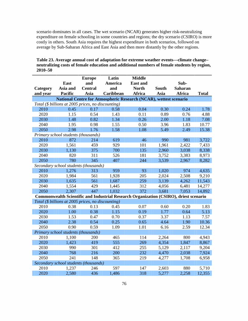
76

scenario dominates in all cases. The wet scenario (NCAR) generates higher risk-neutralizing expenditure on female schooling in some countries and regions; the dry scenario (CSIRO) is more costly in others. South Asia requires the highest expenditure in both scenarios, followed on average by Sub-Saharan Africa and East Asia and then more distantly by the other regions.

Table 23. Average annual cost of adaptation for extreme weather events—climate change–neutralizing costs of female education and additional numbers of female students by region, 2010–50

Category and year


Europe and

Central Asia

Latin America

and Caribbean

Middle East and

North Africa

South Asia


National Centre for Atmospheric Research (NCAR), wettest scenario Total ($ billions at 2005 prices, no discounting)

2010 0.45 0.17 0.58 0.04 0.30 0.24 1.78 2020 1.15 0.54 1.43 0.11 0.89 0.76 4.88 2030 1.48 0.82 1.34 0.26 2.00 1.18 7.08 2040 1.95 0.98 1.55 0.50 3.96 1.83 10.77 2050 2.98 1.76 1.58 1.08 5.49 2.49 15.38

Primary school students (thousands) 2010 872 214 619 46 990 981 3,722 2020 1,561 459 929 101 1,961 2,422 7,433 2030 1,130 375 700 135 2,960 3,038 8,338 2040 820 311 526 181 3,752 3,383 8,973 2050 780 345 407 244 3,539 2,967 8,282

Secondary school students (thousands) 2010 1,276 313 959 93 1,020 974 4,635 2020 1,984 561 1,928 205 2,024 2,508 9,210 2030 1,635 561 1,687 259 3,139 4,262 11,543 2040 1,554 429 1,445 312 4,056 6,481 14,277 2050 2,307 447 1,032 372 3,681 7,053 14,892

Commonwealth Scientific and Industrial Research Organization (CSIRO), driest scenario Total ($ billions at 2005 prices, no discounting)

2010 0.38 0.13 0.45 0.07 0.60 0.20 1.83 2020 1.00 0.38 1.15 0.19 1.77 0.64 5.13 2030 1.53 0.47 0.70 0.37 3.37 1.13 7.57 2040 2.38 0.54 0.25 0.65 4.64 1.90 10.36 2050 0.90 0.59 1.09 1.01 6.16 2.59 12.34

Primary school students (thousands) 2010 1,100 200 465 114 2,264 800 4,943 2020 1,423 419 555 269 4,354 1,847 8,867 2030 990 301 412 255 5,129 2,117 9,204 2040 768 216 200 232 4,470 2,038 7,924 2050 241 148 365 219 4,277 1,708 6,958

Secondary school students (thousands) 2010 1,237 246 597 147 2,603 880 5,710 2020 2,580 436 1,486 318 5,277 2,258 12,355

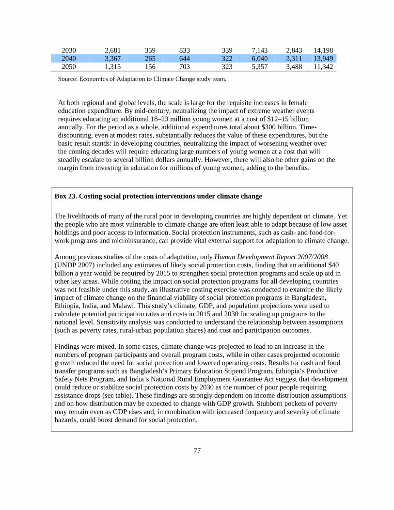
77

2030 2,681 359 833 339 7,143 2,843 14,198 2040 3,367 265 644 322 6,040 3,311 13,949 2050 1,315 156 703 323 5,357 3,488 11,342


At both regional and global levels, the scale is large for the requisite increases in female education expenditure. By mid-century, neutralizing the impact of extreme weather events requires educating an additional 18–23 million young women at a cost of $12–15 billion annually. For the period as a whole, additional expenditures total about $300 billion. Time-discounting, even at modest rates, substantially reduces the value of these expenditures, but the basic result stands: in developing countries, neutralizing the impact of worsening weather over the coming decades will require educating large numbers of young women at a cost that will steadily escalate to several billion dollars annually. However, there will also be other gains on the margin from investing in education for millions of young women, adding to the benefits.

Box 23. Costing social protection interventions under climate change

The livelihoods of many of the rural poor in developing countries are highly dependent on climate. Yet the people who are most vulnerable to climate change are often least able to adapt because of low asset holdings and poor access to information. Social protection instruments, such as cash- and food-for-work programs and microinsurance, can provide vital external support for adaptation to climate change. Among previous studies of the costs of adaptation, only Human Development Report 2007/2008 (UNDP 2007) included any estimates of likely social protection costs, finding that an additional $40 billion a year would be required by 2015 to strengthen social protection programs and scale up aid in other key areas. While costing the impact on social protection programs for all developing countries was not feasible under this study, an illustrative costing exercise was conducted to examine the likely impact of climate change on the financial viability of social protection programs in Bangladesh, Ethiopia, India, and Malawi. This study’s climate, GDP, and population projections were used to calculate potential participation rates and costs in 2015 and 2030 for scaling up programs to the national level. Sensitivity analysis was conducted to understand the relationship between assumptions (such as poverty rates, rural-urban population shares) and cost and participation outcomes. Findings were mixed. In some cases, climate change was projected to lead to an increase in the numbers of program participants and overall program costs, while in other cases projected economic growth reduced the need for social protection and lowered operating costs. Results for cash and food transfer programs such as Bangladesh’s Primary Education Stipend Program, Ethiopia’s Productive Safety Nets Program, and India’s National Rural Employment Guarantee Act suggest that development could reduce or stabilize social protection costs by 2030 as the number of poor people requiring assistance drops (see table). These findings are strongly dependent on income distribution assumptions and on how distribution may be expected to change with GDP growth. Stubborn pockets of poverty may remain even as GDP rises and, in combination with increased frequency and severity of climate hazards, could boost demand for social protection.

78

Projected impact of climate change on illustrative social protection programs

Country and program

Impacts with EACC growth projections and significant reductions in rural poverty

Impacts with EACC growth projections and significant increases in rural poverty

Ethiopia, Productive Safety Nets Program

While significant resources are needed to provide social protection in 2015, total beneficiaries and costs are only slightly higher in 2030

Numbers of beneficiaries and total costs of the program nearly double between 2015 and 2030 because of lower agricultural productivity and greater incidence of droughts and floods (Diao and others 2005)

India, National Rural Employment Guarantee Act

For the most part, income growth outpaces population growth, resulting in smaller numbers of rural poor and lower program costs in 2015 and 2030 than in 2007

Numbers of rural poor and costs of the program increase between 2007 and 2015 but decline subsequently

Source: Economics of Adaptation to Climate Change study team. Analysis of selected microinsurance programs (the BASIX index-based microinsurance program in Andhra Pradesh, India, and Malawi’s rainfall-based index insurance product for maize farmers) suggests that the programs could become insolvent if projected increases in the frequency and severity of extreme weather events materialize. This would occur because of strong covariate risk and increased likelihood of extremes of droughts and flooding (Hochrainer and Linnerooth-Bayer 2009). Any long-run change in the frequency or severity of such hazards means that the risks can no longer be priced on the basis of the historical record, thus likely precluding an insurance-based solution. Social protection programs play a vital role in helping the poorest and most vulnerable to climate change deal with its consequences. Yet the projected increase in intensity of floods and droughts is likely to adversely affect the financial viability of many such programs, at least in the near term. Further research to understand the full implications of climate change on social protection should be a priority.

C onsolidated r esults

Overall, the study estimates the costs of adaptation to climate change in developing countries at $75–100 billion a year over 2010–50, depending on the aggregation rule used (see section 3), and the climate scenario—National Centre for Atmospheric Research (NCAR) or Commonwealth Scientific and Industrial Research Organization (CSIRO) (table 24). The costs of adaptation are roughly $80– $90 billion for the X-sum aggregation methods.

79

Table 24. Total annual costs of adaptation for all sectors, by region, 2010–50 ($ billions at 2005 prices, no discounting)

Cost aggregation type

East Asia and

Pacific

Europe and

Central Asia

Latin America

and Caribbean

Middle East and

North Africa

South Asia


National Centre for Atmospheric Research (NCAR), wettest scenario Gross sum 28.7 10.5 22.5 4.1 17.1 18.9 101.8 X-sum 25.0 9.4 21.5 3.0 12.6 18.1 89.6 Net sum 25.0 9.3 21.5 3.0 12.6 18.1 89.5

Commonwealth Scientific and Industrial Research Organization (CSIRO), driest scenario Gross sum 21.8 6.5 18.8 3.7 19.4 18.1 88.3 X-sum 19.6 5.6 16.9 3.0 15.6 16.9 77.6 Net sum 19.5 5.2 16.8 2.9 15.5 16.9 76.8

Note: Gross sum is the aggregate cost for all positive costs incurred by countries for a particular sector, ignoring all country and sector combinations resulting in negative costs. Net sum includes both positive and negative costs. X-sum sets all costs for a given country at zero if the net sum for the country is negative.


The costs are high, at approximately equal to current official development assistance (OECD 2008). The highest costs are in East Asia and Pacific, followed closely by Latin America and the Caribbean and Sub-Saharan Africa. The dry scenario, CSIRO, requires lower adaptation costs overall and in all regions but South Asia. The lower total costs under CSIRO reflect lower costs for infrastructure, health, and extreme weather events than under NCAR, more than compensating for higher costs for water supply and flood protection and agriculture. Total adaptation costs calculated by the gross sum method average $10 billion a year more than by the other two methods (the insignificant difference between the X-sum and net sum figures is largely coincidence). Countries that appear to benefit from climate change in the water supply and flood protection sector, especially in East Asia and Pacific and South Asia, drive this difference. Not surprising, both climate scenarios show costs increasing over time (table 25). Under the NCAR scenario, annual adaptation costs are $73 billion during 2010–19, rising 45 percent over the next 30 years to reach $106 billion in 2040–49. Under the CSIRO scenario, growth is more rapid, through from a lower base, rising 67 percent over the entire period, from $57 billion a year in 2010–19 to $95 billion by 2040–49. Under the NCAR scenario, there is little variation in costs over the 40-year period in East Asia and Pacific and Latin America and the Caribbean. Costs grow most rapidly in the Middle East and North Africa, rising 1.6 times over the four decades. A key finding is that adaptation costs decline as a percentage of GDP over time, suggesting that countries become less vulnerable to climate change as their economies grow (table 26). There are considerable regional variations, however. Adaptation costs as a percentage of GDP are highest in Sub-Saharan Africa, in large part because GDP is lower in the region. Percentages remain stable in Europe and Central Asia and the Middle East and North Africa and fall sharply in all other regions.

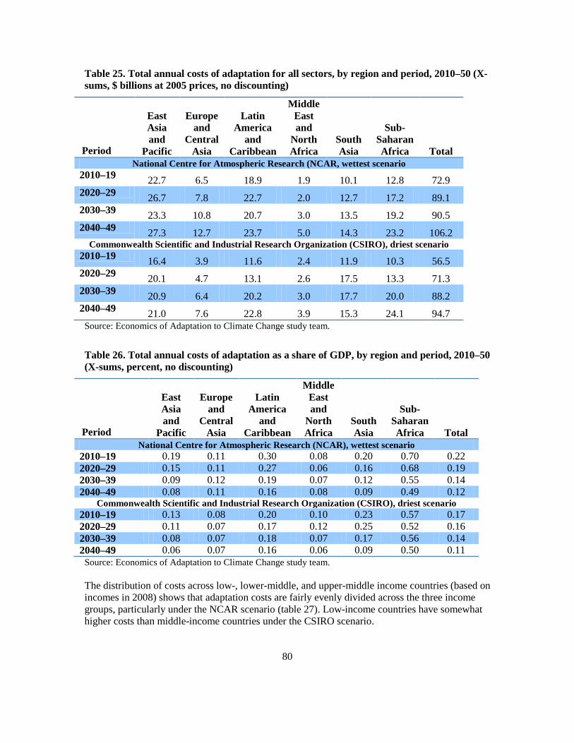
80

Table 25. Total annual costs of adaptation for all sectors, by region and period, 2010–50 (X-sums, $ billions at 2005 prices, no discounting)

Period

East Asia and

Pacific

Europe and

Central Asia

Latin America

and Caribbean

Middle East and

North Africa

South Asia


National Centre for Atmospheric Research (NCAR, wettest scenario 2010–19 22.7 6.5 18.9 1.9 10.1 12.8 72.9 2020–29 26.7 7.8 22.7 2.0 12.7 17.2 89.1 2030–39 23.3 10.8 20.7 3.0 13.5 19.2 90.5 2040–49 27.3 12.7 23.7 5.0 14.3 23.2 106.2

Commonwealth Scientific and Industrial Research Organization (CSIRO), driest scenario 2010–19 16.4 3.9 11.6 2.4 11.9 10.3 56.5 2020–29 20.1 4.7 13.1 2.6 17.5 13.3 71.3 2030–39 20.9 6.4 20.2 3.0 17.7 20.0 88.2 2040–49 21.0 7.6 22.8 3.9 15.3 24.1 94.7


Table 26. Total annual costs of adaptation as a share of GDP, by region and period, 2010–50 (X-sums, percent, no discounting)

Period

East Asia and

Pacific

Europe and

Central Asia

Latin America

and Caribbean

Middle East and

North Africa

South Asia


National Centre for Atmospheric Research (NCAR), wettest scenario 2010–19 0.19 0.11 0.30 0.08 0.20 0.70 0.22 2020–29 0.15 0.11 0.27 0.06 0.16 0.68 0.19 2030–39 0.09 0.12 0.19 0.07 0.12 0.55 0.14 2040–49 0.08 0.11 0.16 0.08 0.09 0.49 0.12

Commonwealth Scientific and Industrial Research Organization (CSIRO), driest scenario 2010–19 0.13 0.08 0.20 0.10 0.23 0.57 0.17 2020–29 0.11 0.07 0.17 0.12 0.25 0.52 0.16 2030–39 0.08 0.07 0.18 0.07 0.17 0.56 0.14 2040–49 0.06 0.07 0.16 0.06 0.09 0.50 0.11

Source: Economics of Adaptation to Climate Change study team. The distribution of costs across low-, lower-middle, and upper-middle income countries (based on incomes in 2008) shows that adaptation costs are fairly evenly divided across the three income groups, particularly under the NCAR scenario (table 27). Low-income countries have somewhat higher costs than middle-income countries under the CSIRO scenario.

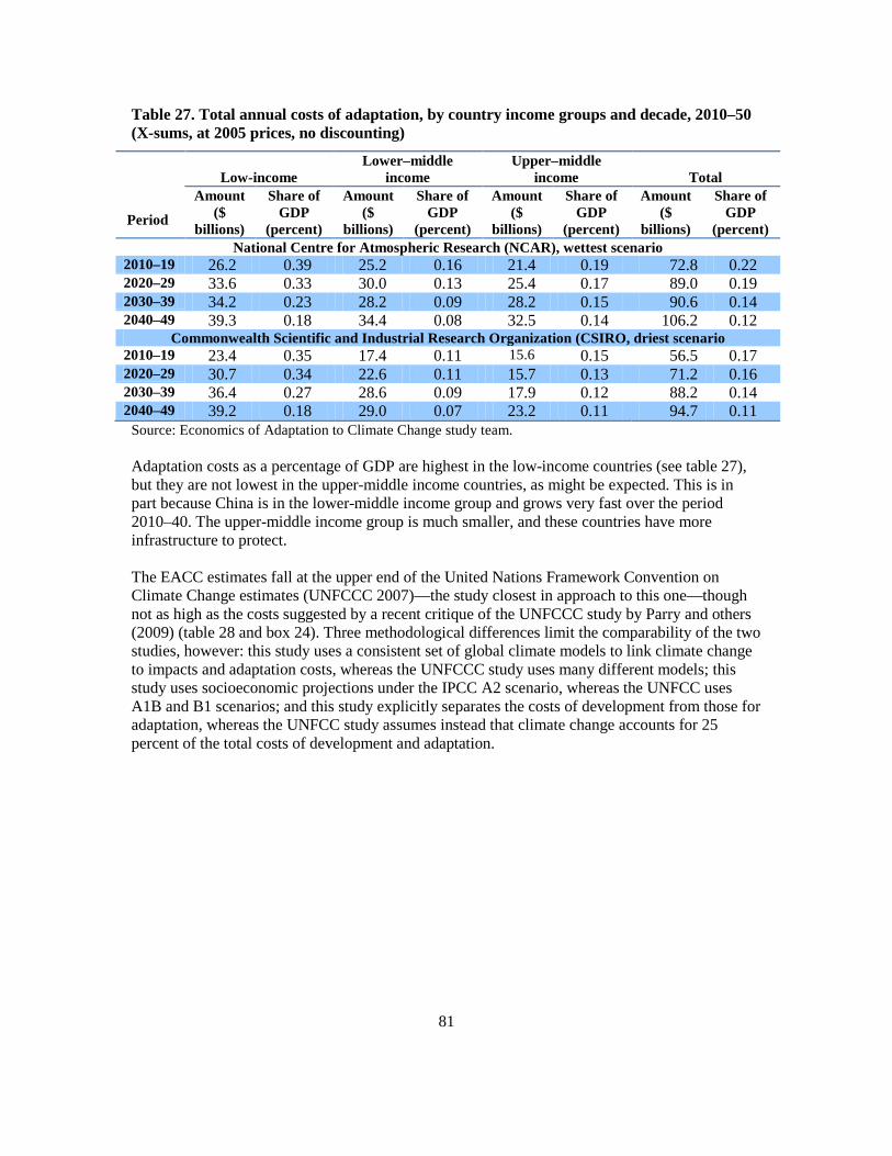
81

Table 27. Total annual costs of adaptation, by country income groups and decade, 2010–50 (X-sums, at 2005 prices, no discounting)

Period

Low-income Lower–middle

income Upper–middle

income Total Amount

($ billions)

Share of GDP

(percent)

Amount ($

billions)

Share of GDP

(percent)

Amount ($

billions)

Share of GDP

(percent)

Amount ($

billions)

Share of GDP

(percent) National Centre for Atmospheric Research (NCAR), wettest scenario

2010–19 26.2 0.39 25.2 0.16 21.4 0.19 72.8 0.22 2020–29 33.6 0.33 30.0 0.13 25.4 0.17 89.0 0.19 2030–39 34.2 0.23 28.2 0.09 28.2 0.15 90.6 0.14 2040–49 39.3 0.18 34.4 0.08 32.5 0.14 106.2 0.12

Commonwealth Scientific and Industrial Research Organization (CSIRO, driest scenario 2010–19 23.4 0.35 17.4 0.11 15.6 0.15 56.5 0.17 2020–29 30.7 0.34 22.6 0.11 15.7 0.13 71.2 0.16 2030–39 36.4 0.27 28.6 0.09 17.9 0.12 88.2 0.14 2040–49 39.2 0.18 29.0 0.07 23.2 0.11 94.7 0.11

Source: Economics of Adaptation to Climate Change study team. Adaptation costs as a percentage of GDP are highest in the low-income countries (see table 27), but they are not lowest in the upper-middle income countries, as might be expected. This is in part because China is in the lower-middle income group and grows very fast over the period 2010–40. The upper-middle income group is much smaller, and these countries have more infrastructure to protect. The EACC estimates fall at the upper end of the United Nations Framework Convention on Climate Change estimates (UNFCCC 2007)—the study closest in approach to this one—though not as high as the costs suggested by a recent critique of the UNFCCC study by Parry and others (2009) (table 28 and box 24). Three methodological differences limit the comparability of the two studies, however: this study uses a consistent set of global climate models to link climate change to impacts and adaptation costs, whereas the UNFCCC study uses many different models; this study uses socioeconomic projections under the IPCC A2 scenario, whereas the UNFCC uses A1B and B1 scenarios; and this study explicitly separates the costs of development from those for adaptation, whereas the UNFCC study assumes instead that climate change accounts for 25 percent of the total costs of development and adaptation.

82

Table 28. Comparison of adaptation cost estimates by the United Nations Framework Convention on Climate Change, Parry and others, and the Economics of Adaptation to Climate Change study, by sector ($ billions)

Sector

United Nations

Framework Convention on Climate

Change (2007)

Parry and others (2009)

Economics of Adaptation to Climate Change study (in 2005 prices, no

discounting)


Research (NCAR), wettest

scenario

Commonwealth Scientific and

Industrial Research Climate (CSIRO), driest

scenario Infrastructure 2-41 18–104 29.5 13.5 Coastal zones 5 15 30.1 29.6 Water supply and flood protection

9 >9 13.7 19.2

Agriculture,a forestry, fisheries

7 >7 7.6 7.3

Human health 5 >5 2 1.6 Extreme weather events — — 6.7 6.5 Total 28–67 — 89.6 77.7 a. The baseline provision of rural roads up to 2050 used to estimate costs of adaptation is adjusted to account for the additional length of rural roads consistent with the baseline projections for road investment. This adjustment reduces the investment in rural roads included in the cost of adaptation for agriculture by about 80–85 percent for the two climate scenarios. The adjustment for these overlaps amounts to $2.0–2.2 billion a year averaged over the full period.

Source: UNFCCC (2007); Parry and others (2009), and Economics of Adaptation to Climate Change study team.

Box 24. Critique of the United Nations Framework Convention on Climate Change estimates by Parry and others

A recent critique of the United Nations Framework Convention on Climate Change (UNFCCC 2007) estimates of adaptation costs by Parry and others (2009) argues that the estimates may be too low because some sectors (ecosystems, energy, manufacturing, retailing, and tourism) are not covered, some sectors are not fully covered, estimates for climate-proofing infrastructure stocks do not account for the need to climate proof the adaptation deficit, and residual damages (impacts remaining after adaptation) are not counted. Agriculture, forestry, and fisheries. Parry and others (2009) suggest that UNFCCC estimates in these sectors are low because they underestimate costs to maintain irrigation capacity under climate change and do not account for residual damage (a study of the wheat crop in Australia found residual damage costs to be about 20 percent of total damages). The EACC estimate for these sectors is even lower than the UNFCCC estimate. Water supply. Parry and others (2009) argue that the UNFCCC estimate is an underestimate because it does not account for the costs of managing increased flood risk, maintaining water

83

quality standards, and supporting in-stream economic and environmental use or consider residual damages and operating costs. Parry and others also critique the UNFCCC study for failing to use hydrologic models to estimate changes in reservoir capacity. The EACC analysis of water supply and flood protection avoids most of these shortfalls and is, consequently, higher. Infrastructure. Parry and others argue that low- and middle-income countries have a large infrastructure deficit, and that the costs of climate-proofing this additional infrastructure must be included in the adaptation costs. Parry and others estimate the additional costs at $16–63 billion a year. The bulk of the estimates for the infrastructure sector in the EACC study are for observed levels of infrastructure. But even after closing the adaptation deficit by allowing for an optimal level of infrastructure the EACC estimates remain much lower, at $30 billion under the wetter NCAR scenario and $14 billion under the drier CSIRO scenario.

Ecosystem services. The UNFCCC estimates do not include ecosystem services. Costs for ecosystem services have been defined by Parry and others as the costs of expanding and protecting terrestrial protected area networks so that they represent 10 percent of each country’s land area, costs of marine protected areas covering 30 percent of total area of the seas, and costs of biodiversity conservation in a wider matrix of landscapes. This approach to costing adaptation for ecosystems services would suggest that the development deficit should be part of the adaptation costs, an approach not used by the EACC. Instead, in the EACC estimates, some ecosystem services are covered in other sectors.

The major difference between the estimates is the sixfold increase the cost of coastal zone management and defense under the EACC study. This difference reflects several improvements to the earlier UNFCCC estimates under the EACC study: better unit cost estimates, including maintenance costs, and inclusion of costs of port upgrading, and of risks from both sea-level rise and storm surges. Another difference is the higher costs of adaptation for water supply and flood protection under the EACC study, particularly for the drier climate scenario, CSIRO. This difference is explained in part by the inclusion of riverine flood protection costs under the EACC study. Also pushing up the EACC study estimate is the study’s comprehensive sector coverage, especially inclusion of the cost of adaptation to extreme weather events. On the other hand, adaptation costs in the human health sector are lower in the EACC study than in the UNFCCC study, in part because inclusion of the development baseline reduces the number of additional cases of malaria, and thereby adaptation costs, by some 50 percent by 2030 under the EACC study. Part of the difference is also explained by differences in sectoral coverage: while the UNFCCC study includes malnutrition under the health sector, the EACC study includes it under the agriculture sector. The infrastructure costs of adaptation in the EACC study fall sin the middle of the UNFCCC range because of two contrary forces. Pushing up the EACC estimate is the more detailed coverage of infrastructure. Previous studies estimated adaptation costs as the costs of climate-proofing new investment flows and did not differentiate risks or costs by type of infrastructure.

84

The EACC study extended this work to estimate costs by types of infrastructure services—energy, transport, water and sanitation, communications, and urban and social infrastructure. Pushing down the EACC study estimate are measurements of adaptation against a consistently projected development baseline and use of a smaller multiplier on baseline investments than in the previous literature, based on detailed analysis of climate proofing, including adjustments to design standards and maintenance costs. On average, the EACC study derives a multiplier of 1.6 percent while the previous literature applied multipliers as high as 8 percent. The UNFCCC study uses an upper bound of 0.6 percent.

Sensitivity analysis While climate scientists can speak with conviction about general global trends of climate change, there is a high degree of uncertainty about the extent and timing of the impact of climate change on individual economies and socioeconomic groups, how these groups will respond, what the benefits and costs will be planned adaptation measures, and how these factors will change over time. Three broad types of uncertainty that affect the estimation of the costs of adaptation presented in this report were assessed using sensitivity analysis: • Uncertainty about future climate outcomes. How might the estimates have differed had

alternative global climate models been used to project climate conditions? • Uncertainty about the development baseline. What if a different future were to evolve? • Uncertainty about the structure of the models and the parameters used. In addition, it is possible that actual patterns of climate change might affect the aggregate rate and distribution of economic growth and how countries respond to climate change through technological advances or the design of future economic policies. These issues are outside the scope of this study.

Uncer tainty about climate pr ojections

The analysis of adaptation costs is based on two climate scenarios, the wetter NCAR and the drier CSIRO, in an attempt to capture some of the uncertainty about future climate conditions. But these are only two global climate models among all the IPCC AR4 models archived at phase 3 of the Coupled Model Intercomparison Project (CMIP3) for the A2 scenario. The scenarios are the wettest and driest of the climate models that provide the minimum and maximum temperatures required for modeling the agriculture and infrastructure sectors. While providing a range of estimates, the two scenarios alone do not give a sense of the impact of uncertainty in climate projections on cost estimates. An analysis that draws on all the IPCC AR4 models archived at CMIP3 for the A2 scenario for all sectors was beyond the time and resource constraints of this study. A limited Monte Carlo analysis was conducted for the infrastructure sector and provides some sense of the potential impact of uncertainty about climate outcomes. The analysis finds that a small number of countries face enormous variability in the costs of adapting to climate change given the uncertainty about the extent and nature of climate change. Managing this risk will need to be a key policy concern in these countries.

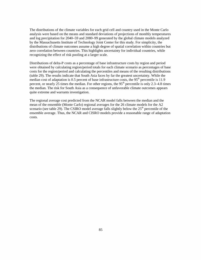
http://www-pcmdi.llnl.gov/projects/cmip/index.php�

85

The distributions of the climate variables for each grid cell and country used in the Monte Carlo analysis were based on the means and standard deviations of projections of monthly temperatures and log precipitation for 2040–59 and 2080–99 generated by the global climate models analyzed by the Massachusetts Institute of Technology Joint Center for this study. For simplicity, the distributions of climate outcomes assume a high degree of spatial correlation within countries but zero correlation between countries. This highlights uncertainty for individual countries, while recognizing the effect of risk pooling at a larger scale. Distributions of delta-P costs as a percentage of base infrastructure costs by region and period were obtained by calculating region/period totals for each climate scenario as percentages of base costs for the region/period and calculating the percentiles and means of the resulting distributions (table 29). The results indicate that South Asia faces by far the greatest uncertainty. While the median cost of adaptation is 0.5 percent of base infrastructure costs, the 95th percentile is 11.9 percent, or nearly 25 times the median. For other regions, the 95th percentile is only 2.3–4.8 times the median. The risk for South Asia as a consequence of unfavorable climate outcomes appears quite extreme and warrants investigation. The regional average cost predicted from the NCAR model falls between the median and the mean of the ensemble (Monte Carlo) regional averages for the 26 climate models for the A2 scenario (see table 29). The CSIRO model average falls slightly below the 25th percentile of the ensemble average. Thus, the NCAR and CISRO models provide a reasonable range of adaptation costs.

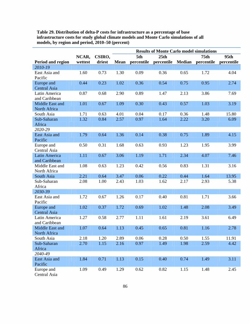
86

Table 29. Distribution of delta-P costs for infrastructure as a percentage of base infrastructure costs for study global climate models and Monte Carlo simulations of all models, by region and period, 2010–50 (percent)

Period and region NCAR, wettest

CSIRO, driest

Results of Monte Carlo model simulations

Mean 5th

percentile 25th

percentile Median 75th

percentile 95th

percentile 2010-19 East Asia and Pacific

1.60 0.73 1.30 0.09 0.36 0.65 1.72 4.04

Europe and Central Asia

0.44 0.23 1.02 0.36 0.54 0.75 0.95 2.74


0.87 0.68 2.90 0.89 1.47 2.13 3.86 7.69


1.01 0.67 1.09 0.30 0.43 0.57 1.03 3.19

South Asia 1.71 0.63 4.01 0.04 0.17 0.36 1.48 15.80 Sub-Saharan Africa

1.32 0.84 2.57 0.97 1.64 2.22 3.20 6.09

2020-29 East Asia and Pacific

1.79 0.64 1.36 0.14 0.38 0.75 1.89 4.15


0.50 0.31 1.68 0.63 0.93 1.23 1.95 3.99


1.11 0.67 3.06 1.19 1.71 2.34 4.07 7.46


1.08 0.63 1.23 0.42 0.56 0.83 1.31 3.16


2.08 1.00 2.43 1.03 1.62 2.17 2.93 5.38


1.72 0.67 1.26 0.17 0.40 0.81 1.71 3.66


1.02 0.37 1.72 0.69 1.02 1.48 2.08 3.49


1.27 0.58 2.77 1.11 1.61 2.19 3.61 6.49


1.07 0.64 1.13 0.45 0.65 0.81 1.16 2.78


2.70 1.15 2.16 0.97 1.49 1.98 2.59 4.42


1.84 0.71 1.13 0.15 0.40 0.74 1.49 3.11


1.09 0.49 1.29 0.62 0.82 1.15 1.48 2.45

87


1.49 0.58 2.32 0.95 1.36 1.88 2.96 5.27


1.04 0.81 0.93 0.45 0.59 0.70 0.95 2.08


3.23 1.38 1.86 0.89 1.34 1.72 2.21 3.59

Full period East Asia and Pacific

1.76 0.69 1.23 0.16 0.41 0.75 1.65 3.57


0.80 0.37 1.45 0.61 0.89 1.21 1.64 3.01


1.24 0.61 2.68 1.05 1.53 2.10 3.51 6.44


1.05 0.70 1.06 0.42 0.58 0.74 1.09 2.63


2.57 1.15 2.14 0.96 1.48 1.93 2.56 4.43

Period mean 1.58 0.79 1.91 0.54 0.86 1.21 1.99 5.34 Note: The analysis draws on all the IPCC AR4 models archived at phase 3 of the Coupled Model Intercomparison Project (CMIP3) for the A2 scenario. Delta-P cost is the adaptation cost computed as the additional cost of constructing, operating, and maintaining baseline levels of infrastructure services under the new climate conditions projected by the two global climate models. Source: Economics of Adaptation to Climate Change study team.

Uncer tainty about the development baseline

A key contribution of this study is its attempt to separate the costs of adaptation from those of development by defining a development baseline. But here, too, the study assumes just one future development path. How would the costs of adaptation change with a different development path? The basic elements of the development baseline are growth in population, GDP per capita, and urbanization, which drive the demand for food; investment in infrastructure; benefits of protecting coastal zones; and so on and thus determine the costs of adaptation. One aspect of uncertainty is that the development baseline grows exponentially over time. Alternative assumptions about population and economic growth have only slight impact on estimates of the cost of adaptation in 2010–19, so the margins of error associated with the development baseline are not very important in the immediate future. But these margins of error grow over time, so the discussion focuses on estimates of the costs of adaptation for 2040–49, which rely on economic and population forecasts for 2050. The United Nations publishes alternative population projections that rely on different assumptions about the decline of fertility in developing countries. The variation in population forecasts for developing countries in 2050 is approximately +/–14 percent for the alternative fertility assumptions. The United Nation’s central projection has consistently been revised downward over the last two decades as fertility rates have fallen faster than anticipated. Thus, the plausible range of uncertainty might be +/–10 percent. The range of uncertainty for growth in GDP per capita is larger. The economic models used to generate the baseline GDP projection



88

have a range of –26 percent to +40 percent for global GDP in 2050 using the medium fertility population projection. The variation for developing countries is even larger—from –40 percent to +50 percent—so the range of variation in total GDP might be –45 percent to +75 percent, a huge margin of uncertainty. These errors are compounded by the confidence intervals of projections of demand as functions of population and GDP per capita. On this basis, it is very difficult to calculate potential margins of error in the estimates of the costs of adaptation. Sensitivity of adaptation cost estimates in agriculture was explored using a 10 percent increase in per capita GDP relative to the baseline projections and a 10 percent increase in population (table 30). Across all developing countries, a 10 percent increase in per capita GDP under the baseline results in a 1.4 percent overall decline in the number of malnourished children, with the greatest declines in East Asia and Pacific and the Middle East and North Africa of about 3.5 percent. A 10 percent increase in population growth has a much larger, and negative, effect on the number of malnourished children, which rises by about 8 percent, with the greatest increases in the Middle East and North Africa and Sub-Saharan Africa. Table 30. Percentage change in number of malnourished children with a 10 percent increase in GDP per capita and population growth, by region and climate scenario, 2010–50

Climate Scenario

South Asia


Europe and

Central Asia

Latin America

and Caribbean

Middle East and

North Africa


10 percent increase in GDP per capita NCAR, wettest scenario

–0.8 –3.5 –0.3 –0.2 –3.5 –1.7 –1.4

CSIRO, driest scenario

–0.8 –3.5 –0.3 –0.2 –3.6 –1.7 –1.4

10 percent increase in population NCAR, wettest scenario

5.2 5.9 5.0 5.7 10.0 11.9 7.9

CSIRO, driest scenario

5.2 6.0 5.1 5.7 10.2 11.9 7.9


A more robust sensitivity test considers how much the costs of adaptation increase or decrease as a percentage of GDP at higher and lower economic and population baselines. For most sectors and especially overall, the cost of adaptation as a share of GDP falls as GDP rises (see, for example, tables 26 and 27, which show that this effect is stronger than any increase in the impact of climate change over time). Three factors account for this relationship:

89

• Adaptation has large fixed costs that are substantially independent of future levels of GDP

and population, particularly for those protecting populated coastal zones. The analysis of coastal protection allows for residual damages, which increase with population and GDP per capita, but this is a small fraction of the total cost and is limited by the option of providing more extensive protection. Maintenance of existing infrastructure that is not adapted to changed climate conditions is also a fixed cost that diminishes over time.

• The income and population elasticities of demand for infrastructure, food, and water are well

below one, so that higher aggregate GDP does not translate into proportionately higher costs of investing in or operating fixed assets.

• The relationships between the development baseline and the costs of adapting to climate

change for health and extreme weather events operate to reduce the costs of adaptation as GDP per capita increases. Higher population could weaken their relationship somewhat, but the overall direction of change is a strong downward trend in the cost of adaptation.

In summary, uncertainty about the development baseline is not likely to have an important impact on the estimates of the costs of adaptation as a percentage of GDP for 2010–19; however, the impact increases over time. Under the NCAR scenario with the EACC development baseline projection, the overall cost of adaptation falls from 0.22 percent of developing world GDP in 2010–19 to 0.12 percent in 2040–49 (see table 26). With a range of uncertainty for aggregate GDP of –45 percent to +75 percent, trend projections indicate that the associated costs of adaptation would range from 0.16 percent of GDP in 2040–49 (low economic growth) to 0.09 percent of GDP in 2040–49 (high economic growth), with a central value of 0.12 percent.

M odel and par ameter uncer tainty

All sector analyses rely on large numbers of model assumptions and parameters that feed into the estimation of the cost of adaptation. Some examples: • Infrastructure. Dose-response relationships linking changes in climate variables to changes

in design standards and average costs of construction, changes in operating efficiency and costs under different ambient conditions, baseline construction and maintenance costs.

• Coastal zones. Unit costs of building dikes or undertaking beach nourishment, exposure of

coastal zones to flooding and permanent inundation, relationships between aggregate GDP and the decision to protect segments of coast.

• Water supply and flood protection. Runoff curves, the unit costs of building additional water

storage and river flood defenses, and the backstop cost of alternative ways of meeting demand for water.

• Agriculture. Elasticities of agricultural production to investments in research, irrigation

improvements, and rural roads; impact of changes in trade margins; substitution in demand between food products.

90

Some variables, such as unit costs, affect the estimates of adaptation costs in a linear manner, so that increasing one or more unit costs by 10 percent will increase the associated costs by the same percentage. However, almost all sectors include strongly nonlinear elements. For infrastructure, the costs of adaptation for many assets incorporate step functions so that, for example, the average cost of constructing and maintaining paved roads increases with each 3°C increase in maximum temperature or 100 millimeter increase in total precipitation. Such nonlinearities mean that it is difficult to estimate the sensitivity of adaptation costs to model and parameter uncertainty without detailed investigations using Monte Carlo or similar techniques. Such work was not feasible within the time and resources available for this study, and it remains a matter for further research. One additional form of model uncertainty was examined for the infrastructure sector. The analysis in section 5 is based on a definition of the development baseline that starts from current levels of infrastructure provision, rather than some higher level that includes an adjustment for the adaptation deficit. If it is assumed (as it was in section 5) that countries are currently allocating their resources efficiently, neither underinvesting nor overinvesting in infrastructure, there is no adaptation deficit and the development baseline can be based on current levels of infrastructure. If, however, it is assumed that countries should be investing more or less in infrastructure, and less or more in some other sector of the economy, then an adaptation deficit exists. This deficit is incorporated into the analysis by calculating adaptation costs for a higher level of infrastructure in each period. This deficit can only be approximated. One way is to compare countries of similar levels of income and select the one with the best performance in infrastructure investment as the most efficient. The development deficit is measured as the difference between actual levels of infrastructure and predicted levels derived from frontier regressions that fit the outer envelope of infrastructure stocks given the values of exogenous variables. These frontier regressions define the baseline projections used in calculating the costs of adaptation. The difference between the two approaches to defining the development baseline is that the baseline without the adaptation deficit starts with lower initial stocks of infrastructure but may imply greater investment in constructing new infrastructure in the future than the baseline with the adaptation deficit. On the other hand, the baseline with the adaptation deficit assumes a higher initial stock of infrastructure, which must be maintained and replaced over time, but it may imply lower investment in additions to the stock of infrastructure in future years. Depending on the relative costs of adaptation for existing stocks and new investments, either approach might yield higher total costs of adaptation. The costs of adaptation adjusted for the adaptation deficit are consistently higher than those derived from actual investment decisions, in total and in each decade to 2050 (table 31). Under the NCAR scenario and over the entire 40-year period, adaptation costs are 23 percent higher adjusting for the adaptation deficit than are those based on actual investment decisions. Under the CSIRO scenario, this difference rises to 26 percent. These higher costs arise because the extra costs of maintaining and replacing a larger initial stock of infrastructure outweigh the higher costs of construction for a larger investment program in later periods, even without discounting.

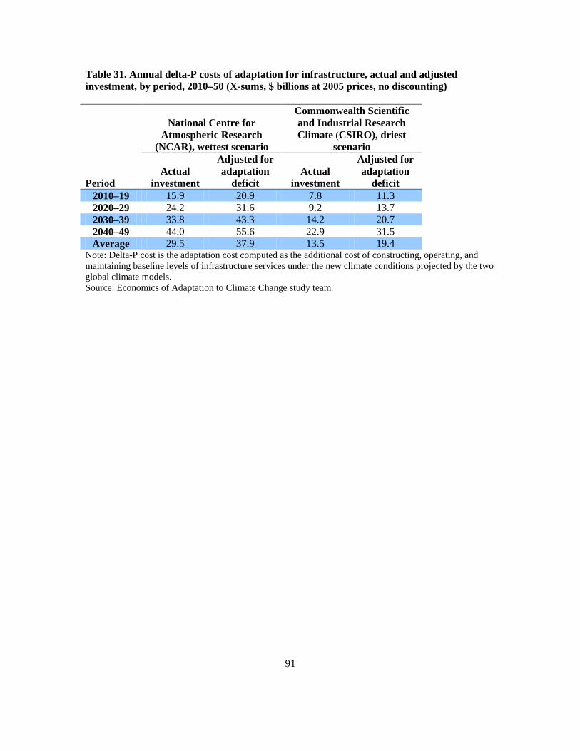
91

Table 31. Annual delta-P costs of adaptation for infrastructure, actual and adjusted investment, by period, 2010–50 (X-sums, $ billions at 2005 prices, no discounting)

Period

National Centre for Atmospheric Research


Commonwealth Scientific and Industrial Research Climate (CSIRO), driest

scenario

Actual investment

Adjusted for adaptation

deficit Actual

investment

Adjusted for adaptation

deficit 2010–19 15.9 20.9 7.8 11.3 2020–29 24.2 31.6 9.2 13.7 2030–39 33.8 43.3 14.2 20.7 2040–49 44.0 55.6 22.9 31.5 Average 29.5 37.9 13.5 19.4

Note: Delta-P cost is the adaptation cost computed as the additional cost of constructing, operating, and maintaining baseline levels of infrastructure services under the new climate conditions projected by the two global climate models. Source: Economics of Adaptation to Climate Change study team.

92

Section 6. K ey L essons

The sectoral estimates of adaptation costs presented in this report point to a number of lessons. A key lesson is that adaptation to a 2°C warmer world will be costly—and it will be even more costly if countries fail to take mitigation measures to avoid even greater warming and other climate change.

Development is imper ative… Development is adaptation and must remain a global imperative. Not only does development make economies less reliant on climate-sensitive sectors, such as agriculture, but by increasing levels of incomes, health, and education, it expands the capacity of households to adapt, and by improving institutional infrastructure, it enhances the ability of governments to assist.

Development dramatically reduces the numbers of people killed by floods and affected by floods and droughts, quite apart from the impact of climate change (figure 4). If development is held constant at 2000 levels, the number of people killed by floods increases over time under the NCAR (wettest) scenario and decrease under the CSIRO (driest) scenario. Allowing for development between 2000 and 2050 shows large reductions in the numbers of people killed under both scenarios. The findings are similar for the number of people affected by floods and droughts.

In the health sector analysis, allowing for development reduces the number of additional cases of malaria, and thereby adaptation costs, by more than half by 2030 and more than three-quarters by 2050.

The greater the baseline level of development in each period, the smaller is the impact of climate change and by the smaller are the costs of adaptation. Development must be inclusive, however, to have these effects. And development can also increase vulnerabilities: the more developed the country, the greater the value of infrastructure and personal property at risk from climate change and therefore greater the cost of climate-proofing such assets. However, these costs decrease with development as a percentage of GDP.

93

Figure 4. Development greatly lowers the umber of people killed by floods and affected by floods and droughts, 2000–50


…but not simply development as usual Adaptation will also require a different kind of development—breeding crops that are drought and flood tolerant, climate-proofing infrastructure to make it resilient to climate risks, reducing overcapacity in the fisheries industry, accounting for the inherent uncertainty in future climate projections in development planning.

Consider water supply. Adapting to changing conditions in water availability and demand has always been at the core of water management. Traditionally, though, water managers and users have relied on historical experience in planning. Water supply management has concentrated on meeting increasing water demand, and flood defense measures have assumed consistency in flood recurrence periods. These assumptions no longer hold under climate change. Water management

Killed by Floods (Per Million)

Affected by Floods

Affected by Droughts

0.0015

0.0025

0.0035

0.0045

2000 2010 2020 2030 2040 2050

CSIRODevelopment

NCARDevelopment

NCARStatic

Historical

CSIROStatic

0.035

0.045

0.055

2000 2010 2020 2030 2040 2050

CSIRODevelopment

NCARDevelopment

NCARStatic

Historical

CSIROStatic

0.2

0.3

0.4

0.5

0.6

0.7

2000 2010 2020 2030 2040 2050

CSIRODevelopment

NCARDevelopment

NCARStatic

Historical

CSIROStatic

Killed by Floods (Per Million)

Affected by Floods

Affected by Droughts

0.0015

0.0025

0.0035

0.0045

2000 2010 2020 2030 2040 20500.0015

0.0025

0.0035

0.0045

2000 2010 2020 2030 2040 2050

CSIRODevelopment

NCARDevelopment

NCARStatic

Historical

CSIROStatic

0.035

0.045

0.055

2000 2010 2020 2030 2040 2050

CSIRODevelopment

NCARDevelopment

NCARStatic

Historical

CSIROStatic

0.2

0.3

0.4

0.5

0.6

0.7

2000 2010 2020 2030 2040 20500.2

0.3

0.4

0.5

0.6

0.7

2000 2010 2020 2030 2040 2050

CSIRODevelopment

NCARDevelopment

NCARStatic

Historical

CSIROStatic

94

practices and procedures for designing water-related infrastructure need to be revised to account for future climate conditions (see box 25 for an example at the local level). Similarly, dikes and other coastal protection measures will need to be built in anticipation of rising sea levels.

Box 25. Local knowledge and ownership in water storage: the Kitui sand dams in Kenya

Kitui District, a semi-arid region 135 kilometers east of Nairobi, has highly erratic and unreliable rainfall, with two rainy seasons providing 90 percent of the annual rainfall. Historical analysis of meteorological data shows that climate change is already an issue in Kitui District. Since 1990, Sahelian Solution Foundation, a local nongovernmental organization, has been assisting local communities in building more than 500 small-scale (3–50 meters wide) sand dams to store water in artificially enlarged sandy aquifers. Sand dams are small concrete structures built in ephemeral rivers to store excess rainfall for use during periods of drought. This old technique differs from traditional dams by storing water within the sand and gravel particles, which accumulate against the dam wall. The sand prevents high evaporation losses and contamination.

Since the start of the project more than 67,500 people in Kitui have gained better access to safe drinking water, at an average investment of less than $35 a person, through community use of local knowledge about water to cope with droughts. The increased water availability and the time saved have brought positive social and economic changes, especially in agriculture.

T hough adaptation is costly, costs can be r educed The clearest opportunities to reduce the costs of adaptation are in the water supply and flood protection sector. Almost every developed country has experienced what can happen when countries fail to shift patterns of development or to manage resources in ways that take account of the potential impacts of climate change. Often, the reluctance to change reflects the political and economic costs of changing policies and (quasi-) property rights that have underpinned decades or centuries of development. Countries that are experiencing rapid economic growth have an opportunity to reduce the costs associated with the legacy of past development by ensuring that future development takes account of changes in climate conditions. Here are just a few examples of opportunities to reduce the costs of adaptation in the water supply and flood protection sector: • The costs of coastal protection assume that the proportion of nonagricultural GDP produced

in the coastal zone of each country does not change, thus justifying a gradual increase in the share of coastline that is protected. If instead countries adopted a policy of protecting existing developed areas while prohibiting any further development or increase in the proportion of the coastline that is protected, future costs of adaptation would fall substantially.

• Similar considerations apply to development in river flood plains, though it is easy to contemplate going further to relocate assets that may be at risk of future flooding.

• Economists and others regularly urge the adoption of mechanisms for the management of water resources that recognize the scarcity value of raw water. This advice is almost invariably ignored. The reasons for the poor management of water resources are varied and deeply embedded in political and social systems. But the costs of misallocation of water resources will escalate even without climate change and could be overwhelming under

95

conditions of climate change. A large share of the costs of adaptation in the water supply and floor protection sector could be avoided by adopting better management policies.

• A similar observation can be made for the use of water in municipal and industrial sectors. Demand for such water is not price inelastic, yet average and marginal water tariffs tend to be well below the long-run marginal cost of necessary infrastructure and ignore the scarcity value of water.

While the scale of adaptation costs for the water supply and flood protection sector means that the potential savings from better policies are particularly large, other sectors also suffer from the misallocations of resources that result from failures to adopt sensible policies. The costs of adaptation in transport and electricity can be reduced, perhaps substantially, by pricing services to reflect the true cost of the scarce resources used in providing them. In the reverse direction, the estimates of the costs of adaptation for agriculture are much lower than would emerge had an assumption of partial or complete agricultural or food self-sufficiency been imposed. For good practical reasons, this study focuses on the costs of adaptation that are likely to fall on the public sector and it assumes limited or no change in technology, except in the agriculture sector analysis. But the boundary between public and private (autonomous) adaptation is almost infinitely flexible. So long as governments and the public sector ensure that incentives for innovation, investment, and private decisions reflect the scarcity of resources once the impact of climate change is taken into account, experience demonstrates that the costs of adaptation may be dramatically reduced by a combination of technical change and private initiative.

Uncer tainty r emains a challenge The inherent uncertainty in climate projections makes climate-resilient development planning a challenge. While the science is clear on general global trends of climate change. Current climate science can provide little guidance to public investment in specific countries or sectors, with the exception of sea-level rise. This study has estimated the cost of adaptation under 2 (of 26) global climate models associated with the A2 scenario of the IPCC Special Report on Emissions Scenarios (SRES). The costs were estimated as though the countries knew with certainty what the climate outcome would be. This is clearly not the case.

Two lessons about uncertainty have emerged in this study. First, country-level data for climate planning do not exist. Results for individual countries vary so widely for current climate models that climate scientists agree that the results cannot be used for making country-level decisions. This implies that climate adaptation must be limited to robust adaptation measures such as education and climate-related research. For durable climate-sensitive investments, a strategy is needed that maximizes the flexibility to incorporate new climate knowledge as it becomes available. Hedging against varying climate outcomes, for example by preparing for both drier and wetter conditions for agriculture, would raise the cost of adaptation well above the estimates here.

Second, a few climate models predict extremely high adaptation costs for a few countries. A small number of countries face enormous variability in the costs of adapting to climate change under current conditions of uncertainty about the extent and nature of climate change. Preliminary Monte Carlo analysis (section 5) for the infrastructure sector suggests that 5 percent of countries will incur costs of more than 92 percent of base costs of installed infrastructure in the worst 5 percent of climate outcomes. The important lesson is not the magnitude of the costs of adaptation

96

under the majority of climate scenarios, but rather the possible impact of the worst-case climate scenarios on a small number of countries that face extreme costs of adaptation.

There are three ways to deal with this uncertainty: wait for better information, prepare for the worst, and insure. Countries will select among these options, depending on specific investment decisions and their level of risk aversion.

Since climate change is gradual, designing for limited or no change in climate conditions while waiting for better information might save money today but will likely result in high future costs for maintenance or earlier replacement of assets if climate conditions are worse than anticipated. Preparing for the worst might not be that expensive if the cost of adjusting design standards to accommodate future climate conditions is relatively small, as is the case for many infrastructure assets. Insurance is more complicated, because uncertainty about climate change also involves regional shifts in temperature and rainfall. What may be large uncertainties for individual countries may become much smaller when the costs of adaptation are pooled, particularly across regions. A funding mechanism that permits the reallocation of funds across regions as better information is collected about the actual outcome of climate change would provide a basis for pooling risks across countries.

97

R efer ences

Acemoglu, D., S. Johnson, and J.R. Robinson. 2001. The Colonial Origins of Comparative Development: An Empirical Investigation. American Economic Review 91 (5): 1369–1401.

Albala-Bertrand, J. 1993. Political Economy of Large Natural Disasters. New York: Oxford

University Press. Anthoff, D., and R.S.J. Tol. 2008. “The Impact of Climate-Change on the Balanced Growth

Equivalent.” Working Paper 228. Economic and Social Research Institute, Dublin, Ireland. Burton, K., R. Kates, and. G. White. 1993. The Environment as Hazard, 2nd Edition. New York:

Guilford Press Cole. S., X. Gine,, J. Tobacman, P. Topalova, R. Townsend, and J. Vickery. 2009. “Barriers to

Household Risk Management: Evidence from India.” Harvard Business School Working Paper 09-116. Harvard Business School, Cambridge, Mass.

Craig, M.H., R.W. Snow, and D. le Sueur. 1999. “A Climate-Based Distribution Model of

Malaria Transmission in Sub-Saharan Africa.” Parasitology Today 15: 105–11 De Haen, H. and G. Hemrich. 2007. “The Economics of Natural Disasters: Implications and

Challenges for Food Security.” Agricultural Economics 37 (s1): 31–45. Diaz, R.J., and R. Rosenberg. 2008. “Spreading Dead Zones and Consequences for Marine

Ecosystems.” Science 321 (5891): 926–29. Dulvy, N.K., S.E. Newson, S. Mendes, H.Q.P. Crick, J.D.R. Houghton, G.C. Hays, A.M. Hutson,

and C.D. Macleod. 2008. “Indicators of the Impact of Climate Change on Migratory Species.” Journal of Applied Ecology 45: 1029–39.

Ebi, K. 2007. “Health Impacts of Climate Change.” A report to the UNFCCC Financial and

Technical Support Division. United Nations Framework Convention on Climate Change, Bonn, Germany.

EIA (U.S. Energy Information Administration). 2009. International Energy Outlook 2009.

Washington, DC: U.S. Department of energy, Energy Information Adminsitration. Energy Agency. N.d. Thames Estuary 2100 Project . London: U.K. Energy Agency

www.environment-agency.gov.uk/homeandleisure/floods/104695.aspx.. Global Humanitarian Forum. 2009. Anatomy of a Silent Crisis. Geneva: Global Humanitarian

Forum.

http://www.environment-agency.gov.uk/homeandleisure/floods/104695.aspx�

98

Hansen, A.J, R.P. Neilson, V.H. Dale, C.H. Flather, L.R. Iverson, D.J. Currie, S. Shafer, R. Cook, and P.J. Bartlein. 2001. “Global Change in Forests: Responses of Species, Communities, and Biomes.” BioScience 51: 765–79

Hochrainer, S., and J. Linnerooth-Bayer. 2009. The MCII Proposal: Questions Related to Coping

Capacities and Resource Gap Estimations on the Global Scale. United Nations Climate Change Conference: Global Risks, Challenges, and Decisions, Copenhagen, 10-12 March, 2009, Denmark.

Hope, C. 2003. “The Marginal Impacts of CO2, CH4, and SF6 Emissions.” Judge Institute of

Management Working Paper No. 10/2003. University of Cambridge, Cambridge, U.K. Hope, C. 2006. “The Marginal Impact of CO2 from PAGE2002: An Integrated Assessment

Model Incorporating the IPCC’s Five Reasons for Concern.” Integrated Assessment 6(1): 19–56.

Horwich, G. 2000. “Economic Lessons From the Kobe Earthquake”. Economic Development and

Cultural Change 48: 521–42. Hussain, I. 2005. Pro-Poor Intervention Strategies in Irrigated Agriculture in Asia: Poverty in

Irrigated Agriculture—Issues, Lessons, Options and Guidelines—Bangladesh, China, India, Pakistan, Vietnam: Final Synthesis Report. Colombo and Manila: International Water Management Institute and Asian Development Bank.

IEA (International Energy Agency). 2008. World Energy Outlook 2008. Paris: International

Energy Agency. IPCC (Intergovernmental Panel on Climate Change). 2000. Special Report on Emissions

Scenarios: A Special Report of Working Group III of the Intergovernmental Panel on Climate Change, ed. N. Nakicenovic and others. Cambridge, U.K.: Cambridge University Press.

IPCC (Intergovernmental Panel on Climate Change). 2007. “Summary for Policymakers.” In

Climate Change 2007: Impacts, Adaptation, and Vulnerability. Contribution of Working Group II to the Fourth Assessment Report of the Intergovernmental Panel on Climate Change, ed. M. L. Parry, O. F. Canziani, J. P. Palutikof, P. J. van der Linden, and C. E. Hanson. Cambridge, U.K.: Cambridge University Press.

Kahn, M. 2005. “The Death Toll From Natural Disasters: The Role of Income, Geography, and

Institutions. The Review of Economics and Statistics.” 87(2): 271–84. Kellenberg, D., K. Mobarak,, and A. Mushfiq. 2008. Does Rising Income Increase or Decrease

Damage Risk from Natural Disasters? Journal of Urban Economics 63 (3): 788–802. Kemeny, T. 2009. “National Rural Employment Guarantee Act (NREGA) Case Study.” Prepared

for Economics of Adaptation to Climate Change Social Study. World Bank, Washington, DC.

99

Kirshen, P. 2007. Adaptation Options and Cost in Water Supply. Report to the UNFCCC Secretariat. Bonn, Germany: United Nations Framework Convention on Climate Change Secretariat.. http://unfccc.int/cooperation_and_support/financial_mehanism/financial_mechanism_gef/items/4054.php.

Kuriakose, A.T., I. Ahluwalia, S. Malpani, K. Hansen, E. Pehu, and A. Dhar. 2005. “Gender

Mainstreaming in Water Resources Management.” Agriculture and Rural Developemnt Department, World Bank, Washington DC.

McFadden, L., R.J. Nicholls, A.T. Vafeidis, and R.S.J. Tol. 2007. “A Methodology for Modeling Coastal Space for Global Assessments.” Journal of Coastal Research 23(4): 911–20.

Mearns, R. and A. Norton, eds. Forthcoming. Social Dimensions of Climate Change: Equity and

Vulnerability in a Warming World. Washington DC: World Bank. Meehl, G. A., T.F. Stocker , W.D. Collins, P. Friedlingstein, A.T. Gaye, J.M. Gregory, A. Kitoh,

R. Knutti, J.M. Murphy, A. Noda, S.C.B. Raper, I.G. Watterson, A.J. Weaver, and C. Zhao. 2007: “Global Climate Projections.” In Climate Change 2007: The Physical Science Basis. Contribution of Working Group I to the Fourth Assessment Report of the Intergovernmental Panel on Climate Change, ed.S. Solomon, D. Qin, M. Manning, Z. Chen, M. Marquis, K.B. Averyt, M. Tignor, and H.L. Miller. Cambridge, U.K.: Cambridge University Press.

Moser, C., and D. Sattherwaite. Forthcoming. “Towards Pro-Poor Adaptation to Climate Change

in the Urban Centers of Low- and Middle-Income Countries.” In Social Dimensions of Climate Change: Equity and Vulnerability in a Warming World ed. R. Mearns and A. Norton. Washington DC: World Bank.

Nicholls R.J. 2007. “Global Climate Change: Implications for Coastal Systems and Low-Lying

Areas.” In Proceedings of Expert Symposium on Climate Change—Modelling, Impacts, and Adaptation. Singapore: National University of Singapore.

Nicholls, R.J., P.P. Wong, V.R. Burkett, J. Codignotto, J.E. Hay, R.F. McLean, S. Ragoonaden,

and C.D. Woodroffe. 2007. “Coastal Systems and Low-lying Areas.” In Climate Change 2007: Impacts, Adaptation, and Vulnerability. Report of Working Group II of the Intergovernmental Panel on Climate Change ed. M.L. Parry, O.F. Canziani, J.P. Palutikof, P.J. van der Linden, and C.E. Hanson. Cambridge, U.K.: Cambridge University Press.

Nordhaus, W.D. 2002. “Modelling Induced Innovation in Climate-Change Policy.” In

Technological Change and the Environment, ed. A. Grübler, N. Nakicenovic and W. D. Nordhaus. Washington, D.C.: Resources for the Future.

Nordhaus, W.D. 2006. “After Kyoto: Alternative Mechanisms to Control Global Warming."

American Economics Association Papers and Proceedings 96 (2): 31–34. OECD (Organisation for Economic Co-operation and Development). 2008. “Development Aid at

Its Highest Level Ever in 2008.” Organisation for Economic Co-operation and

100

Development , Paris. www.oecd.org/document/35/0,3343,en_2649_34487_42458595_1_1_1_1,00.html

Ostrom, E. 1990. Governing the Commons: The Evolution of Institutions for Collective Action.

New York: Cambridge University Press., Oxfam International. 2007. Adapting to Climate Change: What’s Needed in Poor Countries, and

Who Should Pay. Briefing Paper 104. Oxford, U.K. Oxfam International Patt, Anthony. 2009. “Inception Report: Vulnerability and Adaptation Assessment and

Participatory Scenario Development for Costing Climate Change Adaptation.” Paper prepared for Economics of Adaptation to Climate Change Social Study. World Bank, Washington, DC.

Patt, A., and R. Varela. 2009. “Inception Report—Mozambique.” Paper prepared for Economics

of Adaptation to Climate Change Social Study. World Bank, Washington, DC. Parry, M., N. Arnell, P. Berry, D. Dodman, S. Fankhauser, C. Hope, S. Kovats, R. Nicholls, D.

Satterthwaite, R. Tiffin, and T. Wheeler. 2009. Assessing the Costs of Adaptation to Climate Change: A Review of the UNFCCC and Other Recent Estimates. London: International Institute for Environment and Development and the Grantham Institute for Climate Change, Imperial College.

Pauly, D., and. R. Watson. 2007. “Counting the Last Fish.” In Oceans: A Scientific American

Reader, ed. Scientific American. University of Chicago Press, Chicago. Perry, A. L., P. J. Low, J.R. Ellis, and J.D. Reynolds. 2005. “Climate Change and Distribution

Shifts in Marine Fishes.” Science 308 (5730):1912-15. Project Catalyst. 2009. “Adaptation to Climate Change: Potential Costs and Choices for a Global

Agreement”. Climate Works Foundation, San Francisco, Calif. Putnam, R. D., with R. Leonardi and R. Nanetti. 1994. Making Democracy Work: Civic

Traditions in Modern Italy. Princeton, N.J: Princeton University Press. Rahmstorf, S. 2007. “A Semi-empirical Approach to Projecting Future Sea-level Rise.” Science

315: 368–70. Sohngen. B., and R. Mendelsohn. 2001. “Timber: Ecological–Economic Analysis.” In Global

Warming and the American Economy: A Regional Assessment of Climate Change Impacts, ed. R. Mendelsohn. Cheltenham Glos, U.K.: Edward Elgar Publishing

Stern, N. 2007. The Economics of Climate Change [The Stern Report]. Cambridge: Cambridge

University Press. Sumaila, U.R., and W.L. Cheung. 2008. “Trade-offs between Conservation and Socioeconomic

Objectives in Managing a Tropical Marine Ecosystem.” Ecological Economics 66 (1): 193–210.

http://www.oecd.org/document/35/0,3343,en_2649_34487_42458595_1_1_1_1,00.html�

101

Tanser, F.C., B. Sharp, and D. le Sueur. 2003. “Potential Effect of Climate Change on Malaria

Transmission in Africa.” The Lancet 362 (9398): 1792–98. Tol, R.S.J. 1997. On the Optimal Control of Carbon Dioxide Emissions: an Application of

FUND. Amsterdam: Institute for Environmental Studies, Vrije Universiteit,. Tol, R.S.J., M. Bohn, T.E. Downing, M.L. Guillerminet, E. Hizsnyik, R. Kasperson, K. Lonsdale,

C. Mays, R.J. Nicholls, A.A. Olsthoorn, G. Pfeifle, M. Poumadere, F.L. Toth, A.T. Vafeidis, P.E. Van Der Werff, and I.H. Yetkiner. 2006. “Adaptation to Five Metres of Sea Level Rise.” Journal of Risk Research 9 (5): 467–82.

Tol, R. and F. Leek. 1999. Economic Analysis of Natural Disasters. In T. Downing, A. Oisthoorn

and R. Tol, eds. Climate Change and Risk. London: Rutledge Toya, H., and M. Skidmore. 2005. “Economic Development and the Impacts of Natural

Disasters.” Economics Letters 94 (1): 20–25. Tresher R.E, J.A. Koslow, A.DK. Morison, and D.C. Smith. 2007. “Depth-Mediated Reversal of

the Effects of Climate Change on Long-term Growth Rates of Exploited Marine Fish.” Proceedings of the National Academy of sciences of the United States of America 104 (18): 7461-65.

UNDP (United Nations Development Programme). 2008. Human Development Report

2007/2008. Fighting Climate Change: Human Solidarity in a Divided World. New York: United Nations Development Programme.

UNFCCC (United Nations Framework Convention on Climate Change). 2007. Climate Change:

Impacts, Vulnerabilities, and Adaptation in Developing Countries. Bonn, Germany: United Nations Framework Convention on Climate Change Secretariat.

UNFCCC (United Nations Framework Convention on Climate Change). 2008. National

Greenhouse Gas Inventory Data for the Period 1990–2006. Poznan, Poland: United Nations Framework Convention on Climate Change.

Vafeidis, A.T., R.J. Nicholls, G. Boot, J. Cox, P.S. Grashoff, J. Hinkel, R. Maatens, L.

McFadden, T. Spencer, and R.S.J. Tol. 2008. “A New Global Coastal Database for Impact and Vulnerability Analysis to Sea-Level Rise.” Journal of Coastal Research 24(4): 917–24.

Warner, K., C. Erhart, A. de Sherbinin, S. Adamo, and T. Chai-Onn. 2009. In Search of Shelter: Mapping the Effects of Climate Change on Human Migration and Displacement. Geneva: CARE International.

WHO (World Health Organization). 2004. Guidelines for Drinking-water Quality. 3rd edition.

Vol 1: Recommendations. Geneva: World Health Organization.

102

World Bank. 2001. Engendering Development through Gender Equality in Rights, Resources, and Voice. World Bank Policy Research Report.. New York: Oxford University Press and World Bank.

World Bank. 2006. Clean Energy and Development: Towards an Investment Framework.

Washington DC: World Bank. World Bank. 2009. World Development Indicators 2009. Washington, DC. World Bank. 2010. World Development Report 2010: Development and Climate Change.

Washington, DC: World Bank. WRI (World Resources Institute). 2007. Weathering the Storm: Options for Framing Adaptation

and Development, ed H. McGray, A. Hammill, R. Bradley, with E.L. Schipper and J-E. Parry. Washington, DC: World Resources Institute.

Zhou, Y., and R.S.J. Tol. 2005. “Evaluating the Costs of Desalination and Water Transport.”

Water Resources Research 41, W03003, doi:10.1029/2004WR003749.

Documents

Economics of Adaptation to Climate Change · To shed light on adaptation costs—and with the global climate change negotiations resuming in December 2009 in Copenhagen—the Economics