Economics 302Intermediate Macroeconomic

Theory and Policy(Fall 2009)

Lecture 18, 20Nov. 3, 10, 2009

Outline

• Fluctuations in GDP, Consumption, and Income

• Defects in the Simple Keynesian Consumption Function

• The Forward-Looking Theory of Consumption • How Well Does the Forward-Looking Theory

Work?• Real Interest Rates, Consumption, and

Saving• Consumption and the IS Curve

Fig. 10.1 updated

2,000

4,000

6,000

8,000

10,000

12,000

14,000

70 75 80 85 90 95 00 05

GDP

Personalconsumptionexpenditures

Long-Run vs. Short Run Behavior

• Over the long run, consumption expenditures and GDP grow at about the same rate, but over short-run business cycles, consumption expenditures fluctuate less than GDP.

• The relatively smooth behavior of consumption expenditures compared with GDP is one of the most important facts of the business cycle.

Consumption vs. Consumption Expenditure• Consumption of durables is more spread out

over time and is smoother than expenditure on them.

• For services and nondurable items, there is no meaningful distinction between consumption and expenditure: When we purchase a haircut, we consume it at the same time.

• Because consumption of durables fluctuates less than expenditure on durables, total consumption has smaller fluctuations than total consumption expenditures.

Fig. 10.2 (updated)

0

1,000

2,000

3,000

4,000

5,000

6,000

7,000

70 75 80 85 90 95 00 05

Durables

Nondurables

Services

-.15

-.10

-.05

.00

.05

.10

.15

.20

70 75 80 85 90 95 00 05

NondurablesServices

Durables

Consumption components, 4 quarter growth rates

GDP and Personal Disposable Income

• Why does consumption fluctuate less than GDP?– Consumption depends on personal disposable

income: When fluctuations in disposable income are small, fluctuations in consumption are small as well.

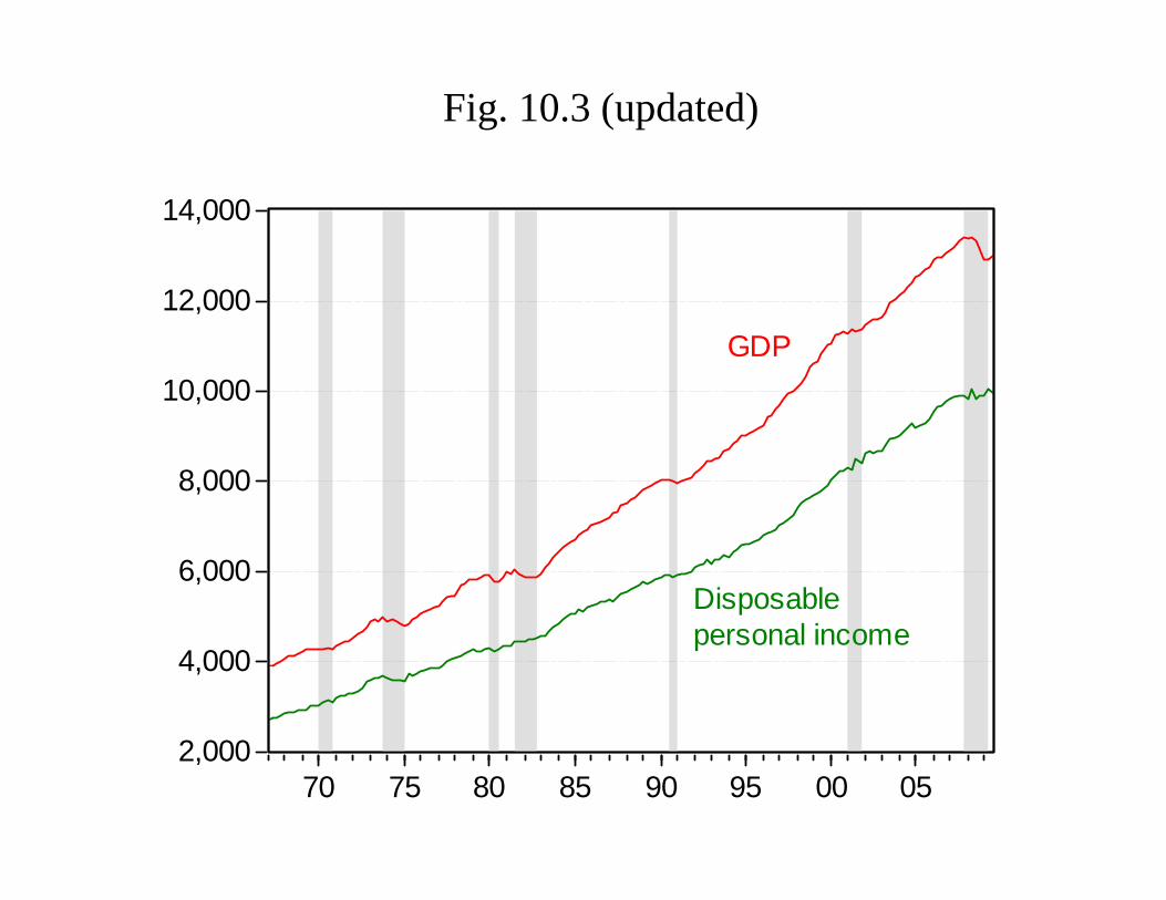
– GDP is about 40 percent greater than personal disposable income.

• The difference between GDP and personal disposable income shrinks during recessions and expands during booms.

2,000

4,000

6,000

8,000

10,000

12,000

14,000

70 75 80 85 90 95 00 05

GDP

Disposablepersonal income

Fig. 10.3 (updated)

The Relation between Real Disposable Income and Consumption

• Consumption fluctuates less than real GDP because disposable income fluctuates less than GDP.

Can all consumption behavior be explained by current personal disposable income, as the simplest consumption function would suggest?

1 , 0 0 0

2 , 0 0 0

3 , 0 0 0

4 , 0 0 0

5 , 0 0 0

6 , 0 0 0

7 , 0 0 0

8 , 0 0 0

9 , 0 0 0

1 0 , 0 0 0

2 ,0 0 0 4 ,0 0 0 6 , 0 0 0 8 ,0 0 0 1 0, 0 00 1 2 ,0 0 0

D IS P IN C 0 5

CO

NS0

5

C = -3 6 2 .8 + 0 . 9 7 Y d

Fig. 10.4 (updated)

The Relation between Real Disposable Income and Consumption

The straight line from the previous figure suggests:

C = 0.97*Yd– This is the simple consumption function; the

marginal propensity to consume (MPC) is 0.97.

– On average, the U.S. public spends about 97% of its disposable income on consumption goods and saves 3%.

The Relation between Real Disposable Income and Consumption

• Consumption is sometimes less and sometimes greater than predicted by the simple consumption function. The errors are given by the equation:

Error = C + 326.2 - 0.97*Yd

and are measured by the vertical distancesbetween the line and the dots in Figure 10.4

(updated).• The simple consumption function seems to

give a surprisingly good description of consumption.

10.2 DEFECTS IN THE SIMPLE KEYNESIAN CONSUMPTION

FUNCTION

• Although the errors in Figure 10.4 appear small, for some purposes (such as forecasting or policy analysis) they are actually quite large.

– A more revealing picture of the errors is found in the next figure:

-200

-100

0

100

200

70 75 80 85 90 95 00 05

Error in SimpleConsumptionFunction

Figure 10.5 (Updated)

Short-Run versus Long-Run Marginal Propensity to Consume

• On average, consumption is smoothed out compared with disposable income; consumption fluctuates less than disposable income.

– This phenomenon can be detected and illustrated by using the concept of the long-run and short-run marginal propensity to consume.

Long-Run Marginal Propensity to Consume

• The long-run marginal propensity to consume tells us how much consumption increases over the long run when personal disposable income rises.

• The short-run marginal propensity to consume tells us how much consumption rises over the short run (during one year or one business cycle) when disposable income rises.

10.3. THE FORWARD-LOOKING THEORY OF CONSUMPTION

• Permanent-income theory developed in the 1950s by Milton Friedman

• Life-cycle theory developed independently at about the same time by Franco Modigliani– The two theories are closely related, and

have served as a foundation for most of the rational expectations research on consumption in recent years.

FORWARD-LOOKING THEORY

• Individual consumers are forward-looking decision makers.

• The life-cycle theory emphasizes a family looking ahead over its entire lifetime.

• The permanent-income theorydistinguishes between permanent income, which a family expects to be long lasting, and transitory income, which a family expects to disappear shortly.

Intertemporal Budget Constraint

• The family faces an intertemporal budget constraint that limits its consumption over the years.

• Assets at the beginning of next year = Assets at the beginning of this year+ Income on assets this year + Income from work this year - Taxes paid this year - Consumption this year

Intertemporal Budget Constraint

• At = Assets at the beginning of year t• R = Interest rate on assets• Et = Income from work during year t• Tt = Taxes during year t• Ct = Consumption during year t.The intertemporal budget constraint can be

written as follows: At+1 = At + RAt + Et - Tt - Ct. (10.3)

Preferences: Steady Rather than Erratic Consumption

• A consumption plan is feasible if it does not involve an impractical asset position at any time in the future.

• Many different consumption plans are feasible. As long as the family is careful not to consume too much, it has a wide choice about when to schedule its consumption.

Preferences: Steady Rather than Erratic Consumption

The forward-looking theory of consumption assumes that most people prefer to keep their consumption fairly steady from year to year.

Given the choice between consuming $10,000 this year and $10,000 next year, as against $5,000 this year and $15,000 next year, people generally choose the even split.

Consumption Smoothing

The MPC out of Temporary versus Permanent Changes in Income• How does consumption change when

disposable income changes? • For forward-looking consumers, the

answer depends on how long the change in income will last; in particular, whether the change is viewed as temporary or permanent.

• The change in consumption is much larger when the change in disposable income is viewed as permanent.

Anticipated versus Unanticipated Changes in Income

• If the change were anticipated, then the family would adjust its plans in advance.

• Consumption would change before the change in disposable income occurred.

10.4. HOW WELL DOES THE FORWARD LOOKING THEORY

WORK?

• The key point of the forward-looking theory of consumption is that the marginal propensity to consume from new funds depends on whether the new funds are a one time increment or will recur in future years.

The Short-Run and Long-Run MPC: A Rough Check of the Theory

• The simple consumption function ignores that the short-run marginal propensity to consume is less than the long-run marginal propensity to consume.

• Consumption does not increase as much with income over short-run business cycle periods as over long-run growth periods.

Ando-Modigliani: Assets in the Consumption Function

• Assets as well as disposable income matter.

• As net wealth declines, consumption will decline.

• Book estimates b2 = 0.06.

ttdt AssetsbYbC 2,1 +=

7.6

8.0

8.4

8.8

9.2

16.0

16.4

16.8

17.2

17.6

18.0

70 75 80 85 90 95 00 05

Log Consumption[right scale]

Log HouseholdNet Worth[right scale]

Where Do We Stand Now?• Economic research in recent years has

led to more revealing tests of the forward-looking theory and raised puzzling new questions

• Three strands of the new research: the use of rational expectations to measure future income prospects, the analysis of data on the histories of thousands of individual families, and case studies of particular economic policy “experiments.”

Where Do We Stand Now?• The forward-looking theory of

consumption works much better than the simple consumption function.

• There are, however, problems with the forward-looking theory with rational expectations.

• The most important problem is that consumption is more responsive to temporary changes in income than the forward-looking theory predicts.

Refinements to the Forward Looking Model

• Precautionary Savings• Consumers face uncertain future labor

income• Consumers are impatient• They place more weight on what is

happening today than on what they expect to happen in the future.

Refinements to the Forward-Looking Model

• Liquidity constraints: - Consumers cannot borrow as easily as

the forward-looking model suggests.

- For example, if you are currently a student, you cannot borrow enough against the expectation of your income after you graduate to completely smooth your consumption.

Refinements to the Forward-Looking Model

• Precautionary savings and liquidity constraints can both explain:

- Why the marginal propensity to consume out of temporary changes in income is higher than predicted by the forward-looking theory.

- Why the marginal propensity to consume out of permanent changes in income does not quite equal 1.

10.5. REAL INTEREST RATES, CONSUMPTION, AND SAVING

• The real interest rate is the relative price between present consumption and future consumption.

• If the real interest rate is high, people face an incentive to defer spending.

• While theory predicts that high real interest rates increase saving and decrease consumption, there is not strong empirical confirmation.

10.6 Implications for the IS Curve• Some of the factors considered in this chapter

make the IS curve steeper, but others make it flatter.

• According to the forward-looking theory of consumption:

- The shift in the IS curve should be much larger if the tax cut is permanent rather than temporary.

- A purely temporary tax cut would have a very small effect on the IS curve.

- The IS curve shifts to the right in response to an expectation of further tax cuts. Future tax cuts stimulate consumption today because lifetime disposable income has increased.