1

Economic Volatility: Does Financial Development, Openness and

Institutional Quality Matter In Case of ASEAN 5 Countries Hazman Samsudin

1,2*

1 PhD in Economics student at Faculty of Business and Government, University of Canberra, Canberra, ACT 2601

2 Tutor at Faculty of Management and Economics, University Malaysia Terengganu, Malaysia 21030

*email: hazman.s@umt.edu.my / Hazman.Samsudin@canberra.edu.au

JEL Classification: C23, E02, F44, G20, O16.

1. Introduction

In recent years there has been substantial attention on the link

between economic volatility and financial development together

with financial and trade openness policy as well as the role of

institutional quality. Moreover, a series of financial crises have

occurred and put the slowed down which saw the financial

meltdown of the major economy of the world such as the Euro

zone and previously East Asia 1997 financial crisis and it was

said to associate with the rapid financial development together

with the effect of openness instability as well as institutional

quality factor. The state of financial conflict has raised the

question of rationality behind the openness policy, the role of

institutions as well as financial sector development and has fuel

the fire on the topic and heat up the debate.

Having said that, this study attempt to shed the light on the link

between economic volatility with financial development and

openness in both segments which is trade and financial along

with the role of institutional quality in ASEAN-5 countries

namely Indonesia, Malaysia, Philippines, Singapore and

Thailand. In recent years ASEAN-5 have been subjected to

rapid economic growth and several dramatic economic

fluctuation has taken place which made a study on economic

volatility on ASEAN-5 very tempting. ASEAN also have gone

through several economic integration phase such as the

establishment of ASEAN Free Trade Area (AFTA), ASEAN

Comprehensive Investment Agreement (ACIA) and Chiang Mai

initiatives and the increasing level of economic integration in

trade and financial sector among them as well as international

market such as China, Australia and New Zealand also have

made this topic very interesting to discuss especially at how far

the integration have affected their aggregate economic

volatility. Moreover, the impact of financial and institutional

sector reform especially during the privatization and

liberalization era of the 80’s as well in the aftermath of 1997

crisis need to be asses the implication on economic volatility.

2. Selected literature review

In witnessed the effect of globalization and financial contagion,

many have reconsidered the pros and cons of financial

liberalization due to the effects from capital controls removal

where they are often associated with volatility (Schmukler,

2003). According to the same author capital controls removal

often associated with economic volatility and according to Ang

and McKibbin (2006), liberalization may increase economic

volatility in financial system and hence trigger financial crises if

carried out improperly. In addition, Stiglitz (2000) explained

that the increasing recurrent of financial crises may have

something to deal with financial liberalization since capital

flows are cyclical in nature which will deteriorate economic

swing. Moreover, Aghion et al. (2004) explained that,

liberalization may destabilize economy where it will speed up

the persistent phase of growth with inflows of capital which

then followed by economic collapse and capital flight.

On the other hand, trade openness is also found to be unstable

and may cause volatility hence leading to recession (Razin et

al., 2003). Trade openness encourages specialization of

production based on comparative advantage assumptions where

it will make an economy more susceptible towards industry

specific shocks (Kalemli Ozcan et al. 2003). Greater openness

to world goods markets may also encourage domestic economic

instability due to reliant on international environment such as

exchange rate (Arora and Vamvakidis, 2004; Blankenau et, al.,

2001; Rodrik, 1998) hence lead to sensitive susceptibility to

external shocks.

Furthermore, it’s been argued that government institutional also

may be affected by political influence and it may be misused by

political power to favor their cronies based institutions which

will not bring the economy up to their optimum efficiency

hence risking the economy towards crises moreover in the state

of liberalization. For instance, Stigler (1971) as stated in

Aggarwal and Goodell (2009), suggest that the supervision

approach by official to banking regulation will make things

worst rather than good because of interference with market

forces which it indicate that strengthening institutions will only

lead to more intervention thus slowing economic activities and

risking for excessive volatility occurrences. In other words,

strengthening institutional quality could lead towards paradox

of enrichment1.

Mean while, an increase in financial development could lead

towards more economic volatility due to adverse selection and

moral hazard which caused by increase in asymmetric problem

where possibilities of failure to detect profitable investment still

could be from abundance of financial instruments and

sophisticated financial system especially when financial sector

development is at intermediate level. Moreover, Acemoglu and

Zilibotti (1997) illustrate that the interaction of investment

indivisibility which followed by inability to diversify risk may

magnify economic volatility. On the other hand, monetary

shocks also could increase the chances of economic volatility

moreover when monetary policies often changes which could

refer to rapid intervention by government (Beck et al, 2000).

While others such as Kiyotaki and Moore (1997) point out that

the imperfection of capital market could intensify the effects of

short run productivity shocks and make them more persistent.

However, it is also been argue that a well developed financial

system may have the ability of absorbing shocks easily through

1 Paradox of enrichment is the term used in population ecology to describe the collapse of population

system when abundance of resources was given. In this sense, over strengthening institutional such as legal

framework, may lead towards piling up more barriers in term of regulations which may negatively affect

capital flow thus triggering volatility. Another example also could be rapid government intervention may

lead towards frequent changing in regulations which is something might not preferred by investors.

2

the capability of matching savers and investor easily at

minimum amount of time thus avoiding capital flight which

could meant for excessive volatility control. For instance, the

main role of financial development is to lead and link between

the deficit unit and the surplus unit which in turn may benefit

the whole economy through the process of effectively turning

saving into investment (Chinn and Ito, 2006 and Levine, 2005).

According to Kose et al., (2006) this effects could also reduced

volatility by means of providing access to capital which may

assist in diversifying production base. Furthermore, financial

system efficiency in processing information, monitoring and

managing risk, supplying information about profitable ventures,

diversify risks, and facilitate resource mobilization may lead

towards effective investment which could decrease the chance

of excessive volatility occurrences. Therefore, a well developed

financial system assists in improving capital structure and the

efficiency of resource allocation, promoting thereby long run

economic growth (Kim et, al., 2009) and reduce economic

volatility (Ahmed and Suardi, 2009). According to Chinn and

Ito (2006), this is due to the nature of financial development in

enhancing asymmetric information, lessens the cost of

transaction and information, better corporate governance and

facilitating risk management thus improving returns as well as

reducing the cost of capital and investment respectively.

Moreover, Kim et. al. (2009) added that financial institutions as

well as financial market may also provide information on

profitable ventures, diversify risks and facilitate resource

mobilization. These effects on financial development has by

large reduce economic volatility due to increase in confidence

and certainties on return thus increase the level of investment

and hence promote economic growth (Pindyck, 1991).

On the other hand, openness also might have a negative

relationship with economic volatility which means that, a more

open an economy on international market, the lower the

economic volatility will be. An open economic in both segment

which is trade and financially could have better risk sharing and

well diversified investment portfolio which could be vital in

reducing the impact of economic shocks. This is also was in line

with Bekaert et al., (2006) which also illustrate that financial

opening does reduce volatility by improved risk sharing. On the

other hand openness also may increase the amount of

international portfolio investment flows which consecutively

may increase the liquidity of domestic stock markets which

refers to increase in total money supply where this could be vital

for economic development and also with the presents of foreign

entity might also facilitate access to international financial

markets. Therefore open economy could facilitate volatility. As

been discussed before, by allowing for financial opening

specifically by lifting the restrictions on foreign portfolio flows

are likely to improve stock market liquidity and also by

permitting the presence of more foreign bank will increase the

domestic banking system efficiency. According to Levine

(2001), an increase in financial system efficiency for both

banking and financial market may in turn equip them with

capability to deal with an increase in volatility where they are

more capable in absorbing economic shock.

On the other hand, trade openness also may affect volatility

negatively. Greater integration through openness could stabilize

the consumer price which could bring the price level at

optimum which matches with the international price level hence

reducing the chances of inflationary shocks. In other words,

openness in trade segment may improve resource allocation,

lowers consumers’ prices and leads towards more efficient

production thus reducing volatility. Moreover it also encourages

the technological transfer which may result in productivity

improvements thus increase economic development which

could mean a reduced impact on volatility. Mean while, trade

openness also may increase industries specialization and

according to Razin and Rose (1992), an increase in trade with

increased specialization of intra industry would lead towards a

declining in output volatility due to greater volume of

intermediate inputs trade.

Mean while, institutional quality also could negatively affect

economic volatility. Institutional quality may reduce volatility

by mean of increase in bureaucratic quality which could be vital

in speed up any government work process, transparency thus

ensuring return in investments, better legal framework making

any investments decision easier with less uncertainties and less

risk of contract repudiation could reduce the risk of capital

flight. For instance, legal protections for creditors and the level

of credibility and transparency of accounting systems are also

likely to affect economic agents financial decisions (Beck and

Levine, 2004), (Claessens et, al., 2002), (Caprio et, al., 2004),

and (Johnson et, al., 2002) and also lowering volatility as they

might reduce asymmetric information (Silva, 2002) as well as

increase the level of investors’ confidence (pindyck, 1991).

With given the relationship between economic volatility and it

determinants are still ambiguous and the study focusing on this

matter is still relatively thin, this study tends to dig more

conclusions on this topic.

3. Area of study

ASEAN-5 namely Malaysia, Indonesia, Thailand, Singapore

and The Philippines are being chosen as the case of study. It is

agreed that the study for all the members of ASEAN countries

will be more comprehensive; however, data gathering process is

not an easy task in a country such as Myanmar, Brunei, Laos,

Cambodia and Vietnam in term of data availability. In addition,

due to the fact that the GDPs of these countries would comprise

nine-tenths of ASEAN’s overall GDP, a study on the main

player of ASEAN members that is ASEAN-5 hope to be

sufficient in order to capture the determinants of economic

volatility in the said region therefore allowing for comparison

study.

Moreover, if ASEAN counted as a single market, it would be a

market of 584 million people and 72 percent of it is accounted

for by the population of the ASEAN-5. This came third in the

world after China and India and, plus, ASEAN has a combined

GDP of US$1,504 billion where 90 percent of it was a

contribution of ASEAN-5 which is second to China’s in

emerging Asia2.

ASEAN 5 as an emerging economies did introduced continuous

and prompt growth, with remarkable structural change and

considerable enhancement in standards of living (Asian

Development Bank, 1997) throughout the years. Furthermore,

due to recent increase in economic integration and negotiation

among them (for instance AFTA, AIC, Chiang Mai initiatives

and etc) as well with international economies (for instance

AANZFTA), an economic review on how it have shape the

level of financial sector development and the level of openness

as well as its institutional quality have affect their economic

volatility looks very interesting to discuss. Therefore an

economic review on this matter is essential especially in

2 Data are obtainable from ASEAN community in figures (ACIF) 2009

3

assessing the effectiveness of recent economic integration and

financial arrangements as well as policy decision.

4. Some issues in existing literature

In reviewing the literature, it is found that the lack of past

studies for individual ASEAN-5 countries. Most of the past

studies are conducted based on cross country or panel data

analysis. Therefore, the present study attempts to fill up this gap

on the literature. The advantages of having individual country

studies would give us a better finding because definitely for

economic policies, historical and institutional factors are equally

important. Other researchers such as Hasan et, al., (2009) also

point out that most studies especially regarding of institutional

and political influences employ cross country data which is hard

to interpret due to the richness in historical experiences, norms

and institutional contexts. In addition, the data on income or on

inequality in different countries are not comparable, either

because the purchasing power parity adjustments necessary for

such comparisons are not reliable or because the methodologies

underlying different countries’ numbers are too diverse to be

pooled together, or both. Therefore, his study will fill the gap by

undertaking individual country study where an individual

country studies will allow for comparison studies in which

where policies will work best.

Furthermore, most of past studies highlighted the relationship

between financial development, openness and institutional

quality institutional quality with economic growth while less of

them shed the light on economic volatility. It’s been argued that

even if volatility is considered to have as a second ordered

issue, their effects on growth could indirectly regards as first

order welfare implications (Kose et. al., 2006). Therefore, a

study on the effect of volatility has to be taken seriously

moreover in recent years where there has been a substantial

issue regarding economic volatility which involving the level of

financial sector development and the level of openness as well

as the crucial role of institutional quality.

In addition, according to IMF (2003), they point out that

financial liberalization should go along together with trade

liberalization in assuring successful financial development

where the main role from financial institutions are barely

needed to reduce the trade transactions cost. It has been argued

that with increasing globalization of trade and financial flows, a

fully integrated economy cannot exist unless supported by a

well functioning financial sector, and vice versa. International

trade can flourish when essential trade related financial services

and credit are available. On the other hand, trading opportunities

help create demand for financial services and instruments, thus

enhancing the development of financial system. However, as

been mention above, China’s and India’s market rely heavily on

trade openness but not complete financial openness and

nevertheless their economies are performing well which given

doubt on the hypothesis made by IMF (2003) and Rajan and

Zingales (2003). Having said that, it is crucial to check the

situation in the case of ASEAN-5 and therefore, this study will

also test the simultaneous openness hypothesis.

With those address issues in past literature, this study tend to fill

the gap where this study will examine the relationship between

economic volatility with financial development and openness in

both segment simultaneously as well as the role of institutional

quality in ASEAN 5 countries by utilizing time series data

analysis for each country.

5. Derivation of Data

For the purpose of the study, aggregate economic volatility will

be constructed by utilizing the principal component analysis.

One of the benefits by employing this method is it can

overcome the possibilities of multicollinearity and

overparametrization as an overall indicator of aggregate

economic volatility. However, before coming into the principal

component analysis, it is better to define the terms volatility in

the first place. The term volatility can be defined as the

deviation of real time series data from its mean value overtime.

Therefore, volatility in this study is measured by taking the five

years rolling standard deviation of each proxy.

An aggregate economic volatility can be captured through four

perspectives which are the consumption growth volatility,

output growth volatility, external volatility and internal

volatility. Consumption growth volatility is proxy by the

standard deviation of total consumption (Lσtc) where total

consumption growth rate are the total of private consumption

plus the government consumption. In most cases of developing

countries, government consumption has been very influential

and in mass volume, therefore would have an implication

towards volatility. The standard deviation of the ratio of total

consumption growth rate is simply to measure the effectiveness

of consumption smoothing relative to output volatility.

Output growth volatility on the other hand is proxy by standard

deviation of GDP per capita (LσGDP per capita) where it may

depicts the cyclical variability in net factor income flows which

hold the effects of international risk sharing on national income

due to market reforms. Mean while, external shock volatility is

proxy by the standard deviation of term of trade (Lσtot) where it

may represent the external shocks factor where the term of trade

has been a factor in measuring social welfare and the growing

trade activities in the region would have an implication on

volatility.

Internal shock volatility is proxy by standard deviation of

government expenditure (LσGovex) where government

expenditure would provide somewhat cyclical behavior and

could have an instant effect on the response of private

consumption to macroeconomic policy (Ahmed and Suardi,

2009) which can be used to capture the domestic shocks.

Therefore an aggregate economic volatility is developed based

on those perspectives of volatility. The summary of the

principal component analysis on aggregate volatility is as in

table 1.

From the analysis, it indicates that most of the eigenvalues are

able to capture more than 56% in case of Indonesia and

Malaysia, Singapore 54%, Thailand 58% and 38% in

Philippines. It is normally the first principal component (PC1)

which will tell the most of data variation and each of the

succeeding analysis will have the highest variance possible with

the constraint it would be orthogonal to the previous component

analysis. Therefore, the construction of aggregate economic

volatility data is constructed based on the vector 1 for every

country and the vector value for each variable will be scale

accordingly3. The aggregate volatility data will then be derive

after taking account the weight of each aggregate volatility

component and denote with Lvol.

Table 1: Aggregate volatility principal component summary

Indonesia PC1 PC2 PC3 PC4

Eigenvalues 2.259648 0.882693 0.643353 0.214306

3 The scaling of each variables vector value is done by doing simple average of total vector value

4

% Of variance 0.5649 0.2207 0.1608 0.0536 Cumulative % 0.5649 0.7856 0.9464 1

Variable Vector 1 Vector 2 Vector 3 Vector 4

Lσtc 0.520035 0.480896 0.426341 -0.56262

Lσgdp per capita 0.45364 0.42623 -0.75313 0.212918

Lσtot 0.577092 -0.21096 0.417478 0.669458

Lσgovex -0.43674 0.736589 0.277022 0.43584

Malaysia PC1 PC2 PC3 PC4

Eigenvalues 2.278689 1.023897 0.499653 0.197761

% Of variance 0.5697 0.256 0.1249 0.0494

Cumulative % 0.5697 0.8256 0.9506 1

Variable Vector 1 Vector 2 Vector 3 Vector 4

Lσtc 0.483134 0.515294 0.567277 -0.42338

Lσgdp per capita 0.463977 0.486951 -0.7243 0.151661

Lσtot 0.577597 -0.31083 0.305557 0.690219 Lσgovex -0.46657 0.633038 0.245415 0.566874

Philippines PC1 PC2 PC3 PC4

Eigenvalues 1.53398 1.164866 0.887147 0.414007

% Of variance 0.3835 0.2912 0.2218 0.1035 Cumulative % 0.3835 0.6747 0.8965 1

Variable Vector 1 Vector 2 Vector 3 Vector 4

Lσtc 0.718816 -0.03915 -0.11406 0.684661 Lσgdp per capita 0.212413 0.668927 -0.64931 -0.29293

Lσtot 0.577401 0.20296 0.619656 -0.49137

Lσgovex -0.32372 0.714011 0.425921 0.45165

Singapore PC1 PC2 PC3 PC4

Eigenvalues 2.166626 0.841703 0.66755 0.324121

% Of variance 0.5417 0.2104 0.1669 0.081

Cumulative % 0.5417 0.7521 0.919 1

Variable Vector 1 Vector 2 Vector 3 Vector 4

Lσtc 0.434509 -0.546 0.711217 0.085165

Lσgdp per capita 0.597383 0.102872 -0.19362 -0.7714

Lσtot 0.522493 -0.29661 -0.60893 0.517906

Lσgovex 0.425837 0.776738 0.293059 0.3598

Thailand PC1 PC2 PC3 PC4

Eigenvalues 2.322742 0.865502 0.606705 0.205051

% Of variance 0.5807 0.2164 0.1517 0.0513

Cumulative % 0.5807 0.7971 0.9487 1

Variable Vector 1 Vector 2 Vector 3 Vector 4

Lσtc 0.604046 -0.08581 0.208149 0.764487

Lσgdp per capita 0.320813 0.923306 -0.18646 -0.09909

Lσtot 0.558549 -0.14897 0.545735 -0.60664

Lσgovex -0.46929 0.343442 0.789988 0.194256 Note: Lσtc = log standard deviation of total consumption, Lσgdp per capita = log standard deviation of

GDP per capita, Lσtot = log standard deviation of term of trade and Lσgovex = log standard deviation of

government expenditure

The second variable which is aggregate financial development

also goes through the same process of Principal component

analysis. The aggregate financial development index are

constructed based on the data of domestic credit to private

sector divided by nominal GDP (Ldome), M2 over the nominal

GDP (Lm2), the ratio of bank domestic asset to total assets of

bank and central bank (Ldbacba), stock market capitalization

(Lstmcap), total value stock traded (Lstval) and stock market

turnover (Lsto). Basically this data follow the standard

measurements of financial development as in Beck et. al.,

(2000) where the first three indicators reflect the banking sector

development and the last three indicate the market sector

development. Each of these variables captures different aspect

of financial development.

For instance, the first proxy represents overall development in

private banking markets, where; it excludes credit granted to the

public sector and credit issued by the central bank. The reason

of excluding the loans issued to governments and public

enterprise is, it is often argued that the private sector is able to

utilize funds in a more efficient and productive manner which

reflects the extent of efficient resource allocation. Second

proxies also known as liquidity liabilities, in which it was

largely used in measuring financial depth where it was designed

to depict the overall size of the formal financial intermediary

sector and provide information regarding the degree of

transaction service provided by the financial system. However,

some have argued that these are not good proxies as they posses

several weaknesses4. Nevertheless, for the purpose of this study,

each proxy’s captures fairly different aspect of financial

development, therefore neglecting this proxy should not be the

case. The third proxy of bank based measurement of financial

indicator is the bank assets which measure the degree of

importance of each financial intermediary and domestic bank

efficiency in turning society savings towards more profitable

investment opportunities.

As for the market based indicator which covers the development

of non bank and equity sector, they are made up based on three

proxies which is stock market capitalization (Lstmcap), total

value stock traded (Lstval) and the stock market turnover (Lsto).

The first proxy reflects the size of the equity markets it shows

the share of domestic companies over GDP. Second and third

proxies define the dynamism or the activeness of stock market

(Beck et, al., 2000), where the total value stock traded shows the

total market value of shares traded in term of GDP and stock

market turnover ratio measure the transaction of stock towards

the market size where it is often used as market liquidity

measures. All of these measurements are specified in term of

ratio to GDP.

Therefore the aggregate financial development index is

constructed based on these 6 variables. The summary of the

principal component analysis is as in table 2. As clearly seen, in

the case of Singapore there is only five principal components

analysis took place. This is due to the one of the variable which

is the bank domestic asset to total assets of bank and central

bank (LDbacba) is problematic thus the variables is taken out of

the construction of aggregate financial development5.

Nevertheless, for the rest of the country there has been no issue

with the data. Based on the results, it indicate that more than

56% variation of the data are captured in the first principal

component eigenvalues in Indonesia while 61% in Malaysia,

54% in Philippines, 55% in Singapore and 71% in Thailand.

This shows that the combination values of each variable in

vector 1 for every country are able to reflect more than half of

total 6 variables. The vector values of each variable will be

scaled to determine the weight it will carry in construction the

aggregate financial development data which is denoted with Lfd.

Table 2: Aggregate financial development principal

component summary

Indonesia PC1 PC2 PC3 PC4 PC5 PC6

Eigenvalues 3.334247 1.57847 0.684444 0.34908 0.036211 0.017548

% Of Variance 0.5557 0.2631 0.1141 0.0582 0.006 0.0029

Cumulative % 0.5557 0.8188 0.9329 0.991 0.9971 1

Variable Vector 1 Vector 2 Vector 3 Vector 4 Vector 5 Vector 6

LDome 0.269068 0.662642 -0.28049 -0.06891 -0.39407 -0.4998

LM2 0.462444 0.055617 -0.60489 -0.26767 0.174857 0.561198

LDbacba -0.14455 0.723949 0.315932 0.284605 0.297423 0.430964

LStmcap 0.506153 -0.11256 -0.04498 0.566221 0.534263 -0.35082

LSto 0.432849 0.056268 0.575911 -0.63526 0.244322 -0.12063

LStval 0.499304 -0.13369 0.349182 0.344155 -0.61688 0.334526

Malaysia PC1 PC2 PC3 PC4 PC5 PC6

Eigenvalues 3.651677 1.266792 0.517539 0.337203 0.177745 0.049043

% Of Variance 0.6086 0.2111 0.0863 0.0562 0.0296 0.0082

Cumulative % 0.6086 0.8197 0.906 0.9622 0.9918 1

Variable Vector 1 Vector 2 Vector 3 Vector 4 Vector 5 Vector 6

LDome 0.354346 0.406205 0.724358 0.424007 -0.02001 -0.06753

4 Some have argued that liquidity liabilities fail to capture the role of the financial system to direct funds

from depositors to investment opportunities. Furthermore, the monetary aggregates of foreign fund in

financial system are insufficient measures of financial development. It also potentially admits double

counting. Further detailed see Ang and McKibbin (2006) and Kim et. al., (2009) 5 Lots of missing data in case of Singapore where data observation from 1972 until 1999 were missing.

However the data was made available again in year 2000 onwards.

5

LM2 0.459608 0.24769 -0.3338 -0.14468 -0.66548 -0.39012

LDbacba 0.335549 0.585863 -0.42036 -0.06994 0.579068 0.165097

LStmcap 0.471863 -0.20813 0.22892 -0.48917 -0.14107 0.649952

LSto 0.383111 -0.42914 -0.33924 0.706844 -0.01503 0.232648

LStval 0.42565 -0.45048 0.14035 -0.23554 0.448653 -0.5826

Philippines PC1 PC2 PC3 PC4 PC5 PC6

Eigenvalues 3.209996 1.313401 0.850685 0.433724 0.147684 0.04451

% Of Variance 0.535 0.2189 0.1418 0.0723 0.0246 0.0074

Cumulative % 0.535 0.7539 0.8957 0.968 0.9926 1

Variable Vector 1 Vector 2 Vector 3 Vector 4 Vector 5 Vector 6

LDome 0.436796 0.18728 0.258249 -0.7939 -0.27778 0.002187

LM2 0.085981 0.755346 0.459556 0.238342 0.390802 0.036526

LDbacba 0.473467 0.263609 -0.233 0.450062 -0.58327 -0.3306

LStmcap 0.517392 -0.01719 -0.35181 0.096728 0.204338 0.74641

LSto 0.23496 -0.48865 0.734764 0.31702 -0.1815 0.180811

LStval 0.504722 -0.29294 -0.06461 -0.02248 0.595999 -0.54731

Singapore PC1 PC2 PC3 PC4 PC5

Eigenvalues 2.768573 1.116991 0.902719 0.163767 0.04795

% Of Variance 0.5537 0.2234 0.1805 0.0328 0.0096

Cumulative % 0.5537 0.7771 0.9577 0.9904 1

Variable Vector 1 Vector 2 Vector 3 Vector 4 Vector 5

LDome 0.35013 0.733553 0.077647 0.573725 -0.06418

LM2 0.522529 0.356684 -0.07325 -0.76978 -0.04256

LStmcap 0.301967 -0.21382 0.875441 0.005406 0.310917

LSto 0.494727 -0.29425 -0.46966 0.209007 0.635923

LStval 0.518107 -0.44986 -0.04037 0.185909 -0.70214

Thailand PC1 PC2 PC3 PC4 PC5 PC6

Eigenvalues 4.236854 0.910026 0.444637 0.226055 0.130725 0.051703

% Of Variance 0.7061 0.1517 0.0741 0.0377 0.0218 0.0086

Cumulative % 0.7061 0.8578 0.9319 0.9696 0.9914 1

Variable Vector 1 Vector 2 Vector 3 Vector 4 Vector 5 Vector 6

LDome 0.454667 -0.04706 0.221646 0.187796 -0.84016 0.028266

LM2 0.426536 -0.23838 0.49568 0.384408 0.447086 -0.40974

LDbacba 0.437682 -0.04893 0.300205 -0.78432 0.152843 0.278208

LStmcap 0.438581 -0.21257 -0.44753 0.351812 0.230705 0.620627

LSto 0.206424 0.939694 0.119761 0.169696 0.132535 0.116877

LStval 0.429901 0.101755 -0.63279 -0.2219 -0.00964 -0.59588

Note: LDome = log domesticcredit to private sector, LM2 = log M2, LDbacba = bank domestic asset to

total assets of bank and central bank, LStmcap = log stock market capitalization, LSto = log stock market

turnover ratio and LStval = log total value stock traded

The financial openness data in this study will be proxy by the

“De facto” and “De jure”. Financial openness measured by “De

facto” is the financial globalization indicator constructed by

Lane and Milesi Ferretti (2006) and this indicator is defined as

the volume of a country's foreign assets and liabilities as a

percentage of GDP. Therefore “de facto” might reflect the

country history of financial openness. Mean while, “De jure”

measurement of openness is the one develop by Chinn and Ito

(2007) where they derive the index of capital account openness

(KAOPEN). This measurement is build from four binary

dummy variables where it reflects the cross border financial

transactions restrictions which reported in the IMF's Annual

Report on Exchange Arrangements and Exchange Restrictions

(AREAER). These binary variables are then reversed to make it

equal to unity which reflects the perfect free market without

restrictions. Therefore the “de jure” data is a dummy variable

with range between 0 and 1 where the closer the value to 0

indicate that the country are practicing lots of restriction or

protective policy while the closer to 1 indicate that the country

is more open with less barriers.

However, the dummy variables produced are by utilizing the

principal components analysis which may suffer from

measurements error where some variation of the underlying data

may not be documented for. Furthermore, the data also may

suffer from the enforcement issue. If let say a country have

lifted up the barriers doesn’t mean it would imply greater capital

account openness if the right to engaged is not fully utilized in

international transaction thus it would over state the actual level

of capital openness.

Nevertheless, it’s been argued that the “de jure” measurements

have a better grounded theory than “de facto” especially when

“de jure” is more strongly associated with the decision to open

up an economy towards capital flows. This is contrast with the

“de facto” measurements of openness where the measurements

may bias towards other underlying factors of capital flows such

as future prospect where it may increase the question of

reliability of “de facto” as a proxy of capital account openness.

Nevertheless “de facto” measurements are less vulnerable

towards political factors influence since the decision to increase

or reduce openness may be influenced by some interest groups.

Having said that, despite the weaknesses of the measurements, it

is actually the strength of the measurements and as been

mentioned earlier, “de facto” measurements may reflect the

country historically background, geographic and international

politics which may be out of policy maker control thus less

issue with influence of political factor compared to “de jure”

measurements. Therefore, some researchers argue that the “de

facto” measurements might be more relevant for pure test of

financial openness hypothesis where it seems to reflect the true

level of openness or outcome based measurements. On the other

hand “de jure” measurements of openness may be close related

towards the policy based financial openness measurements.

Due to the both measurements might have their own strength

and weaknesses as well as both measurements also depict

financial openness in different perspective which is outcome

based and policy based, both measurements of financial

openness will be employ in this study. Both measurements are

denoted as Ldejure and Ldefacto respectively.

The third variable which is included in this study is the trade

openness which is denote as Lto where it is defined as annual

data on real GDP per capita, converted to US dollars at constant

2000 is measured by the ratio of total trade to GDP will be the

proxy for trade openness. The measurement of trade openness is

apparently less complicated and straightforward compare to

financial openness measurements.

The fourth variable is the institutional quality indicator.

Actually there are numerous of institutional quality indicator

have been made available and it can be divided in to two types

which is the objective measurements and the subjective

measurements. Objective measurements can be obtained by

employing the Contract Intensive Money (CIM) which has been

developed by Clague et. al., (1997)6. Besides its strength such as

abundance of data in term of data duration and advantage over

contamination of recent economic situation or performance

knowledge bias by evaluators especially in subjective

measurements, it also contained some weaknesses which is, it

might be a little bit “noisy” as the decision of holding financial

assets might be influenced by other factors such as norms,

expectations based on global and domestic economic situation,

interest rate and the rate of inflation. Having said that, this

variable might not be sensitive towards growth rate when

controlling for inflation and one of the most common

measurement of financial development which is M2 to GDP

where those variables is used in constructing aggregate financial

development indicator in this study.

Therefore, this study will employ the subjective over objective

measurements due the reason stated above. For the purpose of

this study, the subjective measurements of the institutions

quality indicator provided by BERI (Business Environment

Risk Guide) will be used over ICRG (International Country

Risk Guide). This consideration is made based on the

availability of longer time period where the data on ICRG only

6 More information on this can be obtained from “contract intensive money: contract enforcement, property

rights, and economic performance” by Clague et. al., (1997)

6

available starting from 1984 while BERI starts from 1980. This

is due to one of the aim of this study is to analyze the effect of

openness and institutional quality on financial development as

well as the economic volatility by emphasizing the time series

data analysis which means the more the series of the data, the

better the view of the relationship. Therefore, the data from

BERI will be employed in this study to proxy for institutional

quality factor which denoted with Lberi.

Basically the data were made up based on several indicators

such as the degree of privatization, bureaucracy delay, contract

enforcement, communication and transportation, nepotism and

corruption, and the level of legal framework. The degree of

privatization refers to the seriousness of government in

outsourcing or transferring any government activity through

businesses, enterprise, agency, public service or public property

to private sector in achieving better services to support

businesses needs. It also could means as a medium of reducing

red tape which usually exist in government sector and also as a

useful sight of chances of force nationalism in a particular

country. On the other hand, contract enforcement refers to the

extent and the seriousness of government in honoring any

contract that have been made.

Communication and transportation also could make weigh in

building up the institutions quality measurement where it could

be as an indicator in assessing the “facilities for and ease of

communication between headquarters and the operation, and

within the country,” and also as an indicator of transportation

quality which could be important for businesses as well as a

reflection of government efficiency in allocating public goods

and prioritize business activity. According to Knack and keefer

(1995), it is likely that poorer country to have low indicator in

this measurement. Mean while nepotism and corruption is a

measurement of the wrong doings of government official such

as bribe or illegal payment which might be something to do

with licensing, exchange controls, taxation, policy protection

and so forth. The measurement also reflect the level of

prioritize on political connected organization or businesses, one

sided decision due to owing for special payments to government

official and other similar things. The last sub component of

institutional quality is the level of legal framework. Legal

framework can be viewed in two dimensions which is law as

written and the actual practice such as dividend, royalties,

remittances, repatriation of capital, hedging against devaluing

currency and the like of it. Having said that, the differences

between what was written and actual practice depict the level of

willingness to accept the established institutions in making and

implementing laws and adjudicate disputes.

The higher the score for each component indicate the better the

institutions in the particular country. Therefore, by combining

these entire sub components will make an all rounder

institutional quality measurement which may capture at every

different aspect of governance that might influence economic

volatility in a particular country. For the purpose of aggregating,

this paper will follow the method of simple addition aggregating

by Knack and keefer (1995) where all of the indices are given

the same weight. According to the author, even when individual

components of indices are employed, the result doesn’t change

significantly and also when they are compiled with different

weights. While the other issue on bias of employing BERI

database over ICRG should not exist as all of the

subcomponents are very close analogous with each other in term

of the definitions and what is important is the selection was

made base on the needs of the study.

Control variables on the other hand, are also being introduced in

this study. The main reason for introducing the control variable

is to avoid or reduced some of the econometrics problem such

as endogeneity which may arise as a result of measurements

error, autoregression with autocorrelated errors, simultaneity,

omitted variables and sample selection errors.

The first controlled variables are the real interest rate (Lint)

which is suggested to have an impact on the financial sector.

For example, Ang and McKibbin (2006) found that an increase

in real interest rate would have a negative impact on the

financial sector which also consistent with Arestis et al. (2002).

Second controlled variable to be included is the per capita

income (Lincpc) where it is necessary to control the causal

relationship between income and financial deepening. It is

become almost common to include this variable as this variable

are often associated with their contribution towards the

complexity of economic structure (Chinn and Ito, 2005).

The third variable is the inflation rate (Linf) where it is defined

as the rate of changes in CPI in which it is an essential indicator

for macroeconomic stability measurements (Beck et al 2000). It

is an important proxy for unpredictability in inflation as it will

have an impact in decision making particularly in real assets

saving (Chinn and Ito, 2006). The fourth, control variables is

the exchange rate (Lex). It is expected that exchange rate could

possibly trigger volatility as they could distort volume of trade

and capital flows. However to what extent the distortion is still

ambiguous depends on the nature of shock whether it is fiscal or

monetary derives and depends on the exchange rate regime as

well where at the end it could have positive or negative impact

on volatility (Silva, 2002). In this study exchange rate is

measured as the absolute value of the change in exchange rate

which is defined as SDRs per unit of national currency. The last

controlled variable to be included is the government expenditure

to GDP (Lgovex) which also is at best as an indicator of

macroeconomic stability. Government expenditure is vital in

reflecting the impact of public expenditure in distorting private

decisions which in turn will have an effect towards the financial

sector.

Most of the data are obtainable from World Development

Indicator (WDI) except the data for institutional quality

indicator which is obtainable from the Business Environment

Risk Intelligence (BERI) and the openness indicator of “de

facto” are obtainable from Lane and Milesi Ferretti (2006) and

from Chinn and Ito (2007) for “de jure” indicator while the

exchange rate data are obtainable from International Financial

Statistic (IFS) online version. All of the data will be

transformed in logarithm form in order to avoid precision error

measurements and all data will have similar unit of

measurements as well as to reduce widely varying quantities to

much smaller ranges. By transforming into logarithm form also,

the estimated coefficient also will be interpreted as elasticities.

The data will cover from 1970 until 2011.

6. Methodology and Empirical Findings

In order to capture the relationship between volatility with

financial development and the effect of openness in a sound

institutional quality, this model was further setup which can be

viewed as follows:

itit

itititit

CtrLberi

LtoLdefactoLdejureLFdLvol

65

4321 (1)

7

Where, Lvol is volatility, Lfd is financial development, Ldejure

and Ldefacto financial openness and Lto is trade openness,

Lberi is institutional quality, Ctr is set of control variables and ε

is standard error while α and β is the estimated parameter in the

model.

For the purpose of this study the Autoregressive Distributed Lag

(ARDL) bound test to cointegration will be employed to

estimate equation (1). This is because the ARDL method of

estimation will still efficient even if there is a mix level of

stationarity of I(1) or I(0) among the regressors7. Other

advantage of bounds test approach is the method can be applied

for a small sample study8. These are the advantages of using

Pesaran et al.’s (2001) method cover common practice of

cointegration analysis like Engle and Granger (1987) and

Johansen and Juselius (1990). Another important advantage of

the bounds test procedure is that estimation is possible even

when the explanatory variables are endogenous.

However, even though the method allow for mix stationarity

level to be mix in the same model, the regressand should not be

at I(0) level of stationarity and no other variables at I(2) level of

stationarity should incorporated in the same model or otherwise

it may lead towards spurious regression and the presence of

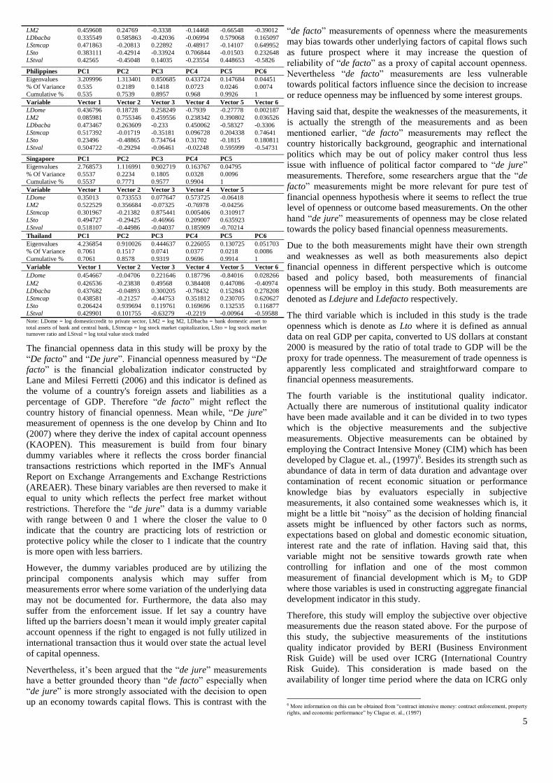
long run cointegration may not be detected. Therefore, prior to

cointegration test a unit root test is essential in order to avoid

such problems and Augmented Dickey Fuller (ADF) along with

Phillip and Perron (PP) test will be employ. The result is as in

table 3 and 4.

Table3: ADF and PP test at level – I(0)

Variables Augmented Dickey Fuller (ADF)

Indonesia Malaysia Philippines Singapore Thailand

Lvol -2.28527 -3.15262 -2.14247 -2.30734 -2.01359

Lfd -1.57466 -1.34256 -2.16811 -2.3935 -2.52508

Ldejure -2.34923 -1.66628 -2.72008 -1.53723 -

Ldefacto -2.1445 -3.81441** -1.46612 -2.04718 -2.5461

Lto -3.60794** -1.3969 -0.02801 -2.77342 -2.56916

Lberi -1.99465 -4.07997** -2.90527 -2.357 -1.44104

Lex -2.35555 -2.54417 -0.43979 -3.16884 -1.19917

Lgovex -2.23115 -1.68713 -2.56508 -2.10582 -2.24478

Lincpc -1.19669 -2.51092 -1.96463 -1.13087 -2.00501

Linf -4.71221*** -3.95455** -6.05135*** -4.74724*** -4.63075***

Lint -2.71115 -2.77918 -2.76329 -3.42105* -3.67186**

Variables Philip and Perron (PP)

Indonesia Malaysia Philippines Singapore Thailand

Lvol -2.59624 -2.5401 -2.47118 -2.48863 -2.61795

Lfd -1.57466 -1.22689 -2.29742 -2.4204 -1.85492

Ldejure -2.21487 -1.08006 -2.74688 -1.53723 -

Ldefacto -2.17042 -3.81441** -1.40117 -2.22978 -2.5061

Lto -3.51358* -0.80461 -0.15002 -2.37239 -2.66821

Lberi -1.99465 -4.51312*** -3.80175** -2.43786 -1.47206

Lex -2.4238 -2.20817 -0.97397 -2.20887 -1.4884

Lgovex -1.94083 -1.84332 -2.80955 -2.10582 -1.64334

Lincpc -1.29061 -2.30131 -1.79413 -1.16165 -1.66903

Linf -4.58039*** -3.89111** -6.49581*** -4.58254*** -4.60334***

Lint -2.82227 -2.58444 -2.09096 -2.60335 -2.88976

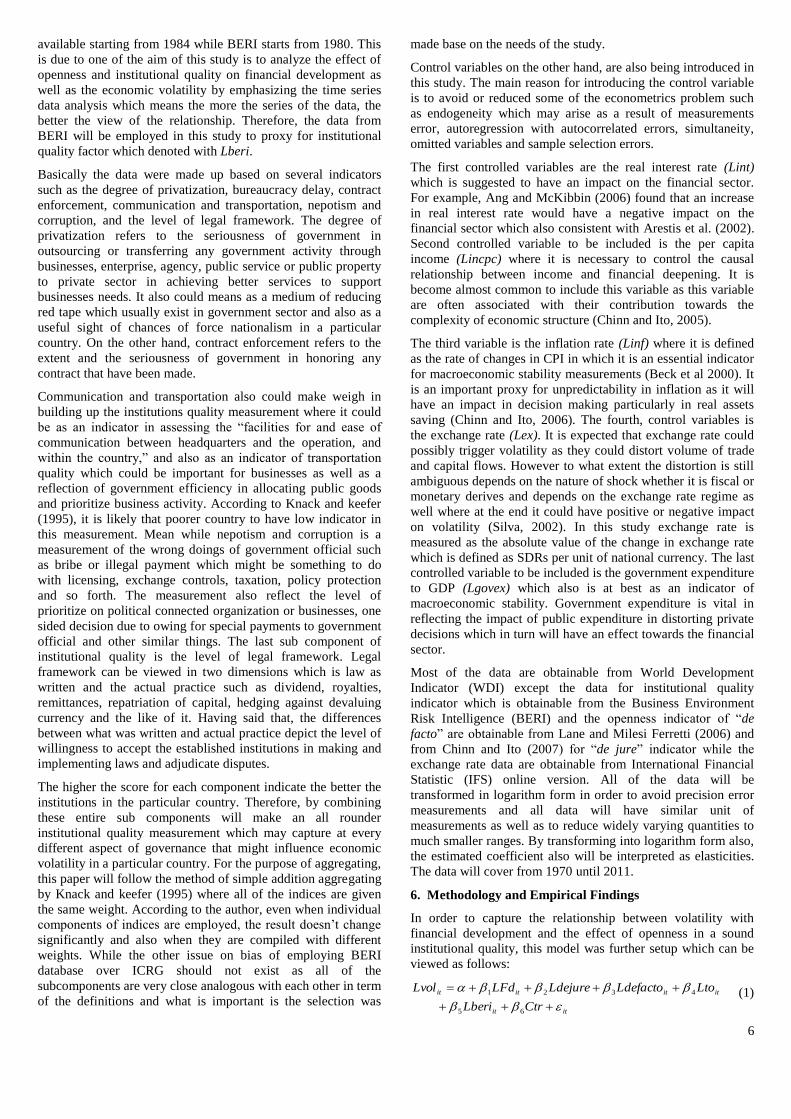
Note: *, ** and *** indicate significance level at 10%, 5% and 1%

Table 4: ADF and PP test at 1st difference – I(1)

Variables Augmented Dickey Fuller (ADF)

Indonesia Malaysia Philippines Singapore Thailand

Lvol -5.55784*** -4.46507*** -6.41748*** -5.02257*** -3.67015**

Lfd -5.52675*** -5.9065*** -6.93325*** -5.4623*** -4.31074***

Ldejure -8.59547*** -4.66648*** -6.86955*** -4.66728*** -

Ldefacto -6.80268*** -6.14235*** -7.06358*** -5.60834*** -7.22065***

Lto -8.30516*** -5.10467*** -5.37681*** -5.82823*** -6.76839***

Lberi -6.40976*** -6.21031*** -4.00312** -5.53684*** -5.54748***

Lex -6.65154*** -4.93398*** -4.84474*** -3.90273** -5.19287***

Lgovex -7.58525*** -6.16589*** -5.41127*** -5.19302*** -5.23091***

Lincpc -5.39917*** -5.04941*** -4.28522*** -5.15183*** -4.48715***

Linf -8.7251*** -7.03688*** -8.36367*** -6.69856*** -7.77897***

7 There is a possibilities of mix level of stationarity in this study as such variables as inflation rate, interest

rate and financial openness indicator are all may subject to rapid intervention of government as a tool of

monetary policy and international policy 8 This study contains variables with 30 to 40 years of observation thus employing ARDL method seems

imminent.

Lint -6.13653*** -6.50074*** -5.79677*** -5.08477*** -4.76334***

Variables Philip and Perron (PP)

Indonesia Malaysia Philippines Singapore Thailand

Lvol -6.10007*** -4.46507*** -6.51351*** -5.02185*** -3.70417**

Lfd -5.44523*** -6.15592*** -6.93203*** -7.50976*** -4.07549**

Ldejure -8.65081*** -3.89959** -6.87036*** -5.74458*** -

Ldefacto -6.80649*** -10.9251*** -7.47337*** -5.61356*** -7.44433***

Lto -8.6608*** -5.07113*** -5.3687*** -5.82233*** -6.76937***

Lberi -6.34989*** -29.314*** -3.96656** -5.61086*** -6.07186***

Lex -6.69909*** -4.78617*** -4.83897*** -3.51264* -5.2139***

Lgovex -7.49917*** -6.16988*** -5.52937*** -5.14546*** -5.3666***

Lincpc -5.39917*** -5.00529*** -4.27414*** -4.67511*** 0.7464***

Linf -10.1573*** -8.27553*** -20.3093*** -17.4313*** -8.91351***

Lint -7.39224*** -11.263*** -14.4609*** -6.41287*** -5.23729***

Note: *, ** and *** indicate significance level at 10%, 5% and 1%

From the table, it shows that only few of regressors variables

exhibit I(0) stationarity while the regressand and all of other

variables cannot reject the presence of unit root at level.

However, after conducting the unit root test in first difference

the result shows that all of the variables have become stationary

at first difference and most of them significant at 1%

significance level I(1).

In other related issue, it is also observed that the unit root test

for financial openness measured by dejure was not included in

the test for Thailand. This is because the data show no variation

in the trend between 1970 until 2004 which made any

regression with the variable seems impossible and also raises

the doubt over the data reliability for Thailand where it is well

known that Thailand took an important step in lifting up the

barrier on its capital account, FDI restrictions and foreign

borrowing in late 80’s until before the 1997 crisis9. Due to this

situation, the variable needs to be taken out from the model for

Thailand.

After understanding the underlying background of each

variables data and under this circumstance especially when

facing with mix stationariy variables, by employing the ARDL

bound test for cointegration would be the most efficient way in

determining the long run relationship among the variables

moreover in small sample dataset. However, prior to the

procedure, the underlying order of auto regression (AR) need to

be estimate as one of the important issues of ARDL

cointegration test is the lag length determination where

randomly choosing the lag length may lead towards inefficiency

or biased estimates parameter. In determining the order of AR,

Aikake’s Information Criteria (AIC) is preferred rather than the

Schwarz Bayesian Criteria (SBC)10

. The lag length criteria, the

list of variables and the number of optimum lag length criteria is

presented in the appendix section of 1A.

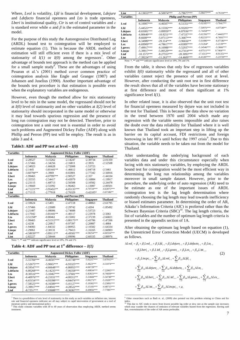
After obtaining the optimum lag length based on equation (1),

the Unrestricted Error Correction Model (UECM) is developed

as follows.

t

x

i

y

i

itiiti

v

i

w

i

itiiti

u

i

iti

t

i

iti

q

i

r

i

s

i

itiitiiti

p

i

ti

o

i

itit

ttttt

tttttt

LincpcL

LexLgovexLLberi

LtoLdefactoLdejure

LfdLvolLincpc

LLexLgovexLLberi

LtoLdefactoLdejureLfdLvolLvol

0 0

2120

0 0

1918

0

17

0

16

0 0 0

151413

1

113

1

12111

11019181716

15141312110

int

inf

intinf

(2)

9 Other researchers such as Badi et. al., (2009) also pointed out this problem relating to Chinn and Ito

index. 10 This due to AIC tends to move from lowest possible lag order at slow rate as the sample size increases

which may wander the chances of omission of relevant variables biased from the regression. Having said

that, overestimation of the order of AR seems preferable.

8

As usual the β is the estimated coefficient, Δ is the difference

operator and µ is the white noise disturbance term. From the

UECM, the long run elasticities can be obtained from the

independent variable coefficient of the first lag divided by the

dependent variable coefficient of the first lag. In conducting the

ARDL bound test, it involve several step where the first step is

to estimate equation (2) by using the Ordinary Least Square

(OLS) technique then proceeded with the calculation of F-

statistic (Wald test) to determined the existence of long run

relationship between aggregate economic volatility and its

determinants. The Wald test is done by imposing a restriction

on both dependent and independent variables coefficients where

the null and alternative hypothesis of equation (2) can be view

as following.

H0 : β1 = 0 …...βi = 0 (No long run relationship)

H1 : β1 ≠ 0 …...βi ≠ 0 (Exist long run relationship)

Then, the estimated Wald test F stat is compared with the

critical values provided by Paseran et. al. (2001) and Narayan

(2005). If the calculated F stat is lower than the critical values

than the null hypothesis of no cointegration will not be rejected

where it assume that the regressors are cointegrated of order

zero I(0). On the other hand, if the calculated F stat exceed the

upper critical value than the null hypothesis of no cointegration

can be rejected where it assume that the regressors are

cointegrated at order one I(1). However, if the calculated F stat

falls between the lower and upper bound, then no conclusion

can be made.

The results of ARDL couintegration based on equation (2) are

as follows.

Table 5: Long run coefficients of the UECM results based

on equation (2)

I. Estimated Model

Variable Indonesia Malaysia Philippines Singapore Thailand

Constant 16.28770

(1.303177)

-46.68303

(-0.655644)

-23.61783***

(-4.212776)

-102.7617*

(-2.538747)

-116.4875**

(-2.976877)

Lvol t-1 -2.501958***

(-7.669844)

-0.865959**

(-2.579258)

-0.971475***

(-3.529380)

-0.608958**

(-3.768341)

-0.708897*

(-1.896355)

Lfd t-1 -0.954951**

(-3.330524)

-2.841308

(-1.979420)

0.750217*

(1.947015)

-1.237306*

(-2.565102)

-7.343235**

(-2.307098)

Ldejure t-1 -1.535116

(-0.394802)

-3.009972**

(-3.036930)

-0.895013**

(-2.944416)

2.478401**

(3.362056)

Ldefactot-1 6.636988***

(5.847089)

-1.148548

(-0.666615)

2.427616**

(3.105067)

1.986597***

(4.074617)

-1.199344

(-0.677330)

Lto t-1 18.35930***

(5.392568)

-14.77133***

(-4.909498)

-1.767194**

(-2.333654)

-2.953602*

(-2.307630)

-8.373137**

(-3.069667)

Lberi t-1 11.80365*

(2.319463)

-4.198213

(-0.264818)

4.259750**

(2.911652)

24.91888**

(2.626151)

11.81651

(1.478062)

Linf t-1 -5.119772**

(-3.424439)

-0.686878

(-1.527405)

0.740029*

(2.205309)

Lgovex t-1 13.52572**

(3.040839)

-16.21248**

(-3.458740)

Lex t-1 -2.376610**

(-3.593044)

-3.479213*

(-2.031231)

7.282700**

(2.395190)

Lint t-1 3.593907***

(5.863104)

1.194607**

(2.644559)

-0.531025

(-1.690097)

Lincpc t-1

6.053503**

(2.616684)

9.648564**

(2.862000)

II. Goodness of fit

R2 0.978044 0.957668 0.848506 0.950942 0.901766

Adj R2 0.840817 0.771407 0.528687 0.735089 0.643903

Std error 0.211767 0.329371 0.206152 0.113458 0.357317

F-Statistic 7.127206** 5.141534** 2.653076* 4.405495* 3.497067**

AIC -0.548228 0.536826 -0.111169 -1.594675 0.924525

III. Diagnostic checking

Normality

test

0.641970

[0.725434]

4.192683

[0.122905]

0.448969

[0.798928]

1.340146

[0.511671]

0.213577

[0.898716]

Serial

correlation

2558.877***

[0.0004]

5.261774

[0.1638]

4.494374

[0.3503]

3.545274

[0.2278]

3.013701

[0.1964]

ARCH

test

1.743601

[0.1732]

1.779339

[0.1819]

0.886418

[0.4899]

0.757633

[0.5304]

0.857392

[0.4771]

RESET

test

4.103269

[0.3446]

3.384173

[0.2364]

1.073603

[0.3920]

0.716366

[0.6272]

1.784380

[0.2465]

Note: *, ** and *** indicate the significant level at 10%, 5% and 1% respectively. Figure in the square

brackets [] quoted the probability values and figure in round bracket () indicate the t test value.

The results indicate that the goodness of fit measurements of the

model remain superior for all of the countries under observation

especially the reported value of R2, adjusted R

2 and the standard

error. The F stat also indicates that there is a significant

relationship among the variables at 10% and 5%. In sum, all of

the variables fit the model well for the entire set of country

under observation.

On the other hand the diagnostic checking indicate that the

model have been correctly specified under the RESET test for

all of the country under observation. The model also has passed

the normality test measured by the Jarque Bera test where both

level of skewness and kurtosis have been checked while the

ARCH test checked for the presence of heteroscedasticity in the

model and none have been detected. However, under the serial

correlation test which is reported by the Breusch Godfrey LM

test indicate that there is a possibility of the serial correlation

between the error term and the specified model in case of

Indonesia. Moreover, the reported CUSUM test also shows that

the series has exceeded the minimum bound for Indonesia

which shows that the model might suffer from instability of

long run coefficients issue11

. Therefore, any results

interpretation regarding Indonesia has to be carried out properly

as there is some issues with the diagnostic checking as noted.

Nevertheless for the rest of the country under observation, there

has been no issue with the diagnostic checking test and they

have passed those tests easily thus any interpretation out of it

can be considered as reliable as reported in table 5.

Table 6 summarize the long run relationship based on equation

(2) where the computed F stat are generated using the Wald test

which then will be compared with the asymptotic critical values

generated by Paseran et. al. (2001) and Narayan (2005) for

specific sample size.

Table 6: Results of the ARDL bounds test

Country Computed F-statistic

Indonesia 10.30195**

Malaysia 7.121457**

Philippines 5.125420**

Singapore 6.791438**

Thailand 4.176731**

Unrestricted

intercept and no

trend

Critical values

(Table CI(iii) case III – Paseran et al. (2001)

Significance level Lower

bound

Upper

bound

Lower

bound

Upper

bound

Lower

bound

Upper

bound

(k = 7) (k=8) (k=9)

1% 2.96 4.26 2.79 4.1 2.65 3.97

5% 2.32 3.5 2.22 3.39 2.14 3.3

10% 2.03 3.13 1.95 3.06 1.88 2.99

Note: *,** and *** indicate significant level at 10%, 5% and 1% based on Wald test. Number in bracket ()

indicate the value of degree of freedom while the critical value table is obtained based on paseran et. al.,

(2001) and Narayan (2005) unrestricted intercept and no trend table CI(iii) case III.

The calculated F stats for Malaysia, Philippines, Singapore and

Thailand exceed the upper critical value at 7 degree of freedom

and Indonesia at 9 degree of freedom which indicates that the

null hypothesis of no cointegration among the observed

variables can be rejected at least at 5% for all cases. Therefore,

it can be concluded that there is a consistent long run

relationship between volatility, financial development, openness

and institutional quality in ASEAN 5 countries.

Table 7 shows the long run elasticities and short run causality

for ASEAN 5 countries of all of the regressors.

Table 7: Short run causality and long run elasticities

I. Long run estimated coefficient

Variable Indonesia Malaysia Philippines Singapore Thailand

Lfd -0.38168** -3.28111 0.772245* -2.03184* -10.3587**

Ldejure -0.61357 -3.47588** -0.92129** 4.069905**

Ldefacto 2.652718*** -1.32633 2.498897** 3.262289*** -1.69185

11 A graphical presentation of the CUSUM test is reported in appendix 1A.

9

Lto 7.337973*** -17.0578*** -1.81908** -4.85026* -11.8115**

Lberi 4.717765* -4.84805 4.384827** 40.92052** 16.66887

Linf -2.04631** -0.70705 1.21523*

Lgovex 5.406054** -18.722**

Lex -0.9499** -5.71339* 10.27328**

Lint 1.436438*** 1.229684** -0.74909

Lincpc 6.990519** 13.61067**

II. Short run causality test (Wald test/ F-statistic)

Variable Indonesia Malaysia Philippines Singapore Thailand

∆Lfd 32.68050*** 2.362106 4.069613* 3.067862 1.145910

∆Ldejure 17.88078** 0.706129 4.239442* 8.777534**

∆Ldefacto 0.103051 0.194406 3.688662* 0.021089 0.170328

∆Lto 28.16926*** 16.46085*** 2.545739 3.324536 8.132005**

∆Lberi 7.800459** 0.665836 0.484104 6.359163** 0.402449

∆Linf 10.94070** 0.525235 3.067650

∆Lgovex 11.09668** 3.020265

∆Lex 5.062615* 0.389797 1.680050

∆Lint 3.909624 3.401333* 0.015732

∆ Incpc 6.386439* 4.144343*

Note: *, ** and *** indicate the significant level at 10%, 5% and 1% respectively. The ∆ operator indicate the first difference operator.

From the reported table, it is clear that financial development

(Lfd) is significant and negative in the cases of Indonesia,

Singapore and Thailand as expected while positive in

Philippines. This imply that the aggregate economic volatility

falls by 0.38% in Indonesia, 2.03% in Singapore and 10.36% in

Thailand when there is a 1% increase in aggregate financial

development while in Philippines an increase in aggregate

financial development may rise aggregate economic volatility

by 0.77%. This suggest that financial development are able to

reduce economic volatility in long run by means of international

risk sharing and efficient fund management as already known

that those countries have taken an important step in

restructuring their financial sector 1980’s followed by another

significant reform in the aftermath of 1997 financial crisis such

as establishing appropriate institutional frameworks,

abolishment of nonviable financial institutions from the system

and strengthening viable institutions through consolidation,

recuperating regulations and supervision in banking sector as

well as promoting transparency in financial market operations.

However, different case for Philippines even though after series

of financial reform but still fail to establish financial sector

development as a mean for mitigating economic volatility. One

possible explanation for this might be inadequate financial

policy measurements which then followed by weak institutional

quality where it is well known that Philippines have been listed

among the most corrupted country which also have reported

under the Business Environment Risk Intelligence (BERI) and

International Country Risk Guide (ICRG) where the score of

institutional quality was low at about 3 out of possible 100 from

1980 until 2011 and 2.2 out of possible 100 from 1984 until

2008 respectively. It is also well known that the country has saw

the assassination of their top leader previously which indicate

that the level of institutional quality in Philippines is low where

all this factor might explain the insignificant of financial sector

development measurements in Philippines. Hence this situation

might have led towards more volatile state of economy and

measurement of financial development had become a

contribution towards economic fluctuation on longer term in

case of Philippines.

The financial openness (Ldejure) indicates that it is a significant

determinant in Malaysia, Philippines and Singapore. In

Malaysia and Philippines shows that any policies regarding

capital account openness have succeed in reducing volatility by

3.5% and 0.9% in long run while in Singapore financial

openness policy may trigger volatility by 4.1%. This shows that

openness measured by policy (de jure) are able to reduce

volatility in Malaysia and Philippines where it might have create

better risk sharing and well diversified investment portfolio

which could be vital in reducing the impact of economic shocks

as well as by permitting the presence of more foreign bank will

increase the domestic banking system efficiency. For instance,

Chiang Mai initiative took place in the aftermath of 1997 crisis

might have help contributing towards lowering volatility as well

as an ASEAN Comprehensive Investment Agreement (ACIA)

which was later on signed in February 2009 which main

objectives were to create a free and open investment regime

thus realizing economic integration. The ACIA streamlines the

existing ASEAN investment agreements, with a view to

attracting more foreign investment into ASEAN and increasing

intra-ASEAN investment. However, in Singapore any in

changes in financial openness policy may trigger their economic

volatility which might be due to the fact that Singapore is the

third largest financial centre in Asia after Japan and Hong Kong

as well as Singapore has become a financial instruments trading

hub for ASEAN countries. Therefore, a small open economy of

Singapore economic activity depends much on international

financial trading which make their economic activity level more

sensitive towards the changes on financial openness policy.

However in term of outcome of the financial openness policies

(Ldefacto), it indicates that it may have a positive significant

effect in triggering more volatility in long run in case of

Indonesia by 2.7%, 2.5% in Philippines and 3.3% in Singapore.

This shows that the outcome of rising financial openness may

only trigger more economic volatility in all cases as openness

may increase financial activity level moreover in profit taking

activity by investors as well as increasing the volume of

financial instrument turnover. This shows the cyclical nature of

capital flows where large sum of fund coming in into an

economy will then followed by capital outflows. This was

parallel with Singapore where the aggregate economic volatility

have risen by 33% from 1976 until 2011 along with financial

openness (ldefacto) which have grow more than 7 times since

1970 which match with the role of Singapore as a financial hub

especially in ASEAN region. In the case of Philippines and

Indonesia, the positive relation between financial openness

(Ldefacto) and aggregate volatility (Lvol) is due to the fact that

both country level of openness have sharply decrease since the

1997 East Asia financial crisis by 82% in Philippines and 78%

in Indonesia since 1997 crisis due to more careful step by

investor in investing especially in Indonesia and Philippines and

it is also one of the measurements taken in order to calm down

their economic volatility by both country. Therefore, in

Indonesia economic volatility has reduced as much as 26% and

20% respectively since 1997 and this result was parallel with

recent economic occurrences.

On the other hand, trade openness (Lto) also is a significant

determinant on economic volatility for all of ASEAN 5

countries in long run. It demonstrates that there is a negative

relationship between trade openness and volatility except in the

case of Indonesia. As for Malaysia it shows that an increase in

trade openness is able to reduce economic volatility as large as

17.1%, 1.8% in Philippines 4.9% in Singapore and 11.9% in

Thailand. This shows that trade openness may deviate escalating

inflation which may trigger volatility by substitution effects as

well as increase in product specialization where by specializing

may reduce the cost of product in long term thus eliminating the

chances of excessive volatility driven by inflation. In other

words, openness in trade segment may improve resource

allocation, lowers consumers’ prices and leads towards more

efficient production thus reducing volatility. Moreover it also

10

encourages the technological transfer which may result in

productivity improvements thus increasing economic

development which could mean a reduced impact on volatility.

This is in line with increasing number of bilateral trade

arrangements especially among ASEAN countries and with

other country such as Australia under the free trade agreement

with Australia and New Zealand (AANZFTA) on August 2008

which is expected to favor both regions investment in term of

trade and finance. However, in Indonesia an increase in trade

openness is estimated to increase economic volatility by 7.3%.

As already know that Indonesia is among most affected country

hit by the 1997 crisis which have affected their trade industries

and saw a sharp decrease in trade activities as much as 11% due

to the crisis. It is suggested that the Indonesian government to

increase their reserves during the favorable swing which then

can be used when the event of bad volatility set in to smoothen

out the impact on trade sector.

Institutional quality (Lberi) is found to be positive significant

determinants in Indonesia, Philippines and Singapore. From the

analysis, it shows that by strengthening institutional quality it

may have increase the level of economic volatility by 4.7% in

Indonesia, 4.4% in Philippines and 41% in Singapore in long

run. This result was surprisingly contradict with the early

hypothesis which by strengthening institutional quality should

have a reduce impact on volatility. Among possible explanation

for this situation is might due to by strengthening institutional

quality might encourage streaming of economic resources

towards political linkages institution including towards

incompetent institutions which in turn may drag their economy

towards volatile state of economy especially in the case of

Indonesia and Philippines as both of them are among countries

which always associate with political instability. However, in

case of Singapore this explanation might not be applied as they

are among less corrupted economy and one possible explanation

is sometimes by rapid changes in upgrading institutional quality

especially the set of legal framework might not be favorable by

some investors thus affecting the flow of capital inwards and

outwards the country hence triggering more volatility especially

when Singapore itself is one of the most active country involved

in international trade and finance.

The set of control variables also show a significant relationship

in those countries which reflect important role of fiscal and

monetary policy as well as income factor. Fiscal policy is

reflected by government expenditure (Lgovex) and it is

negatively significant in Malaysia and positive in Indonesia

which means that fiscal policy in Malaysia are able to control

excessive volatility by 18.7% while in Indonesia their fiscal

policy have led towards more volatility as much as 5.4% in long

run. On the other hand, monetary policy indicators such as

inflation (Linf) in Singapore act as a contributing factor towards

volatile state by 1.2% and the decreasing level of inflation in

Indonesia are able to reduce volatility by 2% in longer term.

Exchange rate (Lex) policy on the other hand seems to reduce

volatility in Indonesia by 0.9% and Singapore by 5.7% which

shows effective monetary policy in attracting more foreign

funds inwards the country with less capital flight. However in

Thailand, the effect of Asian financial crisis on their exchange

rate have given massive impact where the results reveal that

exchange rate have added towards more volatility by 10% in

long run. Interest rate (Lint) in Indonesia and Philippines seems

to have positive impact as much as 1.4% and 1.2% respectively

which shows that rapid intervention in monetary policy in long

run may trigger more volatility as much of investments decision

depends on the level of interest rate. Mean while, income per

capita (Lincpc) shows that it is a positive significant

contribution towards volatility in Malaysia and Thailand as

much as 7% and 13.6% respectively. This shows that an

increase in income per capita trigger more volatility in both

country in long run as more international transaction taking

place which might due to preference of international products

and investment abroad.

On the other hand, the short run causality shows that aggregate

financial development indicator (Lfd) is positive significant

indicator in Indonesia and Philippines. The financial openness

indicator measured by de jure also indicates that it is a positive

significant in Indonesia, Philippines and Singapore while de

facto only significant in Philippines. On the other hand trade

openness (Lto) is significant in Indonesia, Malaysia and

Thailand while institutional quality (Lberi) is significant

determinant only in Indonesia and Singapore. Mean while the

set of control variables such as inflation rate (Linf), government

expenditure (Lgovex) and exchange rate (Lex) only significant

in Indonesia while interest rate (Lint) is significant determinant

is Philippines only. The effect of income per capita (Lincpc) is

affecting volatility only in Malaysia and Thailand in short run.

As a sum all of the short run causality is positive related

towards volatility which shows that any small changes could

lead towards triggering economic volatility in short run as

investors and savers have become more skeptical about ASEAN

5 market moreover after the 1997 East Asia financial crisis

lesson.

7. Conclusion

In sum, this paper examines the existence of cointegration

relationship between the aggregate economic volatility and

financial development, simultaneous openness in both financial

and trade segment as well as the quality of institutions in

ASEAN 5 economies namely Indonesia, Malaysia, Philippines,

Singapore and Thailand during the period of 1970 until 2011. In

achieving the conclusion, ARDL bound test developed by

Paseran et. al., (2001) were utilized and the empirical results

reveal the existence of long run relationship between aggregate

economic volatility and its determinants in ASEAN 5

economies. However, there is a model stability issue in case of

Indonesia where any interpretation of the results need to be

carried out properly and with cautious.

Among the vital information reveal from the analysis is that the

aggregate financial development is a significant and negatively

related to economic volatility in Indonesia, Singapore and

Thailand while positive in Philippines. In other words,

aggregate financial development is able to reduce aggregate

economic volatility except in Philippines where it will lead to

more economic volatility. Therefore, aggregate financial

development will lead towards less volatility in most cases in

ASEAN 5 economies. However, in reviewing the Europe and

US financial crisis, some have point out that the use of complex

currency as well as credit derivatives structures are among the

contributor towards the crisis which means that as financial

sector getting develop, the more complexness of financial

structure will be become. Having said that, ASEAN 5 countries

have to learn from the Euro zone conflict and become more

cautious or otherwise the reducing effect of financial

development on economic volatility will vanish. Such effort as

the ASEAN Comprehensive Investment Agreement (ACIA) and

Chiang Mai initiative are all proven to be crucial and it is

suggested that more agreements which may benefit financial

11

development should be initiated.

On the other hand, both type of openness which is financial and

trade are also considered to have a significant impact on

economic volatility. Financial openness provides a mix

conclusion where it depends on the type of measurements. If it

is measured from the policy (de jure) effect point of view, it

seems that it may have a reduce impact on volatility in most

cases. Among other researchers who come with similar

conclusion is Bekaert et al (2006) where they demonstrate that

countries with more open capital account tend to reduce

consumption growth volatility moreover after equity market

opening and financial opening also tend to reduce the ratio of

consumption growth volatility to GDP growth to volatility due

to improved risk sharing. However, if it is from the financial

openness outcome (de facto) view, then financial openness may

lead towards more volatile state of economy which is parallel

with the finding such as Buch et al., (2005) which suggest that

the link between financial openness and volatility has not been

stable over time which could only trigger crises. Therefore,

financial liberalization, if carried out inappropriately, may

encourage destabilization in the financial system and trigger

financial crises (Ang and McKibbin, 2006). Having said that, if

financial openness is view from “de facto” perspective, then the

IMF hypothesis does not hold and this may be the answer of

rapid economic development in China and India.

Trade openness on the other hand is significant and negatively

related in most of ASEAN 5 countries except for Indonesia

where trade openness has been a means in relaxing economic

volatility in most of ASEAN 5 countries which also indicate the

success of ASEAN Free Trade Agreements (AFTA) in

increasing economic integration. According to Razin and Rose

(1992), trade openness may encourage specialization thus

increasing the trade volume and with increased specialization of

intra industry would lead towards a declining in output volatility

due to greater volume of intermediate inputs trade.

However, this finding also is contradicted with Kose et. al.,

(2006) where they observed that only trade openness is

significantly positive towards volatility but less robust on

financial openness. However, the sample is based on 92 cross

country analysis while this study is based on time series analysis

for every single country. Some researchers might argue that

definitely for economic policies, diversity in historical

experiences and institutional factors are equally important as

well as the cultural norms contexts which is difficult to interpret

with cross country analysis (Hasan et, al., (2007) and this might

explain the differences in the results as well as some difference

variables involve. On the other hand, it is also suggested that

any empirical analysis should weight financial and trade

openness simultaneously in the same model as been suggested

by IMF (2003) and Rajan and Zingales (2003) where financial

and trade openness should go hand by hand as the two sector

barely need each other in other in order to developed and also in

real world the interdependent among the two is very high.

Institutional quality also proven to be a positive significant

effect in this study for Indonesia, Philippines and Singapore

while in the other countries, institutional quality has no

significant impact. However the effect of institutional quality is

not consistent with other researchers finding and is contradict

with most of other findings. Among of possible theoretical

explanation is strong institutional quality often relates with

absolute control of power where absolute control might leads

towards misused of power and less debate or arguments of

policy. For instance, they could misuse the powers for political

benefit or even personal benefit. This in turn may reduce the

welfare and economic maximization thus triggering capital

flight and encourages volatility. As a fact which already known

that both Indonesia and Philippines have experienced to live

with this circumstances under the Suharto and Sukarno regime

in Indonesia and Fidel Ramos in Philippines which they always

associated with controversy or could also due to paradox of

enrichment or it could also due to reverse causality effect. This

means that whenever the country confronted with excessive

volatility, they tend to strengthen their institutional quality in

order to overcome the situation by attracting more investments

to balance the gap. The reverse causality possibilities between

institutional quality and volatility are up for further future

research.

The other control variables also prove to be a significant

determinant of economic volatility such as fiscal and monetary

policy where this kind of policy should go along together with

liberalization as well as financial sector deepening.

8. REFERENCES 1. Abdullah D. Ahmed and Sandy Suardi, 2009. Macroeconomic Volatility,

Trade and Financial Liberalization in Africa. World Development Vol.

37, No. 10, pp. 1623–1636, 2009. doi:10.1016/j.worlddev.2009.03.009

2. Acemoglu, D., Zilibotti, F. 1997. Was Prometheus unbound by chance? Risk, diversification, and growth, Journal of Political Economy 105, 709-

775.

3. Aghion, P., Bachetta, P., & Banerjee, A. (2004). Capital markets and the instability of open economies. Journal of Monetary Economics, 51(6),

1077–1106.

4. Arestis, P., Demetriades, P.O., Fattouh, B., Mouratidis, K., 2002. The impact of financial liberalization policies on financial development:

evidence from developing economies. International Journal of Finance

and Economics 7, 109–121. 5. Arora, V. and Vamvakidis, A., 2004. How much do trading partners

matter for economic growth? IMF Working Paper No. 04/26.

6. Badi H. Baltagi, Panicos O. Demetriades, Siong Hook Law, 2009. Financial development and openness: Evidence from panel data. Journal

of Development Economics 89 (2009) 285–296

7. Beck, T., Levine, R., 2004. Stock Markets, Banks, And Growth: Panel Evidence. Journal Of Banking And Finance 28, 423–442.

8. Beck, T., Levine, R., Loayza, N., 2000. Finance And The Sources Of

Growth. Journal Of Financial Economics 58, 261–300. 9. Blankenau, W., Kose, M.A., Yi, K., 2001. Can world real interest rates

explain business cycles in a small open economy? Journal of Economic

Dynamics and Control 25, 867–889. 10. Caprio, G., Laeven, L., Levine, R., 2004. Governance And Bank

Valuation. Mimeo. University Of Minnesota

11. Chinn, M., & Ito, H. (2005). What matters for financial development? Capital controls, institutions, and interactions. NBER Working Paper No.

11370. National Bureau of Economic Research, Cambridge.

12. Chinn, M.D., Ito, H., 2006. What matters for financial development? Capital controls, institutions and interactions. J. Dev. Econ. 81, 163–192.

13. Claessens, S., Djanky, S., Fan, J., Lang, L., 2002a. Expropriation of

minority shareholders in East Asia. Journal of Finance 57. 14. Clague, C., Keefer, P., & Knack, s., (1997). Contract-Intensive Money:

Contract Enforcement, Property Rights, and Economic Performance,

Journal of Economic Growth, 4: 185–211 15. Claudia M. Buch, Joerg Doepke & Christian Pierdzioch (2005). Financial

openness and business cycle volatility. Journal of International Money

and Finance 24 744-765

16. Geert Bekaert, Campbell R. Harvey, Christian Lundblad, 2006. Growth

volatility and financial liberalization. Journal of International Money and Finance 25, 370 - 403

17. Gisele Ferreira da Silva, 2002. The impact of financial system

development on business cycles volatility: cross-country evidence. Journal of Macroeconomics 24, 233–253

18. Iftekhar Hasan, Paul Wachtel, Mingming Zhou, 2009. Institutional

Development, Financial Deepening and Economic Growth: Evidence From China. Journal of Banking & Finance 33, 157–170

19. James B. Ang, Warwick J. Mckibbin, 2006. Financial Liberalization,

Financial Sector Development and Growth: Evidence From Malaysia. Journal of Development Economics 84 (2007) 215–233

20. Johnson, S., Mcmillan, J., Woodruff, C.M., 2002. Property Rights And

Finance. American Econ. Rev. 92, 1335–1356.

12

21. Kalemli-Ozcan, S., Sorensen, B.E., Yosha, O., 2003. Risk sharing and

industrial specialization: regional and international evidence. American

Economic Review 93, 903–918 (June). 22. Kim, D.-H., et al., 2009. Dynamic effects of trade openness on financial

development, Economic Modelling, doi:10.1016/j.econmod, .09.005

23. Kiyotaki, N. and Moore, J. 1997. Credit Cycles, Journal of Political Economy 105, 211- 48.

24. Knack, S., Keefer, P., 1995. Institutions and economic performance:

cross-country tests using alternative institutional measures. Econ. Polit. 207–227.

25. La Porta, R., Lopez-De-Silanes, F., Shleifer, A., Vishny, R.W., 1997.

Legal Determinants Of External Finance. Journal Of Finance 52, 1131–1150.

26. Lane, P.R., Milesi-Ferretti, G.M., 2006. The external wealth of nations Mark II: revised and extended estimates of foreign assets and liabilities

1970–2004. IMF Working Paper 06/69.

27. Levine, R., 2001. International financial liberalization and economic growth. Rev. Int'l. Econ. 9, 688–702.

28. Levine, R., 2005. Finance and growth: theory and evidence. In: Aghion,

P., Durlauf, S. (Eds.), Handbook of Economic Growth. Elsevier, Amsterdam.

29. M. Ayhan Kose, Eswar S. Prasad, Marco E. Terrones, 2006. How do

trade and financial integration affect the relationship between growth and volatility?. Journal of International Economics 69 (2006) 176– 202

30. Menzie D. Chinn and Hiro Ito (2007). A New Measure of Financial

Openness, Journal of Comparative Policy Analysis, Volume 10, Issue 3, p. 309-322.

31. Narayan, P.K., (2005). The saving and investment nexus for China:

Evidence from co-integration tests. Applied Economics, 37, 1979- 1990. 32. Pesaran, M. H., Shin, Y., & Smith, R.J., (2001). Bounds testing

approaches to the analysis of level relationships. Journal of Applied

Econometrics 16(3), 289-326. 33. Pindyck, R. S. (1991). Irreversibility, uncertainty, and investment.

Journal of Economic Literature, 29(3), 1110–1148.

34. Raj Aggarwal, John W. Goodell, 2009. Markets versus institutions in developing countries: National attributes as determinants. Emerging

Markets Review 10 (2009) 51–66

35. Rajan, R.G., Zingales, L., 2003. The Great Reversals: The Politics Of Financial Development In The Twentieth Century. J. Financial Econ.

69,5–50.

36. Razin, A., & Rose, A. K. 1992. Business-cycle volatility and openness. An exploratory cross-sectional analysis. In L. L. Editor, & A. R. Editor

(Eds.), Capital mobility: The impact on consumption, investment, and

growth (pp. 48–76). Cambridge: University Press. 37. Razin, A., Sadka, E., & Coury, T. 2003. Trade openness, investment

instability and terms-of-trade volatility. Journal of International

Economics 61, 285–306

38. Rodrik, D., 1998. Who needs capital-account convertibility? In: Fischer,

S., Cooper, R.N., Dornbusch, R., Garber, P.M., Massad, C., Polak, J.J.,

Rodrik, D., Tarapore, S.S. (Eds.), Should the IMF pursue capital-account convertibility? International Finance Section, Department of Economics,

Princeton University, Princeton, NJ, pp. 55–65.

39. Schmukler, S. 2003. Financial globalization: Gains and pain for developing countries. Washington, DC: World Bank. Unpublished

manuscript.

40. Stiglitz, J.E., 2000. Capital market liberalization, economic growth, and instability. World Development 28, 1075– 1086.

41. Thorsten Beck, Aslı Demirgüç-Kunt and Ross Levine, (2000), "A New

Database on Financial Development and Structure," World Bank Economic Review 14, 597-605. (An earlier version was issued as World

Bank Policy Research Working Paper 2146.)

Appendix 1A

Optimum lag length based on Aikake’s Information Criteria

(AIC)

Variables Indonesia Malaysia Philippines Singapore Thailand

Lvol 1 2 1 1 3

Lfd 1 1 1 3 3

Ldejure 2 3 1 1 -

Ldefacto 1 3 1 1 1

Lto 1 1 1 1 1

Lberi 1 2 2 3 1

Linf 3 1 3 2 1

Lgovex 3 1 1 1 3

Lex 1 2 2 2 1

Lint 1 1 1 3 1

Lincpc 1 1 2 3 2

Graphical report of CUSUM test

Indonesia

Malaysia

Philippines

Singapore

Thailand

-6

-4

-2

0

2

4

6

2008 2009 2010 2011

CUSUM 5% Significance

-8

-6

-4

-2

0

2

4

6

8

2006 2007 2008 2009 2010

CUSUM 5% Significance

-10.0

-7.5

-5.0

-2.5

0.0

2.5

5.0

7.5

10.0

2003 2004 2005 2006 2007 2008 2009 2010 2011

CUSUM 5% Significance

-8

-6

-4

-2

0

2

4

6

8

2007 2008 2009 2010 2011

CUSUM 5% Significance

-10.0

-7.5

-5.0

-2.5

0.0

2.5

5.0

7.5

10.0

2004 2005 2006 2007 2008 2009 2010 2011

CUSUM 5% Significance