Economic Uncertainty and Structural Reforms∗

Alessandra Bonfiglioli† Gino Gancia‡

July 2016

Abstract

Does economic uncertainty promote the implementation of structural reforms? We

answer this question using one of the most exhaustive cross-country panel data set

on reforms in six major areas and measuring economic uncertainty with stock market

volatility. To address endogeneity concerns, we propose various identification strategies,

instrumenting uncertainty with world shocks to volatility and with natural disasters,

political coups and revolutions. Across all specifications, we find that uncertainty has

a positive and significant effect on the adoption of reforms. This result is robust to the

inclusion of a large number of controls, such as political variables, economic variables,

crisis indicators, and a host of country, reform and time fixed effects.

JEL Classification: E02, E60, L51

Keywords: Reforms, Uncertainty.

∗We thank Alberto Alesina, Nicholas Bloom, Jeffry Frieden, Maria Petrova, Giacomo Ponzetto, RomainRanciere, David Strömberg, Guido Tabellini, Aaron Tornell, Fabrizio Zilibotti and seminar participants atUPF, the NBER Summer Institute (Political Economy), the workshop on the Political Economy of TaxReforms (the Hague) and the workshop on the impact of uncertainty shocks on the global economy (UCL)for comments. We acknowledge financial support from the Barcelona GSE and the Spanish Ministry ofEconomy and Competitiveness (ECO2014-55555-P and ECO2014-59805-P).†Universitat Pompeu Fabra, Dept. of Economics and Business, Barcelona GSE and CEPR. Ramon Trias

Fargas, 25-27, 08005, Barcelona, SPAIN. E-mail: alessandra.bonfiglioli@upf.edu‡CREI, Barcelona GSE and CEPR. Ramon Trias Fargas, 25-27, 08005, Barcelona, SPAIN. E-mail:

ggancia@crei.cat

1

1 Introduction

The Great Recession has been accompanied by an enormous increase in macroeconomic

volatility, which has stimulated a new literature on how uncertainty impacts economic activ-

ity and especially investment decisions (e.g., see Bloom, 2009 and 2014). Despite the growing

attention of both economists and policy makers on the topic, little effort has been devoted

to studying the effect of uncertainty on public choices. Such an omission is unfortunate,

because the recent crisis has also exposed the urge for structural reforms. The aim of this

paper is to fill this gap, namely, to investigate empirically the effect of economic uncertainty

on the adoption of structural reforms.

Why governments often fail to adopt reforms even when they are believed to be needed

and welfare-improving is one of the fundamental questions in political economy. For instance,

although most observers tend to agree that promoting product market competition, providing

free access to markets and reducing public debt are often essential to preserve economic

growth, the extent to which such measures are adopted varies enormously across countries.

While the literature has identified several explanations for an anti-reform bias, with many

of them placing distributional conflict as the cornerstone, until now the role of economic

uncertainty has received little attention. As a result, existing theories often lack sharp

predictions.

In some instances, uncertainty can be an obstacle to the adoption of reforms. For example,

uncertainty about the distribution of costs and benefits may lead to a status quo bias (e.g.,

Fernandez and Rodrik, 1991) or to a war of attrition between parties resulting in ineffi cient

delays (Alesina and Drazen, 1991). Other theories suggest that the opposite result may also

hold. For example, more noise can sometimes improve agency problems and this insight

has recently been used by Bonfiglioli and Gancia (2013) to show that economic uncertainty

can alleviate political myopia. The argument is that in times of turmoil reelection depends

more on luck rather than political actions, thereby leaving the government freer to invest in

reforms whose short-run costs are more visible than their future payoffs. On the empirical

side, while there is some evidence that uncertainty discourages private investment, little is

known about its effect on public investment and policy. Although there is some consensus

that reforms are more likely to occur during times of crisis (e.g., Tommasi and Velasco, 1996,

Alesina, Ardagna and Trebbi, 2006, and Ranciere and Tornell, 2015) and that recessions are

associated with higher uncertainty, there is to date no attempt to isolate empirically the

effect of the latter.

In this paper, we use one of the most exhaustive cross-country panel dataset on re-

forms together with recent measures of macroeconomic uncertainty and various identifica-

tion strategies to show that economic uncertainty promotes the implementation of structural

2

reforms. As in Giuliano, Mishra and Spilimbergo (2013), we define a reform as an increase in

deregulation indices available in six areas: domestic financial sector, capital account, product

markets, agriculture, trade, and current account transactions. One advantage of focusing on

these structural reforms is that they are not affected by automatic stabilizers, which react

directly to fluctuations in income. Following a rapidly-expanding literature (e.g., Bloom,

2014), we proxy macroeconomic uncertainty with stock market volatility, built whenever

possible from daily data. The resulting dataset spans 6 reforms in 56 countries with yearly

observations over the period 1973-2006.

As a preliminary step, we show that economic uncertainty is positively and significantly

correlated to the adoption of reforms and that this finding is robust to the inclusion of a

large number of controls such as political variables, economic variables, crisis indicators, and

a host of country, reform and time fixed effects. Moreover, we show that the results do not

depend crucially on any specific subset of the six reform areas, and they are robust to using

more stringent definitions of reforms. Next, we propose several identification strategies to

tackle the issue of the potential endogeneity of our measure of uncertainty. First, to isolate

world shocks that are unlikely to be affected by the adoption of reforms in a single country,

we instrument uncertainty in a given country with average stock market volatility in the

rest of the sample. Second, we follow Baker and Bloom (2013) in using natural disasters,

political coups, revolutions and terrorist attacks as instruments for uncertainty. Finally,

since a concern may still remain that these shocks are not entirely exogenous or may affect

directly policy choices in a given country, we also instrument uncertainty using disasters

and political unrest shocks in the rest of the sample. In all cases, the first-stage regressions

indicate that our instruments are strong predictors of stock market volatility and the over-

identification tests find no evidence to reject them. In all cases, the second-stage results

confirm the initial finding that economic uncertainty, measured by stock market volatility,

promotes the adoption of structural reform.

We close the analysis with some additional robustness checks. In particular, we show our

results to hold if we focus on a country average of the six reforms, if we add further controls

capturing the cycle and economic growth, and if we account for the adoption of reforms

in other countries of the same geographical area. Moreover, the effect of uncertainty is

driven neither by the waves of reforms in EU countries nor by those in Central and Eastern

European Countries. Finally, we investigate further aspects of the relationship between

uncertainty and reforms that can shed more light on the underlying mechanism. First,

we find that the positive effect of uncertainty on the implementation of reforms is weaker

in countries with better quality of information. Second, we show that economic volatility

promotes liberalizations (i.e., a positive change in the deregulation indexes) and not their

reversals (i.e., a negative change in the deregulation indexes). Third, we find that volatility

3

has no effect on social reforms such as the softening of abortion laws. While not conclusive,

these pieces of evidence seem consistent with agency models in which economic shocks mask

the costs of liberalizations.

The remainder of the paper is organized as follows. In section 2 we review the existing

theoretical and empirical literature on reforms and uncertainty. In section 3, we describe

the data and our identification strategies. In section 4, we present the empirical results,

including robustness tests and an investigation of the mechanism. Section 5 concludes.

2 Economic Uncertainty and Reforms: A Look at the Literature

The literature on the political economy of reforms is vast and summarizing it goes beyond

the scope of this section.1 Rather, we briefly discuss some of the main theoretical channels

through which economic uncertainty may affect the incentives to implement reforms and

then review the existing empirical evidence.

2.1 Theory

The term “reform” usually refers to a major change in policy, and common examples of

structural reforms are liberalization of markets for goods or services and changes in the

regulatory environment. Even when considered welfare improving, reforms are often diffi cult

to implement because of the unequal distribution of their costs and benefits. The costs may

arise from relative price changes, implying adjustment costs, transitional unemployment

and redistribution of income between different agents in the society. Frequently, the time

profile is also troubling, with costs being paid up-front and benefits accruing with time (see

Tommasi and Velasco, 1996, for a more extensive discussion). In the absence of effi cient

compensation and incentive schemes, the conflict of interest between winners and loser or

between voters and policy makers can lead to institutional inertia. In such settings, how

does economic uncertainty affect the political viability of reforms? Since existing theories

often do not answer explicitly this question, we now use some of the leading approaches to

discuss possible effects of uncertainty.

There are several reasons why uncertainty may block or delay the adoption of reforms. In

the influential paper by Fernandez and Rodrik (1991), uncertainty regarding the distribution

of gains and losses of a policy change may lead to a status quo bias. Similarly, aggregate

uncertainty about the economic effects of reforms may make gradualism more appealing,

this leading to slow adoption of reforms. Although in these cases uncertainty is about the

consequences of reforms rather than on the state of the economy, it may be diffi cult to

1See Tommasi and Velasco (1996) and Drazen (2000) for some surveys.

4

distinguish the two.

Alesina and Drazen (1991) have instead shown that reforms may be postponed due to a

war of attrition between two groups in the society with veto power. The key assumption is

that each group would like to charge to the other a larger fraction of the adjustment cost,

but is uncertain about the evaluation of this cost by the other group. The passage of time is

needed to reveal who is stronger, since the group with the higher cost of waiting will concede

first. In this model, uncertainty may delay the resolution of the war of attrition, if it regards

the relative strength of the two groups. On the contrary, negative economic shocks, which

could be more likely in turbulent times, may anticipate the reform by increasing the cost of

waiting. Thus, the model predicts that crises, rather than economic volatility per se, can

trigger reforms.2 Finally, Alesina and Cukierman (1990) have shown that uncertainty allows

the politicians to follow their most preferred policy, even at the expenses of voters, and this

may explain why some reforms that would benefit the society at large are not implemented.

The notion that uncertainty can facilitate economic reforms is not commonly found in the

literature. There are however instances in which uncertainty may alleviate agency problems

(e.g., Dewatripont, Jewitt and Tirole, 1999, Holmström, 1999, and Prat, 2005). Building on

this insight, Bonfiglioli and Gancia (2013) show that uncertainty can promote the adoption

of reforms in a model in which elections serve the purpose of selecting the most competent

politicians. As in Rogoff (1990), information frictions prevent citizens from perfectly disen-

tangling the economic effect of competence, reforms and exogenous shocks. The second key

premise is that reforms have short-run costs and future benefits. These assumptions imply

that the costs of reforms are more visible than the benefits thereby inducing an incumbent

politician to underinvest in reforms in an attempt to appear competent and increase his

probability to stay in power. Higher economic uncertainty makes this probability depend

more on luck rather than political actions and hence reduces the myopic, or “opportunistic”,

bias against reforms.

The model formalizes the idea that politician perceive a political cost at implementing

welfare-improving but unpopular reforms. It is also consistent with the observations that

the probability that a government is replaced depends on economic conditions, but not on

reforms.3 It is important to stress that the model does not require reforms to be unobservable,

only the mild assumption that citizens cannot fully separate the true cost of a reform from

2Drazen (2000) discusses other reasons why reforms may be more likely in periods of crisis. See alsoRanciere and Tornell (2015). A recent literature has also shown that (adverse) economic shocks may speedup the transition towards more democratic political regimes (e.g., Acemoglu and Robinson, 2006).

3Since citizens are rational, the equilibrium choice of reform is known. For evidence that reelectionprobability is not negatively affected by reforms see Peltzman (1992), Alesina, Perotti and Tavares (1998),Alesina et al. (2013) and Brender and Drazen (2008).

5

the effect of the competence of the politician undertaking it.4 Yet, since the agency problem

does depend on informational asymmetries, the model predicts the impact of uncertainty

to be stronger if citizens are less informed. We demonstrate these results in the Appendix,

where we present a simplified version of the model.

Economic uncertainty may promote reforms also through other channels. For example,

although we are not aware of explicit formalizations, it is conceivable that aggregate volatility

reduces the support for the status quo. Or it could be that economic uncertainty signals the

need for economic reforms. In light of this, our primary goal in this paper is to establish if

there is any significant relationship between economic uncertainty and reforms. Nevertheless,

we will also explore further aspects of this relationship that may help to shed light on the

possible explanations.

2.2 Evidence

There is a large literature on the empirical determinants of reforms. Although many papers

have studied how various economic conditions affect the likelihood of the adoption of reforms,

the role of uncertainty has received so far little attention. After reviewing the experiences

of developing countries with market-oriented reforms, Tommasi and Velasco (1996) argue

that there is a broad consensus in favor of the hypothesis that crises facilitate economic

reforms. Recent evidence by Ranciere and Tornell (2015) shows that trade liberalization, as

measured by the Sachs and Warner (1995) index, tends to follow periods of severe crises.

Systematic empirical work (see, among others, Alesina and Ardagna, 1998, Drazen and

Easterly, 2001, Hamann and Prati, 2002) confirm that the adoption of stabilization plans

aimed at reducing inflation, government deficit and the black market premium, is more likely

in periods when inflation, deficit and black market premium are particularly high. Moreover,

Alesina, Ardagna and Trebbi (2006) provide evidence from a large panel of countries that

fiscal reforms are more likely to occur during times of inflationary and budgetary crisis, when

new governments take offi ce and when governments are “strong.”On the other hand, Mian,

Sufi and Trebbi (2014) show that crises may hinder the adoption of financial reforms by

raising polarization, which weakens incumbent governments.5

Although crisis and volatility are typically correlated, there is almost no evidence on the

relationship between reforms and economic uncertainty. The only exception is Bonfiglioli

4Also, although Bonfiglioli and Gancia (2013) develop the argument using a model of democratic elec-tions, the logic can be applied to systems where a politically powerful group can oust an under-performingincumbent.

5Other papers (see Broz, Duru and Frieden, 2015 and Forbes and Klein, 2015) show that governmentsoften react to balance-of-payment crises by imposing restrictions to capital flows and trade, and that thismay depend on the visibility of the costs of such policies.

6

and Gancia (2013), who find preliminary evidence that economic uncertainty, measured by

the standard deviation of the output gap, is positively correlated with deficit stabilization

in a panel of 20 OECD countries observed between 1975 and 2000. However, their analysis

is limited to a restricted sample, one indicator of reform only, and provides no evidence on

causality.

Other political variables that have been found to be associated with more reforms include

the presence of left-wing governments (e.g., Alesina, Ardagna and Trebbi, 2006, Bonfiglioli

and Gancia, 2013), and democracy (e.g., Giavazzi and Tabellini, 2005, and Giuliano, Mishra

and Spilimbergo, 2013). We contribute to this literature by separating for the first time the

effect of economic uncertainty from that of crises, and offering various empirical strategies

to identify causality. We do so using a relatively new and extensive dataset on structural

reforms and controlling for the economic and political variables usually considered in previous

work.

3 Data and Empirical Strategy

In this section, we describe first the data, with special emphasis on the indicators of structural

reforms and on our proxy for economic uncertainty, and then the empirical strategy.

3.1 Measuring Structural Reforms and Economic Uncertainty

We base the empirical analysis on two recent datasets which provide useful information for

measuring structural reforms and economic uncertainty. For structural reforms, we rely on

data that were collected and codified by the Research Department of the IMF, and consist

of regulation indices covering six sectors. In particular, these indices are available for the

domestic financial sector and the external capital account, for trade and the current account,

and for product markets and agriculture. These measures are available for 150 countries with

annual observations between 1960 and 2006.

The indices of regulation, from which we derive our measures of reforms, are constructed

as means or sums of a series of subindices, aimed at capturing the extent of regulation of

a sector in different respects. As in Prati, Onorato and Papageorgiou (2012) and Giuliano,

Mishra and Spilimbergo (2013), we normalize all indices between 0 and 1, with one corre-

sponding to the maximum level of liberalization, and measure structural reforms for each

sector as the annual change in its index. Since the values of these variables increase with

the degree of de-regulation, hereafter, we refer to them as liberalization indices. In the Ap-

pendix, we provide a description of the liberalization index of each sector, along with the

other variables used in the analysis. Here, we report some of the aspects that are taken into

account when compiling the indices, and refer to Ostry, Prati and Spilimbergo (2009) for

7

more details.6

The index for domestic finance takes into account restrictions imposed to banks in setting

interest rates, amounts and conditions on credit, and in opening branches; the presence of

government ownership of banks; and the quality of bank supervision. It also assesses the

policies put in place to develop stock, bond and securities markets and to encourage access

of foreign actors in these markets.

The capital account index captures the degree of controls and restrictions imposed to

residents and non-residents when borrowing or lending across the border, and to firms doing

Foreign Direct Investment in the country.

The index for trade is based on actual, or imputed, average tariff rates and captures the

degree of restrictions applied to imports. It takes value zero if tariffs are above 60 per cent.

The current account index measures restrictions imposed on the proceeds from interna-

tional transactions (both imports and exports) in goods and services that may be visible and

invisible (e.g., finance). It therefore captures additional regulations to trade.

The index for product market focuses on the electricity and telcom sectors, and assesses

to what extent these are competitive and free of the direct control of the government. For

instance, it contains subindices taking into account the extent of privatizations, the regu-

latory power of the government and the degree of competition in the electricity wholesale

market and in the local telecom services.

As regards agriculture, the index captures the degree of government regulation in the

market for the main agricultural export commodities of the country (e.g., wheat, soybeans

and cotton for the US or coffee and sugar for Brazil).

Liberalizations in all these sectors are widely considered to be beneficial by economists,

since they are believed to improve effi ciency and promote economic growth. Yet, these

reforms often find harsh resistance. For instance, opponents of financial deregulation argue

that it may induce excessive risk taking and may lead to a costly restructuring of the banking

system. Among the downsides of trade liberalizations, reallocations and job losses are often

mentioned. Privatization are often blamed to have a regressive distributive impact and lead

to job losses and lower wages. In all cases, the potential costs are often much more visible

than the expected benefits for the society at large, which often take the form of future

economic growth.

Following the recent literature started by Bloom (2009), we take the volatility of stock

market returns, reflecting the variability in investors’expectations over the future sales of

firms, as our measure of economic uncertainty. Since we are interested in uncertainty about

macroeconomic conditions, we proxy it with the volatility of returns on the overall stock

6In particular, we use the data made publicly available by Prati, Onorato and Papageorgiou (2012).

8

market index. In particular, we use the data compiled by Baker and Bloom (2013), which

cover a sample of 60 countries with daily observations of stock market indices from 1973

to 2012. The series we use is computed as the standard deviation of daily returns on the

stock market index over non-overlapping quarters. For better cross-country comparability,

stock market indices are taken from the same source, the Global Financial Database. In

case daily data are not available (for seven countries in the early 80s and 90s), weekly or

monthly observations are used instead. In the analysis, we take annual averages of quarterly

observations. More details on the construction of this variable is provided in Baker and

Bloom (2013).

After merging these datasets, we are left with a sample of 56 developed, emerging and de-

veloping countries, with annual observations between 1973 and 2006, and data on structural

reforms in 6 sectors. This means that, after excluding missing data, our dataset contains

an unbalanced panel of about 6700 observations. The annual change in the liberalization

index is different from zero in nearly 30 per cent of the observed sector-country-year triplets

(about 7 per cent negative and 23 per cent positive). Reforms may take place over more

than a year: out of 1771 reform observations, 450 correspond to reforms taking place over

at least two consecutive years (non-zero changes for at least two consecutive years) and 174

to reforms spanning at least three consecutive years.

Table 1 reports some statistics on the liberalization indices in our sample. As shown in

the first column, there are between 1043 and 1169 country-year observations for each index.

The sectors related to international markets integration (trade, current and capital account)

are on average the least regulated ones, while the most regulated is the product market, as

column 2 suggests. Yet, the latter, joint with domestic finance, is the sector that experienced

the largest de-regulations between 1973 and 2006, as shown in column 6. The right-hand

panel of Table 1 reports pairwise correlations between liberalization indices, which are all

positive and significant at 1 per cent level.

3.2 Empirical Strategy

We perform the analysis on sector-country-year observations. This approach allows us to

fully exploit the information contained in our rich dataset to estimate the overall relationship

between uncertainty and reforms.

We define reform (reform) in sector s, country c and year t as the annual change in the

liberalization index (lib):

reforms,c,t = libs,c,t − libs,c,t−1.

9

For reform we estimate, with various methodologies, the following equation:

reforms,c,t = β1libs,c,t−1 + β2volc,t−1 + β3Xc,t−1 + ηs,c + ηt + εs,c,t, (1)

where volc,t−1 is stock market volatility and Xc,t−1 a vector of control variables observed

in country c in year t − 1, ηs,c is a sector-country specific fixed effect and ηt a year fixed

effect. In addition to volc,t−1, we always include libs,c,t−1 and sector-country fixed effects,

and gradually add controls and year fixed effects.

The lagged liberalization index is aimed to account for the fact that initial conditions

may affect the benefits and costs of reforms. For instance, the benefits of liberalization

may be perceived as higher when starting from a higher degree of regulation, which would

lead to convergence (β1 < 0). Alternatively, the cost in terms of rents may be higher

in presence of higher regulation, thereby making liberalization more diffi cult and inducing

divergence (β1 > 0). Its inclusion also helps comparability with the empirical literature on

both structural and fiscal reforms, where this term is standard.

Sector-country fixed effects make sure that the estimated coeffi cients do not suffer from

country and sector specific omitted variables, for instance because, for unknown reasons,

more volatile countries systematically adopt more reforms, possibly in a certain sector. Their

inclusion means that coeffi cients are estimated out of the time variation within each country

and sector. Year fixed effects account for common factors that in a given period may have

induced all countries to adopt reforms. Note that volatility is typically highly correlated

across countries and hence might be confounded with a year specific component. Therefore,

to estimate β2, we consider specifications with and without year fixed effects.

Note also that, as in Giuliano, Mishra and Spilimbergo (2013) and to maximize power,

the specification in equation (1) imposes the coeffi cients for country-specific variables on the

right-hand side to be the same for all reforms. Given the strong positive correlations between

indices reported in Table 1, this assumption does not seem too restrictive. Moreover, we will

show that there is little evidence for heterogeneous effects across different reform areas and

that results are similar when using country averages.

3.2.1 Estimation Methods and Identification Strategies

We start by estimating equation (1) with OLS. To account for persistence in the regulation

index at yearly frequency, we allow the εs,c,t residuals to be autocorrelated of order one as

follows:

εs,c,t = ρεs,c,t−1 + us,c,t,

10

with ρ ∈ (0, 1) estimated from the data, and us,c,t white noise. As an alternative, given that

volc,t−1 does not varie across sectors, we cluster the residuals at the country level.7

Next, we recognize that, although volatility enters with one lag, the estimates for β2may not capture a causal link from uncertainty to reforms. Volatility may be higher in

the year prior to the adoption of reforms due to the expectations generated by the political

debate over the design and approval of the reform itself. This would induce reverse causality.

Alternatively, other factors, missing in our specifications, may affect in the same direction

both volatility and reforms, thereby generating an omitted variable bias. To identify causality

in this relationship, we follow three alternative instrumental variable strategies. In particular,

we estimate with two-stage least squares equation (1) plus the following ancillary equation

for volatility:

volc,t−1 = γZc,t−1 + νc + νt−1 + εc,t−1, (2)

where Z is an instrument (or a vector thereof).

First, we build on the well-known result in the finance literature that stock market volatily

is correlated across countries, and especially so when volatility is high (see for instance, King

and Wadhwani, 1990, Rigobon and Forbes, 2002 and Bonfiglioli and Favero, 2005). This

suggests that there may be some common component driving volatility in all countries,

which is most likely independent of the political debate over reforms that is taking place

in each single country, and makes world volatility a good instrument for country-specific

volatility. We therefore instrument volc,t−1 with the average volatility observed in t−1 in all

countries but c, weighted by their real GDP per capita.8 This allows us to take into account

that shocks to Wall Street are internationally more relevant than equally sized shocks to the

stock exchange in Istanbul, for instance.

As an alternative set of instruments for stock market volatility, we borrow from Baker and

Bloom (2013) four indicators capturing exogenous events such as natural disasters, political

shocks, and terroristic attacks. All indicators are constructed as dummies accounting for

the occurrence of (at least) a shock in a given country and quarter, weighted by a measure

of attention devoted by world media to the country around the day of the shock. We take

annual averages for these indicators. The dummies for the occurrence of shocks are coded

as follows.

Natural disasters. This dummy takes value 1 if any of the extreme events, such as major

earthquakes, recorded by the Center on Epidemiology of Disasters (apart from industrial

and transportation accidents) occurred during the quarter.

Political shocks. Two dummies accounting for political shocks, depending on the actors

7Clustering the residuals at the sector-country level does not affect the results significantly.8The results are virtually unchanged if we weight volatility by total GDP.

11

involved and their motives, are coded based on data from the Center for Systemic Peace

(CPS), Integrated Network for Societal Conflict Research. Coups takes value one if the

executive authority is seized through force or military action by an opposition group within

the government. Revolutions takes value one if revolutionary wars or violent upraising occur,

whereby politically organized groups within the country seek to overthrow the government.

Terroristic Attacks. This dummy takes value one in case of a terrorist bombing resulting

in more than 15 deaths, as coded by the CSP, High Casualty Terrorist Bombing list.

The measure of media coverage is compiled based on information contained in the Google

News Archives. In particular, Baker and Bloom (2013) count how many articles cite a certain

country (coverage) in the 15 days before it suffers a shock and in the following 15 days, and

construct their weight as the percentage change in the coverage before and after. We refer

to Baker and Bloom (2013) for more details on the construction of these instruments.

Finally, we recognize that, while natural disasters are certainly exogenous with respect to

structural reforms, political shocks and terroristic attacks, may be endogenous to economic

and political conditions in a country. To address this concern, we isolate the world component

of volatility by using as a third set of instruments the average shocks occurred in the rest of

the sample, weighted by real GDP per capita. On the one hand, it is highly implausible that

events in a single country can affect the average occurrence of disaster and unrest shocks in

the rest of the world. On the other hand, although these foreign shocks are an important

determinant of economic uncertainty in a country, they are unlikely to have a direct effect

on the choice of reforms in that country.

3.2.2 Other Controls

Following the empirical literature on reforms, we include three groups of control variables.

First, we consider four salient features of the political system, next we account for four types

of crisis episodes, and finally we include three indicators of economic development.

Political controls. We control for the degree of democracy using the polity2 index from

the Polity IV database, which takes values between -10 (high autocracy) and 10 (high democ-

racy). We normalize the index so that high autocracy scores zero and high democracy one.

Given the results in Giuliano, Mishra and Spilimbergo (2013), we expect this variable to

enter with a positive sign in our regressions. The ideology of the ruling party may also

affect the adoption of reforms, as pointed out by Cukierman and Tommasi (1998), among

others. Hence, we control for a dummy taking value 1 if the party leading the government

has a left-wing orientation with respect to economic policy, as coded by the World Bank in

the Database on Political Institution (DPI). Presidential systems are argued to be better

suited to overcome the resistance of small interest groups and hence to adopt more reforms

12

(see for instance Persson and Tabellini, 2002). Therefore, we include a dummy equal to 1

if the political system is coded as presidential according to the DPI. Finally, to account for

the fact that incentives to postpone a costly reform may be particularly strong in the eve

of an election, we control for a dummy that equals 1 in years in which a legislative and/or

executive election takes place, as recorded by the DPI.

Economic and financial crises. It is often argued that crises promote the adoption of

reforms by reducing their political cost or increasing the cost of inaction (see for instance

Alesina and Drazen, 1991). Alternatively, crises, by reducing the resources available to

compensate losers, may make reforms more diffi cult to adopt. To address these arguments,

we include in our regressions four dummies: one for recessions, taking value 1 in years of

negative growth rate of real GDP per capita; two dummies indicating the year of the onset

of a banking and a currency crises, respectively, as coded by Laeven and Valencia (2012);

and another dummy for the year in which a country declared default on sovereign debt.

Development indicators. To further control for the first moment of economic conditions

and account for the fact that countries at different stages of development may have different

incentives to adopt liberalizations, we include the log of real GDP per capita and a dummy

that equals 1 if a country, in a given year, is an OECD member. Finally, to take into account

that the prospective accession into the European Union (EU) may provide an extra incentive

to adopt reforms, we include a dummy that equals 1 at time t if a country is a member of

the EU two years later (i.e., at time t+ 2).9

4 The Evidence: Economic Uncertainty and Structural Reforms

Before proceeding to estimate equation (1), we report in Table 2 pairwise correlations be-

tween reforms in each sector and all the covariates described above. Our measure of economic

uncertainty stands out as the variable that is most strongly associated with reforms: its un-

conditional correlations are positive for all sectors, and significant at 1 per cent level for four

of them (trade, current account, agriculture and domestic finance).

4.1 OLS Estimates

Table 3 reports the results from the OLS estimation of equation (1) under the assumption of

AR(1) residuals. The first column shows reforms to be positively and significantly correlated

with stock market volatility when only sector-country fixed effects are accounted for. The

second column proves this correlation to be robust to controlling for the initial level of

liberalization. The latter enters with a negative and significant coeffi cient, which suggests

9We find that the effect of joining the EU is strongest 2 year before accession. However, the results arenot very sensitive to changing this time window.

13

that countries and sectors that start highly regulated tend to undergo stronger liberalization

reforms. The negative autoregressive coeffi cient is consistent with previous findings in the

empirical literature on reforms and lends support to the view that liberalizations tend to be

enacted when they are needed the most.

In columns 3, 4 and 5, we separately add each group of control variables (political, crisis

and development indicators) to the specification. The results confirm the significant coeffi -

cients for volatility and initial liberalization, and show that democracies, left-wing govern-

ments, presidential systems, good economic conditions (log GDP per capita) and prospective

EU membership are positively and significantly correlated with structural reforms. On the

contrary, the coeffi cients for all crisis indicators are negative and significant. In column 6,

we include all controls, and in column 7 we also add year fixed effects. The coeffi cients for

initial liberalization, volatility, presidential systems, future EU membership and all financial

crises remain significant and preserve their sign across all specifications.

The Durbin-Watson statistics (modified as in Bhargava, Franzini and Narendranathan,

1982), reported at the bottom of Table 3, suggest that residuals are mildly autocorrelated,

and hence the correction for AR(1) is appropriate.10 Nevertheless, in Table 4, we repeat

the exercise of Table 3 without estimating the autocorrelation coeffi cients for residuals, but

clustering the standard errors at the country level. The coeffi cient estimates for volatility

and initial liberalization do not change much relative to Table 4, neither in size nor in

significance. The level of development and future EU membership remain positively and

significantly correlated with reforms, while financial crises, especially banking crises and

sovereign defaults, preserve their negative coeffi cients.

Before addressing causality, we consider a number of potential concerns on the definition

of our dependent variable and the timing of reforms. First, we assess whether the correla-

tion with volatility varies significantly across reform types, which may imply that imposing

common coeffi cients is a strong restriction. To this end, in Table 5, we re-estimate both

with AR(1) residuals and clustered standard errors two specifications including volatility

interacted with dummies for five reform types. Columns 1 and 3 only control for lagged lib-

eralization, country-sector and year fixed effects, while columns 2 and 4 include all controls of

column 7 of Tables 3 and 4. The results suggest that the estimates for volatility do not vary

significantly across reform types, with the only exception of capital account liberalization,

which features a lower correlation in two specifications. This might be consistent with the

notion that countries may want to restrict capital flows in period of turmoil in the attempt

to stabilize financial markets.

10The estimated autoregressive coeffi cients take values between 0.05 and 0.10. Moreover, the critical valuesfor rejecting the null of non-autocorrelated residuals, tabulated by Bhargava, Franzini and Narendranathan(1982) lay between 1.93 and 1.92, given our sample size and number of covariates.

14

Next, we focus on large reforms only. To do so, we construct four alternative versions of

the dependent variable. The first two are major reforms, defined as changes in the liberal-

ization index above the median and above the 80th percentile in the sample of all positive

reforms. The other two are dummies equal to one when there is a major reform, as defined

above. We re-estimate the specifications of column 7 of Tables 3 and 4 for the continuous

indicators of major reforms, and perform both probit and logit regressions for the reform

dummies including the same controls and fixed effects. We also cluster by country the stan-

dard errors from probit specifications. The results reported in Table 6 confirm that volatility

is indeed positively correlated both with the intensity and the likelihood of major reforms.11

Finally, we recognize that reforms may take more than a year to be completed, and

hence the correlation with one-year lagged uncertainty may not fully capture the relationship

between the two variables. To address this concern, we control for earlier values of uncertainty

and alternatively, we modify the dependent variable to consider consecutive changes in the

liberalization index as part of the same reform. In columns 1-4 of Table 7, we replicate

the regressions of column 7 of Tables 3 and 4 replacing volc,t−1 with volc,t−2 and volc,t−3,

and show that the correlation with reforms remains positive and significant.12 In columns

5 and 6, we define the dependent variable as the 3-year change in the liberalization index

conditional on a non-zero change in the first year, so that

reforms,c,t = libs,c,t+2 − libs,c,t−1 if libs,c,t − libs,c,t−1 6= 0

reforms,c,t+1 = reforms,c,t+2 = 0 if libs,c,t − libs,c,t−1 6= 0.

The estimates confirm the strong and positive correlation between uncertainty and reforms.

4.2 IV Estimates

The results presented so far show structural reforms to be strongly and positively correlated

with economic uncertainty, as measured by past stock market volatility. To identify causality

in this relationship, we first instrument volatility of country c at time t− 1 with the average

volatility observed in t − 1 in all countries but c, weighted by their real GDP per capita,

and estimate equations (1)-(2) with two-stage least squares. Columns 1 and 2 of Table 8

report coeffi cients for the first and second stage, respectively, excluding all controls in X,

and including country-sector fixed effects (henceforth, the baseline specification). Note that

11The specifications in columns 7 and 8 are particularly demanding due to the limited number of country-sector pairs that ever experienced reforms above the 80th percentile over the sample period. This mayexplain the drop in significance for the coeffi cient of volatility in the FE probit estimates with clusteredresiduals (column 7).12In one case the coeffi cient is significant at 11 per cent.

15

when we instrument country volatility with the average in the rest of the sample we do not

include year fixed effects because they would almost entirely capture the variation in the

world component of stock market shocks and hence invalidate our identification.

The first-stage coeffi cient for volatility of the rest of countries is positive, significant and

large (indicating a correlation of about 0.6), and the F-test over 500 confirms that our instru-

ment is a statistically relevant one. The second-stage estimates suggest that (instrumented)

volatility has a positive and significant effect on reforms. In columns 3 and 4, we repeat

the exercise including all controls in the specification (henceforth, the complete one), and

obtain similar results both for volatility and initial liberalization. The controls that enter

with a significant coeffi cient are the democracy indicator, the dummy for left-wing govern-

ments, the log of real GDP per capita and future EU membership, which correlate positively

with reforms, and the dummies for recessions and financial crises, whose signs are nega-

tive. The F-test of 270 proves the instrument to be strong even after adding more excluded

instruments.

Note that the IV coeffi cients are higher than the OLS, which suggests the presence of

an attenuation bias. There are several possible explanations for this finding. It could be

that reforms, even before being enacted, have a stabilizing role on expectations. Another

possibility is that liberalizations are more likely to be undertaken by governments who can

also instill more confidence and hence reduce volatility in markets. Attenuation bias may

also be due to measurement error.

Next, since we found our instrument to be strong and given that we have more observa-

tions for the volatility of the rest of the sample than for the country-specific volatility, we

exploit this additional information to re-estimate equation (1) with OLS replacing volc,t−1with its instrument. Columns 5 and 6 report the results for the baseline and the complete

specifications under the assumption of AR(1) residuals, while in columns 7 and 8 we cluster

standard errors at the country level. All estimates for volatility in this reduced-form regres-

sion are positive and significant, and very close in size to the IV coeffi cients of columns 2

and 4. Among the other controls, democracy, EU membership and financial crises preserve

their sign and significance as in the previous specifications.

We continue our analysis using as an alternative set of instruments the four indicators

of natural disasters, political coups, revolutions, and terroristic attacks proposed by Baker

and Bloom (2013). As a final step, to tackle possible endogeneity of some of these shocks,

we use as a third set of instruments the average shocks in the rest of the sample, weighted

by real GDP per capita.

Tables 9 and 10 report the results from the second and first stage, respectively.13 In

13To save space, we do not report the coeffi cients for the other covariates, which are, however, available

16

columns 1 to 3 of both tables, we estimate our baseline and complete specifications, cluster-

ing standard errors by country, and instrumenting a country’s stock market volatility with

its own shocks, while in columns 4 and 5 we use the instruments from the rest of the sam-

ple.14 First, note that the statistical validity of both sets of instruments is supported by the

Kleibergen-Paap F-tests for weak instruments, and by the p-values for the Hansen J-test of

overidentifying restrictions. Given that both sets of instruments include natural disasters,

which are most likely exogenous and unable to affect policy through other channels than

volatility, the fact that the overidentifying restrictions are satisfied is reassuring about the

validity of our empirical strategy. Next, turning to second-stage coeffi cients, we find, once

again, that the estimates for volatility are positive and significant throughout all specifica-

tions, and that democracy, left-wing governments, recessions, financial crises, real GDP per

capita and future EU membership remain significant covariates of reforms. As in the previ-

ous case, the IV coeffi cient is higher than the OLS estimates confirming that the latter suffer

from attenuation bias. The first-stage coeffi cients in Table 10 suggest that political shocks

and natural disasters at world level are significant determinants of economic uncertainty,

while both domestic and international terrorist attaks have little predictive power. Hence,

in the rest of the analysis, we will only instrument volatility with coups, revolutions and

natural disasters.15

4.3 Robustness

In this section, we assess the robustness of the effect of economic uncertainty on reforms by

adding further controls and splitting the sample by groups of countries. We also investigate

more the role of economic volatility and crises, both when included together and in isolation.

First, we reestimate the complete specifications (both OLS and IV) using as dependent

variable the country-average of the six reforms indices, which can be interpreted as a measure

of the overall liberalization effort in a country. In doing so, we cannot control anymore for

sector-country fixed effects and we lose power. Nonetheless, the results reported in Table 11

show that the coeffi cients for economic volatility are very similar both in size and significance

to those previously found. Also the coeffi cients for crises and future EUmembership maintain

their sign and significance.

Next, we notice that the first and second moments of stock market returns may be corre-

upon request.14As for volatility in the rest of the sample, we do not control for year fixed effect, which would absorbe

most of the variation in the instruments.15Dropping terrorist attaks from our sets of instruments has no bearings on the estimated coeffi cients.

However, it improves both the F-test for weak instruments (which becomes always greater than 34) and theHansen J-test for overidentifying restrictions (which becomes always greater than 0.28). Results are availableupon request.

17

lated. Although we already control in various ways for the first moment of economic activity

(including GDP and crises), such correlation may still confound the effect of uncertainty

with that of the cycle. To account for this possibility, we re-estimate our main specifications

controlling also for the average stock-market returns. The results are reported in Table 12.

The estimated coeffi cients show that there is a positive and sometimes significant correlation

between reforms and average returns. However, the effect of volatility remains positive and

highly significant (at 1 or 5 per cent) in all of them. Note that, once we control for sock

market returns, the coeffi cient for the log of real GDP per capita sometimes changes sign

probably due to collinearity.

In Table 13, we further explore the effect of the level of economic activity and crises on

reforms using alternative proxies and comparing specifications with and without volatility.

Holding average stock market returns in all specifications, in columns 1 and 2 we re-estimate

the most complete OLS specification of column 3 of Table 12, and in columns 3 and 4 we

replace the recession dummy with the growth rate of GDP per capita. In columns 5 to 8 we

repeat the exercise using volatility of the rest of the sample. Throughout all specifications,

the coeffi cients for recession and for GDP growth are small and insignificant. Hence, although

volatility and economic downturns are positively correlated, as column 3 in Table 8 suggests,

it is the former rather than the latter that seems to have a significant impact on reforms. We

still find that banking, currency and sovereign crises tend to be an obstacle to liberalizations,

which is consistent with Abiad andMody (2005) and Mian, Sufiand Trebbi (2014). Note that

these results are not in contrast with the existing evidence that fiscal and macroeconomic

stabilization are more likely during crisis episodes (see, among others, Alesina, Ardagna

and Trebbi, 2008). Similarly to structural reforms, stabilizations are enacted when they

are needed the most, an effect captured by the negative autoregressive term. However,

differently from structural reforms, high government deficit and hyperinflation calling for

fiscal correction happen during economic downturns.

Next, we include as a further control the reforms that are simultaneously adopted in

countries of the same geographical area.16 In doing so, we address the potential concern

that the effect of uncertainty may be confounded with regional trends in reforms. World

trends are already controlled for by the time effects. Table 14 reports the results from both

OLS and IV estimations. As expected, we find robust evidence in favor of a regional trend

in reforms, which could also be driven by common trends in economic uncertainty. More

importantly, even controlling for reforms in the region, the coeffi cients for volatility and the

other covariates maintain their size, sign and significance. These results also reassure that

16We consider the following geographical areas: North America, Latin Ameria and the Caribean, WesternEurope, Eastern Europe, South Asia, East Asia and Pacific, Middle East and North Africa, Sub-SaharianAfrica.

18

international shocks do not affect reforms in a country through their effects on reforms in

the rest of the region.

Finally, we continue by splitting the countries in our sample in two ways. First, there

might be a concern that Central and Eastern European (CEE) countries were more active

reformers and had at the same time more volatile economies due to their transition from

communist to market economy. This would induce spurious correlation between volatility

and reforms. To address this concern, we replicate the analysis excluding CEE countries from

the sample. The results, reported in columns 1 to 4 of Table 15, are very similar to those

found for the full sample. Second, membership of the European Union (EU) may provide

additional incentives to adopt reforms (see, among others, the evidence in Alesina, Ardagna

and Galasso, 2008) and may correlate (positively or negatively) with volatility. This may

induce a bias in the coeffi cient for volatility. To also address this concern, we exclude from

the estimation sample countries that were EU members. Columns 5 to 8 of Table 15 confirm

that the effect of volatility on reforms holds equally strong in the restricted sample.

Overall, our analysis has unveiled a positive effect of economic uncertainty, measured by

the volatility of stock returns, on the adoption of structural reforms. These effects are not

only novel and robust, but also quantitatively relevant. In particular, the OLS coeffi cients,

between 0.4 and 0.7, suggest that an increase in volatility by a standard deviation (0.0086)

raises the size of a generic reform by between 4 to 7 per cent of the average reform size (0.089),

defined as the mean across changes in any liberalization index. Using IV estimates for β2,

the increase in reform size is between 16 and 19 per cent, if the shocks by Baker and Bloom

(2013) are used as instruments, and between 27 and 33 per cent, if the instrument is the

world component of volatility. Moreover, the OLS coeffi cients for the volatility of the rest of

the sample imply that a standard deviation increase in this measure of economic uncertainty

(0.0062) is associated to a reform which is 16 to 24 per cent larger than the average. Finally,

probit estimates from Table 6 also suggest that a standard deviation increase in volatility

above the mean raises by 1.5 times the probability of observing a major reform.

4.4 Probing Deeper: The Evidence and Some Hypotheses

So far, we have shown that economic uncertainty positively affects the adoption of structural

reforms aimed at liberalizing a number of sectors of the economy. But what could be the

underlying mechanism? In this section, we provide some additional evidence on the relation-

ship between uncertainty and reforms that helps to assess the plausibility of some possible

explanations.

As argued in Section 2, imperfect information can induce a suboptimally low investment

in reforms whose costs are more visible than the benefits. Uncertainty may mitigate this op-

19

portunistic bias by making the reelection probability depend more on luck and less on policy

choices, thereby leaving the politician freer to take the socially optimal action. According to

this hypothesis, uncertainty should promote reforms more the less voters are informed about

policy choices.

We test this prediction by estimating our baseline and complete specifications on two

groups of countries, characterized by high and low (i.e., above and below sample mean) cir-

culation of daily newspapers per thousands inhabitants in 1996, as reported by the UNESCO

Institute for Statistics.17 The results are reported in Table 16 for the complete specification.18

Given the loss in power due to the smaller number of observations, the coeffi cients for volatil-

ity are less precisely estimated, but they are larger and more significant in low-information

countries.

Second, the opportunistic bias is unlikely to apply to reversal of reforms, i.e., a decrease

in the liberalization index. Such reversals constitute a relatively small fraction of the obser-

vations in the sample and thus focusing on these episodes alone may not be very informative.

Instead, we estimate our main specifications using the absolute value of changes in the re-

form indexes as the dependent variable. This allows us to test whether economic uncertainty

is associated with any change in regulations rather than liberalizations. As Table 17 shows

the coeffi cient for volatility is now smaller in magnitude and less precisely estimated. This

confirms that economic uncertainty promotes liberalizations, not their reversal.

As a final check, we also assess whether economic volatility is associated with non-

economic reforms. This exercise can be interpreted as a falsification test. In the agency

model discussed in Section 2, economic shocks are confounded with the costs of liberaliza-

tions and should not matter for, say, social reforms. A positive effect of volatility on the

latter would instead lend support to a different mechanism, for instance, that uncertainty

lowers political resistance to any legislative change. To test this hypothesis, we estimate our

main specifications using as the dependent variable changes in an index of how restrictive

abortion laws are, from Bloom et al. (2009). In our sample, this index exhibits variation

that is comparable to that of our measures of liberalization: its mean increased from 0.52

in 1973 to 0.71 in 2006, with a standard deviation across countries around 0.34. However,

it reflects social values and should be orthogonal to economic fluctuations. The results, re-

ported in Table 18, show that there is no statistically significant association between changes

in abortion laws and economic uncertainty, even when both positive and negative changes

17An alternative approach could be adding to our speficications for the full sample an interaction betweenvolatility and the circulation of news papers in 1996. Splitting the sample has the advantage of not restrictingthe coeffi cients of the other covariates to be equal across the two subsamples. Moreover, an interaction termposes some additional diffi culties when using the IV strategy.18Since countries with high newspaper circulation did not experience coups nor revolutions, we are unable

to estimate the specifications with domestic shocks as instrumental variables.

20

are considered as reforms (columns 7 and 8).

While not conclusive, these results seem consistent with the view that politician postpone

costly reforms in an attempt to manipulate citizens’expectations. Other pieces of evidence in

support of this mechanism are Shi and Svensson (2006), who show that political budget cycles

take place mainly in countries where voters cannot effectively monitor fiscal policies, and

Brender and Drazen (2008), who show that high growth during the term in offi ce increases

the reelection probability especially in less developed countries.19

5 Conclusions

How does economic uncertainty affect the adoption of structural reforms? This paper is

the first to answer this question empirically. Using the most exhaustive cross-country panel

dataset on structural reforms and widely-used data on stock market volatility, we have shown

that economic uncertainty is positively correlated with liberalizations in six sectors of the

economy. This positive correlation is robust to the inclusion of a wide host of controls

accounting for political institutions, economic and financial crises, and the degree of devel-

opment of the countries in the sample, as well as fixed effects for countries, sectors and

years.

To identify causality, we have followed three alternative strategies. We have instrumented

stock market volatility of each country, first, with the world component of uncertainty as

captured by the average volatility of the rest of stock markets in the sample, next with

natural disasters and political unrest shocks occurred in the country, and finally with the

same shocks in the rest of the sample.

These results have important implications. First, they suggest that times of market tur-

moil, which are characterized by a high degree of uncertainty, may provide an opportunity

to implement reforms that would otherwise not pass. Second, they beg the question of what

is the exact mechanism linking uncertainty to reforms. Our findings that the positive effect

of stock market volatility is stronger in countries with lower newspaper circulation and is

limited to economic liberalizations, rather than any type of reforms, seem consistent with the

hypothesis that uncertainty mitigates agency problems driven by poor information. If con-

firmed, this would suggest that promoting transparency, guaranteeing media independence

and educating voters could play an important role at making welfare-improving but often

unpopular reforms more politically viable. More effort directed at testing this hypothesis

seems therefore a desirable avenue for future research.

19Media scrutiny has been found to improve both the selection and the incentives of politicians (e.g.,Snyder & Strömberg, 2010), but its effect on reforms has not been studied extensively. Ponzetto (2011)shows that more information promotes trade liberalization.

21

References

[1] Abiad, Abdul and Ashoka Mody (2005). “Financial Reform: What Shakes It? What

Shapes It?,”American Economic Review 95(1), 66-88.

[2] Acemoglu, Daron and James Robinson (2006). “Economic Origins of Dictatorship and

Democracy,”New York, Cambridge University Press.

[3] Alesina, Alberto (1987). “Macroeconomic Policy in a Two-Party System as a Repeated

Game,”Quarterly Journal of Economics 102, 651 —678.

[4] Alesina, Alberto and Silvia Ardagna (1998). “Tales of Fiscal Adjustment,”Economic

Policy 27, 489-545.

[5] Alesina, Alberto, Silvia Ardagna and Vincenzo Galasso (2008). “The Euro and Struc-

tural Reforms,”NBER Working Paper 14479.

[6] Alesina, Alberto, Silvia Ardagna and Francesco Trebbi (2006). “Who Adjusts and

When? On the Political Economy of Reforms,”IMF Staff Papers 53, Mundell-Fleming

Lecture, 1-29.

[7] Alesina, Alberto, Dorian Carloni, and Gianpaolo Lecce (2013). “The Electoral Conse-

quences of Large Fiscal Adjustments,”in Fiscal Policy After the Great Recession, edited

by Alberto Alesina and F Giavazzi, 531-572. Chicago: University of Chicago Press and

NBER.

[8] Alesina, Alberto and Alex Cukierman (1990). “The Politics of Ambiguity,”Quarterly

Journal of Economics 105(4), 829-250.

[9] Alesina, Alberto and Allan Drazen (1991). “Why are Stabilizations Delayed?,”American

Economic Review 81, 1170-1188.

[10] Alesina, Alberto, Roberto Perotti and Jose Tavares (1998). “The Political Economy of

Fiscal Adjustments,”Brookings Papers on Economic Activity, 197-266.

[11] Baker, Scott and Nicholas Bloom (2013). “Does uncertainty drive business cycles? Using

disasters as natural experiments,”NBER Working Paper 19475.

[12] Bhargava, Alok, Luisa Franzini and Wiji Narendranathan (1982). “Serial Correlation

and the Fized Effect Model,”Review of Economic Studies 49, 533-549.

22

[13] Bloom, David E., David Canning, Guenther Fink and Jocelyn Finlay (2009). “Fertility,

Female Labor Force Participation, and the Demographic Dividend,” Journal of Eco-

nomic Growth, Vol. 14(2), 79-101.

[14] Bloom, Nicholas (2009). “The impact of uncertainty shocks,”Econometrica 77(3), pp.

623—685.

[15] Bloom, Nicholas (2014). “Fluctuations in Uncertainty,”Journal of Economic Perspec-

tives 28(2), 153—176.

[16] Bonfiglioli, Alessandra and Carlo Favero (2005). “Explaining Co-movements Between

Stock Markets: The Case of US and Germany,” Journal of International Money and

Finance 24(8), 1299-1316.

[17] Bonfiglioli, Alessandra and Gino Gancia (2013). “Uncertainty, Electoral Incentives and

Political Myopia”The Economic Journal, 123 (May), 373—400.

[18] Brender, Adi and Allan Drazen (2008). “How Do Budget Deficits and Economic Growth

Affect Reelection Prospects? Evidence from a Large Panel of Countries,”American

Economic Review 98(5), 2203-2220.

[19] Broz, Lawrence, Maya Duru and Jeffry Frieden (2015). “Policy Responses to Balance-

of-Payments Crises: The Role of Elections,”Harvard University, manuscript.

[20] Cukierman, Alex and Mariano Tommasi (1998). “When Does It Take a Nixon to Go to

China?,”American Economic Review 88(1), 180-197.

[21] Dewatripont, Mathias, Ian Jewitt and Jean Tirole (1999). “The Economics of Career

Concerns, Part II: Application to Missions and Accountability of Government Agencies,”

Review of Economic Studies 66(1), 199-217.

[22] Drazen, Allan (2000). Political Economy in Macroeconomics, Princeton University

Press, Princeton.

[23] Drazen, Allan and William Easterly (2001). “Do Crises Induce Reform?: Simple Em-

pirical Tests of Conventional Wisdom”, Economics and Politics 13, 129-157.

[24] Fernandez, Raquel and Dani Rodrik (1991). “Resistance to Reform: Status Quo Bias

in the Presence of Individual- Specific Uncertainty,”American Economic Review 81(5),

1146-1155.

[25] Forbes, Kristin and Roberto Rigobon (2002). “No Contagion, Only Interdependence:

Measuring Stock Market Comovements,”Journal of Finance 57(5), 2223—2261.

23

[26] Forbes, Kristin and Michael Klein (2015). “Pick Your Poison: The Choices and Conse-

quences of Policy Responses to Crises,”IMF Economic Review 63, 197-237.

[27] Giavazzi, Francesco, and Guido Tabellini (2005). “Economic and political liberaliza-

tions,”Journal of Monetary Economics 52 (7): 1297—1330

[28] Giuliano, Paola, Prachi Mishra and Antonio Spilimbergo (2013). “Democracy and Re-

forms: Evidence from a New Dataset,”American Economic Journal: Macroeconomics,

5(4): 179—204.

[29] Hamann, A. Javier and Alessandro Prati (2002). “Why Do many Stabilizations fail?

The importance of Luck, Timing and Political Institution,” IMF Working Paper n.

02/228.

[30] Holmström, Bengt (1999). “Managerial Incentive Problems: A Dynamic Perspective,”

Review of Economic Studies 66(1), 169-182

[31] King, Mervyn and Sushil Wadwhani (1990). “Transmission of Volatility between Stock

Markets,”Review of Financial Studies 3(1), 5-33.

[32] Laeven, Luc and Fabian Valencia (2012). “Systemic Banking Crises Database: An Up-

date,”IMF Working Paper.

[33] Mian, Atif, Amir Sufi and Francesco Trebbi (2014). “Resolving Debt Overhang: Po-

litical Constraints in the Aftermath of Financial Crises,”American Economic Journal:

Macroeconomics, 6(2), 1-28.

[34] Ostry, Jonathan David, Alessandro Prati, and Antonio Spilimbergo (2009). Structural

Reforms and Economic Performance in Advanced and Developing Countries, Interna-

tional Monetary Fund, Washington, DC.

[35] Peltzman, Sam (1992). “Voters as Fiscal Conservatives,” Quarterly Journal of Eco-

nomics, 107(2), 327—61.

[36] Persson, Torsten and Guido Tabellini (2002). Political Economics: Explaining Eco-

nomics Policy, MIT Press, Cambridge MA.

[37] Ponzetto, Giacomo A. M. (2011). “Heterogeneous Information and Trade Policy,”CEPR

Discussion Paper No. 8726.

[38] Prat, Andrea (2005). “The Wrong Kind of Transparency,”American Economic Review

95(3), 862-877.

24

[39] Prati, Alessandro, Massimiliano Gaetano Onorato and Chris Papageorgiou (2013).

“Which reforms work and under what institutional environment? Evidence from a

new data set on structural reforms,”The Review of Economics and Statistics, 95(3),

946—968.

[40] Ranciere, Romain and Aaron Tornell (2015). “Why Do Reforms Occur in Crises

Times?,”Working Paper.

[41] Rogoff, Kenneth (1990). “Equilibrium Political Budget Cycles,”American Economic

Review 80, 21—36.

[42] Shi, Min and Jakob Svensson (2006). ‘Political budget cycles: Do they differ across

countries and why?’Journal of Public Economics, vol. 90 (8—9), 1367—1389.

[43] Snyder, James M. and David Strömberg (2010). “Press coverage and political account-

ability,”Journal of Political Economy 118, 355—408.

[44] Tommasi, Mariano and Andres Velasco (1996). “Where Are We in the Political Economy

of Reforms?”Journal of Policy Reforms, Vol. 1, 187—238.

A Appendix

A.1 Model

We present here a simplified version of the model in Bonfiglioli and Gancia (2013), which

builds on Rogoff (1990) and Holmstrom (1999). There are two periods: in the first, a

politician of unknown type θ makes an investment in reforms r with a payoff in the second

period. At the end of the first period and after observing noisy signals of θ and r, citizens

can replace the incumbent with a new draw. We use the word citizens to denote the set of

individuals holding the political power to change the government, but it could equally be an

elite. Expected utility of the representative citizen is

W = E [yt + βyt+1] , (3)

where yt is a measure of economic performance in period t, which depends on political

actions, and β ∈ (0, 1] is the discount factor. At time t, a citizen is randomly selected to

conduct economic policy and for this he receives a reward γ > 0 for each period in power.

His expected utility is

U = W + γ + βpγ, (4)

25

where p is the perceived probability of staying in power in the second period. Economic

performance depends on the type of the politician, θt, his choice of reforms, r, and a random

shock εt:

yt = θt − r + εt (5)

yt+1 = θt+1 + f (r) + εt+1.

Investing in reforms has an immediate cost −r and a future return f (r), with f ′ (r) > 0,

f ′′ (r) < 0, f ′ (0) =∞ and f ′ (∞) = 0. Type, θt, is unknown both to the citizens and to the

incumbent, it is persistent and is drawn from a known distribution θ ∼ N(θ, σ2θ

). Finally,

εt is an i.i.d. shock, ε ∼ N (0, σ2ε).

The model is solved backward. Citizens face an inference problem: they want to keep

a politician with a high θ, but they only observe a noisy signal, yt = θt − r + εt. Thus,

they must form expectations on θ conditional on yt. Citizens can also observe a signal of r,

equal to the actual policy plus an additive i.i.d. Normal disturbance. However, since they

know all distributions, they can predict with no mistake the equilibrium level of reforms,

re. Hence, their optimal strategy is to keep the incumbent if the expectation of his type is

above average, i.e., if yt ≥ y ≡ θ−re. Thus, the incumbent stays in offi ce if current economicperformance exceeds a critical level.

We now turn to the problem of the politician. The incumbent chooses investment in

reforms, r, so as to maximize his expected utility (4), before observing the realization of θtand εt, and given the voting strategy of citizens. Since E [θt] = θ and E [ε] = 0, his problem

is:

maxr

{θ − r + γ + β [Eθt+1 + f (r) + pγ]

}(6)

subject to:

p = Pr (yt ≥ y) = 1−G (y + r) , (7)

where G (·) is the c.d.f. of the realization (θ + εt), which is normally distributed with mean

θ, variance σ2ε +σ2θ and density g (·). Note that p is a decreasing function of reforms, becausea marginal increase in r lowers the observed realization of yt. The first-order condition for r

is:

βf ′ (r) = 1− ∂p

∂rβγ. (8)

The LHS of (8) represents the marginal benefit of reforms, equal to the discounted marginal

product of r. The RHS is the marginal cost, which comprises the social cost of r due to

foregone output today and the cost to the politician due to the lower probability of staying

26

in power.20

Imposing rational expectations, r = re, implies ∂p/∂r = −g(θ)so that (8) becomes:

βf ′ (r) = 1 + βγ[2π(σ2θ + σ2ε)]−1/2, (9)

because G ∼ N(θ, σ2θ + σ2ε

). Equation (8) shows that more economic uncertainty, measured

by the variance of y (i.e., σ2θ + σ2ε), increases the equilibrium level of reforms by lowering

their political cost. To see why, recall that incumbents are reluctant to embark in reforms

because they are afraid that the short-run economic cost may be interpreted as a sign of

low type. However, when shocks are highly dispersed, the replacement probability depends

more on the realization of θ and ε, rather than on the choice of r, so that there is a lower

incentive to inflate current performance.21

What is the effect of having better-informed citizens? To address this question, we now let

citizens observe θ with some probability. In particular, assume that whether the incumbent

is replaced or not is decided by the majority of citizens and let ν be the probability that

the majority does not observe θ. Uninformed citizens behave as before. Informed citizens,

however, observe θ and will keep the politician if this is higher than θ̄. Then, the perceived

probability of staying in power becomes:

p = ν Pr (yt ≥ y) + (1− ν) Pr(θ ≥ θ̄

).

Substituting (5) and y ≡ θ − re and rearranging we obtain:

p =1 + ν

2− νG (y + r) . (10)

The marginal effect of changes in r on the chance of reelection is now weighted by the

probability that the majority is uninformed, ν. This is intuitive, since informed citizens

cannot be fooled. As a result, both under-investment in reforms and the disciplining effect

of uncertainty are weaker the lower is ν.

A.2 Variables and Sample Countries

In this Appendix, we describe the variables used in the empirical analysis, and we report in

Table A the list of countries in our sample, joint with some of their characteristics.

20Note also that, by distorting the signal, reforms may also affect Eθt+1. However, in equilibrium theelection rule maximizes Eθt+1 given the choice of r. Therefore, an envelope argument guarantees that∂Eθt+1/∂r = 0.21This is true despite the fact that the equilibrium p is just the unconditional probability that the incum-

bent be more able than the average, which is not affected by the choice of reform.

27

A.2.1 Indices of liberalization

The source for these variables is Ostry, Prati and Spilimbergo, 2009.

• Trade This index is based on average tariff rates, or, when missing, on implicit

weighted tariff rates. The index is normalized so that it takes values between 0 (tariffs

above 60 per cent) and 1 (zero tariffs).

• Current Account This index measures how free the proceeds from international

goods and services are from government restrictions, in compliance with IMF’s Article

VII. It is the sum of two components, capturing the restrictions on trade in visibles

and invisibles (e.g., financial services) for residents (on receipts for exports) and non-

residents (on payments for imports). The original index, taking values between 0 (max

restriction) and 8 (full compliance), is normalized to span from 0 to 1.

• Product Market This index captures the degree of liberalization in the Telecom

and Electricity markets. It accounts for the degree to which: the government directly

regulates these sectors; the generation, transmission and distribution of electricity are

unbundled; the wholesale market for electricity and the telecos interconnection changes

are liberalized; privatizations were made in both sectors; and the local telecom services

markets are competitive. The original index, taking values between 0 (fully regulated)

and 2 (fully liberalized), is normalized to the [0,1] interval.

• Agriculture This index measures how free the main agricultural export commodity

market is from government intervention. The index takes four possible values between

0 and 1: 0 if there is public monopoly or monopsony in production, transportation

or marketing; 1/3 in presence of administered prices; 2/3 in presence of public own-

ership in relevant producers and/or of concession requirements; 1 if there is no public

intervention.

• Domestic Finance This index measures the degree of liberalization of the domestic

banking and security markets. For banks, it takes into account whether there are con-

trols on interest rates and/or credit; competition restriction; state ownership; and the

quality of supervision and regulation. For security markets, it evaluates the policies to

develop equity and bond markets, and to open to foreigners the access to the domestic

stock market. The original index, taking values between 0 (fully regulated) and 3 (fully

liberalized), is normalized to the [0,1] interval.

• Capital Account This index captures the degree of restriction on financial credits

and personal capital transactions of residents, on financial credits to the non-residents,

28

and on the use of multiple exchange rates. The original index, taking values between

0 (fully restricted) and 3 (fully liberalized), is normalized to the [0,1] interval.

A.2.2 Other Variables

Stock market variables

• Volatility Annual mean of the standard deviation of daily returns on the main stock

market index (from the Global Financial Database) computed quarterly. Weekly or

monthly returns are used for some countries in the absence of daily data. Source:

Baker, Schott and Nicholas Bloom (2014).

• Stock returns Annual mean of daily returns on the main stock market index (from

the Global Financial Database). Weekly or monthly returns are used for some countries

in the absence of daily data. Source: Baker, Schott and Nicholas Bloom (2014).

Political variables

• Democracy Indicator of democracy based on the polity2 index. It takes values

between 0 (max. autocracy) and 1 (max democracy) instead of -10 and 10. Source:

Polity IV database.

• Presidential Indicator of presidential systems based on the classification provided

in the DPI (2012). It takes value 1 if the country directly elects the president (sys-

tem=pres), zero otherwise. Source: "Database of Political Institutions", TheWorld

Bank.

• Left Indicator of left-wing governments based on the classification provided in the

DPI (2012). It takes value 1 if the main party in the executive has a left-wing ori-

entation with respect to economic policy (execrlc=left), zero otherwise. Source:

"Database of Political Institutions", The World Bank.

• Election year This indicator takes value 1 if any national election (legislative or ex-

ecutive) takes place during the year, zero otherwise. Source: "Database of Political

Institutions", The World Bank.

Crisis indicators

• Recession This indicator takes value 1 if the growth rate of GDP per capita is

negative, zero otherwise. Source: World Bank Development Indicators (2014).

29

• Bank crisis This indicator takes value 1 in the year of the onset of a banking crisis,

based on the classification of Laeven and Valencia (2012). Source: Laeven and

Valencia (2012).

• Currency crisis This indicator takes value 1 in the year of the onset of a currency

crisis, based on the classification of Laeven and Valencia (2012). Source: Laeven

and Valencia (2012).

• Sovereign crisis This indicator takes value 1 in the year of a sovereign debt default,

based on the classification of Laeven and Valencia (2012). Source: Laeven and

Valencia (2012).

Development indicators

• log GDP p.c. log of real GDP per capita. Source: World Bank Development

Indicators (2014).

• EU member This indicator takes value 1 if 2 years later the country is a member

of the EU.

• OECD member This indicator takes value 1 if the country is a member of the

OECD in a given year.

• CEE country This indicator takes value 1 for Central and Eastern European coun-

tries.

• High information Dummy taking value 1 if the country had a daily newspapers

circulation per 1000 inhabitants above the sample mean in 1996. Source: UNESCO

Institute for Statistics.

Other Variables

• Reforms in the region Reform index averaged across the other countries in the same

geographical area (out of North America, Latin America and the Caribbea, Western

Europe, Eastern Europe, Middle East and North Africa, Sub-Saharian Africa, South

Asia, East Asia and Pacific), weighted by real GDP per capita.

• Abortion index Average of 7 subindices specifying whether (value of 1) or not (value

of 0) the law allows abortion under the following cirumstances: intervention to save

the life of the woman (life grounds); preservation of the physical health of the woman

(narrow health grounds); preservation of the mental health of the woman (broad health

30

grounds); termination of pregnancy resulting from rape or incest (juridical grounds);

suspicion of fetal impairment (fetal defect); termination of pregnancy for economic

or social reasons (social grounds); availability upon request. Source: Compiled by

Bloom et al. (2009) from the United Nations Population Division Department of

Economic and Social Affairs.

31

Obs. Mean Std. Dev. Mean 1973

D(Mean) Trade Current Account

Product Market

Agriculture Domestic Finance

Trade 1111 0.785 0.196 0.545 0.304 1

Current Account

1169 0.787 0.235 0.528 0.308 0.610*** 1

Product Market

1153 0.275 0.298 0.021 0.573 0.310*** 0.361*** 1

Agriculture 1043 0.582 0.349 0.333 0.302 0.302*** 0.361*** 0.182*** 1Domestic Finance

1092 0.667 0.250 0.237 0.580 0.617*** 0.667*** 0.572*** 0.325*** 1

Capital Account

1168 0.725 0.247 0.470 0.287 0.640*** 0.843*** 0.395*** 0.374*** 0.682***

Table 1. Summary statistics and pairwise correlations of liberalization indices

Summary statistics Pairwise correlation with the liberalization of:

Notes. D(Mean) is the change in the mean level of liberalization between 1973 and 2006. For Trade and DomesticFinance, the last sample year is 2005. *** denotes significance at 1 per cent level.

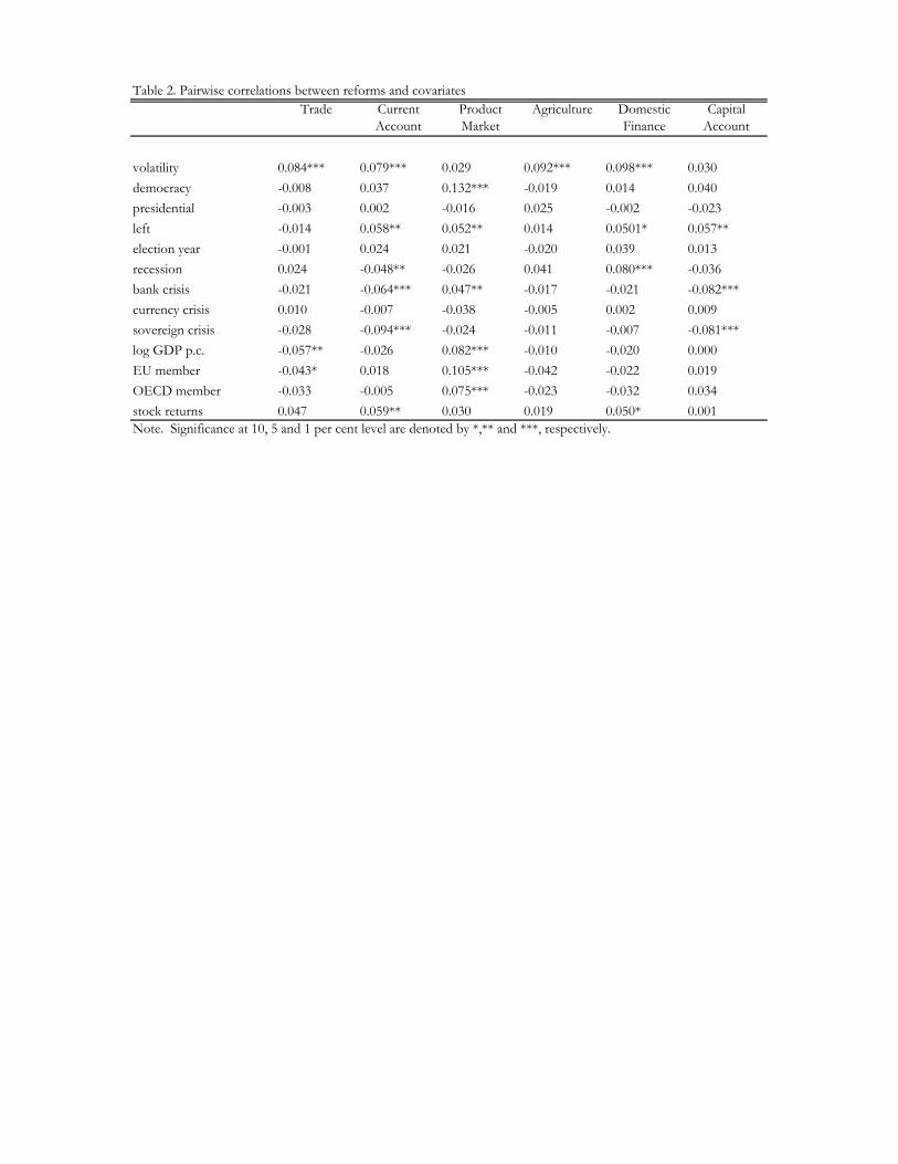
Trade Current Account

Product Market

Agriculture Domestic Finance

Capital Account

volatility 0.084*** 0.079*** 0.029 0.092*** 0.098*** 0.030

democracy -0.008 0.037 0.132*** -0.019 0.014 0.040

presidential -0.003 0.002 -0.016 0.025 -0.002 -0.023

left -0.014 0.058** 0.052** 0.014 0.0501* 0.057**

election year -0.001 0.024 0.021 -0.020 0.039 0.013

recession 0.024 -0.048** -0.026 0.041 0.080*** -0.036

bank crisis -0.021 -0.064*** 0.047** -0.017 -0.021 -0.082***

currency crisis 0.010 -0.007 -0.038 -0.005 0.002 0.009

sovereign crisis -0.028 -0.094*** -0.024 -0.011 -0.007 -0.081***

log GDP p.c. -0.057** -0.026 0.082*** -0.010 -0.020 0.000

EU member -0.043* 0.018 0.105*** -0.042 -0.022 0.019

OECD member -0.033 -0.005 0.075*** -0.023 -0.032 0.034

stock returns 0.047 0.059** 0.030 0.019 0.050* 0.001

Table 2. Pairwise correlations between reforms and covariates

Note. Significance at 10, 5 and 1 per cent level are denoted by *,** and ***, respectively.

(1) (2) (3) (4) (5) (6) (7)

liberalization -0.086*** -0.109*** -0.092*** -0.114*** -0.125*** -0.151***[0.005] [0.006] [0.005] [0.006] [0.007] [0.007]

volatility 0.705*** 0.504*** 0.431*** 0.695*** 0.395*** 0.472*** 0.442***[0.138] [0.138] [0.150] [0.143] [0.146] [0.155] [0.164]

democracy 0.026*** 0.017** 0.005[0.007] [0.007] [0.007]

presidential 0.015** 0.016** 0.015**[0.006] [0.006] [0.006]

left 0.008*** 0.007*** 0.004[0.002] [0.003] [0.003]

election year -0.000 0.001 0.001[0.002] [0.002] [0.002]

recession -0.005** -0.002 -0.003[0.002] [0.003] [0.003]

bank crisis -0.011** -0.010* -0.011**[0.005] [0.005] [0.005]

currency crisis -0.013** -0.012** -0.012**[0.005] [0.005] [0.005]

sovereign crisis -0.038*** -0.037*** -0.040***[0.010] [0.010] [0.010]

log GDP per capita 0.035*** 0.025*** -0.025***[0.005] [0.006] [0.009]

EU member 0.024*** 0.022*** 0.018***[0.006] [0.006] [0.006]

OECD member -0.011 -0.013 -0.004[0.009] [0.009] [0.009]

Country-Sector FE Yes Yes Yes Yes Yes Yes YesYear FE No No No No No No YesObservations 6.402 6.402 5.565 6.269 5.875 5.529 5.529R-squared 0.004 0.050 0.064 0.060 0.061 0.076 0.096Durbin-Watson 1.917 1.852 1.85 1.846 1.839 1.839 1.824

Table 3. OLS Regressions with AR(1) residualsDependent variable: annual change in liberalization indices

Notes. All regressors are expressed in one-year lags, except for EU membership, which is 2-year lead. AR(1) residuals are estimated with two-step procedure. The modified Bhargava et al. (1982) Durbin-Watson test for serially autocorrelated residuals is reported. Standard errors are reported in brackets. *, ** and *** denote significance at 10, 5 and 1 per cent, respectively.

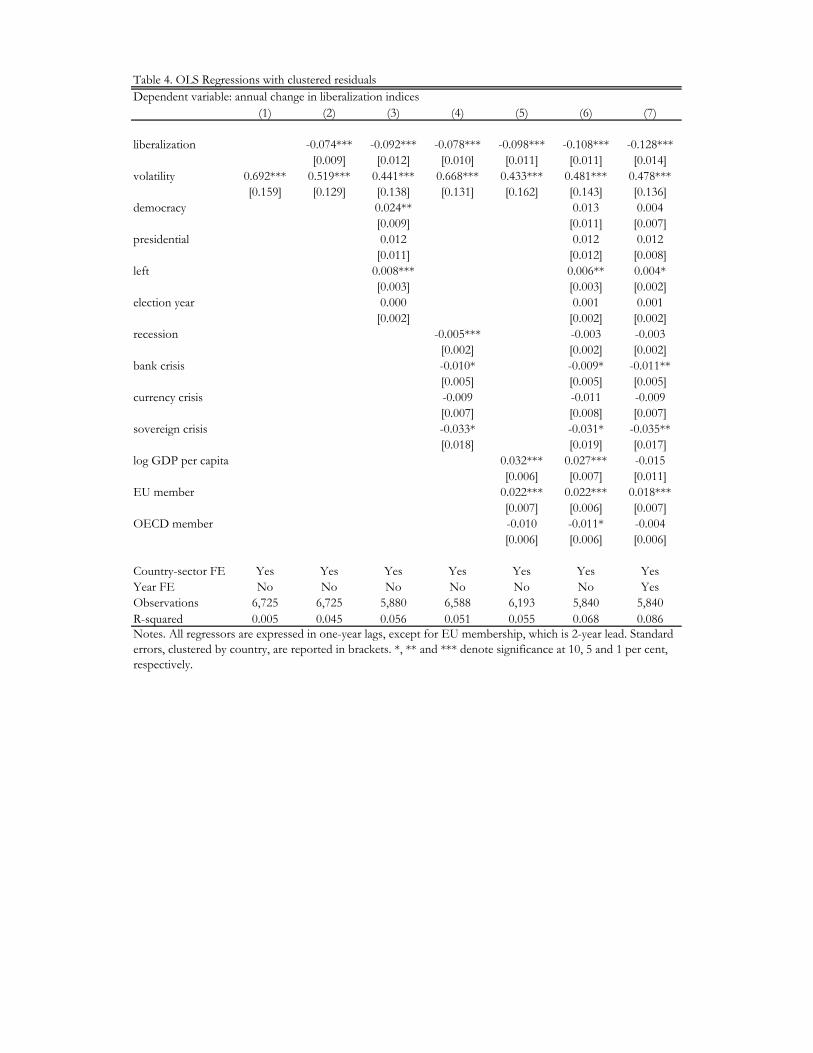
(1) (2) (3) (4) (5) (6) (7)

liberalization -0.074*** -0.092*** -0.078*** -0.098*** -0.108*** -0.128***[0.009] [0.012] [0.010] [0.011] [0.011] [0.014]

volatility 0.692*** 0.519*** 0.441*** 0.668*** 0.433*** 0.481*** 0.478***[0.159] [0.129] [0.138] [0.131] [0.162] [0.143] [0.136]

democracy 0.024** 0.013 0.004[0.009] [0.011] [0.007]

presidential 0.012 0.012 0.012[0.011] [0.012] [0.008]

left 0.008*** 0.006** 0.004*[0.003] [0.003] [0.002]

election year 0.000 0.001 0.001[0.002] [0.002] [0.002]

recession -0.005*** -0.003 -0.003[0.002] [0.002] [0.002]

bank crisis -0.010* -0.009* -0.011**[0.005] [0.005] [0.005]

currency crisis -0.009 -0.011 -0.009[0.007] [0.008] [0.007]

sovereign crisis -0.033* -0.031* -0.035**[0.018] [0.019] [0.017]

log GDP per capita 0.032*** 0.027*** -0.015[0.006] [0.007] [0.011]

EU member 0.022*** 0.022*** 0.018***[0.007] [0.006] [0.007]

OECD member -0.010 -0.011* -0.004[0.006] [0.006] [0.006]

Country-sector FE Yes Yes Yes Yes Yes Yes YesYear FE No No No No No No YesObservations 6,725 6,725 5,880 6,588 6,193 5,840 5,840R-squared 0.005 0.045 0.056 0.051 0.055 0.068 0.086

Table 4. OLS Regressions with clustered residualsDependent variable: annual change in liberalization indices

Notes. All regressors are expressed in one-year lags, except for EU membership, which is 2-year lead. Standard errors, clustered by country, are reported in brackets. *, ** and *** denote significance at 10, 5 and 1 per cent, respectively.

AR AR Clustered SE

Clustered SE

(1) (2) (3) (4)

liberalization -0.118*** -0.151*** -0.097*** -0.128***[0.006] [0.007] [0.010] [0.014]

volatility 0.613* 0.953** 0.492* 0.869***[0.351] [0.373] [0.279] [0.228]

volatility*Curr 0.051 -0.318 0.367 -0.039[0.479] [0.512] [0.930] [0.774]

volatility*PM -0.741 -0.909* -0.633 -0.960[0.480] [0.512] [0.606] [0.711]

volatility*AG 0.191 -0.037 0.360 0.067[0.484] [0.517] [0.742] [0.918]

volatility*DF -0.242 -0.510 0.135 -0.288[0.485] [0.512] [0.362] [0.378]

volatility*Cap -0.736 -1.262** -0.559 -1.095***[0.479] [0.512] [0.437] [0.358]

All Controls No Yes No YesCountry-Sector FE Yes Yes Yes YesYear FE Yes Yes Yes YesObservations 6.402 5.529 6.725 5.840R-squared 0.073 0.098 0.065 0.088

Table 5. OLS Regressions - Heterogeneous coefficients for volatilityDependent variable: annual change in liberalization indices

Notes. All regressors are expressed in one-year lags, except for EUmembership, which is 2-year lead. Volatility is interated with sectordummies for current account, product market, agriculture, domesticfinance and capital account. AR denotes AR(1) residuals, estimated withtwo-step procedure. Clustering denotes standard errors clustered bycountry. Standard errors are reported in brackets. *, ** and *** denotesignificance at 10, 5 and 1 per cent, respectively.

AR Clustered SE Probit Clustered SE

Logit AR Clustered SE Probit Clustered SE

Logit

(1) (2) (3) (4) (5) (6) (7) (8)

liberalization -0.128*** -0.107*** -0.503*** -4.860*** -0.101*** -0.090*** -0.379*** -8.027***[0.006] [0.011] [0.059] [0.408] [0.006] [0.010] [0.087] [0.728]

volatility 0.317** 0.344** 1.539* 14.493** 0.244* 0.271*** 0.865 19.910*[0.145] [0.130] [0.786] [7.116] [0.133] [0.098] [0.779] [11.353]

All Controls Yes Yes Yes Yes Yes Yes Yes YesCountry-Sector FE Yes Yes Yes Yes Yes Yes Yes YesYear FE Yes Yes Yes Yes Yes Yes Yes YesObservations 5,529 5,840 4,369 4,369 5,529 5,840 2,934 2,934R-squared 0.092 0.077 0.072 0.062

Table 6. Major reforms: OLS, Probit and Logit Regressions

Note. The dependent variable is equal to the annual change in the liberalization index if this is larger than the median (80thpercentile) positive annual change, in columns 1 and 2 (5 and 6); and it is a dummy taking value 1 if the annual change in theliberalization index is larger than the median (80th percentile) positive annual change, in columns 3 and 4 (7 and 8). Allregressors are expressed in one-year lags, except for EU membership, which is 2-year lead, and volatility where speficied. ARdenotes AR(1) residuals, estimated with two-step procedure. Clustering denotes standard errors clustered by country. Thestandard errors from Probit estimates are clustered by country. Standard errors are reported in brackets. *, ** and *** denotesignificance at 10, 5 and 1 per cent, respectively.

Dependent variable: positive annual changes in liberalization indices (reforms) - values and dummiesReforms above median Reforms above 80th percentile

AR Clustered SE AR Clustered SE AR Clustered SE(1) (2) (3) (4) (5) (6)

liberalization -0.146*** -0.124*** -0.143*** -0.119*** -0.152*** -0.154***[0.007] [0.015] [0.007] [0.014] [0.008] [0.016]

volatility 0.257 0.309*** 0.408** 0.414*** 0.289* 0.286**[0.162] [0.109] [0.162] [0.146] [0.173] [0.134]

All Controls Yes Yes Yes Yes Yes YesCountry-Sector FE Yes Yes Yes Yes Yes YesYear FE Yes Yes Yes Yes Yes YesObservations 5,316 5,627 5,102 5,413 5,529 5,840R-squared 0.091 0.083 0.092 0.080 0.089 0.089

Table 7. OLS Regressions: lagged volatility and cumulated reforms

Note. The dependent variable is the annual change in liberalization indices (columns 1-4), or the changein liberalization indices over the 3-year period starting with a non-zero annual change (columns 5-6). Allregressors are expressed in one-year lags, except for EU membership, which is 2-year lead, andvolatility where speficied. AR denotes AR(1) residuals, estimated with two-step procedure. Clusteringdenotes standard errors clustered by country. Standard errors are reported in brackets. *, ** and ***denote significance at 10, 5 and 1 per cent, respectively.

Dependent variable: annual/3-year (forward) change in liberalization indicesvolatility(t-2) volatility(t-3) 3-year cumulated reforms

IV first stage

IV second stage

IV first stage

IV second stage

AR AR Clustered SE

Clustered SE

(1) (2) (3) (4) (5) (6) (7) (8)

volatility 3.425*** 2.756***[0.487] [0.668]

volatility rest 0.609*** 0.627*** 3.476*** 3.422*** 2.871*** 3.239***[0.027] [0.038] [0.264] [0.361] [0.310] [0.525]

liberalization -0.008*** -0.065*** -0.008*** -0.097*** -0.079*** -0.102*** -0.070*** -0.090***[0.000] [0.005] [0.001] [0.007] [0.004] [0.005] [0.007] [0.009]

democracy -0.002*** 0.014** 0.021*** 0.020**[0.001] [0.007] [0.005] [0.009]

presidential 0.006*** -0.002 0.003 0.002[0.001] [0.007] [0.005] [0.006]

left 0.000 0.005** 0.003 0.002[0.000] [0.002] [0.002] [0.002]

election year 0.000 0.000 0.001 0.001[0.000] [0.002] [0.002] [0.001]

recession 0.002*** -0.008*** 0.002 0.002[0.000] [0.003] [0.002] [0.003]

bank crisis 0.004*** -0.017*** -0.014*** -0.013***[0.000] [0.006] [0.004] [0.004]

currency crisis 0.002*** -0.017*** -0.008* -0.007[0.000] [0.006] [0.004] [0.004]

sovereign crisis 0.003*** -0.040*** -0.030*** -0.031***[0.001] [0.011] [0.007] [0.010]

log GDP per capita -0.001 0.017*** -0.004 -0.003[0.001] [0.006] [0.005] [0.008]

EU member 0.002*** 0.017*** 0.018*** 0.017***[0.001] [0.006] [0.005] [0.003]

OECD member -0.001 -0.008 0.006 0.003[0.001] [0.008] [0.007] [0.006]

Country-Sector FE Yes Yes Yes Yes Yes Yes Yes YesObservations 6,721 6,721 5,840 5,840 9,673 8,090 9,998 8,408R-squared 0.0395 0.0550 0.034 0.050F-test 501.1 269.9

Table 8. 2SLS IV and OLS Regressions with volatility of the other countriesDependent variable: annual change in liberalization indices (except for IV first stage)

Notes. In columns (1) and (3), the dependent variable is stock market volatility, while in the other columns it is the annualchange in the liberalization indices. All regressors are expressed in one-year lags, except for EU membership, which is 2-yearlead. IV specifications are estimated with 2SLS. AR denotes AR(1) residuals, estimated with a two-stage procedure. ClusteredSE denotes standard errors clustered by country. The F-test for weak instruments is reported in the last row. Standard errorsare reported in brackets. *, ** and *** denote significance at 10, 5 and 1 per cent, respectively.

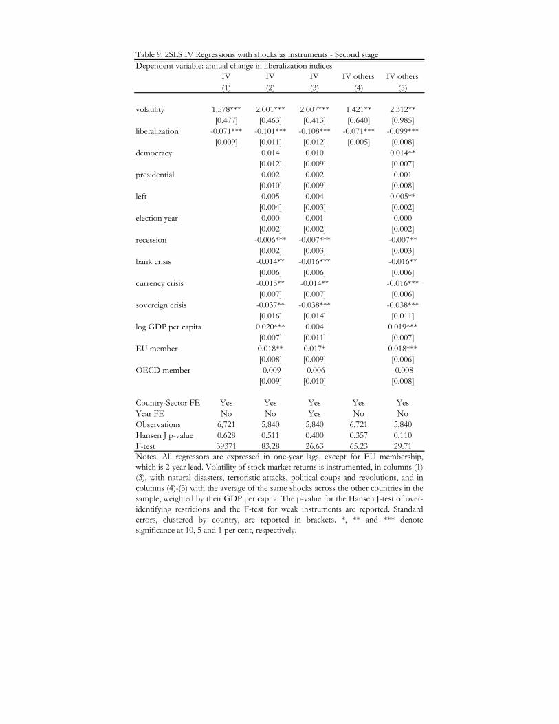
IV IV IV IV others IV others(1) (2) (3) (4) (5)

volatility 1.578*** 2.001*** 2.007*** 1.421** 2.312**[0.477] [0.463] [0.413] [0.640] [0.985]

liberalization -0.071*** -0.101*** -0.108*** -0.071*** -0.099***[0.009] [0.011] [0.012] [0.005] [0.008]

democracy 0.014 0.010 0.014**[0.012] [0.009] [0.007]

presidential 0.002 0.002 0.001[0.010] [0.009] [0.008]

left 0.005 0.004 0.005**[0.004] [0.003] [0.002]

election year 0.000 0.001 0.000[0.002] [0.002] [0.002]

recession -0.006*** -0.007*** -0.007**[0.002] [0.003] [0.003]

bank crisis -0.014** -0.016*** -0.016**[0.006] [0.006] [0.006]

currency crisis -0.015** -0.014** -0.016***[0.007] [0.007] [0.006]

sovereign crisis -0.037** -0.038*** -0.038***[0.016] [0.014] [0.011]

log GDP per capita 0.020*** 0.004 0.019***[0.007] [0.011] [0.007]

EU member 0.018** 0.017* 0.018***[0.008] [0.009] [0.006]

OECD member -0.009 -0.006 -0.008[0.009] [0.010] [0.008]

Country-Sector FE Yes Yes Yes Yes YesYear FE No No Yes No NoObservations 6,721 5,840 5,840 6,721 5,840Hansen J p-value 0.628 0.511 0.400 0.357 0.110F-test 39371 83.28 26.63 65.23 29.71Notes. All regressors are expressed in one-year lags, except for EU membership,which is 2-year lead. Volatility of stock market returns is instrumented, in columns (1)-(3), with natural disasters, terroristic attacks, political coups and revolutions, and incolumns (4)-(5) with the average of the same shocks across the other countries in thesample, weighted by their GDP per capita. The p-value for the Hansen J-test of over-identifying restricions and the F-test for weak instruments are reported. Standarderrors, clustered by country, are reported in brackets. *, ** and *** denotesignificance at 10, 5 and 1 per cent, respectively.

Table 9. 2SLS IV Regressions with shocks as instruments - Second stageDependent variable: annual change in liberalization indices

IV IV IV IV others IV others(1) (2) (3) (4) (5)

natural disasters -0.002 -0.001 -0.002 0.034*** 0.017***[0.002] [0.001] [0.001] [0.005] [0.005]

coups 0.022** 0.021** 0.020** -0.048** -0.034[0.010] [0.009] [0.009] [0.021] [0.022]

revolutions 0.057*** 0.047*** 0.039*** 2.878*** 2.097***[0.000] [0.003] [0.004] [0.197] [0.203]

terrorist attaks 0.001 0.000 0.001 0.026*** 0.001[0.001] [0.001] [0.001] [0.006] [0.006]

Country-Sector FE Yes Yes Yes Yes YesYear FE No No Yes No NoObservations 6,721 5,840 5,840 6,721 5,840

Table 10. 2SLS IV Regressions with shocks as instruments - First stageDependent variable: stock market volatility

Notes. All regressors are expressed in one-year lags. The instruments refer to eachcountry in columns (1)-(3), to the average of the other countries in the sample,weighted by their GDP p.c. in columns (4)-(5). Coefficients for lagged liberalizationand the other controls are omitted. Standard errors, clustered by country, arereported in brackets. *, ** and *** denote significance at 10, 5 and 1 per cent,respectively.

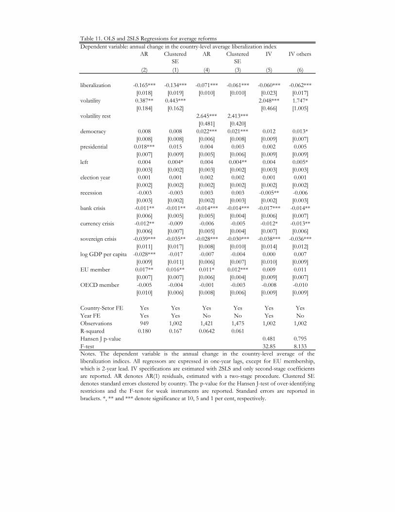
AR Clustered SE

AR Clustered SE

IV IV others

(2) (1) (4) (3) (5) (6)

liberalization -0.165*** -0.134*** -0.071*** -0.061*** -0.060*** -0.062***[0.018] [0.019] [0.010] [0.010] [0.023] [0.017]

volatility 0.387** 0.443*** 2.048*** 1.747*[0.184] [0.162] [0.466] [1.005]

volatility rest 2.645*** 2.413***[0.481] [0.420]

democracy 0.008 0.008 0.022*** 0.021*** 0.012 0.013*[0.008] [0.008] [0.006] [0.008] [0.009] [0.007]

presidential 0.018*** 0.015 0.004 0.003 0.002 0.005[0.007] [0.009] [0.005] [0.006] [0.009] [0.009]

left 0.004 0.004* 0.004 0.004** 0.004 0.005*[0.003] [0.002] [0.003] [0.002] [0.003] [0.003]

election year 0.001 0.001 0.002 0.002 0.001 0.001[0.002] [0.002] [0.002] [0.002] [0.002] [0.002]

recession -0.003 -0.003 0.003 0.003 -0.005** -0.006[0.003] [0.002] [0.002] [0.003] [0.002] [0.003]

bank crisis -0.011** -0.011** -0.014*** -0.014*** -0.017*** -0.014**[0.006] [0.005] [0.005] [0.004] [0.006] [0.007]

currency crisis -0.012** -0.009 -0.006 -0.005 -0.012* -0.013**[0.006] [0.007] [0.005] [0.004] [0.007] [0.006]

sovereign crisis -0.039*** -0.035** -0.028*** -0.030*** -0.038*** -0.036***[0.011] [0.017] [0.008] [0.010] [0.014] [0.012]

log GDP per capita -0.028*** -0.017 -0.007 -0.004 0.000 0.007[0.009] [0.011] [0.006] [0.007] [0.010] [0.009]

EU member 0.017** 0.016** 0.011* 0.012*** 0.009 0.011[0.007] [0.007] [0.006] [0.004] [0.009] [0.007]

OECD member -0.005 -0.004 -0.001 -0.003 -0.008 -0.010[0.010] [0.006] [0.008] [0.006] [0.009] [0.009]

Country-Setor FE Yes Yes Yes Yes Yes YesYear FE Yes Yes No No Yes NoObservations 949 1,002 1,421 1,475 1,002 1,002R-squared 0.180 0.167 0.0642 0.061Hansen J p-value 0.481 0.795F-test 32.85 8.133

Table 11. OLS and 2SLS Regressions for average reformsDependent variable: annual change in the country-level average liberalization index

Notes. The dependent variable is the annual change in the country-level average of theliberalization indices. All regressors are expressed in one-year lags, except for EU membership,which is 2-year lead. IV specifications are estimated with 2SLS and only second-stage coefficientsare reported. AR denotes AR(1) residuals, estimated with a two-stage procedure. Clustered SEdenotes standard errors clustered by country. The p-value for the Hansen J-test of over-identifyingrestricions and the F-test for weak instruments are reported. Standard errors are reported inbrackets. *, ** and *** denote significance at 10, 5 and 1 per cent, respectively.

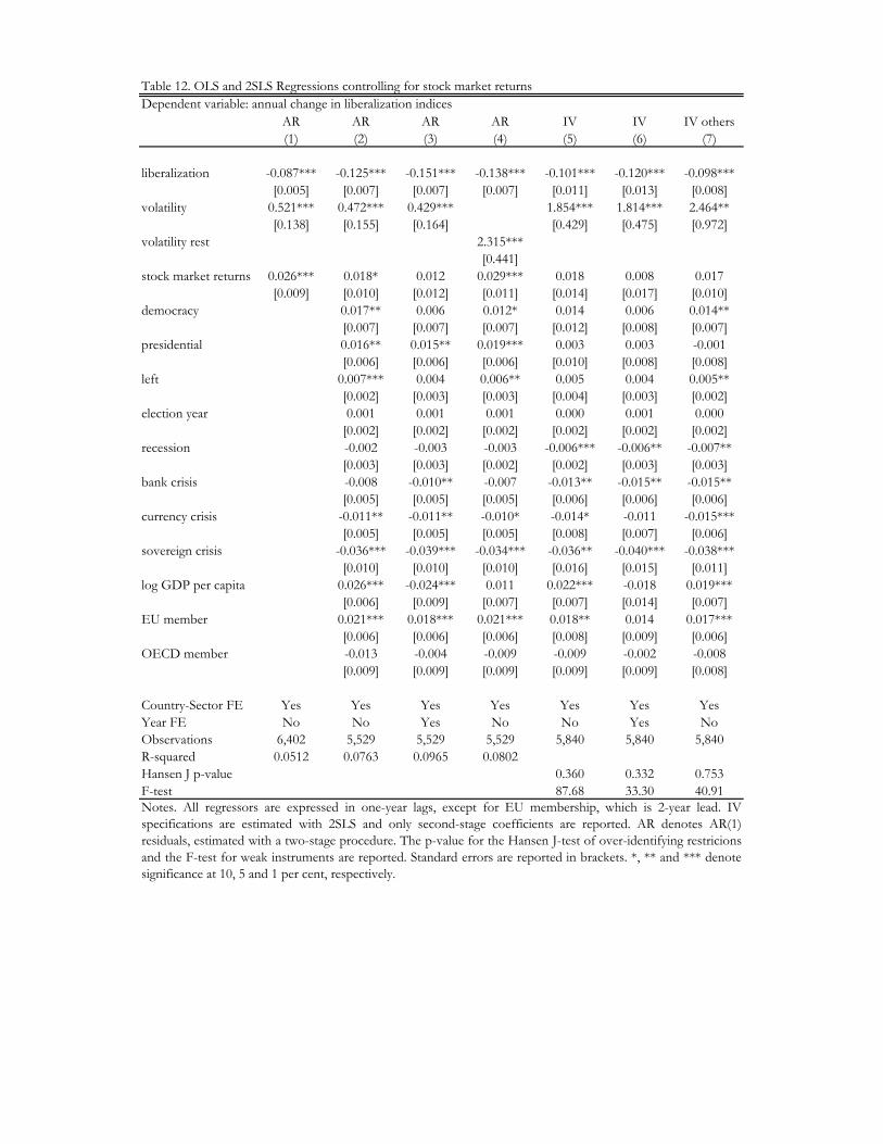
AR AR AR AR IV IV IV others(1) (2) (3) (4) (5) (6) (7)

liberalization -0.087*** -0.125*** -0.151*** -0.138*** -0.101*** -0.120*** -0.098***[0.005] [0.007] [0.007] [0.007] [0.011] [0.013] [0.008]

volatility 0.521*** 0.472*** 0.429*** 1.854*** 1.814*** 2.464**[0.138] [0.155] [0.164] [0.429] [0.475] [0.972]

volatility rest 2.315***[0.441]

stock market returns 0.026*** 0.018* 0.012 0.029*** 0.018 0.008 0.017[0.009] [0.010] [0.012] [0.011] [0.014] [0.017] [0.010]

democracy 0.017** 0.006 0.012* 0.014 0.006 0.014**[0.007] [0.007] [0.007] [0.012] [0.008] [0.007]

presidential 0.016** 0.015** 0.019*** 0.003 0.003 -0.001[0.006] [0.006] [0.006] [0.010] [0.008] [0.008]

left 0.007*** 0.004 0.006** 0.005 0.004 0.005**[0.002] [0.003] [0.003] [0.004] [0.003] [0.002]

election year 0.001 0.001 0.001 0.000 0.001 0.000[0.002] [0.002] [0.002] [0.002] [0.002] [0.002]

recession -0.002 -0.003 -0.003 -0.006*** -0.006** -0.007**[0.003] [0.003] [0.002] [0.002] [0.003] [0.003]

bank crisis -0.008 -0.010** -0.007 -0.013** -0.015** -0.015**[0.005] [0.005] [0.005] [0.006] [0.006] [0.006]

currency crisis -0.011** -0.011** -0.010* -0.014* -0.011 -0.015***[0.005] [0.005] [0.005] [0.008] [0.007] [0.006]

sovereign crisis -0.036*** -0.039*** -0.034*** -0.036** -0.040*** -0.038***[0.010] [0.010] [0.010] [0.016] [0.015] [0.011]

log GDP per capita 0.026*** -0.024*** 0.011 0.022*** -0.018 0.019***[0.006] [0.009] [0.007] [0.007] [0.014] [0.007]

EU member 0.021*** 0.018*** 0.021*** 0.018** 0.014 0.017***[0.006] [0.006] [0.006] [0.008] [0.009] [0.006]

OECD member -0.013 -0.004 -0.009 -0.009 -0.002 -0.008[0.009] [0.009] [0.009] [0.009] [0.009] [0.008]

Country-Sector FE Yes Yes Yes Yes Yes Yes YesYear FE No No Yes No No Yes NoObservations 6,402 5,529 5,529 5,529 5,840 5,840 5,840R-squared 0.0512 0.0763 0.0965 0.0802Hansen J p-value 0.360 0.332 0.753F-test 87.68 33.30 40.91

Dependent variable: annual change in liberalization indicesTable 12. OLS and 2SLS Regressions controlling for stock market returns

Notes. All regressors are expressed in one-year lags, except for EU membership, which is 2-year lead. IVspecifications are estimated with 2SLS and only second-stage coefficients are reported. AR denotes AR(1)residuals, estimated with a two-stage procedure. The p-value for the Hansen J-test of over-identifying restricionsand the F-test for weak instruments are reported. Standard errors are reported in brackets. *, ** and *** denotesignificance at 10, 5 and 1 per cent, respectively.

AR AR AR AR AR AR AR AR(1) (2) (3) (4) (5) (6) (7) (8)

liberalization -0.154*** -0.151*** -0.152*** -0.149*** -0.128*** -0.138*** -0.128*** -0.138***[0.007] [0.007] [0.007] [0.007] [0.007] [0.007] [0.007] [0.007]

volatility 0.429*** 0.441***[0.164] [0.163]

volatility rest 2.315*** 2.322***[0.441] [0.441]

stock market returns 0.014 0.012 0.014 0.012 0.018* 0.029*** 0.018* 0.029***[0.012] [0.012] [0.012] [0.012] [0.010] [0.011] [0.010] [0.011]

democracy 0.005 0.006 0.005 0.006 0.016** 0.012* 0.016** 0.012*[0.007] [0.007] [0.007] [0.007] [0.007] [0.007] [0.007] [0.007]

presidential 0.018*** 0.015** 0.018*** 0.015** 0.019*** 0.019*** 0.018*** 0.018***[0.006] [0.006] [0.006] [0.006] [0.006] [0.006] [0.006] [0.006]

left 0.004 0.004 0.004 0.004 0.007*** 0.006** 0.007*** 0.006**[0.003] [0.003] [0.003] [0.003] [0.003] [0.003] [0.003] [0.003]

election year 0.001 0.001 0.001 0.000 0.001 0.001 0.001 0.001[0.002] [0.002] [0.002] [0.002] [0.002] [0.002] [0.002] [0.002]

recession -0.002 -0.003 -0.002 -0.003[0.003] [0.003] [0.002] [0.002]

growth GDP p.c. 0.036 0.047 0.027 0.040[0.032] [0.033] [0.031] [0.031]

bank crisis -0.009* -0.010** -0.008 -0.010* -0.007 -0.007 -0.006 -0.006[0.005] [0.005] [0.005] [0.005] [0.005] [0.005] [0.005] [0.005]

currency crisis -0.010* -0.011** -0.009* -0.010* -0.010* -0.010* -0.009 -0.010*[0.005] [0.005] [0.006] [0.006] [0.005] [0.005] [0.005] [0.005]

sovereign crisis -0.037*** -0.039*** -0.038*** -0.040*** -0.034*** -0.034*** -0.034*** -0.034***[0.010] [0.010] [0.010] [0.010] [0.010] [0.010] [0.010] [0.010]

log GDP per capita -0.023*** -0.024*** -0.023*** -0.024*** 0.028*** 0.011 0.028*** 0.011[0.009] [0.009] [0.009] [0.009] [0.006] [0.007] [0.006] [0.007]

EU member 0.019*** 0.018*** 0.019*** 0.018*** 0.022*** 0.021*** 0.022*** 0.021***[0.006] [0.006] [0.006] [0.006] [0.006] [0.006] [0.006] [0.006]

OECD member -0.003 -0.004 -0.003 -0.004 -0.013 -0.009 -0.012 -0.008[0.009] [0.009] [0.009] [0.009] [0.009] [0.009] [0.009] [0.009]

Country-Sector FE Yes Yes Yes Yes Yes Yes Yes YesYear FE Yes Yes Yes Yes No No No NoObservations 5,529 5,529 5,529 5,529 5,529 5,529 5,529 5,529R-squared 0.0956 0.0965 0.0947 0.0956 0.0749 0.0802 0.0749 0.0802

Dependent variable: annual change in liberalization indicesTable 13. OLS Regressions - volatility vs crises and GDP growth

Notes. All regressors are expressed in one-year lags, except for EU membership, which is 2-year lead. AR denotes AR(1)residuals, estimated with a two-stage procedure. Standard errors are reported in brackets. *, ** and *** denote significance at10, 5 and 1 per cent, respectively.

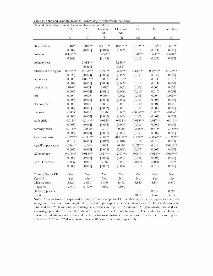
AR AR Clustered SE

Clustered SE

IV IV IV others

(1) (2) (3) (4) (5) (6) (7)

liberalization -0.148*** -0.101*** -0.118*** -0.090*** -0.102*** -0.105*** -0.101***[0.007] [0.005] [0.013] [0.009] [0.011] [0.011] [0.008]

volatility 0.448*** 0.464*** 1.941*** 1.841*** 2.088**[0.162] [0.133] [0.415] [0.427] [0.985]

volatility rest 3.314*** 3.139***[0.360] [0.521]

reforms in the region 0.092*** 0.108*** 0.097** 0.120*** 0.129*** 0.096*** 0.128***[0.028] [0.024] [0.036] [0.029] [0.037] [0.035] [0.027]

democracy 0.005 0.021*** 0.007 0.019** 0.013 0.011 0.013*[0.007] [0.005] [0.008] [0.009] [0.012] [0.011] [0.007]

presidential 0.016** 0.004 0.012 0.002 0.003 0.003 0.003[0.006] [0.004] [0.011] [0.006] [0.010] [0.010] [0.008]

left 0.004 0.003 0.004* 0.002 0.005 0.004 0.005**[0.003] [0.002] [0.002] [0.002] [0.004] [0.003] [0.002]

election year 0.000 0.001 0.001 0.001 0.000 0.001 0.000[0.002] [0.002] [0.002] [0.001] [0.002] [0.002] [0.002]

recession -0.003 0.002 -0.004 0.002 -0.006*** -0.005** -0.006*[0.003] [0.002] [0.002] [0.003] [0.002] [0.002] [0.003]

bank crisis -0.011** -0.014*** -0.012** -0.014*** -0.015*** -0.017*** -0.016**[0.005] [0.004] [0.005] [0.004] [0.006] [0.006] [0.006]

currency crisis -0.011** -0.008* -0.010 -0.007 -0.015** -0.013* -0.015***[0.005] [0.004] [0.007] [0.004] [0.007] [0.007] [0.006]

sovereign crisis -0.039*** -0.030*** -0.032* -0.031*** -0.036** -0.036*** -0.036***[0.010] [0.007] [0.017] [0.010] [0.016] [0.013] [0.011]

log GDP per capita -0.024*** -0.004 0.009 -0.003 0.021*** 0.014 0.021***[0.009] [0.005] [0.008] [0.008] [0.007] [0.009] [0.007]

EU member 0.018*** 0.018*** 0.021*** 0.017*** 0.019** 0.018** 0.019***[0.006] [0.005] [0.006] [0.003] [0.008] [0.008] [0.006]

OECD member -0.006 0.006 -0.007 0.003 -0.009 -0.008 -0.009[0.009] [0.007] [0.007] [0.006] [0.010] [0.010] [0.008]

Country-Sector FE Yes Yes Yes Yes Yes Yes YesYear FE Yes No Yes No No Yes NoObservations 5,529 8,090 5,840 8,408 5,840 5,840 5,840R-squared 0.0970 0.0569 0.083 0.053Hansen J p-value 0.319 0.347 0.765F-test 108.8 33.67 39.19

Dependent variable: annual change in liberalization indicesTable 14. OLS and 2SLS Regressions - controlling for reforms in the region

Notes. All regressors are expressed in one-year lags, except for EU membership, which is 2-year lead, and theaverage reform in the region, weighted by real GDP per capita, which is contemporaneous. IV specifications areestimated with 2SLS and only second-stage coefficients are reported. AR denotes AR(1) residuals, estimated witha two-stage procedure. Clustered SE denotes standard errors clustered by country. The p-value for the Hansen J-test of over-identifying restricions and the F-test for weak instruments are reported. Standard errors are reportedin brackets. *, ** and *** denote significance at 10, 5 and 1 per cent, respectively.

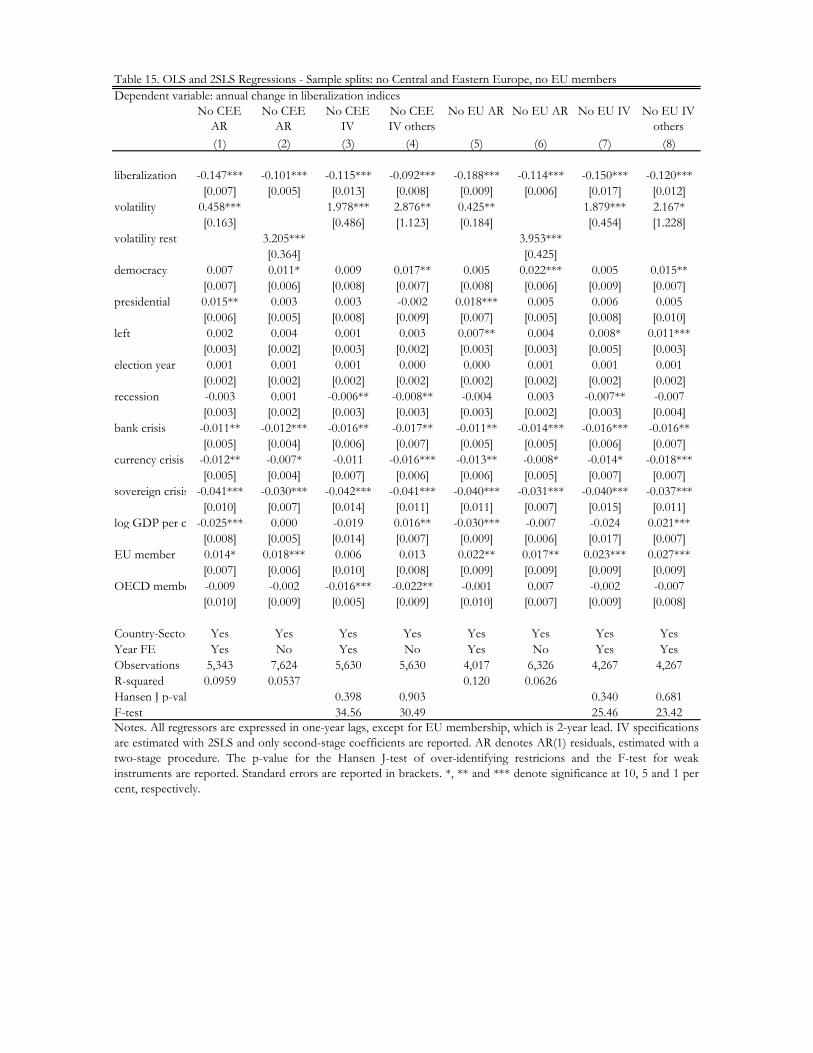
No CEE AR

No CEE AR

No CEE IV

No CEE IV others

No EU AR No EU AR No EU IV No EU IV others

(1) (2) (3) (4) (5) (6) (7) (8)

liberalization -0.147*** -0.101*** -0.115*** -0.092*** -0.188*** -0.114*** -0.150*** -0.120***[0.007] [0.005] [0.013] [0.008] [0.009] [0.006] [0.017] [0.012]

volatility 0.458*** 1.978*** 2.876** 0.425** 1.879*** 2.167*[0.163] [0.486] [1.123] [0.184] [0.454] [1.228]

volatility rest 3.205*** 3.953***[0.364] [0.425]

democracy 0.007 0.011* 0.009 0.017** 0.005 0.022*** 0.005 0.015**[0.007] [0.006] [0.008] [0.007] [0.008] [0.006] [0.009] [0.007]

presidential 0.015** 0.003 0.003 -0.002 0.018*** 0.005 0.006 0.005[0.006] [0.005] [0.008] [0.009] [0.007] [0.005] [0.008] [0.010]

left 0.002 0.004 0.001 0.003 0.007** 0.004 0.008* 0.011***[0.003] [0.002] [0.003] [0.002] [0.003] [0.003] [0.005] [0.003]

election year 0.001 0.001 0.001 0.000 0.000 0.001 0.001 0.001[0.002] [0.002] [0.002] [0.002] [0.002] [0.002] [0.002] [0.002]

recession -0.003 0.001 -0.006** -0.008** -0.004 0.003 -0.007** -0.007[0.003] [0.002] [0.003] [0.003] [0.003] [0.002] [0.003] [0.004]

bank crisis -0.011** -0.012*** -0.016** -0.017** -0.011** -0.014*** -0.016*** -0.016**[0.005] [0.004] [0.006] [0.007] [0.005] [0.005] [0.006] [0.007]

currency crisis -0.012** -0.007* -0.011 -0.016*** -0.013** -0.008* -0.014* -0.018***[0.005] [0.004] [0.007] [0.006] [0.006] [0.005] [0.007] [0.007]

sovereign crisis -0.041*** -0.030*** -0.042*** -0.041*** -0.040*** -0.031*** -0.040*** -0.037***[0.010] [0.007] [0.014] [0.011] [0.011] [0.007] [0.015] [0.011]

log GDP per c -0.025*** 0.000 -0.019 0.016** -0.030*** -0.007 -0.024 0.021***[0.008] [0.005] [0.014] [0.007] [0.009] [0.006] [0.017] [0.007]

EU member 0.014* 0.018*** 0.006 0.013 0.022** 0.017** 0.023*** 0.027***[0.007] [0.006] [0.010] [0.008] [0.009] [0.009] [0.009] [0.009]

OECD membe -0.009 -0.002 -0.016*** -0.022** -0.001 0.007 -0.002 -0.007[0.010] [0.009] [0.005] [0.009] [0.010] [0.007] [0.009] [0.008]

Country-Sector Yes Yes Yes Yes Yes Yes Yes YesYear FE Yes No Yes No Yes No Yes YesObservations 5,343 7,624 5,630 5,630 4,017 6,326 4,267 4,267R-squared 0.0959 0.0537 0.120 0.0626Hansen J p-valu 0.398 0.903 0.340 0.681F-test 34.56 30.49 25.46 23.42

Dependent variable: annual change in liberalization indicesTable 15. OLS and 2SLS Regressions - Sample splits: no Central and Eastern Europe, no EU members

Notes. All regressors are expressed in one-year lags, except for EU membership, which is 2-year lead. IV specificationsare estimated with 2SLS and only second-stage coefficients are reported. AR denotes AR(1) residuals, estimated with atwo-stage procedure. The p-value for the Hansen J-test of over-identifying restricions and the F-test for weakinstruments are reported. Standard errors are reported in brackets. *, ** and *** denote significance at 10, 5 and 1 percent, respectively.

low news high news low news high news low news high news(1) (2) (3) (4) (7) (8)

liberalization -0.196*** -0.104*** -0.111*** -0.088*** -0.120*** -0.080***[0.011] [0.009] [0.007] [0.008] [0.016] [0.008]

volatility 0.402** 0.471 2.273* 1.719[0.201] [0.428] [1.363] [1.319]

volatility rest 3.899*** 2.838***[0.484] [0.547]

democracy -0.001 -0.036 0.014** 0.059*** 0.017** -0.056**[0.009] [0.033] [0.006] [0.015] [0.009] [0.028]

presidential 0.016* 0.029** 0.004 -0.001 0.010 0.032**[0.009] [0.014] [0.006] [0.012] [0.015] [0.014]

left 0.002 0.005* 0.004 0.004 0.007 0.004[0.004] [0.003] [0.004] [0.003] [0.005] [0.003]

election year 0.001 -0.000 0.002 0.001 0.001 -0.000[0.003] [0.002] [0.002] [0.002] [0.003] [0.002]

recession -0.003 0.001 0.003 0.000 -0.007 -0.006[0.004] [0.004] [0.003] [0.003] [0.005] [0.004]

bank crisis -0.013** -0.003 -0.017*** -0.003 -0.020** -0.003[0.007] [0.009] [0.005] [0.008] [0.010] [0.008]

currency crisis -0.010 -0.026** -0.009* -0.012 -0.015* -0.021**[0.007] [0.011] [0.005] [0.008] [0.008] [0.010]

sovereign crisis -0.035*** -0.024*** -0.087*** -0.036***[0.012] [0.008] [0.019] [0.012]

log GDP per capita -0.035*** -0.009 0.001 -0.017* 0.032*** 0.016[0.013] [0.016] [0.006] [0.010] [0.009] [0.011]

EU member 0.033*** 0.012 0.021** 0.017*** 0.033*** 0.009[0.012] [0.007] [0.009] [0.006] [0.011] [0.006]

OECD member 0.005 -0.002 0.015* -0.010 0.010 -0.014[0.014] [0.013] [0.009] [0.011] [0.013] [0.011]

Country-Sector FE Yes Yes Yes Yes Yes YesYear FE Yes Yes No No No NoObservations 3,084 2,445 5,116 2,974 3,279 2,561R-squared 0.126 0.0778 0.0614 0.0523Hansen J p-value 0.263 0.350F-test 17.65 45.35

Table 16. OLS and 2SLS Regressions - low vs high newspapers circulation countriesDependent variable: annual change in liberalization indices

Notes. All regressors are expressed in one-year lags, except for EU membership, which is 2-yearlead. "low news" and "high news" denote countries with daily newspapers circulation below andabove the sample mean in 1996, respectively. IV specifications are estimated with 2SLS and onlysecond-stage coefficients are reported. AR denotes AR(1) residuals, estimated with a two-stageprocedure. The p-value for the Hansen J-test of over-identifying restricions and the F-test forweak instruments are reported. Standard errors are reported in brackets. *, ** and *** denotesignificance at 10, 5 and 1 per cent, respectively.

AR AR IV others

AR AR AR Clustered SE

Clustered SE

Clustered SE

IV IV others

(1) (2) (3) (4) (5) (6) (7) (8)

liberalization -0.095*** -0.105*** -0.066*** -0.083*** -0.086*** -0.056*** -0.080*** -0.082***[0.006] [0.007] [0.005] [0.009] [0.009] [0.007] [0.010] [0.007]

volatility 0.186 0.262* 0.186 0.266 1.432** 0.316[0.148] [0.156] [0.173] [0.178] [0.599] [0.924]

volatility rest 1.569*** 1.464***[0.347] [0.441]

democracy -0.016** -0.022*** 0.006 -0.019*** -0.022*** 0.005 -0.020*** -0.019***[0.007] [0.007] [0.005] [0.007] [0.008] [0.012] [0.006] [0.006]

presidential 0.012** 0.012** -0.004 0.010 0.010 -0.005 0.002 0.009[0.006] [0.006] [0.004] [0.009] [0.009] [0.005] [0.007] [0.008]

left 0.005** 0.003 0.000 0.004** 0.003 -0.001 0.003 0.004*[0.002] [0.002] [0.002] [0.002] [0.002] [0.002] [0.003] [0.002]

election year 0.002 0.001 0.002 0.001 0.001 0.002 0.001 0.001[0.002] [0.002] [0.002] [0.001] [0.001] [0.001] [0.001] [0.002]

recession 0.000 -0.000 0.004** 0.001 0.001 0.005* -0.002 0.001[0.002] [0.002] [0.002] [0.003] [0.002] [0.003] [0.002] [0.003]

bank crisis -0.002 -0.003 -0.002 -0.003 -0.005 0.000 -0.009 -0.004[0.005] [0.005] [0.004] [0.005] [0.005] [0.005] [0.006] [0.006]

currency crisis 0.002 0.002 -0.007* -0.003 -0.003 -0.006 -0.005 -0.003[0.005] [0.005] [0.004] [0.006] [0.006] [0.004] [0.007] [0.005]

sovereign crisis 0.003 0.003 -0.008 0.008 0.008 -0.009 0.004 0.007[0.010] [0.010] [0.006] [0.014] [0.017] [0.008] [0.019] [0.010]

log GDP per capita 0.029*** 0.005 0.007 0.027*** 0.018** 0.007 0.015** 0.027***[0.006] [0.008] [0.005] [0.006] [0.007] [0.006] [0.007] [0.006]

EU member 0.009 0.008 0.009* 0.009* 0.009* 0.008** 0.006 0.009[0.006] [0.006] [0.005] [0.005] [0.005] [0.004] [0.007] [0.006]

OECD member -0.006 -0.002 0.007 -0.007** -0.004 0.005 -0.003 -0.006[0.009] [0.009] [0.006] [0.003] [0.003] [0.009] [0.004] [0.007]

Country-Sector FE Yes Yes Yes Yes Yes Yes Yes YesYear FE No Yes No No Yes No Yes NoObservations 5,529 5,529 8,090 5,840 5,840 8,408 5,840 5,840R-squared 0.0468 0.0581 0.0235 0.045 0.054 0.020Hansen J p-value 0.363 0.238F-test 34.03 39.62

Dependent variable: absolute value of the annual change in liberalization indicesTable 17. OLS and 2SLS Regressions - absolute change in liberalization indices

Notes. The dependent variable is the absolute value of the annual change in the liberalization indices. All regressors areexpressed in one-year lags, except for EU membership, which is 2-year lead. IV specifications are estimated with 2SLS andonly second-stage coefficients are reported. AR denotes AR(1) residuals, estimated with a two-stage procedure. Clustered SEdenotes standard errors clustered by country. The p-value for the Hansen J-test of over-identifying restricions and the F-testfor weak instruments are reported. Standard errors are reported in brackets. *, ** and *** denote significance at 10, 5 and 1per cent, respectively.

AR AR Clustered SE

Clustered SE

IV IV others Abs. Change AR(1)

Abs. Change AR(1)

(1) (2) (3) (4) (5) (6) (7) (8)

abortion_index -0.265*** -0.226*** -0.214*** -0.176*** -0.215*** -0.219*** -0.263*** -0.117***[0.018] [0.014] [0.031] [0.038] [0.029] [0.016] [0.018] [0.014]

volatility -0.278 -0.310 0.484 0.352 -0.288[0.266] [0.376] [0.358] [1.715] [0.268]

volatility rest 0.597 0.159 -1.301*[0.659] [0.465] [0.666]

democracy -0.000 -0.010 0.004 -0.017 0.003 0.002 0.007 0.021**[0.013] [0.010] [0.019] [0.020] [0.017] [0.013] [0.013] [0.010]

presidential -0.011 -0.025*** -0.013 -0.022 -0.017 -0.014 -0.013 -0.010[0.009] [0.009] [0.013] [0.015] [0.013] [0.013] [0.010] [0.009]

left 0.002 -0.001 0.001 -0.002 0.001 0.001 0.000 -0.004[0.004] [0.004] [0.003] [0.005] [0.003] [0.004] [0.004] [0.004]

election year -0.002 0.003 -0.003 0.005 -0.003 -0.004 -0.001 -0.001[0.003] [0.003] [0.003] [0.004] [0.003] [0.003] [0.003] [0.003]

recession -0.003 0.002 -0.003 0.002 -0.004 -0.005 -0.003 0.003[0.004] [0.004] [0.004] [0.004] [0.004] [0.005] [0.004] [0.004]

bank crisis -0.000 -0.008 0.001 -0.006 -0.003 -0.001 -0.001 0.005[0.009] [0.008] [0.004] [0.006] [0.005] [0.012] [0.009] [0.009]

currency crisis 0.003 0.005 -0.000 0.006 -0.002 -0.001 0.003 0.003[0.009] [0.008] [0.004] [0.009] [0.003] [0.010] [0.009] [0.008]

sovereign crisis 0.015 -0.003 0.018** -0.005 0.016 0.013 0.013 -0.010[0.019] [0.013] [0.008] [0.006] [0.010] [0.019] [0.019] [0.013]

log GDP per capita 0.000 0.010 0.009 0.018 0.009 0.006 -0.005 0.013[0.014] [0.009] [0.012] [0.012] [0.011] [0.009] [0.015] [0.009]

EU member 0.014 0.017* 0.011 0.013 0.009 0.009 0.014 0.010[0.009] [0.010] [0.009] [0.014] [0.008] [0.009] [0.010] [0.010]

OECD member 0.002 -0.006 -0.001 -0.001 -0.000 0.000 0.001 -0.018[0.014] [0.013] [0.005] [0.007] [0.004] [0.013] [0.014] [0.013]

Country-Sector FE Yes Yes Yes Yes Yes Yes Yes YesYear FE Yes No Yes No Yes No Yes NoObservations 941 1,408 994 1,462 994 994 941 1,408R-squared 0.242 0.162 0.199 0.117 0.242 0.059Hansen J p-value 0.481 0.732F-test 100.6 6.229

Table 18. OLS and 2SLS Regressions - abortion reformsDependent variable: annual change in the abortion index

Notes. The dependent variable in columns 1-6 is the annual change in the average index capturing in how many, out of 7circumstances, abortion is legal. The dependent variable in columns 7-8 is the absolute value of the annual change in the averageabortion index All regressors are expressed in one-year lags, except for EU membership, which is 2-year lead. IV specificationsare estimated with 2SLS and only second-stage coefficients are reported. AR denotes AR(1) residuals, estimated with a two-stage procedure. Clustered SE denotes standard errors clustered by country. The p-value for the Hansen J-test of over-identifying restricions and the F-test for weak instruments are reported. Standard errors are reported in brackets. *, ** and ***denote significance at 10, 5 and 1 per cent, respectively.