Economic Liberalization and Wage Inequality in India

World Development Vol. 34, No. 12, pp. 1997–2015, 2006� 2006 Elsevier Ltd. All rights reserved

0305-750X/$ - see front matter

doi:10.1016/j.worlddev.2006.02.010www.elsevier.com/locate/worlddev

Economic Liberalization and Wage Inequality in India

RUBIANA CHAMARBAGWALA *

Indiana University, Bloomington, IN, USA

Summary. — We investigate India’s widening skill wage gap and narrowing gender wage differ-ential during the two decades that coincide with the economic liberalization in the country. Usingthe nonparametric methodology developed by Katz and Murphy [Katz, L. F., & Murphy, K. M.(1992). Changes in relative wages, 1963–87: supply and demand factors. Quarterly Journal of Eco-nomics, 107(1), 35–78], we find that relative demand shifts contributed to relative wage shifts andthat increases in the demand for skilled labor were mostly due to skill upgrading within industries.In assessing the contribution of external sector reforms to demand for skilled labor, we find thatinternational trade-in manufactures benefited skilled men but hurt skilled women, whereas out-sourcing of services generated a demand for both female and male college graduates.
� 2006 Elsevier Ltd. All rights reserved.
JEL classification — F16, J24, J31Key words — trade and labor market interactions, education, wages, Asia, India

* Final revision accepted: February 27, 2006.

1. INTRODUCTION

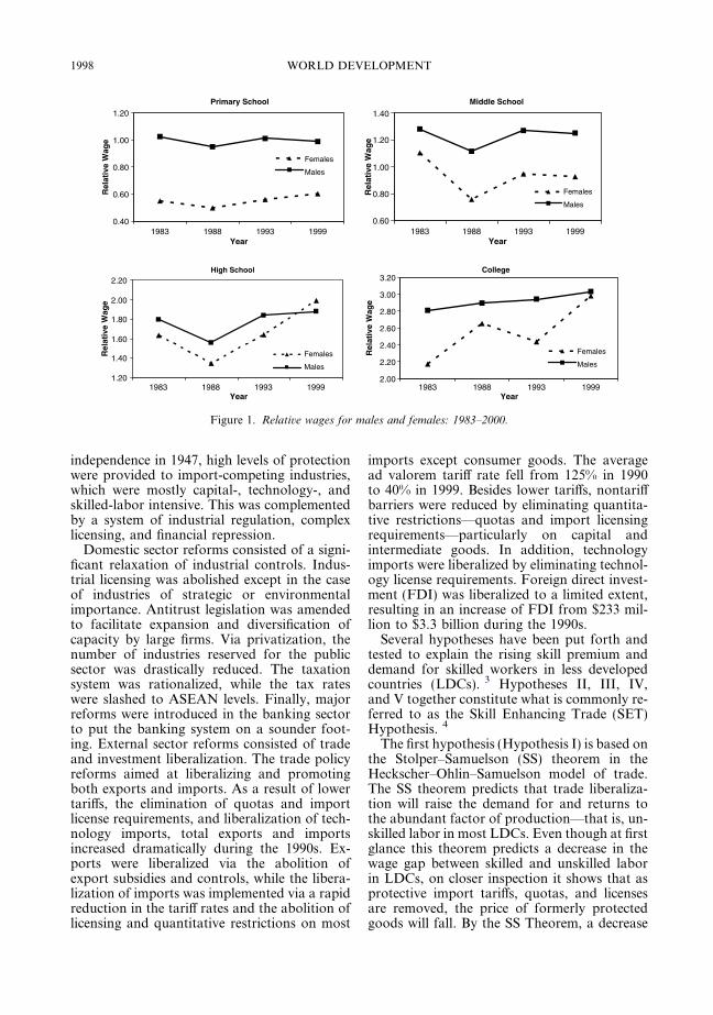
During the 1980s and 1990s, India experi-enced two dramatic changes in its wage struc-ture. First, there was a considerable wideningof the skill wage gap, accompanied by large in-creases in both the supply of and demand forhigh school and college graduates. Second, asFigure 1 shows, the gender wage differentialnarrowed considerably among high schooland college graduates. In examining alternativeexplanations for these changes, we find thatan increased demand for skilled workers andespecially for skilled women contributedsignificantly to these wage shifts. The skill-upgrading within industries was primarilyresponsible for these demand shifts. Since thesetwo decades mark a period of widespread eco-nomic liberalization in India, we measure thecontribution of external sector reforms to anoverall demand and find that internationaltrade-in manufactures benefited skilled menbut hurt skilled women, whereas trade-in ser-vices (outsourcing) benefited both male andfemale college graduates.

There is a vast literature that documentswage shifts and its determinants in the UnitedStates during the past few decades. 1 The liber-alization of trade and investment in severaldeveloping economies and increasing globaliza-

199

tion during this period suggests that a skill-abundant rich country, such as the UnitedStates, would experience a widening skill wagegap. The literature confirms this and finds thatthe relative demand shifted toward ‘‘skilled’’or ‘‘educated’’ workers and away from ‘‘un-skilled’’ or ‘‘uneducated’’ workers. The changesin technology and product demand that shiftedemployment away from manufacturing and to-ward sectors that are education and femaleintensive are offered as explanations for wageshifts in the United States.

In this paper, we focus on how economic lib-eralization and globalization affects the wagestructure in a poor but rapidly developing econ-omy that is abundant in unskilled labor. Indiaserves as a particularly interesting case studysince beginning in the mid-1980s, the Indiangovernment implemented a range of far-reach-ing economic policy reforms in the domesticand external sectors. 2 These reforms markeda clear break from the country’s socialist strat-egy of state-directed, heavy-industry based,and import substitution industrialization,which beginning in the early 1950s, was imple-mented through a series of five-year plans. Dur-ing the first three decades after India’s

7

Primary School

0.40

0.60

0.80

1.00

1.20

1983 1988 1993 1999Year

Rel

ativ

e W

age

Middle School

0.60

0.80

1.00

1.20

1.40

1983 1988 1993 1999Year

Rel

ativ

e W

age

High School

1.20

1.40

1.60

1.80

2.00

2.20

1983 1988 1993 1999Year

Rel

ativ

e W

age

Females

Males

Females

Males

College

2.00

2.20

2.40

2.60

2.80

3.00

3.20

1983 1988 1993 1999Year

Rel

ativ

e W

age

Females

Males

Females

Males

Figure 1. Relative wages for males and females: 1983–2000.

1998 WORLD DEVELOPMENT

independence in 1947, high levels of protectionwere provided to import-competing industries,which were mostly capital-, technology-, andskilled-labor intensive. This was complementedby a system of industrial regulation, complexlicensing, and financial repression.

Domestic sector reforms consisted of a signi-ficant relaxation of industrial controls. Indus-trial licensing was abolished except in the caseof industries of strategic or environmentalimportance. Antitrust legislation was amendedto facilitate expansion and diversification ofcapacity by large firms. Via privatization, thenumber of industries reserved for the publicsector was drastically reduced. The taxationsystem was rationalized, while the tax rateswere slashed to ASEAN levels. Finally, majorreforms were introduced in the banking sectorto put the banking system on a sounder foot-ing. External sector reforms consisted of tradeand investment liberalization. The trade policyreforms aimed at liberalizing and promotingboth exports and imports. As a result of lowertariffs, the elimination of quotas and importlicense requirements, and liberalization of tech-nology imports, total exports and importsincreased dramatically during the 1990s. Ex-ports were liberalized via the abolition ofexport subsidies and controls, while the libera-lization of imports was implemented via a rapidreduction in the tariff rates and the abolition oflicensing and quantitative restrictions on most

imports except consumer goods. The averagead valorem tariff rate fell from 125% in 1990to 40% in 1999. Besides lower tariffs, nontariffbarriers were reduced by eliminating quantita-tive restrictions—quotas and import licensingrequirements—particularly on capital andintermediate goods. In addition, technologyimports were liberalized by eliminating technol-ogy license requirements. Foreign direct invest-ment (FDI) was liberalized to a limited extent,resulting in an increase of FDI from $233 mil-lion to $3.3 billion during the 1990s.

Several hypotheses have been put forth andtested to explain the rising skill premium anddemand for skilled workers in less developedcountries (LDCs). 3 Hypotheses II, III, IV,and V together constitute what is commonly re-ferred to as the Skill Enhancing Trade (SET)Hypothesis. 4

The first hypothesis (Hypothesis I) is based onthe Stolper–Samuelson (SS) theorem in theHeckscher–Ohlin–Samuelson model of trade.The SS theorem predicts that trade liberaliza-tion will raise the demand for and returns tothe abundant factor of production—that is, un-skilled labor in most LDCs. Even though at firstglance this theorem predicts a decrease in thewage gap between skilled and unskilled laborin LDCs, on closer inspection it shows that asprotective import tariffs, quotas, and licensesare removed, the price of formerly protectedgoods will fall. By the SS Theorem, a decrease

ECONOMIC LIBERALIZATION AND WAGE INEQUALITY IN INDIA 1999

in the relative price of a good will decrease therelative price of the factor used intensively inthe production of that good and increase the rel-ative price of the other factor. Since in manyLDCs—namely, Colombia, Mexico, Brazil,and Morocco—the most protected sectors werethose that were intensive in unskilled labor, theSS theorem predicts that trade liberalization inthese countries should lower unskilled wages.India, on the other hand, had its highest protec-tion levels in human- and physical-capital-intensive sectors. Therefore, the rising demandfor and returns to skilled labor in India contra-dict the predictions of the SS theorem for thecountry—which are an increase in the demandfor and returns to unskilled labor and an expan-sion of unskilled-labor intensive sectors.

The second hypothesis (Hypothesis II) relatesto economic reforms in general and not specif-ically to trade liberalization in driving increaseddemand for and returns to skilled labor.According to this hypothesis, LDCs may expe-rience higher returns to skilled-labor intensiveoccupations—such as professional, managerial,and administrative jobs—as a result of reformsthat generate demand for individuals who canimplement these reforms. In India, reforms inboth the domestic and external sectors mayhave created more white-collar jobs. Theempirical evidence is mixed: Cragg and Epel-baum (1996) find support for this hypothesisfor pre-NAFTA Mexico while Attanasio,Goldberg, and Pavcnik (2004) find no changesin the occupational returns during 1986–98 inColombia.

Global production sharing or outsourcing isthe third hypothesis (Hypothesis III) that hasbeen provided to explain the rising skill pre-mium and demand for skilled labor in LDCs.Feenstra and Hanson (1996, 2003) argue thattrade and investment liberalization on the partof LDCs allows developed countries (DCs) totransfer the production of intermediate goodsand services to LDCs. For LDCs these activi-ties are skill intensive, which result in a greaterdemand for and returns to skilled labor. There-fore, the external sector reforms that promotetrade-in manufactures and services and thosethat attract foreign direct investment can bene-fit skilled workers in LDCs. Feenstra andHanson (1997) find empirical support for thishypothesis for the case of Mexico.

The fourth hypothesis (Hypothesis IV) re-lates skill-biased technical change (SBTC) toan increased demand for skilled labor and arising skill premium. Wood (1995) argues that

trade liberalization results in ‘‘defensive inno-vation’’—that is, greater competition from for-eign firms may induce domestic firms in LDCsto either engage in R&D or to adopt new andadvanced technologies in order to secure theirmarket share in the domestic and internationalmarkets. Because of technology-skill comple-mentarities, adoption of modern technologiesraises the demand for and returns to skilledlabor. Acemoglu (2003) describes how aftertrade liberalization in LDCs, increased capitalgoods imports can lead to a greater demandfor skilled workers as a result of capital-skillcomplementarities, thus increasing the skill pre-mium. An empirical support for this hypothesisis found by Attanasio et al. (2004) for Colom-bia and by Harrison and Hanson (1999) forthe case of Mexico. Gorg and Strobl (2002) findan increase in the relative wages of skilled laborin Ghana, brought about by skill-biased tech-nological change induced through imports oftechnology-intensive capital goods or exportactivity. However, Pavcnik (2003) rejects theSBTC hypothesis for Chilean plants.

Finally, the quality-upgrading of firms(Hypothesis V) is also considered a mechanismwhereby the demand for and returns to skilledlabor can increase in LDCs. The basic argu-ment is that trade liberalization may induce a‘‘quality’’ upgrading of firms, where qualitycan mean either firm productivity or productquality. Verhoogen (2004) finds a strong sup-port for this hypothesis for the case of Mexicowhere greater exports as a result of the pesocrisis resulted in better quality products beingproduced by exporters. Because higher qualityproducts require a higher proportion of skilledworkers, the relative demand for and returns toskilled labor increased.

Our analysis documents large overall demandshifts away from unskilled workers and towardskilled workers, which played an important rolein widening the skill wage gap during 1983–84and 1999–2000 in India. These demand shiftswere primarily within sectors—that is, skill-upgrading within industries explains most ofthe rising demand for skilled workers duringthis period in India. This result provides astrong evidence in the support of HypothesisII—that the creation of white-collar jobs as aresult of domestic and/or external sector re-forms played a major role in generating de-mand for skilled labor and increasing the skillpremium.

The agricultural sector experienced a dra-matic contraction, whereas manufacturing


employment fell slightly during the 1980s and1990s in India. On the other hand, the servicesector expanded considerably and was primar-ily responsible for generating a demand forhigh school and college graduates. This finding,along with the rising demand for and returnsto skilled labor, provide evidence to rejectHypothesis I. That a country abundant in un-skilled labor would experience these changesas its economy becomes increasingly liberal-ized, suggests that the SS theorem does nothold for the case of India. 5

In evaluating the role of external sector re-forms, we measure trade-induced demand shiftsin contributing to overall demand shifts in theeconomy. We find that trade-in manufacturesa generated demand for skilled men and adecreased demand for skilled women whereastrade-in services generated a demand for bothmale and female college graduates but a de-creased demand for men and women, withouta college degree. Because our trade-induced de-mand shifts arise from changes in the implicitlabor supply embodied in trade flows, we onlymeasure how overall changes in the skill con-tent of exports and imports result in changesin the demand for skilled and unskilled laborand cannot evaluate Hypotheses III, IV, andV separately. We therefore cannot attributeour trade-induced demand shifts to either thetransfer of manufacturing and service jobs fromDCs to India, defensive innovation, or qualityupgrading by firms. Being unable to distinguishbetween Hypotheses III, IV, and V is a limita-tion which we cannot address in this paperdue to the lack of appropriate data. Neverthe-less, the overall effects of India’s trade liberal-ization in manufacturing and services ondemand for skilled and unskilled labor providea valuable evidence by itself. That external sec-tor reforms have generated opportunities forskilled workers indicates that India’s economicliberalization has and can continue to createincentives for accumulating human capital,which is ultimately critical to the country’s eco-nomic development.

The rest of this paper is organized as follows.Section 2 describes the data used in our analy-sis. Section 3 documents the changes in relativewages in India during 1983–84 and 1999–2000.In Sections 4 and 5 we investigate the extentto which relative supply and demand changescontributed to shifts in relative wages in India.Section 6 measures the contribution of inter-national trade-in manufactures and servicestoward relative demand changes during

the 1980s and 1990s in India. Section 7 con-cludes.

2. DATA AND METHODOLOGY

The individual level data used in this studycomes from the Employment and Unemploy-ment Schedule of the National Sample SurveyOrganization (NSSO), administered nationallyby the Government of India. The Employmentand Unemployment Schedules are administeredapproximately every five years in four sub-rounds, each with a duration of three months.We use four rounds of the NSSO surveys thatcover the two decades that span India’s eco-nomic reforms—that is, 1983–84, 1987–88,1993–94, and 1999–2000. The NSSO surveyincludes household and individual leveldata—household size and composition, socialgroup, religion, income, assets, indebtedness,demographic variables (age, gender, maritalstatus), education participation and attain-ment, and a detailed employment section onprincipal and subsidiary activities (industry,occupation, type and amount of incomeearned, and intensity of each activity).

For our empirical analysis, we use data forindividuals aged 15 years and above and createtwo samples—a wage sample to measure hourlywages of workers by demographic group and acount sample to measure the amount of laborsupplied by these demographic groups. We di-vide our data into 100 distinct labor groups, de-fined by two gender groups (male and female),five education groups (less than primary, pri-mary, middle, high school, and college), and10 age groups (15–20, 20–25, 25–30, 30–35,35–40, 40–45, 45–50, 50–55, 55–60, and60+ years).

The wage measure we use throughout is theaverage hourly wage of workers within a gen-der–education–age cell. An individual’s averagehourly wage is computed as the total wagesduring the past week divided by the total hoursworked during that week. We then adjust theindividual wages to 1988 Rupees using state-level CPI for agricultural and industrial work-ers for rural and urban wages, respectively.This adjustment makes wages comparable overtime, across states, and across rural and urbansectors. Our wage sample includes regular wageand salary workers since wages are only re-ported for this group. Self-employed workers(both wage and nonwage earning) are excludedfrom our wage sample. The count sample in-


cludes all individuals who worked either asregular wage and salary workers or as self-employed workers (wage and nonwage earn-ing). 6 The amount of labor supplied by eachdemographic group is measured as the totalhours worked by each group as a proportionof the total hours worked by all groups in thatyear. The total hours worked by each group iscomputed as the sum of hours worked duringthe past week for all individuals within eachgender–education–age cell.

Rather than generate 100 labor groups forthe rural and urban sectors separately, ouranalysis aggregates both sectors. Even thoughrural–urban differences are potentially interest-ing, the reason for this aggregation is thescarcity of data (especially for wages during1987–88) which results in the missing valuesfor some cells. Since the NSSO data reportswages only for individuals who earn a regularwage or salary, wages are missing for a consid-erable number of individuals in the rural sector,making it necessary to aggregate both sectorsfor our analysis.

We calculate relative wages, a (100 · 4) ma-trix Wr, and relative supply, a (100 · 4) matrixXr, from our wage and count samples. Ourwage data consists of a (100 · 4) matrix W,which consists of the average hourly wage (ad-justed to 1988 Rupees) from the wage samplefor each of the 100 demographic groups in eachof four years. Our labor supply data consists ofa (100 · 4) matrix X, which consists of the pro-portion of hours worked from the count samplefor each of the 100 demographic groups in eachof four years. From X we construct a 100-element vector, N, of the average employmentshares of each group over the four years. Weuse this vector of fixed weights to constructwage indices for each year as N 0W, a (1 · 4)matrix. Deflating wages in each year (W) bythe value of the wage index for that year(N 0W) generates the relative wages for eachdemographic group in each year, denoted bya (100 · 4) matrix Wr.

7

From Wr we calculate a 100-element vector,X, of average relative wages of each group overthe four years. The average of the relativewages of each demographic group over the fouryears provides a natural basis for aggregatingquantities of labor supplied across groups interms of efficiency units. We weigh the employ-ment share of each group (X) by the averagerelative wage of that group (X) and sum overall groups to construct a measure of the totallabor supply in the economy in each year in effi-

ciency units, X 0X, a (1 · 4) matrix. We then de-flate the actual labor supply (X) by the totallabor supply in the economy measured in effi-ciency units (X 0X) for each demographic groupin each year to get a (100 · 4) relative supplymatrix Xr.

8

3. SHIFTS IN RELATIVE WAGES

Table 1 reports changes in average relativehourly wages for all workers, women, andmen by education levels over four periods inIndia—that is, three sub-periods 1983–88,1987–94, and 1993–2000 and the overall period1983–2000. The average hourly wages are rela-tive wages—that is, each group’s wage relativeto the wages for a fixed bundle of workers—described in Section 2 and calculated from the(100 · 4) matrix Wr. The figures in Table 1 rep-resent changes in the log relative wage, multi-plied by 100, for each group over the relevanttime period.

For the period during 1983–2000, the relativewages of all workers (both men and women to-gether) with less than primary, primary, highschool, and college education increased whilethose of workers with middle schooling de-creased. The decline in the relative wages ofworkers with middle schooling was large witheven larger increases in the relative wages ofhigh school and college graduates. We observethis same pattern in the relative wages of womenduring 1983–2000. The relative wages of allwomen except those with middle schooling in-creased, with a substantial decrease in the rela-tive wages of women with middle schoolingand large increases in the relative wages of highschool and college female graduates. For men,we observe decreases in the relative wages ofworkers with less than primary, primary, andmiddle schooling and increases in the relativewages of high school and college male graduates.

The rise in the relative wages of less-skilledwomen can be explained by the SS theorem.On the other hand, the fall in the relative wagesof less-skilled men together with the rise inthe relative wages of skilled women and mensuggest that the SET Hypothesis might haveplayed a dominant role during the period ofIndia’s reforms. Can we attribute the increasein the relative earnings of skilled workers tofirms’ higher demand for skilled labor? More-over, if relative demand shifts can explain thewidening skill wage gap and the narrowinggender wage gap for high school and college

Table 1. Shifts in relative wages in India: 1983–2000

Group Change in log relative wages (multiplied by 100)

1983–88 1987–94 1993–2000 1983–2000

All adults

<Primary school 23.34 �19.91 �1.82 1.61(0.0309) (0.0304) (0.0240) (0.0246)

Primary school �8.35 8.16 1.28 1.09(0.0418) (0.0418) (0.0430) (0.0434)

Middle school �24.16 16.85 �1.76 �9.07(0.0617) (0.0668) (0.0701) (0.0653)

High school �16.62 18.10 10.75 12.23(0.0707) (0.0920) (0.1115) (0.0946)

College 10.77 �3.13 11.15 18.79(0.1795) (0.1886) (0.1591) (0.1483)

Women

<Primary school 39.08 �30.99 �1.26 6.83(0.0253) (0.0252) (0.0045) (0.0049)

Primary school �9.82 11.70 7.48 9.36(0.0215) (0.0197) (0.0204) (0.0222)

Middle school �37.58 22.30 �2.14 �17.42(0.0656) (0.0678) (0.0725) (0.0704)

High school �19.31 19.81 19.26 19.76(0.0586) (0.0958) (0.1193) (0.0921)

College 19.95 �8.53 20.15 31.56(0.1446) (0.1635) (0.1524) (0.1319)

Men

<Primary school 13.71 �12.88 �2.14 �1.32(0.0214) (0.0221) (0.0157) (0.0148)

Primary school �7.57 6.25 �2.32 �3.64(0.0290) (0.0323) (0.0401) (0.0375)

Middle school �13.89 12.96 �1.47 �2.41(0.0534) (0.0594) (0.0628) (0.0572)

High school �14.24 16.60 2.47 4.83(0.0821) (0.0909) (0.1083) (0.1011)

College 3.04 1.58 3.03 7.65(0.2111) (0.2159) (0.1697) (0.1636)

The reported numbers are of the form D(log Wr) · 100, where Wr represents relative wages. Figures in parentheses

are standard errors of the difference in relative wages between years t and t 0. These are calculated as SEtt0 ¼ffiffiffiffiffiffiffiffiffiffiffiffiffis2

tntþ s2

t0nt0

r,

where st is the standard deviation of relative wages in year t and nt is the number of observations in year t, and t 0 > t.


graduates, how has India’s trade liberalizationcontributed toward these demand shifts? Wenow turn to answering these questions.

4. ALTERNATIVE EXPLANATIONS FORRELATIVE WAGE SHIFTS

The previous section documented large shiftsin the relative wages among women and menduring the 1980s and 1990s in India. WhileIndia’s trade liberalization could be responsiblefor these changes by altering the relative de-

mand for workers with different education orskill levels, other factors—namely relative sup-ply shifts and changes in wage legislation—could have brought about these changes aswell. We investigate relative supply and de-mand changes as potential determinants ofthe relative wage shifts in India.

(a) Changes in relative labor supply

Table 2 summarizes changes in the relativelabor supply over the 1983–2000 period, whereeach group’s supply is measured in efficiency

Table 2. Relative supply changes: 1983–2000

Group Change in log relative supply (multiplied by 100)

1983–88 1987–94 1993–2000 1983–2000

All adults

<Primary school �21.70 �13.73 �16.60 �52.03(0.0017) (0.0013) (0.0012) (0.0016)

Primary school �3.83 �21.22 �13.01 �38.06(0.0010) (0.0008) (0.0007) (0.0009)

Middle school 1.30 2.91 5.57 9.77(0.0010) (0.0010) (0.0009) (0.0010)

High school 18.07 14.08 10.65 42.79(0.0009) (0.0010) (0.0011) (0.0010)

College 33.70 14.25 8.75 56.69(0.0004) (0.0005) (0.0006) (0.0005)

Women

<Primary school �11.00 �15.88 �14.67 �41.56(0.0009) (0.0007) (0.0006) (0.0008)

Primary school 4.58 6.43 �4.89 6.12(0.0002) (0.0002) (0.0002) (0.0002)

Middle school 27.42 31.16 17.44 76.03(0.0001) (0.0001) (0.0002) (0.0001)

High school 26.62 30.58 14.02 71.22(0.0001) (0.0001) (0.0002) (0.0001)

College 52.87 17.61 9.64 80.12(0.0001) (0.0001) (0.0001) (0.0001)

Men

<Primary school �27.30 �12.53 �17.68 �57.51(0.0009) (0.0008) (0.0008) (0.0009)

Primary school �5.02 �26.05 �14.75 �45.82(0.0008) (0.0006) (0.0005) (0.0007)

Middle school �0.88 �0.27 3.90 2.75(0.0010) (0.0009) (0.0008) (0.0009)

High school 17.24 12.25 10.23 39.72(0.0009) (0.0009) (0.0010) (0.0010)

College 30.85 13.68 8.59 53.12(0.0005) (0.0006) (0.0006) (0.0005)

The reported numbers are of the form D(log Xr) · 100, where Xr represents relative supply. Figures in parentheses are

standard errors of the difference in relative supply between years t and t 0. These are calculated as SEtt0 ¼ffiffiffiffiffiffiffiffiffiffiffiffiffis2

tntþ s2

t0nt0

r,

where st is the standard deviation of relative supply in year t and nt is the number of observations in year t, and t 0 > t.


units and includes all workers in the count sam-ple. Each group’s supply is then measured rela-tive to the total supply in efficiency units in agiven year. The figures in Table 2 representchanges in the log relative supply, multipliedby 100, for each group over the relevant timeperiod. For the 1983–2000 period, the relativesupplies of all workers (both men and womentogether) with less than primary and primaryeducation declined considerably and those ofworkers with middle, high school, and collegeeducation rose substantially. We observe an

identical pattern for men—that is, large de-creases in the relative supplies of men with lessthan primary and primary education, a smallincrease in the relative supply of men with mid-dle schooling, and substantial increases in therelative supplies of high school and collegemale graduates. While the relative supply ofwomen with less than primary education de-clined considerably, the relative supplies ofwomen with primary schooling rose slightly,while those of middle, high school, and collegeeducated women rose substantially.


Table 2 documents a trend toward rising edu-cation levels during the 1980s and 1990s inIndia, which could be the result of educationalpolicies such as higher public expenditure oneducation, more schools, better accessibility toschools, higher quality of education, and otherincentives such as provision of meals in schools.

(b) Changes in relative labor demand

Changes in the demand for labor with differ-ent education levels can result from changes inthe sectoral composition of output, which canbe attributed primarily to changes in the prod-uct demand. In Table 3 we define 18 industriesand three occupation groups, while Table 4 re-ports average industry and occupation distribu-tions for five education groups each for menand women. The figures for each gender–educa-tion group represent the share of employment(measured in hours worked during the preced-ing week) of that gender–education group inthe corresponding industry or occupation aver-aged over the four survey years. The largedifferences in employment shares by gender–

Table 3. Industry and

Industry/occupation

Industry

1 Agriculture, hunting2 Mining and quarryin3 Manufacture of food4 Manufacture of text5 Manufacture of woo6 Manufacture of pap7 Manufacture of chem8 Manufacture of non9 Manufacture of basi10 Manufacture of mac11 Other manufacturin12 Electricity, gas, stea13 Construction14 Wholesale trade, ret15 Transport, commun16 Storage, warehousin17 Financing, insurance18 Community, social,

Occupation

1 Professional, technic2 Clerical and sales w3 Production and serv

Industry 4 includes cotton, wool, silk, manmade and synOccupation category 3—that is, production and service worelated workers.

education groups suggest that shifts in labordemand across industries and occupationsshould have a significant effect on the relativewages of these groups.

While industry groups cannot be classified asexclusively low-, medium-, or high-skill becauseof varying education levels of its workers, it ispossible to divide occupations into three skillgroups. High-skill occupations include pro-fessional, technical, administrative, executive,and managerial workers; medium-skill occupa-tions consist of clerical and sales workers; andlow-skill occupations include production andservice workers. Table 5 shows employmentshifts into high- and medium-skill occupa-tions during 1983–2000—that is, the share ofworkers employed in professional, technical,administrative, executive, and managerial occu-pations increased by 5.28% points, while that ofclerical and sales workers rose by 2.06% points.During the same period there was an employ-ment shift out of low-skill occupations—thatis, a decrease of 7.34% points in the share ofworkers employed in production and serviceoccupations. Table 5 demonstrates that skilled

occupation groups

, forestry, and fishingg, beverage, and tobacco products

iles, leather, fur, wearing apparel, and footweard and wood productser, paper products, printing, and publishing

icals, rubber, plastic, petroleum, and coal productsmetallic mineral productsc metals, metal products, and metal partshinery and transport equipment and parts

g industriesm, water works, and water supply

ail trade, restaurants, and hotelsicationsg, repair services, real estate, business servicespersonal services, except repair services

al, administrative, executive, and managerial workersorkersice workers

thetic fiber, and jute and other vegetable fiber textiles.rkers—includes farmers, fishermen, hunters, loggers, and

Table 5. Changes in industry and occupation distributions: 1983–2000

Industry/occupation Change in employment share(in percentage points)

1983–88 1987–94 1993–2000 1983–2000

Agriculture, hunting, forestry, and fishing �2.31 �1.95 �4.15 �8.41Mining and quarrying �0.21 0.30 �0.17 �0.07Manufacture of food, beverage, and tobacco products �0.16 0.09 0.17 0.10Manufacture of textiles, leather, fur, wearing apparel, and

footwear0.24 �1.58 0.15 �1.18

Manufacture of wood and wood products 0.05 �0.21 �0.06 �0.23Manufacture of paper, paper products, printing, and publishing 0.05 �0.06 0.07 0.06Manufacture of chemicals, rubber, plastic, petroleum, and coal

products0.09 0.10 0.08 0.27

Manufacture of nonmetallic mineral products �0.10 �0.10 0.13 �0.07Manufacture of basic metals, metal products, and metal parts 0.12 �0.13 0.12 0.12Manufacture of machinery and transport equipment and parts 0.14 �0.13 �0.01 0.00Other manufacturing industries 0.09 0.06 0.25 0.40Electricity, gas, steam, water works, and water supply �0.01 0.08 �0.06 0.01Construction �0.32 0.67 0.94 1.29Wholesale trade, retail trade, restaurants, and hotels 2.36 �0.78 2.06 3.63Transport, communications �0.18 0.36 0.67 0.85Storage, warehousing, repair services 0.57 0.31 0.78 1.66Financing, insurance, real estate, business services �0.41 2.95 �1.13 1.41Community, social, personal services, except repair services 0.01 0.00 0.16 0.16

Professional, technical, administrative, executive, and managerialworkers

1.49 1.33 2.46 5.28

Clerical and sales workers 2.22 �0.31 0.14 2.06Production and service workers �3.72 �1.02 �2.60 �7.34

Table 4. Average industry and occupation distributions for men and women: 1983–2000

Industry/occupation

Women education level Men education level

<Primary Primary Middle High College <Primary Primary Middle High College

1 27.31 1.81 0.59 0.15 0.02 49.09 10.55 6.98 3.05 0.442 15.69 0.82 0.08 0.45 0.16 52.76 9.50 9.53 8.35 2.673 28.32 4.88 1.22 0.46 0.04 32.63 13.11 9.36 8.00 1.974 15.82 3.74 2.26 1.00 0.13 35.87 18.62 13.07 7.78 1.715 14.11 1.60 0.38 0.00 0.08 46.88 19.31 11.90 5.10 0.646 6.00 2.24 2.17 2.79 0.12 15.34 17.72 22.04 22.65 8.927 9.04 3.63 1.41 1.43 0.44 17.13 14.60 16.82 20.26 15.248 21.05 0.71 0.34 0.28 0.08 51.48 11.27 7.72 5.26 1.819 2.64 0.38 0.33 0.33 0.27 37.04 16.32 19.82 16.51 6.3610 1.03 0.44 0.29 1.12 0.59 22.03 15.56 16.81 30.70 11.4211 9.41 1.87 0.69 0.50 0.00 29.38 23.42 20.08 11.01 3.6412 0.72 0.11 0.07 0.98 1.32 21.12 16.20 21.96 26.04 11.5013 12.94 0.57 0.22 0.15 0.08 52.56 14.64 9.65 6.76 2.4114 9.26 1.22 0.68 0.32 0.08 30.34 18.90 19.02 15.79 4.4015 1.23 0.20 0.15 0.69 0.47 39.90 17.58 17.50 17.41 4.8516 1.05 0.14 0.27 0.53 1.65 20.87 14.52 17.73 20.84 22.4017 10.98 1.43 1.52 5.01 3.37 18.45 9.56 12.74 22.85 14.1018 11.59 0.00 0.00 0.00 1.49 29.57 9.81 15.45 16.64 15.45

1 2.88 0.70 1.84 6.95 5.25 8.87 7.03 11.29 28.73 26.472 6.51 0.81 0.62 1.44 0.92 22.01 14.87 17.92 24.35 10.563 22.32 1.81 0.65 0.22 0.03 47.61 12.81 9.25 4.64 0.67



jobs (those employing high school and collegegraduates) in professional, technical, adminis-trative, executive, and managerial occupations(occupation category 1) are dominated bymen (28.73% and 26.47%, respectively) ratherthan women (6.95% and 5.25%, respectively).This suggests that employment shifts intohigh-skill occupations may have disproportion-ately benefited high-skilled men rather thanhigh-skilled women.

The actual employment levels and changesare determined by the interaction of both thedemand for and supply of different laborgroups. However, if changes in India’s occupa-tion distribution can be considered a roughmeasure of shifts in firms’ demand for workerswith different education levels, these occupa-tional shifts show a simultaneous increase inthe demand for high-skilled workers and de-crease in the demand for medium- and low-skilled workers, suggesting that the SETHypothesis might have played a significant roleduring India’s reforms.

5. NONPARAMETRIC ANALYSIS

The nonparametric methodology proposedby Katz and Murphy (1992) provides a simpleframework for decomposing the extent towhich relative supply and demand changes con-tributed to the relative wage changes in India.We first test whether relative labor supplychanges alone can explain changes in the rela-tive wages by education levels, or, instead, rela-tive labor demand changes must have beennon-neutral or factor biased. We then evaluatebetween- and within-sector changes in relativelabor demand.

(a) Relative supply versus relative demandchanges

If we assume a stable relative demand for ourlabor groups, the relative supply shifts pre-sented in Table 2 cannot explain the relativewage shifts observed during the 1983–2000period for most groups. With a stable relativedemand, we should observe a negative correla-tion between the changes in relative suppliesand wages. We observe this negative correla-tion for only two groups during the 1983–2000 period—that is, all workers and men withprimary education. For all other groups thiscorrelation is positive, implying that the rela-tive demand for these groups must have chan-

ged during this period. Using our measuresfor relative wages (Wr) and relative supply(Xr), we first test whether relative labor supplychanges alone can explain the changes in rela-tive wages by education levels, or, instead, rela-tive labor demand changes must have beennon-neutral or factor biased.

In the Katz and Murphy (1992) framework,the aggregate production function consists ofK types of labor inputs. 9 The vector of associ-ated labor demands can be written as

X t ¼ DðW t; ZtÞ; ð1:1Þwhere Xt is a (K · 1) vector of labor inputs em-ployed in the market in year t, Wt is a (K · 1)vector of market prices for these inputs in yeart, and Zt is a (K · 1) vector of demand shiftvariables in year t. The demand shift variablesin Zt embody the effects of technology, othernonlabor inputs such as capital, and productdemand on the demand for labor inputs.

Eqn. (1.1) can be written in terms of differen-tials as

dX t ¼ Dw dW t þ Dz dZt: ð1:2ÞUnder the assumption that the aggregate pro-duction function is concave, the (K · K) matrixof cross-price effects Dw is negative semi-defi-nite which implies that

dW 0tðdX t � Dz dZtÞ ¼ dW 0

tDw dW t 6 0 ð1:3Þ

which says that the changes in factor supplies(dXt) net of demand shifts (Dz dZt) and thechanges in wages (dWt) must negatively co-vary. We can therefore test whether or notsupply shifts alone can explain the changes inrelative wages. If factor demand is stable (i.e.,Zt is fixed or dZt = 0) then Eqn. (1.3) impliesthat dW 0

t dX t 6 0. If we compare two years sand t, and find that

ðW t �W sÞ0ðX t � X sÞ 6 0; ð1:4Þ

then the observed changes in relative wages canpotentially be explained solely by supply shifts.In other words, if the inequality in Eqn. (1.4)holds then the period between years s and tcould have experienced a fixed factor demandwhich would have had no impact on relativewages. If the inequality in Eqn. (1.4) does nothold, then supply shifts alone cannot explainthe relative wage changes. Instead, non-neutralor factor-biased demand shifts must also haveplayed a role in explaining relative wagechanges.


We test the stable relative demand hypothesisby computing the inner products of changes inrelative wages and the changes in relative sup-plies for the 100 gender–education–age groups(Wt � Ws)

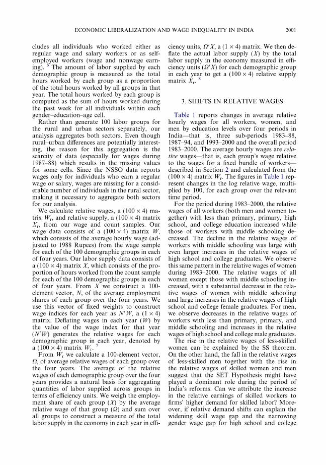
0(Xt � Xs) for our four time periods.The results are presented in Table 6, wherethree of the four comparisons are positive andtherefore reject a stable relative demandhypothesis. During 1983–88 there is a possibil-ity that relative demand was stable and there-fore did not affect relative wages. For allother periods, we find that shifts in the relativedemand played an important role in the relativewage changes in India. The positive relation-ship between the changes in relative wagesand relative supplies is the strongest for theoverall period 1983–2000 (0.0218) with thesub-period 1987–94 being the largest (0.0170)of the three sub-periods.

Figure 2 illustrates our results by plotting thechanges in log relative wages against changes inlog relative supplies for the 100 labor groupsfor each of the four periods. The lines drawnin the figures are predicted values from theweighed least squares regressions of changesin log relative wages on the changes in logrelative supplies for each time period, usingemployment shares of each group in the initialperiod as weights. The graphs for the three sub-periods 1983–88, 1987–94, and 1993–2000 re-inforce our findings from the inner products,showing a strong negative relationship in rela-tive supplies and wages during 1983–88, astrong positive relationship during 1987–94,and a weak relationship during 1993–2000.Even though the inner product for the overallperiod 1983–2000 is positive, the graph forthis period shows a weak relationship betweenrelative supplies and wages.

(b) Between- and within-sector demand changes

To explore the role of relative demandchanges in relative wage changes, we focuson two types of demand changes—those that

Table 6. Relationship between changes in relative w

1983–88 198

Inner product �0.0289 0.0Coefficient �0.6157*** 0.4Standard error (0.1592) (0.2

The reported numbers for inner products are the inner prodsupplies. The coefficient estimates and standard errors aresupplies, using employment shares of each group in the incoefficients that are significant at the 10% and 1% levels re

occur between industries (shifts that change theallocation of labor demand between industriesat fixed relative wages) and those that occurwithin industries (shifts that change the alloca-tion of labor demand within industries at fixedrelative wages). Important sources of both be-tween- and within-sector demand changes in-clude skill-biased technology transfer, changesin the prices of nonlabor inputs such as capital,changes in product demand, and changes inthe composition of domestic output.

The between- and within-sector demand shiftmeasures proposed by Katz and Murphy (1992)are based on the fixed coefficients manpowerrequirements index (Freeman, 1980). This indexmeasures the percentage change in the demandfor a demographic group as the weighted aver-age of the percentage employment growth byindustry, where the weights are the industrialemployment distribution for the demographicgroup in a base period. The index can be writtenas

DX dk ¼

Xj

Ejk

Ek

� �DEj

Ej

� �¼P

jajkDEj

Ek; ð1:5Þ

where k indexes demographic groups and j in-dexes sectors. DX d

k is the change in demandfor group k, Ej is the total labor input in sectorj, DEj is the change between years of total laborinput in sector j, Ek is the base year employ-ment of group k, and ajk ¼ Ejk

Ejis the group k’s

share of total employment in sector j in the baseperiod. The employment measures Ek and Ej

are in efficiency units. 10 We turn Eqn. (1.5)into an index of relative demand shifts by nor-malizing the employment measures Ek and Ej

so that the total employment in efficiency unitsin each year sums to one. We use the average ofthe four survey years to be our base period.Thus, we use the average share of total employ-ment in sector j of group k over the 1983–2000period as our measure of ajk and the averageshare of group k in total employment over the1983–2000 period as our measure of Ek.

ages and changes in relative supplies: 1983–2000

7–94 1993–2000 1983–2000

170 0.0031 0.0218471* 0.0461 0.0147310) (0.0435) (0.0270)

ucts of changes in relative wages and changes in relativefrom regressions of log relative wages on log relative

itial period as weights. A * and *** represent regressionspectively.

-1-.

50

.51

lnw

8388

/Fitt

ed v

alue

s

-1 -.5 0 .5 1lnx8388

-1.5

-1-.

50

.51

lnw

8794

/Fitt

ed v

alue

s

-.5 0 .5 1lnx8794

lnw8794 Fitted values

-.5

0.5

11.

5ln

w93

00/F

itted

val

ues

-.4 -.2 -5.55e-17 .2 .4 .6lnx9300


-1-.

50

.51

lnw

8300

/Fitt

ed v

alue

s

-1 -.5 0 .5 1 1.5lnx8300



Figure 2. Wage and supply changes for 100 groups: 1983–2000.


We use Eqn. (1.5) to calculate overall, be-tween, and within sector demand shifts basedon employment in 18 industries and three occu-pations (defined in Table 3). We define our over-all (industry-occupation) demand shift index forgroup k, DX d

k , as the index given in Eqn. (1.5)when j indexes our 48 industry-occupation cells.We also decompose this index into between-and within-industry components. The between-industry demand shift index for group k, DX b

k ,is the index given in Eqn. (1.5) when j indexesthe 18 industries. The within-industry demandshift index for group k, DX w

k , is calculated asthe difference between the overall demand shiftindex and the between-industry demand shiftindex (i.e., DX w

k ¼ DX dk � DX b

k). The within-industry demand shifts reflect shifts in employ-ment among occupations within industries.

Table 7 reports the relative demand shift esti-mates for 10 demographic groups over six timeperiods. During 1983–2000, between-sector,within-sector, and overall demand shifted awayfrom men and women with less than primary,primary, and middle schooling in favor ofmen and women with high school and collegeeducation. Between-sector shifts are substan-tially smaller than within-sector shifts for all

demographic groups, indicating that whilethere was some expansion of sectors employingmore educated labor and contraction of sectorsemploying less educated labor, overall shifts inrelative demand were caused primarily by skill-upgrading within industries—that is, shiftsaway from low-skill occupations and towardhigh-skill occupations within industries. Theoccupational shifts reported in Table 5 supportthis finding for the 1983–2000 period. 11 Thesewithin-sector shifts in favor of skilled laborsupport Hypothesis II—that is, the creation ofwhite-collar jobs as a result of domestic and/or external sector reforms raised a demandfor more educated labor.

In order to identify how various sectorscontributed toward the overall demand shiftspresented in Table 7, we calculate the disaggre-gated demand shift measures for three broadsectors—agriculture, manufacturing, and ser-vices. Table 8 shows that the decline in therelative demand for uneducated and less edu-cated men and women is dominated by theagricultural sector. However, the increase inthe relative demand for high school and collegeeducated men and women, is driven by the ser-vice sector. These results imply that during the

Table 7. Sector and occupation based relative demand shifts: 1983–2000

Group Change in log relative demand (multiplied by 100)

1983–88 1987–94 1993–2000 1983–2000

Between sector shift

Women<Primary school �2.05 �2.55 �2.76 �7.81Primary school �0.89 �2.74 �1.58 �5.41Middle school �0.01 �0.69 �1.04 �1.76High school �0.87 4.63 �2.41 1.64College �0.45 6.72 �2.14 4.49

Men<Primary school �1.32 �2.56 �0.81 �4.85Primary school �0.08 �2.02 0.62 �1.46Middle school 0.07 �1.18 0.47 �0.62High school 0.71 1.03 0.78 2.48College 1.42 2.95 1.12 5.30

Within sector shift

Women<Primary school �6.90 �3.33 �8.48 �20.82Primary school �5.35 �3.71 �6.97 �17.52Middle school �2.74 �1.15 �3.22 �7.36High school 0.82 6.34 �1.09 6.15College 4.42 9.19 3.03 15.54

Men<Primary school �6.57 �3.17 �5.35 �16.38Primary school �4.28 �2.69 �2.73 �10.15Middle school �2.91 �1.70 �3.19 �8.06High school 1.86 1.07 1.03 3.86College 9.43 5.49 8.24 21.00

Overall shift (industry and occupation)

Women<Primary school �8.96 �5.88 �11.23 �28.63Primary school �6.25 �6.45 �8.55 �22.93Middle school �2.76 �1.84 �4.26 �9.12High school �0.05 10.97 �3.50 7.79College 3.97 15.90 0.89 20.03

Men<Primary school �7.89 �5.73 �6.15 �21.23Primary school �4.36 �4.72 �2.11 �11.61Middle school �2.84 �2.88 �2.72 �8.69High school 2.57 2.10 1.81 6.34College 10.84 8.45 9.36 26.30

The reported numbers are of the form log 1þ DX sk

� �� 100, where s represents between sector (b), within-sector (w),

and overall (d) demand.


1980s and 1990s India’s economy movedaway from agriculture and toward services,generating lower demand for unskilled laborand higher demand for skilled labor. The con-traction of agriculture and expansion ofservices, together with increased demand for

skilled workers is a strong evidence againstHypothesis I. The liberalization of the domesticand external sectors in India appears to haveshifted employment away from unskilled-laborintensive and toward skilled-labor-intensiveactivities.

Table 8. Relative demand shifts in agriculture, manufacturing, and services: 1983–2000

Group Change in log relative demand (multiplied by 100)

1983–88 1987–94 1993–2000 1983–2000

Overall demand shift in agriculture

Women<Primary school �6.97 �6.04 �10.19 �25.21Primary school �5.10 �4.18 �6.38 �16.55Middle school �2.79 �2.24 �3.14 �8.41High school �0.51 �0.51 �0.43 �1.46College �0.13 �0.07 0.34 0.14

Men<Primary school �5.75 �4.94 �8.21 �20.19Primary school �3.48 �2.98 �4.75 �11.65Middle school �3.47 �3.00 �4.74 �11.64High school �1.34 �1.22 �1.33 �3.94College �0.69 �0.53 0.10 �1.13

Overall demand shift in manufacturing

Women<Primary school �0.65 �1.87 �0.09 �2.63Primary school �0.94 �3.97 0.07 �4.87Middle school �0.35 �3.41 �0.15 �3.92High school 0.70 �1.29 0.21 �0.37College 1.12 �0.55 0.36 0.93

Men<Primary school �0.38 �3.18 �0.07 �3.66Primary school �0.01 �4.13 0.11 �4.02Middle school 0.22 �3.20 0.38 �2.58High school 1.62 �2.17 0.85 0.35College 3.69 �1.01 1.07 3.76

Overall demand shift in services

Women<Primary school �0.83 1.88 �0.83 0.25Primary school �0.05 1.82 �1.03 0.77Middle school 1.09 3.73 0.53 5.29High school �0.07 12.47 �2.83 9.91College 2.79 15.96 0.22 18.53

Men<Primary school �0.83 1.94 2.03 3.12Primary school �0.30 2.34 2.18 4.19Middle school 0.41 2.92 1.16 4.44High school 2.09 5.05 0.98 7.95College 7.11 9.22 6.75 21.52

The reported numbers are of the form log 1þ DX sk

� �� 100, where s represents between sector (b), within-sector (w),

and overall (d) demand.


6. DEMAND SHIFTS ARISING FROMINTERNATIONAL TRADE

The occurrence of a widening wage differen-tial between unskilled and skilled workers, to-

gether with large increases in the demand forskilled workers during the two decades thatspan India’s economic reforms suggest thatthe SET Hypothesis might have played a roleas a result of trade liberalization. In this section


we examine the extent to which internationaltrade in manufactured goods and services con-tributed to relative demand shifts during the1980s and 1990s in India. Following Katz andMurphy (1992) we estimate the labor supplyequivalents of trade (i.e., the implicit labor sup-ply embodied in trade) by transforming tradeflows into labor supply equivalents on the basisof the utilization of labor inputs in the domesticmanufacturing industries. We measure only thedirect labor supply embodied in trade andignore the input–output effects. Therefore, theimplicit labor supply in trade is the labor inputrequired to produce traded output domesti-cally.

This section essentially utilizes the factor con-tent approach to measure the impact of trade onwages. As documented by Wood (1995), thisapproach has several major drawbacks accord-ing to Leamer (1994) but may nevertheless bethe appropriate method of analysis due to datalimitations. The major criticism is that tradeaffects wages only through prices, making itunnecessary to focus on the factor content intrade flows. Also, trade flows are a functionof wages and therefore endogenous. Giventhese problems, a more appropriate empiricalanalysis would be to examine how plausiblyexogenous industry tariffs affect the demandfor skilled and unskilled labor. This wouldallow us to estimate the causal impacts oftrade liberalization on relative demand usingtrade prices rather trade flows as the measureof trade reform.

Despite the advantages of using tariffs ratherthan trade flows, we use the factor content ap-proach in our analysis because even thoughdata on tariffs is available at a reasonable levelof industry disaggregation, such an analysiswould require detailed firm-level or industry-level data. Estimating the impact of industry-level tariffs on demand for skilled and unskilledlabor at the firm or industry level within thecontext of a regression requires informationon the employment of skilled and unskilledlabor at the firm or industry level. To the bestof our knowledge, such data is available inthe Annual Survey of Industries but only fora few years during the 1980s, which does notencompass the period of India’s external liber-alization, making it inappropriate for ourempirical analysis. An alternative method ofanalysis is to estimate the impact of tariffs di-rectly on the industry wages for skilled and un-skilled men and women, as in Dutta (2004),Reilly and Dutta (2005), and Kumar and Mis-

hra (2005) who use the same NSSO data aswe do in this analysis. This direct approach ismore informative and robust if the aim is toestimate the direct impact of trade liberaliza-tion on wage inequality and not distinguish be-tween supply-side and demand-side factors inshifting wages. The focus of this section is toestimate the impact of external sector reformson relative demand shifts not on wage inequal-ity, making the factor content approach moreappropriate and the only one given the datalimitations.

We measure Lkt , the implicit labor supply of

demographic group k embodied in trade in yeart as

Lkt ¼

Xi

eki Eit

I it

Y it

� �� ; ð1:6Þ

where i indexes 16 manufacturing industries, kindexes 10 demographic groups (two genderand five education groups), and t indexes fouryears. ek

i is the average proportion of employ-ment in industry i among workers in groupk over the 1983–2000 period, Eit is the shareof employment in industry i in year tP

iEit ¼ 1� �

, Iit is the net imports in industry iin year t (Importsit � Exportsit), and Yit is theoutput in industry i in year t. Positive net im-ports imply that the country is importing moreforeign labor than exporting domestic labor,which will result in a fall in domestic labor de-mand. 12

We measure T kt , the effect of trade on relative

demand for group k in year t as

T kt ¼ �

1

Ek

� �Xi

eki Eit

I it

Y it

� �� þX

i

EitI it

Y it

� �;

ð1:7Þwhere Ek is the average share of total emp-loyment of group k during the 1983–2000period. 13 The first term in Eqn. (1.7) is the im-plicit labor supply of group k embodied intrade, normalized by base year employment ofgroup k (Ek) with the sign reversed to convertthe supply shift measure into a demand shiftmeasure. The second term adjusts the demandshift measure so that trade affects only relativedemands for labor. 14 We use data on imports,exports, and output by industry for the years1983, 1988, 1993, and 1999 from the Trade &Production Database, provided by the WorldBank. These data cover 3-digit ISIC manufac-turing industries, which we aggregate into 16industry groups, as shown in Table 9.

Table 9. Classification of manufacturing industries

ISIC code Industry

1 311 Manufacture of all food products2 313, 314 Manufacture of beverages, tobacco, and related products3 321 Manufacture of all textiles4 322 Manufacture of textile products, including wearing apparel5 331, 332 Manufacture of wood and wood products6 341, 342 Manufacture of paper, paper products, printing, and publishing7 323, 324 Manufacture of leather, leather products, fur, leather substitutes, including footwear8 351, 352 Manufacture of chemicals and chemical products9 353, 354, 355, 356 Manufacture of rubber, plastic, petroleum, and coal products10 361, 362, 369 Manufacture of nonmetallic mineral products11 371, 372 Manufacture of basic metals12 381 Manufacture of metal products, metal parts, except machinery and equipment13 382 Manufacture of machinery and equipment, excluding transport14 383 Manufacture of electrical machinery15 384 Manufacture of transport equipment and transport parts16 385, 390 Other manufacturing industries

Table 10. Relative demand shifts predicted by changes in international trade-in manufactures: 1983–2000

Group 1983–88 1987–94 1993–2000 1983–2000

Women

<Primary school �0.046 0.078 �0.019 0.013Primary school �0.155 �1.462 �0.388 �2.006Middle school �0.319 �2.718 �0.527 �3.564High school �0.094 �0.905 �0.150 �1.149College �0.023 �0.195 �0.056 �0.274

Men

<Primary school �0.043 0.115 0.008 0.080Primary school �0.021 0.003 �0.009 �0.027Middle school �0.027 0.051 0.000 0.025High school �0.034 0.114 0.017 0.097College �0.035 0.117 0.017 0.100

The reported numbers are of the form DT ktt0 ¼ T k

t0 � T kt , where t and t 0 represent different years and t 0 > t.


Table 10 presents the estimated changes inrelative demand predicted by the changes ininternational trade-in manufactures for 10demographic groups over six time periods. Sev-eral points are worth emphasizing. First, eventhough the magnitude of trade induced demandshifts are small compared to the overall demandshifts presented in Table 7, the units of theseshifts are not comparable. Second, even thoughthe overall demand for female high school andcollege graduates increased substantially during1983–2000, trade reduced the demand for thesegroups. Third, trade generated the demand formen with middle, high school, and college edu-cation. Perhaps this gender differential can beexplained by the fact that skilled jobs in themanufacturing sector—such as technicians,supervisors, and managers—tend to be domi-

nated by men. Fourth, the largest manufac-turing trade-induced demand shifts occurredduring 1987–94 for both men and women. Thiswas the period immediately following India’strade liberalization reforms, which were initi-ated during the late 1980s and strengthenedfrom 1991 onwards. Therefore, manufacturingtrade-induced demand shifts were an immediateresponse to external sector reforms.

We next turn to measuring the contribution oftrade-in services to relative demand shifts. Usingdata for payments, receipts, and output for threebroad groups of services—namely transporta-tion, insurance, and miscellaneous services(communication, construction, financial, soft-ware, news agency, royalties, management, andother services)—we estimate the contributionof international trade-in services to relative de-

Table 11. Relative demand shifts predicted by changes in international trade-in services: 1983–2000

Group 1983–88 1987–94 1993–2000 1983–2000

Women

<Primary school 0.006 0.010 �0.053 �0.037Primary school 0.007 0.012 �0.063 �0.044Middle school 0.008 0.012 �0.064 �0.044High school 0.006 0.010 �0.052 �0.036College �0.002 0.000 0.012 0.010

Men

<Primary school 0.005 0.007 �0.041 �0.029Primary school 0.005 0.007 �0.038 �0.027Middle school 0.005 0.008 �0.044 �0.031High school 0.004 0.007 �0.035 �0.025College �0.003 �0.001 0.019 0.015

The reported numbers are of the form DT ktt0 ¼ T k

t0 � T kt , where t and t 0 represent different years and t 0 > t.


mand shifts between 1983 and 2000 in India. Thedata are published by the Reserve Bank of Indiaas trade-in invisibles. Table 11 shows that for theperiod during 1983–2000, trade-in services de-creased the relative demand for men and womenwithout a college degree and increased the de-mand for male and female college graduates.Again, even though these demand shifts aresmall compared to the overall demand shiftsfor these groups, the units are not comparable.The largest service trade-induced demand shiftsoccurred during 1993–2000—the period whentrade and investment were increasingly liber-alized. Thus, there was a delayed response ofservice trade-induced demand shifts to the liber-alization of trade and investment, which onlystarted generating demand for college graduatesduring the mid- and late-1990s.

7. CONCLUSION

Together, our relative wage and demandshifts for the overall period 1983–2000 supportHypothesis II and reject Hypothesis I. 15 We findlarge increases in within-sector demand forskilled men and women, indicating the crea-tion of more white-collar jobs, which occurredmostly within the service sector. These in-creases, together with a shrinking of the agricul-tural sector and expansion of the service sectorreject Hypothesis I. Even though the SS theo-rem predicts that trade liberalization shouldbenefit the abundant factor and hurt the previ-ously most protected sectors, during the 1980sand 1990s India experienced both liberalizationof trade and a rising skill premium. Our trade-induced demand shifts find some support for

Hypotheses II, III, IV, and V together, eventhough we cannot decompose the trade-induceddemand increases for skilled labor as arisingfrom either skill-upgrading within industries,global production sharing, skill-biased technicalchange, or quality-upgrading.

We find relative demand shifts for the overalleconomy that are explained neither by trade-inmanufactures nor services. During 1983–2000,the demand for uneducated women employedin manufacturing fell, but trade-in manufac-tures raised the demand for this group. Theoverall demand for female college graduates in-creased within the manufacturing sector eventhough manufacturing trade-induced demandfell for this group. The demand for men withoutany education and with a middle school educa-tion fell in the manufacturing sector. However,manufacturing trade increased demand for boththese groups. Similar differences are foundfor the service sector as well—whereas overalldemand for men and women with less thanprimary, primary, middle, and high school edu-cation increased within the service sector, out-sourcing of service activities from foreigncountries to India (i.e., trade-in services) actu-ally decreased demand for all these groups.These discrepancies suggest that skill-deepeningin the Indian economy was not solely generatedby the increased trade-in manufactures and ser-vices brought about by trade liberalization, butwas also the result of changes within the econ-omy that were not related to trade. Perhapsdomestic sector reforms—such as deregulationand delicensing of industry, privatization, andpossibly even tax reforms—were responsiblefor generating some of the increased demandfor skilled labor. This suggests that in addition


to external sector reforms, domestic market re-forms may have been responsible for wideningthe skill wage gap in India. 16

What explains the narrowing gender wagedifferential for high school and college gradu-ates during the 1980s and 1990s in India? Ourfinding that international trade-in manufac-tures benefited skilled men but hurt skilledwomen implies a widening gender wage gap.Trade-in services, on the other hand, benefitedboth skilled men and women, implying a con-stant gender wage gap. Thus, our findingsfor trade-induced demand shifts appear to beinconsistent with a narrowing gender wagegap. We provide the following explanation toreconcile this inconsistency. As demand forskilled labor in the tradable sector expanded

as a result of trade liberalization, skilled men,relocated from the nontradable to the tradablesector, making it necessary for skilled womento replace them in the nontradable sector. 17

Our argument holds even if skill-deepeningdid not occur within the nontradable sectorbut is strengthened if the nontradable sector be-came increasingly skill intensive. If one acceptsthis explanation then our trade-induced de-mand shifts do indeed support the narrowinggender wage differential. By generating moreskilled employment, the skill-enhancing trademay have directly benefited skilled men morethan skilled women. However, the indirect ben-efits together with the direct benefits of tradeliberalization may have made educated womenin India gained truly from trade.

NOTES

1. See, for example, Katz and Murphy (1992), Boundand Johnson (1992), Katz and Revenga (1989), andMurphy and Welch (1991).

2. Domestic reforms consisted primarily of industrialderegulation, which were implemented during the mid-and late-1980s. The external sector reforms, such astrade and investment liberalization though introducedduring the late-1980s, were more thoroughly imple-mented starting from the early-1990s.

3. See Goldberg and Pavcnik (2004) for an overview ofthe literature on trade and wage inequality.

4. The SET Hypothesis is attributed to Robbins (1996).

5. Alternatively, these results could mean that the SStheorem does in fact hold in India, though it isoverwhelmed by support for the SET hypothesis.

6. We conducted the same analysis defining the wageand count samples identically—that is, including onlyregular wage and salary workers in both samples—andobtained very similar estimates as reported in this paper.Thus, focusing solely on the formal labor market doesnot generate different results.

7. Each group’s wage is indexed to the wages for a fixedbundle of workers (all workers who earned a regularwage or salary). Thus, the relative wage for each group ismeasured as each group’s wage relative to the wages fora fixed bundle of workers.

8. Each group’s labor supply is measured relative to thetotal labor supply in the economy in efficiency units.

9. In our analysis K represents 100 distinct laborgroups, defined by two gender groups (male and female),five education groups (less than primary, primary,middle, high school, and college), and 10 age groups(15–20, 20–25, 25–30, 30–35, 35–40, 40–45, 45–50, 50–55, 55–60, and 60+ years).

10. For the employment measures Ek and Ej, weweighed the total labor input (hours worked) of eachgroup or sector by the average relative wage of thatgroup or sector to construct measures of labor demandin efficiency units.

11. In assessing these results, two factors must be takeninto account. First, as noted in Katz and Murphy (1992),the between-sector demand shift index is a biasedmeasure because it does not measure demand shifts onlyat fixed relative wages, but also includes the demandshifts brought about by changing the relative wages.Second, because the within-sector demand shifts pro-posed by Katz and Murphy (1992) measure shifts inemployment only between three occupation groups, theymight not capture the full effect of within-sector changesin the relative demand. We would require a moredetailed information on the skill content of occupationswithin industries to obtain more precise within-sectordemand shift estimates.

12. eki and Eit are measured in efficiency units by

weighing the total labor input (hours worked) of eachgroup or sector by the average relative wage of thatgroup or sector.

13. Refer to Murphy and Welch (1991) for details ofthis demand shift index.


14. Ek is measured in efficiency units by weighting thetotal labor input (hours worked) of each group by theaverage relative wage of that group.

15. As mentioned in 1, our results could also mean thatthe SS theorem does in fact hold though it is over-whelmed by support for the SET hypothesis.

16. This hypothesis is definitely worth testing, butwould require detailed firm- or industry-level data in

addition to data on deregulation and privatization.While this is beyond the scope of the current paper, weintend to pursue this in future research.

17. This is similar to what occurred in developedcountries during World War II, when women increas-ingly entered the labor market to replace the men whowent to war.

REFERENCES

Acemoglu, D. (2003). Patterns of skill premia. Review ofEconomic Studies, 70, 199–230.

Attanasio, O., Goldberg, P., & Pavcnik, N. (2004).Trade reforms and wage inequality in Colombia.Journal of Development Economics, forthcoming.

Bound, J., & Johnson, G. (1992). Changes in thestructure of wages during the 1980s: an evaluationof alternative explanations. American Economic Re-view, 82(3), 371–392.

Cragg, M., & Epelbaum, M. (1996). Why has wagedispersion grown in Mexico? Is it the incidence ofreforms or the growing demand for skills? Journal ofDevelopment Economics, 51, 99–116.

Dutta, P. V. (2004). Trade protection and inter-industrywages in India. PRUS Working Paper No. 27, PovertyResearch Unit at Sussex, University of Sussex.

Feenstra, A. D., & Hanson, G. H. (1996). Foreigninvestment, outsourcing and relative wages. In R. C.Feenstra, G. M. Grossman, & D. A. Irwin (Eds.),Political economy of trade policy: Papers in honor ofJagdish Bhagwati (pp. 89–127). Cambridge, MA:MIT Press.

Feenstra, A. D., & Hanson, G. H. (1997). Foreign directinvestment and relativewages: evidence from Mexi-cos Maquiladoras. Journal of International Econom-ics, 42, 371–393.

Feenstra, A. D., & Hanson, G. H. (2003). Globalproduction sharing and rising inequality: a survey oftrade and wages. In E. Choi, & J. Harrigan (Eds.),Handbook of international trade (pp. 146–185).Malden, MA: Blackwell.

Freeman, R. B. (1980). An empirical analysis of the fixedcoefficients manpower requirements model, 1960–1970. The Journal of Human Resources, 15(2), 176–199.

Goldberg, P. K., & Pavcnik, N. (2004). Trade, inequal-ity, and poverty: what do we know? Evidence fromrecent trade liberalization episodes in developingcountries. In S. M. Collins, & D. Rodrik (Eds.),Brookings trade forum 2004: Globalization, inequality,and poverty (pp. 223–269). Washington, DC: Brook-ings Institutions Press.

Gorg, H., & Strobl, G. (2002). Relative wages, openness,and skill-biased technological change in Ghana.Unpublished paper.

Harrison, A., & Hanson, G. (1999). Who gains fromtrade reform? Some remaining puzzles. Journal ofDevelopment Economics, 59, 125–154.

Katz, L. F., & Murphy, K. M. (1992). Changes inrelative wages, 1963–87: supply and demand factors.Quarterly Journal of Economics, 107(1), 35–78.

Katz, L. F., & Revenga, A. L. (1989). Changes in thestructure of wages: the United States versus Japan.Journal of the Japanese and International Economies,3, 522–553.

Kumar, U., & Mishra, P. (2005). Trade liberalizationand wage inequality: evidence for India. Interna-tional Monetary Fund Working Paper.

Leamer, E. E. (1994). Trade, wages, and revolving doorideas. NBER Working Paper No. 4706.

Murphy, K. M., & Welch, F. (1991). The role ofinternational trade in wage differentials. In M.Kosters (Ed.), Workers and their wages (pp. 39–69).Washington, DC: AEI Press.

Pavcnik, N. (2003). What explains skill upgrading in lessdeveloped countries? Journal of Development Eco-nomics, 71, 311–328.

Reilly, B., & Dutta, P. V. (2005). The gender pay gapand trade liberalization: Evidence for India. PRUSWorking Paper No. 32, Poverty Research Unit atSussex, University of Sussex.

Robbins, D. (1996). HOS hits facts: Facts win; Evidenceon trade and wages in the developing World.Unpublished paper.

Verhoogen, E. (2004). Trade, quality upgrading andwage inequality in the Mexican manufacturing sec-tor: Theory and evidence from an exchange-rateshock. Unpublished paper, University of California,Berkeley.

Wood, A. (1995). How trade hurt unskilled workers.Journal of Economic Perspectives, 9(3), 57–80.

Documents

Economic Liberalization and Wage Inequality in India