Embed Size (px)
Citation preview

Agricultural Economics Report No. 396 June 1998
Economic Impacts of Fusarium Head Blight
in Wheat
D. Demcey Johnson, George K. Flaskerud,
Richard D. Taylor, Vidyashankara Satyanarayana
Department of Agricultural Economics �� Agricultural Experiment StationNorth Dakota State University �� Fargo, ND 58105-5636

Acknowledgments
The authors thank the following individuals for providing information about crop lossesdue to FHB: Marcia McMullen, plant pathologist, NDSU; Terry Gregoire, NDSU area extensionspecialist/cropping systems, Devils Lake, ND; Jochum Wiersma, University of Minnesota-Crookston; Roger Jones, University of Minnesota; Greg Shaner, Purdue University; Frederic L.Kolb, University of Illinois; and Patrick Hart, Michigan State University. We thank ourcolleagues in the Department of Agricultural Economics for constructive comments: DeanBangsund, Won Koo, and Andy Swenson; and Charlene Lucken for editorial assistance. Theauthors assume responsibility for any remaining errors. This research was funded by theMinnesota Association of Wheat Growers and the Minnesota Wheat Research and PromotionCouncil.
NOTICE:
The analyses and views reported in this paper are those of the author. They are notnecessarily endorsed by the Department of Agricultural Economics or by North Dakota StateUniversity.
North Dakota State University is committed to the policy that all persons shall have equalaccess to its programs, and employment without regard to race, color, creed, religion, nationalorigin, sex, age, marital status, disability, public assistance status, veteran status, or sexualorientation.
Information on other titles in this series may be obtained from: Department ofAgricultural Economics, North Dakota State University, P.O. Box 5636, Fargo, ND 58105. Telephone: 701-231-7441, Fax: 701-231-7400, or e-mail: [email protected].
Copyright © 1998 by D. Demcey Johnson and George K. Flaskerud. All rights reserved. Readers may make verbatim copies of this document for non-commercial purposes by any means,provided that this copyright notice appears on all such copies.

Table of ContentsPage
List of Tables . . . . . . . . . . . . . . . . . . . . . . . . . . . . . . . . . . . . . . . . . . . . . . . . . . . . . . . . . . . . . . . ii
List of Figures . . . . . . . . . . . . . . . . . . . . . . . . . . . . . . . . . . . . . . . . . . . . . . . . . . . . . . . . . . . . . iii
Abstract . . . . . . . . . . . . . . . . . . . . . . . . . . . . . . . . . . . . . . . . . . . . . . . . . . . . . . . . . . . . . . . . . . iv
Highlights . . . . . . . . . . . . . . . . . . . . . . . . . . . . . . . . . . . . . . . . . . . . . . . . . . . . . . . . . . . . . . . . . v
1. Introduction . . . . . . . . . . . . . . . . . . . . . . . . . . . . . . . . . . . . . . . . . . . . . . . . . . . . . . . . . . . . . 1
2. Illustration of Price and Quantity Effects . . . . . . . . . . . . . . . . . . . . . . . . . . . . . . . . . . . . . . . . 1
3. Methodology and Data . . . . . . . . . . . . . . . . . . . . . . . . . . . . . . . . . . . . . . . . . . . . . . . . . . . . . 3Estimating ‘Normal’ Production . . . . . . . . . . . . . . . . . . . . . . . . . . . . . . . . . . . . . . . . . . . 5Estimating Price Impacts . . . . . . . . . . . . . . . . . . . . . . . . . . . . . . . . . . . . . . . . . . . . . . . . 7Adjustment for Imports . . . . . . . . . . . . . . . . . . . . . . . . . . . . . . . . . . . . . . . . . . . . . . . . . 8Impacts on Futures and Basis . . . . . . . . . . . . . . . . . . . . . . . . . . . . . . . . . . . . . . . . . . . . 10Data Sources . . . . . . . . . . . . . . . . . . . . . . . . . . . . . . . . . . . . . . . . . . . . . . . . . . . . . . . . 11
4. Results . . . . . . . . . . . . . . . . . . . . . . . . . . . . . . . . . . . . . . . . . . . . . . . . . . . . . . . . . . . . . . . . 11
5. Summary and Discussion . . . . . . . . . . . . . . . . . . . . . . . . . . . . . . . . . . . . . . . . . . . . . . . . . . 21
References . . . . . . . . . . . . . . . . . . . . . . . . . . . . . . . . . . . . . . . . . . . . . . . . . . . . . . . . . . . . . . . . 23
Appendix Tables . . . . . . . . . . . . . . . . . . . . . . . . . . . . . . . . . . . . . . . . . . . . . . . . . . . . . . . . . . . 24

ii
List of TablesTable Page
1 Imports From Canada and Estimated U.S. Production Losses, HRS and Durum . . . . . . . 9
2 Production Losses Due to FHB by State, Class, and Year . . . . . . . . . . . . . . . . . . . . . . 12
3 Estimated Impact of Supply Reductions on Wheat Futures Prices. . . . . . . . . . . . . . . . . 13
4 Basis in Scab-affected HRS Regions . . . . . . . . . . . . . . . . . . . . . . . . . . . . . . . . . . . . . . 14
5 Basis in Scab-affected SRW Regions . . . . . . . . . . . . . . . . . . . . . . . . . . . . . . . . . . . . . . 14
6 Prices for HRS Wheat in Scab-affected Regions . . . . . . . . . . . . . . . . . . . . . . . . . . . . . . 15
7 Prices for Durum Wheat in Scab-affected Regions . . . . . . . . . . . . . . . . . . . . . . . . . . . . 16
8 Prices for SRW Wheat in Scab-affected Regions . . . . . . . . . . . . . . . . . . . . . . . . . . . . . 17
9 Lost Crop Value Due to FHB by Year and Wheat Class . . . . . . . . . . . . . . . . . . . . . . . . 18
10 Lost Crop Value for Spring Wheat by State . . . . . . . . . . . . . . . . . . . . . . . . . . . . . . . . . 19
11 Lost Crop Value for SRW Wheat By State . . . . . . . . . . . . . . . . . . . . . . . . . . . . . . . . . . 20
List of Appendix TablesTable Page
A1 HRS Wheat Yield Equation Parameter Estimates, by State . . . . . . . . . . . . . . . . . . . . . . 24
A2 Durum Wheat Yield Equation Parameter Estimates, by State . . . . . . . . . . . . . . . . . . . . 25
A3 SRW Yield Equation Parameter Estimates, by State . . . . . . . . . . . . . . . . . . . . . . . . . . . 26
A4 Fraction of SRW Yield and Area Loss Attributable to FHB (� ), it
by CRD and Year . . . . . . . . . . . . . . . . . . . . . . . . . . . . . . . . . . . . . . . . . . . . . . . . . . . . . 28
A5 Fraction of HRS Yield and Area Loss Attributable to FHB (� ), it
by CRD and Year . . . . . . . . . . . . . . . . . . . . . . . . . . . . . . . . . . . . . . . . . . . . . . . . . . . . . 28
A6 Fraction of Durum Yield and Area Loss Attributable to FHB (� ),it
by CRD and Year . . . . . . . . . . . . . . . . . . . . . . . . . . . . . . . . . . . . . . . . . . . . . . . . . . . . . 28

iii
List of FiguresFigure Page
1 Change in Crop Value When Net Price Impact Is Positive . . . . . . . . . . . . . . . . . . . . . . . 2
2 Change in Crop Value When Net Price Impact Is Negative . . . . . . . . . . . . . . . . . . . . . . . 3
3 Crop Reporting Districts Included in Spring Wheat Study Area . . . . . . . . . . . . . . . . . . . 4
4 Crop Reporting Districts Included in Soft Red Winter Wheat Study Area . . . . . . . . . . . . . . . . . . . . . . . . . . . . . . . . . . . . . . . . . . . . . . . . . . . . . . . . . . . 4
5 Predicted, Actual, and Adjusted Yields in Selected CRDs . . . . . . . . . . . . . . . . . . . . . . . . 6

iv
Abstract
Fusarium Head Blight (FHB), commonly known as scab, has been a severe problem forwheat producers in recent years. This study estimates the economic value of crop losses sufferedby wheat producers in the 1990s. Nine states and three wheat classes are included in the analysis,which considers the effects of scab on both production and average prices received. Thecumulative value of losses (1991-97) in scab-affected regions is estimated at $1.3 billion. Twostates, North Dakota and Minnesota, account for over two-thirds of these dollar losses.
Key Words: Fusarium Head Blight, scab, crop losses, wheat.

v
Highlights
Wheat producers in several states have experienced significant yield losses due toFusarium Head Blight (FHB), or scab, in recent years. Losses have been especially severe in thespring wheat region, but soft red winter (SRW) producers have also experienced major outbreaks. This study measures the economic losses suffered by wheat producers in nine states and threewheat classes during 1991-97.
Losses are calculated as the decline in producer revenue due to FHB in affected cropdistricts. This entails estimating production losses (bushels) as well as the impact of FHB on netprices ($/bushel) received by producers.
In principle, the price impact of FHB can be either positive or negative. On the one hand,a production shortfall puts upward pressure on futures prices and can lead to higher premiums forprotein and milling-quality wheat. On the other hand, a larger share of production may bediscounted for poor quality. As a result, the average price received by producers in a given regioncan be lower than normal despite favorable quoted prices for benchmark grades.
For each crop district, production losses are estimated by comparing actual yields toregression forecasts, with adjustments (based on input from extension specialists) to account forthe contribution of other factors to yield shortfalls. The analysis also considers the impact of FHBon the ratio of harvested to planted acres. Price impacts are estimated for both futures and basis. Regression models are used to quantify the (positive) impact of FHB-related supply reductions onfutures prices. Impacts on basis (either positive or negative) are measured by comparing actualbasis values in a scab year to historical averages.
During 1991-97, wheat producers in affected regions suffered cumulative losses of $1.3billion, according to the analysis. Of this amount, hard red spring (HRS) wheat accounted for$806 million, or 61.8 percent. SRW wheat accounted for $425 million, or 32.6 percent of thetotal, and durum wheat accounted for $73 million, or 5.6 percent of the total. While aggregateprice effects for HRS and durum wheat were largely positive, those for SRW wheat were negativein all years save 1996, due to lower-than-average basis values. Negative price effects wereespecially severe for SRW wheat in 1995.
Cumulative losses have been largest in scab-affected regions of North Dakota ($458million) and Minnesota ($428 million). Other states with large cumulative losses include Illinois($202 million), Ohio ($129 million), and Missouri ($86 million). Scab has added to financialstress in the farm sector, particularly in areas of North Dakota and Minnesota where crop losseshave occurred repeatedly since 1993.

Johnson is associate professor, Flaskerud is extension crops economist, and Taylor and*
Satyanarayana are research associates in the Department of Agricultural Economics, NorthDakota State University, Fargo.
See McMullen, Jones, and Gallenberg for an overview of FHB in small grains. 1
Michigan also produces white wheat; however, this is not differentiated from SRW wheat2
in state-level price data.
Economic Impacts of Fusarium Head Blight in Wheat
D. Demcey Johnson, George K. Flaskerud,Richard D. Taylor, and Vidyashankara Satyanarayana*
1. Introduction
Fusarium Head Blight (FHB), commonly known as scab, has been a severe problem forU.S. wheat producers in recent years. Yield losses due to FHB have been widely reported. 1
However, there have been few attempts to quantify the economic losses suffered by producers inaffected regions. That is the objective of this study.
Our analysis is focused on nine states where substantial FHB outbreaks have occurredduring the 1990s and three wheat classes: soft red winter (SRW), hard red spring (HRS), anddurum. For SRW wheat, the affected states include Illinois, Indiana, Kentucky, Michigan,2
Missouri, and Ohio. In these states, significant yield losses attributed to FHB occurred in 1991,1993, and 1995-96. For HRS wheat, the affected states are Minnesota, North Dakota, and SouthDakota. In these states, major yield losses began in 1993 and continued through 1997. Outbreaks of FHB in durum wheat, largely in North Dakota, occurred during the same period.
For each wheat class and crop district, we develop estimates of the lost crop value ($ million) due to FHB. This entails estimation of two quantities: first, the production (bushels)that might have been expected under normal conditions, and second, the price ($/bushel) thatmight have been expected under normal conditions. The ‘price effects’ of FHB are an importantcomponent of our analysis, as these can either magnify or reduce the value of economic losses inindividual regions.
The paper is organized as follows. Section 2 provides a brief explanation of ourconceptual approach and delineates the ‘price’ and ‘quantity’ effects of FHB. Methodology anddata sources are described in Section 3. Results of the analysis, i.e., estimates of economic lossby state, year, and wheat class, are presented in Section 4. The paper concludes with a shortsummary and discussion of implications.
2. Illustration of Price and Quantity Effects
To estimate the change in producer revenue due to FHB, it is not sufficient to know thesize of a production shortfall; the impact on prices received must also be estimated. In principle,

quantity
price
qnqs
ps
A B
C D
pn
2
scab can either raise or lower the net price received by producers. This depends on twoconflicting factors. On the one hand, a production shortfall puts upward pressure on futuresprices and can lead to higher premiums for protein and milling-quality wheat. On the other hand,in scab-affected areas, a larger share of production is discounted for poor quality. As a result, the price received by producers in a given region can be lower than normal despite favorable quotedprices for benchmark grades.
Potential impacts of FHB on producer revenue are illustrated below. In Figure 1, it isassumed that the price received by producers is higher than normal as a result of FHB-relatedproduction shortfalls. Thus, ps > pn, where ps and pn are prices in ‘scab’ and ‘normal’ years. The production shortfall is measured by (qn � qs), where qn is normal production, based onplanted acreage and trend yields, and qs is the actual production in a scab year. The change inproducer revenue due to scab is given by
�R = (ps × qs) � (pn × qn) (1)
Producer revenue in a scab year is given by areas A + C, while producer revenue in a normal yearis given by areas C + D. The change in revenue is A � D. Thus, producers would gain revenue ifa positive price impact more than offset the value of lost production (i.e., if A > D).
Figure 1. Change in Crop Value When Net Price Impact Is Positive
In Figure 2, it is assumed that the net price received by producers is lower than normalbecause of scab-related quality problems. Producer revenue in a scab year is given by area G,while producer revenue in a normal year is given by areas (E + F + G + H). The change inrevenue is � (E + F + H), a negative amount. Producers lose two ways in this instance: fromproduction shortfalls and lower prices.

quantity
price
qnqs
psE F
G H
pn
3
Figure 2. Change in Crop Value When Net Price Impact Is Negative
The revenue impact can be divided into separate price and quantity effects. Estimates ofthese effects vary, depending on whether actual prices (ps) or normal prices (pn) are used to valueproduction shortfalls; the choice is somewhat arbitrary. In this study, we value productionshortfalls at the average of the two prices. This means that area F in Figure 2 is divided equallybetween price and quantity effects. Thus, the price effect equals � (E + ½F) while the quantityeffect equals � (½F + H). Similarly, when the net price effect is positive as in Figure 1, it ismeasured as (A + ½B), while the quantity effect is � (½B + D).
3. Methodology and Data
The analysis is based on production and price data for individual crop reporting districts(CRDs) where substantial FHB outbreaks occurred during the 1990s. These were identified withthe help of researchers and extension specialists. The study area for spring wheat is shown inFigure 3, and the study area for SRW wheat is shown in Figure 4.
To estimate the economic losses due to FHB in a given CRD, it is first necessary toestimate the value of production under ‘normal’ conditions, i.e., if there had been no outbreak. Normal crop value is the product of two variables: pn, the price that farmers would have received,and qn, their expected production in absence of scab. For years of scab outbreak, both variablesare unobserved and must be estimated. The lost crop value is then calculated as the differencebetween actual and normal crop value.

SE
C EC
NC NE
NW
CNC NE
C
WC
SW SCSE
E
NE
W
WSWESE
SWSE
PUR
MW
NE
C
SWSC
SE
NW NCNE
WC C
C EC
\SWSC SE
4
Figure 3. Crop Reporting Districts Included in Spring Wheat Study Area
Figure 4. Crop Reporting Districts Included in Soft Red Winter Wheat Study Area
yit �0 � �1Rit � �2Tit � �3t
ynit �it yfit � (1� �it)ysit
For HRS and durum wheat growing areas, rainfall and temperature data are for April3
through July. For SRW wheat growing areas, these data are for March through June.
Data from 1970-92 were used to estimate yield models for HRS and durum wheat. Data4
for 1970-90 were used for SRW yield models.
5
Estimating ‘Normal’ Production
The estimate of normal production has two components: yield and harvested acres. Toderive yield in the absence of FHB, we estimated regression models of the form:
(2)
where y is harvested yield in region i, R is rainfall inches received during the growing season, Tit it it3
is average temperature during the growing season, and t is the year. The last parameter (� ) is a3
measure of trend yield growth. Separate equations were estimated for each crop-reportingdistrict (CRD) using data for years preceding the FHB outbreak. (Results are shown in appendix4
tables A1 - A3.) Regression models were then used to derive estimates of the yields that wouldhave occurred in later years (given growing conditions) in the absence of FHB.
A complicating factor is that, in some producing regions, FHB occurred simultaneouslywith other wheat diseases or yields were reduced by flooding. It would be misleading to attributeall of the estimated yield shortfall in these regions to FHB. For that reason, we sought advicefrom researchers and extension specialists about the relative contribution of scab to yieldshortfalls. Their judgments were incorporated as follows. Let yn denote the normal yield init
absence of FHB in production region i and year t. Let yf denote the forecast value from theit
regression equation and ys the actual yield in a scab-affected year. The fraction of a yieldit
shortfall attributed to scab is denoted � (0 � � � 1). Normal yields (i.e., the estimated yieldsit it
that would have occurred in the absence of FHB) are given by
(3)
Normal yield is a weighted average of the regression forecast and actual yield. If � = 1 for ait
given region and crop year, then normal yield equals the forecast value, and any estimated yieldshortfall (yf � ys ) is attributed entirely to FHB. If � < 1, then normal yield lies between theit it it
regression forecast and actual yield, and part of the estimated yield shortfall is attributed to otherfactors. For example, suppose the yield forecast (yf ) is 40 bu/acre, actual production (ys ) is 28it it
bu/acre, but only 80 percent of the shortfall is attributed to FHB. Then (adjusted) normal yield iscalculated as yn = 0.8 × (40) + (1� 0.8) × (28) = 37.6 bu/acre. it
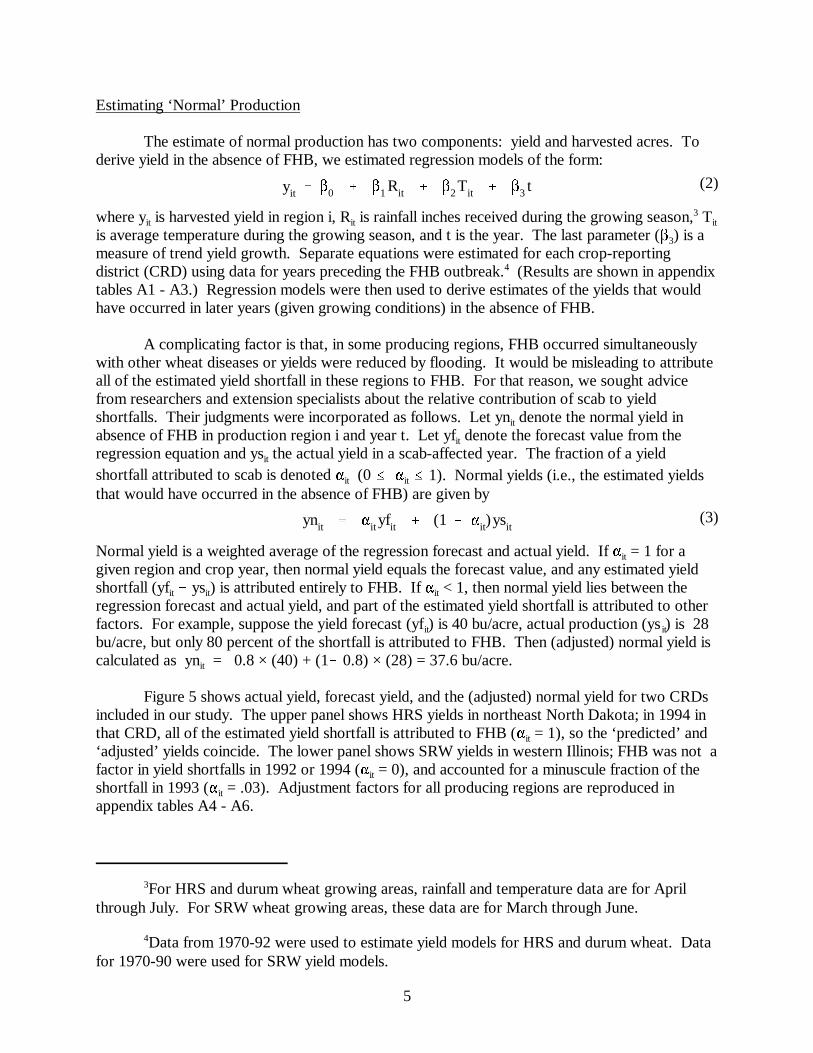
Figure 5 shows actual yield, forecast yield, and the (adjusted) normal yield for two CRDsincluded in our study. The upper panel shows HRS yields in northeast North Dakota; in 1994 inthat CRD, all of the estimated yield shortfall is attributed to FHB (� = 1), so the ‘predicted’ andit
‘adjusted’ yields coincide. The lower panel shows SRW yields in western Illinois; FHB was not afactor in yield shortfalls in 1992 or 1994 (� = 0), and accounted for a minuscule fraction of theit
shortfall in 1993 (� = .03). Adjustment factors for all producing regions are reproduced init
appendix tables A4 - A6.

HRS - ND - NE
1993 1994 1995 1996 199725
30
35
40
45
50
55
Year
Bu/Ac
Predicted Actual Adjusted
SRW - IL - W
1991 1992 1993 1994 1995 199620
30
40
50
60
70
Year
Bu/Ac
Predicted Actual Adjusted
6
Figure 5. Predicted, Actual, and Adjusted Yields in Selected CRDs

Rnit �it Ri � (1 � �it)ahit
apit
qnit [max(ynit , ysit )] # [max(Rnit ,ahit
apit
)] #apit
An olympic average omits the maximum and minimum values contained in a given5
sample. This is advantageous when the sample is small and select observations (e.g., 1988, adrought year) are viewed as exceptional or unrepresentative.
Basis is defined as the difference between a local cash price and a futures price for the6
same commodity. As used here, basis refers to the difference between weighted average cashprice received (net of premiums and discounts) and average futures during a marketing year.
7
FHB outbreaks can induce a higher-than-average rate of acreage abandonment. Toaccount for this, we incorporated a ‘normal’ ratio of harvested to planted acres in our estimate ofnormal production. This was calculated as follows. Let R represent the olympic average of thei
5
ratio (ah / ap ), where ah denotes harvested acres and ap planted acres, using data from sevenit it it it
years preceding the FHB outbreak. The ‘normal’ ratio (for region i, year t) is calculated as:
(4)
This uses the same adjustment factor as was used to calculate normal yield. If � = 1 for a givenit
region and year, then the ‘normal’ ratio of harvested to planted acres is equal to the olympicaverage. Otherwise, if � < 1, the supposition is that factors other than FHB contributed to anit
abnormal ratio, and Rn is adjusted accordingly. Normal production, denoted qn , is given by theit it
following formula:
(5)
The first bracketed term represents harvested yield. The second bracketed term is the ratio ofharvested-to-planted acres. The product of the second term and acres planted (ap ) equals normalit
harvested acres. The max function is used to correct for two types of data anomalies. If theestimated normal yield falls below actual yield in a scab year, i.e., yn < ys , the latter value isit it
selected. Similarly, if the normal ratio falls below the actual ratio of harvested-to-planted acres,i.e., Rn < (ah / ap ), the latter value is used. Thus, in the unlikely event that production is higherit it it
than normal during a scab year, the analysis will not (falsely) attribute a positive impact to thedisease.
Estimating Price Impacts
In estimating the impact of FHB on the net price received by producers, two factors mustbe considered: first, the impact of a production shortfall on market prices; and second, the qualityof the crop. To capture these effects, we divide the average price received into two components:futures and basis. While an FHB outbreak is expected to have a positive impact on futures (by6
reducing wheat supply), the impact on local basis (averaged over all wheat sold) can be eitherpositive or negative, depending on crop quality and the premiums and discounts assessed byelevators in a given region.

8
SRW wheat is generally priced with respect to wheat futures on the Chicago Board ofTrade (CBT). To derive the impact of FHB on CBT wheat futures, we first estimated aregression equation. The regression explains the CBT futures price as a function of total wheatsupply and the loan rate (a farm program parameter), using annual data from 1980 through 1996. The estimated equation follows, with t-ratios in parentheses:
LCBT = 11.250 � 1.074 LTWS + 0.601 LLR R = .652
(7.989)* (�4.984)* (3.806)* Obs. 17 * significant at 1% level
Variables are defined as:
LCBT logarithm of average CBT wheat futures price (c/bu), nearby contracts LTWS logarithm of total U.S. wheat supply (million bu), all classesLLR logarithm of loan rate for wheat (c/bu) in given marketing year
The coefficient of interest is that associated with total wheat supply (otherwise known as the‘flexibility’ coefficient). This indicates that, for a 1 percent change in total wheat supply, the CBTprice is expected to change (in the opposite direction) by 1.074 percent.
A similar equation was estimated for wheat futures on the Minneapolis Grain Exchange(MGE), which provides the standard reference for pricing of HRS wheat. In this case, we usedHRS supply (in place of total wheat supply) as an explanatory variable. For MGE futures, theestimated equation follows, with t-ratios in parentheses:
LMGE = 9.570 � 0.856 LHRS + 0.361 LLR R = .612
(6.161)* (�4.075)* (2.593)** Obs. 17
* significant at 1% level** significant at 5%
Variables are defined as:
LMGE logarithm of average MGE wheat futures price (c/bu), nearby contracts LHRS logarithm of HRS wheat supply (million bu)LLR logarithm of loan rate for wheat (c/bu) in given marketing year
The ‘flexibility’ coefficient is �0.856, indicating that for a 1 percent change in the supply of HRSwheat, the average MGE futures price is expected to change by 0.856 percent in the oppositedirection.
Adjustment for Imports
If U.S. wheat supplies were determined solely by domestic production and beginningstocks, the change in supplies due to scab would be equal to the sum of estimated productionshortfalls in affected CRDs. However, imports of wheat from Canada represent another

QnHRSt QsHRS
t � HRSt � min[�HRS
t (M HRSt � 20) , �HRS
t HRSt ]
HRS is a U.S. classification; the comparable Canadian wheat is Canadian Western Red7
Spring (CWRS).
For 1993-97, values of � are 0.6985, 0.9116, 0.5267, 0.4068, and 0.5109.8 HRSt
9
component of U.S. supply. Canada is a large surplus producer of spring wheat (HRS and7
durum), and the surge in U.S. imports since 1993 (Table 1) is partly explained by diseaseproblems in the U.S. spring wheat region. With higher imports offsetting part of a U.S.production shortfall, the change in U.S. supply is less than it otherwise would be. This reducesthe positive impact of a U.S. production shortfall on futures prices.
To account for the imports induced by scab, we begin with the assumption that 20 millionbushels of HRS wheat would be imported annually from Canada under ordinary conditions. Thatis the average level of HRS imports during the three marketing years preceding 1993. Imports ofHRS were smaller than estimated production shortfalls due to scab in four of five years; in 1996,imports exceeded the shortfall (Table 1). Of the imports exceeding 20 million bushels, only partcan be attributed to scab. That is reflected in the formula for expected HRS supply in absence ofa scab outbreak:
(6)
where variables are definedQn hypothetical supply (million bushels) of HRS wheat in absence of scabt
HRS
outbreakQs actual supply of HRS during year of scab outbreakt
HRS
estimated U.S. production shortfall of HRS wheat due to scab t HRS
� proportion of production losses due to scab, a weighted average of adjustmentt HRS
factors � in HRS regionsit8
M actual imports of HRS wheat.t HRS
Table 1. Imports From Canada and Estimated U.S. Production Losses, HRS and Durum
HRS wheat Durum wheat
Marketing Canada losses imports to Canada losses imports toyear (million bu) (million bu) losses (million bu) (million bu) losses
Imports from production Ratio of from production Ratio ofEstimated U.S. Imports Estimated U.S.
1990 10 * * 17 * *
1991 15 * * 18 * *
1992 34 * * 27 * *
1993 62 122.39 0.51 30 10.18 2.95
1994 49 92.15 0.53 22 4.01 5.49
1995 30 49.12 0.61 18 6.39 2.82
1996 53 23.66 2.24 24 8.39 2.86
1997 54 69.26 0.78 26 4.38 5.94
* Not calculated for years of insignificant FHB losses.

QnALLt QsALL
t � (QnHRSt � QsHRS
t ) � SRWt
Fn jt
Fsjt
�j
Qs jt � Qn j
t
Qn jt
� 1
The price flexibility coefficient is defined: � = (�P/P)/ (�Q/Q). The formula is derived9
by substituting (Fs � Fn)/Fn for the numerator and (Qs � Qn)/Qn for the denominator andrearranging to solve for Fn.
10
The quantity selected by the min function represents imports attributable to scab; this partiallyoffsets the impact of a production loss on U.S. supply of HRS wheat. The hypothetical supply ofall wheat in absence of scab, Qn , is calculated as:t
ALL
(7)
where Qs is the actual U.S. supply of all wheat classes and is the estimated SRW t tALL SRW
production shortfall due to scab. Note that Qn reflects the production shortfall for SRW andtALL
supply reduction for HRS; it does not reflect reduced durum production. Based on recent history(Table 1), we assume that any lost U.S. durum production would be entirely offset by importsfrom Canada.
Impacts on Futures and Basis
Given the flexibility coefficients and supply estimates, the futures prices that would havebeen observed in the absence of a scab outbreak are estimated as follows: 9
(8)
where j indicates the futures exchange (MGE or CBT) or appropriate supply category, andvariables are defined:
� price flexibility coefficient (for indicated futures supply category)j
Qs actual wheat supply (HRS wheat for MGE futures, all wheat classes for CBT)tj
Qn estimated supply in absence of scab outbreaktj
Fs futures price (annual average, nearby contracts) in a scab yeartj
Fn estimated futures price in absence of scab outbreaktj
For soft red winter (SRW) growing regions, basis is defined as the difference between theaverage price received by producers and the average CBT futures. For HRS growing regions,basis is the difference between average price received and average MGE futures. Normal basisrelationships for these wheat classes are represented by seven-year olympic averages, using datafrom years preceding the first scab outbreak.
Durum wheat was not traded on any futures exchange during the period under study. However, a long-term relationship has been observed between durum and spring wheat cash

SRW: pnSRWit Fn C
t � bn Ci
HRS: pnHRSit Fn M
t � bn Mi
Durum: pnDit Fn M
t � bn Mi � 0.50
That is approximately the price premium necessary to induce farmers to plant durum10
instead of HRS wheat, given differences in yield and risk factors.
However, state average prices were used for North Dakota CRDs in 1997, as more11
detailed information was not yet available.
11
prices: durum tends to trade at about 50 cents/bushel above the spring wheat price. This10
assumption is built into our estimate of the ‘normal’ cash price for durum.
Expected cash prices in absence of scab are calculated as follows:
(9)
where variables are defined: pn normal (expected) cash price in absence of scab for indicated wheat classit
Fn Chicago wheat futures price (annual average)tC
Fn Minneapolis spring wheat futures price (annual average)tM
bn normal (olympic average) SRW basis relative to CBT futuresiC
bn normal (olympic average) HRS basis relative to MGE futures iM
The analysis allows estimated basis effects to be either positive or negative in individual regions. Positive basis effects could arise because of large price premiums, induced by supply shortages,for wheat that meets milling specifications. Conversely, negative basis effects could result ifquality-related price discounts apply to a larger-than-average portion of local production.
Data Sources
Data on temperature and precipitation by region were obtained from the National ClimaticData Center (U.S. Department of Commerce). Data on planted and harvested acres, harvestedyield, production, and average prices received by producers were obtained from the NationalAgricultural Statistics Service (U.S. Department of Agriculture). Average CBT and MGE futuresprices were derived from a database of weekly quotes collected from Grain Market News (U.S.Department of Agriculture) and the Wall Street Journal. Basis was calculated as the differencebetween average price received in a region and the average futures price. For North Dakota,prices received were available by crop reporting district; in other states, prices are based on stateaverages. Prices for the 1997 marketing year were based on data available through February,11
1998. Data on national wheat supplies are from the Wheat Yearbook published by the EconomicResearch Service of the U.S. Department of Agriculture.

McMullen, et al. estimate a larger spring wheat (HRS and durum) production loss in12
1993: 156 million bushels in the Dakotas and Minnesota, versus 132 million bushels in this study. However, their estimate appears to have been based on comparisons with 1992, a year ofhistorically high yields in the region. Our estimates of yield loss are based on predictions fromregression models.
12
4. Results
Estimated production losses due to scab, by state and wheat class, are shown in Table 2. Aggregate losses were largest in 1993. Of the total estimated losses of 133.9 million bushelsin1993, HRS wheat accounted for 122.4 million bushels. HRS losses were also extremely large12
in 1994 and 1997. During the entire period (1991-97), HRS wheat accounted for 76 percent ofscab-related production losses, SRW wheat 17 percent, and durum 7 percent. North Dakota andMinnesota had the largest cumulative losses, followed by Illinois.
Table 2. Production Losses Due to FHB by State, Class, and Year
State/Class Year
1991 1993 1994 1995 1996 1997
------------------------------------million bu------------------------------------
HRS
N. Dakota - 63.26 39.65 27.18 16.29 38.85
Minnesota - 47.07 50.58 21.42 7.37 29.28
S. Dakota - 12.06 1.91 0.52 0.00 1.13
Total HRS - 122.39 92.15 49.12 23.66 69.26
Durum
N. Dakota - 10.02 3.82 6.28 8.36 4.38
Minnesota - 0.16 0.19 0.11 0.03 0.00
Total Durum - 10.18 4.01 6.39 8.39 4.38
SRW
Illinois 24.35 0.75 - 4.71 10.25 -
Indiana 0.00 0.00 - 0.06 1.16 -
Kentucky 0.00 0.02 - 0.02 0.01 -
Michigan 0.00 0.00 - 0.00 3.42 -
Missouri 8.67 0.26 - 2.76 3.26 -
Ohio 6.59 0.30 - 1.38 11.50 -
Total SRW 39.61 1.33 - 8.93 30.05 -
All Classes
Total 39.61 133.90 96.15 64.44 62.10 73.64

13
Table 3 shows the estimated impact of scab-related production losses on futures prices. The CBT futures price reflects national wheat supplies, while the MGE futures price reflects HRSsupplies. The estimated impact on MGE futures was generally more pronounced (except in 1996)because of differences in flexibility coefficients and larger proportionate changes in supplies ofHRS wheat. In 1993, the year of largest production losses, the MGE futures price is estimated tohave risen by 30 cents per bushel as a result of scab, while the CBT futures price is estimated tohave risen by 10 cents per bushel.
Table 3. Estimated Impact of Supply Reductions on Wheat Futures Prices
Chicago Board of Trade (CBT) Minneapolis Grain Exchange (MGE)Wheat Futures (cents/bu) Spring Wheat Futures (cents/bu)
Marketing Actual absence of Actual absence ofYear futures price scab Difference futures price scab Difference
Hypothetical Hypotheticalprice in price in
1991 354 351 3 * * *
1992 * * * * * *
1993 332 322 10 346 316 30
1994 * * * 368 345 23
1995 493 482 11 503 479 24
1996 414 406 8 430 424 6
1997 * * * 384† 363 21
† 1997 price based on average of nearby contract prices through February 1998.* Not calculated for years of insignificant FHB losses.
Estimated effects on basis are shown in Tables 4 and 5. These are calculated as thedifference between actual basis and the olympic average basis (for years preceding scab outbreak)for each producing region. The effects vary substantially through time and across regions. In1993, the basis in HRS regions was higher than the olympic average—by as much as 106 centsper bushel in north central North Dakota and by 12 cents in Minnesota. The variation acrossregions reflects differences in the (weighted) average of premiums and discounts received byproducers at local elevators. Some regions appear to have benefitted from unusually highpremiums for milling quality wheat in 1993. In other years, mixed effects are evident. Negativeeffects can arise because of steep price discounts and poor average quality. In SRW producingregions, the estimated effects on basis were strongly negative in 1991 and 1995, but positive in1996.

14
Table 4. Basis in Scab-affected HRS Regions†
NC-ND NE-ND C-ND EC-ND SE-ND SD MN
Year Actual basis in scab-affected regions (cents/bu)
1993 67 �6 62 3 11 12 �16
1994 �33 �44 �19 �23 �12 �6 �35
1995 �23 �41 �31 �33 �24 �21 �33
1996 �29 �9 �28 �2 �12 �23 �6
1997 �30 �30 �30 �30 �30 �28 �24
Olympic average basis for HRS regions prior to scab outbreak (cents/bu)
�39 �29 �21 �23 �17 �18 �28
Year Difference (actual basis minus olympic average) (cents/bu)
1993 106 23 83 26 28 30 12
1994 6 �15 2 0 5 12 �7
1995 16 �12 �10 �10 �7 �3 �5
1996 10 20 �7 21 5 �5 22
1997 9 �1 �9 �7 �13 �10 4† Basis calculated as average spring-wheat price received by producers minus average MGE futures for specified marketing year. Prices received are only available at the state level for Minnesota and South Dakota. See text for derivation of expected durum price.
Table 5. Basis in Scab-affected SRW Regions†
IL IN KY MI MO OH
Year Actual basis in scab-affected regions (cents/bu)
1991 �98 �82 �103 �70 �117 �61
1993 �51 �54 �49 �28 �65 �39
1995 �104 �97 �109 �83 �109 �97
1996 �2 �8 19 �23 �2 �20
Olympic average basis for SRW regions prior to scab outbreak (cents/bu)
�24 �31 �28 �34 �30 �23
Year Difference (actual basis minus olympic average) (cents/bu)
1991 �74 �51 �75 �36 �87 �38
1993 �27 �23 �21 6 �35 �16
1995 �80 �66 �81 �49 �79 �74
1996 22 23 47 11 28 3 † Basis calculated as average wheat price received by producers minus average CBT futures for specified marketing year.

15
Actual prices received, by class and region, are compared to the hypothetical ‘normal’prices (in absence of scab) in Tables 6-8. For HRS and durum wheat, actual prices are generallyhigher than ‘normal’ prices, as higher basis values (particularly in 1993) reinforce the positiveimpact on futures. For SRW wheat in most years (1996 is an exception), actual prices are lowerthan ‘normal’ prices, as lower basis values more than offset the futures impact.
Table 6. Prices for HRS Wheat in Scab-affected Regions
ND-NC ND-NE ND-C ND-EC ND-SE SD MN
Actual price received for HRS wheat (cents/bu)
1993 413 340 408 349 357 358 330
1994 335 324 349 345 356 362 333
1995 480 462 472 470 479 482 470
1996 402 422 403 429 419 408 425
1997 354 354 354 354 354 356 360
Estimated ‘normal’ price in absence of scab (cents/bu)
1993 277 287 295 293 299 298 288
1994 305 316 324 321 327 326 317
1995 439 450 458 455 461 460 451
1996 384 395 403 400 406 405 396
1997 324 334 342 340 346 345 335
Price difference (actual minus normal) (cents/bu)
1993 136 53 113 56 58 60 42
1994 20 8 25 24 29 36 16
1995 41 12 14 15 18 22 19
1996 18 27 0 29 13 3 29
1997 30 20 12 14 8 11 25

16
Table 7. Prices for Durum Wheat in Scab-affected Regions
ND-NC ND-NE ND-C ND-EC ND-SE MN
Actual price received for durum wheat (cents/bu)
1993 480 424 460 406 462 576
1994 470 434 436 397 518 598
1995 530 515 550 448 533 703
1996 440 397 512 406 431 574
1997 507 507 507 507 507 505
Estimated ‘normal’ price in absence of scab (cents/bu)
1993 327 337 345 343 349 338
1994 355 366 374 371 377 367
1995 489 500 508 505 511 501
1996 434 445 453 450 456 446
1997 374 384 392 390 396 385
Price difference (actual minus normal) (cents/bu)
1993 153 87 115 63 113 238
1994 115 68 62 26 141 231
1995 41 15 42 �57 22 202
1996 6 �48 59 �44 �25 128
1997 133 123 115 117 111 120

17
Table 8. Prices for SRW Wheat in Scab-affected Regions
IL IN KY MI ‡ MO OH
Actual price received for SRW wheat (cents/bu)
1991 256 272 251 284 237 293
1993 281 278 283 304 267 293
1995 389 396 384 410 384 396
1996 412 406 433 391 412 394
Estimated ‘normal’ price in absence of scab (cents/bu)
1991 327 320 323 317 321 328
1993 298 291 293 288 291 298
1995 458 452 454 448 452 459
1996 382 376 378 372 376 383
Price difference (actual minus normal) (cents/bu)
1991 �71 �48 �72 �33 �84 �35
1993 �17 �13 �10 16 �24 5
1995 �69 �56 �70 �38 �68 �63
1996 30 30 55 19 36 11
‡ Includes both SRW and white wheat.
The magnitude of price effects, especially in the HRS and durum regions, makes itimportant to qualify our estimates of economic losses due to scab. Some regions where scab waspresent experienced relatively small losses in their average yields. An example was north centralNorth Dakota in 1993. In that CRD, estimated production losses due to scab represented only6.8% of the ‘normal’ HRS production in 1993, and producers benefitted from an extremelyfavorable basis (due to premiums for protein and milling quality). In this instance, producersgained more from higher prices, on average, than they lost through reduced yields. The aggregatemeasures of economic loss include all regions where production was reduced by scab, even thosefor which positive price effects more than offset the value of lost production.
Table 9 shows estimates of lost crop value ($ million) due to FHB, by year and wheatclass. For the period under study, 1991-97, total losses were $1.3 billion. Of this amount, HRSwheat accounted for $806 million, or 61.8 percent. SRW wheat accounted for $425 million, or32.6 percent of the total, and durum wheat accounted for $73 million, or 5.6 percent of the total. While aggregate price effects for HRS and durum wheat were largely positive, those for SRWwheat were negative in all years save 1996, due to lower-than-average basis values. Negativeprice effects were especially severe for SRW wheat in 1995.

18
Table 9. Lost Crop Value Due to FHB by Year and Wheat Class1991 1993 1994 1995 1996 1997 Total
----------------------------------------------$ million---------------------------------------------
HRS
Production Effect * -389.95 -299.59 -225.60 -96.56 -239.83 -1,251.53
Price Effect * 225.51 54.77 49.16 60.04 55.22 444.70
Total * -164.44 -244.82 -176.44 -36.52 -184.61 -806.83
Durum
Production Effect * -39.52 -16.17 -32.70 -36.47 -19.46 -144.32
Price Effect * 32.06 12.45 9.39 -1.47 18.41 70.84
Total * -7.46 -3.72 -23.31 -37.94 -1.05 -73.48
SRW
Production Effect -115.61 -3.85 * -37.75 -117.58 * -274.79
Price Effect -73.40 -16.52 * -111.08 50.50 * -150.50
Total -189.01 -20.37 * -148.83 -67.08 * -425.29
All Classes
Production Effect -115.61 -433.32 -315.76 -296.05 -250.61 -259.29 -1,670.64
Price Effect -73.40 241.05 67.22 -52.53 109.07 73.63 365.04
Total -189.01 -192.27 -248.54 -348.58 -141.54 -185.66 -1,305.60* Losses due to FHB not significant.

State totals are for scab-affected CRDs only.13
19
Tables 10 and 11 show estimates of lost crop value by state. North Dakota experienced13
the largest cumulative losses during the period ($458 million, HRS and durum), followed byMinnesota ($428 million), Illinois ($202 million), Ohio ($129 million), and Missouri ($86 million).
Table 10. Lost Crop Value for Spring Wheat by State
1993 1994 1995 1996 1997 Total
---------------------------------$ million-----------------------------------
HRS
North Dakota
Production Effect -204.93 -128.69 -124.51 -66.33 -134.13 -658.59
Price Effect 155.96 24.32 28.24 38.18 27.52 274.22
Total -48.97 -104.37 -96.28 -28.15 -106.60 -384.37
Minnesota
Production Effect -145.48 -164.31 -98.63 -30.23 -101.75 -540.40
Price Effect 38.30 15.15 15.06 21.86 22.28 112.65
Total -107.18 -149.16 -83.57 -8.37 -79.47 -427.75
South Dakota
Production Effect -39.54 -6.59 -2.46 * -3.96 -52.55
Price Effect 31.25 15.30 5.86 * 5.41 57.82
Total -8.29 8.71 3.40 * 1.45 5.27
Durum
North Dakota
Production Effect -38.79 -15.27 -32.04 -36.31 -19.46 -141.87
Price Effect 31.30 11.60 8.55 -1.78 18.41 68.08
Total -7.49 -3.67 -23.49 -38.08 -1.05 -73.78
Minnesota
Production Effect -0.73 -0.90 -0.66 -0.17 * -2.46
Price Effect 0.76 0.85 0.84 0.31 * 2.76
Total 0.03 -0.05 0.18 0.14 * 0.30 * Losses due to FHB not significant.

20
Table 11. Lost Crop Value for SRW Wheat by State
1991 1993 1995 1996 Total
---------------------------$ million----------------------------
Illinois
Production Effect -70.99 -2.18 -19.97 -40.72 -1,33.87
Price Effect -33.10 -8.82 -36.85 10.71 -68.07
Total -104.09 -11.00 -56.83 -30.01 -201.93
Indiana
Production Effect * * -0.27 -6.29 -6.56
Price Effect * * -6.19 6.02 -0.18
Total * * -6.47 -0.27 -6.73
Kentucky
Production Effect * -0.06 -0.07 -0.04 -0.17
Price Effect * -0.57 -4.65 12.46 7.24
Total * -0.63 -4.73 12.43 7.07
Michigan
Production Effect * * * -13.04 -13.04
Price Effect * * * 4.59 4.59
Total * * * -8.44 -8.44
Missouri
Production Effect -24.18 -0.72 -11.55 -12.86 -49.30
Price Effect -22.50 -4.66 -20.72 10.75 -37.13
Total -46.68 -5.38 -32.27 -2.10 -86.44
Ohio
Production Effect -20.44 -0.89 -5.88 -44.65 -71.86
Price Effect -17.80 -2.47 -42.65 5.96 -56.97
Total -38.25 -3.36 -48.54 -38.69 -128.83 * Losses due to FHB not significant.

21
5. Summary and Discussion
During the 1990s, wheat producers in FHB-affected regions have suffered cumulativelosses of $1.3 billion, according to our analysis. This represents the estimated change in cropvalue after accounting for reduced yields, higher abandoned acres, and price impacts on futuresand basis. The economic losses have been most severe in the spring-wheat growing regions,particularly North Dakota and Minnesota. These two states account for 67.9 percent of theestimated total losses.
One of the main difficulties in measuring economic losses due to FHB is estimating theprice effects. While supply reductions tend to increase the futures price, the effects on averagebasis (difference between local cash price and futures) are less certain. Shortages of milling-quality wheat can induce large price premiums, which favor producers who have high qualitywheat to sell. However, many producers in scab-affected regions face quality discounts due todamaged kernels, low test weight, or vomitoxin. The average basis in a region depends on thequality of wheat sold by all producers and the premiums and discounts applied by local elevators. To measure the impact of scab on basis, we used deviations from olympic-average basisvalues in years preceding the scab outbreak. Results indicate that the effects on basis wereprimarily negative in the SRW regions (except in 1996), more than offsetting gains in futuresprices. In spring wheat regions, the impacts on basis varied by CRD and year. However, largepositive basis effects were estimated in 1993, the year of largest production shortfalls. Combinedwith the impact on MGE spring wheat futures, this helped to offset much of the economic lossdue to scab in that year.
The positive price effect for spring wheat that we estimated for 1993 draws attention towhat may be termed an ‘aggregation problem.’ Our analysis used CRD-level production data andCRD or state-level price data to derive the economic losses suffered by producers. Data at thislevel of aggregation do not convey the severity of losses for individual producers whose yieldsand price were lower than average. Moreover, in some CRDs where producers benefitted (onaverage) from higher prices, scab-related production losses were fairly small or localized. Ourestimates of economic loss are affected, unavoidably, by the inclusion of positive price effects forall wheat sold in a CRD—even wheat sold by producers who suffered no yield losses.
This problem notwithstanding, it is clear that many CRDs have suffered major economiclosses as a result of FHB. These losses are bound to have broader repercussions at state andregional levels, as producers’ losses are felt throughout the economy. Based on results from astate-level input-output analysis for North Dakota (Dean Bangsund and Larry Leistritz, personalcommunication), the ‘multiplier effect’ of lost crop value is substantial: for each dollar of lost cropvalue, state-level economic activity declines by $3.68, after accounting for sectoral linkages andspending patterns within the state economy. If the same multiplier held for other statesconsidered in this study, the cumulative economic impact of FHB during 1991-97 would be $4.8billion.
There is other, more tangible evidence of economic distress in scab-affected regions. Netfarm income for 1997 in the north central region of North Dakota was the lowest since 1989,down 34 percent on average from 1996, according to North Dakota Farm Business Management

22
(FBM) records (North Dakota Farm Business Management Record Program). Net farm incomeaveraged $22,528 during 1997, far short of the $35,000 that FBM records indicate is the typicalamount spent per farm for family living (including taxes) in the region. The 20 percent least-profitable farms averaged a negative $16,620 net farm income.
Income losses have resulted in a reduction in farm numbers. About 2,000 farms were lostin North Dakota during 1992-1996, versus 500 during the previous four years, according toNorth Dakota Agricultural Statistics. This trend may be accelerating during 1998. Auction salelistings (for Mid-March through May) were up 55 percent over a year ago in the March 16 issueof AGWEEK, an agricultural publication serving the northern Red River Valley (Johnson).
Loan activity by the Farm Service Agency (FSA) in northwest Minnesota has doubledsince 1997 (Carr). FSA loans are made to farms that do not qualify for regular bank operatingloans. This region, one of the hardest hit by FHB, represented 48 percent of FSA loan activity forMinnesota as of mid-March.
Revenue shortfalls are occurring at a time of rising production costs. Operating costsbetween 1991 and 1996 increased by 60 percent, according to FBM records for North Dakota. Meanwhile, government assistance is declining. Disaster payments are no longer available to theextent that they were during the early years of the disease infestation, and multi-peril cropinsurance programs provide less of a safety net since they are based on average yields, which havefallen in the last several years. These factors accentuate the problem facing producers who havesuffered repeated losses due to scab.

23
References
Bangsund, Dean A. Personal communication, May 1998.
Carr, Eugene G., ed. “Polk Farm Crises Sparks Increase in FSA Loans.” The Thirteen Towns. March 30, 1998.
Johnson, Rona K., ed. “Upcoming Auctions.” AGWEEK, March 17, 1997 and March 16, 1998.
Leistritz, F. Larry. Personal communication, October, 1997.
McMullen, Marcia, Roger Jones, and Dale Gallenberg. 1997. “Scab of Wheat and Barley: A Re-emerging Disease of Devastating Impact.” Plant Disease, Vol. 81: 1340-1348.
National Climatic Data Center, Office of Environmental Information Service, National Oceanicand Atmospheric Administration, U.S. Department of Commerce.
North Dakota Agricultural Statistics. June, 1997. “Number of Farms and Land in Farms byEconomic Class, North Dakota, 1987-96.”
North Dakota Farm Business Management Record Program. Annual Reports, 1991-97, NorthDakota Vocational - Technical Education.
U.S. Department of Agriculture, Agricultural Marketing Service, Grain and Feed Division. GrainMarket News, various issues.
U.S. Department of Agriculture, National Agricultural Statistics Service. Data diskette.
U.S. Department of Agriculture, Economic Research Service. Wheat Yearbook. Various years.
Wall Street Journal, various issues.

24
Appendix Tables
Table A1. HRS Wheat Yield Equation Parameter Estimates, by StateState / CRD Intercept Trend Temperature Precipitation R2 Adj. R2 Sample
Size
ND - NC 94.227 0.32133 -1.4173 0.64874 0.4029 0.2976 21
( 3.305) ( 1.685) (-2.890) ( 1.297)
ND - NE 85.402 0.5673 -1.0613 0.47697 0.3101 0.1883 21
( 2.285) ( 2.337) (-1.698) (0.7834)
ND - C 75.725 0.33886 -1.0997 1.0742 0.4323 0.3321 21
( 2.423) ( 1.669) (-2.103) ( 2.110)
ND - EC 93.574 0.63324 -1.2613 0.60845 0.3619 0.2493 21
( 2.415) ( 2.590) (-1.922) ( 1.138)
ND - SE 78.095 0.40425 -1.0025 0.26589 0.2333 0.098 21
( 1.935) ( 1.803) (-1.511) (0.5233)
MN - NW 70.111 0.72676 -0.88439 1.0175 0.4083 0.3039 21
( 1.522) ( 2.842) (-1.157) ( 1.528)
MN - WC ** 46.37 0.61307 -0.54676 1.2211 0.3581 0.2448 21
( 0.9857) ( 2.788) (-0.7331) ( 2.189)
MN - C ** -26.752 0.20103 0.91152 0.46975 0.1508 0.001 21
(-0.4797) ( 0.6544) ( 1.017) ( 0.9343)
SD - NC 79.998 0.36576 -1.134 0.58488 0.3396 0.223 21
( 1.714) ( 1.710) (-1.571) (0.8920)
SD - NE ** 36.78 0.47997 -0.47984 1.2704 0.3232 0.2037 21
( 0.8842) ( 2.576) (-0.7205) ( 2.563)
SD - C 84.557 0.32151 -1.1035 -0.047464 0.291 0.1659 21
-1.702 -1.289 ( -1.452 ) (-0.079)
Numbers in the parentheses are t-values
** Indicates error structure corrected for first order autocorrelation

25
Table A2. Durum Wheat Yield Equation Parameter Estimates, by StateState / CRD Intercept Trend Temperature Precipitation R2 Adj. R2 Sample Size
ND - NC 98.817 0.32251 -1.4729 0.70589 0.4058 0.3009 21
( 3.332) ( 1.625) (-2.887) ( 1.356)
ND - NE 84.35 0.36631 -1.1761 0.82275 0.3616 0.2489 21
( 2.798) ( 1.829) (-2.275) ( 1.475)
ND - C 82.668 0.46442 -1.2943 1.3865 0.5387 0.4573 21
( 2.616) ( 2.263) (-2.449) ( 2.693)
ND - EC 94.682 0.85496 -1.3889 0.87211 0.4673 0.3733 21
( 2.348) ( 3.360) (-2.033) ( 1.567)
ND - SE 65.407 0.5025 -0.89617 0.83324 0.3908 0.2832 21
( 1.750) ( 2.420) (-1.459) ( 1.771)
MN - NW 61.129 0.6421 -0.82059 1.4907 0.4763 0.3838 21
( 1.416) ( 2.678) (-1.145) ( 2.387)
MN - WC ** 35.806 0.42769 -0.39002 1.2589 0.4217 0.3197 21
( 1.044) ( 2.674) (-0.7170) ( 3.084)
Numbers in the parentheses are t-values
** Indicates error structures corrected for first order autoregression

26
Table A3. SRW Yield Equation Parameter Estimates, by StateState / CRD Intercept Trend Temperature Precipitation R2 Adj. Sample Size
R2
IL - W 56.233 1.2241 -0.24502 -0.58471 0.6816 0.6179 19
-1.279 -4.483 (-0.3298) ( -1.742)
IL - WSW 75.505 0.93293 -0.4845 -0.61913 0.6284 0.5541 19
-1.783 -3.799 (-0.6918) ( -1.884)
IL - ESE 35.662 0.85432 0.21217 -0.73802 0.6479 0.5775 19
-0.8517 -3.77 -0.3069 (-2.286)
IL - SW 80.715 0.80986 -0.55467 -0.83165 0.6176 0.5412 19
-1.86 -3.643 (-0.7916) ( -2.814)
IL - SE -2.2713 0.79954 0.7623 -0.62178 0.5553 0.4664 19
(-0.04404) -3.272 -0.9269 ( -1.910)
IN - NE ** 70.906 0.89601 -0.57457 -0.17975 0.6339 0.5606 19
-2.351 -6.03 ( -1.111) (-0.4213)
IN - C ** 90.46 1.0548 -0.7959 -0.36563 0.7873 0.7447 19
-3.339 -9.376 (-1.763) (-1.292)
IN - SW 29.112 0.76875 0.22551 -0.39652 0.4521 0.3426 19
-0.5295 -3.081 -0.2547 (-1.101)
IN - SC ** 42.918 0.66552 -0.16107 -0.073021 0.4488 0.3386 19
-1.015 -3.651 (-0.2327) (-0.2520)
IN - SE 33.704 0.90967 0.013917 -0.25987 0.6554 0.5864 19
-0.7634 -4.818 -0.01932 (-0.8592)
KY - PUR ** 4.975 0.74822 0.46648 -0.27356 0.5624 0.4749 19
-0.0909 -2.577 -0.5423 (-1.060)
KY - MW 63.983 0.6774 -0.40115 -0.37702 0.4075 0.2889 19
-0.8769 -2.169 (-0.3477) (-0.8993)
MI - C 46.362 0.7124 -0.33776 0.51998 0.3094 0.1713 19
-1.105 -2.529 (-0.4099) -0.9605
MI - EC 33.645 1.3381 -0.087447 0.79063 0.6995 0.6394 19
-0.9666 -5.78 (-0.1301) -1.771
MI - SW 57.557 0.88435 -0.52123 0.093666 0.4865 0.3838 19
-1.543 -3.208 (-0.7884) -0.1458
MI - SC 76.68 0.88382 -0.8258 0.013682 0.4688 0.3626 19
-1.805 -3.181 (-1.081) -0.02038
MI - SE 54.808 0.99427 -0.46167 0.36915 0.6047 0.5257 19
-1.64 -4.657 (-0.7414) -0.6588
MO - NE ** 76.348 0.74045 -0.58409 -0.51745 0.3678 0.2414 19
-1.543 -2.953 (-0.7318) ( -1.294)

Table A3 (Cont.)
State / CRD Intercept Trend Temperature Precipitation R2 Adj. Sample SizeR2
27
MO - E 42.048 0.54152 -0.005345 -0.47311 0.4246 0.3095 19
-0.9438 -2.516 (-0.007128) ( -1.783)
MO - SW 95.491 0.48229 -0.96776 -0.43828 0.4027 0.2832 19
-2.16 -2.27 (-1.333) (-1.645)
MO - SC 38.84 0.58563 -0.10129 -0.38543 0.4907 0.3888 19
-1.002 -3.128 (-0.1553) ( -1.670)
MO - SE ** 53.13 0.18257 0.0076974 -0.89689 0.3791 0.255 19
-1.803 -0.8101 -0.01441 (-2.865)
OH - NW ** 11.227 0.88812 0.42239 0.55772 0.5406 0.4487 19
-0.258 -4.883 -0.5589 -0.899
OH - NC ** 14.405 0.95953 0.41396 0.0062829 0.6824 0.6188 19
-0.4492 -6.564 -0.7199 -0.01602
OH - NE ** 0.68114 0.88102 0.60395 -0.077001 0.7398 0.6877 19
-0.0267 -8.242 -1.282 (-0.2230 )
OH - WC ** 30.901 0.92016 0.24147 -0.29203 0.6805 0.6166 19
-0.9204 -6.548 -0.4161 (-0.9234)
OH - C ** 17.405 1.0137 0.4663 -0.5433 0.8358 0.803 19
-0.6465 -11.11 -1.031 (-2.278)
Numbers in the parentheses are t-values
**Indicates error structures corrected for first order autoregression

28
Table A4. Fraction of SRW Yield and Area Loss Attributable to FHB (� ), by State and Yearit
Year IL IN KY MI MO OH
1991 0.7 0 0 0 0.7 0.7
1992 0.01 0 0.02 0 0.01 0.01
1993 0.05 0 0.05 0 0.05 0.05
1994 0.05 0 0.01 0 0.05 0.05
1995 0.65 0.1 0.05 0 0.65 0.65
1996 0.45 0.16 0.01 0.2 0.45 0.45
Source: Extension Specialists
Note: fractions for Missouri and Ohio were assumed to be identical to those for Illinois
Table A5. Fraction of HRS Yield and Area Loss Attributable to FHB (� ), by CRD and Yearit
Year NC NE ND-C EC SE NW WC MN-C NC NE SD-CND- ND- ND- ND- MN- MN- SD- SD-
1993 0.5 0.6 0.6 0.6 1 0.8 0.7 0.7 0.7 0.7 0.7
1994 0 1 1 0.8 0 0.9 1 1 0.2 0.5 0.2
1995 0.2 0.6 0.25 0.2 0.1 0.6 0.1 0.1 0.1 0.1 0.1
1996 0.33 0.5 0.33 0.25 0 0.35 0 0 0 0 0
1997 0.5 0.4 0.25 0.6 0.2 0.6 0.2 0.2 0.2 0.2 0.2
Source: Extension specialists.
Table A6. Fraction of Durum Yield and Area Loss Attributable to FHB (� ), by CRD and Yearit
Year ND-NC ND-NE ND-C ND-EC ND-SE NW WCMN- MN-
1993 0.35 0.7 0.7 0.7 1 0.7 0.7
1994 0 0.6 0.5 0.7 1 0.6 0.7
1995 0.3 0.5 0.5 0.7 0.8 0.5 0.7
1996 0.7 0.6 0.7 0.7 0.8 0.6 0
1997 0.4 0.55 0.7 0.7 0.8 0 0
Source: Extension specialists.