ECONOMIC IMPACT OF AGRICULTURAL BIOTECHNOLOGY IN …

Katholieke Universiteit Leuven Faculteit Bio-ingenieurswetenschappen

DISSERTATIONES DE AGRICULTURA

Doctoraatsproefschrift nr. 713 aan de faculteit Bio-ingenieurswetenschappen van de K.U.Leuven

ECONOMIC IMPACT OF AGRICULTURAL BIOTECHNOLOGY IN THE EUROPEAN UNION:

TRANSGENIC SUGAR BEET AND MAIZE

Proefschrift voorgedragen tot het behalen van de graad van Doctor in de Bio-ingenieurswetenschappen door Matty DEMONT

SEPTEMBER 2006


Katholieke Universiteit Leuven Faculteit Bio-ingenieurswetenschappen

DISSERTATIONES DE AGRICULTURA


ECONOMIC IMPACT OF AGRICULTURAL BIOTECHNOLOGY IN THE EUROPEAN UNION:

TRANSGENIC SUGAR BEET AND MAIZE Promotor: Proefschrift voorgedragen tot het Prof. E. Tollens, K.U.Leuven behalen van de graad van

Doctor in de Bio-ingenieurswetenschappen

Leden van de examencommissie: Prof. G. Volckaert, K.U.Leuven, voorzitter door Prof. E. Mathijs, K.U.Leuven Matty DEMONT Prof. J. Vanderleyden, K.U.Leuven Prof. J. Swinnen, K.U.Leuven Prof. J. Wesseler, Wageningen Universiteit

SEPTEMBER 2006

i

Preface

I would like to dedicate this doctoral dissertation to my mother, Lutgart Wauman, who unexpectedly passed away on the 21st of January 2006. She is present in every formula of this study, because precision is one of the greatest things I learned from her. I am proud to hand over this work into the living hands of my father and would like to thank my parents for all the great opportunities I received as eternal student. The EUWAB project (1999-2006) In May 1999, the EUWAB project (European Union Welfare effects of Agricultural Biotechnology) has been founded at the Centre of Agricultural and Food Economics of the Katholieke Universiteit Leuven. The main objective of this project is to support the debate on agricultural biotechnology in Flanders, Belgium and the European Union (EU). More specifically, the project aims at generating economic impact data of transgenic crops in the EU to support the debate on the economic aspects of biotechnology. Therefore, it aims at assessing the potential welfare effects of agricultural biotechnology innovations in the European Union and their distribution among Member States and stakeholders in the food chain. From May 1999 to October 2002, the project has been financed by the Flanders Interuniversity Institute for Biotechnology (VIB), and since November 2002 by the K.U.Leuven, the European Commission’s 6th Framework Programme and Monsanto. During this period, the EUWAB project has been valorised through the following output:

• 3 international peer reviewed journal publications;

• 4 international peer reviewed book chapters;

• 15 international peer reviewed conference papers and presentations;

• 20 national seminar papers, presentations and courses;

• EUWAB website: http://www.biw.kuleuven.be/aee/clo/euwab.htm;

• 5 national extension publications;

• 18 working paper publications;

• Collection of more than 2,200 scientific articles on the impact of agricultural biotechnology and technological change. The full reference list is accessible from the website.

The EUWAB project is well established in international research and policy scenes. Its extensive valorisation led to the following international spillovers:

• 41 international publications refer to the EUWAB project;

• 80 international press releases are related to the EUWAB project;

• 21 international websites refer to the EUWAB project.

ii

Acknowledgements First of all, I would like to thank my promoter, Prof. Eric Tollens, for giving me the opportunity and the freedom to work on such an interesting and controversial topic. Secondly, the EUWAB project would not have existed without the valuable financial support from the Flanders Interuniversity Institute for Biotechnology (VIB), the Katholieke Universiteit Leuven, the European Commission’s 6th Framework Programme and Monsanto.

I would like to express my gratitude to the following persons for providing feedback on several parts of this dissertation: Julian M. Alston (UC Davis), José Falck-Zepeda (IFPRI, Washington), Brent Borrell (The CIE, Canberra), Ivan Roberts (ABARE, Canberra), James F. Oehmke (Michigan State University, East Lansing), Richard Gray (University of Saskatchewan), Justus Wesseler (Wageningen University), Sara Scatasta (ZEW, Mannheim), René Lahousse (Bayer CropScience), René Custers (VIB, Ghent), József Kiss (Szent Istvan University, Gödöllõ), József Fogarasi (AKI, Budapest), François Huyghe (Boerenbond, Leuven), Jozef Claes (Boerenbond, Leuven), Harvey Glick (Monsanto, St. Louis), Thierry Merckling (Monsanto, France), Francesca Tencalla (Monsanto, Brussels), Jean-François Misonne (IRBAB, Tienen), Olivier Hermann (IRBAB, Tienen) and Johan De Rycker (Raffinaderij Tienen).

I also would like to thank the following persons for their valuable advice on several topics covered in this dissertation: Giancarlo Moschini (Iowa State University), Andrei Sobolevsky (Sprint, Kansas), Robert E. Evenson (Yale University), William Lin (USDA, Washington), Peter D. Goldsmith (University of Illinois, Urbana-Champaign), Nicholas Kalaitzandonakas (University of Missouri), Marc Van Montagu (Ghent University), Matin Qaim (University of Hohenheim, Stuttgart), Christos J. Pantzios (University of Patras), Stéphane Lemarié (INRA, Grenoble), Michele Marra (North Carolina State University), Terrance Hurley (University of Minnesota), Paul D. Mitchell (Texas A&M University), Graham Brookes (PG Economics, Dorset), Murray Fulton (University of Saskatchewan), Alex Krick (CIBE, France), Thierry Gestat De Garambé (ITB, Paris), Stanislav Tobola (Moravskoslezské cukrovary, Hrušovany nad Jevišovkou, Czech Republic), Wim Daems (Katholieke Universiteit Leuven), Daniel Du Ville (CBB, Brussels), Jean-François Sneessens (CBB, Brussels) and the editors and reviewers of European Review of Agricultural Economics, Annals of Applied Biology, Outlook on Agriculture, Agricultural Systems, CAB International, and Springer. Finally, I am grateful to the Members of the Jury for reviewing this manuscript and providing valuable suggestions: Prof. Guido Volckaert, Prof. Jos Vanderleyden, Prof. Johan Swinnen and Prof. Erik Mathijs from the Katholieke Universiteit Leuven, and Prof. Justus Wesseler from Wageningen University.

iii

Publication list International peer reviewed journal articles Demont, M., J. Wesseler, and E. Tollens. “Biodiversity versus transgenic sugar beets:

The one Euro question.” European Review of Agricultural Economics 31(2004):1-18. (2005 Impact factor: 0.977)

Demont, M., and E. Tollens. “First impact of biotechnology in the EU: Bt maize adoption in Spain.” Annals of Applied Biology 145(2004):197-207. (2005 Impact factor: 1.060)

Tollens, E., M. Demont, and R. Swennen. “Agrobiotechnology in developing countries: North-South partnerships are a key.” Outlook on Agriculture 33(2004):231-38. (2005 Impact factor: 0.421)

Demont, M., Jouve, P., Stessens, J., and E. Tollens. “Boserup versus Malthus revisited: evolution of farming systems in Northern Côte d’Ivoire.” Forthcoming in Agricultural Systems. (2005 Impact factor: 0.937)

International peer reviewed book chapters Demont, M., and E. Tollens. “Ex ante welfare effects of agricultural biotechnology in

the European Union: The case of transgenic herbicide tolerant sugarbeet.” The regulation of agricultural biotechnology. Evenson, R.E., and V. Santaniello, ed., pp. 239-255. Wallingford, UK: CAB International, 2004.

Demont, M., J. Wesseler, and E. Tollens. “Irreversible costs and benefits of transgenic crops: what are they?” Environmental costs and benefits of transgenic crops. Wesseler, J., ed., pp. 113-122. Dordrecht, NL: Springer, 2005.

Scatasta, S., J. Wesseler, and M. Demont. “Irreversibility, uncertainty, and the adoption of transgenic crops: experiences from applications to HT sugar beet, HT corn, and Bt Corn.” Regulating agricultural biotechnology: Economics and policy. Alston, J.M., R.E. Just, and D. Zilberman, ed., pp. 1-26. Berlin, DE: Springer, 2006.

International non-peer reviewed publications

Scatasta, S., J. Wesseler, and M. Demont. “A critical assessment of methods for analysis of social welfare impacts of genetically modified crops: A literature survey.” Discussion Paper, n° 27, Mansholt Graduate School, Wageningen, 2006.

iv

Table of contents Preface.......................................................................................................................i Publication list.........................................................................................................iii Table of contents .....................................................................................................iv Samenvatting..........................................................................................................vii Abstract ................................................................................................................... ix Abbreviations..........................................................................................................xi Introduction .............................................................................................................1

The study of innovation in agriculture....................................................................1 The basic model .................................................................................................1 Privately funded R&D protected by intellectual property rights .........................3

Biotechnology innovations in agriculture ...............................................................4 Distributional issues...........................................................................................5 Regulatory issues ...............................................................................................8 Externalities .......................................................................................................9

Objective .............................................................................................................10 Hypotheses.......................................................................................................10 Selection of case studies ...................................................................................11 Delimitation of the study ..................................................................................14

Chapter 1: Ex ante welfare effects of agricultural biotechnology in the EU-15: The case of transgenic herbicide tolerant sugar beet............................................17

Introduction .........................................................................................................17 Sugar ...................................................................................................................17 Transgenic sugar beets .........................................................................................19 The model............................................................................................................19 Data and model calibration...................................................................................30 Results .................................................................................................................35 Conclusion...........................................................................................................40

Chapter 2: Biodiversity versus transgenic sugar beet: The one Euro question...41 Introduction .........................................................................................................41 Reversible and irreversible private and social benefits and costs...........................41 Theoretical model ................................................................................................43

Defining the maximum tolerable irreversible costs ...........................................43 Defining the social reversible net benefits W ....................................................46 Defining the social irreversible benefits R ........................................................48

Data .....................................................................................................................48 Results and discussion..........................................................................................51 Conclusion...........................................................................................................53

v

Chapter 3: First impact of biotechnology in the EU: Bt maize adoption in Spain................................................................................................................................ 55

Introduction......................................................................................................... 55 Economic importance of maize on a world-wide scale ......................................... 55 Economic importance of maize crop protection ................................................... 56

The corn borer................................................................................................. 56 Crop protection: insecticides, Bt and Bt maize................................................. 57 Adoption of Bt maize........................................................................................ 58

Model.................................................................................................................. 59 Data..................................................................................................................... 61

Insecticide use and cost ................................................................................... 61 Technology fee................................................................................................. 62 Theoretical loss due to corn borers.................................................................. 62 Efficacy of both technologies ........................................................................... 63 All other costs.................................................................................................. 64 Other parameters............................................................................................. 65

Results................................................................................................................. 65 Average impact results..................................................................................... 65 Uncertainty...................................................................................................... 65 Sensitivity analysis........................................................................................... 67 Discussion ....................................................................................................... 68

Conclusion .......................................................................................................... 69 Chapter 4: Alston, Norton, and Pardey revisited: Modelling supply shift in equilibrium displacement models ......................................................................... 71

Introduction......................................................................................................... 71 Modelling welfare effects .................................................................................... 73

Change in revenue method (CIR)..................................................................... 74 Alston, Norton, and Pardey (1995) .................................................................. 74 Moschini, Lapan, and Sobolevsky (2000) (MLS) .............................................. 75 Comparative static results ............................................................................... 76

Data..................................................................................................................... 77 Results................................................................................................................. 78

Central tendencies and dispersion ................................................................... 78 Robustness of the models and sensitivity to individual parameters ................... 82 Discussion ....................................................................................................... 85

Conclusion .......................................................................................................... 87 Chapter 5: Pathways for future research ............................................................. 89

The reform of the European sugar regime ............................................................ 89 Traceability and labelling .................................................................................... 91

vi

Coexistence of GE and non-GE crops ..................................................................92 Modelling non-pecuniary benefits ........................................................................95 EU decision-making under the precautionary principle.........................................98

Chapter 6: General conclusions and recommendations..................................... 101 Hypothesis 1: The first generation of agricultural biotechnology innovations could and can significantly contribute to productivity and welfare in EU agriculture ... 101

Beet growers .................................................................................................. 101 Cane growers................................................................................................. 102 Maize farmers ................................................................................................ 103 Sugar beet processors and sugar manufacturers............................................. 103 Consumers ..................................................................................................... 103

Hypothesis 2: The largest share of total welfare creation by these innovations is captured downstream ......................................................................................... 104 Hypothesis 3: Conventional benefit-cost analysis can be extended by a real option approach to assess maximum tolerable levels of irreversible environmental costs that justify a release of these innovations in the EU............................................ 106 Hypothesis 4: Some of the variability of welfare estimates reported in literature can be explained by the modelling of supply shift in conventional equilibrium displacement models .......................................................................................... 106 Limitations of our modelling approach............................................................... 107 Recommendations for researchers ...................................................................... 111

Definition of the counterfactual...................................................................... 111 Stochastic data mining ................................................................................... 112

Recommendation for policy makers ................................................................... 113 Appendix A: Calculation of innovation rents in the land market ...................... 115

Innovation rents under normal pricing................................................................ 115 Innovation rents under mixed pricing ................................................................. 117 Supply elasticity estimates from literature .......................................................... 118

Appendix B: Structure of EUWABSIM.............................................................. 121 Software interaction ........................................................................................... 121 Solution for software interaction problem........................................................... 122 Mathematical module in EUWABSIM............................................................... 122

References ............................................................................................................ 127

vii

Samenvatting Het doel van dit doctoraatsproefschrift is een bijdrage te leveren aan de literatuur rond de impact van transgene gewassen en de rendabiliteit van landbouwkundig onderzoek en het beleidsdebat rond transgene gewassen in de Europese Unie (EU) te ondersteunen en te informeren.

In het eerste hoofdstuk ontwikkelen we een stochastisch partieel evenwichtsmodel om de grootte en de verdeling van de baten van transgene herbicidenresistente (HT) suikerbieten te schatten in de EU-15 en de rest van de wereld (RVW). Het model is dynamisch en simuleert het gedrag van de wereldprijs op huidige en historische Europese suikerexporten. De totale welvaartstoename voor de wereldeconomie wordt geschat op €1.1 miljard na vijf jaar. Het model berekent dat de RVW het grootste aandeel van deze baten absorbeert (50%), gevolgd door de Europese suikerindustrie (26%) en de zaadsector (24%). Daar interventieprijzen op Europees niveau vastgelegd worden, is er geen welvaartstoename voor Europese consumenten. Door dalende wereldprijzen winnen consumenten en verliezen suikerriettelers in de RVW. Via overdracht van technologie gaat een deel van de welvaart naar suikerbietentelers in de RVW. Opvallend is dat buitenlandse consumenten winnen, terwijl binnenlandse burgers hoge suikerprijzen blijven betalen. De nieuwe Europese marktordening voor suiker zal resulteren in lichtelijk lagere baten voor innovatie, echter zonder onze resultaten kwalitatief te veranderen.

In het tweede hoofdstuk stellen we ons in de plaats van een Europese beslissingsmaker die de beslissing moet nemen om al dan niet HT suikerbieten toe te laten in het jaar 1995. Deze beslissing is onderhevig aan flexibiliteit, onzekerheid en onomkeerbaarheid. Terwijl de meeste literatuur rond de economische impact van transgene gewassen gericht is op het schatten van directe omkeerbare baten en kosten, zoals in het eerste hoofdstuk, proberen we in het tweede hoofdstuk sociale onomkeerbare baten en kosten samen te brengen in een evaluatie van het Europees de facto moratorium op transgene gewassen. We beschouwen de EU-15 in 1995 en gaan na of de goedkeuring van HT suikerbieten in de EU al dan niet uitgesteld zou moeten worden. Volgens de neoklassieke beslissingstheorie zouden HT suikerbieten toegelaten mogen worden als de verwachte sociale omkeerbare baten minstens even groot zijn als de sociale onomkeerbare kosten. In dit geval betekent dit dat de toelatingsdrempel gelijk aan één is. Het uitdrukkelijk in rekening brengen van onzekerheid en de mogelijkheid om een beslissing uit te stellen, leidt tot een veel grotere toelatingsdrempel dan in de standaard neoklassieke theorie. De ‘real option’ theorie laat ons toe deze drempel te schatten. De nieuwe beslissingsregel bestaat er in HT suikerbieten toe te laten als de omkeerbare baten groter zijn dan de onomkeerbare kosten, vermenigvuldigd met een factor groter dan één. Daar er veel onzekerheid is

viii

over de onomkeerbare milieukosten, trachten we ze niet direct te kwantificeren, maar schatten we de ‘break-even’ kosten, namelijk de maximaal toelaatbare sociale onomkeerbare kosten. Voor afzonderlijke lidstaten variëren de break-even kosten tussen €46 en €158 per hectare, zijnde 27 tot 81% van de jaarlijkse sociale omkeerbare baten. Regio’s met een comparatief voordeel in de productie van suikerbieten (Centraal-Europa) hebben lage toelatingsdrempels en leggen zwakkere beperkingen op de break-even kosten dan regio’s zonder comparatief voordeel (Zuid- en Noord-Europa). Voor de EU-15 zijn de maximaal toelaatbare sociale onomkeerbare kosten €94 per hectare transgene suikerbieten, goed voor €77 miljoen per jaar. Deze zijn ongeveer 60 keer groter dan de sociale onomkeerbare baten. Daar beide indicatoren gelijkaardige milieueffecten bevatten, zoals impact op milieu, biodiversiteit en klimaat, is het onwaarschijnlijk dat de echte ongekende sociale onomkeerbare kosten zo hoog zouden oplopen.

In het derde hoofdstuk ontwikkelen we een model om de impact van Bt maïs in de Europese landbouw te schatten. Spanje levert 11% van de maïs in de EU-15. Twee types van maïsboorders veroorzaken ernstige schade in deze sector. Dit opent perspectieven voor transgene Bt maïs, die een efficiëntere bestrijding van deze insecten toelaat. We modelleren onzekerheid via stochastische simulaties. Gedurende de periode 1998-2003 schatten we een totale welvaartstoename van €16 miljoen dankzij de adoptie van Bt maïs, waarvan Spaanse landbouwers twee derden (67%) absorberen en de zaadindustrie één derde (33%).

Rendabiliteitschattingen van landbouwkundig onderzoek hangen sterk af van de geschatte aanbodsverschuiving. In het vierde hoofdstuk vergelijken we algebraïsch vijf verschillende manieren om deze verschuiving te modelleren, vaak gebruikt in de literatuur rond de impact van transgene gewassen. We rekenen de modellen na met de stochastische resultaten uit het derde hoofdstuk. Via Monte Carlo simulaties worden distributies gegenereerd voor het producentensurplus en de aanbodsrespons die geschat wordt door de modellen. Via een variantieanalyse worden het gemiddelde en de variantie, als maat voor de robuustheid, van de modellen vergeleken. Deze resultaten laten ons toe aanbevelingen te formuleren voor rendabiliteitschattingen van landbouwkundig onderzoek.

In het vijfde hoofdstuk onderzoeken we de invloed van recente Europese beleidsveranderingen op onze resultaten en brengen we richtingen aan voor toekomstig onderzoek. In het zesde hoofdstuk gaan we kritisch de relevantie na van onze resultaten en assumpties en formuleren we onderzoeken beleidsaanbevelingen.

ix

Abstract The objective of this dissertation is to contribute to the literature on the impact of transgenic crops and on returns to research estimations and to support and inform the policy debate on transgenic crops in the European Union (EU).

In the first chapter, we develop a stochastic dynamic partial equilibrium displacement model to assess the size and distribution of the benefits of transgenic herbicide tolerant (HT) sugar beet adoption in the EU-15 and the Rest of the World (ROW). The model is dynamic as it simulates world price behaviour on both actual and lagged EU net sugar exports. A total welfare gain of €1.1 billion is estimated during five hypothetical years of adoption. Our model results suggest that the ROW captures the largest share of global benefits (50%), the EU sugar industry the next largest share (26%) and the seed suppliers and gene developers the smallest share (24%). Since EU intervention prices are fixed, EU consumers do not take part in the distribution of the gains from the innovation. Due to declining world sugar prices, consumers outside the EU gain while cane growers lose. Finally, taking into account technology spillovers to the ROW, beet producers capture an important part of global benefits. Remarkably, given the current trade policies for sugar, consumers outside the EU gain while EU citizens continue to subsidize EU sugar production trough high sugar prices, despite the innovation. The proposed new EU sugar regime will slightly decrease the gains from innovation, however without qualitatively affecting our results.

In the second chapter we take the perspective of an EU decision-maker, facing the decision on whether or not to release HT sugar beet in the year 1995. This decision is subject to flexibility, uncertainty, and irreversibility. Whereas most literature on the economic impact of transgenic crops focuses on the estimation of private reversible net benefits, such as in the first chapter, in the second chapter we try to fill a gap in the literature, by including social irreversible benefits and costs in an appraisal of the EU’s de facto moratorium on transgenic crops. We start from the EU-15 situation in 1995 and assess whether the approval of HT sugar beet in the EU should have been delayed or not. According to the standard neoclassical decision-making criterion, HT sugar beet should be released if the expected social reversible net benefits are at least equal to the social irreversible net costs. This means that, in this case, the hurdle rate is one. The explicit inclusion of uncertainty and of the possibility of postponing the release leads to a much higher hurdle rate than in the standard neoclassical framework. By applying the real option approach, we show that the resulting decision rule is to release HT sugar beet if the reversible net benefits are greater than the irreversible net costs multiplied by a factor greater than one. As the irreversible environmental costs are very uncertain, we do not attempt to directly

x

quantify them. Instead, we calculate the break-even values, i.e. the maximum tolerable social irreversible costs. For individual Member States, the break-even values range from €46 to €158 per hectare, i.e. in the range of 27-81% of the annual social reversible net benefits. Areas with comparative advantage in sugar beet cultivation (the central EU regions) have low hurdle rates and impose weaker constraints on the maximum tolerable social irreversible costs than less favoured areas (the extreme southerly and northerly EU regions). For the EU as a whole, maximum tolerable social irreversible costs are €94 per hectare planted to transgenic sugar beet per year, totalling €77 million per year. The maximum tolerable social irreversible costs are about 60 times larger than the social irreversible benefits. As both indicators include the same environmental effects, i.e. impact of pesticide use on the environment, biodiversity and climate change, it is unlikely that the unknown true social irreversible costs will be that high.

In the third chapter, we construct a model to estimate the impact of a factual biotechnology innovation in EU agriculture. Spain provides 11% of the EU-15’s grain maize. Two types of corn borers cause severe losses in this sector. This opens up perspectives for transgenic Bt maize, providing a tool to control these insects more efficiently. We incorporate data uncertainty through stochastic simulation. During the six-year period 1998-2003, a total welfare gain of €16 million is estimated from the adoption of Bt maize, of which Spanish farmers capture two thirds (67%), the rest accruing to the seed industry (33%).

Returns to research calculations crucially depend on the estimated supply shift. In the fourth chapter, we algebraically harmonise and juxtapose five equilibrium displacement models with a differently parameterised supply shift, commonly used in the recent literature on the impact of transgenic crops. We run the models using the stochastic outcomes from the third chapter. Next, we use Monte Carlo simulations to generate distributions for the farmers’ surpluses and supply responses estimated by the models. We then conduct analyses of variance to compare the mean and variance of outcomes. The variance is interpreted as a measure for the robustness of the models. Based on the results, we formulate recommendations for returns to research estimations.

In the fifth chapter we assess the impact of recent policy changes on our model outcomes and present pathways for future research and in the concluding sixth chapter we critically assess the relevance of our results and assumptions and formulate recommendations for researchers and policy makers.

xi

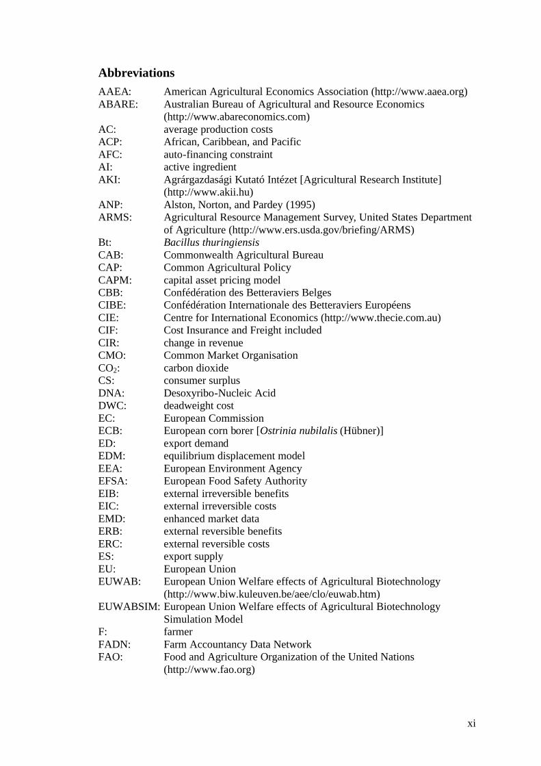
Abbreviations AAEA: American Agricultural Economics Association (http://www.aaea.org) ABARE: Australian Bureau of Agricultural and Resource Economics

(http://www.abareconomics.com) AC: average production costs ACP: African, Caribbean, and Pacific AFC: auto-financing constraint AI: active ingredient AKI: Agrárgazdasági Kutató Intézet [Agricultural Research Institute]

(http://www.akii.hu) ANP: Alston, Norton, and Pardey (1995) ARMS: Agricultural Resource Management Survey, United States Department

of Agriculture (http://www.ers.usda.gov/briefing/ARMS) Bt: Bacillus thuringiensis CAB: Commonwealth Agricultural Bureau CAP: Common Agricultural Policy CAPM: capital asset pricing model CBB: Confédération des Betteraviers Belges CIBE: Confédération Internationale des Betteraviers Européens CIE: Centre for International Economics (http://www.thecie.com.au) CIF: Cost Insurance and Freight included CIR: change in revenue CMO: Common Market Organisation CO2: carbon dioxide CS: consumer surplus DNA: Desoxyribo-Nucleic Acid DWC: deadweight cost EC: European Commission ECB: European corn borer [Ostrinia nubilalis (Hübner)] ED: export demand EDM: equilibrium displacement model EEA: European Environment Agency EFSA: European Food Safety Authority EIB: external irreversible benefits EIC: external irreversible costs EMD: enhanced market data ERB: external reversible benefits ERC: external reversible costs ES: export supply EU: European Union EUWAB: European Union Welfare effects of Agricultural Biotechnology

(http://www.biw.kuleuven.be/aee/clo/euwab.htm) EUWABSIM: European Union Welfare effects of Agricultural Biotechnology

Simulation Model F: farmer FADN: Farm Accountancy Data Network FAO: Food and Agriculture Organization of the United Nations

(http://www.fao.org)

xii

FAPRI: Food and Agricultural Policy Research Institute, University of Missouri (http://www.fapri.missouri.edu)

FOB: Free On Board G-7: Group of Seven (Canada, France, Germany, Italy, Japan, United

Kingdom, and United States) GARB: gross annual research benefits GC: gross production cost GDP: gross domestic product GE: genetically engineered GM: genetically modified GMO: genetically modified organism GTAP: Global Trade Analysis Project, Purdue University

(https://www.gtap.agecon.purdue.edu) HH: household HT: herbicide tolerant IFPRI: International Food Policy Research Institute (http://www.ifpri.org) INRA: Institut National de la Recherche Agronomique (http://www.inra.fr) IP: identity preservation, identity preserved IPR: Intellectual property rights IR: Insect resistant IRBAB: Institut Royal Belge pour l’Amélioration de la Betterave

(http://www.irbab.be) IRR: internal rate of return ISA: International Sugar Agreement ITB: Institut Technique Français de la Betterave Industrielle

(http://www.institut-betterave.asso.fr) L.: Linnaeus LDP: London Daily Price LSR: land supply response MAPA: Ministerio de Agricultura, Pesca y Alimentación (http://www.mapa.es) MC: market clearing MCB: Mediterranean corn borer [Sesamia nonagrioides (Lefebvre)] MLS: Moschini, Lapan, and Sobolevsky (2000) MR: marginal return MUV: Manufacturing Unit Value index NLCE: non-linear constant-elasticity NPV: net present value NY: New York OCQ: Oehmke and Crawford (2002) and Qaim (2003) OECD: Organisation for Economic Co-operation and Development

(http://www.oecd.org) OLS: ordinary least squares PIB: private irreversible benefits PIC: private irreversible costs PRB: private reversible benefits PRC: private reversible costs PS: producer surplus R&D: research and development ROR: risk-free rate of return ROW: rest of the world

xiii

RVW: rest van de wereld SE: standard error SIGMEA: Sustainable Introduction of Genetically Modified crops in European

Agriculture (http://sigmea.dyndns.org) soyb.: soybeans SME: small and medium enterprise SPEL: Sektorales Produktions- und Einkommensmodell der Landwirtschaft

[Sectoral Production and Income Model of Agriculture], European Commission (http://www.agp.uni-bonn.de/agpo/rsrch/spel/spel_e.htm)

TFP: total factor productivity UC Davis: University of California, Davis (http://www.ucdavis.edu) UK: United Kingdom USA: United States of America US: United States USDA: United States Department of Agriculture (http://www.usda.gov) VIB: Flanders Interuniversity institute for Biotechnology

(http://www.vib.be) WTP: willingness-to-pay ZEW: Zentrums für Europäische Wirtschaftsforschung [Centre for European

Economic Research] (http://www.zew.de)

xiv

1

Introduction1

The study of innovation in agriculture

The study of innovation has a long standing tradition in the field of agricultural economics. Particularly, the determinants of the adoption and diffusion of innovations go back a long while. In his seminal study on the adoption of hybrid corn in Iowa, Griliches (1957) developed an economic version of the S-shaped diffusion curve and confirmed that profitability gains positively affect adoption. Feder, Just, and Zilberman (1985) review a large body of empirical studies that originated in the work of Griliches. In a more recent paper, Sunding and Zilberman (2001) provide the most comprehensive overview of this literature to date. Studying the determinants of innovation usually involves studying its impact, since innovation only occurs when the impact for the farmer is positive. However, in recent years, studies focusing solely on the impact of innovations have emerged.

Agricultural research is conducted in the context of other economic and agricultural policies, but research is only one instrument of social policy, and most non-efficiency-related objectives are more effectively pursued using other policy instruments. Thus public-sector research should be treated as one of several available instruments for attaining agricultural-sector goals, and decisions on research resources should reflect the reasons behind public-sector involvement in research. In many places, stated objectives for the agricultural research system include (i) economic growth, (ii) income distribution, and (iii) food security. Environmental objectives are frequently voiced as well but can be thought of as falling under growth, distributional, and security objectives. For example, environmental concerns often arise when measures of growth fail to include the external costs associated with environmental damage or when the distribution of benefits to future generations may be jeopardised (Alston, Norton, and Pardey, 1995).

The basic model

Only by diffusion and on-farm adoption can agricultural innovations pass on benefits to society. Conventionally, research benefits were estimated assuming that the research is publicly funded and innovated inputs competitively sold in the input market. Figure 1a represents the output market of the farm sector. Let S0(p) be the

1 Parts of this introduction have been published in Demont, M., J. Wesseler, and E. Tollens. “Irreversible costs and benefits of transgenic crops: what are they?” Environmental costs and benefits of transgenic crops. Wesseler, J., ed., pp. 113-122. Dordrecht, NL: Springer, 2005 and in Demont, M., E. Mathijs, and E. Tollens. “Impact of New Technologies on Agricultural Production Systems: The Cases of Agricultural Biotechnology and Automatic Milking.” New Technologies and Sustainability. Bouquiaux, J.-M., L. Lauwers, and J. Viaene, ed., pp. 11-38. Brussels: CLE-CEA, 2001.

2

upward sloping supply curve and D(p) the downward sloping demand curve in the output market for the conventional agricultural commodity being modelled. The innovation is assumed to be cost reducing and/or yield enhancing, resulting in a shift of the supply curve from S0(p) to Sc(p) on the condition that the innovated input is competitively supplied. Consumers are better off because the R&D enables them to consume more of the commodity at a lower price. Producers are better off if their unit costs fall by an amount that exceeds the fall in price. As a result, the supply shift leads to an increase in economic welfare, which is the sum of the benefits accruing to consumers and producers and is equal to the area ABDE, the so-called gross annual research benefits (GARB). The GARB can be compared with the R&D investment costs (C) by calculating the internal rate of return (IRR). This is defined as the discount rate that yields a zero net present value (NPV) on time t:

0)1(0

=+

−= ∑∞

=

++

j jjtjt

IRR

CGARBNPV (1)

An investment that has NPV > 0, given a discount rate of i, will also have an IRR > 0. Thus, according to the IRR criterion, an investment is profitable if the computed IRR is greater than the required (market) rate of return: IRR > i.

p

y

S0(p ) S c(p )

B

A

C

F

w

x

c G

H

MR

X(w )

D(p )

(a) (b)

S m(p )

D

E

w1 /α

c /α

Change in Marshallian surplusInnovated inputsuppliers’ rent

x0 αx1

I

Figure 1: Change in Marshallian surplus (area ABCF or cGHw1/α) and innovated input suppliers’ monopoly rent (area w1/αHIc/α) resulting from an IPR-protected innovation in the input market The basic model presented in Figure 1a, has been used for numerous agricultural research evaluation and research priority studies (Alston, Norton, and Pardey, 1995). Recently, Alston et al. (2000) performed a meta-analysis of annual IRRs to agricultural R&D, compiling a comprehensive dataset of 292 publications representing the entire postwar history of quantitative assessment of IRRs to agricultural R&D. First, they find a large range of IRRs with an overall average of

3

65% and a standard deviation of 86% per year. Second, the authors find no evidence to support the view that the rate of return to research has declined over time. Thirdly, the IRR is higher when the research is conducted in more developed countries. Fourth, lower rates of return are found for natural resource management research (primarily forestry) and higher rates are associated with annual crops. The high payoffs suggest that agricultural research and extension have been very productive. This also means that had there been more funds for research, the returns would have been lower, i.e. the amount invested has been suboptimal, suggesting a permanent underinvestment in public research expenditures in agriculture (Roseboom, 2002).

Privately funded R&D protected by intellectual property rights

In Figure 1a, research benefits were estimated assuming that the research is publicly funded and innovated inputs competitively sold in the input market. However, most of the recent agricultural biotechnology innovations have been developed by private firms protected by intellectual property rights (IPR), such as patents, which confer monopoly rights to the discoverer (with some limitations). The result is that prices for these inputs are higher than they would be in a perfectly competitive market. Therefore, Moschini and Lapan (1997) bring along some new elements in the conventional analytical framework. They complete it by including the possibility that the innovation is protected by intellectual property rights in the input market. Thus, the correct evaluation of the benefits from R&D aimed at agriculture needs to account for the relevant institutional and industry structures responsible for the actual development of technological innovations.

The technology is assumed to be cost reducing and this can be visualised in the input market (Figure 1b) by representing input prices in efficiency units, resulting from a one-factor-augmentation model. This allows the new, more productive factor to be measured in the same physical units as the pre-innovation input. Farmers will adopt the new variety if the price in efficiency units of the new input is less than that

of the old input, i.e. w1/α ≤ c. In other words, farmers will adopt a biotechnology variety when the value of the cost reduction plus the increase in yield is greater than the price differential between these varieties. It is reasonable to assume that both types of seeds are produced at a constant marginal cost c. We also assume that the conventional technology is produced in a perfectly competitive input market, so that its price approximates its marginal cost c. However, in the case of the new technology, the intellectual property rights allow the firm to hold a temporary monopoly position, bounded of course by some limit (Lapan and Moschini, 2000).

Let X(w) be the downward sloping demand curve of the farm sector for genetically engineered seed (GE) in the input market (Figure 1b). The higher the price w, the lower demand x will be for the improved variety due to the existence of

4

alternative conventional technologies such as chemicals. If the firm is the only player in the market, it faces the demand curve X(w). The marginal return curve MR, or return of an additional unit seed sold on the market, can be easily derived from this demand curve (Figure 1b). The firm will maximise profits by producing an amount

GE seed equal to αx1, where marginal cost c/α in efficiency units is equal to marginal return MR. Since it is the only player in the market facing demand curve X(w), the

firm is able to raise its price above the marginal cost c/α. Even at a price w1/α , the

farm sector is willing to buy αx1 units of the GE seed variety. This monopoly price

w1/α will maximise firm profits and will allow the firm to regain the high R&D costs

via a so-called monopoly rent, represented by rectangle w1/αHIc/α. Because of the

fact that the monopolistic seed price w1/α is higher than the marginal cost c/α, i.e. the seed price that would emerge in a perfectly competitive market, farm-level benefits are lower and the corresponding supply shift is smaller.

The effects of a departure from the assumption of perfect competition towards monopoly are visualised in Figure 1a through a shift of the supply curve from Sc(p) to Sm(p). Hence, the Marshallian surplus increase equals area ABCF instead of area ABDE as in the conventional framework of Alston, Norton, and Pardey (1995). However, according to Moschini and Lapan (1997), welfare effects of IPR-protected

innovated inputs have to be estimated in the input market, with area cGHw1/α representing the change in Marshallian surplus. Thus, the correct estimation of total

welfare increase is equal to the sum of the shaded areas cGHw1/α and w1/αHIc/α.

Biotechnology innovations in agriculture2

The year 2005 marked the tenth anniversary of the commercialisation of genetically engineered crops. In 2005, the 400 millionth hectare of a GE crop was planted by one of 8.5 million farmers in one of 21 countries. Remarkably, the global GE crop area increased more than fifty-fold since GE crops were first commercialised in 1996. The global area of approved GE crops in 2005 was 90 million hectares (Figure 2). Notably, of the four new countries that grew GE crops in 2005, three were European Union (EU) countries, i.e. Portugal, France, and the Czech Republic. Portugal and France resumed the planting of Bt maize in 2005 after a gap of 5 and 4 years respectively, whilst the Czech Republic planted Bt maize for the first time in 2005. The 21 countries growing biotech crops included 11 developing countries and 10 industrial countries; they were, in order of acreage, USA, Argentina, Brazil, Canada, China, Paraguay, India, South Africa, Uruguay, Australia, Mexico, Romania, the

2 In this dissertation, we define biotechnology as ‘modern’ or molecular biotechnology, involving genetic engineering and the creation of transgenic plants. In our definition, beer brewing, fermentation or in vitro culture are not included.

5

Philippines, Spain, Colombia, Iran, Honduras, Portugal, Germany, France and the Czech Republic.

Figure 2: Global area of transgenic crops (1996-2005) The USA, followed by Argentina, Brazil, Canada and China continue to be the principal adopters of GE crops globally, with 49.8 million ha planted in the USA (55% of global GE area). GE soybean continues to be the principal GE crop (54.4 million ha at 60%), followed by maize (21.2 million ha at 24%), cotton (9.8 million ha at 11%) and canola (4.6 million ha at 5% of global GE crop area). Herbicide tolerance (HT), deployed in soybean, maize, canola and cotton continues to be the most dominant trait occupying 63.7 million ha (71%) followed by Bt insect resistance at 6.2 million ha (18%) and 10.1 million ha (11%) to the stacked3 genes. The latter was the fastest growing trait group between 2004 and 2005 at 49% growth, compared with 9% for herbicide tolerance and 4% for insect resistance (James, 2006).

Distributional issues

Since most of the recent agricultural biotechnology innovations have been developed by private companies, the central focus of societal interest is not on the rate of return to research, but on the distribution of the gains from these technologies among all

3 Crops with stacked genes contain two foreign genes of agronomical importance, e.g. herbicide tolerance and insect resistance.

6

stakeholders involved in the agribusiness chain, i.e. input suppliers, farmers, processors, distributors, consumers and government. A popular argument used by the opponents of agricultural biotechnology is the idea of the life science sector extracting all benefits generated by these innovations. The first ex post impact studies of agricultural biotechnology around the world indicate that farmers are clearly capturing sizeable gains of the new technologies. Table 1 suggests that the size and distribution of the welfare effects of transgenic crops are a function of (i) the adoption rate, (ii) the crop, (iii) the biotechnologically improved trait, (iv) the geographical region, (v) the year, (vi) national policies and IPR protection and (vii) the assumptions and the underlying dataset of the study. Rows 10 and 11 suggest that the global welfare effects of HT soybeans can diverge with a factor of 2.4, depending on the assumed value for the US soybean supply elasticity (see Chapter 4 for a theoretical explanation). Table 1: Global welfare distribution of the first generation of transgenic crops Country Crop Year Adoption Welfare Welfare distribution

(%) (m$) Domestic farmers

Innovators Domestic consumers

Net ROW

USA Bt cotton 1996 14% 134 43% 47% 6% 4% USA Bt cotton 1996 14% 240 59% 26% 9% 6% USA Bt cotton 1997 20% 190 43% 44% 7% 6% USA Bt cotton 1998 27% 213 46% 43% 7% 4% USAa Bt cotton 1996-98 20% 151 22% 46% 14% 18% USAb Bt cotton 1997 20% 213 29% 35% 14% 22% USAc Bt cotton 1997 20% 301 39% 25% 17% 19% USA HT cotton 1997 11% 232 4% 6% 57% 33% USAd HT soyb. 1997 17% 1,062 76% 10% 4% 9% USAe HT soyb. 1997 17% 437 29% 25% 17% 28% USA HT soyb. 1999 56% 804 19% 45% 10% 26% USA HT soyb. 1997 17% 308 20% 68% 5% 6% Canadaf HT canola 2000 54% 209 19% 67% 14% . Argentina HT soyb. 2001 90% 1,230 25% 34% 0.3% 41% Argentina Bt cotton 2001 5% 0.4 21% 79% . . China Bt cotton 1999 11% 95 83% 17% 0%g . India Bt cotton 2002 7% 6.2 67% 33% 0%g . Mexico Bt cotton 1998 15% 2.8 84% 16% . . South Africah Bt cotton 2000 75% 0.1 58% 42% . . South Africai Bt cotton 2001 80% 1.2 67% 33% 0%g 0% HT: herbicide tolerant, ROW: rest of the world, soyb.: soybeans a We calculated the 3-year average and subtracted the cost for taxpayers from the US consumer surplus. b based on the ARMS dataset; c based on the EMD dataset d assuming a low US soybeans supply elasticity of 0.22; e assuming a high elasticity of 0.92 f For consistency with the other estimates, the innovators’ share is based on gross rents and we subtracted 14% of consumer benefits of the estimated farmer benefits. g Due to governmental price support, demand is assumed infinitely elastic. h The study is geographically limited to the Makhatini Flats in KwaZulu-Natal. i The study is based on the entire country. For consistency with the other estimates, we omit the losses of pesticide companies. Sources: Falck-Zepeda, Traxler, and Nelson (1999, 2000a, 2000b), Moschini, Lapan, and Sobolevsky (2000), Pray et al. (2001), James (2002), Frisvold and Tronstad (2003), Phillips (2003), Price et al. (2003), Qaim (2003, 2005), Qaim and de Janvry (2003), Thirtle et al. (2003), Gouse, Pray, and Schimmelpfennig (2004), Qaim and Traxler (2005) and Traxler et al. (2003)

7

Regardless the variability of the welfare estimates, Table 1 reveals that, on average, one third of the global benefits (37%) is extracted by the innovators (gene developers and seed suppliers), while two thirds (63%) are shared among domestic and foreign farmers and consumers. This typical welfare partition of one third upstream4 versus two thirds downstream seems to be the general rule of thumb in the welfare distribution of the first generation of agricultural biotechnology innovations. Remarkable is also the fact that this rule of thumb seems to be valid for both industrial and developing countries. In developing countries, monopolistic rent creation by biotechnology companies is hampered by (i) weak IPR protection, (ii) governmental market protection and monopolisation and (iii) technical restrictions. In Argentina, for example, due to weak IPR protection there is a widespread use of farmer-saved and black market seed. This leads to downward pressure in conventional and GE seed prices and widespread adoption of GE seed. As a result, Argentine soybean growers capture 90% of the domestic benefits (Qaim and Traxler, 2005). In China, county and provincial seed companies’ monopoly on the sale of seeds prevents private and most other government enterprises from competing with them. In addition, international seed companies other than Monsanto have not been allowed to enter the Chinese seed market unless they are willing to be minority partners in a joint venture. Together with weak IPR protection, this leads to low or nonexistent royalties and large farmer benefits (Pray et al., 2001). Finally, since hybrids can only be reproduced with a notable decline in productivity, there is a technical restriction to use farm-saved seeds. As a result, contractual use restrictions, as a measure for IPR protection, prove to be effective for Bt cotton in Argentina, leading to higher price premiums for GE seed and higher rent extraction of multinational firms (Qaim, 2005).

All of the impact studies mentioned in Table 1 draw upon the analytical framework of Moschini and Lapan (1997). However, econometric estimation of the derived demand curve X(w) for GE seed in the input market (Figure 1b) would require data that are difficult to obtain. In particular, to analyse the impact of recent agricultural biotechnology innovations would require the use of cross-sectional data which are unlikely to contain sufficient price variability to obtain precise parameter estimates (Falck-Zepeda, Traxler, and Nelson, 2000b). Therefore, most of the studies estimate Marshallian surplus in the output market drawing on Alston, Norton, and Pardey (1995) and estimate the monopolistic rent of the input suppliers in the input market following Moschini and Lapan (1997).

4 In the literature, the monopoly rents of the innovators are calculated as gross technology revenues. No research, marketing or administration costs are deducted, because such data are not easily available. If these costs were deducted, the general rule of thumb could rather become ‘one quarter upstream and three quarters downstream’. For an example of a study incorporating such data, see Phillips (2003).

8

Regulatory issues

Somewhat paradoxically, the novelty of GE crops explains both the enthusiastic support of their proponents and the widespread consumer and public opposition that has hampered its adoption in many European and Asian importing countries. The response of these countries has been to develop relatively restrictive procedures for pre-market approval of GE crops and foods, and to require mandatory labelling of such foods (Sheldon, 2002). From October 1998 to May 2004, no GE crops have been approved for commercial release in the EU, and there were several applications pending approval at various stages in the procedure. In June 1999, five member states (Denmark, Greece, France, Italy, and Luxembourg) signed a declaration stating they would block any further approvals until a revised Directive on labelling, traceability and liability would come into force (Bijman and Tait, 2000). This de facto moratorium on the approvals of new GE crops, brought into effect by EU governments since 1998, claimed the adoption of the precautionary principle by the European Parliament meeting public concerns (environmental impact and public health safety) on transgenic crops. As European legislation had been developed (Directive 2001/18/EC5, Guidelines on coexistence6, Regulation (EC) 1830/20037 and Regulation (EC) 1829/20038), the de facto moratorium officially ended in May 2004 with the authorisation to import transgenic sweet maize (Bt 11, patented by the seed company Syngenta) for food use (Messéan et al., 2006).

Despite the official end of the moratorium and new approvals of GE crops, adoption of national guidelines on coexistence has been relatively slow and due to regulatory uncertainty and consumer hostility, the adoption of GE crops is still limited. At present, the only significant use of transgenic crops in the EU is the cultivation of GE insect resistant maize in Spain (see Chapter 3). This means that the EU is still in a state of quasi-moratorium regarding the introduction of GE crops, foregoing important benefits of these new technologies.

5 Directive 2001/18/EC of the European Parliament and of the Council of 12 March 2001 on the deliberate release into the environment of genetically modified organisms and repealing Council Directive 90/220/EEC-Commission Declaration. 6 Commission Recommendation 2003/556/EC of 23 July 2003 on guidelines for the development of national strategies and best practices to ensure the coexistence of genetically modified crops with conventional and organic farming. 7 Regulation (EC) No. 1830/2003 of the European Parliament and of the Council of 22 September 2003 concerning the traceability and labelling of genetically modified organisms and the traceability of food and feed products produced from genetically modified organisms and amending Directive 2001/18/EC. 8 Regulation (EC) 1829/2003 of the European Parliament and of the Council of 22 September 2003 on genetically modified food and feed.

9

Externalities

While the benefits of agricultural biotechnology have been widely demonstrated in literature (Table 1), the quasi-moratorium on transgenic crops in Europe is primarily based on consumer concerns about the safety of these crops with respect to possible long-term adverse effects on the environment and human health but also on doubts on the sustainability of this new agricultural technology and on the impacts that its adoption might have on global agro-food production and society at large. These so-called externalities are not included in the conventional welfare frameworks that demonstrate the benefits of GE crops in Table 1.

Therefore, in this dissertation, we design a two-dimensional matrix defining four quadrants of research for the ex ante assessment of transgenic crops (Figure 3). The scope dimension distinguishes between market (private) effects and non-market (external) effects. Reversibility refers to non-additional benefits or costs, after an action has stopped. If a farmer stops planting sugar beets, he can use the fertiliser he bought for other crops and reverse the costs. At the external level, the damage on honeybees can be reversed if harmful pesticides are banned. In both examples, reversing the action does not include sunk costs. Irreversibility refers to additional benefits or costs, after an action has stopped. If a farmer stops planting sugar beet and has to sell his sugar beet harvester, he may receive a lower price after depreciation and may be unable to reverse all the costs.

Research Quadrant 1 is mainly focused on producer and consumer surplus changes. Private reversible benefits (PRB) of GE crops comprise pecuniary benefits, such as yield increase and pest control cost decrease as well as non-pecuniary benefits such as management savings, enhanced flexibility and convenience (see Chapter 5). The higher monopolistic price of GE seed translates into a private reversible cost (PRC) for the farmer. The release of HT sugar beet may have a negative impact on long-term biodiversity9 resulting in external irreversible costs (EIC) as discussed in Chapter 2. At the same time, a reduction of pesticide use in HT sugar beet may have a positive impact on farmer’s health, i.e. a private irreversible benefit (PIB), on field biodiversity and society as a whole, i.e. an external irreversible benefit (EIB) (Antle and Pingali, 1994, Waibel and Fleischer, 1998). Hence, the release of transgenic crops produces not only irreversible costs but also irreversible benefits, a term introduced by Pindyck (2000) in the context of greenhouse gas abatement. A complete ex ante analysis of economic benefits and costs of transgenic crops should consider all four quadrants of research, depicted in Figure 3.

9 In the discussion on transgenic crops and biodiversity, one has to make a distinction between field biodiversity, i.e. the number and diversity of living organisms in a cultivated field, and long-term biodiversity resources for society, i.e. the number of cultivated species, the number of cultivars within the species and genetic reserves of cultivated plants, maintained in gene banks.

10

Scope

Reversibility

Private

External

Reversible

Quadrant 1

Private Reversible Benefits (PRB) Private Reversible Costs (PRC)

Quadrant 2

External Reversible Benefits (ERB) External Reversible Costs (ERC)

Irreversible

Quadrant 3

Private Irreversible Benefits (PIB) Private Irreversible Costs (PIC)

Quadrant 4

External Irreversible Benefits (EIB) External Irreversible Costs (EIC)

Figure 3: Two dimensions in an ex ante analysis of social benefits and costs of transgenic crops Whereas the first published ex post studies all concentrate on Quadrant 1 (Table 1), the other research quadrants remain poorly covered. Quadrant 3 and 4 include irreversibilities, which are important for ex ante studies. The few published ex ante studies on the impact of transgenic crops either only looked at net private reversible benefits, e.g. Qaim (1999), or did not include irreversibility, e.g. O’Shea and Ulph (2002). Hence, after a decade of worldwide experience with commercial biotechnology applications, an important research gap remains largely unfilled. In this dissertation, we undertake an initial attempt to approach the problem by focusing on Quadrant 1 (Chapter 1, 3, 4 and 5) and Quadrant 3 (Chapter 2).

Objective

The main objective of this dissertation is to contribute to the literature on the impact of transgenic crops and on returns to research estimations and to support and inform the policy debate on transgenic crops. First, we develop an ex ante welfare model for the assessment of the potential welfare effects foregone, due to the 1998 de facto moratorium, of a relevant biotechnology innovation in the EU-15. Secondly, we develop an ex ante decision model and use the data generated by the first model to reassess whether the approval of the technology in the EU should have been delayed or not, taking into account uncertainty and irreversibility of environmental costs. Thirdly, we develop a model to conduct the first ex post impact study of a biotechnological innovation in EU agriculture. Finally, we use the data generated by the third model to algebraically harmonise and empirically juxtapose five equilibrium displacement models commonly used in the literature, providing insights for returns to research estimation and stochastic equilibrium displacement modelling.

Hypotheses

The EU has chosen the option to wait through the 1998 moratorium and the current slow coexistence regulation process, postponing the release of GE crops. This option

11

has a value and a cost. Waiting pays as the veil of uncertainty will be removed year after year, but at the same time the benefits that could have been captured during this period are foregone. It is widely cited that the EU has to make science-based decisions on the release of transgenic crops. A decision which is based on the assumption that the risk cannot be estimated and therefore transgenic crops should not be released, implicitly assumes that the expected risks are higher than the expected benefits. Therefore, the trade-off of both need to be assessed in order to know the ex post implications of the decision in the past and in order to know the ex ante implications of future decisions, e.g. for new GE trait authorisations. In this dissertation, we will examine the following four hypotheses: Hypothesis 1: The first generation of agricultural biotechnology innovations could

and can significantly contribute to productivity and welfare in EU agriculture;

Hypothesis 2: The largest share of total welfare creation is captured downstream (farmers, processors, manufacturers, distributors and consumers);

Hypothesis 3: Conventional benefit-cost analysis cannot capture uncertainty and potential irreversibility regarding environmental effects. It can be extended by a real option approach to assess maximum tolerable levels of irreversible environmental costs that justify a release of these innovations in the EU;

Hypothesis 4: Some of the variability of welfare estimates reported in literature can be explained by the modelling of supply shift in conventional equilibrium displacement models.

Selection of case studies

The successful achievement of the main objective crucially depends on the selection of representative case studies. Instead of transferring the existing US studies presented in Table 1 and reproducing them in EU conditions, we opted for case studies that would better reflect European conditions of agriculture and agricultural trade. Therefore, we identified seven criteria for an EU case study to be successful:

1. Representativeness of the crop in EU agriculture; 2. Representativeness of the agronomic constraint in EU agriculture; 3. Representativeness of the crop or its refined product in EU and world trade; 4. Availability of genetic resources of the crop in EU agriculture; 5. Realistic acceptance of the GE variety; 6. Realistic commercialisation of the GE variety; 7. Availability of impact data, e.g. field or farm-scale trials.

The selection of a case study involves the selection of a crop, which has to be representative in acreage and income for European agriculture as a whole as well as

12

for individual EU-15 Member States. The agronomic constraint, for which the GE variety provides a solution, has to be representative for EU agriculture, e.g. pests such as lepidopterans or weeds. To assess the impact of EU adoption of GE crops on the world market, the crop or its refined product has to be an important export commodity. As a fourth criterion, a case study preferably focuses on a crop for which Europe is the primary centre of origin. In primary centres of origin, an abundance of genetic resources of the crop is available and environmental effects such as gene flow to wild relatives and the question of biodiversity become significant issues that are worthwhile to study. Moreover, the acceptance of the GE variety has to be realistic and near commercialisation. Finally, preferably a GE crop should be chosen for which impact data are available. The impact data can stem from field trials or, preferably, farm-scale trials. However, due to the de facto moratorium, data from the latter are scarce in the EU.

Table 2: Accordance of selected EU case studies on the impact of GE crops with criteria

Crop Criterion

HT sugar beet Bt maize

1. Representativeness of the crop +++ grown in all EU

regions

+ grain maize more important in southerly

regions 2. Representativeness of the pest +++

weed control is crucial to profitability

+ corn borers more important in southerly

regions 3. Representativeness of trade +++

EU provides 20% of global trade

– EU-15 and EU-25 are net importers of

maize, only internal EU trade 4. Availability of genetic resources +++

presence of wild relatives, e.g. sea beet

– no wild relatives in Europe,

primary centre of origin is Mexico 5. Realistic acceptance –

main impediments are manufacturers

+++ widely accepted in Spain, entirely used for animal feed, no labelling required

6. Realistic commercialisation ++ registrations are

pending

+++ already commercialised in Spain,

France, Germany, Portugal and the Czech Republic

7. Availability of impact data + research capacity has declined since 2001

+ very little data publicly available

Remarkably, the list of criteria suggests that the available US case studies (Table 1) largely fit the requirements, while not a single suitable EU case study can be found that fulfils all of the seven criteria. Therefore, we decided to select two case studies covering different parts of the criteria list. First, in selecting the case studies, we can not get around choosing the case of insect resistant Bt maize in Spain, providing the only ex post evidence available of a biotechnological innovation in EU agriculture. As a second case study, we chose a drastic innovation in a typical European crop, i.e. HT

13

sugar beet. Both case studies also cover the two most important traits of the first generation of GE crops, i.e. herbicide tolerance and insect resistance. In Table 2 we check the accordance of our selected case studies with the postulated criteria.

The case of HT sugar beet is very appealing for EU agriculture as this crop is grown in all EU countries and the EU is an important player on the world sugar market10 (Table 3 and Table 4 in Chapter 1). Moreover, weed control is crucial to economic beet production. Sugar beet is a typical European crop and has wild relatives in Europe, e.g. the sea beet, Beta vulgaris subsp. maritima (Santoni and Bervillé, 1992, Bartsch et al., 1999). Therefore, gene flow to wild relatives and preservation of biodiversity are crucial factors of the long-term sustainability of sugar beet cultivation (Chapter 2). In 1999, when the case studies were selected for the EUWAB project we initially believed that the acceptance of HT sugar beet would be realistic as sugar does not contain any proteins nor DNA and would not have to be labelled (Duff, 1999, p. 6). However, since nowhere in the world transgenic sugar beets have been adopted, we understood that the major impediment comes from the concentrated group of refiners, processors and manufacturers of sugar and sugar-containing products. Processors face risks related to market acceptability of sugar and by-products such as pelletised pulp, which is sold in international markets like Europe and Japan (DeVuyst and Wachenheim, 2005). US manufacturers are not willing to accept GE sugar even though they have no safety concerns and recognise that it would be difficult to guarantee they are not using any other GE products (Kilman, 2001).

As a result, in the EU, registrations of GE sugar beet varieties, field trials (Figure 4) and research capacity have been gradually phased out since 1998. The moratorium resulted in EU product approval (Part C) for commercial cultivation for glyphosate tolerant sugar beet being stalled in early 1999. Monsanto also applied for novel foods approval for foods and food ingredients derived from Roundup Ready sugar beet. The initial assessment report is still pending (PG Economics Ltd., 2003).

The acceptance of Bt maize on the other hand is very realistic. Being currently adopted in Spain, France, Germany, Portugal and the Czech Republic, it is expected that this GE crop will be the first to be grown in European regions where the European corn borer and Mediterranean corn borer are important pests (Devos, Reheul, and De Schrijver, 2005). Since these pests are mainly representative for grain maize, the innovation is mainly of interest for Southern Europe. Finally, despite the commercial scale of adoption, at the time of conducting the Bt maize impact study in Spain in 2002, very little impact data was available.

10 It is important to note that this is an artificial situation in a sense, engendered by high, protected prices and quotas in the EU sugar beet industry and preferential sugar import agreements with developing countries.

14

0

10

20

30

40

50

60

70

80

90

1991 1992 1993 1994 1995 1996 1997 1998 1999 2000 2001 2002 2003 2004

Maize Sugar beet

Figure 4: Evolution of the number of field trials of maize and sugar beet in the EU-25 Source: SNIF database (European Commission, 2006a)

Delimitation of the study

The study field of this dissertation can be defined according to four dimensions: 1. Geographical dimension: the EU-15 and Spain are analysed; 2. Temporal dimension: 1996-2003, i.e. post-introduction and pre-coexistence; 3. Crops: sugar beet (Beta vulgaris L.) and maize (Zea mays L.); 4. Biotechnological traits: herbicide tolerance (HT) and insect resistance (Bt).

The analysed geographical region is the EU-15, i.e. the decision-maker of the 1998 de facto moratorium on transgenic crops. As of May 1st, 2004, 10 new Central and Eastern European Member States joined the EU, i.e. Cyprus, Czech Republic, Estonia, Hungary, Latvia, Lithuania, Malta, Poland, Slovakia and Slovenia. These countries are not explicitly modelled in this dissertation. In the framework of the EUWAB project however, we conducted case studies on the impact of transgenic crops (maize, sugar beet and oilseed rape) in two New Member States, i.e. Hungary and the Czech Republic. The publications are available on the EUWAB website.

The definition of a counterfactual scenario is a necessary prerequisite for any ex ante analysis. For HT sugar beet, we analyse the first phase of the introduction of the first generation of GE crops, i.e. from 1996 to 2001, and hypothetically assume adoption in the EU. This means that the counterfactual scenario is entirely embedded in the pre-coexistence period, i.e. before the implementation of the new labelling and traceability regulations in April 2004 and the Guidelines on coexistence (still under discussion). However, research is currently being undertaken at the farm level impact of these regulations under the European Commission 6th Framework SIGMEA project (Sustainable Introduction of Genetically Modified crops in European Agriculture).

15

Secondly, the counterfactual scenario takes place under the former EU Common Market Organisation (CMO) for sugar. In the framework of the EUWAB project, research has been initiated on reproducing the study under the future conditions of the new CMO for sugar, which will be implemented in July 2006 (European Commission, 2005). In Chapter 5, we graphically and algebraically analyse how the new CMO will affect our results. Nevertheless, the period from 1996 to 2001 is the most relevant counterfactual period to study, as field trials and research efforts on GE sugar beet have been significantly cut back since 2001 (Figure 4). Moreover, incorporating an historical part in our analysis draws the attention to the potential benefits, benefits forgone or costs of the 1998 de facto moratorium on transgenic crops in the EU. The ex post analysis, finally, is based on the introductionary phase of Bt maize in Spain, i.e. from 1998 to 2003.

Most of the work in this dissertation has already been published in international peer reviewed journals or books (see Publication list). However, since their publication, we have updated our data and assumptions with new information and insights, refined our models with more sophisticated modelling techniques and added new analyses. Therefore, the results presented in this dissertation are original and slightly differ from the published articles, although without changing any of the general qualitative findings. As the chapters presented in this dissertation are strongly interlinked, we considered this as an essential step in the accomplishment of this work. Consequently, the results we present in one chapter can not be disconnected from the results obtained in the previous chapters.

16

17

Chapter 1: Ex ante welfare effects of agricultural biotechnology in the EU-15: The case of transgenic herbicide tolerant sugar beet1

Introduction

In the USA, the first published ex post welfare studies reveal the distribution of the benefits from agricultural biotechnology (Table 1). The studies are applied on typical US export crops such as cotton and soybeans. However, with the exception of two studies, using the GTAP (Global Trade Analysis Project, Purdue University) model to assess the global trade and/or welfare effects of the European Union (EU) moratorium on GE crops (Nielsen and Anderson, 2001, van Meijl and van Tongeren, 2004), and one case study on Ireland, based on farm level gross margin comparisons (Flannery et al., 2004), no comparable ex ante study has yet been published for the EU.

Sugar

Sugar is one of the most heavily protected agricultural commodities, implying for our study that these market interventions distort the flow of benefits from R&D in agriculture, such as biotechnology research. However, the sugar industry is facing a slow but steady progress towards greater liberalisation of global trade. Over the last 40 years, real world sugar prices have fallen, on average, by between 1.5% and 2.0% per year (Duff, 1999). Even in the case of the highly protected European beet industry, growers are paid a fixed ‘green rate’ price, i.e. not corrected for inflation. This means that they have to compete continuously against an annual real price decline of 1.9% via technological progress. This is actually the only way benefits of technological progress end up being passed on to EU consumers (Thirtle, 1999).

These arguments provide a powerful economic rationale for enhancing competitiveness by exploiting any cost savings that can be achieved, e.g. through the use of biotechnology. However, although most European countries have sufficient research experience in genetically engineered (GE) sugar beet, no authorisation or commercialisation of these crops is expected soon. Nowhere in the world has transgenic sugar beet been adopted on a commercial scale yet. This justifies the elaboration of an ex ante study about the potential welfare effects of agricultural biotechnology in the EU-15 sugar sector.

1 We would like to express our gratitude to Julian M. Alston (UC Davis), Giancarlo Moschini (Iowa State University), Brent Borrell (CIE, Canberra) and Ivan Roberts (ABARE, Canberra) for reviewing a previous version of this chapter with previous results, published as: Demont, M., and E. Tollens. “Ex ante welfare effects of agricultural biotechnology in the European Union: The case of transgenic herbicide tolerant sugarbeet.” The regulation of agricultural biotechnology. Evenson, R.E., and V. Santaniello, ed., pp. 239-255. Wallingford, UK: CAB International, 2004.

18

Table 3: World sugar production and utilisation (in thousand tonnes), average 1996-2000 Raw Sugar Beet Cane Total % Export % Net export Change stocks Cons. EU-15 18,406 9 18,415 14 8,398 20 3,790 -10,475 14,261 Eastern Europe 7,984 0 7,984 6 1,611 4 -6,385 193 14,177 Other West. Europe 3,137 0 3,137 2 425 1 -151 10,997 3,112 USA 4,056 3,126 7,181 6 226 1 -1,747 169 9,081 Japan 662 180 841 1 6 0 -1,588 -76 2,506 Canada 121 0 121 0 19 0 -1,108 -1 1,230 Australia 0 5,311 5,311 4 3,975 10 3,972 44 1,103 Brazil 0 17,517 17,517 13 8,356 20 8,356 189 9,293 India 0 16,959 16,959 13 457 1 -46 475 16,525 Indonesia 0 1,913 1,913 1 7 0 -1,507 110 3,243 Mexico 0 5,102 5,102 4 645 2 583 23 4,501 South Africa 0 2,628 2,628 2 1,249 3 1,152 78 4,070 Thailand 0 5,391 5,391 4 3,457 8 3,457 122 1,813 Other Central Am. 0 8,600 8,600 7 5,728 14 5,220 127 2,954 Other South Am. 483 6,270 6,753 5 1,687 4 592 152 6,012 Other Africa 623 5,901 6,524 5 2,487 6 -3,603 356 7,215 Other Asia 1,962 13,418 15,380 12 2,687 6 -8,955 192 24,151 Other Oceania 0 414 414 0 348 1 76 21 309 World 37,433 92,738 130,171 100 41,767 100 2,107 2,696 125,556 Source: F.O.Licht (2001) Table 4: World area and production of sugar beets and beet sugar, average 1996-2000 Country Area

(kha) % Beet prod.

(kt) % Yield

(t/ha) Sugar yield

(% white sugar) Sugar prod.

(kt white sugar) %

Austria 47 1 2.969 1 63 16 476 1 Belgium 96 1 5.927 2 62 16 960 3 Denmark 63 1 3.369 1 54 16 532 2 Finland 33 1 1.108 0 33 14 153 0 France 440 7 31.259 12 71 14 4.410 13 Germany 480 7 26.480 10 55 16 4.211 12 Greece 45 1 2.663 1 59 11 286 1 Ireland 33 1 1.708 1 52 13 217 1 Italy 270 4 12.958 5 48 12 1.606 5 Netherlands 114 2 6.531 3 58 15 1.012 3 Portugal 6 0 361 0 58 15 53 0 Spain 137 2 8.110 3 59 14 1.136 3 Sweden 58 1 2.592 1 45 16 407 1 UK 184 3 9.786 4 53 15 1.475 4 EU-15 2.005 31 115.819 46 58 15 16.934 49 Hungary 69 1 2.973 1 43 15 432 1 Czech Rep. 74 1 3.244 1 44 15 488 1 Poland 368 6 13.951 5 38 15 2.044 6 Russia 761 12 13.697 5 18 11 1.500 4 Ukraine 879 14 15.188 6 17 13 1.975 6 Turkey 434 7 17.939 7 41 13 2.289 7 Other 443 7 12.580 5 29 12 1.503 4 Europe 5.034 78 195.391 77 39 14 27.165 79 USA 568 9 27.959 11 49 13 3.731 11 China 406 6 11.410 4 28 10 1.103 3 Iran 178 3 4.784 2 27 12 564 2 Other 292 5 14.718 6 37 13 1.875 5 ROW 4.474 69 138.443 54 31 13 17.505 51 World 6.479 100 254.263 100 39 14 34.438 100 Sources: F.O.Licht (2001), FAO (2006)

19

Transgenic sugar beets

Effective weed control is essential for economic sugar beet production in all growing areas of the world. This was recognised as soon as the crop was first grown. The postemergence herbicides glyphosate and glufosinate-ammonium provide a broader spectrum of weed control in sugar beet than current systems, while at the same time reducing the number of active ingredients. The post-emergence herbicides glyphosate and glufosinate-ammonium provide a broader spectrum of weed control than current herbicide programs, while at the same time reducing the number of active ingredients. Glyphosate was first introduced as an herbicide in 1971. The gene that confers tolerance to glyphosate was discovered in a naturally occurring soil bacterium. Glufosinate-ammonium was discovered in 1981. The gene that confers tolerance to glufosinate is also derived from a naturally occurring soil bacterium. By inserting these herbicide tolerance (HT) genes into a plant’s genome, two commercial transgenic HT systems resulted: the Roundup Ready® system, providing tolerance to glyphosate and the Liberty Link® system, tolerant to glufosinate-ammonium.

These combinations of transgenic seed combined with a post-emergence herbicide, offer farmers broad-spectrum weed control, flexibility in the timing of applications, and reduce the need for complex compositions of spray solutions. For most growers, this translates into cheaper weed control. Moreover, these innovations are entirely coherent with the ongoing trend towards post-emergence weed control and reduced tillage techniques and the sharpening of the legal constraints for the application of herbicides (Schäufele, 2000). Both herbicides have a low toxicity and metabolise fast and without residues in the soil. Hence, the introduction of herbicide tolerant (HT) sugar beet varieties could be an approach to sustainable sugar beet cultivation (Märländer and Bückmann, 1999).

The model

To analyse the welfare effects of the adoption of HT sugar beet in the sugar industry, we need to choose an appropriate spatial model. Therefore, a preliminary look at the geographical distribution of production and trade of sugar is in order. Table 3 above reports the average global production and utilisation of sugar during 1996-2000. A differentiation into sugar cane and sugar beet appears logical, accounting for respectively 71% and 29% of global sugar production. The sugar beet region can be further divided into the EU-15 and the Rest of the World (ROW), both responsible for half of global beet sugar (Table 4 above). In this ROW beet region, non-EU-15 Europe is dominant (58%), followed by the USA (21%). Hence, we believe that we can adequately capture the essence of production and trade in the global sugar market with a three-region model: EU, ROW beet, and ROW cane.

20

Conventionally, research benefits were estimated assuming that the research is publicly funded and innovated inputs competitively sold in the input market. In contrast, most of the recent agricultural biotechnology innovations have been developed by private firms protected by intellectual property rights (IPR), such as patents, which confer monopoly rights to the discoverer. Monopolistic prices are higher than competitive ones. Therefore, Moschini and Lapan (1997) complete the conventional framework by including welfare measurement in the input market (Figure 1). However, in a more recent paper Moschini, Lapan and Sobolevsky (2000) adapt their methodology to a model that is closer to the actual working of the herbicide tolerance innovation and apply it to the case of Roundup Ready® soybeans. Our model is inspired by the latter. The spatial dimension is defined by 16 regions i: the ROW cane (i = 0), the ROW beet (i = 1), and 14 production blocks in the EU-15 (i = 2, …, 15). Belgium and Luxembourg are united in one block. The temporal dimension includes seven agricultural seasons j: one ‘benchmark year’ 1996/97 (j = 0) without adoption, five sequential years of adoption 1996/97, …, 2000/01 (j = 1, …, 5), and one ‘evaluation year’ 2001/02 (j = 6) to which the welfare effects are actualised and aggregated. Average profit per hectare is modelled through four terms: (i) a constant, (ii) a fixed per-hectare technology-induced profit increase, (iii) a yield effect, and (iv) a seed price effect (Moschini, Lapan, and Sobolevsky, 2000):

)1(1

)1(),( 1,

,, iii

jiiijiji wp

GAp i ρµδ

η

ρβραρπ η +−

+

+++= + (1)

Structural parameters Technology-specific supply shifters p = sugar price A, G = 16x6 matrices of parameters subsuming all other input prices, presumed constant η = 16x1 vector of elasticities of yield with respect to sugar price δw = 16x1 vector of seed costs (δ = constant optimal density of seeds and w = seed price) θ = 16x6 matrix of elasticities of land supply with respect to sugar profit per hectare

α = 16x1 vector of coefficients of unit profit increase due to the HT technology β = 16x1 vector of coefficients of yield change due to the HT technology ρ ∈ [0,1] = adoption rate µ = 16x1 vector of mark-ups on HT seed price (reflecting technology fee)

Supply of land to the sugar industry by country i in year j is written in constant-elasticity form as a function of average land rents, which depend on output price and the adoption rate:

),()],([)],([ ,,,,,, ρρπλρπ θ pLppL jijijijiji

ji == (2)

with λ = 16x6 matrix of scale parameters. The (optimal) yield function can be modelled as:

ipGpy jiijiηρβρ ,, )1(),( += (3)

Multiplying the land supply function by the yield function results in a region- and year-specific supply function incorporating four technology-specific parameters,

21

acting as shifters and enabling parameterisation of the herbicide tolerance innovation in detail:

ijii pGwpG

ApQ jiiiii

jiiijijiji

ηθη ρβρµδη

ρβραλρ ,

1,,,, )1()]1(

1

)1([),( , ++−

+

+++= +

(4) Aggregation of supply functions will allow us to model the effect on world sugar prices of the interaction between two aggregate blocks, the EU and the ROW, as a consequence of the introduction of the HT technology. However, the structure of these functions implies that all 16 regions in the model are able to participate in the aggregate supply response to prices. While all regions certainly respond to a certain region-specific ‘incentive price’, in reality not all of them respond to (lower) world prices, owing to price interventions interfering in their domestic market.2 This means that the technology-induced production surplus of those regions will not be exported on the world market, but will free up land allocated to sugar beets instead, so that their total production remains unchanged3. For those regions, we include this possibility by equalling their supply functions to their (constant) observed total production:

jiji QpQ ,, ),( =ρ (5)

Their land supply functions can then be modelled as:

),(),(

,

,, ρ

ρpy

QpL

ji

jiji = (6)

For regions i responding to world prices, we parameterise the supply function of HT sugar beet using Equation 4. All quantities and prices are converted to their white sugar equivalent. The aggregate EU sugar supply function in year j can be modelled

by imputing the country- and year-specific adoption rates ρi,j in the variable ρ and adding up all country-specific supply functions.4 Note that this aggregate supply function contains a constant and a variable term, which is a function of the world price:

),(),(),( ,,,,

15

2,,EU,EU jijijiji

ijijj pQQpQpQ ρρ ∑∑∑ +==

=

ρ (7)

In Equation 7, ρEU,j represents the 14x1 adoption vector of the new technology in the

EU in year j, with elements ρi,j (i = 2, 3, …, 15). This aggregate sugar supply function

2 We are grateful to Brent Borrell (CIE, Canberra) for pointing this out. 3 In the short run, these surpluses will be added to the carry-over and ‘precautionary’ production to ensure quota fulfillment. In the medium and long run, farmers will adapt their land allocated to sugar beet production. 4 According to Gohin and Bureau (2006), various world sugar market liberalisation studies produce inconsistent results because of the incorrect modelling of EU supply response. Therefore, using an aggregate function that summarizes heterogeneous individual behaviours is one way to deal with the problem.

22

is very detailed in that it contains 10 parameters per country, totalling 140 parameters, of which 56 are related to the new technology. In an analogous way, ROW aggregate supply can be modelled as a function containing a constant and a variable term:

),(),(),( ,,,,

1

0,,ROW,ROW jijijiji

ijijj pQQpQpQ ρρ ∑∑∑ +==

=

ρ (8)

In Equation 8, ρROW,j represents the 2x1 adoption vector of the new technology in the

ROW in year j with elements ρi,j (i = 0, 1). The 16x1 adoption vector in the whole

world in year j is denoted by ρW,j, containing elements ρi,j (i = 0, 1, …, 15). Next, we model the innovation as occurring in a large, open economy with technology spillovers and shape the two-region framework of Alston, Norton, and Pardey (1995, p. 219) to the specific features of the EU’s Common Market Organisation (CMO) for sugar. In Figure 5 the framework is represented. For each country, the four technology-specific parameters engender a pivotal, divergent shift of the supply curve. At the centre of the analysis is the calculation of a counterfactual world price pj (after decline) in year j to isolate the effect of the technology-induced supply shift from other exogenous changes in supply and demand. This price change differs from the observed change in world price if the technology is adopted as assumed. It rather represents what the world price would be if all supply and demand conditions are identical except for the introduction of the new technology (Falck-Zepeda, Traxler, and Nelson, 2000b). Hence, in our analysis we represent the world

price as a function of the worldwide adoption vector: pj(ρW,j). We assume a constant-elasticity EU demand function for sugar:

jppD jj,EU

,EU,EU )( εκ −= (9)

The EU’s export supply curve in year j can then be modelled as:

jjjjjjjj CpQpDpQpES −=−= ),()(),(),( ,EU,EU,EU,EU,EU,EU ρρρ (10)

with Cj the fixed consumption level in year j, due to fixed annual intervention prices.

The world price reduction (from pj(0) to pj(ρW,j) in Figure 5) is a synergy of

two forces. First, the EU’s export supply expansion (from ESj(p,0) to ESj(p,ρEU,j)), due to a technology-induced pivotal shift of the EU’s aggregate supply function (from

QEU,j(p,0) to QEU,j(p,ρEU,j)), would cause the world price to decline from pj(0) to

pj(ρEU,j). This price decrease can be determined using a reduced form equation, extracted from the of the University of Missouri’s Food and Agricultural Policy Research Institute (FAPRI) world sugar model, which calculates the world sugar price as a function of actual and lagged EU net sugar exports (Poonyth et al., 2000). By taking the first differential, and if we assume that imports are not affected by the innovation, due to fixed ACP (African, Caribbean, and Pacific) import agreements, we can calculate the world price as a function of the EU’s export supply expansion.

23

Figure 5: Distribution of R&D benefits in the EU’s sugar sector with technology spillovers to the rest of the world (ROW)

pp

p

qq

q

QEU,j(p,0)

(a) E

U q

uant

ity

(b) T

rade

d qu

anti

ty(c

) RO

W q

uant

ity

p j(0

)

Qa

D EU,j(p)

C

dc

b

ef

g

a

∆PS E

U,j

= b

–a

+ d

–c

≥0

∆CS E

U,j

= 0

∆PS E

U,j

= b

–a

+ d

–c

≥0

∆CS E

U,j

= 0

∆PS R

OW

,j=

g –

e ≤

0

∆CS R

OW

,j=

e +

f >

0

∆PS R

OW

,j=

g –

e ≤

0

∆CS R

OW

,j=

e +

f >

0

Qb

Qc,

0Qc,

1

Qc,

0Qc,

1

Qe,

0

Qe,

1

Qd

= Q

a+

Qb

–C

aQEU,j(p,ρEU,j)

ESj(p

,0)

ES j

(p,ρ

EU,j)

EDj(p

,0)

EDj(p

,ρR

OW

,j)

QR

OW

,j(p,

0)Q

RO

W,j(

p,ρ R

OW

,j)

DR

OW

,j(p)

p j(ρ

EU,j)

p j(ρ

W,j)

pa i,j(p

j(ρW

,j))

pb i,j(p

j(ρW

,j))

pi EU,j

pb i,j(p

j(0))

24

For each year j the model transforms the observed world price into the price that would result from the EU’s technology-induced export expansion in year j and j – 1:

−+=

)0),0((

)0),0(()),0((1)0()( ,EU

1,EUjj

jjjjjjjj pES

pESpESpp

ρσρ

(11)

−+

−−

−−−−−

)0),0((

)0),0(()),0((

11

111,EU112

jj

jjjjj

pES

pESpES ρσ with σ1 = -1.0 and σ2 = 0.46

The short-run flexibility σ1 is -1 and the long-run flexibility is approximately half that

of the short-run (σ1 + σ2 = -0.54), reflecting sugar export demand elasticities that are twice as large in the long run as in the short run. The positive value for the coefficient of the lagged export supply expansion term reflects the output contraction of the

ROW as a reaction on the world price decline from pj(0) to pj(ρEU,j). Inclusion of this reaction transforms our model into a dynamic equilibrium displacement model.

Secondly, the ROW technology-induced output expansion, which equals the

export demand contraction, would further reduce the world price from pj(ρEU,j) to the

counterfactual world price pj(ρW,j). We assume a constant-elasticity ROW demand

function for sugar with scale parameter κROW,j and demand elasticity εROW: ROW

,ROW,ROW )( εκ ppD jj = (12)

The positive ROW supply shift (from QROW,j(p,0) to QROW,j(p,ρROW,j) in Figure 5)

translates into a negative export demand shift (from EDj(p,0) to ED(p,ρROW,j)): EDj(p,0) = DROW,j(p) – QROW,j(p,0) (13)

EDj(p,ρROW,j) = DROW,j(p) – QROW,j(p,ρROW,j) (14) Market clearing at equilibrium in the world market implies:

MCj(p,ρW,j) = ESj(p,ρEU,j) – EDj(p,ρROW,j) = 0 (15) Root calculation of the market clearing constraint in equation 16 finally yields an

estimate of the counterfactual world price pj(ρW,j), which is essentially a function of

the global adoption vector ρW,j:

pj(ρW,j) = root[MCj(p,ρW,j),p] (16)

The overall world price change (from pj(0) to pj(ρW,j)) can now be transmitted

to EU domestic prices using the principles of the EU’s Common Market Organisation (CMO) for sugar, which came into full effect in 1968. Each year j, the Council fixes

an intervention price ( ijp ,EU ) for sugar and minimum prices for beet. Anticipating an

increase in consumption, the quotas ( jaQ , and jbQ , ) are set at a higher level than

internal consumption Cj, i.e. the internal demand (DEU,j) at the intervention price ijp ,EU

(Figure 5). This overproduction jdQ , (= jaQ , + jbQ , – Cj), although receiving a

25

guaranteed B sugar price, is exported on the world market and hence subsidised. This export subsidy system is completely auto-financed by levies on A and B quota production. Consumers, who pay a high internal intervention price, subsidise the

internal within-quota production. A levy ajτ of maximum 2% of the intervention price

applies on the entire quota. Moreover, B quota production receives an additional,

more variable, levy bjτ of maximum 37.5% of the intervention price. Both levies serve

to satisfy the auto-financing constraint AFCj, which is a function of the world price, while the latter is a function of worldwide adoption (Combette, Giraud-Heraud, and Réquillart, 1997):

)))((())(( ,,,W,EU,W jbjajjaj

ijjjj QQpppAFC += ρρ τ (17)

0))()(())(( ,W,EU,,,,W,EU =−−+−+ jji

jjjbjajbjjbj

ij ppCQQQpp ρρτ

The levies have to fill the gap between the world price and the high internal price for quota production which is in excess of consumption and exported on the world market. If the auto-financing constraint does not solve by combining Equations 17 and 18, the system of Equations 17 and 19 is solved. Finally, when the latter neither

yields a solution, a multiplicator νj is defined solving the system 17 and 20:

[ [

=

∈

0))((

02.0,0))((

,W

,W

jjbj

jjaj

p

p

ρ

ρ

τ

τ

[ [

∈

=

375.0,0))((

02.0))((

,W

,W

jjbj

jjaj

p

p

ρ

ρ

τ

τ

+=

+=

)1(375.0))((

)1(02.0))((

,W

,W

jjjbj

jjjaj

p

p

υτ

υτ

ρ

ρ

(18) (19) (20)

By imputing the technology-induced world price pj(ρW,j) into Equation 17, the system of Equations 17 to 20 yields an estimate of the levies that have to be imposed on quota-production to satisfy the auto-financing constraint. This specification clearly visualises how the levies are a function of the world price, while the world price on its turn is a function of worldwide adoption. Taking the partial derivatives of the auto-

financing constraint, i.e. ajjAFC τ∂∂ / , b

jjAFC τ∂∂ / and jjAFC υ∂∂ / , allows us to

transmit world price changes to levy changes. For each Member State, A and B quota

prices can be deducted from the State’s intervention price ijip , and the levies:

))]((1[))(( ,W,,W, jjaj

ijijj

aji pppp ρρ τ−= (21)

))](())((1[))(( ,W,W,,W, jjbjjj

aj

ijijj

bji ppppp ρρρ ττ −−= (22)

By imputing pj(ρW,j) into equations 21 and 22, the model allows us to transform technology-induced world price changes into domestic quota price changes. Thus, the producer price is endogenous since it depends on sugar production, internal demand and the gap between the intervention and the world price. All out-of-quota production is called ‘C sugar’ and can either be: (i) stocked to be carried over to the following

26

marketing year, enabling to smooth out annual production variations, or (ii) exported on the world market at the world price, i.e. without5 export subsidies.

Finally, the EU’s CMO for sugar contains some additional features, such as the ACP import arrangements, conferring free access to the EU market for ACP countries, up to a certain maximum limit. These arrangements are essentially aid flows accruing to ACP countries and are omitted from our welfare framework, since they do not affect the flow of research benefits.6 The same argument holds for the EU’s stocking and carrying-over policy, at least in the medium- and long-run.7

L

a b

c

π

])),(([ ,,W,, jijja

jiji pp ρπ ρ]0)),0(([ ,, j

ajiji ppπ

e f])),(([ ,,W,, jijj

bjiji pp ρπ ρ

]0)),0(([ ,, jb

jiji ppπ

]),([ ,,W, jijjji p ρπ ρ]0),0([, jji pπ

S0

S2

S4

g

h

S3

i

k l

j

m

aL~ aL baL +~

baL + 3L3~L 4

~L

S1

d

4L Figure 6: Innovation rents measured in the land market

The opposite effects of technology-induced cost-reduction and depression of world and domestic prices are transmitted to average land rents through Equation 1 by imputing the corresponding prices and adoption rates. Note that the land rents are a function of (i) the region-specific and (ii) the worldwide adoption rates, the latter

through the world price: [ ]jijja

jiji pp ,,W,, )),(( ρπ ρ for A quota,

[ ]jijjb

jiji pp ,,W,, )),(( ρπ ρ for B quota, and [ ]jijjji p ,,W, ),( ρπ ρ for C sugar beets. If

5 It can be argued that even C sugar is implicitly subsidized since fixed costs of exporting producers are already covered by the high within-quota prices. See Gohin and Bureau (2006) for a framework that incorporates this implicit cross-subsidy into the modelling of EU supply response. 6 Ivan Roberts correctly points out that this is so as long as the aid is maintained. But if it were to be discontinued, it would raise world prices, influencing C-sugar and B-sugar returns. 7 In the short run, producers could stock surpluses generated by the innovation, but this ‘hold-up’ of R&D benefits is temporal as the stocks are limited to 20% of the A quota (European Commission, 1996).

27

)(, πjiL denotes the optimal allocation of land to sugar beets in country i in year j, the

variation in producer surplus (relative to the benchmark without adoption) due to the innovation can be measured in the land market (Moschini, Lapan, and Sobolevsky, 2000), graphically represented in Figure 6. The post-innovation case is indicated with the superscript ~. For the detailed formulas, we refer to the Appendix A. The producer surplus change strongly depends on the country’s competitiveness in sugar

production. Therefore, we introduce a new categorical parameter ϕi,j to denote the region’s production efficiency. Depending on the value this parameter takes, the model automatically selects the appropriate formula for the calculation of the welfare effects.

The change in producer surplus of a high-cost country i that only produces A

sugar, without fulfilling its A quota (ϕi,j = 0, S0 in Figure 6), can be computed as area a. Portugal and Greece are the only examples. Note that the benefit resulting from the technology not only depends on the adoption within the region, but also on worldwide adoption rates through the technology-induced world price depreciation. The innovation rents of a high-cost country, fulfilling its A but not its B quota (f i,j = 1, S1 in Figure 6), can be calculated as areas (a + b) – c. The farmers in these countries aim at fulfilling their A quota and in order to ensure this objective they choose to accept a minimal precautionary overproduction, even in low-yield years. This risk premium c is essentially a stock decision and can be assumed unaffected by the new technology, such that the innovation rents are areas (a + b). A medium-cost country fulfilling its A

quota and a significant part of its B quota (ϕi,j = 2, S2 in Figure 6) captures a gain equal to the areas (a + b) – (c + d) + e. For an exporting low-cost EU country

responding to the world price (ϕi,j = 4, S4 in Figure 6), the change in producers’ surplus equals the areas (a + b) – (c + d) + (e + f) – (g + h) + (k + l + m). According to Frandsen et al. (2003), only four EU countries fulfil this criterion, i.e. Austria, France, Germany, and the UK. Figure 5 above illustrates graphically how the benefits are split up in (i) a within-quota (areas b – a), and (ii) an out-of-quota part (areas d – c), earned on the world market. An exporting low-cost EU region not responding to the world

price (ϕi,j = 3, S3 in Figure 6) would normally not supply C-sugar, since the rents of the latter are not sufficient to cover the production costs. However, to ensure quota fulfilment farmers accept a risk premium (equal to areas i + j + k + l in the pre-innovation case and areas h + i in the post-innovation case). Graphically, innovation rents would be calculated as areas (a + b) – (c + d) + (e + f) – (g + h) + k + l + j. Note that these innovation rents equal the innovation rents of a price-responsive region minus the area m, plus the area j. The area m can be interpreted as the rents that would

be captured by having the possibility to expand land (from 4L to 4~L in Figure 6),

purely in response to the profit increase, disregarding any yield-effect. The area j is a

28

part of the risk premium that is eliminated by the land-contracting effect of the new technology and depends strongly on farmers’ and processors’ risk aversion. Since quota fulfilment is the primary objective of these countries, we assume that stock decisions and risk premiums are not affected by the new technology and approximate innovation rents through the areas (a + b) – (c + d) + (e + f).

The ROW cane industry is assumed to respond to the world price, but since no technology-induced surplus is generated by the model8, the change in producer surplus reflects the losses of cane growers due to eroding world prices:

( )

( )

∫=∆jijjji

jji

p

pjijijjji dLpPS

,,W,

,

),(

0),0(,,,W, )()),((ρπ

π

ππρρ

ρ (23)

The ROW beet region supplies only 6% of global sugar trade (Table 3) and can therefore be considered ‘small’, i.e. facing an infinitely elastic export demand function and not able to influence world prices significantly. Non-EU-15 European countries are part of this group. In addition, the US sugar sector is highly protected by a tariff quota system, eliminating any link between domestic prices and supply and world prices (Roberts and Wish-Wilson, 1991). Therefore, neither supply shift nor negative export demand shift are assumed for the ROW region, i.e. EDj(p,0) = EDj(p,

ρROW,j) in Figure 5. Instead of allocating more land, the ROW beet region responds to new technologies by freeing up land allocated to sugar beet (Equation 6). This implies that innovation rents for these regions can be calculated as:

( ) ( ) ( )[ ]0),0(),(),(

)),(( ,,,W,,,W

,,,W, jjijijjji

jijj

jijijjji pp

pyQ

pPS πρπρ

ρ −=∆ ρρ

ρ (24)

The EU-15’s aggregate welfare increase is simply the sum of all production blocks’ producer surplus changes:

)),(()),(( ,,W

15

2,,EU,W,EU jijj

ijijjjj pPSpPS ρρρ ∑

=

∆=∆ ρ (25)

In Figure 5, the aggregate benefit for the EU can be assessed by a pivotal shift of the aggregate EU supply function. The exported surplus Qd is subsidised, since it receives the guaranteed B quota price, while it is exported at the world price. Decline of the

world price from pj(0) to pj(ρW,j) raises subsidy costs up to Qd (pj(0) – pj(ρW,j)), represented by the lower area a. These extra costs have to be borne by the producers via increased levies on their quota production (Equations 17 to 22). In most cases, adapting only the B quota levy is sufficient, visualised in Figure 5 through a decline of the B quota price. Hence, the cost for producers equals

))](())0(([ ,W,, jjb

jijb

jib ppppQ ρ− , represented by the upper area a, which is essentially

8 Our ceteris paribus assumption implies that transgenic technology is only adopted in the beet sector.

29

the same as the lower area a. Thus, the total within-quota benefits equal area b – a. To these rents, out-of-quota benefits have to be added, represented by the difference between areas d and c. The EU’s change in consumer surplus can be modelled as:

∫ ==∆)0),0((

)),((

,EU,EU,W,

,EU

,EU,W,EU

0)()),((j

ij

jjji

j

pp

pp

jjjjjEU dppDpCSρρ

ρρ (26)

In our model however, the EU’s intervention price is fixed, so it is neither a function of the world price, nor of the adoption rate within the EU:

ijjjj

ij ppp ,EU,EU,W,EU )),(( =ρρ (27)

This means that technology-induced welfare effects for consumers would only be possible within the CMO for sugar if the EU endogenised world prices and/or technology adoption rates in their intervention price. In contrast, world price changes are endogenous to producer prices through the auto-financing constraint. The ROW aggregate innovation rents (area g – e in Figure 5) are simply the sum of cane (i = 0) and beet (i = 1) producers’ surplus changes:

∑=

∆=∆1

0,,W,,ROW,W,ROW )),(()),((

ijijjjijjjj pPSpPS ρρρρ (28)

The ROW consumers’ surplus change (area e + area f in Figure 5) equals:

∫=∆)0(

)(,ROW,ROW,W,ROW

,W

)()),((j

jj

p

pjjjjj dppDpCS

ρ

ρρ (29)

Finally, to calculate the profit of the input suppliers, we need an estimate for all regions i of the supply of land to the sugar beet industry in equilibrium:

]),([ ,,W, jijjji pL ρρ . Note again the double dependence of land supply on local as well

as global adoption rates, the latter through the technology-induced world price depreciation. Again, we include the possibility for some regions not responding to world prices, to respond to the new technology by freeing up land allocated to sugar beet. In that case the yield-increasing effect of the new technology negatively affects its own demand, due to the quota system. The profit of the input suppliers can now be computed as:

iijijji

jijijjjj wpLp δµρρ )),(()),(( ,,W

15

0,,,W,W ρρρ ∑

=

=Π (30)

Total welfare increase is simply the sum of all welfare increases. Finally, by using a risk adjusted rate of return of 10.5%, derived from the CAPM9, we can aggregate all year-specific welfare changes and actualise them to the year 2001/02.

9 We assume that the conditions for the CAPM (capital asset pricing model) do hold. The risk adjusted rate of return is the sum of the risk premium and the risk-free rate of return (ROR). We assume a risk premium of 8%, based on the New York Stock Exchange (see Dixit and Pindyck, 1994) and added a 2.5% risk-free ROR from the European Central Bank in 1995, getting a 10.5% risk adjusted ROR.

30

Data and model calibration

In our simulation model we assume hypothetically that both the EU-15’s beet sugar industry, being a competitive player in the world market, and the ROW beet region embraced the new technology since the marketing year 1996/97, and progressively adopted it up to 2000/01. Our model is calibrated on the observed production data from this period. Observed yields (yi,j), ‘incentive prices’ (see below), International

Sugar Agreement (ISA) world prices10, quantities ( jiQ , ) and quota ( ajiQ , and b

jiQ , ) are

taken from various sources (European Commission, 1999, F.O.Licht, 2001, FAO, 2006).11 To calibrate the average rent function (Equation 1), we need an approximate

estimate of the observed land rent iπ̂ in all regions.12 Thelen (2004) compares per-

hectare profits among four beet producers (Poland, Ukraine, USA and Germany) and six cane producers (Brazil, Australia, Thailand, South-Africa, India and USA). We use the estimate of Germany for the EU-15 and calculate the area-weighted averages for the ROW cane and beet regions. All cost and price data are first deflated and actualised to the agricultural season 2001/02 using the G-7 MUV GDP Deflator (IMF, 2002), and then converted to Euro using the exchange rate of 2002.

As we carry out the analysis from an ex ante perspective, i.e. before adoption has taken place, the relevant adoption data (yield increases, cost reductions and price premiums) are not yet available. Moreover, the estimation of certain parameters, such as elasticities, is surrounded by uncertainty. Therefore, using the computer program @Risk 4.5 from Palisade Corporation, we construct subjective distributions for these parameters, using all prior information available. Through Monte Carlo simulations, stochastic distributions are generated for the outcomes of the model. The resulting stochastic equilibrium displacement model ‘EUWABSIM’ is outlined in Appendix B.

Technology-induced cost reduction estimates are crucial to economic surplus calculations. Due to the absence of farm-level adoption, we combine information from field trials with production cost data from national surveys to calibrate the

technology-specific shifters αi and βi. Field trials suggest that yield boosts (βi) vary from 0% to 8% (Wevers, 1998, May, 2000, Dewar, 2000, Bückmann et al., 2000,

10 The ISA price is the arithmetical average of the New York Sugar Exchange contract N°11 (since 1970) spot price and of the London Daily Price for raw sugar. It is a Free On Board (FOB) price for Caribbean ports. The New York Sugar Exchange contract N°11 (NY 11) is defined for raw centrifugal cane sugar from about 30 countries of origin, among which leading exporters such as Brazil, Thailand and Australia (the EU is not included). It is a FOB price. The London Daily Price (LDP) is a spot price for raw sugar of any origin, Cost Insurance and Freight included (CIF) for European ports. For the calculation of the ISA price, freight and insurance have been deduced and the LDP price has been broken down by pound (European Commission, 2003b). The ISA prices are averaged over a marketing year, which runs from 1 July to 30 June. 11 We assume complete market clearance, i.e. stock decisions are not affected by the new technology. 12 After an extensive sensitivity analysis it appears that this is just an inconsequential scaling parameter, which is in line with the observations of Moschini, Lapan, and Sobolevsky (2000, p. 46).

31

May, 2003) due to greater weed control and reduced crop injury, factors that also lead to an increased sucrose content (Kniss et al., 2004). Märländer (2005) suggests a 1-2% yield increase from using the Roundup Ready strategy under favourable weather conditions and to control small weeds. Moreover, according to this author the assumption of a 5% increase in sugar yield as reported by Gianessi (2003b) and May (2000) seems only possible in relation to a high rate of conventional herbicide application accompanied by increased sugar beet injury. Therefore, we model this parameter through a triangular distribution with a minimum of zero, a conservative

most likely value of 2% and a maximum of 5%, i.e. βi ~ Triangular(0, 2%, 5%). Average herbicide and application costs for all EU-15 countries are reported

by Hermann (1996, 1997). The change in weeding costs (αi) is calculated by taking the difference between the reported average herbicide and application costs and the costs that would be generated in a replacement program in which the combination of glyphosate13 and HT sugar beet seed is used. Schaüfele (2000) reports average herbicide application rates for EU-15 Member States. For the Northern countries (Belgium, Denmark, Germany, France, Ireland, Italy, the Netherlands, Austria, Finland, Sweden and the UK), characterised by a herbicide application rate of at least 2.5 applications, the HT system is based on a glyphosate dose of 6 l/ha, sprayed through an average of 2.5 applications (2 times 3 l/ha or 3 times 2 l/ha). Southern countries (Greece, Spain and Portugal), use at most 1.5 applications on average. In these cases, the counterfactual HT system is assumed to be a one-pass application of 3 l/ha glyphosate. We assume that the ROW beet area is able to achieve the same efficiency gain and use the area-weighted average of the EU-15 Member States’

efficiency gains. We further assume an exogenously fixed price decline of ω = 20% in the market of conventional herbicides, due to the competition effect between the conventional and the new technology.14 The fixed per-hectare profitability parameter

αi is a result of the before-mentioned factors:

( ) )(1 gciiii nnagH −+−−= γωα (31)

with ω acting as a discount factor of conventional herbicide product costs Hi (€/ha), γ (€/l) the average glyphosate price, gi (l/ha) the recommended glyphosate rate of the HT replacement program, ai (€/ha) the average application cost of one spraying operation and nc and ng the average number of spraying operations in conventional

and HT weed control, respectively. Table 5 reports the data we used to estimate αi.

13 We consider the case of glyphosate tolerance, i.e. Monsanto’s Roundup Ready® technology, and assume that the profitability of both brands converges after their introduction. 14 Gianessi and Carpenter (2000) observed that the price of two leading herbicides decreased with 40% between 1995 and 1997, following the introduction of HT soybeans in the USA. As we assume HT beet adoption to be twice as slow (see below), we also halve the price reaction of the chemical sector.

32

As the per-hectare profitability term αi and per-hectare technology fee term δwjµi are

modelled in an additive way (Equation 1), we shift all uncertainty regarding αi, ω and

δwjµi to the most uncertain parameter of the three. Since nowhere in the world HT sugar beet has been commercialised, the HT seed price premium has not been established yet in this non-competitive market.15 In literature, different assumptions and estimates have been reported, varying from €25/ha (Flannery et al., 2004), €30-40/ha (Märländer, 2005), €32-48/ha (May, 2003), €38/ha (Gianessi, Sankula, and Reigner, 2003b) and €77/ha (Lemarié et al., 2001) in Europe to €128/ha (Gianessi et al., 2002), €133/ha (Burgener, Feuz, and Wilson, 2000), €157/ha (Rice, Mesbah, and Miller, 2001) and €164/ha (Kniss et al., 2004) in the USA. A technology fee of €40/ha, i.e. 30% of the average seed price, has been confirmed to be a realistic base value, according to marketing experts. In 2002, Monsanto had effectively developed marketing plans for the commercialisation of Roundup Ready® sugar beet at exactly this price premium (Monsanto, 2002). Based on this information, we model the seed price premium through a symmetrical triangular distribution, based on a most likely

value of €40/ha and a maximum of twice the base value, i.e. δwjµi ~ Triangular(0, €40/ha, €80/ha). This distribution largely covers the range of price premium estimates reported in the economic impact literature on HT sugar beet in Europe. Table 5: Data on average herbicide product and application costs and per-hectare profitability parameters (real 2001/02 currency) in EU-15 Member States Region Hi (€/ha) γ (€/l) gi (l/ha) ai (€/ha) nc ng αi (€/ha) ROW cane n.a. n.a. n.a. n.a. n.a. n.a. 0 ROW beet . . . . . . 137 Belgium 174 4.37 6 20 3.5 2.5 133 Denmark 187 4.37 6 24 4 2.5 159 Germany 206 4.37 6 40 3 2.5 159 Greece 185 4.37 3 14 1.5 1 142 Spain 262 4.37 3 11 1.07 1 198 France 151 4.37 6 13 3.8 2.5 112 Ireland 163 4.37 6 5 3 2.5 106 Italy 185 4.37 6 19 2.5 2.5 122 The Netherlands 79 4.37 6 41 3.5 2.5 78 Austria 278 4.37 6 40b 2.5 2.5 196 Portugal 262a 4.37 3 11a 1.07 1 198 Finland 303 4.37 6 16 3.8 2.5 236 Sweden 188 4.37 6 22 2.9 2.5 133 United Kingdom 126 4.37 6 15 4.6 2.5 105 Sources: Hermann (1996, 1997) and Schaüfele (2000) n.a.: not applicable a Since no data is available for Portugal, we use the estimate for Spain. b Since no data is available for Austria, we use the estimate for Germany.

15 While in the USA GE varieties are ready for sale to farmers, pricing and availability of the seed (should they be approved by US cooperatives) remain uncertain (DeVuyst and Wachenheim, 2005).

33

To calibrate the model, we need to define regional ‘incentive prices’ jip ,ˆ for all

regions. For the ROW, jp ,0ˆ represents the world price. For EU regions, the incentive

price depends on the region’s production efficiency ϕi,j and the national pricing system applied to pay beet growers and processors. The incentive prices are modelled in a dynamic way and depend on the world price, which, on its turn, depends on world-wide adoption rates (see Appendix A). Incentive prices can be A sugar prices

))(( ,W, jja

ji pp ρ , B sugar prices ))(( ,W, jjb

ji pp ρ , a region-specific mixed price

[ ])()),(()),(( ,W,W,,W,, jjjjb

jijja

jim

ji pppppp ρρρ or the world price pj(0)) (see Appendix

A). The model is calibrated on the pre-innovation equilibrium, i.e. we set ρW,j = 0. Table 6: Regional specification of incentive prices and elasticities

Region ϕi Incentive price Area elasticity

Yield elasticity

ROW cane 6 world price 0.290 0 ROW beet 5 world price 0.202 0 Belgium 3 mixed price (A and B sugar) 0.055 0.05 Denmark 3 B sugar price 0.034 0.05 Germany 4 world price (C) 0.074 0.05 Greece 0 A sugar price 0.228 0 Spain 3 B sugar price 0.226 0.05 France 4 world price (C) 0.172 0.05 Ireland 2 mixed price (A, B and C sugar) 0.034 0.05 Italy 1 A sugar price 0.712 0.05 The Netherlands 2 mixed price (A, B and a fixed quantity of C sugar) 0.041 0.05 Austria 4 world price (C) 0.154 0.05 Portugal 0 A sugar price 0.228 0 Finland 1 A sugar price 0.064 0.05 Sweden 2 B sugar price 0.030 0.05 United Kingdom 4 world price (C) 0.176 0.05 Sources: Devadoss and Kropf (1996), Poonyth et al. (2000), Confédération des Betteraviers Belges (2002) and Frandsen et al. (2003) In Table 6 we combine different sources to define the regions’ production efficiencies, incentive prices and supply elasticities. The national pricing system has an important effect on the size of the welfare gains (see Appendix A). Structural

parameters such as supply elasticities σ and demand elasticities ε are taken from the

literature (see Table 6 below). To calibrate θi,j, it is useful to relate this parameter to the more standard notion of elasticity of land supply with respect to sugar prices. If

we define ri,j as the farmer’s share (rent) of unit revenue, the parameter θi,j can be

calibrated as (Sobolevsky, Moschini, and Lapan, 2005, p. 632):

==

jiji

iijiiji yp

r,,

,, ˆπ̂

ψψθ (32)

Since our model features disaggregated area response (ψi) and yield response (ηi) to

prices (ψ = (∂L/∂p)(p/L) ≥ 0, η = (∂Y/∂p)(p/Y) ≥ 0 and ζ = ψ + η), we need to find

34

elasticities that correctly represent farmers’ behaviour and incentives in the global sugar beet industry. In a quota system with fixed prices, annual within-quota price variation is too small to obtain reliable estimates of supply response. While quota rents of world price irresponsive regions are not significantly affected by supply response, world price responsive regions significantly affect world prices and global welfare through technological innovation. Therefore, for these regions in particular, i.e. Germany, France, Austria and the UK, precise estimates of supply response to world prices are needed. Poonyth et al. (2000) report short- and long-run area elasticity estimates for all EU-15 Member States, except Portugal and Greece. Appendix A reports a critical assessment of the estimates we used in our model. As

Poonyth et al. (2000) do not include any standard errors for ψi, we construct symmetric triangular distributions with the short-run estimate as minimum value, the long-run estimate as maximum value and the medium-run, i.e. the average of both

estimates, as most likely value. For the export supply flexibilities σ1 and σ2 (Equation 11), we construct symmetric triangular distributions, centred on the base value and ranging from zero to twice the base value. Devadoss and Kropf (1996) report supply elasticities for all major sugar producers in the world. For the ROW cane and ROW beet regions, we calculate a production-weighted average supply elasticity of 0.290

and 0.202, respectively, and a consumption-weighted average demand elasticity εROW of -0.035.16 For Greece and Portugal we use Devadoss and Kropf’s (1996) supply

elasticity estimate of 0.228 for A quota sugar. As supply elasticities ζi already

incorporate yield response to prices, we set ηi = 0 for these regions. For EU-15 regions, analogous to Moschini, Lapan, and Sobolevsky (2000, p. 45) and Sobolevsky, Moschini, and Lapan (2005, p. 631), we assume that the yield response

to prices is limited and set ηi = 0.05 surrounded by a triangular distribution constructed analogously to the rest of the elasticities.

Given the assumed, estimated and retrieved parameters, structural parameters,

such as Ai,j, Gi,j, and λi,j are calibrated so as to retrieve pre-innovation acreage, quantity, yield and price data for each year j:

i

jijiiiji

ypwA

ηδπ

+−+=

1

ˆˆ ,,

, (33)

iji

jiji p

yG η

,

,, ˆ

= (34)

jii

jiji

y

Qji

,

,,

,ˆθπλ = (35)

16 Supply elasticities of sugar cane are inelastic in the short run since several annual crops can be harvested from one planting of cane whereas beet is an annual crop.

35

ROWj

jROWjROW p

Dε

κ,0

,, ˆ

ˆ= (36)

with jROWD ,ˆ the observed sugar demand in the ROW.

We finally introduce technological change into the model by assuming an exogenous logistic adoption curve (Griliches, 1957):

)1(,jba

ijiiieK ++=ρ (37)

To construct a reasonable counterfactual adoption curve, we first estimate the parameters of the adoption curve of a comparable biotechnology innovation in the USA. We believe that the US case of HT Roundup Ready® soybeans is comparable to the EU-15’s case of HT sugar beet, because of (i) the common herbicide tolerance technology, (ii) the important acreage of the crop in the majority of the Member States (Table 4), and (iii) the importance of the export of the crop’s refined products. Assuming an adoption ceiling of 75% we find estimates of 2.76 for aUS and -0.85 for the adoption speed bUS. Since we do not have any information on the potential adoption curve of HT sugar beet in the EU-15, we assume that the observed quasi-unconstrained adoption pattern of Roundup Ready® soybeans in the USA represents an upper limit of the expected adoption pattern of HT sugar beet.17 Therefore, for the latter we assume a conservative counterfactual adoption pattern with half the speed, i.e. bi = -0.43, of the observed adoption pattern of Roundup Ready® soybeans in the USA. We allow technology spillovers to the ROW beet region, subject to the same adoption pattern, but assume a ceteris paribus in the ROW cane region. Since we are only focusing on a single technology in a single sector, in our model the technology cannot ‘spillover’ to the ROW cane region. As a result, our estimated ‘welfare effects foregone’ have to be interpreted as functions, conditional on the assumed counterfactual adoption pattern.

Results

Using the software @Risk, we generate stochastic distributions for our welfare estimates by conducting a Monte Carlo simulation of 10,000 iterations of our equilibrium displacement model. Table 7 reports the mean values. Surprisingly, the largest share (50%) of the benefits is accruing to the ROW if we assume that beet producers in these (mostly industrial) countries (i) are able to achieve the same efficiency-enhancing effects through the use of the new technology, and (ii) are not

17 However, results of the 2001 sugar beet grower survey administered by North Dakota State University reported that 52% of producers consider weeds the most serious production problem. The remarkable speed of adoption of microrate technology in chemical control, i.e. from 1% in 1997 to almost 100% in 1999, foreshadows that beet growers are actively seeking and very receptive to technologies that simplify weed control in sugar beet production (DeVuyst and Wachenheim, 2005).

36

able to export the technology-induced surplus on the world market and further significantly erode world market prices. Worldwide, sugar beet growers gain €753 million. Despite the fact that the EU-15 and the ROW produce roughly the same quantity of sugar, the technology rents are not equally shared, i.e. respectively €281 million versus €473 million or 37% versus 63%. The innovation engenders an

important fixed per-hectare benefit αi, such that the benefit sharing reflects the land sharing, i.e. 31% versus 69% (Table 4). The input suppliers (seed industry and gene developers) extract €253 million of the global welfare gain. If we do not take into account any market effects, three quarters (75%) of the benefits flow to beet growers, while one quarter (25%) accrues to the input industry.

The depressing effect on world prices, engendered by innovating world price responsive regions, causes ROW consumers to gain €347 million, but this is largely offset by the ROW cane growers’ loss of €278 million. Since we assume no technology-induced export expansion in the world price irresponsive ROW beet area, technology spillovers to these regions do not depress world prices nor affect the EU. Instead, the world price responsive EU region is able to erode its own profitability through technological innovation, an ambiguity called ‘immiserising growth’ (Bhagwati, 1958), but our results confirm that the CMO for sugar largely protects domestic producers against this perverse side effect of innovation.18 The model suggests that a world price decline of 0.31% is expected to occur over a period of five years, given the assumed adoption pattern. Compared with other studies, reporting annual price declines of 0.64% due to the adoption of Bt cotton in the USA (Falck-Zepeda, Traxler, and Nelson, 2000b) and 0.88% (Moschini, Lapan, and Sobolevsky, 2000) and 0.97% (Qaim and Traxler, 2005) due to the adoption of Roundup Ready® soybeans in the USA and South America, our estimate is relatively small.

Due to the auto-financing system, this price decline is only partially transmitted to domestic A and B sugar prices, declining only 0.01% and 0.15% during the same period. The price transmission coefficients of A and B sugar are 5% and 48%, respectively.19 Figure 7 clearly illustrates the dynamic nature of our equilibrium displacement model. First year adoption causes a decline in the world price of 0.13%. In the second year, the ROW reacts to this price decline by contracting its sugar supply, which temporarily prevents the world price from declining any further. In the subsequent years, increasing adoption rates depress world prices further, although the effect is partially absorbed by ROW reactions, leading to lower annual price declines, i.e. between 0.04% and 0.08%.

18 We are grateful to Richard Gray (University of Saskatchewan) for pointing this out. 19 As a comparison, Combette, Giraud-Héraut and Réquillart (1997) report price transmission coefficients between 0 and 11% for A sugar and between 11% and 62% for B sugar while Devadoss and Kropf (1996) report an overall price transmission coefficient of 48%.

37

The largest share of the benefits flows to the ROW (€542 million or 50%). The EU-15 sugar beet industry captures the next largest share of the benefits (€281 million or 26%). Since EU intervention prices and minimum beet prices are exogenously fixed each year, no important price declines are possible. As a result, the benefits essentially flow to farmers without affecting EU processors and consumers. However, if weed control based on transgenic HT technology increases the sugar beet’s sucrose content (Kniss et al., 2004), processors will gain as the processing costs are approximately the same per ton of beets regardless of sugar content (DeVuyst and Wachenheim, 2005). Moreover, if the EU government endogenised public and private agricultural research expenditures (see e.g. Swinnen and De Gorter, 1998) in the CMO for sugar, benefits would be shared among farmers and consumers. The global welfare gain, finally, amounts to €1.1 billion after five years of adoption.

Table 7: Price and welfare effects (in million euros) of the adoption of herbicide tolerant sugar beet in the EU and the rest of the world

Year Price effects

1996/97 Benchm.

1996/97 1997/98 1998/99 1999/00 2000/01 2001/02 Aggr.

Average LSR

World price (%) 100% 99.87% 99.87% 99.79% 99.73% 99.69% . . A beet price (%) 100% 99.99% 99.99% 99.99% 99.99% 99.99% . . B beet price (%) 100% 99.94% 99.95% 99.94% 99.95% 99.85% .

. Welfare effects Belgium 0 1.3 1.8 2.8 3.5 4.7 18.0 -0.34% Denmark 0 0.7 1.0 1.3 1.7 2.3 9.0 -0.34% Germany 0 5.6 8.1 10.5 14.0 19.5 74.2 0.07% Greece 0 0.6 0.9 0.9 1.4 2.1 7.6 -0.35% Spain 0 2.0 2.9 3.9 5.2 7.0 26.8 -0.33% France 0 3.7 5.6 6.5 8.5 12.7 47.7 0.09% Ireland 0 0.3 0.5 0.7 1.0 1.3 4.8 -0.34% Italy 0 2.6 3.7 5.2 6.9 9.0 35.2 -0.34% The Netherlands 0 1.0 1.5 2.2 2.8 3.7 14.5 -0.34% Austria 0 0.7 1.0 1.3 1.7 2.3 9.2 0.17% Portugal 0 0.0 0.2 0.3 0.4 0.5 1.9 -0.39% Finland 0 0.6 0.7 1.2 1.4 1.9 7.4 -0.35% Sweden 0 0.6 0.8 1.1 1.4 2.0 7.6 -0.34% United Kingdom 0 1.3 1.9 2.3 3.0 4.4 16.7 0.10% EU-15 producers 0 21.0 30.5 40.3 53.1 73.5 280.5 -0.10% EU-15 consumers 0 0.0 0.0 0.0 0.0 0.0 0.0 . ROW cane 0 -32.5 -30.9 -36.2 -41.2 -71.4 -277.6 -0.06% ROW beet 0 38.0 52.4 68.0 91.2 116.7 472.8 -0.33% Net ROW producers 0 5.5 21.5 31.8 50.0 45.3 195.2 -0.11% ROW consumers 0 41.5 39.4 44.7 50.8 88.2 346.9 . Net ROW 0 47.0 60.9 76.5 100.8 133.5 542.2 . Input suppliers 0 20.3 27.2 37.2 50.3 61.3 253.3 . Total 0 88.3 118.6 154.0 204.3 268.2 1,076.0 -0.11%

Welfare distribution EU-15 producers (%) . 23.8% 25.8% 26.2% 26.0% 27.4% 26.1% . EU-15 consumers (%) . 0.0% 0.0% 0.0% 0.0% 0.0% 0.0% . Net ROW (%) . 53.2% 51.3% 49.6% 49.3% 49.7% 50.3% . Input suppliers (%) . 23.0% 23.0% 24.2% 24.7% 22.9% 23.6% . Total (%) . 100.0% 100.0% 100.0% 100.0% 100.0% 100.0% . LSR: land supply response

38

As we assume no supply response for the majority of beet producers, the enhanced yields of the new technology engender important land contractions in the beet industry. The last column in Table 7 presents the average land supply response (LSR) during the adoption period. Our model predicts that due to the adoption of HT sugar beet, the EU-15 beet area will shrink with 0.10% on average. World price irresponsive Member States’ areas are expected to decline between 0.33% and 0.39%, whereas world price responsive regions are expected to allocate more land to sugar beet, i.e. between 0.07% and 0.17%, in response to enhanced profits. The ROW beet region will remove 0.33% of total sugar beet area from cultivation, while the ROW cane area shrinks with 0.06%. On a global scale, the sugar industry is expected to contract its area allocation to sugar beet and cane with an average of 0.11%.

99.50%99.55%

99.60%99.65%

99.70%99.75%99.80%

99.85%99.90%

99.95%100.00%

Benchmark 1996/97 1997/98 1998/99 1999/00 2000/01

World sugar price (%) A sugar price (%) B sugar price (%)

Figure 7: Relative price effects (in % of the original price) of the adoption of herbicide tolerant sugar beet in the EU and the rest of the world Table 8: Descriptive statistics of the distribution of the aggregated impact of HT sugar beet on EU-15 agriculture, the seed industry, and the ROW, 1996/97-2000/01 Minimum 2.5% probability limita Mean 97.5% probability limita Maximum EU-15 producers 182.8 215.0 280.5 346.5 406.2 EU-15 consumers 0.0 0.0 0.0 0.0 0.0 Net ROW 318.7 382.3 542.2 705.6 803.5 Input suppliers 41.2 102.7 253.3 404.4 480.5 Total 958.0 992.5 1,076.0 1,165.7 1,220.8 a The 95 percent probability intervals are ranges of benefits with 95% probability. Lower limits are rounded up while upper limits are rounded down. In Table 8, we present some descriptive statistics of the generated welfare estimates, reflecting the overall robustness of the model. Given the assumed prior distributions, reflecting the uncertainty in our data, EU-15 producer surplus ranges from €215 million to €347 million in 95% of the cases. For the net welfare increase in the ROW

39

and the input suppliers profits, the 95% probability intervals are [€382 million, €706 million] and [€103 million, €404 million], respectively. Total welfare increase is more robust, ranging with the same probability from €0.99 to €1.2 billion.

Normalised regression coefficients in Table 9 reflect the robustness of the model to individual parameter values. A regression value of 0 indicates that there is no significant relationship between the input and the output, while a regression value of 1 or -1 indicates a 1 or -1 standard deviation change in the output for a 1 standard deviation change in the input (Palisade Corporation, 2002). The coefficient of determination R2 is satisfactorily high in all regressions, signifying that the linear approximation sufficiently explains the variation in the iterations. Table 9 illustrates these coefficients for the most recent agricultural season, i.e. 2000/01, the sensitivity estimates for the other seasons (1996/97-1999/00) being essentially the same. Table 9: Normalised regression coefficients of the impact of HT sugar beet on the world sugar price, EU-15 agriculture, the seed industry and the ROW in the agricultural season 2000/01 Parameter

World price

EU-15 producers

ROW cane

ROW beet

ROW consumers

Net ROW

Input Suppliers

Total

µROW 0.000 0.000 0.000 -0.748 0.000 -0.827 0.912 0.000 µEU 0.028 -0.807 0.028 0.012 -0.028 -0.003 0.400 0.034 s 1 0.859 0.193 0.859 0.385 -0.859 -0.092 0.000 -0.018 s 2 0.323 0.073 0.323 0.145 -0.323 -0.035 0.000 -0.007 ψROW cane 0.000 0.000 0.000 0.000 0.000 0.001 0.000 0.002 ψROW beet -0.004 0.000 -0.004 -0.002 0.004 0.000 0.000 0.000 ψi a -0.003 -0.001 -0.003 -0.001 0.003 0.000 0.000 0.000 ηi a 0.000 -0.004 0.000 0.000 0.000 0.000 0.000 -0.003 εROW 0.000 0.000 0.000 0.000 0.000 -0.001 0.000 0.000 βROW beet 0.000 0.000 0.000 0.502 0.000 0.555 -0.006 0.902 βi a -0.038 0.110 -0.038 -0.017 0.038 0.004 0.000 0.082 R2 0.956 0.997 0.956 0.991 0.956 0.999 1.000 1.000 a The normalised regression coefficients are averaged over all EU regions (i = 2, …, 15).

As expected, the parameter µi mainly drives the welfare estimates. Remember that the

distribution of µi also subsumes the uncertainty regarding αi (negative additive

relation) and ω (positive additive relation). Total benefits are less sensitive to

assumptions about these supply curve shifters. The short-run flexibility σ1 ≤ 0, which can be interpreted as the inverse of the ROW export demand elasticity, is the main driver (reduced-form Equation 11) of technology-induced world price movements. A

higher, i.e. less negative, σ1 implies a more elastic export demand curve, engendering (i) a smaller technology-induced world price decline, (ii) a smaller loss for all farmers (positive coefficient, columns 2, 3 and 4) and (iii) a smaller gain for ROW consumers (negative coefficient, column 5). For global welfare gains, the three opposing effects are largely cancelling each other out. Sensitivities to the lagged sugar export supply

expansion coefficient σ2 are smaller because of two reasons. First, we assumed a

40

more narrow distribution for this parameter. Secondly, as we assumed a monotonically increasing adoption curve, lagged (j – 1) technology-induced EU sugar

export supply expansions are smaller than actual (j) expansions such that σ2 has a smaller effect on welfare gains, regardless of its stochastic distribution.

Since the ROW beet region occupies 69% of global sugar beet area (Table 4),

any yield increases through the parameter βROW beet have an important effect on global welfare. As the EU model is spatial, each region features a separate stochastic yield boost and the aggregate effect is partly cancelled out. However, for individual world price responsive EU regions the coefficients are larger, ranging from 0.023 for Austria to 0.240 for Germany. The ROW cane area benefits from all factors that prevent the EU (i) to achieve large efficiency gains in adopting HT sugar beet, e.g. a high technology fee and/or small yield boost, and (ii) to export its surplus on the world

market, e.g. an elastic export demand (high σ1 and σ2) and/or inelastic supply. As the ROW cane region does not innovate in our model, its welfare is essentially a function of the world sugar price. Therefore, the world price and the ROW cane region share the same regression coefficients in Table 9. The profits of the input suppliers are a function of the price premiums of the new technology. Table 9 reports a small but

significantly negative effect of βROW beet on input suppliers’ profits. In highly protected sectors, such as quota systems, yield-enhancing technologies negatively affect their own demand, as farmers who are irresponsive to world prices will decrease their land allocated to the crop, lowering the derived demand for enhanced seed (last column in Table 7). This phenomenon has long been observed in the EU market for sugar beet seed, which is gradually decreasing due to increasing productivity and to decreasing

acreage (Bijman, 2001b). Finally, structural elasticities such as ψi, ηi and εROW have a minor impact on the welfare estimates given their assumed prior distribution relative to the higher uncertainty of the other model parameters.

Conclusion

We develop a welfare framework shaped to the European sugar sector to assess the size and distribution of the benefits of transgenic sugar beet adoption in the EU-15 and the ROW. Our model results suggest that the ROW captures the largest share of the benefits (50%). The EU-15 beet growers absorb the next largest share (26%), while the smallest share (24%) accrues to seed suppliers and gene developers. Cane growers in the ROW lose due to the depressing effect of the technology on world sugar prices. Remarkably, consumers outside the EU gain while EU citizens continue to subsidise the sector trough high sugar prices under the Common Market Organisation for sugar, despite the innovation.

41

Chapter 2: Biodiversity versus transgenic sugar beet: The one Euro question1

Introduction

An immediate release of a transgenic crop (i.e. a crop modified by recombinant DNA technology) is expected to provide immediate and future benefits through the positive effects on yields, product quality, production costs and/or other characteristics of the crop. On the other hand, an immediate release may expose society to potential environmental or health risks. A decision to delay or reject a release delays or avoids both the risks and the potential benefits from an immediate release. The problem decision-makers face is that if they decide to release the new crop and discover later that the transgenic crop has a negative impact on health and/or the environment, they may be able to prevent consumption and thus reduce the impact on health, but they cannot retrieve the genetic information released into the environment. They may regret that they allowed the release of the transgenic crop without waiting until further information on the impact of this transgenic crop on health and the environment was available. The decision-maker has to weigh the expected benefits of an immediate release not only against the risks, but also against the option of delaying the decision until a future time.

Reversible and irreversible private and social benefits and costs

The benefits and costs of releasing transgenic crops are partly reversible and partly irreversible. Some benefits and costs are private and others are non-private. Social benefits and costs are in each case the sum of the private and non-private components. In Figure 3 we have therefore made a distinction between reversible and irreversible private or social benefits and costs. Reversible benefits or costs leave the expected value of the decision unchanged. If a farmer stops planting herbicide tolerant (HT) sugar beet, he can use the fertiliser he bought for other crops and reverse the private costs. Also, the private benefits in the form of sugar beet revenues stop. At the social level, external damages such as a reduction in the honeybee population can be reversed if harmful pesticides are banned, although, in both examples, reversing the action does not cancel the sunk costs. The difference between private and social

1 A previous version of this chapter with previous results has been published in: Demont, M., J. Wesseler, and E. Tollens. “Biodiversity versus transgenic sugar beets: the one euro question.” European Review of Agricultural Economics 31(2004):1-18 and in: Scatasta, S., J. Wesseler, and M. Demont. “Irreversibility, uncertainty, and the adoption of transgenic crops: Experiences from applications to HT sugar beet, HT corn, and Bt corn.” Regulating agricultural biotechnology: Economics and policy. Alston, J.M., R.E. Just, and D. Zilberman, ed., pp. 1-26. Berlin, DE: Springer, 2006.

42

reversible costs and benefits is that the latter include the reversible external effects along with the private reversible outcomes.

Irreversibility refers to benefits or costs that occur or continue after an action has stopped. If a farmer stops planting sugar beet and has to sell his sugar beet harvester, he may receive a price below the original price after depreciation and cannot reverse all the costs. The farmer has to bear private irreversible costs. At the social level, the impact of HT sugar beet systems on field biodiversity has been questioned (Gura, 2001). However, the major concerns comprise the transfer of genes from transgenic sugar beet by pollen (Saeglitz, Pohl, and Bartsch, 2000) to bacteria (Gebhard and Smalla, 1999) or wild relatives (Pohl-Orf et al., 1999, Crawley et al., 2001, Desplanque, Hautekeete, and Van Dijk, 2002, Bartsch and Schuphan, 2002) engendering a hybrid offspring that could invade farm fields. Most of these studies suggest that field trials cannot predict what will happen once HT crops are planted outside the controlled conditions of an experiment. The possibility of non-private irreversible costs exists.

At the same time, a net reduction of pesticide use on HT sugar beet will have a positive impact on farmers’ health and on biodiversity (Antle and Pingali, 1994, Waibel and Fleischer, 1998). The effects of pesticide use on farmer’s health and biodiversity are irreversible. If the introduced transgenic crop results in a lower pesticide application, it provides additional benefits. Glyphosate and glufosinate-ammonium, the post-emergence herbicides used with HT sugar beets, have a low toxicity and are metabolised fast, without leaving soil residues, and therefore have better environmental and toxicological profiles than most of the herbicides they replace. Hence, the introduction of HT sugar beet varieties can provide important private and social irreversible benefits as a result of changes in pesticide use.

In conclusion, the release of transgenic crops produces not only irreversible costs but also irreversible benefits, a term introduced by Pindyck (2000) in the context of greenhouse gas abatement. Those environmental implications have to be considered in an ex ante assessment of the economic costs and benefits of planting HT sugar beet or any other new transgenic or non-transgenic crop. Unfortunately, this has been neglected in most of the ex ante economic studies on transgenic crops.

The decision not to release transgenic crops in a given region at a specific point in time has the property of flexibility, as it does not exclude the possibility of release at a later point in time, specifically when more information is available. This was one of the basic arguments of the EU for the de facto moratorium on transgenic crops. The EU kept the option of releasing transgenic crops alive.

A theoretical approach for considering irreversible effects of releasing transgenic crops under uncertainty and flexibility was suggested by Wesseler and Weichert (1999), Morel et al. (2003) and Wesseler (2003). Morel et al. (2003)

43

modelled the uncertain incremental net benefits from transgenic crops and irreversible costs in a real option framework, allowing for the build-up of pest resistance and possible gene drifts from transgenic crops. Adding a jump process describing the decay of resistance they include the build- up of pest resistance. Irreversibilities are explained by possible gene drifts from transgenic crops. Wesseler and Weichert (1999) and Wesseler (2003) used almost the same approach, and the latter study includes the possibility of irreversible benefits.

This chapter represents a first attempt to include social irreversible benefits and costs in an appraisal of the EU’s de facto moratorium on transgenic crops. We combine the theoretical approach of Wesseler (2003) with the empirical simulation model for HT sugar beets developed in Chapter 1. We start from the EU-15 situation in 1995, one year before the commercial introduction of transgenic crops in the USA, and assess whether the approval of herbicide tolerant (HT) sugar beet in the EU should have been delayed or not. We compare the potential benefits foregone (that is, the costs) of the 1998 de facto moratorium on HT sugar beet for the EU-15 with the irreversible environmental costs. As the irreversible environmental costs of HT sugar beets are very uncertain, we do not attempt to directly quantify them. Instead, we compare the incremental social benefits from HT sugar beet with the maximum tolerable social irreversible costs.

Theoretical model

Defining the maximum tolerable irreversible costs

The decision to release HT sugar beet in the EU involves both uncertainty and irreversibility. The social planner, in this case the EU, has to decide whether to release HT sugar beet immediately or to postpone the release until further information about benefits and costs of the new crop is available. The objective of the planner is to maximise the welfare of EU citizens. Impacts of the decision on the rest of the world (ROW) are not considered. Also, benefits for the R&D sector, whether European or ROW, are not considered. Only downstream costs and benefits are of importance for the decision-maker.2

According to the standard neoclassical decision-making criterion, HT sugar beet should be released if the expected social reversible net benefits are greater than the social irreversible net costs or if their ratio is equal to or greater than one.3 This means that, in this case, the hurdle rate (i.e. the minimum amount of reversible net 2 The benefits for the R&D-sector are not relevant because, if there are no net benefits for the downstream sector – farmers, processors, retailers, consumers – then a release would be a subsidy towards the R&D-sector.

44

benefit required per unit of irreversible net cost) is one. The explicit inclusion of uncertainty and of the possibility of postponing the release leads to a much higher hurdle rate than in the standard neoclassical framework. By applying the real option approach, we show that the resulting decision rule is to release HT sugar beet if the reversible net benefits are greater than the irreversible net costs multiplied by a factor greater than one.

The real option approach allows the explicit derivation of this new decision rule. In the real option literature, the opportunity to act (in this case to release HT sugar beet) is valued by analogy with a call option in financial markets. The decision-maker has the right but not the obligation to exercise an action. This right, the option to act (real option), has a value, which results of the option owner’s ability to reduce losses by postponing the action, e.g. should new information at a later time reveal social reversible net benefits to be less than expected.4 But postponing the decision carries the opportunity cost of forgone reversible net benefits in the meantime. The decision-maker has to compare the benefits of an immediate release with those from a postponed decision. Only if the benefits of an immediate release, the value of the release, outweigh those of the option to release, should the option to release be exercised.

Now, if the option to release transgenic crops into the environment is exercised, the value of the option to release transgenic crops will be exchanged against the value of social reversible net benefits from transgenic crops in present value terms, W, plus the social irreversible benefits, R, minus the social irreversible costs, I. The objective can be described as maximising the value of the option to release transgenic crops. The value of the option to release transgenic crops, F(W), can be derived using contingent claim analysis following standard real option pricing models.5

We assume that a portfolio can be constructed consisting of the option to release transgenic crops in the environment, F(W), and a short position of n = F’(W) units of the net private reversible benefits of transgenic crops. The value of this

portfolio is Φ = F(W) – F’(W)W. A short position will require a payment to the holder

of the corresponding long position of δF’(W)Wdt, where δ is the convenience yield.

3 ‘Net benefits’ (‘net costs’) refers to the difference between benefits and costs, with benefits (costs) greater than costs (benefits). 4 This is similar to the quasi-option value developed earlier by Arrow and Fisher (1974) and Henry (1974) (Fisher, 2000). 5 As one reviewer correctly suggested, using a dynamic programming approach can also solve the problem by using the time preference of the decision-maker as the relevant discount rate. Both approaches would provide the same results, if for example the time preference of the decision-maker equals the riskless rate of return and the convenience yield δ is zero. We prefer the portfolio approach as no assumptions about the decision-maker’s preferences – except profit maximization – are needed, although instead we have to assume that a riskless portfolio can be constructed.

45

The total return from holding this portfolio over a short time interval (t, t + dt) holding F’(W) constant will be

( ) ( ) ( ) tWFWWWFWF dddd ′−′−=Φ δ . (1)

Applying Ito’s Lemma to dF(W), assuming dW follows a geometric Brownian

motion6 with drift rate α and variance rate σ, equating the return of the riskless portfolio to the risk-free rate of return r[F(W) – F’(W)W]dt and rearranging terms results in the following homogenous second-order differential or Fokker-Planck equation:

( ) ( ) ( ) ( ) 021 22 =−′−+′′ WrFWFWrWFW δσ (2)

A solution to this homogenous second-order differential equation is

( ) 2121

ββ WAWAWF += , with β1 > 1 and β2 < 0. (3)

The positive root, β1, must be greater than one, given necessary economic assumptions. As the value of the option to release transgenic crops in the environment is worthless if there are no net private reversible benefits, A2 has to be zero. The other boundary conditions are the ‘value matching’ (Equation 4) and the ‘smooth pasting’ (Equation 5) conditions:

RIWWF +−= **)( (4)

1*)( =′ WF . (5)

Solving Equation 4 according to the boundary conditions provides the solutions:

( )RIW −−

=1

*1

1

ββ

(6)

( )( ) ( ) 11

1

11

11

1

1ββ

β

δββ

−

−

−−

=RI

A (7)

with 12

21

21

2

2

221 >+

−

−+

−−=

σσδ

σδ

βrrr

and I > R. (8)

where W* is the minimum amount of incremental benefits needed to justify a release in the environment, I are the social irreversible costs, R the social irreversible benefits,

r the riskless rate of return, δ the convenience yield and σ the drift rate of the

geometric Brownian motion and ( )111 −ββ the hurdle rate,7 with β1 > 1 being the

positive root of the solution for the Fokker-Planck equation. Equation 6 provides the rule that it is optimal to release transgenic crops if the net private reversible benefits

6 Lognormality of the Brownian motion is not a problem, assuming technology adopters can temporarily suspend planting HT sugar beet and plant non-HT sugar beet instead, without bearing any additional costs. This follows from Dixit and Pindyck (1994: 187-189). 7 For finite values of β1, the hurdle rate is always greater than one, in comparison with the standard neoclassical hurdle rate of one.

46

are equal to the difference between the irreversible costs and benefits multiplied by

the factor ( )111 −ββ . As Equation 4 indicates, the full value of releasing transgenic

crops into the environment, W*, has to include not only the irreversible costs and benefits but also the real option value F(W*) of the release.

The social irreversible costs and benefits of transgenic crops are highly uncertain. Rearranging Equation 6 leads to a different interpretation of the quantification of uncertainty about social irreversible costs:

1*

−+=

ββ

WRI (9)

Instead of identifying the net private reversible benefits required to justify the release of transgenic crops into the environment, the maximum tolerable irreversible costs under given social reversible net benefits are identified. If the social reversible net benefits can be identified, a space can be defined showing areas of rejection and approval of the release of transgenic crops.

An empirical application of Equation 9 requires the identification of W and of

the parameters r, δ and σ needed to calculate β1. In the following, estimates for W are obtained using the model ‘EUWABSIM’ developed in Chapter 1. The parameter

values r, δ and σ to calculate β1 are either estimated from secondary data sets or chosen from the literature.

Defining the social reversible net benefits W

The social reversible net-benefits are assessed using a dynamic partial equilibrium model of the EU sugar market (Chapter 1). We were not able to identify based on our literature review any non-private reversible net benefits of HT sugar beet. The social reversible net benefits are therefore, in this case, equal to the private reversible net benefits. The model is based on the large open-economy framework of Alston, Norton, and Pardey (1995), but explicitly recognises that research protected by intellectual property rights generates monopoly profits (Moschini and Lapan, 1997). It is adapted to the policy and market features of the EU Common Market Organisation (CMO) for sugar as modelled by Bureau et al. (1997) and Combette, Giraud-Heraud and Réquillart (1997). The model starts from non-linear constant-elasticity (NLCE) supply functions, developed by Moschini, Lapan, and Sobolevsky (2000), incorporating technology-specific parameters, which allow the detailed parameterisation of the herbicide tolerance technology. Sixteen regions are included, each of them modelled by an NLCE supply function: 14 EU-15 regions8, the Rest of

8 Belgium and Luxembourg are combined into one region.

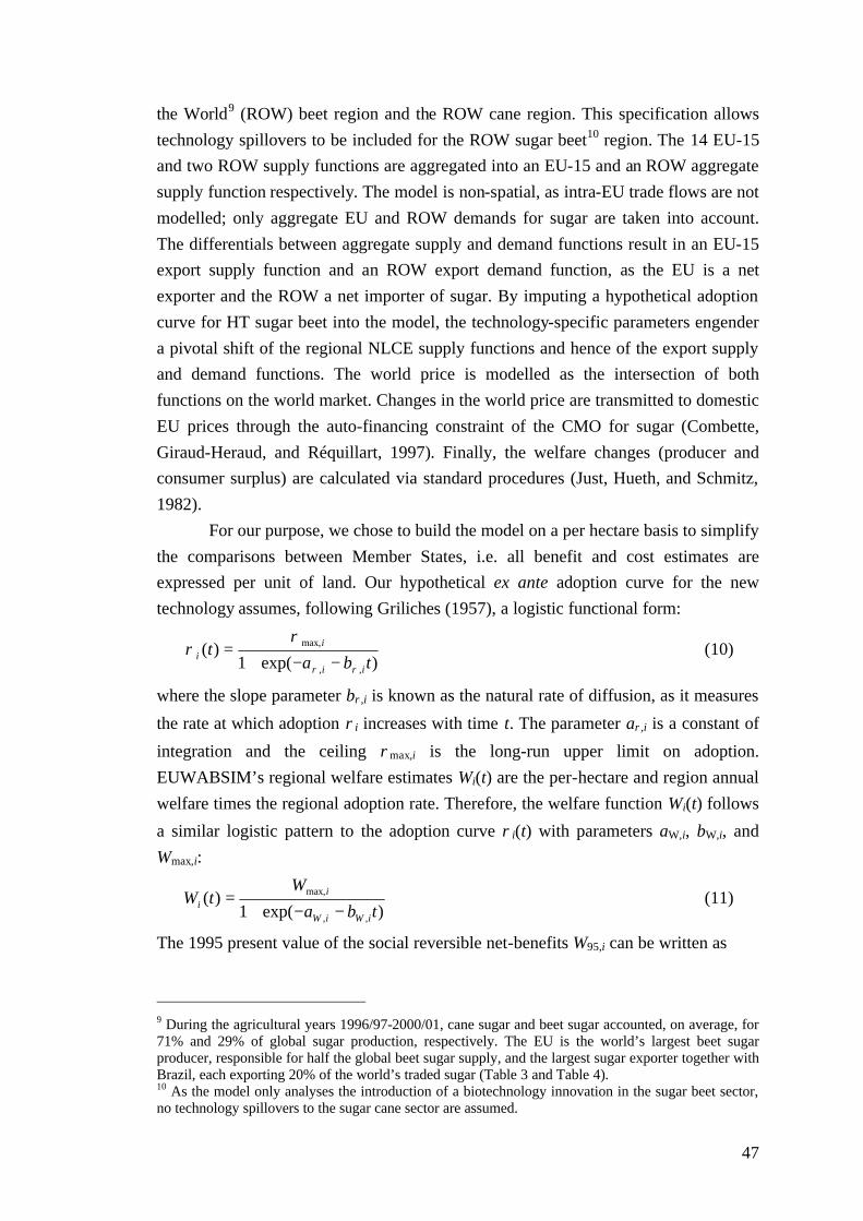
47

the World9 (ROW) beet region and the ROW cane region. This specification allows technology spillovers to be included for the ROW sugar beet10 region. The 14 EU-15 and two ROW supply functions are aggregated into an EU-15 and an ROW aggregate supply function respectively. The model is non-spatial, as intra-EU trade flows are not modelled; only aggregate EU and ROW demands for sugar are taken into account. The differentials between aggregate supply and demand functions result in an EU-15 export supply function and an ROW export demand function, as the EU is a net exporter and the ROW a net importer of sugar. By imputing a hypothetical adoption curve for HT sugar beet into the model, the technology-specific parameters engender a pivotal shift of the regional NLCE supply functions and hence of the export supply and demand functions. The world price is modelled as the intersection of both functions on the world market. Changes in the world price are transmitted to domestic EU prices through the auto-financing constraint of the CMO for sugar (Combette, Giraud-Heraud, and Réquillart, 1997). Finally, the welfare changes (producer and consumer surplus) are calculated via standard procedures (Just, Hueth, and Schmitz, 1982).

For our purpose, we chose to build the model on a per hectare basis to simplify the comparisons between Member States, i.e. all benefit and cost estimates are expressed per unit of land. Our hypothetical ex ante adoption curve for the new technology assumes, following Griliches (1957), a logistic functional form:

)exp(1)(

,,

max,

tbat

ii

ii

ρρ

ρρ

−−+= (10)

where the slope parameter bρ,i is known as the natural rate of diffusion, as it measures

the rate at which adoption ρi increases with time t. The parameter aρ,i is a constant of

integration and the ceiling ρmax,i is the long-run upper limit on adoption. EUWABSIM’s regional welfare estimates Wi(t) are the per-hectare and region annual welfare times the regional adoption rate. Therefore, the welfare function Wi(t) follows

a similar logistic pattern to the adoption curve ρi(t) with parameters aW,i, bW,i, and Wmax,i:

)exp(1)(

,,

max,

tba

WtW

iWiW

ii −−+

= (11)

The 1995 present value of the social reversible net-benefits W95,i can be written as

9 During the agricultural years 1996/97-2000/01, cane sugar and beet sugar accounted, on average, for 71% and 29% of global sugar production, respectively. The EU is the world’s largest beet sugar producer, responsible for half the global beet sugar supply, and the largest sugar exporter together with Brazil, each exporting 20% of the world’s traded sugar (Table 3 and Table 4). 10 As the model only analyses the introduction of a biotechnology innovation in the sugar beet sector, no technology spillovers to the sugar cane sector are assumed.

48

∫∞

−=0

,95 )( dtetWW tii

iµ (12)

with µi the risk-adjusted rate of return derived from the capital asset pricing model (CAPM).11 Thus, all the results we present refer to the year 1995.12 To solve Equation 6, the regional benefits for the EU, WEU(t), calculated on a per hectare basis, are used. As a result of the CMO for sugar, which fixes domestic prices at the beginning of each marketing year, no increases in consumer surplus are found for the EU despite the introduction of HT sugar beet.

Defining the social irreversible benefits R

The irreversible social benefits ri per hectare transgenic sugar beet are approximated by

cDnAr iii ∆+∆= ψω (13)

with ∆Ai is the change in volume of pesticide active ingredients (AI) per unit of land

as a result of the switch from conventional crop protection to HT sugar beet, ω the

average external social cost of pesticide use per unit of active ingredient, ∆ni the change in the number of weeding applications per hectare, D the average diesel use per application and per unit of land, c the average CO2 emission coefficient per unit of

diesel, and ψ the average external social cost per unit CO2 emission. We assume that the per-hectare social irreversible benefits function is proportional to the adoption function:

)exp(1)(

,,

max,

tbartR

ii

iii

ρρ

ρ−−+

= . (14)

The 1995 present value of the social irreversible benefits R95,i can be written as

∫∞

−=0

,95 )( dtetRR tii

iµ . (15)

Data

Because HT sugar beet is not yet adopted, we estimate the adoption parameters of a comparable technology in the USA, i.e. HT Roundup Ready® soybeans (Fernandez-

11 As our model specification includes nontraded assets, the risk-adjusted rate of return derived from the capital asset pricing model was used to calculate the current value of W (McDonald and Siegel, 1986, Abel and Eberley, 1997). The motivation for choosing the risk-adjusted rate of return is that the risk of the additional benefits could be tracked with a dynamic portfolio of market assets:

bmr φσρµ += , where r is the risk-free interest rate, φ the market price of risk, σ the variance

parameter, and ρbm the coefficient of correlation between the asset or portfolio of assets that track W and the whole market portfolio. See Dixit and Pindyck (1994: 147-150) for an elaboration of this assumption. 12 We discuss the stability of the results with respect to time in Section 6.

49

Cornejo and McBride, 2002).13 Therefore, we first transform Equation 10 into its log-linear form:

tbat

tii

ii

i,,

max, )()(

ln ρρρρρ

+=

−. (16)

By assuming a ceiling of ρmax,US = 0.75, the estimated OLS parameters using linear

regression are aρ,US = -2.76, and bρ,US = 0.85. As a benchmark for HT sugar beet in the

EU, we assume a logistic adoption curve with the same ceiling ρmax,i and constant of

integration aρ,i, but with half the speed of US soybean adoption, i.e. bρ,i = 0.43. Assuming the same adoption curve in all EU Member States will allow comparisons to be made between Member States regarding the reversible and irreversible benefits and costs of HT sugar beet.

The social reversible net benefits in the EU consist only of a domestic producer surplus increase.14 As the model is constructed on a per hectare basis, we slightly rewrote EUWABSIM to generate estimates of Wi(t) as the social reversible net benefits per unit of land in region i and year t, by dividing the technology-induced welfare changes by the land allocated to sugar beet, in which adoption of the technology is also endogenous. As a result, EUWABSIM returns estimates for Wi(t) in 14 EU-15 regions and five successive agricultural seasons (t = 1996/97, …, 2000/01). To estimate the parameters aW,i and bW,i of the logistic welfare function (Equation 11), we need an estimate of the ceiling Wmax,i, which we obtain by re-

running EUWABSIM with ρi(t) = ρmax,i = 0.75 and for each year t (t = 1, ..., 5) and taking the maximum of the five estimates. For a given adoption rate, welfare estimates vary from year to year as a result of world price, area, yield and production differences.

For the technology-induced change in volume of pesticide active ingredients,

∆Ai, we use the estimates reported by Coyette et al. (2002) for six European Member States (Belgium, France, Germany, the Netherlands, UK and Spain), covering 72% of total EU sugar beet area. Estimates for the other Member States are obtained by comparing the volume of conventional crop protection (Eurostat, 2000) with that of

HT sugar beet (Bückmann et al., 2000). Regarding the social costs of pesticide use, ω, Pretty et al. (2001) review and adapt three studies on the external costs of agriculture, namely for the UK (Pretty et al., 2000), the USA (Pimentel et al., 1992) and Germany (Waibel and Fleischer, 1998). By aggregating the estimates of (i) the annual human

13 We believe that the US case of HT Roundup Ready® soybeans is comparable with the EU case of HT sugar beet, because of (i) the common embedded technology of herbicide tolerance, (ii) the ubiquitous importance of each crop on both continents, and (iii) the importance of exports of the refined products. 14 As a result of the sugar market policy, consumers do not benefit from productivity increases in sugar beet production.

50

health costs and (ii) loss of biodiversity caused by the application of pesticides in agriculture15, we obtain social costs of €0.87/kg AI for the UK, €0.88/kg AI for the USA and €0.69/kg AI for Germany. For our analysis, we use the third estimate as a conservative proxy for the external costs of pesticide use. The change in the number

of herbicide applications, ∆ni, is calculated by taking the difference in the number of applications for conventional (Schäufele, 2000) and HT sugar beet farming (Bückmann et al., 2000).16 Rasmusson (1998) estimates the average diesel use in sugar beet cultivation, D, at 1.43 litres per herbicide application and per hectare. The average CO2 emission coefficient per unit of diesel is calculated at c = 3.56 kg/l, based on the estimates of Phipps and Park (2002). For the average external social cost

of CO2 emissions we use the estimate of ψ = €77.4/tonne CO2, reported by Pretty et al. (2000).

For estimating the drift rate, α, and the variance rate, σ, of the new ‘herbicide tolerance’ technology, we compute the maximum likelihood estimator assuming continuous growth (Campbell, Lo, and MacKinlay, 1997: Chapter 9.3). We use time-series data on annual gross margin differentials in sugar beet production from 1973 to 1995 as a proxy for estimating the drift and variance rate of future social reversible net benefits. The data are extracted from the EU/SPEL dataset (Eurostat, 1999) for all EU-15 Member States and deflated and converted into real terms using the GDP deflators published by the World Bank (2002). The country-specific hurdle rate is calculated using the estimated drift and variance rate per country and choosing a risk-

free rate of return, r, of 4.5% and a risk-adjusted rate of return, µ, of 10.5% for all

countries. The results for individual countries differ, as the estimated drift rates, iα̂ ,

and variance rates, iσ̂ , vary between EU Member States depending on the time series

for the gross margin per Member State. Finally, data on areas planted to sugar beet, numbers of sugar beet holdings, and currency rates are extracted from the AGRIS dataset (Eurostat, 2003), and household data are reported by the EEA (2001). The

estimated and chosen parameter values are used to calculate β1 in Equation 8, which then was used for the calculation of the hurdle rate in Equation 6.

15 We did not consider the water control costs for pesticides, as the pesticides used with HT and non-HT sugar beet are also used on other crops and the water authorities have to continue testing the water, regardless of the adoption of the new technology. 16 For Belgium, Luxembourg, Denmark, Germany, France, Ireland, Italy, the Netherlands, Austria, Finland, Sweden and the UK, characterised by a herbicide application rate of at least 2.5 applications, the HT system is based on a glyphosate dose of 6 l/ha, sprayed through an average of 2.5 applications (2 x 3 l/ha or 3 x 2 l/ha). For Greece, Spain and Portugal, the average application rate is at most 1.5 applications. In these cases, the counterfactual HT system is assumed to be a one-pass application of 3 l/ha glyphosate.

51

Results and discussion

Table 10 below reports the OLS results of the parameter estimates aW,i and bW,i and the standard errors of the logistic welfare function (EUWABSIM), Wmax,i, the hurdle

rates, and the values of W, R, and I*, presented as annuities (Wa = µW95, Ra = µR95 and

I*a = µI*

95). As expected, the estimates for aW and bW, ranging from -2.98 to -2.75 and 0.37 to 0.44, respectively, are very closely related to the adoption parameters (-2.76 and 0.43, respectively).

The annual social reversible net benefits, Wa, are about €150/ha. Portugal, Finland, Austria, Spain, Belgium and Greece receive highest annual social reversible net benefits per hectare, whereas countries with a larger area allocated to sugar beet have lower average annual social reversible net benefits per hectare. The difference can be explained by the fact that effects on sugar beet produced under the A-quota are larger than effects averaged over A, B and C sugar beet (see Chapter 5). The social irreversible benefits per hectare are small. They range between €1 and €8/ha per Member State, and are on average about €1.6/ha. Table 10: Parameter estimates generated by EUWABSIM, hurdle rates, annual social reversible net-benefits (Wa), social irreversible benefits (Ra) and maximum tolerable social irreversible costs (I*a) per hectare of transgenic sugar beet, per household and per sugar beet growing farmer Member State

aW SE bW SE Wmax (€/ha)

Wa (€/ha)

Ra (€/ha)

Hurdle rate

I*a

(€/ha) I*

a (m€)

I*a

(€/HH) I*

a (€/F)

Belgium -2.85 0.10 0.41 0.03 209 197 2.09 1.26 158 6.7 1.59 436 Denmark -2.78 0.05 0.42 0.02 154 151 2.06 1.73 89 2.4 1.05 306 Germany -2.80 0.08 0.41 0.03 169 164 1.57 1.36 122 25.3 0.68 478 Greece -2.79 0.12 0.37 0.04 213 193 7.97c 3.12 70 1.3 0.36 61 Spain -2.88 0.03 0.44 0.01 210 206 0.53 2.10 99 6.0 0.39 213 France -2.80 0.14 0.40 0.04 139 131 1.05 1.25 106 18.1 0.79 533 Ireland -2.77 0.01 0.42 0.00 155 154 -0.96c 2.29 66 0.9 0.81 215 Italy -2.83 0.09 0.40 0.03 156 146 2.32 1.82 82 9.3 0.42 148 Netherlands -2.80 0.08 0.41 0.02 144 137 0.83 1.31 106 5.1 0.80 265 Austria -2.78 0.06 0.41 0.02 213 207 3.36 2.88 75 1.5 0.46 129 Portugal -2.98 0.17 0.44 0.05 313 294 -0.65c 1.67d 175 0.5 0.13 599 Finland -2.86 0.15 0.39 0.05 270 246 0.74 3.69 67 1.0 0.46 247 Sweden -2.75 0.06 0.40 0.02 143 139 0.18 3.01 46 1.1 0.29 214 UK -2.79 0.12 0.39 0.04 121 113 1.78 1.76 66 4.5 0.21 406 EUa -2.78 0.07 0.41 0.02 158 154 1.59 1.04 149 122.8 0.82 442 EUb -2.78 0.07 0.41 0.02 158 154 1.59 1.67 94 77.1 0.52 277 SE: standard error; HH: household; F: farmer a The hurdle rate is estimated based on the average gross margin for the whole EU. b In this case, the hurdle rate is a sugar beet area-weighted average of the Member States’ estimates. c The extreme estimates for Greece, Ireland and Portugal are probably due to data inconsistencies in the Eurostat (2000) dataset. These countries only cover 4% of total EU area allocated to sugar beet, such that the EU average is almost not affected. d For Portugal, no data on margins have been found. The EU area-weighted average has been used as a proxy for its hurdle rate. The estimated hurdle rates are entirely consistent with expectations. We observe a bimodal distribution. Areas with a comparative advantage in sugar beet production, such as France, Belgium, the Netherlands, Germany, Denmark, the UK and Italy,

52

have low hurdle rates (1.25-1.82), whereas areas with no comparative advantage, such as Spain, Ireland, Austria, Sweden, Greece and Finland, have higher rates (2.10-3.69), requiring higher values of W to justify a release of HT sugar beet. The hurdle rate for the EU using the area-weighted result is about 1.6717. This means that, on average, every Euro of social irreversible net cost has to be matched by about €1.67 of social reversible net benefits to justify release.

The annual maximum tolerable social irreversible costs, I*a, range between €46 and €175 per ha planted to transgenic sugar beet, i.e. in the range of 27-81% of the annual social reversible net benefits. Depending on whether the EU’s hurdle rate is calculated from the aggregate EU gross margins (case EUa in Table 10), or as an area-weighted average of the individual Member States’ hurdle rates (case EUb in Table 10), the estimates for I*a change substantially. In the second case, which is more representative for EU decision-making, maximum tolerable social irreversible costs are €94/ha transgenic sugar beet per year, totalling €77 million per year.

In the last two columns of Table 10, we average the maximum tolerable annual social irreversible costs over all EU households and sugar beet holdings. The maximum tolerable social irreversible costs are below €1 per EU household. If we take loss of biodiversity as the major social irreversible cost, the average willingness to accept the perceived loss of biodiversity per household in the EU should be less than €1 to justify a release of HT sugar beet in the year 1995. This is in line with the observed reluctant attitude of EU citizens regarding transgenic crops and the extent to which this translates into a relatively high willingness to pay to avoid these products (Burton et al., 2001).

If we divide the cost over the ‘responsible’ sugar beet growers, as if the externality remained on the farm, logically much higher values are found. The maximum tolerable irreversible costs per farmer are about €277, ranging from €61 for Greece to €533 for France.

The maximum tolerable social irreversible costs are about 60 times larger than the social irreversible benefits. As both indicators include the same environmental effects, i.e. impact of pesticide use on the environment, biodiversity and climate change, it is unlikely that the unknown true social irreversible costs will be that high. Table 11 below reports the result of a sensitivity analysis using different speeds of adoption and adoption ceilings. The benchmark values are presented in bold. The analysis confirms that our results are very robust. The sensitivity elasticities with

17 The low value for EUa can be explained by the fact that aggregating largely averages out fluctuations, resulting in a lower variance in comparison with the individual Member States. Decisions based upon this hurdle rate have to be interpreted as being made by one decision-maker who decides for the EU as one region (see concluding chapter).

53

respect to adoption speed, i.e. (∂Wa/∂b)(b/Wa) and (∂I*a/∂b)(b/I*

a), are about 0.01. This means that a 100% change of the adoption speed only affects the results by 1%. Table 11: Social reversible net benefits and maximum tolerable social irreversible costs per hectare of transgenic sugar beet for different adoption ceilings and adoption speeds of HT sugar beet in the EU Adoption Adoption ceiling speed Wa (€/ha) I*

a (€/ha) 25% 50% 75% 25% 50% 75% 25% 150.88 150.82 150.77 92.18 92.14 92.11 50% 153.95 153.86 153.77 94.02 93.97 93.92 75% 155.01 154.90 154.79 94.66 94.60 94.53 100% 155.37 155.24 155.12 94.87 94.80 94.73 Finally, the total social reversible benefits forgone if the de facto moratorium is not lifted are of the order of €127 million per year. The total value is very high, but very small on a per household basis. This indicates a general problem with introducing new technologies. The average benefits per household are often very small and this can explain the reluctance of a large segment of society towards new technologies.

Conclusion

In this chapter we addressed the multi-dimensional features of cost-benefit analysis for genetically engineered crops. Whereas most literature on the economic impact of transgenic crops remains entirely focused on the estimation of private reversible net benefits, our study tries to fill a gap in the literature, by assessing the social irreversible benefits and costs of a biotechnology innovation in the sugar industry. Applying a real option approach allows us to estimate the maximum tolerable social irreversible costs, given the social reversible net benefits estimated ex ante using the model developed in Chapter 1 and the social irreversible benefits calculated from secondary data sources.

From the viewpoint of an average EU household, the annual social irreversible costs should not exceed a threshold of roughly €1 if the release of transgenic HT sugar beet in the EU is to be justified. If the average household’s perceived loss of biodiversity caused by HT sugar beet exceeds €1 per year, they would not benefit from the new technology and the de facto moratorium of the EU on transgenic crops for HT sugar beet would be justified.

The benefits forgone for the EU are about €127 million per year. Areas with comparative advantage in sugar beet cultivation (the central EU regions) have low hurdle rates and impose weaker constraints on the maximum tolerable social irreversible costs than less favoured areas (the extreme southerly and northerly EU regions).

54

As GE crops will be released only if considered safe for human consumption, the major regulatory issues concerning their release are issues related to environmental impacts of GE crops (e.g. impacts on biodiversity) and issues of coexistence with non-GE crops (e.g. pollen flow). In the EU, three types of rules and regulations are evolving for governing the coexistence of GE and non-GE crops. The annual social reversible net benefits per hectare provide a first indicator about the maximum costs farmers are willing to bear for complying with regulations. According to our analysis, adopting farmers will not be willing to pay more than about €150/ha to comply with coexistence rules and regulations. As those amounts are relatively small on a per hectare basis to cover additional coexistence costs, adoption will only become economically attractive if farmers can realise economies of scale, lowering coexistence costs per hectare.

The results were calculated based from the perspective of a decision-maker, facing the decision on whether or not to permit the release of HT sugar beet in the year 1995. Since then eleven years have passed. Are the results different today? The EU policy on sugar beets has not significantly changed until 2006 and it is reasonable to expect that incremental benefits have not changed as well. Some small deviations from the values for the hurdle rates presented may occur because of changes in the estimated drift and variance rate adding time series data till the year 2003, but the general results remain the same. This implies that our findings are still valid today. However, these results cannot be used to justify the de facto moratorium in general: our results relate to transgenic sugar beet only, whereas the moratorium covers all transgenic crops. Our proposed methodology offers a tool for EU decision-makers. The latter have to weigh preferences of individual Member States at the EU level. In Chapter 5 we construct and compare different weighing systems for EU decisions based on the real option approach.

The change of the EU sugar regime in 2006 may have an impact on the results (see Chapter 5). It can be expected that the incremental net benefits of HT sugar beet will decrease with a partial liberalisation of the EU sugar market (Frandsen et al., 2003). Research in this direction has been initiated under the EUWAB project (see Chapter 5). Finally, some recent research claims a positive effect of HT sugar beet on biodiversity (Coghlan, 2003). If these claims are confirmed, consumer perceptions about the impact on biodiversity may become positive in the long run.

55

Chapter 3: First impact of biotechnology in the EU: Bt maize adoption in Spain1

Introduction

Since the Second World War, the industrialisation of maize growing in Europe has essentially been driven by technological (genetics, mechanics and chemistry) and economic change. The innovation wave started with the commercialisation of hybrid maize in the fifties (Griliches, 1958). In the seventies, technical and economic constraints emerged due to a slowing down of growth in productivity (Gaillard, 1988). During the eighties, fixed costs increased, causing a sharp decline in maize profitability (Le Stum and Camaret, 1989). Today, the sector faces structural constraints, raising the demand for cost-reducing technological innovations such as biotechnology. In 1998, two transgenic maize varieties from Syngenta Seeds were approved for commercialisation in the EU. However, in 1999 the EU issued a de facto moratorium on new approvals of transgenic crops. In Spain, as a response to the moratorium, Syngenta voluntarily agreed to ‘freeze’ its transgenic seed supply of the variety Compa CB to its 1998 level. Hence, Spain is the first EU country where transgenic crops are grown by farmers on a commercial scale.

The purpose of this chapter is to estimate the first impact of a biotechnology innovation in the EU, i.e. transgenic maize in Spanish agriculture. Moreover, we assess the temporal variability of the impact estimates and the sensitivity of the model to the limited set of data and assumptions.

Economic importance of maize on a world-wide scale

Maize is the world’s most ubiquitous cereal (Table 12). It is cultivated from the equator to roughly 50º north or south latitude, from sea level to more than 3000 m altitude. No other cereal is used in as many different ways; nearly every part of the maize plant has economic value. Moreover, growing incomes in developing countries have stimulated demand for meat and poultry consumption and, as a result, derived demand for maize as animal feed (Pingali, 2001).

The present study concentrates on grain maize. Table 12 shows that, while grain maize is important in all continents, yields vary greatly, ranging from 1.6 t ha-1 in Africa to 10.6 t ha-1 in Belgium. Three subcontinents (USA, South-America and Asia) produce three quarters and export 11% of global maize (Pingali, 2001). The

1 A previous version of this chapter with previous results has been published as: Demont, M., and E. Tollens. “First impact of biotechnology in the EU: Bt maize adoption in Spain.” Annals of Applied Biology 145(2004):197-207.

56

three largest EU maize producers, producing 77% of EU maize output, are France (40%), Italy (26%) and Spain (11%). Table 12: Importance of grain maize growing in the world, average 1998-2003

Area (mha) % Yield (t/ha) Production (mt) % %EU Africa 26.0 18.7% 1.6 42.6 7.0% Asia 43.1 31.0% 3.8 163.8 26.8% Canada 1.2 0.9% 7.3 8.7 1.4% EU-15 4.3 3.1% 8.8 38.1 6.2% 100.0% Austria 0.2 0.1% 9.4 1.7 0.3% 4.5% Belgium-Luxembourg 0.0 0.0% 10.6 0.4 0.1% 1.1% France 1.8 1.3% 8.6 15.2 2.5% 39.8% Germany 0.4 0.3% 8.6 3.3 0.5% 8.8% Greece 0.2 0.2% 9.3 2.0 0.3% 5.3% Italy 1.1 0.8% 9.4 10.1 1.6% 26.4% The Netherlands 0.0 0.0% 8.6 0.2 0.0% 0.5% Portugal 0.2 0.1% 5.8 0.9 0.1% 2.4% Spain 0.5 0.3% 9.5 4.3 0.7% 11.3% South-America 17.2 12.4% 3.4 59.0 9.6% USA 28.7 20.6% 8.5 244.4 40.0% Other 18.6 13.4% 3.0 55.2 9.0% World 139.0 100.0% 4.4 611.7 100.0% Source: FAO (2006)

Table 13: Maize supply balance in Spain, 1998-2001 1998 1999 2000 2001 Average 1998-2001 Production (t) 4,349,070 3,731,000 3,991,752 4,956,600 4,257,106 Import (t) 3,500,000 3,524,000 3,657,000 3,578,000 3,564,750 Export (t) 691,000 535,000 603,000 648,000 619,250 Stocks (t) 1,210,000 800,000 960,000 910,000 970,000 Stock changes (t) 150,000 -410,000 160,000 -50,000 -37,500 Domestic supply (t) 7,008,070 7,130,000 6,885,752 7,936,600 7,240,106 Domestic uses (t) 7,008,000 7,130,000 6,621,000 7,937,000 7,174,000 Animal feed (t) 5,975,000 6,075,000 5,535,000 6,804,000 6,097,250 Industrial use (t) 954,000 975,000 1,000,000 1,050,000 994,750 Human consumption (t) 48,000 47,000 52,000 43,000 47,500 Seed (t) 15,000 19,000 20,000 20,000 18,500 Loss (t) 16,000 14,000 14,000 20,000 16,000 Degree of self-sufficiency (%) 62.1% 52.3% 58.0% 62.5% 58.7% Source: Eurostat (2003)

Economic importance of maize crop protection

The corn borer

The European Corn Borer (ECB) [Ostrinia nubilalis (Hübner)] and the Mediterranean Corn Borer (MCB) [Sesamia nonagrioides (Lefebvre)] are economically important pests. In North-America and Central-Europe, losses are primarily caused by the ECB. At a continental level, the number of ECB generations increases progressively from north to south (Mason et al., 1996). In contrast to the USA Corn Belt, where ECB

57

occurs bivoltine, a single generation is observed in Central-Europe (Bohn et al., 1999), while in southern Europe up to three generations occur (Kergoat, 1999).

The MCB is considered to be one of the most severe maize pests around the Mediterranean Sea and Morocco. Like the ECB, the number of generations increases according to latitude. Two generations prevail, but a single generation also occurs in some areas, like the Azores. In the northeast of Spain, the south of Portugal, Sardinia and Greece, three generations dominate, while four generations can be observed in Morocco (Cordero et al., 1998).

Both insects cause severe crop losses in Spanish maize production. The degree of crop loss largely determines whether the adoption of a pest control strategy is economical. Corn borers cause severe physical damage to the plant. The borer penetrates the stalk and excavates large tunnels that result in important yield losses. This complicates the circulation of water and nutrients to the plant and the ear. The timing of corn borer attack is important and plants are most vulnerable before physical maturity (Jansens et al., 1997).

Crop protection: insecticides, Bt and Bt maize

Larvae from corn borers are difficult to control with chemical insecticides (organophosphates and synthetic pyrethroids) because they are vulnerable to sprays or residues for only a short time before they bore into and are protected by the cob, sheath-collar, or stalk (Jansens et al., 1997). Insecticides are effective when the larvae have just hatched or when they migrate to neighbouring plants (Velasco et al., 1999). Therefore, proper timing of insecticide application is crucial for success and repeated applications are often necessary. However, actual practices are rarely optimal, such that the use of insecticides is limited in Spain (Brookes, 2002).

Bacillus thuringiensis (Bt) is a naturally-occurring soil borne bacterium that is found worldwide. A unique feature of this bacterium is its production of crystal-like (Cry) proteins that selectively kill specific groups of insects (Ostlie, Hutchison, and Hellmich, 1997). Bt incorporated into sprays provides organic farmers with a natural crop protection tool against corn borers.

Plant geneticists create Bt maize by inserting a gene of the bacterium, that causes the plant to produce the toxin. Depending on the gene, the proteins Cry1Ab, Cry1Ac, Cry1B or Cry9C are produced. Labatte et al. (1996) demonstrated that Bt maize has a higher efficacy and shorter time response than insecticides, regardless of the infestation date. Therefore, Bt maize has the potential to dramatically improve the control of corn borer, compared with current practices.

58

Adoption of Bt maize

Transgenic maize was first commercialised in the USA and in Canada in 1996 and two years later in Argentina, South-Africa and Spain. Since then, the adoption has increased up to 15.5 million ha in 2003 (Table 14). The majority of transgenic maize, i.e. 9.1 million ha, are insect resistant (IR) Bt varieties. The other varieties are herbicide tolerant (HT) or stacked IR and HT. The experiences of Bt maize growers all over the world are well recorded, extensively reviewed by James (2003a). Yield gains due to Bt maize are estimated at 5% in the temperate growing areas and 10% in the tropical areas, where there are more and overlapping generations of pests leading to higher infestations and losses. Farmers assign Bt maize high value because it is a convenient and cost effective technology that allows them to manage risk in an uncertain environment and offers insurance2 against devastating crop losses in years when pest infestations are unusually high. Moreover, the technology offers safer feed and food products than conventional maize with lower levels of harmful mycotoxins (James, 2003a). Table 14: Adoption of transgenic and Bt maize in the world and in the EU, 1996-2003 Area 1996 1997 1998 1999 2000 2001 2002 2003 World (mha) Transgenic maize 0.3 3.2 8.3 11.1 10.3 9.8 12.4 15.5 Bt maize 0.3 3.0 6.7 7.5 6.8 5.9 7.7 9.1 EU Bt maize Spain (ha) 0 0 22,000 30,000 20,000 25,000 25,000 32,000 Spain (%) 0 0 4.8% 7.6% 4.6% 5.0% 5.4% 6.8% France (ha) 0 0 2,000 <2,000 <500 0 0 0 Germany (ha) 0 0 0 0 <500 <500 <500 <500 Portugal (ha) 0 0 0 1,000 0 0 0 0 James (1997, 1998, 2000, 2001, 2002, 2003a, 2003b)

On the 26 March 1998, Syngenta’s Bt maize varieties Compa CB (Bt 176) and Jordi CB were registered in the Commercial Variety Register in Spain and approved for commercialisation, but only the first variety has been sold effectively. The main adopting regions were Catalunya (13%), Aragon (11%), Castilla-La Mancha (9%), Madrid (9%), Navarra (4%), Andalusia (3%) and Extremadura (2%) (Alcalde, 2003). Table 14 shows that during 1998-2002 Bt maize adoption in Spain stagnated at about 25 000 ha because of Syngenta’s voluntary arrangement. In 2003 this constraint was lifted and the Ministry of Agriculture approved five new varieties, developed by Syngenta, Pioneer, Monsanto, Nickerson and Limagrain. In the same year, the area planted to Bt maize increased to 32 000 ha (James, 2003a).

2 However, Hurley, Mitchell, and Rice (2004) demonstrate that the insurance argument does not always hold (see Chapter 5).

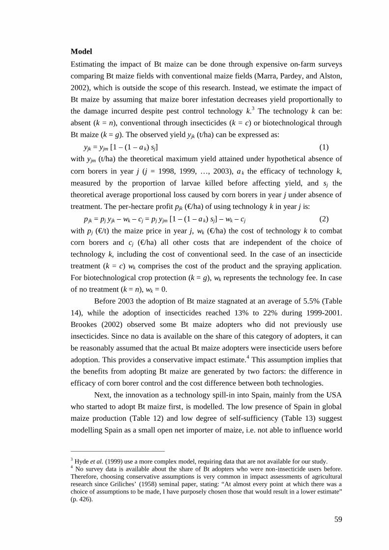
59

Model

Estimating the impact of Bt maize can be done through expensive on-farm surveys comparing Bt maize fields with conventional maize fields (Marra, Pardey, and Alston, 2002), which is outside the scope of this research. Instead, we estimate the impact of Bt maize by assuming that maize borer infestation decreases yield proportionally to the damage incurred despite pest control technology k.3 The technology k can be: absent (k = n), conventional through insecticides (k = c) or biotechnological through Bt maize (k = g). The observed yield yjk (t/ha) can be expressed as:

yjk = yjm [1 – (1 – αk) sj] (1) with yjm (t/ha) the theoretical maximum yield attained under hypothetical absence of

corn borers in year j (j = 1998, 1999, …, 2003), αk the efficacy of technology k, measured by the proportion of larvae killed before affecting yield, and sj the theoretical average proportional loss caused by corn borers in year j under absence of treatment. The per-hectare profit pjk (€/ha) of using technology k in year j is:

πjk = pj yjk – wk – cj = pj yjm [1 – (1 – αk) sj] – wk – cj (2) with pj (€/t) the maize price in year j, wk (€/ha) the cost of technology k to combat corn borers and cj (€/ha) all other costs that are independent of the choice of technology k, including the cost of conventional seed. In the case of an insecticide treatment (k = c) wk comprises the cost of the product and the spraying application. For biotechnological crop protection (k = g), wk represents the technology fee. In case of no treatment (k = n), wk = 0.

Before 2003 the adoption of Bt maize stagnated at an average of 5.5% (Table 14), while the adoption of insecticides reached 13% to 22% during 1999-2001. Brookes (2002) observed some Bt maize adopters who did not previously use insecticides. Since no data is available on the share of this category of adopters, it can be reasonably assumed that the actual Bt maize adopters were insecticide users before adoption. This provides a conservative impact estimate.4 This assumption implies that the benefits from adopting Bt maize are generated by two factors: the difference in efficacy of corn borer control and the cost difference between both technologies.

Next, the innovation as a technology spill-in into Spain, mainly from the USA who started to adopt Bt maize first, is modelled. The low presence of Spain in global maize production (Table 12) and low degree of self-sufficiency (Table 13) suggest modelling Spain as a small open net importer of maize, i.e. not able to influence world

3 Hyde et al. (1999) use a more complex model, requiring data that are not available for our study. 4 No survey data is available about the share of Bt adopters who were non-insecticide users before. Therefore, choosing conservative assumptions is very common in impact assessments of agricultural research since Griliches’ (1958) seminal paper, stating: “At almost every point at which there was a choice of assumptions to be made, I have purposely chosen those that would result in a lower estimate” (p. 426).

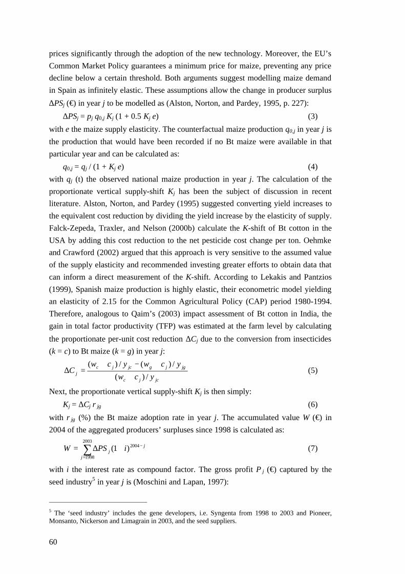
60

prices significantly through the adoption of the new technology. Moreover, the EU’s Common Market Policy guarantees a minimum price for maize, preventing any price decline below a certain threshold. Both arguments suggest modelling maize demand in Spain as infinitely elastic. These assumptions allow the change in producer surplus

∆PSj (€) in year j to be modelled as (Alston, Norton, and Pardey, 1995, p. 227):

∆PSj = pj q0,j Kj (1 + 0.5 Kj ε) (3)

with ε the maize supply elasticity. The counterfactual maize production q0,j in year j is the production that would have been recorded if no Bt maize were available in that particular year and can be calculated as:

q0,j = qj / (1 + Kj ε) (4) with qj (t) the observed national maize production in year j. The calculation of the proportionate vertical supply-shift Kj has been the subject of discussion in recent literature. Alston, Norton, and Pardey (1995) suggested converting yield increases to the equivalent cost reduction by dividing the yield increase by the elasticity of supply. Falck-Zepeda, Traxler, and Nelson (2000b) calculate the K-shift of Bt cotton in the USA by adding this cost reduction to the net pesticide cost change per ton. Oehmke and Crawford (2002) argued that this approach is very sensitive to the assumed value of the supply elasticity and recommended investing greater efforts to obtain data that can inform a direct measurement of the K-shift. According to Lekakis and Pantzios (1999), Spanish maize production is highly elastic, their econometric model yielding an elasticity of 2.15 for the Common Agricultural Policy (CAP) period 1980-1994. Therefore, analogous to Qaim’s (2003) impact assessment of Bt cotton in India, the gain in total factor productivity (TFP) was estimated at the farm level by calculating

the proportionate per-unit cost reduction ∆Cj due to the conversion from insecticides (k = c) to Bt maize (k = g) in year j:

jcjc

jgjgjcjcj ycw

ycwycwC

/)(

/)(/)(

+

+−+=∆ (5)

Next, the proportionate vertical supply-shift Kj is then simply:

Kj = ∆Cj ρjg (6)

with ρjg (%) the Bt maize adoption rate in year j. The accumulated value W (€) in 2004 of the aggregated producers’ surpluses since 1998 is calculated as:

∑=

−+∆=2003

1998

2004)1(j

jj iPSW (7)

with i the interest rate as compound factor. The gross profit Πj (€) captured by the seed industry5 in year j is (Moschini and Lapan, 1997):

5 The ‘seed industry’ includes the gene developers, i.e. Syngenta from 1998 to 2003 and Pioneer, Monsanto, Nickerson and Limagrain in 2003, and the seed suppliers.

61

Πj = wg Lj ρjg (8) with Lj (ha) the total amount of land allocated to maize production. The present value

Π (€) in 2004 of the aggregated gross profits since 1998 is:

∑=

−+Π=Π2003

1998

2004)1(j

jj i (9)

Finally, the accumulated value in 2004 of the total welfare increase Wtot (€) in Spain is:

Wtot = W + Π (10) It is important to note that the ex post welfare calculation only contains private reversible effects. In reality, technologies also engender non-private effects, the so-called externalities (Figure 3). A growing body of scientific literature about the non-private effects of Bt maize is available, reviewed by (James, 2003a). The major concerns include (1) effects on non-target organisms, (2) gene flow, (3) the impact of Cry1Ab proteins in soil and surface water, (4) the evolution of pest resistance, (5) the development of antibiotic resistance and (6) food and feed safety aspects of Bt maize. However, positive externalities are also reported, such as (1) lower contamination of aquifers with insecticides, (2) lower farmers’ exposure to insecticides and (3) lower levels of the mycotoxin fumonisin in Bt maize. Some of these non-private effects are potentially irreversible. For a detailed review on irreversibility, how to include it into welfare analysis and the application of the concept on a concrete case study, see Introduction and Chapter 2.

Data

An important constraint for this impact assessment is the scarcity and low accuracy of data. Therefore, following Davis and Espinoza (1998), stochastic simulation is used through the software @Risk of Palisade Corporation. For uncertain parameters prior stochastic distributions are introduced and through Monte Carlo simulation techniques, distributions for the outcomes in the model are generated.

Insecticide use and cost

During 1999-2001, only 59,000 to 98,000 ha, i.e. 13% to 22% of total maize area was sprayed with insecticides against ECB and MCB (Brookes, 2002). The uncertainty

around insecticide adoption ρc was modelled through a triangular distribution with a minimum of 13%, a most likely value of 18% and a maximum of 22%:

ρjc ~ Triangular(13%; 18%; 22%) (11) This is higher than the reported 5% in the US Corn Belt (Gianessi and Carpenter, 1999), 5% in Italy, 14% in France and 10% in Germany (Gianessi, Sankula, and Reigner, 2003a).

62

Estimates for the insecticide cost for corn borer control are reported by Brookes (2002). Farmers apply one or two insecticide treatments for ECB control. The insecticide cost per hectare wirr (€/ha) in irrigated maize, including the cost of the product and the application, is €18-24/ha. wirr is modelled as:

wirr ~ Triangular(€18/ha; €42/ha; €66/ha) (12) The minimum is based on one treatment at a cost of €18/ha. The maximum is based on two treatments at the maximum cost of €24/ha and including one treatment for control of spider mites6 at a cost of €18/ha. The most likely value is the average of both. The same rationale was applied for aerial spraying (€36-42/ha) and the insecticide cost per hectare wair (€/ha) is modelled as:

wair ~ Triangular(€36/ha; €69/ha; €102/ha) (13) The average insecticide cost per hectare wc (€/ha) for both spraying techniques is

weighted according to the share of irrigated land φ in maize cultivation:

wc = wirr φ + wair (1 – φ) (14)

Technology fee

The technology fee represents the difference between the seed cost of a Bt maize variety and the average seed cost of equivalent conventional varieties. For Syngenta’s Compa CB, Brookes (2002) reported a technology fee of €29-31/ha in Spain. This price is recommended by the seed industry but many farmers pay lower prices through local cooperatives, i.e. €18-19/ha, capturing 70% of the Spanish maize seed market7. These data suggest modelling the technology fee wg (€/ha) as:

wg ~ Triangular(€18/ha; €18/ha; €31/ha) (15)

Theoretical loss due to corn borers

The annual loss due to corn borers varies considerably from year to year. Therefore, a stochastic distribution was constructed for this parameter. For each year j such a distribution was incorporated and assumed to be mutually independent, since Hurley, Mitchell, and Rice (2004) found no statistically8 significant time trends of ECB losses. While gamma as well as lognormal distributions are used to model insect damage, the authors observed a better statistical fitting for the lognormal distribution. Therefore, the proportional loss sj by corn borers in year j in hypothetical absence of pest control is defined as:

sj ~ Lognormal(µ ; σ) (16)

6 In some cases the Bt maize farmer no longer has to spray for spider mites due to the fact that the beneficial insects that control these mites have not been destroyed by the use of insecticides. 7 As a comparison, the technology fee of Bt maize in the USA was estimated at €26/ha in 1997, €22/ha in 1998 and 1999 and €16-17/ha in 2001 (Gianessi et al., 2002), while Benbrook (2001) estimated this fee to be higher, i.e. €25/ha during the same period. 8 with a degree of significance of 5%

63

Data on average annual losses caused by corn borers in Spain are scarce but Alcalde (1999) and Fernández-Anero, Novillo, and Costa (1999) report estimates for these losses sj during the four-year period 1995-1998 (first row in Table 15). The loss is estimated by comparing the yield of Bt varieties with that of isogenic9 varieties. This is the most accurate methodology to estimate the yield boost of transgenic insect resistant varieties (Marra, Pardey, and Alston, 2002). Since only a small sample of four national averages of corn borer damage is disposed of, the median of 0.09 is used

as the most likely value µ for the lognormal distribution. The median is more robust for outliers than the average in the case of such a small skewed sample. The standard

deviation of 0.09 is used as an estimate for σ . Table 15: Data mining of the average theoretical loss by corn borers 1995 1996 1997 1998 Average Median St. Dev. CV (%)e

s Spain 0.09a 0.06a 0.26a 0.09b 0.13 0.09 0.09 74% n Spain 1.49 1.01 4.36 1.49 2.09 1.49 1.53 74% n Cuming County . . . . 1.84c . 1.49 81%c

s Cuming County . . . . 0.11 . 0.09 81% Loss per borer . . . . 0.06d . . . a Alcalde (1999) b Fernández-Anero, Novillo, and Costa (1999) c Hurley, Mitchell, and Rice (2004) d Bohn et al. (1999) e CV represents the coefficient of variation which is the ratio of standard deviation to mean. By dividing the annual loss sj by an average loss of 6% per corn borer per plant (Bohn et al., 1999), estimates of the population sizes are obtained, measured as the average number of borers n per plant (second row in Table 15). In the absence of pest control, on average two corn borers per Spanish maize plant can be found. Calculating the coefficient of variation (last column) allows a comparison of the parameters of the stochastic distribution of Spain with data from the USA. The Spanish situation is most comparable with data from Cuming County (Hurley, Mitchell, and Rice, 2004). The average is high, justifying the use of the median as the most likely value. The coefficient of variation is in the range of values (0.75-1) found in the USA. The occurrence of one severe loss every 4-8 years has also been observed in the USA (Rice and Ostlie, 1997). Finally, since no negative losses or losses greater than 100% can be incurred, the lognormal distribution is truncated to the interval [0,1].

Efficacy of both technologies

Estimates of the efficacy of insecticides to control corn borers vary considerably. Ostlie, Hutchison, and Hellmich (1997) report an efficacy of 80% against first

9 Varieties that have exactly the same genetic composition with the exception of the Bt gene.

64

generation borers and 67% against second generation. Labatte et al. (1996) observe an average efficacy of 72% in case of suboptimal timing. Since timing plays a crucial

role, a wide variation for the insecticide spraying efficacy αc is assumed:

αc ~ Triangular(70%; 80%; 90%) (17) Low values capture the potential impact of the development of ECB resistance against insecticides while high values capture the emergence of technological innovations in conventional spraying techniques.

Regarding the efficacy of Bt maize in Spain, no data is available. The farmers report no yield loss from using it (Brookes, 2002). Labatte et al. (1996) also observe no yield losses in France. We conservatively use the value of 95%. Uncertainty about

the efficacy of Bt maize in Spain αg is modelled by assuming:

αg ~ Triangular(90%; 95%; 100%) (18) Low values capture the potential development of ECB resistance against the Bt toxin.

The efficacy of the absence of a treatment is zero, i.e. αo = 0%. Total average efficacy

αj of the observed mix of technologies in year j in Spain is weighted as follows:

αj = αc ρjc + αg ρjg + αo (1 – ρjc – ρjg) = αc ρjc + αg ρjg (19) The theoretical maximum yield yjm (t/ha) in Equation 1 can now be estimated as:

yjm = yj / [1 – (1 – αj) sj] (20) with yj (t/ha) the observed average national yield.

All other costs

In order to obtain an estimate for cj (€/ha), i.e. all other costs that are independent of the choice of technology k, an estimate for the average maize production costs ACj (€/ha) in Spain is required. Cost estimates from 2001-2003 extracted from the European Commission’s (2006b) Farm Accountancy Data Network (FADN) are used. These gross production cost estimates GCj do not include family labour costs nor interest costs for own capital. Therefore, they consist of a lower estimate for the average maize production costs. As an upper estimate, the per-hectare value of production is used. The most likely value is the average of both limits, i.e.:

ACj ~ Triangular(GCj; (GCj + pj yj)/2, pj yj) (21) An estimate for cj (€/ha) is reconstructed by taking into account national adoption rates and costs of insecticides, Bt maize and the absence of a treatment:

cj = ACj – wc ρjc – wg ρjg – 0.(1 – ρjc – ρjg) (22)

65

Other parameters

Adoption rates (James, 1997, 1998, 2000, 2001, 2002, 2003a, 2003b), yields, area harvested, prices (Eurostat, 2003) and the share of irrigated land in maize cultivation10 (MAPA, 2003, 2004) are modelled as deterministic parameters, i.e. without assuming a stochastic distribution. A maize supply elasticity of 2.15 reported by Lekakis and Pantzios (1999) for the CAP period 1980-1994 is used. Since the authors did not report any standard errors, we construct a non-negative (from economic theory) symmetric triangular distribution for this structural parameter with a minimum of 0, a most likely value of 2.15 and a maximum of twice the base value. All prices and costs are deflated using the GDP deflator (Eurostat, 2003, OECD, 2003b). For the interest rate i a risk-adjusted rate of return of 10.5% derived from the capital asset pricing model (CAPM) is used.

Results

Average impact results

In Table 16 the average values generated by the model are presented. In the eighth column the six-year average (1998-2003) is reported. Annually, Spanish Bt maize adopters gain €1.2 million or €48/ha, taking into account an average loss by corn borers of 9% (Fernández-Anero, Novillo, and Costa, 1999, Alcalde, 1999). The aggregated producer surplus accumulated during the six-year period and actualised to 2004 is €11 million (last column). During the same period, the seed industry extracts an annual gross profit of €0.6 million or an aggregated profit of €5 million from the new technology.11 Average total annual welfare change is €1.8 million and accumulates to €16 million after six years of adoption. Farmers gain two thirds (67%) of the total benefits, while one third (33%) accrues to the seed industry. This benefit sharing is consistent with the majority of biotechnology impact distribution studies in literature (Table 1).

Uncertainty

To obtain detailed information regarding the uncertainty surrounding the average impact results, a distribution is generated for the latter, given the assumed prior distributions for the uncertain parameters. Using the software @Risk from Palisade Corporation a Monte Carlo simulation is conducted and generated 100,000 iterations.

10 The Spanish climate necessitates irrigation. Some 92% of total maize area is irrigated (MAPA, 2003, MAPA, 2004). Only in the north can maize be grown without irrigation. Irrigated land is cultivated more intensively and plant density, investment per unit of land and yields are higher. 11 This gain is distributed among the gene developers and the seed companies that pay a technology license to the former. Since we do not have any information about this contract, we cannot calculate the share captured by the seed companies.

66

The results are presented in Table 17. Total profit for Spanish agriculture lies within a 95% probability interval of €10 million and €23 million (Figure 8), while the seed industry’s gross profit varies from €4 million to €7 million. Thus, with a probability of 95% agriculture captures between 42% and 79% of total profit and the seed industry between 21% and 58%. The idea of agriculture losing money on average by adopting Bt maize is very unlikely and only occurs in 0.002% of iterations. In 93% of the cases, more than half of total benefits accrues to farmers. Table 16: Economic impact of Bt maize on Spanish agriculture and the seed industry, 1998-2003 Year

1998

1999

2000

2001

2002

2003 Average

1998-2003 Aggregated value 2004

Adoption (%) 4.8% 7.6% 4.6% 5.0% 5.4% 6.8% 5.7% 5.7% Bt maize adopters (€/ha) 50.5 50.6 47.9 46.8 45.1 45.7 47.8 415.5 Agriculture (m€) 1.1 1.5 1.0 1.2 1.1 1.5 1.2 10.5 Seed industry (m€) 0.5 0.7 0.5 0.6 0.6 0.8 0.6 5.2 Total impact (m€) 1.6 2.2 1.4 1.8 1.7 2.2 1.8 15.8 Agriculture share (%) 67.9% 67.9% 66.7% 66.2% 65.3% 65.6% 66.6% 66.8% Seed industry share (%) 32.1% 32.1% 33.3% 33.8% 34.7% 34.4% 33.4% 33.2% Table 17: Descriptive statistics of the distribution of the aggregated impact of Bt maize on Spanish agriculture and the seed industry, 1998-2003 Minimum 2.5% probability limit Mean 97.5% probability limit Maximum Agriculture (m€) -0.1 4.2 10.5 17.9 40.4 Seed industry (m€) 4.2 4.3 5.2 6.8 7.3 Total (m€) 6.4 9.7 15.8 23.0 45.9 Agriculture share (%) -1.4% 41.8% 65.1% 79.1% 88.5% Seed industry share (%) 11.5% 20.9% 34.9% 58.3% 101.4%

Va

lue

s in

10

^ -7

Values in Millions

0.000

0.200

0.400

0.600

0.800

1.000

1.200

0 5 10 15 20 25

1818

0 5 10 15 20 25

2.5% 95% 2.5%< > 4.1848 17.9353

Figure 8: Distribution of the aggregated impact of Bt maize on Spanish agriculture (in million €)

67

Sensitivity analysis

Since the model is fed by some uncertain parameters, defined by subjective distributions, it is important to assess the influence of the assumptions on the model results. Therefore, the data generated by the iterations in @Risk are analysed. Normalised regression coefficients in Table 18 reflect the robustness of the model to individual parameter values (see Chapter 1). The coefficient of determination R2 is satisfactorily high in all regressions, signifying that the linear approximation sufficiently explains the variation in the iterations. Table 18: Normalised regression coefficients of the impact of Bt maize in Spain in 2003 Parameter Agriculture Seed industry Total Agriculture (%) Seed industry (%) Theoretical loss s2003 0.778 0.000 0.790 0.519 -0.519 Irrigated insecticide cost wirr 0.490 0.000 0.497 0.572 -0.572 Efficacy insecticides αc -0.215 0.000 -0.218 -0.184 0.184 Technology fee wg -0.167 1.000 -0.025 -0.452 0.452 Efficacy Bt maize αg 0.104 0.000 0.105 0.090 -0.090 Average production cost ACj -0.105 0.000 -0.107 -0.101 0.101 Aerial insecticide cost wair 0.048 0.000 0.049 0.057 -0.057 Adoption of insecticides ρc 0.002 0.000 0.002 0.000 0.000 Supply elasticity -0.004 0.000 -0.004 -0.002 0.002 R2 0.943 1.000 0.941 0.858 0.858 Table 18 illustrates these coefficients for the most recent year, i.e. 2003, the sensitivity estimates for the other years (1998-2002) being essentially the same. In a given year, the theoretical loss by corn borers is the main factor (coefficient of 0.778) explaining the benefits of Bt maize. Temporal and geographic heterogeneity of corn borer infestations significantly influence the payoff of this technology, limiting the input industry’s monopolistic pricing behaviour and farmers’ adoption of the new technology. In some regions and some years, the benefits of the technology simply do not compensate for the high technology fee. Because of this, Spain’s Bt maize adoption potential is limited to 36% (Brookes, 2002). The cost of the conventional technology turns out to be the second most important factor (coefficient of 0.490), due to the wide assumed distribution. Insecticide prices are expected to fall as a reaction on the adoption of Bt maize. As a result, these competition effects will erode the comparative advantage of the new technology. In the third place comes the efficacy of the conventional technology, which is negatively correlated with the impact results (coefficient of -0.215). Any technological innovation able to increase the insecticide efficacy, e.g. a new insecticide or a new managerial spraying or scouting technique, will compete with Bt maize. Finally, the narrow distribution of assumed technology fees has a relatively small negative impact (coefficient of -0.167) on the model outcomes.

68

Due to the static character of the model through Equation 8, the benefits for the seed industry are simply a function of the technology fee. The question is how this price will evolve now that other companies have recently entered the market for transgenic maize seed. Remarkably total benefits (column 4) are hardly affected by the technology fee, although benefit sharing is (columns 5 and 6). Four factors, i.e. the theoretical loss by corn borers (coefficient of 0.519), the cost (coefficient of 0.572) and efficacy (coefficient of -0.184) of the conventional technology and the license between the biotechnology industry and the farmer (coefficient of -0.452) essentially drive the welfare distribution of the new technology.

Discussion

Since plantings of transgenic seed have been limited to a small fraction of the Spanish maize area, i.e. 5.7% on average during 1998-2003, and an even smaller fraction of total Spanish maize supply, i.e. 3.2% on average during 1998-2001 (Eurostat, 2003), the supply shift engendered by the new technology has been small so far. An average vertical and horizontal supply shift of K = 0.18%, respectively J = eK = 0.39% per year during 1998-2003 was found. This supply shift is expected to increase now that Syngenta’s voluntary agreement is lifted and Bt maize adoption is no longer constrained. The limited adoption so far is assumed to be primarily driven by insecticide users switching to Bt maize in search for a more efficient pest control tool. A rational farmer facing economically important ECB losses to the point that Bt maize pays, would also likely adopt insecticides. Because of this assumption, the welfare estimates are conservatively biased downwards. As soon as Bt maize adoption levels increase beyond insecticide adoption levels, an important proportion of the adopters will consist of non-insecticide adopters.

Domestic maize demand is modelled as infinitely elastic in a small open economy. As a result, no price decline is generated by the model and no benefits accrue to Spanish consumers. Spanish maize production is highly elastic, meaning that if the maize sector faced a less elastic downward sloping domestic demand curve, the technology-induced supply-shift would quickly erode domestic prices. Any cost reduction translates in a 2.15-fold production response. Since the EU guarantees a minimum price for maize, Spanish maize farmers are largely protected against price declines and the main resulting effect is a sharp production boost. The latter yields an opportunity to increase the low degree of self-sufficiency of Spanish maize production, i.e. 59% on average during 1998-2001 (Table 13). The lion’s share of Spanish maize supply, i.e. 85% on average, is used by the animal feed industry. Even in case price declines occurred, in the short run benefits would flow to the animal feed industry, cattle farmers, processors and distribution sectors and in the long run to consumers through lower animal product prices.

69

Conclusion

Maize is the most wide-spread cereal on earth and has a wide range of yields. Spain provides 11% of the EU-15’s grain maize. Two types of corn borers cause severe losses in this sector. This opens up perspectives for transgenic Bt maize, providing a tool to control these insects more efficiently. Up to 2002, Syngenta voluntarily limited transgenic maize seed supply to an equivalent of 25,000 ha of the variety Compa CB. As a result, adoption rates stagnated to an average of 5.5% of Spanish maize area.

Conservatively assuming that this minority of Bt maize adopters previously used insecticides, the innovation for a small open net importer of maize is modelled. As a result, during the six-year period 1998-2003 Spanish maize growers capture €10.3 million while the seed industry gains €5.2 million. Two thirds of the benefits accrue to agriculture, while one third is extracted by the industry. This result is primarily sensitive to our assumptions about corn borer losses and insecticide costs.

Up to now, the Spanish situation has been artificial in a sense, since Syngenta voluntarily limited the supply of seed. The question remains as to what extent the observed technology fee was also artificial. The price premium of the seed was similar to the price in the USA. Due to the end of the voluntary agreement in 2003, five new varieties have been approved. With this additional competition in mind it is likely that technology fees will fall. This has happened in all other countries where transgenic crops have been introduced (Gianessi et al., 2002). It is unlikely that the biotechnology industry will be able to extract the lion’s share of the benefits. Literature shows that farmers are generally the main beneficiaries of agricultural biotechnology innovations (Table 1). In the long run, these benefits flow from farmers to downstream sectors, distribution and finally to the consumer.

70

71

Chapter 4: Alston, Norton, and Pardey revisited: Modelling supply shift in equilibrium displacement models

Introduction

In the literature on equilibrium displacement models (EDMs) for returns to research estimations, the Alston, Norton, and Pardey (1995) (ANP) formulation is without doubt the most cited and commonly accepted method. However, Oehmke and Crawford (2002) recently emphasised that “[…] the Alston, Norton, and Pardey calculation of the size of the supply shift, K, introduces a new use of the supply

elasticity, ε, at a particularly crucial point in the calculations” (p. 367), making returns to research estimations much more sensitive to values of the assumed supply elasticity. Recently, Moschini, Lapan, and Sobolevsky (MLS) (2000) proposed a different method, that does not explicitly rely on the widely accepted ANP formulation. Finally, change in revenue (CIR) methods can be widely found that do not explicitly make use of an EDM.

Since some of these different methods are used interchangeably, there is a need for juxtaposing them in an analytical framework. Price et al. (2003) compare the welfare estimates generated by the ANP and MLS methods: “To do this, assumptions concerning supply and demand elasticities and farm-level effects were equalized across the two frameworks” (p. 40). While this reconciliation highlights some interesting differences, their framework is not empirically tractable enough to explain how the differences are generated. Frisvold, Sullivan, and Raneses (2003) algebraically relate and empirically compare the CIR and the ANP method. However, none of these studies have attempted to compare the robustness of these models to the typical stochastic nature of real farm and market level data that are used to run the models.

Therefore, the purpose of this chapter is to fill two gaps in literature. First, we algebraically harmonise and juxtapose five different EDMs commonly used in the economic impact literature of GE crops. Secondly, we follow and extend the recommendations of Davis and Espinoza (1998, 2000), Griffiths and Zhao (2000) and Zhao et al. (2000) and use stochastic sensitivity analysis as a basis for comparison of the different approaches. We define the ‘performance’ of the model as its overall robustness and its robustness to the stochastic nature of its parameters.

Shortly after the publication of ANP’s manuscript, Beattie (1995) wrote: “Science under scarcity seems likely to become an invaluable reference source, not only for economic analysts charged with “carrying out and interpreting research evaluation or priority-setting analyses for administrators,” but for all economists

72

(agricultural and resource economists in particular) with interests in production economics, supply analysis, welfare measurement, and policy analysis generally” (p. 1064). However, in the remainder of the review, Beattie (1995) raised some concerns on the argumentation of ANP regarding the nature of the supply shift in EDMs: “If total benefits from a research-induced supply shift are halved when that shift is deemed to be pivotal rather than parallel, and if producer benefits disappear when the supply shift is pivotal against an inelastic demand, then it seems to me that we have a rather big problem here” (p. 1065). According to ANP, the answer lies in the arguments of Rose (1980): “For most innovations, the best information available may be a cost-reduction estimate for a single point on the supply curve… [It] is unlikely that any knowledge of the shape of the supply curve, or the position at which the single estimate applies, will be available. The only realistic strategy is to assume that the supply shift is parallel” (p. 837).

While the previous discussion concentrates on the nature of the supply shift, in this chapter we would like to draw the attention to the size of the supply shift in EDMs. Alston, Norton, and Pardey (1995) distinguish between the vertical and horizontal displacement of the supply curve: “The relative increase in experimental yield, Y, will translate into an equal, proportional, rightwards shift of industry supply in the quantity direction (i.e., dY/Y = E(Y) = J) under a neutral technical change with fixed factor proportions. To translate this into a measure of K (the percentage shift down of supply in the price direction), we divide by the elasticity of supply: i.e., K =

J/ε = E(Y)/ε ” (p. 339). Falck-Zepeda, Traxler, and Nelson (2000a) follow the ANP approach and observe that when using a low supply elasticity of 0.22 instead of 0.92, US farmer surplus increases by a factor of six. The authors conclude: “Because we do not have strong priors about the validity of either elasticity assumption, we cannot choose one scenario over the other” (p. 31). Indeed, in the remainder of ANP’s manuscript, the authors admit that their formulation makes the calculation of K

extremely sensitive to the value of the supply elasticity: “[…] the supply elasticity, ε, is not bounded between 0 and 1 and errors in its estimation could have relatively

important quantitative implications. Thus, we have advocated using ε = 1 for this step so that K = J ” (p. 361). Oehmke and Crawford (2002) argue against ANP’s suggestion that the supply elasticity be artificially set to one in calculating the supply shift, on both conceptual

and practical grounds: “There are two problems with setting ε = 1 just for the

calculation of K. First it is internally consistent to use one value of ε at one step in a calculation and another value at another step. Second, it negates the conceptual and practical advantages of distinguishing between horizontal and vertical measures of the size of the supply shift” (p. 368). The authors illustrate the shortcomings of the ANP

73

approach through a numerical and empirical example and conclude that “if the researcher does not know the supply elasticity, then the researcher may not be able to evaluate whether the project’s ROR [rate of return] is satisfactory” (p. 368). Instead, in their concluding paragraph, the authors recommend “to invest greater efforts to obtain sound empirical estimates of the supply elasticity” or “to obtain data that can inform a direct measurement of the vertical supply shift, such as accurate enterprise budgets or data sets sufficient to estimate cost functions” (p. 369). Qaim (2003) draws upon the latter recommendation and uses enterprise budgets to estimate the difference in per-unit cost of production due to the adoption of Bt cotton in India. This measure is then “interpreted as the technology’s gain in TFP [total factor productivity] at the farm level” (p. 2123), and provides a direct estimate of the K-shift.

Moschini, Lapan, and Sobolevsky (2000) and Sobolevsky, Moschini, and Lapan (2005) develop a non-linear constant-elasticity (NLCE) EDM to estimate the welfare effects of herbicide tolerant soybeans in the United States of America (USA). Instead of relying on the ANP approach, their methodology features two innovations. First, they endogenise the supply shift into the supply function. Secondly, their EDM assesses research benefits in the market for land supplied to the industry of the crop under research1, instead of the commodity market. Finally, other ad hoc methods can be found that do not explicitly define an EDM. These farm level analyses typically rely on the comparison of farm level gross margins between adopters and non-adopters of the new technology. The difference in gross margins is then aggregated to the entire adopted area through simple homothetic extrapolation.

We run the models using data from the impact study of Bt maize in Spain in Chapter 3. Spain can be considered a small open net importer of maize, facing an infinitely elastic demand. This allows us to isolate the effect of the size of the supply shift on both producer welfare and supply response on one hand from the market effects on the other hand. We model uncertainty through subjective prior distributions and compare the mean and variance of the generated distributions for farmers’ surplus and supply response.

Modelling welfare effects

Our main focus is on the modelling and parameterisation of the supply shift in EDMs due to the adoption of a new research-induced technology. When presented in a standard market model, we graphically distinguish two components of the supply shift

due to a technological innovation. The difference in effective yields ∆Y = yn – yc acts as a horizontal shifter, where yn and yc are the yield obtained with the new versus the

conventional technology, while the per-hectare cost reduction ∆C = cc – cn acts as a

1 In the remainder of the chapter, we will refer to this market as the ‘land market’.

74

vertical shifter, where cc and cn are the average production costs under the conventional versus the new technology,. The proportionate yield boost and per-

hectare cost reduction are calculated as β = ∆Y/yc ∈ [0,1] and γ = ∆C/cc ∈ [0,1].

Change in revenue method (CIR)

If we define p as the price of the crop, L as the total area planted with the crop and ρ

∈ [0,1] as the adoption rate of the new technology, the change in returns to land, labour and management of the farmer due to the adoption of a new technology can be algebraically presented as:

∆RCIR = p∆Y + ∆C (1) This equation states that the change in returns to land is equal to the change in revenues, price time yield increase, less the change in costs. The change in producer surplus and proportionate production increase are:

∆PSCIR = ∆RCIRLρ (2)

JCIR = βρ (3) The change in producer surplus is the returns to land multiplied by the total acreage of the crop time the adoption rate. The proportionate production increase is the proportionate yield boost time the adoption rate.

Alston, Norton, and Pardey (1995)

In literature, three different methods of estimating the supply shift K can be found. First, the standard ANP formulation suggests converting (horizontal) yield increases to the equivalent (vertical) cost reduction by dividing the yield increase by the elasticity of supply, i.e. KANP in equation 4 (Alston, Norton, and Pardey, 1995, p. 360). However, admitting that the suggested formulation is sensitive to supply

elasticity estimates, in the remainder of their manuscript ANP advocate using ε = 1 for the calculation of the supply shift, i.e. KANP1 in equation 5 (Alston, Norton, and Pardey, 1995, p. 361). Finally, following the recommendations of Oehmke and Crawford (2002, p. 369), Qaim (2003, p. 2124) approximates the supply shift by the gain in TFP at the farm level, estimated through the proportionate per-unit cost reduction, i.e. KOCQ in equation 6.

ρεβ

βγ

+

+=

1ANPK (4)

ρββ

γ

+

+=

1ANP1K (5)

75

ρββγ

ρβγ

++

=

+−

−=

1)1()1(

OCQ

c

c

c

c

c

c

ycyc

yc

K (6)

These equations state that the ANP supply shift is a function of the proportionate cost reduction, the yield boost and the supply elastiticy, while the ANP1 and OCQ supply shifts are only a function of the proportionate cost reduction and yield boost.

Next, the change in producer surplus and the supply response for a technology spill-in into a small open economy are calculated as (Alston, Norton, and Pardey, 1995, p. 227):

∆PSj = p q0 Kj (1 + 0.5 Kj ε) (7)

Jj = Kj ε (8)

with q the observed national production, ε the supply elasticity, j ∈ (ANP, ANP1, OCQ) the type of supply shift, q0,j = q/(1+Jj) the counterfactual production, i.e. the production that would have been recorded if the new technology were not available. The change in producer surplus is a function of price, pre-innovation quantity, supply shift and supply elasticity. The supply response or horizontal supply shift equals the vertical supply shift time the supply elasticity.

Moschini, Lapan, and Sobolevsky (2000) (MLS)

Moschini, Lapan, and Sobolevsky (2000) and Sobolevsky, Moschini, and Lapan (2005) develop a NLCE supply curve, adapted to the actual working of the herbicide tolerance trait in the case of transgenic soybeans. Here, we adapt their formulation to make it compatible with the other models. The average land rent function allows yields to respond to prices:

CpG

ApR ∆++

++= + ρ

ηρβ

ρ η1

1)1(

),( (9)

such that the optimal yield function is y(p,ρ) = (1 + ρβ)Gpη with η the elasticity of yield with respect to prices, G and A scale parameters subsuming all other input prices, presumed constant, and calibrated so as to retrieve yield, profit (p = py – c with c the observed national average production costs) and production data for the analysed agricultural season. The average returns to land are a function of the yield boost, the adoption rate, the cost reduction, the price and the yield elasticity. The average supply function is obtained by multiplying the average land supply function by the optimal yield function:

[ ] ηθ ρβρλρρρ GppRpyRLpq )1(),(),(),(),( +== (10)

with λ a scale parameter and θ the elasticity of land supply with respect to profit per

hectare, calibrated as θ = rψ where ψ is elasticity of land supply with respect to maize

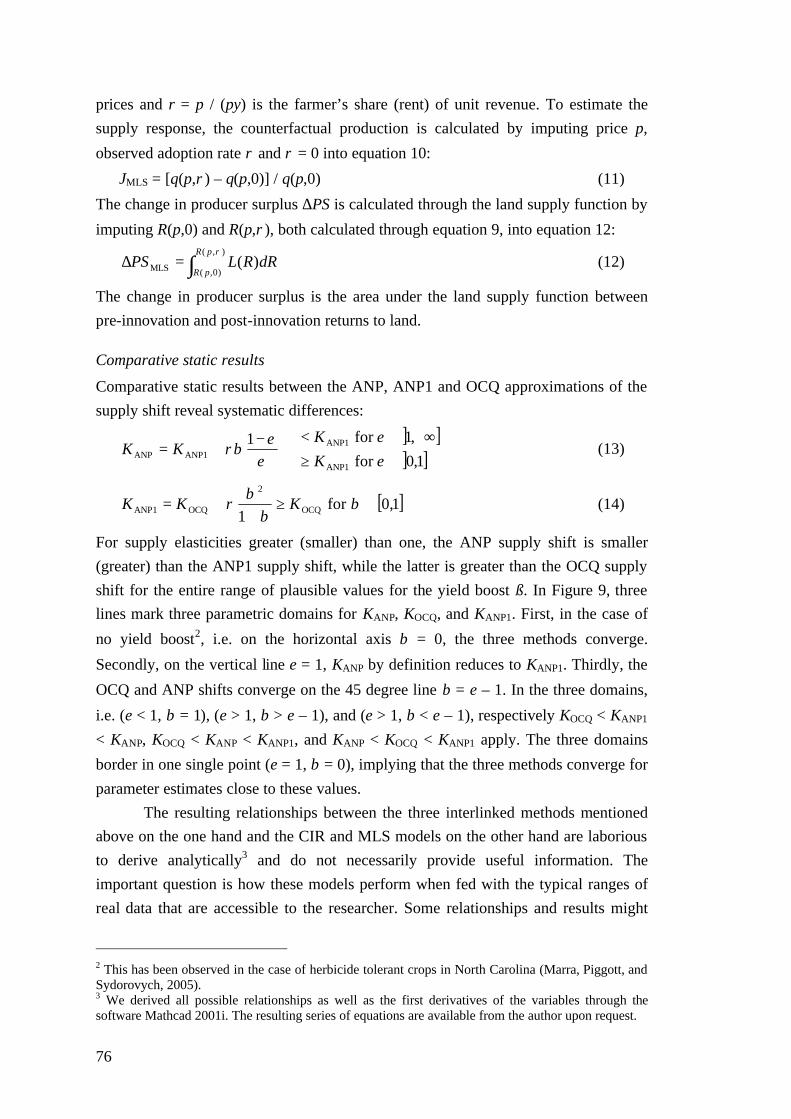
76

prices and r = p / (py) is the farmer’s share (rent) of unit revenue. To estimate the supply response, the counterfactual production is calculated by imputing price p,

observed adoption rate ρ and ρ = 0 into equation 10:

JMLS = [q(p,ρ) – q(p,0)] / q(p,0) (11)

The change in producer surplus ∆PS is calculated through the land supply function by

imputing R(p,0) and R(p,ρ), both calculated through equation 9, into equation 12:

∫=∆),(

)0,(MLS )(ρpR

pRdRRLPS (12)

The change in producer surplus is the area under the land supply function between pre-innovation and post-innovation returns to land.

Comparative static results

Comparative static results between the ANP, ANP1 and OCQ approximations of the supply shift reveal systematic differences:

] ]] ]

∈≥+∞∈<−

+=1,0for

,1for1

1ANP

1ANP1ANPANP ε

εε

ερβ

K

KKK (13)

[ ]1,0for1 OCQ

2

OCQ1ANP ∈≥+

+= ββ

βρ KKK (14)

For supply elasticities greater (smaller) than one, the ANP supply shift is smaller (greater) than the ANP1 supply shift, while the latter is greater than the OCQ supply shift for the entire range of plausible values for the yield boost ß. In Figure 9, three lines mark three parametric domains for KANP, KOCQ, and KANP1. First, in the case of

no yield boost2, i.e. on the horizontal axis β = 0, the three methods converge.

Secondly, on the vertical line ε = 1, KANP by definition reduces to KANP1. Thirdly, the

OCQ and ANP shifts converge on the 45 degree line β = ε – 1. In the three domains,

i.e. (ε < 1, β = 1), (ε > 1, β > ε – 1), and (ε > 1, β < ε – 1), respectively KOCQ < KANP1 < KANP, KOCQ < KANP < KANP1, and KANP < KOCQ < KANP1 apply. The three domains

border in one single point (ε = 1, β = 0), implying that the three methods converge for parameter estimates close to these values.

The resulting relationships between the three interlinked methods mentioned above on the one hand and the CIR and MLS models on the other hand are laborious to derive analytically3 and do not necessarily provide useful information. The important question is how these models perform when fed with the typical ranges of real data that are accessible to the researcher. Some relationships and results might

2 This has been observed in the case of herbicide tolerant crops in North Carolina (Marra, Piggott, and Sydorovych, 2005). 3 We derived all possible relationships as well as the first derivatives of the variables through the software Mathcad 2001i. The resulting series of equations are available from the author upon request.

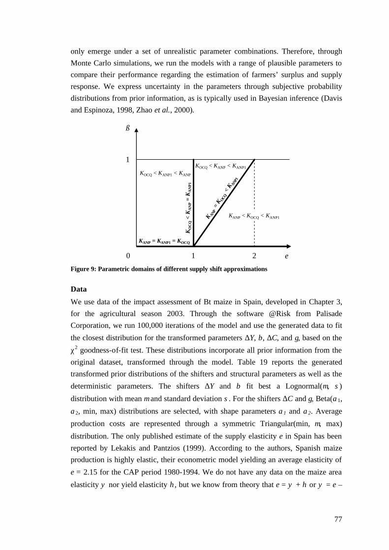
77

only emerge under a set of unrealistic parameter combinations. Therefore, through Monte Carlo simulations, we run the models with a range of plausible parameters to compare their performance regarding the estimation of farmers’ surplus and supply response. We express uncertainty in the parameters through subjective probability distributions from prior information, as is typically used in Bayesian inference (Davis and Espinoza, 1998, Zhao et al., 2000).

ß

ε21

1

0

KOCQ < KANP1 < KANP

KO

CQ

< K

AN

P=

KA

NP1

KANP = KANP1 = KOCQ

K ANP

= K OCQ

< K AN

P1

KOCQ < KANP < KANP1

KANP < KOCQ < KANP1

Figure 9: Parametric domains of different supply shift approximations

Data

We use data of the impact assessment of Bt maize in Spain, developed in Chapter 3, for the agricultural season 2003. Through the software @Risk from Palisade Corporation, we run 100,000 iterations of the model and use the generated data to fit

the closest distribution for the transformed parameters ∆Y, β, ∆C, and γ, based on the

χ2 goodness-of-fit test. These distributions incorporate all prior information from the original dataset, transformed through the model. Table 19 reports the generated transformed prior distributions of the shifters and structural parameters as well as the

deterministic parameters. The shifters ∆Y and β fit best a Lognormal(µ, σ)

distribution with mean µ and standard deviation σ. For the shifters ∆C and γ, Beta(α1,

α2, min, max) distributions are selected, with shape parameters α1 and α2. Average

production costs are represented through a symmetric Triangular(min, µ, max)

distribution. The only published estimate of the supply elasticity ε in Spain has been reported by Lekakis and Pantzios (1999). According to the authors, Spanish maize production is highly elastic, their econometric model yielding an average elasticity of

ε = 2.15 for the CAP period 1980-1994. We do not have any data on the maize area

elasticity ψ nor yield elasticity η, but we know from theory that ε = ψ + η or ψ = ε –

78

η and that ε, ψ and η ≥ 0. Therefore, we model ε and η through a non-negative symmetric triangular distribution. Table 19: Estimated and assumed prior distributions of parameters Parameters Prior Distribution Supply shifters Absolute yield difference ∆Y Lognormal(0.14; 0.16) t/ha a Proportionate yield boost β Lognormal(0.014; 0.016)

Per-hectare cost reduction ∆C Beta(4.63; 4.39; -10.68; 54.96) €/ha Proportionate per-hectare cost reduction γ Beta(6.31; 7.30; -0.012; 0.057) Structural parameters National average production costs c (2003) Triangular(841; 1,087, 1,334) €/ha Supply elasticity ε Triangular(0; 2.15; 4.30) Yield elasticity η Triangular(0; 0.05; 0.10) Bt maize adoption ρ (2003) 6.8% Area L (2003) 469,300 ha Production q (2003) 4,506,800 t Yield y (2003) 9.60 t/ha Grain maize price p (2003) 139 €/t GDP deflator (2004 = 100%) 96.8% n = 100,000 a We assume that Bt maize adopters were insecticide users before adoption. This is a reasonable assumption since in Spain the adoption of Bt maize stagnated at an average of 5.7% during 1998-2003, while the adoption of insecticides reached 13 to 22% during 1999-2001. Because of this assumption, the resulting estimate for the yield difference is conservative. b Analogous to Moschini, Lapan, and Sobolevsky (2000) and Sobolevsky, Moschini, and Lapan (2005) we assume the yield elasticity to be limited to 0.05. Source: Chapter 3

Results

Central tendencies and dispersion

Since the entire prior distributions are reflected in the transformed distributions and incorporated into the analysis, the EDM can be considered an extreme nonlinear case of a Bayesian or mixed estimation procedure. In this counterfactual analysis, given there is no error term, the only random components are the point estimates of the

shifters ∆Y, β, ∆C and γ and the structural parameters c, ψ and η. A straightforward application of Jensen’s inequality will show that in general the expected values of the outcomes of the model differ from the transformation of the expected values of the prior distributions of the parameters. Thus even if unbiased prior information is used to represent the parameters, the generated estimate of the EDM’s outcome will be a biased estimate of the central tendency. The direction of the bias is an empirical question that can only be answered by generating a distribution for the outcomes, based on the assumed prior distributions of the parameters (Davis and Espinoza, 1998). Therefore, through @Risk we generate 100,000 iterations to obtain point

estimates for ∆PSi and Ji for i ∈ (CIR, ANP, ANP1, OCQ, MLS).

79

Table 20 and Table 21 report the measures of central tendencies and dispersion of the transformed prior distributions. Recall that kurtosis measures the peakedness of a distribution and skewness measures the asymmetry of a distribution. For a normal distribution, the kurtosis value is three and the skewness value is zero. The kurtosis and skewness measures can be considered relative to the normal distribution. If the kurtosis value is positive (negative) then the distribution is more (less) peaked than a normal distribution. If the skewness coefficient is zero, then the distribution is symmetric. If the skewness coefficient is positive (negative), then the distribution is skewed to the right (left) and the median is less (greater) than the mean. The three measures of dispersion are particularly informative as guidelines for deciding which measure of central tendency is most representative. When the skewness coefficient is not zero and the distribution is asymmetric, it becomes debatable which is the appropriate measure of central tendency. Based on the means reported in Table 20 and

Table 21 we would conclude that ∆PSANP < ∆PSMLS < ∆PSCIR < ∆PSOCQ < ∆PSANP1 and JCIR < JANP < JOCQ < JANP1 < JMLS. However, the distributions reported in Table 20

and Table 21 are all highly peaked and skewed to the right, especially for ∆PSANP. Therefore, it would seem that the most frequent value, i.e. the mode, may be of more

interest than the mean value or that ∆PSMLS < ∆PSCIR < ∆PSANP < ∆PSANP1 < ∆PSOCQ and JCIR < JANP1 < JMLS < JANP < JOCQ. Since KOCQ < KANP1 (equation 14) it becomes clear that we need a more rigorous statistical approach to compare the model results. Table 20: Summary statistics for distributions of farmers’ surplus Central Tendencies Dispersion Meana Modea Kurtosis Skewness St. Dev.a CVb (%) 95% PIc

CIR 1.38 1.16 43.69 3.73 0.81 58% (0.40; 3.35) ANP 1.25 1.17 1,099.72 17.95 0.84 68% (0.31; 2.73) ANP1 1.48 1.28 33.38 3.20 0.80 54% (0.43; 3.39) OCQ 1.46 1.32 17.55 2.34 0.75 51% (0.42; 3.26) MLS 1.32 1.14 35.65 3.44 0.75 57% (0.38; 3.14) n = 100,000 a Values are in million euros. b CV represents the coefficient of variation which is the ratio of standard deviation to mean. c The 95 percent probability intervals are ranges of benefits with 95% probability. Lower limits are rounded up while upper limits are rounded down. Table 21: Summary statistics for distributions of supply response Central Tendencies Dispersion Mean Mode Kurtosis Skewness St. dev. CVa (%) 95% PIb

CIR 0.10% 0.03% 58.01 4.92 0.11% 116% (0.02%; 0.38%) ANP 0.38% 0.32% 6.95 1.15 0.21% 55% (0.08%; 0.87%) ANP1 0.50% 0.31% 33.66 3.13 0.35% 72% (0.08%; 1.33%) OCQ 0.49% 0.36% 18.36 2.39 0.34% 69% (0.08%; 1.29%) MLS 0.53% 0.31% 61.29 4.56 0.42% 79% (0.10%; 1.56%) n = 100,000 a CV represents the coefficient of variation which is the ratio of standard deviation to mean. b The 95 percent probability intervals are ranges of benefits with 95% probability. Lower limits are rounded up while upper limits are rounded down.

80

In the next step, we analyse the paired differences of the model outcomes among the

five models, i.e. dij = ∆PSi – ∆PSj and gij = Ji – Jj for i, j ∈ (CIR, ANP, ANP1, OCQ,

MLS) and i ≠ j. For analysing hypotheses of interest on transformed prior distributions, Davis and Espinoza (1998) recommend the use of the distribution-free Chebychev inequality to construct a minimum 95% probability interval around each mean and develop maximum p-values. Chebychev’s inequality is in general form

prob(L ≤ C ≤ U) ≥ 1 – 1/k2, where the lower bound is L = x – kσ, the upper bound is

U = x + kσ, x and σ are the mean and standard deviation of the observations on any variable x, k is a constant scaling variable for the standard deviation, and C is a hypothesised value of x. The 95% probability interval is then obtained by first solving 1 – 1/k2 = 0.95 for k = 4.47 and substituting this value in the equation for L and U. Let

the null hypothesis be H0: x = C and the alternative Ha: x ≠ C. Now the maximum p-

value by Chebychev’s inequality at which a hypothesis would be rejected is prob(| x –

c| ≥ kσ) ≤ 1/k2. To find the maximum p-value for the comparison of the means generated by two models, we analyse the differences between the model outcomes, i.e. x = dij or x = gij, and for positive (negative) values of x the lower (upper) limit is set equal to the hypothesised value C = 0 and then solved for k.

Davis and Espinoza’s (1998) conservative procedure emanates from the concern that “[…] the actual distributions of the [transformed priors] are not known” (p. 875). Griffiths and Zhao (2000) contend that the use of Chebychev’s inequality is unnecessarily imprecise, because although the distributions are not known analytically, they can be accurately estimated by increasing the number of draws. The authors recommend the use of ordinary probability intervals and p-values because probability intervals can be accurately estimated by calculating the proportion of simulated observations that fall in the relevant defined region. The minimum 95% probability intervals constructed by Davis and Espinoza’s (1998) are likely to be much wider than necessary and the probability content of their intervals is likely to be much greater than 0.95. The generated transformed prior distributions of dij and gij are all relatively symmetric and unimodal. In this case and if the only concern is to obtain a probability interval on the transformed prior distribution, Davis and Espinoza (2000) acknowledge that the approach of Griffiths and Zhao (2000) is the correct one. However, if interest is in the posterior distribution and one is not willing to do a full blown Bayesian analysis that involves actually estimating the posterior distribution, then the Chebychev inequality-based probability interval is a simple way of being more conservative about the inferences drawn from both the model and the prior information.

81

Table 22: Summary statistics for distributions of farmers’ surplus differences Griffiths and Zhao (2000) Davis and Espinoza (1998, 2000) Meana St. dev.a 95% PIb P(d≠0)c Chebychev 95% PIb P(d≠0)d

CIR-ANP 0.14 1.17 (-1.67; 2.31) 0.446 (-5.10; 5.37) 1 CIR-ANP1 -0.10 1.14 (-2.26; 2.13) 0.447 (-5.21; 5.00) 1 CIR-OCQ -0.08 1.10 (-2.15; 2.13) 0.450 (-5.02; 4.85) 1 CIR-MLS 0.06 1.00 (-1.86; 2.11) 0.467 (-4.41; 4.52) 1 ANP-ANP1 -0.24 0.65 (-1.31; 0.45) 0.103 (-3.15; 2.67) 1 ANP-OCQ -0.22 0.63 (-1.19; 0.47) 0.106 (-3.05; 2.61) 1 ANP-MLS -0.08 0.82 (-1.43; 1.17) 0.448 (-3.75; 3.60) 1 ANP1-OCQ 0.02 0.08 (0.01; 0.13) ***0.000 (-0.34; 0.37) 1 ANP1-MLS 0.16 0.51 (-0.83; 1.17) 0.383 (-2.14; 2.46) 1 OCQ-MLS 0.14 0.52 (-0.85; 1.15) 0.397 (-2.17; 2.45) 1 n = 100,000 a Values are in million euros. b The 95 percent probability intervals are ranges of benefits with 95% probability. Lower limits are rounded up while upper limits are rounded down. c The number of asterisks indicates the significance level (*0.10, **0.05, ***0.01). d The maximum p-values reported as equal to 1 have been truncated to 1 because it is irrelevant to have higher p-values based on the procedure used here. Table 23: Summary statistics for distributions of supply response differences Griffiths and Zhao (2000) Davis and Espinoza (1998, 2000) Mean St. dev. 95% PIa P(g≠0)b Chebychev 95% PIa P(g≠0)c

CIR-ANP -0.29% 0.18% (-0.72%; -0.02%) ***0.009 (-1.11%; 0.52%) 0.40 CIR-ANP1 -0.40% 0.29% (-1.07%; -0.01%) **0.019 (-1.71%; 0.90%) 0.53 CIR-OCQ -0.39% 0.28% (-1.05%; 0.00%) **0.020 (-1.64%; 0.84%) 0.50 CIR-MLS -0.44% 0.34% (-1.24%; -0.06%) ***0.000 (-1.95%; 1.07%) 0.59 ANP-ANP1 -0.11% 0.18% (-0.57%; 0.03%) 0.103 (-0.93%; 0.70%) 1 ANP-OCQ -0.10% 0.16% (-0.53%; 0.03%) 0.106 (-0.83%; 0.61%) 1 ANP-MLS -0.15% 0.33% (-0.91%; 0.30%) 0.301 (-1.62%; 1.31%) 1 ANP1-OCQ 0.01% 0.03% (0.01%; 0.04%) ***0.000 (-0.13%; 0.14%) 1 ANP1-MLS -0.04% 0.22% (-0.49%; 0.38%) 0.414 (-1.02%; 0.94%) 1 OCQ-MLS -0.05% 0.23% (-0.52%; 0.38%) 0.409 (-1.09%; 0.99%) 1 n = 100,000 a The 95 percent probability intervals are ranges of benefits with 95% probability. Lower limits are rounded up while upper limits are rounded down. b The number of asterisks indicates the significance level (*0.10, **0.05, ***0.01). c The maximum p-values reported as equal to 1 have been truncated to 1 because it is irrelevant to have higher p-values based on the procedure used here. Therefore, in Table 22 and Table 23 we report both the ordinary and Chebychev probability intervals. We observe that all Chebychev 95% probability intervals contain the value zero. From the p-values we learn that the largest probability interval that can be constructed for dij and gij that would not contain the null hypothesis, would be a 60% probability interval in the case of gCIR,ANP. In a conservative Chebychev inequality-based approach, we would conclude that, given the assumed prior information reflected in the transformed prior distributions, the null hypothesis of equal changes in farmers’ surplus and supply responses among the models cannot be rejected. Even if we use ordinary probability intervals, as recommended by Griffiths and Zhao (2000), we only find minor differences between the model outcomes. First, by not including any real supply response to prices and profits, the production

82

increase JCIR is a significantly smaller proxy for the real supply response caused by technological change. Secondly, the ANP1 method consistently yields larger numerical values than the OCQ method (equation 14). However, regarding the remaining model comparisons, the uncertainty incorporated into the prior distributions

causes the transformed prior distributions of ∆PSi and Ji to overlap for more than 95%. This implies that in our case study, the uncertainty and variability of the prior information outweighs the model variability regarding the estimation of farmers’ surplus and supply response.

The analysed EDMs have been used in a variety of biotechnology impact studies. Some studies, although more or less subject to the same uncertainty issues, are run from a single set of parameters, implying that the researcher is implicitly using the most likely values or expected values or medians from a subjective probability distribution with zero standard deviation (Zhao et al., 2000). Our results suggest that model choice has only a second order importance, but that the main focus should be on carefully selecting the priors to reflect all theoretical and empirical information that is available on the parameters. Table 24: Normalised regression coefficients of the parameters Farmers’ surplus CIR ANP ANP1 OCQ MLS Yield boost ∆Y and β 0.908 0.526 0.871 0.847 0.899 Per-hectare cost reduction ∆C and γ 0.410 0.467 0.489 0.525 0.439 Average production costs AC n.a. n.a. n.a. n.a. 0.000 Supply elasticity ε n.a. -0.280 -0.002 -0.002 -0.002 Yield elasticity η n.a. -0.012 0.000 0.000 -0.015 R2 1.000 0.573 1.000 0.996 0.999 Supply response Yield boost ∆Y and β 1.000 0.506 0.669 0.639 0.822 Per-hectare cost reduction ∆C and γ 0.000 0.618 0.371 0.391 0.260 Average production costs AC n.a. n.a. n.a. n.a. 0.008 Supply elasticity ε n.a. 0.543 0.559 0.582 0.424 Yield elasticity η n.a. 0.013 0.014 0.014 -0.008 R2 1.000 0.939 0.903 0.906 0.927 n = 100,000

Robustness of the models and sensitivity to individual parameters

In Table 20 and Table 21, the coefficients of variation provide a first measure of the overall robustness of the models and in Table 24, normalised regression coefficients reflect the robustness of the models to individual parameter values (see Chapter 1). The coefficient of determination R2 is satisfactorily high in all cases except one, signifying that the linear relationship sufficiently explains the variation in the

iterations. In the case of ∆PSANP, R2 is much lower, indicating the importance of non-linearities in the ANP model. Analogous to Oehmke and Crawford (2002), we

observe a strong sensitivity of ∆PSANP to values of ε, leading to the highest coefficient of variation (Table 20). The other models are 140 times less sensitive to this structural

83

parameter (Table 24). On the other hand, the ANP model turns out to be the most robust regarding the estimation of supply response (Table 21), without any striking difference in sensitivity to the structural parameters (Table 24).

Davis and Espinoza (1998, 2000) and Griffiths and Zhao (2000) provide a framework for analysing hypotheses of interest on the mean of transformed prior distributions. However, in some cases the researcher might be interested in the robustness of the model outcomes, rather than the mean. Therefore, we extend their work by proposing a framework for analysing hypotheses of interest on the variance of transformed prior distributions. We use Levene’s (1960) test to test if k samples have equal variances. Equal variance across samples is called homogeneity of variance. Levene’s test is an alternative to the Bartlett test (Neter, Wasserman, and Kutner, 1990). The Levene test is less sensitive than the Bartlett test to departures from normality and is defined in general form as follows. Let the null hypothesis be

H0: σ1 = σ2 = … = σk and the alternative Ha: σi ≠ σj for at least one pair (i,j). Given a variable x with sample size n divided into k subgroups, where ni is the sample size of the ith subgroup, the Levene test statistic is defined as:

∑ ∑∑

= =

=

−−

−−=

k

i

n

j iij

k

i ii

i zzk

zznknW

1 12

.

12

...

)()1(

)()( (15)

where zij can have one of the following three definitions: (1) .iijij xxz −= where .ix

is the mean of the ith subgroup, (2) .~

iijij xxz −= where .~

ix is the median of the ith

subgroup, and (3) ,.iijij xxz −= where ,

.ix is the 10% trimmed mean of the ith

subgroup. .ix are the group means of the xij and ..x is the overall mean of the xij. The

three choices for defining xij determine the robustness and power of Levene’s test. By robustness, we mean the ability of the test to not falsely detect unequal variances when the underlying data are not normally distributed and the variances are in fact equal. By power, we mean the ability of the test to detect unequal variances when the variances are in fact unequal.

Levene’s original paper only proposes using the mean. Brown and Forsythe (1974) extend Levene’s test to use either the median or the trimmed mean in addition to the mean. They perform Monte Carlo studies that indicate that using the trimmed mean performs best when the underlying data follows a Cauchy distribution, i.e.

heavy-tailed, and the median performs best when the underlying data follows a 24χ ,

i.e. skewed, distribution. Using the mean provides the best power for symmetric, moderate-tailed distributions. Although the optimal choice depends on the underlying distribution, the definition based on the median is recommended as it provides good robustness against many types of non-normal data while retaining good power.

84

Table 25: Pairwise Levene test for equality of variances Levene (1960) Brown and Forsythe (1974) Farmers’ Surplus Supply Response Farmers’ Surplus Supply Response

F P(σi ≠σj)a F P(σi ≠σj)a F P(σi ≠σj)a F P(σi ≠σj)a CIR-ANP 74 ***0.000 3128 ***0.000 54 ***0.000 2950 ***0.000 CIR-ANP1 0.06 0.808 3668 ***0.000 0.56 0.455 3152 ***0.000 CIR-OCQ 2.64 0.104 3901 ***0.000 0.69 0.408 3361 ***0.000 CIR-MLS 27 ***0.000 3.87 **0.049 22 ***0.000 1.32 0.251 ANP-ANP1 0.06 0.810 3667 ***0.000 0.56 0.454 3151 ***0.000 ANP-OCQ 59 ***0.000 642 ***0.000 52 ***0.000 501 ***0.000 ANP-MLS 14 ***0.000 3.58 *0.058 8.36 ***0.004 1.15 0.284 ANP1-OCQ 3.90 **0.048 2.38 0.123 2.88 *0.090 1.61 0.205 ANP1-MLS 32 ***0.000 3.35 *0.067 33 ***0.000 1.03 0.310 OCQ-MLS 15 ***0.000 3.37 *0.066 18 ***0.000 1.04 0.308 n = 8,000 a The number of asterisks indicates the significance level (*0.10, **0.05, ***0.01). Table 26: Joined-line multiple comparison plot of the analyses of variance Farmers’ Surplus Supply Response Mean Variance Mean Variance CIR (a) a b c d e a c d a a e ANP (b) a b c d e b c b c d e b e ANP1 (c) a b c e a b c d b c e c d e OCQ (d) a b d e a c d b d e c d e MLS (e) a b c d e e b c d e a b c d e

Only conservative equalities with a level of significance of at most 0.05 are reported. Given the high skewness and short-tailed shape of the transformed prior distributions (Table 20 and Table 21), we opt for Brown and Forsythe’s (1974) more conservative approach by using the median, but report both test results in Table 25. The Levene

test rejects the null hypothesis if W > F(α, k–1, n–k) where the latter is the upper critical value of the F distribution with k–1 and n–k degrees of freedom at a significance level

of α. We run 8,000 iterations of the models and collect the generated data. Since we

are interested in a pairwise comparison of the models, k = 2, n = 8,000, α = 0.05 and

F(0.05, 1, 7998) = 3.84. As mentioned above, the highest variance is observed for ∆PSANP

and this variance is significantly higher than the variances of ∆PSCIR, ∆PSOCQ and

∆PSMLS. Since KANP1 lacks the strong sensitivity to values of ε (equation 5 and Table

24), we would expect ∆PSANP1 to be significantly more robust than ∆PSANP, but according to Levene’s test the null hypothesis of equal variances cannot be rejected.

∆PSOCQ and ∆PSMLS show the highest robustness, but only the variance of ∆PSMLS can

be significantly isolated from all other variances. The variance of JCIR, being a simple

homothetic transformation of the variance of β (equation 3), is significantly smaller

than the variances of the ANP based supply responses JANP, JANP1 and JOCQ. Since the

latter are homothetic transformations of ε (equation 8), we now find a significantly lower robustness for the ANP1 approach. The results of the analyses of variance are summarised in the joined-line multiple comparison plot in Table 26.

85

Discussion

In Figure 10 we graphically juxtapose the five models; the ANP1 model is included in the ANP model, being a special case of the latter. The CIR and MLS models both estimate farmers’ surplus in the land market. The CIR model uses farm gross margins to approximate profits and is widely used in the popular literature of GE crops, e.g. Brookes (2005). The framework typically does not explicitly define neither EDM nor supply curve. However, through homothetic extrapolation of changes in gross margins to the entire adopted area, it implicitly assumes a shift of an inelastic supply curve, i.e.

θ = ψ = η = ε = 0, against an infinitely elastic demand function. It also assumes

separability between the horizontal shifter ∆Y and the vertical shifter ∆C, and between the supply shift in se and the aggregate impact. On the other extreme, the MLS model’s average rent function allows yields to respond to prices and the welfare

calculation does not assume a separate supply shift but endogenises both shifters β

and ∆C into a NLCE supply curve. Equation 10 implies that the MLS supply response is generated by two effects: (1) through increased land allocation induced by increased land rents and (2) through the optimal yield function. Therefore, we expected to find significant differences between the MLS and other models of supply response, but given the nature of our prior distributions, the null hypothesis of equal supply response could not be statistically rejected in any of our simulations (see above).

The ANP, ANP1 and OCQ models estimate welfare changes in the commodity market. A separate K-shift is defined, but no separability is assumed between its

components β and γ. The ANP supply shift has been used by Falck-Zepeda, Traxler, and Nelson (2000b). The authors assume a wide triangular distribution for the supply

elasticity, i.e. ε ~ Triangular(0.30, 0.84, 1.61). Because of this reason they find a wide distribution for the estimated farmers’ surplus of Bt cotton in the US, i.e. ranging in 90% of the cases from $80 million to more than its threefold. Since the mean of the

distribution for ε is 0.92, i.e. close to 1, the average overestimation caused by the

ANP supply shift, is probably small. Qaim (2003) uses a medium-term elasticity of ε = 0.43 to estimate the welfare effects of Bt cotton in India. Using the ANP supply shift would lead to an important overestimation of the benefits. Therefore, the authors

opted for the OCQ approach to avoid the sensitivity of the K-shift to values of ε. One

could argue that this approach implicitly assumes ε = 1 in the calculation of the

supply shift, such as in the ANP1 approach, and subtracts a small positive term ρβ

2/(1+β) from KANP1 (equation 14). It is important to note that the case study we used to empirically compare the

five models is specific in some regards. First, we analysed the year 2003, i.e. the sixth agricultural season of Bt maize adoption. From 1998 to 2002 the adoption of Bt maize

86

stagnated at an average of 5.5% due to a voluntary agreement of Syngenta to limit the supply of Bt maize seed. In 2003 this constraint was lifted but Bt maize adoption in Spain could still be considered in its early stages of adoption. Therefore, in Chapter 3 we reasonably but conservatively assumed that the early adopters of Bt maize are insecticide users. Because of this assumption, the estimated yield boost is probably conservative (Table 19). The important question now becomes to which extent our results are generated by the low size of the innovation. To check the robustness of the model, we run the model for a set of virtual parameter values. Regardless whether we increase adoption rates to 50%, double the yield boost or multiply the yield boost by four, all results and statistical power of the analyses of variance in Table 22, Table 23 and Table 25 remain the same.

R

L

R(L)

ρ∆C

pρ∆Y

L1

R

L

R(L)

R(p,ρ)

L1

R(p,0)

L0

p

qq1

p

qq1

)1( βργ+

p

pρβ/ε

q1(p)q0(p)

ββγ

ρ++

1p

q0

q1(p)q0(p)

a. Change in Revenu Method (CIR) b. Moschini, Lapan & Sobolevsky (2000) (MLS)

c. Alston, Norton & Pardey (1995) (ANP) d. Oehmke & Crawford (2002) and Qaim (2003) (OCQ)

q1q0

Figure 10: Graphical representation of the equilibrium displacement models Secondly, the case study was conducted at a moment when no farm survey data on the adoption of Bt maize in Spain were available yet. This low availability and low accuracy of the data forced us to model the pest through a model, calibrated on the only data available at that time, i.e. field trials. Through data mining, different sources of prior information were combined and uncertainty was incorporated through wide distributions, generating diffuse transformed priors. The question is to which extent the latter decrease the statistical power of our analyses of variance. Therefore, we

concentrate on the most diffuse transformed priors, i.e. the shifters ∆Y and β with the

87

highest normalised regression coefficient in Table 24, and halve the standard deviation. The comparisons of the means (Table 22 and Table 23) are all robust to this parameter change, as well as the comparisons of the supply responses’ variances (last column in Table 25). Regarding the variances of farmers’ surplus, the null hypothesis

of equal variances can now be rejected, except between σOCQ and (σANP, σANP1). In

contrast with previous findings, we now observe that ∆PSANP1 is significantly more

robust than ∆PSANP. Thus, our results are fairly robust with respect to the stochastic characteristics of our transformed priors. For higher statistical power, our analysis could be repeated for other studies that are based on econometric inference through real farm level data, e.g. Qaim (2003).

Conclusion

In this final section, we will respond to the remaining question of this chapter: which is the preferred method for returns to research estimations? First of all, we would like to emphasise that there is no ‘superior’ or ‘inferior’ model; the model choice depends on at least four criteria (Table 27): (i) institutional context, (ii) data requirement, (iii) ease of implementation and (iv) transparency of the methodology. Our case study on Bt maize in Spain is particularly suited to illustrate the role of the institutional context. As in the period 1998-2002 access to Bt maize seed was artificially constrained in the input market, technology-induced supply response was hampered in the agricultural output market. Therefore, for this particular period of Spanish Bt maize adoption, the CIR method is the appropriate method. For the period thereafter, the other methods are more appropriate. Table 27: Comparison of the five equilibrium displacement models CIR ANP ANP1 OCQ MLS Model implementation Data requirement low medium medium high medium Ease high medium medium medium medium-low Transparency high medium medium medium medium-low

Model structure Supply response no yes yes yes yes, through two

avenues Supply curve inelastic

(implicitly) linear linear linear NLCE

Modelled market land commodity commodity commodity land Separability of horizontal and vertical shifters

yes

no

no

no

no

Separability of supply shift and aggregate impact

yes

(implicitly)

yes

yes

yes

no, supply shift embedded in supply

curve Model robustness Farmers’ surplus medium low medium high high Supply response lowa high medium medium medium a based on the high coefficient of variation in Table 21

88

This clearly illustrates the benefits of the CIR method. If full information is available on pre- and post-innovation quantities, costs and prices, the CIR method yields the exact impact estimates. However, in ex ante as well as in ex post analysis, full information is rarely available to the researcher, and therefore he has to rely on methods that allow him to reconstruct and simulate technology adoption in order to isolate the technology-induced effects from other market effects.

Data availability is crucial in e.g. developing countries that lack extensive data resources. The CIR model is the easiest to implement both because of its low data needs and transparent model structure, making it very attractive for rapid ad hoc impact assessments and debates. For commodities with highly inelastic supply in a market with infinitely elastic demand, CIR estimates converge to ANP estimates. However, when a full market analysis with downward-sloping demand curve and spillovers is carried out, we concur with Frisvold, Sullivan, and Raneses (2003) that the CIR method is too restrictive and significantly underestimates the gain in global economic surplus, since it does not take into account any supply response of farmers.

The correct estimation of supply response is especially important for large exporting countries affecting world prices, to take into account the possibility of ‘immiserising growth’ (Bhagwati, 1958). The OCQ model, in order to implement it correctly4, preferably requires enterprise budgets from GE and non-GE farmers, which are not always available. The MLS model, despite its somewhat less straightforward implementation, is very elegant and is significantly more robust than the other models. Therefore, for extensive modelling purposes with substantial data uncertainty we recommend the MLS approach, while for rapid ad hoc assessments, we recommend the OCQ approach, because it is conservative, theoretically consistent, robust, and straightforward to implement. Finally, a sensitivity analysis suggests that supply elasticity only has a second order importance on the results, given the higher variance assumed for the other stochastic parameters. This has been observed since Griliches’ (1958) seminal paper on the estimation of returns to agricultural research.

4 In this chapter, we ‘simulated’ enterprise budgets in order to algebraically harmonize the models.

89

Chapter 5: Pathways for future research

The reform of the European sugar regime

In June 2005, the European Commission published a proposal for a reform of the EU sugar regime, which is implemented since July 2006. This is the first fundamental change of the CMO for sugar since its foundation in 1968. More specifically, the Commission proposes (i) a progressive cut of the EU institutional price up to 39% over a period of four marketing years, (ii) direct compensatory payments of 60% of the estimated revenue loss over three marketing years, and (iii) a single quota arrangement for the term 2006/07-2014/15 (European Commission, 2005). Table 28 presents the proposed institutional prices, restructuring subsidies and minimum sugar beet prices during the transition period. Table 28: Proposed institutional prices for the New EU Common Market Organisation for sugar Reference period 2006/07 2007/08 2008/09 2009/10 Institutional/Reference sugar price (€/t) 631.9 631.9 476.5 449.9 385.5 Institutional/Reference sugar price, net of restructuring amount (€/t)

631.9 505.5 385.5 385.5 385.5

Restructuring amount (€/t) - 126.4 91.0 64.5 - Minimum sugar beet price (€/t) 43.63 32.86 25.05 25.05 25.05 Source: European Commission (2005)

The question now becomes how this reform will affect our impact results of HT sugar beet in the EU-15. Therefore, we highlight some specific features in our model that can provide an answer to this question. In the old CMO for sugar, in some countries beet growers are paid a mixed price for their entire quota production. In our model, we take this into account by modelling three different pricing systems, applied by four different countries (see Appendix A). The reason why we explicitly model these systems can be understood by looking at Table 29. To construct this table, for these countries we rewrote our simulation model to estimate the welfare effects of HT sugar beets under normal pricing, i.e. not taking into account the different pricing systems. For B quota producers, such as Belgium, Ireland and the Netherlands, the differences in welfare effects are large, ranging from 29% to 45% of the welfare effects under normal pricing. This probably explains why these systems are used. Figure 11

graphically explains what is happening. For B quota producers (ϕi = 2, 3), the

innovation rents equal area b in a two-tier price system (Figure 11a), while it equals

areas b + e in a mixed pricing system (Figure 11b). For A quota producers (ϕi = 0, 1),

changing from a two-tier price system to a mixed one, would lead to a loss of innovation rents equal to area d. This might be the reason why mixed pricing is not applied in countries that mainly focus on A quota. For a world price responsive C

sugar producer (ϕi = 4), there is hardly any difference between both systems, because

90

his marginal returns are not affected by the pricing system. Therefore, for the UK our model predicts a negligible differential of only -0.026% (Table 29). However, the supply curves in Figure 11 represent aggregate regional supply. Within a region, different producer groups with different levels of efficiency coexist. This implies that, even in the case of the aggregate welfare not changing, there could be important welfare redistributions between producer groups. Table 29: Welfare effects of HT sugar beet under alternative pricing systems in the EU Normal pricing Mixed pricing Differential Belgium 13,937,610 17,954,229 +29% Ireland 3,504,478 4,795,514 +37% The Netherlands 9,977,973 14,485,188 +45% UK 16,687,012 16,682,606 -0.026%

p p

q q

pb

SA,0

(a) Two-tier pricing system (b) Mixed pricing system

pa

pw

Qa

SA,1

SB,0 SB,1

Qa + Qb

pm

SB,0 SB,1

Qa + Qb

a

b

d

e

∆PSA = a – d∆PSB = b + e∆PSC = c

∆PSA = a∆PSB = b∆PSC = c

SC,0 SC,1

c

SA,0 SA,1

SC,0 SC,1

Figure 11: Welfare effects of innovations in the sugar beet industry under alternative pricing systems in the EU The proposed reform of the sugar regime seems to be based on the mixed pricing system, as it proposes a single quota with a single price. For A quota producers, we estimate that the effective price cut would evolve from -15% during the restructuring period to -37% after this period. For B quota producers, the price cut would translate in a decline in average weighted prices of -13% during the restructuring period to -33% after this period. Since A and B quota prices pa and pb are, on average,

91

respectively 2% and 39.5% lower than the intervention price (Chapter 1), it is clear that the proposed mixed price is set between A and B quota prices, i.e. pb < pm < pa. After restructuring, the mixed price approaches the B quota price. This implies that, ceteris paribus, the innovation rents of A quota producers will be affected by the new CMO for sugar during restructuring and even more significantly thereafter. B quota producers could extract more benefits from new innovations during restructuring, since their marginal returns are more highly priced in the new sugar regime, compared to the old sugar regime. After restructuring, the new CMO for sugar hardly affects their innovation rents. For low cost C sugar producers, although their total quota rents decline significantly, the change in quota rents due to innovation are not affected by the change of the sugar regime, ceteris paribus.1 The new sugar regime is clearly tailored to efficient B quota and C sugar producers and will probably lead to the crowding out of inefficient A quota producers. However, since A quota, B quota and C sugar innovation rents represent respectively 19%, 29% and 53% of EU-15 aggregate benefits (Table 7), the overall decline in EU-15 technology-induced welfare effects due to the reform of the sugar regime would not be large, i.e. below 19%, ceteris paribus, i.e. if no important restructuring takes place. Therefore, the reform will not qualitatively impact our impact results.

Traceability and labelling

According to EU regulations, GE crops, crops with more than 0.9% of GE adventitious presence and all derived products have to be labelled, hence including sugar processed from GE sugar beet. White crystallised or granulated sugar contains 99.98% pure sucrose. Because processors are unable to detect GE content in the resulting products, if GE sugar beets were approved, maintaining strict segregation protocols throughout the processing and marketing channel would be the only option to avoid contamination. With current practices and available technology, segregation is only possible with separate processing plants (DeVuyst and Wachenheim, 2005). As sugar beet production in the EU occurs entirely on a contract basis through ‘delivery rights’, the supply chain already includes traceability (Messéan et al., 2006). In a first phase, the introduction of GE beet will probably lead to clustering of GE and non-GE areas, strengthening vertical integration between growers and processors.

1 The ceteris paribus statement is important here. The innovation rents of world price responsive regions also significantly depend on the world price. Since C sugar production is cross-subsidised through quota rents, a decline of the latter maybe translates in a decline of C sugar exported on the world market. The latter would raise world prices and increase the out-of-quota rents of C sugar producers. The degree to which this effect will happen depends on the behavioural relationship between the cross-subsidy and the supply of C sugar of low cost EU producers. For a discussion on how to model this behaviour, see Gohin and Bureau (2006).

92

To date, no estimates have been made of the segregation costs involved in the EU sugar beet or maize industry. However, so far, market signals for non-GE products have been weak in the US as well as in the EU (de Borchgrave et al., 2003). Regarding maize, the only significant EU evidence is provided by the example of Spain, more specifically the Aragon region. Fundamentally, no identity preservation (IP) system is applied in this region, as market prices and users do not distinguish between GE and non-GE maize. Secondly, Spain and Portugal import about 2 million tonnes of maize, originally from the USA but today mainly from South-America (Argentina). This maize is also not identity preserved. Thirdly, about 5 million tonnes of non-IP corn gluten feed are imported from the USA. The only significant exception is Amylum Ibérica, who annually buys about 100,000 tonnes of non-GE maize with a specification level of 0.1% (instead of the EU regulatory standard of 0.9%), without paying any price premium to non-GE maize growers. This system seems to be economically feasible without significant additional production or logistic costs, except some audit and testing costs of €0.5-1/t (de Borchgrave, 2006).

Coexistence of GE and non-GE crops

According to the European Commission (2003a), “Coexistence refers to the ability of farmers to make a practical choice between conventional, organic and GM-crop production, in compliance with the legal obligations for labelling and/or purity standards. The adventitious presence of GMOs above the tolerance threshold set out in Community legislation triggers the need for a crop that was intended to be a non-GMO crop, to be labelled as containing GMOs. This could cause a loss of income, due to a lower market price of the crop or difficulties in selling it. Moreover, additional costs might incur to farmers if they have to adopt monitoring systems and measures to minimise the admixture of GM and non-GM crops. Coexistence is, therefore, concerned with the potential economic impact of the admixture of GM and non-GM crops, the identification of workable management measures to minimise admixture and the cost of these measures.”

Sugar beet is a very specific case of coexistence. On the one hand, seed production is already very strictly controlled because of the drastic impact that adventitious admixture could have, even on conventional varieties. On the other hand, the sugar beet crop area has no problem with harvest purity except for adventitious GE seed presence in seed lots. However, agronomic issues resulting from the development of weed beets in HT varieties should be considered over a long-term perspective in the farm. Technical issues arise for the management of weed beets if the weed beet population becomes resistant to herbicides. The presence of weed beet in sugar beet crops results in a reduced sugar yield of approximately 10% per weed beet plant per m² and difficulties with harvesting and sugar extraction. These

93

problems result from differences in the reproductive cycle, as sugar beet is biennial and weed beets are annuals. The appearance of an HT weed beet population in a non-GE field and the subsequent weed control problems may create interest conflicts between non-GE and GE crop growers. Controlling critical points in sugar beet crop production requires additional cleaning of a (rented) drilling machine, estimated at €39-48/ha, and two rounds of hand pulling of weed beets in GE fields, estimated at €2-5 per 1000 seeds. It should be noted that extra costs would certainly be lower as this practice is already used in current cropping systems (Messéan et al., 2006). Therefore, we expect the additional costs of ‘good farming practices’ to ensure coexistence between GE and non-GE beet to be reasonable.

In the case of maize, cross-pollination levels vary substantially, depending on the situation under consideration. However, in a majority of situations a 0.9% threshold can be achieved as long as proper machinery cleaning is performed and GE presence in seeds remains below 0.5%. In the worst-case scenarios (adjacent fields, small non-GE fields, non-GE fields downwind of GE fields), simple coexistence rules, such as isolation distances, can ensure that coexistence is technically feasible. Cleaning machinery causes additional costs, e.g. €38 for a seed driller and €57 for a rented combine harvester. Losses in farmers’ income due to discard widths on non-GE fields are estimated at €1-11/ha and non-GE buffer zones at €9-78/ha (Messéan et al., 2006). Hence, the coexistence costs are probably higher for GE maize than for GE sugar beet, but long-run coexistence cost estimations are currently not feasible as no harmonised EU regulation has been finalised yet (Agra Europe, 2006b).

Most recent research on the economics of transgenic crops in the EU focuses on the potential costs of coexistence. This over-emphasis on costs is possibly an artefact of Greenpeace’s (2002) May 2002 press reaction on the European Commission’ first report on coexistence (Bock et al., 2002), which made Greenpeace to conclude that coexistence between GE and non-GE crops would be impossible in Europe. Since the appearance of this report, very few studies have focused on the ‘incentives’ for coexistence, although the latter have to finance all the transaction and investment costs of the coexistence measures studied. The incentives for coexistence are (i) farmer profits of GE crops, and (ii) price premium for IP non-GE crops.

If there are no incentives, there is no coexistence problem. GE farmers will only invest in coexistence measures if the benefits of GE technology exceed the costs of the technology plus the costs of the additional measures to be taken. Non-GE farmers might have incentives to apply measures in order to avoid contamination and receive an IP price premium for their non-GE produce. However, the potential gains from the GE technology are opportunity costs to the non-GE market; hence price premiums must compensate foregone gains. In a first phase, early GE adopters might face low coexistence costs due to low and diffuse regional adoption (Figure 12). As

94

adoption increases, coexistence costs rise and price premiums of IP crops increase as non-GE products become scarcer. The latter attracts non-GE farmers, trying to capture the rents of IP. As long as there are farmers for whom GE rents are higher than coexistence costs, adoption will increase and non-GE crops will become scarcer. In this second phase, market equilibrium of incomplete adoption could be attained, with the market supplying both GE and higher priced IP non-GE crops.

Adoption

Coe

xist

ence

cost

s

rupturepoint

Phase I Phase II Phase III

Clustering, reallocation of landIP rentseekingGE rents

Figure 12: Possible evolution of coexistence costs in function of incentives However, this equilibrium is only stable if IP price premiums are stable in the long run. Noussair, Robin, and Ruffieux (2004) argue that under a mandatory labelling system, the GE content of a product is a ‘search characteristic’ for labelled GE products and a ‘credence characteristic’ for an unlabelled product. During the introduction of GE food on the market, their safety and their equivalence to conventional products are also credence characteristics. In time, the segment of the market that purchased and consumed GE food would convince other segments of its safety and equivalence with conventional products, i.e. safety and equivalence would become experience characteristics rather than credence characteristics. If this occurs, the threshold issue would become irrelevant in the long run and IP price premiums would collapse. This would lead to crowding out in the IP sector and increasing GE adoption levels if IP premiums do not compensate foregone GE profits anymore, the latter increasing due to decreasing coexistence costs engendered by clustering and reallocation of land. Hence, we do not expect the food market to reach equilibrium in the second phase; either the market will return to the first phase of limited adoption, either it will reach equilibrium in the third phase. If IP market signals continue to be weak (de Borchgrave et al., 2003), the market will probably reach equilibrium in the third phase and long-run coexistence costs will purely reflect the costs of compliance to EU coexistence laws instead of the economic incentives for coexistence.

Probably, highly productive areas, i.e. areas where the GE incentive is higher than the IP incentive, will cluster as GE regions, while low productive areas will

95

rapidly form GE-free regions in an attempt to capture the initial IP rents, if they exist. In the long-run, we expect IP rents and the IP non-GE non-organic market segment to dissolve and be absorbed by the organic sector. The model of Moschini, Bulut, and Cembalo (2005) suggests an increase in the income of organic producers, due to the introduction of GE and IP non-GE food in the EU. The truth of the matter is that the interaction between incentives and costs of coexistence is poorly studied in literature. Therefore, we recommend investing more research in this area, in order to depart from the narrow view that coexistence issue is solely about costs.

Modelling non-pecuniary benefits

As mentioned in the Introduction, most literature on the welfare of transgenic crops is based on the estimation of private reversible benefits and costs, i.e. Quadrant 1 in Figure 3. But even within this research quadrant, parts remain largely uncovered. As most studies focus on the directly observable pecuniary benefits, such as yield increase and cost decline, they ignore the non-pecuniary benefits. For HT crops, these may include savings in management time in pesticide selection, and less scouting for weed densities and species identification since the matching of herbicide with weed type is not as important as it is for conventional herbicides used on traditional varieties. More flexibility as to herbicide rates, time of application and placement may be involved. There may be some time saving in handling herbicides, disposing of containers, and other weed control activities. For Bt crops, non-pecuniary benefits may include handling and labour time savings, human safety, environmental safety, consistent control (reduced yield risk), equipment cost savings and better standability.

The first US willingness-to-pay (WTP) evidence indicates that non-pecuniary benefits are significant, i.e. about €15/ha for HT soybeans (Marra, Piggott, and Carlson, 2004) and €16/ha for Bt maize resistant against corn rootworm (Alston et al., 2002). For HT sugar beet, weed control is even more important. Our recent interviews with Hungarian farmers indicate a WTP for these non-pecuniary attributes of about €59-99/ha, i.e. much higher than the estimates in the USA and significantly higher than the price premium of €40/ha we assumed for HT sugar beet. Therefore, the welfare effects presented in Table 7 are probably conservative estimates of the true impact of HT sugar beet on EU-15 agriculture.

To date, no study has ever actually modelled the non-pecuniary benefits stemming from increased management flexibility. To initiate these attempts we develop a stage-specific production function2, inspired by Allen and Lueck (1998). Arable farming is characterised by several distinct stages of production: planting,

2 A recent OECD (2003a) report describes our framework as “[…] one of the most interesting models that incorporate convenience in the adoption process” (p. 26).

96

cultivation, fertilisation, pest control, harvesting, and processing. The output qs-1 from a specific stage s-1 is an input in the next stage s. For stage s, we define L as the length of the stage or the period during which a stage-specific task has to be carried out in order to maintain the input qs-1 at a minimal economic level qmin, which depends on the entire production function and exogenous factors like output and factor prices. If the task is not carried out timely, i.e. within the period L, the output of the previous stage is damaged. As a result, fewer inputs are available for the next stages and overall output will be reduced. As an example, we refer to the application of pesticides, which has to occur in a well-defined narrow time period. If timing is not respected, pests and weeds can harm the crop, resulting in severe losses.

(a) (b)

qs-1 qs-1

d d

qmin

∆qr

d*

Lr

d*d1 d1

Lg

q*

∆qg

qgqr

Figure 13: Change in task flexibility due to an agricultural biotechnology innovation At each stage the output depends on farmer effort (e), a capital input (k), and random

stage-specific natural shock (θ) determined by such natural forces as pests and weather. Hence, the farmer in our model takes the output from a previous stage as an input into the next stage and makes an optimal effort choice that depends, in part, on what nature did in the prior stage. In particular, for stage s, the stage-specific random

input of nature θs is distributed with mean 0 and variance σ2. Further, agricultural timing problems can be examined by letting qs = q(d), where qs is the output for stage s and d is the date at which the stage’s tasks are completed. Consequently, the

production function for a single stage is qs = fs(es, ks, qs-1(d)) + θs. In Figure 13 we represent the time dependency of the stage-specific input qs-1 via a symmetric function with a unique optimum q* at the optimum date d* for a non-GE (Figure 13a) and GE crop (Figure 13b). The timing function of the GE crop is flatter, resulting in a wider timing window, i.e. Lg > Lr.

97

Several conclusions can be drawn from this figure. Firstly, in order to maintain a minimal economic input level of qmin, cropping systems based on GE crops can spread their labour and capital over a larger period, reducing the time specificity of labour and capital. Hence, labour (es) and capital (ks) costs are reduced because these factors can be used more efficiently, e.g. by renting or contracting. In addition, insect resistant and herbicide tolerant crops require fewer pesticide applications, reducing labour and capital costs directly.

Secondly, the optimal date d* is subject to the random forces of nature. The prediction of d* requires information and management skills (human capital). The latter are costly and hence, in a lot of cases the date at which the task is carried out, d1, is not the optimal date d*, but shows a small deviance from it. For a given ‘wrong date’ d1, in the case of the regular crop this deviance is more severe in terms of crop

loss, than in the case of the GE variety, i.e. ∆qr > ∆qg. As a result, agricultural biotechnology decreases financial risk, caused by bad spraying timing, since deviances from the optimal date have a lower payoff. Moreover, less information and management skills are needed in order to estimate d*, implying lower information and management costs.

Thirdly in some cases, e.g. the case of Bt crops, the variance of the optimal date decreases due to the fact that Bt crops are protected against ECB throughout the whole season, eliminating entirely the need for ECB insecticide applications at an optimal date. If the variance of d* declines, the probability that a given date d1 is ‘wrong’, i.e. not the optimal date d*, decreases and hence the probability that crop losses occur, i.e. the financial risk due to bad spraying timing, is lower for Bt crops than for their conventional counterparts. Financial risk decreases can be easily translated into monetary terms of farm-level benefits. It is important to note that this increased flexibility can occur in two subsequent stages. Bt crops for example are continuously protected against ECB and hence timing is less a problem in the planting as well as the crop protection stage.

However, even if Bt crops lower financial risk associated with bad spraying timing, in a recent article3, Hurley, Mitchell, and Rice (2004) remarkably disprove the common perception that Bt corn reduces risk4. Their empirical model finds that at

3 This article has its origin on the 2000 Annual Meeting of the American Agricultural Economists Association. We initiated a conversation with Terrance M. Hurley and Paul D. Mitchell about the potential risks effects of Bt corn, by referring to the articles of Pannell (1991) and Horowitz and Lichtenberg (1994), and suggested that Bt corn could possibly increase risk, instead of decreasing it as conventionally assumed. This discussion would have encouraged the authors to initiate an empirical study on the risk effects of Bt corn (Mitchell and Hurley, 2001). 4 For a more aggregate analysis on the influence of climate and technological change on the risk in corn production, we refer to the study of Kim and Chavas (2003). Their empirical results indicate that technological progress contributes to reducing the exposure to risk as well as downside risk in corn production.

98

current US prices Bt corn is risk increasing and its value should be discounted by about 40%, instead of adding a risk premium of 20-30% advised by many farm consultants, extension educators and researchers. The magnitude of this adjustment implies that ignoring the risk increasing effect of Bt corn leads to a significant overestimation of its value.

The overall effect of increasing management flexibility and widening of the timing windows translates into a decreasing dependence of farms on the stochastic forces of nature. Following Allen and Lueck (1998), our hypothesis is that the latter fosters (i) the evolution of agriculture from family farming to corporate farming and (ii) the development of out-contracting of specific farming stages to the market. Fernandez-Cornejo and McBride (2002) provide some first evidence which supports our hypothesis for the case of HT soybeans adoption in the USA. In their USDA survey, 2.6% of soybean farms are non-family farms. Non-family farms are those organised as non-family corporations or cooperatives, as well as those operated by hired managers. In their Tobit adoption model, the coefficient of the dummy variable ‘non-family’ is positive (+0.71), although its estimated t-value of 1.68 does not exceed the critical t-values of 1.76 and 2.15 for significance at the 10% and 5% levels, respectively. However, given the low proportion of non-family farms in the sample, we expect that the significance of the relation between HT soybean adoption and non-family farming will increase as the proportion of non-family farms in US soybean production increases.

Moreover, the authors find that GE crop adoption is positively and significantly related to operator education and experience. The use of contracting (marketing or production) is positively associated with GE crop adoption, reflecting the greater importance placed on risk management by adopting farms. Contracting also ensures a market for GE crops, reducing price and market risks induced by uncertain consumer acceptance. Finally, in recent research, the same authors find a significant relation between adoption of HT soybeans and off-farm income (Fernandez-Cornejo, Hendricks, and Mishra, 2005). This suggests that the convenience and enhanced flexibility of cultivating HT crops are highly valued by part-time farmers, a sector which is becoming increasingly important in EU agriculture, according to the Farm Structure Surveys published by Eurostat. Therefore, we highly recommend research on the determinants of part-time farming in Europe and the non-pecuniary benefits and incentives of biotechnology adoption.

EU decision-making under the precautionary principle

In this section, we illustrate five ways of how decisions on the release of transgenic crops can be made at the level of the EU. We use the results obtained in Chapter 2 and recalculate the hurdle rate relevant for the EU decision-maker. The decision maker

99

weighs the benefits and risks of the individual Member States in order to make a decision for the EU as a whole. This weighing can be done through the hurdle rate and according to five possible systems:

1. Aggregating: the EU is treated as a single region and hurdle rates are based on EU average gross margins;

2. Area-weighing: the hurdle rates are weighed according to the area allocations of the individual Member States;

3. Weakest link: the highest hurdle rate is taken of all Member States’ individual hurdle rates;

4. Vote-weighing: the weighing is based on the number of votes of the Member States in the EU parliament;

5. Blocking minority: vote-weighing is applied, based on the countries that initially opposed GE crops by forming a blocking minority that led to the de facto moratorium in 1998, i.e. Denmark, Greece, France, Italy, and Luxembourg.

In Table 30 we apply these systems on our case study of HT sugar beet. The first two systems have been used as a benchmark in Chapter 2. We privilege area-weighing since it better preserves interregional heterogeneity and variability of gross margins reflected in the hurdle rates. Aggregating averages out a large part of the fluctuations in gross margins and does not take into account interregional heterogeneity. Decision-making based on the weakest link, i.e. Finland in our case, is counter-productive. Finland is essentially an A quota producer and will probably largely phase out its beet production under the new sugar regime. The system yields the most conservative decision criterion since it generates the lowest maximum tolerable irreversible costs. Vote-weighing is another system, which, in case of such a widely produced European crop, converges to area-weighing. Finally, in our case, decisions based on the blocking minority yield comparable results as decisions based on vote-weighing. Table 30: Maximum tolerable irreversible costs of transgenic sugar beet according to differently weighed EU hurdle rates Decision Weighing

W (€/ha)

R (€/ha)

Hurdle Rate

I* (€/ha)

Total I* (€)

I* (€/household)

I* (€/grower)

Aggregating 154 1.59 1.04 149 122,830,587 0.82 442 Area-weighing 154 1.59 1.67 94 77,093,111 0.52 277 Weakest link 154 1.59 3.69 43 35,563,762 0.24 128 Vote-weighing 154 1.59 1.80 87 71,753,290 0.48 258 Blocking minority 154 1.59 1.93 81 67,001,006 0.45 241 The null-hypothesis of our decision asserts that the true irreversible environmental net costs are smaller than the maximum tolerable level. If we believe that the net private reversible benefits are about €150/ha, the decision rule for EU policy makers is to release HT sugar beet unless there is scientific evidence proving that the true

100

irreversible environmental net costs would exceed €40-150/ha, depending on the weighing system. If true irreversible environmental net costs turn out to be higher than this threshold, the decision-maker makes a Type I error by not rejecting the null-hypothesis. However, the precautionary principle asserts that where uncertainty and doubt make it impossible to be sure about a correct decision, any errors should favour the long-term sustainability of the environment. The precautionary principle dictates that Type II errors are a serious problem for environmental management (Underwood, 1997). Therefore, under the precautionary principle, the decision rule for EU policy makers is to ban HT sugar beet unless there is scientific evidence proving that the true irreversible environmental net costs would not exceed €40-150/ha, depending on the weighing system. We conclude that conventional benefit-cost analysis can be extended with real option theory to make decisions about the introduction of transgenic crops. The actual decision criterion depends on the weighing of (i) individual Member States’ interests and (ii) the importance of Type I respective Type II errors.

101

Chapter 6: General conclusions and recommendations In this concluding chapter we critically assess the validity of our assumptions and results with respect to the postulated hypotheses in the Introduction, address the limitations of our modelling approach, and formulate recommendations for researchers and policy makers, based on the lessons we drew from this dissertation.

Hypothesis 1: The first generation of agricultural biotechnology innovations could and can significantly contribute to productivity and welfare in EU agriculture

To validate Hypothesis 1, we assess the relevance of agricultural biotechnology for different stakeholders in the EU, as well as for the rest of the world.

Beet growers

The average change in return to land for GE beet adopters and cane growers due to the adoption of GE beet in the world can be assessed by dividing the regional aggregate welfare effects (Table 7) by the total technology-induced allocation of land. The latter takes into account the land contractions that will probably take place as a result of the yield-enhancing effect of the technology. In Table 31, we report the farmer benefits according to the regional incentive price and production efficiency

parameter ϕi. The latter connects regions to the appropriate formula for the estimation of the welfare effects (see Figure 6 and Appendix A). The change in return to land in the EU-15 is the highest for high cost A sugar producers such as Portugal and Finland and the lowest for low cost world price responsive regions such as France and the UK. This can be explained by the fact that for A sugar the marginal returns to land for any increase in yields are priced higher than for B sugar. Table 31: Average change in return to land for transgenic sugar beet adopters and cane growers Region ϕi Incentive price Farmer benefits (€/ha) ROW cane 6 world price -2.87a

ROW beet 5 world price 137 Belgium 3 mixed price (A and B sugar) 241 Denmark 3 B sugar price 191 Germany 4 world price (C) 205 Greece 0 A sugar price 230 Spain 3 B sugar price 260 France 4 world price (C) 162 Ireland 2 mixed price (A, B and C sugar) 195 Italy 1 A sugar price 179 The Netherlands 2 mixed price (A, B and a fixed quantity of C sugar) 171 Austria 4 world price (C) 261 Portugal 0 A sugar price 356 Finland 1 A sugar price 298 Sweden 2 B sugar price 176 United Kingdom 4 world price (C) 139 EU-15 . weighted average price of A, B and C sugar 194 a The loss is expressed per hectare planted to sugar cane instead of transgenic sugar beet.

102

In the ROW beet region, we do not explicitly model any government interventions such as quota systems or price support, but subsume them in the inability of this region to influence world prices. This implies that the ‘consumer surplus’ in the ROW (Table 7) has to be interpreted as a surplus which is shared among farmers, taxpayers and consumers. As a result, the average farmer benefits of the ROW beet region represent the base change in return to land without government support, to be augmented by some of the consumer surplus in the ROW, depending on the regional government policies in the ROW beet subregions.

Cane growers

The negative change in return to land for cane producers is small, because sugar yields are smaller in cane sugar production and, hence, the loss generated by eroding world prices is divided among a larger acreage. Since our major interest was the estimation of the welfare effects induced by GE sugar beet, in our model we assumed a ceteris paribus in the ROW cane region. This implies that cane growers are not able to compensate world price declines through biotechnology adoption. In the USA, GE beet research is at least three years ahead of GE cane research (DeVuyst and Wachenheim, 2005). However, in contrast with the case of hybrid seed (see Introduction), sugar cane is propagated by planting sections of the stem, implying that there is no technical barrier to IPR infringement. Therefore, the private sector will probably see limited commercial interest in GE technology for cane due to the difficulty of monitoring the use of a GE cane variety and hence the difficulty of collecting breeders’ royalties (Duff, 1999). Table 1 shows what happens when IPR protection is weak. Either the technology gets quickly spread through the development of black markets for GE seed, e.g. HT soybeans in Argentina (Qaim and Traxler, 2005), supplying unofficial seed with a lower control effectiveness, e.g. Bt cotton in China (Pemsl, Waibel, and Gutierrez, 2005). Or, private companies simply do not invest in that particular crop, i.e. the so-called orphan crops that are not represented in Table 1 such as yam, cassava, sweet potato, millet, plantains, etc. (Tollens, Demont, and Swennen, 2004). Therefore, we do not expect the cane sector to embark on biotechnological innovation in the short term.

Remember that we mainly invoke a ceteris paribus assumption in order to enable isolating the effects of a ‘single crop – single technology’ scenario on global welfare. In reality, whether it is based on biotechnology or not, cane production will certainly respond to international competition through technological innovation. In Brazil, a lot of sugar cane is turned into ethanol which is used for fuel. If cane productivity and the supply of ethanol increase and ethanol prices decline, more sugar cane will be processed into sugar. If ethanol prices increase due to high oil prices and high demand for biofuel, the opposite will happen.

103

Maize farmers

Bt maize has proven to be a valuable tool for crop protection against corn borers in Spain. It is expected that this GE crop will open doors for other transgenic crops, once it is grown in southerly areas of the European continent. While ECB infestations are geographically correlated with grain maize cultivation, HT maize could potentially benefit northern cattle farmers, growing silage maize. This will probably be the second biotechnology innovation to be adopted in EU agriculture. The European adoption pattern of GE maize will strongly depend on national coexistence guidelines, as maize is a cross-pollinator (see below). Since animal products from animals fed with GE feed do not have to be labelled, in the short-run GE maize will be mainly used in the animal feed industry. In the long-run, IP market signals will determine diffusion of GE maize down to the food industry.

Sugar beet processors and sugar manufacturers

Domestic and foreign market acceptability risks of sugar and sugar by-products in a competitive environment have been the major concern of sugar processors. Therefore, processors have prohibited growers to cultivate GE beet in all beet producing regions of the world. It is possible that the proposed price cuts under the new sugar regime will lead to a renewed interest for the technology in the EU. Today, the delivery contracts between beet growers and processors explicitly state the prohibition to grow GE sugar beet. Recently, one of the major Czech sugar processors claimed to consider the deletion of this clause in the contracts and to allow the cultivation of GE beet (Moravskoslezské cukrovary, 2006). As the decision of one processor will probably impact the others (DeVuyst and Wachenheim, 2005), taking into account the increasingly competitive environment, it could potentially initiate a chain reaction in the whole sugar industry.

Consumers

In the case of HT sugar beet, consumers in the ROW capture an important part of global surplus. However, as mentioned above, the surplus includes farmer and taxpayers benefits, depending on regional trade policies. In the EU on the other hand, since intervention prices are fixed, no retail price declines are predicted by the model, neither in the former nor in the new CMO for sugar.1 Only in case the EU endogenised biotechnology adoption in the calculation of the intervention/institutional

1 Naturally, the actual change of the sugar regime itself will generate important consumer surplus, but the latter will still remain unaffected by innovations in the sugar sector. If the change of the regime leads to a higher world price, as suggested before, in the ROW, beet and cane growers will gain to the expense of consumers. If EU producers export less C sugar on the world market due to the decline of the cross-subsidy, innovations in the EU will have a smaller effect on the ROW. Losses for beet and cane growers will be smaller and a smaller gain will accrue to consumers.

104

price (see Chapter 1), consumer surplus would be generated. The elasticity of the retail price with respect to the intervention price is 0.812 (Poonyth et al., 2000), implying that 81% of the intervention cut would be transmitted to end-users, the rest accruing to processors and manufacturers. However, it is questionable whether cheaper sugar actually generates welfare gains. If one assumes that consumption will remain unchanged, lower costs for consumers indeed have a clear welfare improving effect. However, demand for sugar, featuring a demand elasticity of -0.304 with respect to retail prices (Poonyth et al., 2000), is not totally inelastic. The concept of consumer surplus also embeds the net gains in utility resulting from extra consumption. Recent research under the auspices of the World Health Organisation suggests that excess sugar consumption in OECD countries has an enormous negative impact on health and public finances. Cheaper sugar thus results in a strong negative externality (Gohin and Bureau, 2006).

In the case of Bt maize, adoption is currently limited to Spain and some small areas in other parts of Europe. In 2005, the EU-25 only produced 7% of global grain maize and was nearly self-sufficient (92%). Most of the grain maize is used in the animal feed sector. Hence, the EU-25 can be considered as a small net importer of maize, unable to influence world prices. However, in 2003 only 14% of global maize production was traded, half of which was exported by the USA (FAO, 2006). Therefore, the EU-25 probably faces a less elastic domestic demand curve and in case of significant adoption of Bt maize, some welfare may be passed on from maize growers to cattle breeders and finally to consumers of animal products. As long as demand for IP non-GE maize remains limited, some welfare may be passed through the food sector as well.

Hypothesis 2: The largest share of total welfare creation by these innovations is captured downstream

In our model, we assumed a monopolistic price premium of €40/ha for HT sugar beet. As a result, upstream input suppliers extract 24% of global welfare, while 76% is captured downstream (Table 7). Our meta-analysis on the first generation of transgenic crops commercialised in the world (Table 1) suggests that input suppliers’ share varies from 29% to 45% in a 95% confidence interval. In this light, our price premium estimate, based on marketing expert opinions, seems to be conservative. Therefore, in this dissertation we would like to stress that the value of HT sugar beet is particularly high, probably larger than comparable HT technologies such as HT soybeans. This is mainly due to the high costs of conventional weed control in beet growing.

Does the case of HT sugar beet represent a drastic innovation? Following Arrow (1962), we call an innovation ‘drastic’ if the innovating firm can charge the

105

unconstrained monopoly price, i.e. wd = w1/α, and ‘nondrastic’ if the firm’s price is constrained by the threat of competition and farmers’ adoption constraint, i.e. wn <

w1/α (Figure 1b). Moschini and Lapan’s (1997) application of the notion ‘nondrastic’ on the welfare effects of agricultural biotechnology innovations assumes that farmers are homogenous. In reality, farmers are heterogeneous with respect to field conditions, managerial expertise, education, market access and weeding programs (Weaver, 2004), resulting in a downward-sloping aggregate derived demand curve (Falck-Zepeda, Traxler, and Nelson, 2000b), as illustrated in Figure 1. The EU sugar beet seed sector is dominated by three seed companies, i.e. KWS, Syngenta and Advanta (Bijman, 2001a, 2001b). The agrochemical sector is dominated by six companies, i.e. Bayer (Germany), Syngenta (Switserland), BASF (Germany), Dow (USA), Monsanto (USA) and DuPont (USA) (McDougall and Phillips, 2003).

This market structure suggests the existence of market power in the input market, leaving scope for price competition when new technologies are introduced. Moschini and Lapan (1997) show that in such a case, the new innovation reduces the market power in the previously existing market and generates larger social gains than when pure competition initially prevailed in that market. These arguments suggest that, despite its high value, HT sugar beet is a nondrastic innovation, because the monopolist’s pricing decision is constrained by the threat of competition (Lemarié and Marette, 2003), leading to ‘restricted monopoly pricing’ (Weaver and Wesseler, 2004) and incomplete adoption (Lapan and Moschini, 2000).

In our model in Chapter 1 we subsumed this pre-existing market power in the

exogenously fixed price decline of ω = 20% in the market of conventional herbicides.2 The existence of monopolistic rents in the agrochemical sector will significantly constrain life science companies’ pricing strategies in the EU, such that GE sugar beet will probably be competitively priced with conventional technologies. Three additional elements limit the monopolistic seed industry’s ability to charge a high price premium and extract a large share of the benefits. The first is farmer heterogeneity (Oehmke and Wolf, 2004, Weaver and Wesseler, 2004, Weaver, 2004), which is especially high in the EU. In the case of Bt maize, ECB infestations are highly heterogeneous at a regional level. Therefore, as long as private companies do not apply any price discrimination3, they have to set a competitively low price to provide adoption incentives for a sufficiently large segment of farmers. The second is uncertainty and irreversibility. The farmer faces ex ante uncertainty regarding future 2 In our welfare framework, we only consider the agricultural and the seed market. Including the benefits for non-adopters would imply analysing the complete agrochemical market and estimating the sales losses of agrochemical companies, which is out of the scope of our research. As this competition effect essentially results in welfare redistribution from agrochemical companies to farmers, it is rarely included in welfare analyses of GE crops. See Lemarié and Marette (2003) for a theoretical framework.

106

ECB damage, input and output prices, agricultural and biotechnology policy regulations, such as the recent coexistence guidelines in the EU, and the potential for irreversible environmental costs. The existence of irreversible benefits (Chapter 2) on the other hand will strengthen the seed industry’s pricing power (Weaver and Wesseler, 2004). The third is competition within the biotechnology industry, which has led to technology price declines in all countries where transgenic crops have been introduced (Gianessi et al., 2002). In Spain for example, following the end of Syngenta’s voluntary agreement in 2003, four new companies entered the market, i.e. Pioneer, Monsanto, Nickerson and Limagrain, when five new Bt maize varieties were approved for commercialisation. This additional competition will significantly constrain the monopolistic pricing options of the life science sector in Europe. Therefore, we expect that the largest share of total welfare creation of the first generation of transgenic crops in the EU will be captured downstream.

Hypothesis 3: Conventional benefit-cost analysis can be extended by a real option approach to assess maximum tolerable levels of irreversible environmental costs that justify a release of these innovations in the EU

Recently, the European Food Safety Authority (EFSA) has been mandated by the European Commission to investigate all available scientific research when deciding whether to recommend approval of genetically modified organisms for use in Europe (Agra Europe, 2006a). A decision which is based on the assumption that the risk cannot be estimated and therefore transgenic crops should not be released, implicitly assumes that the expected risks are higher than the expected benefits. Therefore, in Chapter 1 and Chapter 2 we provide a general framework for making decisions under uncertainty and irreversibility and apply it on the representative ex ante case study of HT sugar beet in the EU-15. Despite the fact that the postponed introduction of HT sugar beet is mainly driven by the sugar industry and not by the EU de facto moratorium on transgenic crops, our framework is valid for all decisions to be made under the EU regulation. Finally, using the example of HT sugar beet, in Chapter 5 we illustrate five ways of how decisions on the release of transgenic crops can be made at the level of the EU, using the proposed real option framework.

Hypothesis 4: Some of the variability of welfare estimates reported in literature can be explained by the modelling of supply shift in conventional equilibrium displacement models

In Chapter 5 we explain how the widespread use of the conventional Alston, Norton, and Pardey (1995) approach leads to high variability of impact estimates of transgenic crops. The modelling of the supply shift is identified as the main factor. We propose 3 For a study that analyses this option for Bt cotton in the USA, see Acquaye and Traxler (2005).

107

several alternative methodologies from literature and compare the robustness of each of them. We conclude that the supply shift frameworks proposed by Oehmke and Crawford (2002), Qaim (2003) and the equilibrium displacement model proposed by Moschini, Lapan, and Sobolevsky (2000) are preferred since they lead to the highest robustness under the typical data uncertainty of agricultural and market data used in this kind of studies.

Limitations of our modelling approach

In this section, we will discuss the limitations of our modelling approach. A first set of limitations pertains to data limitations. Some of them are due to the ex ante nature of our research question, discussed in the next section, others to intangible factors which are difficult to measure, such as the non-pecuniary benefits we discussed in Chapter 5. Any complete analysis of the benefits and costs of transgenic crops should include pecuniary as well as non-pecuniary benefits. As our farm level impact estimates do not include the latter, they are probably conservative.

A second set of limitations is related to the concepts of consumer and producer surplus, on which our modelling approach is based. The use of these measures has been criticised from six perspectives, extensively reviewed by Alston, Norton and Pardey (1995). The first critique concerns normativeness, which is broader than an attack on economic surplus; rather, it is an attack on the implicit value judgements associated with welfare economics. Value judgements are inevitable in any scientific endeavour. The important thing is to make those judgements as explicit as possible (Chipman and Moore, 1978), because the validity of using changes in consumer and producer surplus to measure welfare changes rests in part on the compensation principle. According to the second critique, Hicksian surplus measures are preferred to Marshallian measures, because they accurately capture the income effect associated with a price change. However, when correcting for the income effect, an additional source of imprecision in the welfare measure, i.e. variance of the income elasticity of demand, is added in order to reduce bias. In other words, there may be a trade-off of variance against bias and under certain circumstances, the Marshallian (biased) welfare measure might be preferable to the Hicksian (unbiased) measure (Alston and Larson, 1993). In any case, accurate measurement of even ordinary supply and demand curves (see Appendix A) and their shifts (see Chapter 4) is very difficult and the potential for errors from these sources is greater by orders of magnitude than any other imperfections in the economic surplus measures of welfare changes. The third critique concerns partial welfare analysis. The ‘second-best’ issues arising from multi-market impacts are not really deficiencies of economic surplus analysis, which can (at least in principle) be modified to reflect their effects. Rather, they are problems that may invalidate an economic surplus analysis if empirically inappropriate assumptions

108

are made in the face of data limitations or other constraints on an analysis. According to the fourth critique, whenever the marginal social value differs from the private value or market price, externalities should be included in the welfare analysis. As the usual calculation of consumer and producer surplus does not include externalities, in Chapter 2 we proposed a methodology for assessing them in a real option decision framework. According to the fifth critique, consumer and producer surplus measures ignore transaction costs that arise from asset fixity (sunk costs), imperfect information (bounded rationality), and the willingness of people to profit at the expense of others (opportunism). Finally, several critics of consumer and producer surplus analysis argue that the concepts are irrelevant for policymakers. Therefore, these concepts may be more useful when they are interpreted in terms of cost-reducing or yield-enhancing effects (see Chapter 4), effects on production and consumption, and price effects, tailored to the goals and objectives of decision makers. Since in our dissertation the main focus of interest is the distribution of the gains from new privately developed and patent-protected technologies (see Introduction), the ratio of downstream surplus distribution to upstream monopoly rent creation is highly relevant to policymakers.

A third set of limitations pertains to the nature of the modelled market. The sugar sector (Chapter 1 and Chapter 2) is one of the most heavily distorted commodity markets in agricultural trade, because of a vast, global array of government interventions. Alston, Edwards, and Freebairn (1988) show that these market interventions can significantly reduce the social benefits from public agricultural research investment if the latter increases the deadweight costs (DWCs) of the market interventions. However, an important assumption made is that research is independent of the market distortions, i.e. agricultural research investments are exogenous. It is unlikely that governments will keep commodity policies fixed when the public research expenditures have important impacts on the income distribution in the economy. Therefore, Swinnen and de Gorter (1998) relax the assumption of fixed commodity policies and show that the impact under endogenous commodity policies will lead to a smaller increase in DWCs than under the fixed commodity policy assumption.

In the literature on the welfare effects of biotechnology innovations, the impact of private sector research on the DWCs of government policies have not been included (Table 1). Estimating the technology-induced change in DWCs engendered by the introduction of transgenic sugar beet in the EU sugar market is beyond the scope of our dissertation because of five limitations. First, the estimation requires two critical assumptions to be made. As the EU is an important sugar exporter in the world market, influencing world sugar prices (Chapter 1), a first assumption needs to be made, i.e. on the counterfactual world sugar price that would have been observed in the absence of the CMO for sugar. The literature on sugar market liberalisation

109

models displays a wide variety of free-trade world price estimates, partly because of the incorrect modelling of EU supply response (Gohin and Bureau, 2006). Moreover, as the CMO for sugar has been in place since 1968, investments of fixed and quasi-fixed factors have been accumulating in the European sugar sector for nearly 40 years. Therefore, a second assumption is required, i.e. on the counterfactual investment level (e.g. area allocation) that would have been observed in the absence of the CMO for sugar. Therefore, any of these counterfactual assumptions would introduce important sources of error into the model. In other words, analogous to the discussion on Hicksian versus Marshallian surplus (cfr. supra), there may be a trade-off of variance against bias.

Secondly, the estimation is not straightforward given the complex nature of the CMO for sugar in the EU. Alston, Edwards, and Freebairn (1988) analyse the impact of market distortions on benefits from research under a range of price policies, i.e. (i) quota, (ii) target prices, and (iii) subsidies. However, in their stylised representations of price policies, they make the simplifying assumption of a constant supply curve. In the case of the EU sugar sector, the long term presence of the CMO has attracted investments which have shaped the supply curves of the sector. Some regions, e.g. ‘A quota producers’ (Chapter 1 and Chapter 5), would never have entered the sector had the CMO not existed. Therefore, the CMO, and more specifically the non-tradeability of quota contracts, have generated DWCs by bringing high cost beet producing regions into production, and raising sugar production costs in the EU. The CMO can be interpreted as a combination of the three basic price policies mentioned above. High target prices for within-quota production generate quota rents. The latter act as cross-subsidies (Gohin and Bureau, 2006), shifting the supply curves and stimulating production beyond quota. As a result, in this case the constant supply curve assumption is incorrect and the correct incorporation of DWCs into our model would have to take into account the dynamic effects of a combination of three price policies on investment and area allocation in the sugar sector.

Thirdly, estimating DWCs is a Pandora’s Box. Once we allow for one distortion it is tempting to worry about another as well. A few examples illustrate our point. First, if we take into account DWCs in the EU sugar market, we have to take into account DWCs in the ROW beet sugar market as well. Remember that the ROW beet region is composed of a heterogeneous set of beet producing regions with a variety of highly protective trade and price policies, which also generate DWCs to society (See Beghin et al., 2003 for an example of the U.S. sugar program). Since the ROW beet region could be reasonably assumed ‘small’, i.e. not able to influence world prices, we modelled ROW beet sugar supply in an aggregate and stylised way, which does not allow to account for inefficiency effects due to individual government policies. Secondly, whereas in the case of publicly funded research, DWCs due to

110

government taxation and spending should be included (Roseboom, 2002), in the case of biotechnology innovations, one could advocate the incorporation of DWCs generated by monopolistic pricing (‘excess burden of monopoly’) in the seed sector (Moschini and Lapan, 1997). The truth of the matter is that “[…] this can go too far. We end up quickly in a second-best world in which we can say little unequivocally about economic welfare effects” (Alston, Norton, and Pardey, 1995, p. 270). After all, we must not forget that, strictu sensu, our ‘welfare effects foregone’ (Chapter 1) are DWC estimates of the EU de facto moratorium, i.e. a zero quota in the transgenic seed market.

Fourthly, in the case of public research, it can be argued that price policies and public-sector research investments are jointly determined in a dynamic political economy process (Swinnen and De Gorter, 2002). From this standpoint, it does not make sense to examine the implications of price policies for incentives to fund research because the price policies themselves are determined jointly with the research policies. In contrast, Alston, Norton, and Pardey (1995) argue that “[...] given the nature of the timing of the impacts of decisions on research policy and price policy, and given the typical separation of the decision-making bodies for the two types of policies, it is too great a simplification to treat the two policies as being simultaneously determined by a single decision maker” (p. 268). Alston, Edwards, and Freebairn (1988) assume that public research is unaffected by government policies. However, in the case of transgenic sugar beet, the research investments of the technologies in question (biotechnology research) are provided by the private sector (gene developers and seed industry) instead of the public sector. Therefore, an ambiguity arises as the price policies, by raising benefits to producers, induce more private resources into research than would occur with a free market, while at the same time these policies reduce the net national benefits from research, by generating DWCs to society. In this case, private research is affected by government policies. In other words, comparing the gains from private research investments under price policies relative to a no policy base, i.e. estimating the static research-induced increase in DWCs, is incorrect as the investments are endogenous to the policies (‘endogenous innovation’).

Finally, in the context of this dissertation, we are not concerned with deducing the optimal combination of research and commodity price policies to maximise a weighted welfare function. The relation between price policies and private research investment incentives and gains would be more relevant in a policy-setting context in which the decision-maker needs to consider how future supply shifts (from private or public research) will interact with the distortion to affect the size of the deadweight loss or gain associated with the distortion. Rather, we are concerned with the problem facing EU decision makers: evaluating the decision to release patented proprietary

111

technologies, developed through private research investments. Therefore, in our dissertation we treated price policies as given and ignored the effects of private sector research on the DWCs of the policies. This is the way it has been done in the literature on the welfare effects of biotechnology innovations (Table 1).

If we expect the introduction of transgenic sugar beet to be DWC-increasing in the global sugar market, the inclusion of DWCs would probably lower our welfare estimates but it would also add two more potential sources of error (counterfactual world price and area allocation). However, in the context of ex ante decision-making, the most important source of imprecision comes from the technology itself (pricing, adoption, and impact). The potential for errors from this source is probably greater by orders of magnitude than any other imperfections in the economic surplus measures of welfare changes. Therefore, one may argue that a simplified and transparent model in combination with stochastic data mining (see next section) is preferable. The real question is whether we want to produce information or whether we want to produce a model. “The crippling flaw in much environmental and natural resource economics is that most practitioners believe that the models we build – and models are nothing but relations of ideas – offer a clear and plausibly reliable mapping into propositions about the world of facts they presume to depict. All models are wrong, but some are more wrong than others” (Bromley, 2005, p. 29).

Recommendations for researchers

Definition of the counterfactual

One of the crucial assumptions in ex ante impact analysis is the definition of a counterfactual scenario. In ex post analysis, the counterfactual scenario simply represents the hypothetical scenario without the technology. In an ex ante analysis, especially in the case of transgenic crops in the EU, different counterfactual adoption scenarios can be assumed, i.e. the counterfactual can be assumed:

• Economic: assumes that adoption will be purely driven by economic factors (profit, convenience);

• Realistic: includes other non-economic adoption factors (political, historical, sociological);

• Exogenous: assumes an exogenous adoption pattern;

• Isogenic4: assumes that isogenic GE varieties are available for adoption. While the economic counterfactual scenario might work for US ex ante studies, due to low consumer resistance, in the EU such a scenario might not be very realistic in the short-run, given the controversial nature of the issue. In that case, the definition of a

4 Isogenic varieties have exactly the same genetic composition with the exception of the inserted gene.

112

realistic counterfactual is preferable, but extremely difficult to estimate and predict. The definition of an exogenous adoption pattern avoids these issues and treats adoption as an exogenous variable. The resulting welfare estimates have to be interpreted as functions, conditional on this adoption pattern and best expressed on a per-hectare basis. The advantage of assuming an exogenous counterfactual adoption pattern is that it standardises economic impacts among regions, facilitating inter-regional comparisons (see Chapter 2). Field trials comparing yields of transgenic varieties relative to their conventional isogenic parent are preferable for the estimation of the yield gains due to the GE trait. However, if the GE trait is not yet incorporated in all locally adapted varieties, due to low GE seed supply, the GE variety might underperform as it is not adapted to the agro-climatological conditions of the region (Marra, Pardey, and Alston, 2002).

If the latter is the case, what is the correct counterfactual to assume? In the case of sugar beet breeding for example, the incorporation of traits into accepted cultivars can be a time-intensive process because of the biennial nature of sugar beet. The time involved is amplified when dealing with transgenic traits. In the time it takes breeders to produce a transgenic cultivar that is commercially acceptable, newer, higher-yielding conventional cultivars will have entered the market. If this is the case, economic analyses should include side-by-side comparisons of locally adapted, top-yielding cultivars regardless of whether an isogenic HT version of the cultivar is available (Kniss et al., 2004). Since there is a difference in registration time between conventional and GE crops in the EU, isogenic counterfactuals might be not realistic assumptions. Therefore, for ex ante impact studies of GE crops in the EU, we highly recommend to careful consider and argue the choice of a counterfactual scenario.

Stochastic data mining

In ex ante analysis, generally no impact data is available on the adoption of the new technology. Therefore, data mining is a crucial step. The accuracy of reported elasticities from literature has long been questioned5. However, given the higher uncertainty of other, more crucial parameters in the model, elasticities mostly have a second order importance on the model results (Table 9, Table 18 and Table 24). Therefore, for ex ante analysis, we recommend investing more time in the estimation of the K-shift. Through data mining, all possible sources of information can be collected and juxtaposed in a table. Wherever possible, subjective distributions of all shapes, e.g. triangular, lognormal or even uniform, can be used to reflect the researcher’s priors. Biological models are very useful for pest modelling (e.g. see Chapter 3).

113

Next, we recommend a three-stage approach to stochastic data mining. In the first stage, the researcher reflects his priors through unconstrained prior distributions. Through Monte Carlo simulation, a complete picture is obtained of the outputs of the model, i.e. the transformed prior distributions, and an extensive sensitivity analysis is conducted. In the second phase, inputs are ranked according to their impact on the model results. Next, subjective prior distributions are revisited and, where possible, narrowed down, starting with the most influential input, i.e. the one with the highest regression coefficient. Correlation coefficients between inputs can be defined, based on historical data, further narrowing down the range of potential outcomes. The advantage of the second stage is that potential data bottlenecks are identified, avoiding the (costly) collection of less consequential data, and increasing the economic efficiency of data collection. Finally, in the third stage, break-even values can provide interesting information, in particular for ex ante analysis, e.g. Moschini, Bulut, and Cembalo (2005), although it is often neglected in literature. Break-even values would be particularly interesting for ‘control’ variables, such as price strategies, and for highly uncertain parameters (e.g. irreversible costs in Chapter 2).

In conclusion, ex ante analysis of the impact of transgenic crops is a multidimensional problem, requiring the combination of a wide variety of data sources. To acquire data, often multidisciplinary cooperation is needed between the industry, agronomists, entomologists, weed scientists, economists, and policy makers. As each of these potential information carriers have their own language, communication skills are required to extract the maximum amount of information. Nevertheless, ex ante analysis will always be surrounded by uncertainty, data limitations and an important gap between data needs and availability. However, usually one is better off with some information, no matter how imperfect, than with no information. Therefore, we highly recommend our three-stage approach as an economically efficient way of dealing with uncertainty in stochastic data mining.

Recommendation for policy makers

It is important that EU decisions are made in a timely manner. Regulatory uncertainty has led to an important loss of research capacity. Figure 4, for example, illustrates how field trial investments responded to the EU’s 1998 de facto moratorium. According to two studies commissioned by the European Commission, between 1998 to 2002 nearly 40% of SMEs (small and medium enterprises), large companies, universities and public research institutes have cancelled GE-related projects. This effect was more pronounced for SMEs and large companies. Public research institutes

5 There is a continuum of literature discussing these aspects, from Nerlove (1958) to Tiffin (2004). See also Appendix A for a critical assessment of the elasticities used in Chapter 1.

114

highlighted limited financial resources as a main reason. By contrast, SMEs and large companies pointed at the unclear legal situation in the EU, the handling of existing regulations, e.g. unclear or high requirements for safety testing of product, duration of the notification process, market-related issues about the future market situation as well as low acceptance. In addition, the companies complained about the high costs of GE projects. Therefore, the EU regulatory framework might lead to a loss of competitiveness, due to a possible brain drain from Europe, a decrease of scientific activity and a reduction in interest by students to train in this publicly controversial research field (SBC, 2005).

In the light of the progressive liberalisation of agricultural markets in the world, farmers will be demanding cost-reducing technologies in the near future. If regulation and registration procedures of GE varieties continue to be slow, in an initial stage farmers will have to choose among suboptimal GE varieties, not adapted to their specific agro-climatological regions, as the biotechnological companies’ GE seed supply will be inadequate to meet demand. This could lead to negative experiences and disadoption among farmers, missing out the future opportunities that genetically engineered crops have to offer. In this dissertation we falsified two popular arguments in the European debate on the socio-economic effects of transgenic crops. The ‘income distributional argument’ states that monopolistic, multinational gene developers extract all gains from transgenic crops, leaving no benefits for farmers. Our evidence shows that gene developers are constrained by the adoption incentives of farmers and competition from conventional technology suppliers. In the short run, farmers are gaining from the technology. In the long run, benefits will flow to downstream sectors: processing, marketing, manufacturing, distribution, retail and consumers. The ‘environmental risk’ argument is based on the assumption that the risk cannot be estimated and therefore transgenic crops should not be released in the environment, implicitly assumes that the expected risks are higher than the expected benefits. We show that a real option framework can be used to weigh the expected benefits and risks, and that uncertainty about the potential risks of transgenic crops increases the value of postponing the decision to release transgenic crops. On the other hand, society should be aware of the potential benefits foregone and costs engendered by a postponed decision. Some of these costs, e.g. crowding out of private investment and scientific research capacity, are highly irreversible and have a long term impact on European society.

115

Appendix A: Calculation of innovation rents in the land market

Innovation rents under normal pricing

Figure 6 shows graphically how innovation rents can be measured in the land market. The pre-innovation land equivalents of A quota, total A and B quota and total production are respectively:

)0)),0((ˆ( ,

,,

jji

ajia

ji ppyQ

L = (A1)

)0)),0((ˆ( ,

,,,

jji

bji

ajiba

ji ppyQQ

L+

=+ (A2)

)0)),0((ˆ( ,

,,

jji

jiji ppy

QL =ϕ (A3)

Pre-innovation area allocations are calibrated on observed yields and observed region-

specific incentive prices. The post-innovation land equivalents of A quota ajiQ , , total

A and B quota bji

aji QQ ,, + , total production jiQ , of world price irresponsive regions

and total production ),(, ρpQ ji of world price responsive regions are respectively:

))),((ˆ(~

,,W,

,,

jijjji

ajia

ji ppy

QL

ρρ= (A4)

))),((ˆ(~

,,W,

,,,

jijjji

bji

ajiba

ji ppy

QQL

ρρ

+=+ (A5)

))),((ˆ(~

,,W,

,,

jijjji

jiji ppy

QL

ρϕ

ρ= (A6)

)),((~

,,W,, jijjjiji pLL ρϕ ρ= (A7)

For world price irresponsive regions (Equations A4-A6), the post-innovation area allocation shrinks with increasing regional adoption rates and decreasing incentive prices. The incentive prices are modelled in a dynamic way and depend on the world price, which, on its turn, depends on world-wide adoption rates. For world price responsive regions (Equation A7), area allocation depends on the trade-off of (i) increasing adoption rates and profits due to regional adoption and (ii) decreasing world prices due to world-wide adoption.

The change in producer surplus of a high-cost country that only produces A

sugar, without fulfilling its A quota (ϕi,j = 0, S0 in Figure 6), is computed as follows:

[ ]

[ ]∫==∆

jijja

jiji

ja

jiji

pp

pp

jijijjji dLapPS,,W,,

,,

)),((

0)),0((

,,,W0, )()),((

ρπ

π

ππρρ

ρ (A8)

116

Note that the benefit resulting from the technology not only depends on the adoption within the region, but also on world-wide adoption rates through the technology-induced world price depreciation. The change in producer surplus of a high-cost

country of which the principal aim is fulfilling its A quota (ϕi,j = 1, S1 in Figure 6), can be approximated as follows:

( ) ( )[ ]0)),0(()),((~

)),(( ,,,,W,,,,,W1, j

ajijijijj

ajiji

ajijijjji ppppLbapPS πρπρ −=+=∆ ρρ

(A9) The innovation rents of a medium-cost country, fulfilling its A quota and a significant

part of its B quota (ϕi,j = 2, S2 in Figure 6), can be calculated as follows:

edcbapPS jijjji ++−+=∆ )()()),(( ,,W2, ρρ (A10)

)),(( ,,W1, jijjpPS

jiρρ∆=

[ ] ( ) ( )[ ]jijjb

jijija

jijia

jia

ji ppppLL ,,W,,,,,, )),((0)),0((~

ρππ ρ−−−

[ ][ ]

[ ]

∫ −+jijj

bjiji

jb

jiji

pp

pp

ajiji dLL

,,W,,

,,

)),((

0)),0((

,, )(ρπ

π

ππρ

The innovation rents of a medium-cost country of which the principal aim is fulfilling

its A and B quota (ϕi,j = 3, S3 in Figure 6), can be approximated as follows:

)()()()),(( ,,W3, fedcbapPS jijjji +++−+=∆ ρρ (A11)

)),(( ,,W1

, jijjpPSji

ρρ∆=

[ ] ( ) ( )[ ]jijjb

jijija

jijia

jia

ji ppppLL ,,W,,,,,, )),((0)),0((~

ρππ ρ−−−

[ ] ( ) ( )[ ]0)),0(()),((~

,,,,W,,,, jb

jijijijjb

jijia

jiba

ji ppppLL πρπ −−+ + ρ

The innovation rents of a low-cost country, fulfilling its A and B quota and producing

a significant quantity of C sugar on the world market (ϕi,j = 4, S4 in Figure 6), contains a within-quota and an out-of-quota part earned on the world market:

)()()()()()),(( ,,W4, mlkhgfedcbapPS jijjji ++++−+++−+=∆ ρρ (A12)

)),(( ,,W3, jijjji pPS ρρ∆=

[ ] ( ) ( )[ ]jijjjijb

jijiba

jiba

ji pppLL ,,W,,,,, ),(0)),0((~

ρππ ρ−−− ++

[ ][ ]

[ ]

∫ +−+jijjji

jji

p

p

bajiji dLL

,,W,

,

),(

0),0(,, )(

ρπ

π

ππρ

117

Innovation rents under mixed pricing

In Ireland (i = 8), producers are paid a mixed price for the entire sugar production, which is a weighted average price of A, B and C sugar:

j

jjb

ja

jjjjb

jb

jjja

ja

jjj

mj Q

pQQQppQppQpp

,8

,W,8,8,8,W,8,8,W,8,8,W,8

)()())(())(())((

ρρρρ

−−++=

(A13) The innovation rents of Ireland, fulfilling its A quota and a significant part of its B

quota (ϕi,j = 2, S2 in Figure 6), can be calculated as follows:

)),(( ,8,W2,8 jjjj pPS ρρ∆ (A14)

( ) ( )[ ]0)),0(()),(())),((( ,8,8,8,W,8,8

,8,W,8

,8j

mjjjjj

mjj

jjjm

j

j ppppppy

Qπρπ

ρ−= ρ

ρ

In the Netherlands (i = 10), producers are paid a mixed price, which is a weighted average price of A and B and a fixed quantity of C sugar, i.e. 6% of total A and B quota:

)(06.1)()(06.0))(())((

))((,10,10

,W,10,10,W,10,10,W,10,10,W,10 b

ja

j

jjb

ja

jjjb

jb

jjja

ja

jjj

mj QQ

pQQppQppQpp

++++

=ρρρ

ρ

(A15) The innovation rents of the Netherlands, fulfilling its A quota and a significant part of

its B quota (ϕi,j = 2, S2 in Figure 6), can be calculated as follows:

)),(( ,10,W2

,10 jjjj pPS ρρ∆ (A16)

( ) ( )[ ]0)),0(()),(())),(((

)(06.1,10,10,10,W,10,10

,10,W,10

,10,10j

mjjjjj

mjj

jjjm

j

bj

aj pppp

ppyQQ

πρπρ

−+

= ρρ

In Belgium (i = 2), producers are paid a mixed price, which is a weighted average price of A and B sugar:

bj

aj

jjb

jb

jjja

ja

jjj

mj QQ

ppQppQpp

,2,2

,W,2,2,W,2,2,W,2

))(())(())((

++

=ρρ

ρ (A17)

The innovation rents of Belgium of which the principal aim is fulfilling its A and B

quota (ϕi,j = 3, S3 in Figure 6), can be approximated as follows:

)),(( ,2,W3,2 jjjj pPS ρρ∆ (A18)

( ) ( )[ ]0)),0(()),(())),((( ,2,2,2,W,2,2

,2,W,2

,2,2j

mjjjjj

mjj

jjjm

j

bj

aj pppp

ppyQQ

πρπρ

−+

= ρρ

In the UK (i = 15) the same mixed pricing system for A and B sugar is applied as in Belgium (Equation A16). The innovation rents of the UK, fulfilling its A and B quota

and producing a significant quantity of C sugar on the world market (ϕi,j = 4, S4 in Figure 6), contains a within-quota and an out-of-quota part earned on the world market:

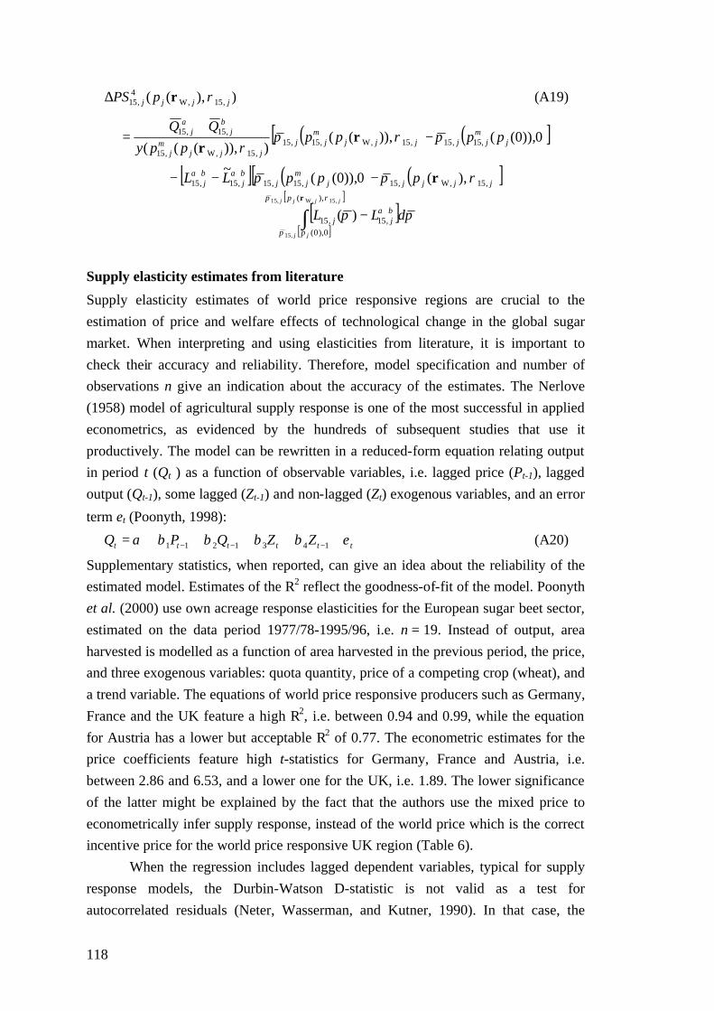
118

)),(( ,15,W4

,15 jjjj pPS ρρ∆ (A19)

( ) ( )[ ]0)),0(()),(())),((( ,15,15,15,W,15,15

,15,W,15

,15,15j

mjjjjj

mjj

jjjm

j

bj

aj pppp

ppyQQ

πρπρ

−+

= ρρ

[ ] ( ) ( )[ ]jjjjjm

jjbaj

baj pppLL ,15,W,15,15,15,15,15 ),(0)),0((

~ρππ ρ−−− ++

[ ][ ]

[ ]

∫ +−+jjjj

jj

p

p

bajj dLL

,15,W,15

,15

),(

0),0(,15,15 )(

ρπ

π

ππρ

Supply elasticity estimates from literature

Supply elasticity estimates of world price responsive regions are crucial to the estimation of price and welfare effects of technological change in the global sugar market. When interpreting and using elasticities from literature, it is important to check their accuracy and reliability. Therefore, model specification and number of observations n give an indication about the accuracy of the estimates. The Nerlove (1958) model of agricultural supply response is one of the most successful in applied econometrics, as evidenced by the hundreds of subsequent studies that use it productively. The model can be rewritten in a reduced-form equation relating output in period t (Qt ) as a function of observable variables, i.e. lagged price (Pt-1), lagged output (Qt-1), some lagged (Zt-1) and non-lagged (Zt) exogenous variables, and an error

term εt (Poonyth, 1998):

tttttt ZZQPQ εββββα +++++= −−− 1431211 (A20)

Supplementary statistics, when reported, can give an idea about the reliability of the estimated model. Estimates of the R2 reflect the goodness-of-fit of the model. Poonyth et al. (2000) use own acreage response elasticities for the European sugar beet sector, estimated on the data period 1977/78-1995/96, i.e. n = 19. Instead of output, area harvested is modelled as a function of area harvested in the previous period, the price, and three exogenous variables: quota quantity, price of a competing crop (wheat), and a trend variable. The equations of world price responsive producers such as Germany, France and the UK feature a high R2, i.e. between 0.94 and 0.99, while the equation for Austria has a lower but acceptable R2 of 0.77. The econometric estimates for the price coefficients feature high t-statistics for Germany, France and Austria, i.e. between 2.86 and 6.53, and a lower one for the UK, i.e. 1.89. The lower significance of the latter might be explained by the fact that the authors use the mixed price to econometrically infer supply response, instead of the world price which is the correct incentive price for the world price responsive UK region (Table 6).

When the regression includes lagged dependent variables, typical for supply response models, the Durbin-Watson D-statistic is not valid as a test for autocorrelated residuals (Neter, Wasserman, and Kutner, 1990). In that case, the

119

Durbin H-test can be considered as a valid alternative. For ‘large samples’ the test statistic has a standard normal distribution. Therefore, for a test of the null hypothesis of no autocorrelation against the two-sided alternative of autocorrelated errors, at a 5 % level, the decision rule is if -1.96 < H < +1.96 do not reject the null hypothesis. This condition is fulfilled for the relevant area elasticities since the equations of Germany, France, Austria and the UK feature H-statistics between 0.621 and 1.366 (Poonyth et al., 2000).

120

121

Appendix B: Structure of EUWABSIM

Software interaction

The latest version of the software package we developed to run our stochastic equilibrium displacement model is called EUWABSIM v12.0 (European Union Welfare effects of Agricultural Biotechnology Simulation Model). This package is a unique combination of three interlinked modules: a Microsoft Excel 2003 module, a Mathcad 2001i module, and an @Risk 4.5 module from Palisade Corporation (Figure 14). The originality and uniqueness of this combination lies in the interaction between the different modules. First, data on parameters coming from the literature, expert opinions and economic theory are stored in an Excel file, which is the base module of the package. Secondly, these data are sent to the Mathcad module. This mathematical module is installed as an add-in for Excel and enables presenting and calculating the mathematical model in a formal and transparent way, making it more convenient to modifications and error tracing instead of using Excel formulas embedded in individual cells. Thirdly, @Risk 4.5, also an add-in for Microsoft Excel, enables introducing prior distributions for parameters in the individual cells of an Excel sheet and hence consists of the uncertainty module of the model.

Triang(0, 0.29, 0.58)

0.0

0.5

1.0

1.5

2.0

2.5

3.0

3.5

-0.1

0.0

0.1

0.2

0.3

0.4

0.5

0.6

5.0% 90.0%0.0917 0.4883

Mathcad 2001i @Risk 4.5

parameters

define distributions

Iterations (10.000)

mathematical calculation of

simulation model

10.000 results

Exceldistribution

sensitivityscenarioanalyses

data from literature, experts, assumptions

Distribution for Total / AGGR/I27

Val

ues

in 1

0 ̂-9

Values in Billions

0123456789

0.9 0.9875 1.075 1.1625 1.250.9 0.9875 1.075 1.1625 1.25

5% 90% 5% 1.0039 1.1543

Figure 14: Schematic representation of the stochastic equilibrium displacement model EUWABSIM

122

For all parameters, @Risk randomly picks values from the defined prior distributions and sends them to the data cells in Excel. After each iteration generated by @Risk, the parameter values are changed in Excel, sent to and transformed by Mathcad and finally sent to Excel and @Risk again for analysis. The number of iterations can be chosen arbitrarily in @Risk. However, the more iterations, the more detailed are the estimates of the transformed prior distributions. @Risk collects the complete input-output table, which enables analysing the generated transformed prior distributions and conducting statistical, sensitivity and scenario analyses.

Solution for software interaction problem

There is one problem with the software interaction mentioned above. If one tries to link Mathcad output cells to other cells and link these cells to @Risk, the latter program does not wait for Mathcad to complete its calculation and collects the output of the previous iteration. This means that inputs i correspond with outputs i + 1. The resulting input-output table displays an incorrect correlation between inputs and outputs. Therefore, we contacted Palisade Corporation’s and Mathcad’s support team, subscribed to various discussion groups such as Mathcad-club, Mathcad Collaboratory, Mathcad discussion list and Contingency Analysis forum. We received a lot of feedback, although it did not yield a definitive solution. Finally, in late 2003 we discovered that the problem could be solved by avoiding linking any cells to Mathcad output cells. Therefore, we recommend the following procedure. Clear all Mathcad output cells before each simulation and add fresh @Risk output links to the cells. This will assure a correct interaction between Mathcad and @Risk. After each simulation, the output links have to be re-entered again, as they have been overwritten by Mathcad’s outputs. Although this interaction perfectly works, it is relatively slow. A single iteration takes 1.8 seconds to complete and if we conduct 10,000 iterations, a single simulation takes 5 hours of processor time with an Acer TravelMate 4100 with Intel® Pentium® M Processor at 1.3 ~ 1.6 GHz and 512 MB of RAM.

Mathematical module in EUWABSIM

The Mathcad module consists of a series of equations, linked to parameters collected in Excel which, on their turn, are linked to distributions defined in @Risk. Mathcad language is very convenient to work with as it uses standard algebraic notation. This makes modifications of EUWABSIM easy to implement, while structural model errors are quickly detected. The greatest advantage lies also in the possibility to specify multi-argument functions. As a result, one single transparent formula can handle a lot of calculations. In Figure 15 below we present the full Mathcad program language of EUWABSIM v12.0.

123

ρ j( ) if j 0 0,K

1 exp a b j⋅+( )+,

:=

testta p j,( ) τa0j 1 ξ0j+( )⋅QaEU QbEU+ Cj−

pi0 j, 1 ξ0j+( )⋅ QaEU QbEU+( )⋅p pw0j−( )⋅−:=

testtb p j,( ) τb0j 1 ξ0j+( )⋅QaEU QbEU+ Cj−

pi0 j, 1 ξ0j+( )⋅ QbEU⋅p pw0j−( )⋅−:=

test ξ p j,( ) ξ0j

QaEU QbEU+ Cj−

pi0 j, testta p j,( )⋅ QaEU QbEU+( )⋅ pi0 j, testtb p j,( )⋅ QbEU⋅+p pw0j−( )⋅−:=

τa p j,( ) if 0 testta p j,( )≤( ) 0.02< testta p j,( ), if 0 testtb p j,( )≤( ) 0.375< 0.02, 1 test ξ p j,( )+( ) 0.02⋅, , := τb p j,( ) if 0 testta p j,( )≤( ) 0.02< 0, if 0 testtb p j,( )≤( ) 0.375< testtb p j,( ), 1 test ξ p j,( )+( ) 0.375⋅, , := pa p i, j,( ) pii j, 1 τa p j,( )−( )⋅:=

pb p i, j,( ) pii j, 1 τa p j,( )− τb p j,( )−( )⋅:=

pm2 p i, j,( )Qai pa p i, j,( )⋅ Qbi pb p i, j,( )⋅+

Qai Qbi+:=

pm8 p i, j,( )Qai pa p i, j,( )⋅ Qbi pb p i, j,( )⋅+ qtot i j, Qai− Qbi−( ) p⋅+

qtot i j,:=

pm10 p i, j,( )Qai pa p i, j,( )⋅ Qbi pb p i, j,( )⋅+ 0.06 Qai Qbi+( )⋅ p⋅+

1.06 Qai Qbi+( )⋅:=

ip p i, j,( ) if φi j, 1≤ pa p i, j,( ), if φi j, 2 if i 8 pm8 p i, j,( ), if i 10 pm10 p i, j,( ), pb p i, j,( ),( ),( ), if,(,(:= if φi j, 3 if i 2 pm2 p i, j,( ), pb p i, j,( ),( ), p,( )))

Ai j, iπi

ip pw0j i, j,( ) yi j,⋅

1 η i+−:=

Gi j,

yi j,

ip pw0j i, j,( )ηi:=

κ j

Dj

ip pw0j 0, j,( )ε:=

θ i j,Ψ i iπi⋅

ip pw0j i, j,( ) yi j,⋅:=

λi j,

qtot i j,

iπi( )θi j,yi j,⋅

:=

R p r, i, j,( ) Ai j, r αi⋅+1 r βi⋅+( ) Gi j,⋅

1 η i+p

1 ηi+⋅+ r δwµi⋅−:=

L p r, i, j,( ) λi j, R p r, i, j,( )θi j,⋅:= Land v i, j,( ) λi j, v

θi j,⋅:=

Y p r, i, j,( ) 1 r βi⋅+( ) Gi j,⋅ pηi⋅:=

Q p r, i, j,( ) L p r, i, j,( ) Y p r, i, j,( )⋅:=

DROW p j,( ) κ j pε:=

QEU p r, j,( )

2

15

i

if φi j, 4 Q p r, i, j,( ), qtot i j,,( )∑=

:=

124

QROW p r, j,( ) if φ0 j, 6 Q p 0, 0, j,( ), qtot 0 j,,( ) if φ1 j, 5 Q p r, 1, j,( ), qtot 1 j,,( )+:=

pw j( ) pw0j 1 σ1 if j 1< 0,QEU pw0j ρ j( ), j,( ) qEUtot j−

qEUtot j,

⋅+

⋅:=

σ2 if j 2< 0,QEU pw0j 1− ρ j 1−( ), j 1−,( ) qEUtot j 1−−

qEUtot j 1−,

⋅+

DPSab i j,( )Qai

Y ip pw j( ) i, j,( ) ρ j( ), i, j,( ) R pa pw j( ) i, j,( ) ρ j( ), i, j,( ) R pa pw0j i, j,( ) 0, i, j,( )−( )⋅:=

DPSa i j,( ) if qtot i j, Qai<R pa pw0 j i, j,( ) 0, i, j,( )

R pa pw j( ) i, j,( ) ρ j( ), i, j,( )vLand v i, j,( )

⌠⌡

d, DPSab i j,( ),

:=

DPScd i j,( )Qai

Y ip pw0j i, j,( ) 0, i, j,( )Qai

Y ip pw j( ) i, j,( ) ρ j( ), i, j,( )−

R pa pw0j i, j,( ) 0, i, j,( ) R pb pw j( ) i, j,( ) ρ j( ), i, j,( )−( )⋅:=

DPSef i j,( )Qai Qbi+

Y ip pw j( ) i, j,( ) ρ j( ), i, j,( )Qai

Y ip pw0j i, j,( ) 0, i, j,( )−

R pb pw j( ) i, j,( ) ρ j( ), i, j,( ) R pb pw0j i, j,( ) 0, i, j,( )−( )⋅:=

DPSe i j,( ) if qtot i j, Qai Qbi+<

R pb pw0 j i, j,( ) 0, i, j,( )

R pb pw j( ) i, j,( ) ρ j( ), i, j,( )

vLand v i, j,( )Qai

Y ip pw0j i, j,( ) 0, i, j,( )−

⌠⌡

d, DPSef i j,( ),

:=

DPSgh i j,( )Qai Qbi+

Y ip pw0j i, j,( ) 0, i, j,( )Qai Qbi+

Y ip pw j( ) i, j,( ) ρ j( ), i, j,( )−

R pb pw0j i, j,( ) 0, i, j,( ) R pw j( ) ρ j( ), i, j,( )−( )⋅:=

DPSklm i j,( )

R pw0 j 0, i, j,( )

R pw j( ) ρ j( ), i, j,( )

vLand v i, j,( )Qai Qbi+

Y ip pw0j i, j,( ) 0, i, j,( )−

⌠⌡

d:=

DPS0 i j,( ) DPSa i j,( ):= DPS1 i j,( ) DPSab i j,( ):= DPS2 i j,( ) DPSab i j,( ) DPScd i j,( )− DPSe i j,( )+:= DPS3 i j,( ) DPSab i j,( ) DPScd i j,( )− DPSef i j,( )+:= DPS4 i j,( ) DPSab i j,( ) DPScd i j,( )− DPSef i j,( )+ DPSgh i j,( )− DPSklm i j,( )+:=

DPS5 i j,( )qtot i j,

Y pw j( ) ρ j( ), i, j,( ) R pw j( ) ρ j( ), i, j,( ) R pw0j 0, i, j,( )−( )⋅:=

DPS6 i j,( )R pw0 j 0, i, j,( )

R pw j( ) ρ j( ), i, j,( )vLand v i, j,( )

⌠⌡

d:=

DPS28 i j,( )qtot i j,

Y ip pw j( ) i, j,( ) ρ j( ), i, j,( ) R pm8 pw j( ) i, j,( ) ρ j( ), i, j,( ) R pm8 pw0j i, j,( ) 0, i, j,( )−( )⋅:=

DPS210 i j,( )1.06 Qai Qbi+( )⋅


DPS32 i j,( )Qai Qbi+


125

DPS415 i j,( ) DPS32 i j,( ) DPSklm i j,( )+:=

Qai Qbi+

Y ip pw0j i, j,( ) 0, i, j,( )Qai Qbi+

Y ip pw j( ) i, j,( ) ρ j( ), i, j,( )−

R pm2 pw0j i, j,( ) 0, i, j,( ) R pw j( ) ρ j( ), i, j,( )−( )⋅−

DPS2all i j,( ) if i 8 DPS28 i j,( ), if i 10 DPS210i j,( ), DPS2 i j,( ),( ),( ):= DPS3all i j,( ) if i 2 DPS32 i j,( ), DPS3 i j,( ),( ):= DPS4all i j,( ) if i 15 DPS415 i j,( ), DPS4 i j,( ),( ):= DPS s i, j,( ) if s 0 DPS0 i j,( ), 0,( ) if s 1 DPS1 i j,( ), 0,( )+ if s 2 DPS2all i j,( ), 0,( )+:=

if s 3 DPS3all i j,( ), 0,( )+ if s 4 DPS4all i j,( ), 0,( )+ if s 5 DPS5 i j,( ), 0,( )+ if s 6 DPS6 i j,( ), 0,( )+ ∆PS i j,( ) DPS φi j, i, j,( ):=

∆PSEU j( )

2

15

i

∆PS i j,( )∑=

:=

∆PSROW j( )

0

1

i

∆PS i j,( )∑=

:=

∆CSEU j( ) 0:=

∆CSROW j( )pw j( )

pw0 j

pDROW p j,( )⌠⌡

d:=

Π j( )

0

15

i

ρ j( ) if φi j, 4 φi j, 6∨ L pw j( ) ρ j( ), i, j,( ),qtot i j,

Y ip pw j( ) i, j,( ) ρ j( ), i, j,( ),

⋅ δwµi⋅∑=

:=

TOT j( ) ∆PSEU j( ) ∆CSEU j( )+ ∆PSROW j( )+ ∆CSROW j( )+ Π j( )+:=

LS0 i( )

1

5

j

qtot i j,

yi j,∑=

:=

LS1 i( )

1

5

j

if φi j, 4 φi j, 6∨ L pw j( ) ρ j( ), i, j,( ),qtot i j,

Y ip pw j( ) i, j,( ) ρ j( ), i, j,( ),

∑

=

:=

LSR i( )LS1 i( ) LS0 i( )−

LS0 i( ):=

LS0EU

2

15

i

LS0 i( )∑=

:=

LS0ROW

0

1

i

LS0 i( )∑=

:=

LS0W

0

15

i

LS0 i( )∑=

:=

LS1EU

2

15

i

LS1 i( )∑=

:=

LS1ROW

0

1

i

LS1 i( )∑=

:=

LS1W

0

15

i

LS1 i( )∑=

:=

LSREULS1EU LS0EU−

LS0EU:=

LSRROW

LS1ROW LS0ROW−LS0ROW

:=

LSRWLS1W LS0W−

LS0W:=

Figure 15: Program language of the Mathcad module in EUWABSIM v12.0

126

127

References Abel, A.B., and J.C. Eberley. “An exact solution for the investment and value of a firm facing

uncertainty, adjustment costs, and irreversibility.” Journal of Economic Dynamics and Control 21(1997):831-52.

Acquaye, A.K.A., and G. Traxler. “Monopoly power, price discrimination, and access to biotechnology innovations.” AgBioForum 8(2005).

Agra Europe “EU food agency must be more transparent over GMOs.” Agra Europe 2203(April 2006a):EP/1-EP/2.

--- “Science beaten by emotion in GMO co-existence debate.” Agra Europe 2202(April 2006b):A/1-A/2.

Alcalde, E. “Compa CB: Resultados de los agricultores con el primer maíz resistente al taladro.” Actas del 6.° Symposium Nacional de Sanidad Vegetal. pp. 469-477. Sevilla: Consejería de Agricultura y Pesca, Junta de Andalucía, 1999.

---, “Co-existence of GM maize in Spain.” Paper presented at EU’s Round Table on Co-existence of GM and non-GM agriculture: A missed opportunity, Brussels, 24 April 2003.

Allen, D.W., and D. Lueck. “The nature of the farm.” Journal of Law and Economics 41(October 1998):343-86.

Alston, J.M., C. Chan-Kang, M.C. Marra, P.G. Pardey, and T. Wyatt. “A meta-analysis of rates of return to agricultural R&D: Ex pede herculem?” Research Report, International Food Policy Research Institute, Washington, DC, 2000.

Alston, J.M., G.W. Edwards, and J.W. Freebairn. “Market distortions and benefits from research.” American Journal of Agricultural Economics 70(1988):281-88.

Alston, J.M., J. Hyde, M.C. Marra, and P.D. Mitchell. “An ex ante analysis of the benefits from the adoption of corn rootworm resistant transgenic corn technology.” AgBioForum 5(2002):71-84.

Alston, J.M., and D.M. Larson. “Hicksian vs Marshallian welfare measures: Why do we do what we do?” American Journal of Agricultural Economics 75(August 1993):764-69.

Alston, J.M., G.W. Norton, and P.G. Pardey. Science under scarcity: principles and practice of agricultural research evaluation and priority setting. Ithaca, NY: Cornell University Press, 1995.

Antle, J.M., and P. Pingali. “Pesticides, productivity and farmers health: A Philippine case study.” American Journal of Agricultural Economics 76(1994):418-30.

Arrow, K., and A.C. Fisher. “Environmental preservation, uncertainty, and irreversibility.” Quarterly Journal of Economics 88(1974):312-19.

Arrow, K.J. “Economic welfare and the allocation of resources for invention.” The rate and direction of inventive activity: economic and social factors. Nelson, R.R., ed., Princeton, NJ: Princeton University Press, 1962.

Bartsch, D., M. Lehnen, J. Clegg, M. Pohl-Orf, I. Shuphan, and N.C. Ellstrand. “Impact of gene flow from cultivated beet on genetic diversity of wild sea beet populations.” Molecular Ecology 8(1999):1733-41.

Bartsch, D., and I. Schuphan. “Lessons we can learn from ecological biosafety research.” Journal of Biotechnology 98(September 2002):71-77.

Beattie, B.R. “Science under scarcity (Review).” American Journal of Agricultural Economics 77(November 1995):1064-81.

Beghin, J.C., B. El Osta, J.R. Cherlow, and S. Mohanty. “The cost of the U.S. sugar program revisited.” Contemporary Economic Policy 21(January 2003):106-16.

Benbrook, C.M. “The farm-level economic impacts of Bt corn from 1996 through 2001: An independent national assessment.” Ag BioTech InfoNet Technical Paper, Benbrook Consulting Services, Sandpoint, Idaho, 2001.

Bhagwati, J.N. “Immiserizing growth: A geometrical note.” Review of Economic Studies 25(1958):201-5.

Bijman, J. “Advanta: worldwide challenges.” AgBioForum 4(2001a):34-39. --- “KWS: going beyond sugar beet.” AgBioForum 4(2001b):46-51. Bijman, J., and J. Tait. “Public policies influencing innovation in the agrochemical, biotechnology

and seed industries.” Science and Public Policy 29(August 2000):245-51. Bock, A.-K., K. Lheureux, M. Libeau-Dulos, H. Nilsagård, and E. Rodriguez-Cerezo. “Scenarios

for co-existence of genetically modified, conventional and organic crops in European agriculture.” Technical Report, n° EUR 20394EN, European Communities, Brussels, 2002.

Bohn, M., R.C. Kreps, D. Klein, and A.E. Melchinger. “Damage and grain yield losses caused by European corn borer (Lepidoptera: Pyralidae) in early maturing European maize hybrids.” Journal of Economic Entomology 92(June 1999):723-31.

128

Bromley, D.W., “The emergence and evolution of natural resource economics: 1950-2000.” Paper presented at Frontiers in Resource and Rural Economics: Rural-Urban Interplay and Nature-Human Interactions,” in honor of Emery N. Castle, Oregon State University, Corvallis, Oregon, October 5-7 2005.

Brookes, G. “The farm level impact of using Bt maize in Spain.”, Brookes West, Kent, UK, 2002. --- “The farm-level impact of herbicide-tolerant soybeans in Romania.” AgBioForum 8(2005):235-41. Brown, M.B., and A.B. Forsythe. “Robust tests for the equality of variances.” Journal of the

American Statistical Association 69(1974):364-67. Bückmann, H., J. Petersen, G. Schlinker, and B. Märländer. “Weed control in genetically modified

sugar beet - Two years experiences of a field trial series in Germany.” Zeitschrift für PflanzenKrankheit und PflanzenSchutzung 17(2000):353-62.

Bureau, J.-C., H. Guyomard, L. Morin, and V. Réquillart. “Quota mobility in the European sugar regime.” European Review of Agricultural Economics 24(1997):1-30.

Burgener, P.A., D. M. Feuz, and R. G. Wilson., “The economics of transgenic sugarbeet production.” Paper presented at Western Agricultural Economics Association Annual Meetings, Vancouver, Canada 2000.

Burton, M., D. Rigby, T. Young, and S. James. “Consumers attitudes to genetically modified organisms in food in the UK.” European Review of Agricultural Economics 28(2001):479-98.

Campbell, J.Y., A.W. Lo, and A.C. MacKinlay. The econometrics of financial markets. Princeton, USA: Princeton University Press, 1997.

Chipman, J.S., and J.C. Moore. “The new welfare economics, 1939-1974.” International Economic Review 19(October 1978):581-84.

Coghlan, A. “GM sugar beet ‘far more environmentally friendly’.” New Scientist(December 2003). Combette, P., E. Giraud-Heraud, and V. Réquillart. “La politique sucrière européenne après les

accords du GATT: Une analyse de quelques scénarios d’évolution.” Economie et Prévision 127(1997):1-13.

Confédération des Betteraviers Belges, Personal communication, 18-6-2002. Cordero, A., R.A. Malvar, A. Butrón, P. Revilla, P. Velasco, and A. Ordás. “Population dynamics

and life-cycle of corn borers in South Atlantic European coast.” Maydica 43(1998):5-12. Coyette, B., F. Tencalla, I. Brants, and Y. Fichet. “Effect of introducing glyphosate-tolerant sugar

beet on pesticide usage in Europe.” Pesticide Outlook 13(October 2002):219-23. Crawley, M.J., S.L. Brown, R.S. Hails, D.D. Kohn, and M. Rees. “Biotechnology: Transgenic crops

in natural habitats.” Nature 409(2001):682-83. Davis, G.C., and M.C. Espinoza. “A unified approach to sensitivity analysis in equilibrium

displacement models.” American Journal of Agricultural Economics 80(1998):868-79. Davis, G.C., and M.C. Espinoza. “A unified approach to sensitivity analysis in equilibrium

displacement models: Reply.” American Journal of Agricultural Economics 82(2000):241-43. de Borchgrave, R., Personal communication, 10-4-2006. de Borchgrave, R., N.G. Kalaitzandonakes, A. Galvao Gomes, and B.H. de Frahan. Economics of

non-GM food/feed supply chains in Europe. London, UK: AgraEurope, 2003. Demont, M., E. Mathijs, and E. Tollens. “Impact of new technologies on agricultural production

systems: The cases of agricultural biotechnology and automatic milking.” New technologies and sustainability. Bouquiaux, J.-M., L. Lauwers, and J. Viaene, ed., pp. 11-38. Brussels: CLE-CEA, 2001.

Demont, M., and E. Tollens. “Ex ante welfare effects of agricultural biotechnology in the European Union: The case of transgenic herbicide tolerant sugarbeet.” The regulation of agricultural biotechnology. Evenson, R.E., and V. Santaniello, ed., pp. 239-255. Wallingford, UK: CAB International, 2004.

--- “First impact of biotechnology in the EU: Bt maize adoption in Spain.” Annals of Applied Biology 145(2004):197-207.

Demont, M., J. Wesseler, and E. Tollens. “Biodiversity versus transgenic sugar beet: The one Euro question.” European Review of Agricultural Economics 31(2004):1-18.

--- “Irreversible costs and benefits of transgenic crops: What are they?” Environmental costs and benefits of transgenic crops. Wesseler, J., ed., pp. 113-122. Dordrecht, NL: Springer, 2005.

Desplanque, B., N. Hautekeete, and H. Van Dijk. “Transgenic weed beets: Possible, probable, avoidable?” Journal of Applied Ecology 39(August 2002):561-71.

Devadoss, S., and J. Kropf. “Impacts of trade liberalizations under the Uruguay Round on the world sugar market.” Agricultural Economics 15(November 1996):83-96.

129

Devos, Y., D. Reheul, and A. De Schrijver. “The co-existence between transgenic and non-transgenic maize in the European Union: a focus on pollen flow and cross-fertilization.” Environmental Biosafety Research 4(2005):71-87.

DeVuyst, C.S., and C.J. Wachenheim. “American Crystal Sugar: Genetically enhanced sugarbeets?” Review of Agricultural Economics 27(2005):105-16.

Dewar, A.M. “Control of pests by manipulation of weeds in GM herbicide-tolerant sugar beet.” IIRB 63rd Congress Proceedings. pp. 187-198. Brussels: IIRB, 2000.

Dixit, A., and R.S. Pindyck. Investment under uncertainty. Princeton: Princeton University Press, 1994.

Duff, A., “Economic aspects of GM beet and cane.” Paper presented at Agricultural Outlook Forum 1999, Arlington VA, 22-23 February 1999.

EEA “Household number and size.” Indicator Fact Sheet Signals 2001, n° YIR01HH03, European Environment Agency, Copenhagen, 2001.

European Commission “Sugar.” CAP Working Notes 1996/97, Office for Official Publications of the European Communities Luxembourg, 1996.

--- The agricultural situation in the European Union: 1998 report. Luxembourg: Office for Official Publications of the European Communities, 1999.

--- “Commission Recommendation of 23 July 2003 on guidelines for the development of national strategies and best practices to ensure the coexistence of genetically modified crops with conventional and organic farming.” Official Journal of the European Communities L189(July 2003a):0036-47.

--- “Sugar: International analysis, production structures within the EU.”, n° 04/177, Commission of the European Communities, Brussels, 2003b.

--- “Proposal for a Council Regulation on the common organisation of the markets in the sugar sector.”, n° COM(2005) 263 final, Commission of the European Communities, Brussels, 2005.

--- Deliberate releases and placing on the EU market of genetically modified organisms (GMOs). Brussels: Commission of the European Communities, 2006a.

--- Farm accountancy data network. Brussels: FADN EC-DG Agri/G3, 2006b. Eurostat SPEL/EU data for agriculture on CD-ROM: 1973-1998 data. Luxembourg: Office for

Official Publications of the European Communities, 1999. --- Plant protection in the EU - Consumption of plant protection products in the European Union.

Luxembourg: Office of Official Publications of the European Communities, 2000. --- AGRIS application and data for agriculture: Data 1973-2003. Luxembourg: Office for Official

Publications of the European Communities, 2003. F.O.Licht World sugar statistics 2002. Kent: F.O.Licht, 2001. Falck-Zepeda, J.B., G. Traxler, and R.G. Nelson. “Rent creation and distribution from the first three

years of planting Bt cotton.” ISAAA Briefs, n° 14, ISAAA, Ithaca, NY, 1999. --- “Rent creation and distribution from biotechnology innovations: The case of Bt cotton and

herbicide-tolerant soybeans in 1997.” Agribusiness 16(2000a):21-32. --- “Surplus distribution from the introduction of a biotechnology innovation.” American Journal of

Agricultural Economics 82(May 2000b):360-369. FAO FAOSTAT agriculture data. Rome: FAO, 2006. Feder, G., R.E. Just, and D. Zilberman. “Adoption of agricultural innovations in developing

countries: A survey.” Economic Development and Cultural Change 33(1985):255-98. Fernández-Anero, J., C. Novillo, and J. Costa. “MaisGard protección contra taladros en toda la

planta, durante toda la campaña. Resultados en España 1997-1998.” Actas del 6.° Symposium Nacional de Sanidad Vegetal. pp. 447-455. Sevilla: Consejería de Agricultura y Pesca, Junta de Andalucía, 1999.

Fernandez-Cornejo, J., C. Hendricks, and A. Mishra. “Technology adoption and off-farm household income: The case of herbicide-tolerant soybeans.” Journal of Agricultural and Applied Economics 37(December 2005):549-63.

Fernandez-Cornejo, J., and W.D. McBride. “Adoption of bioengineered crops.” Agricultural Economic Report, n° AER810, Economic Research Service, USDA, Washington, 2002.

Fisher, A.C. “Investment under uncertainty and option value in environmental economics.” Resource and Energy Economics 22(2000):197-204.

Flannery, M.-L., F.S. Thorne, P.W. Kelly, and E. Mullins. “An economic cost-benefit analysis of GM crop cultivation: An Irish case study.” AgBioForum 7(2004):149-57.

Frandsen, S.E., H.G. Jensen, W. Yu, and A. Walter-Jørgensen. “Reform of EU sugar policy: Price cuts versus quota reductions.” European Review of Agricultural Economics 30(2003):1-26.

130

Frisvold, G.B., J. Sullivan, and A. Raneses. “Genetic improvements in major US crops: The size and distribution of benefits.” Agricultural Economics 28(2003):109-19.

Frisvold, G.B., and R. Tronstad. “Economic effects of Bt cotton adoption and the impact of government programs.” The economic and environmental impacts of agbiotech: A global perspective. Kalaitzandonakes, N.G., ed., pp. 261-286. New York: Kluwer Academic/Plenum Publishers, 2003.

Gaillard, S. “L’industrialisation de la culture du maïs-grain en France 1945-1985: un itinéraire particulier.” Economie Rurale 187(October 1988):25-32.

Gebhard, F., and K. Smalla. “Monitoring field releases of genetically modified sugar beets for persistence of transgenic plant DNA and horizontal gene transfer.” FEMS Microbiology Ecology 28(1999):261-72.

Gianessi, L.P., and J.E. Carpenter. “Agricultural biotechnology: Insect control benefits.”, National Center for Food and Agricultural Policy (NCFAP), Washington, 1999.

--- “Agricultural Biotechnology: Benefits of Transgenic Soybeans.”, National Center for Food and Agricultural Policy (NCFAP), Washington, 2000.

Gianessi, L.P., S. Sankula, and N. Reigner. “Plant biotechnology: Potential impact for improving pest management in European agriculture, maize case study.”, National Center for Food and Agricultural Policy, Washington, DC, 2003a.

--- “Plant biotechnology: Potential impact for improving pest management in European agriculture, sugarbeet case study.”, National Center for Food and Agricultural Policy, Washington, DC, 2003b.

Gianessi, L.P., C.S. Silvers, S. Sankula, and J.E. Carpenter. “Plant biotechnology current and potential impact for improving pest management in U.S. agriculture: An analysis of 40 case studies.”, National Center for Food and Agricultural Policy (NCFAP), Washington, 2002.

Gohin, A., and J.-C. Bureau. “Modelling the EU sugar supply to assess sectoral policy reforms.” European Review of Agricultural Economics 33(2006):223-47.

Gouse, M., C.E. Pray, and D.E. Schimmelpfennig. “The distribution of benefits from Bt cotton adoption in South Africa.” AgBioForum 7(2004):187-94.

Greenpeace “EU suppresses study showing genetically engineered crops add high costs for all farmers and threaten organic.” Greenpeace Press Release(May 2002).

Griffiths, W., and X.Y. Zhao. “A unified approach to sensitivity analysis in equilibrium displacement models: Comment.” American Journal of Agricultural Economics 82(2000):236-40.

Griliches, Z. “Hybrid corn: An exploration in the economics of technological change.” Econometrica 25(October 1957):501-22.

--- “Research costs and social returns: Hybrid corn and related innovations.” Journal of Political Economics 66(October 1958):419-31.

Gura, T. “The battlefields of Britain.” Nature 412(August 2001):760-763. Henry, C. “Investment decision under uncertainty: The irreversibility effect.” American Economic

Review 64(1974):1006-12. Hermann, O. “Enquête sur les parasites et sur le coût des traitements phytosanitaires dans la culture de

la betterave sucrière en Europe.” C.I.B.E. XXXVIth Congress Proceedings. pp. 1-8. Paris: C.I.B.E., 1996.

--- “Enquête sur le coût de la lutte phytosanitaire dans la culture de la betterave sucrière en Europe.” IIRB 60th Congress Proceedings. pp. 469-475. Brussels: IIRB, 1997.

Horowitz, J.K., and E. Lichtenberg. “Risk-reducing and risk-increasing effects of pesticides.” Journal of Agricultural Economics 45(1994):82-89.

Hurley, T.M., P.D. Mitchell, and M.E. Rice. “Risk and the value of Bt corn.” American Journal of Agricultural Economics 86(2004):345-58.

Hyde, J., M.A. Martin, P.V. Preckel, and C.R. Edwards. “The economics of Bt corn: Valuing protection from the European corn borer.” Review of Agricultural Economics 21(1999):442-54.

IMF “World economic outlook: Recessions and recoveries.” World Economic and Financial Surveys, International Monetary Fund, Washington, 2002.

James, C. “Global status of transgenic crops in 1997.” ISAAA Briefs, n° 5, ISAAA, Ithaca, NY, 1997. --- “Global review of commercialised transgenic crops: 1998.” ISAAA Briefs, n° 8, ISAAA, Ithaca,

NY, 1998. --- “Global status of commercialized transgenic crops: 1999.” ISAAA Briefs, n° 17, ISAAA, Ithaca,

NY, 2000. --- “Global review of commercialized transgenic crops: 2000.” ISAAA Briefs, n° 23, ISAAA, Ithaca,

NY, 2001. --- “Global review of commercialized transgenic crops: 2001 - Feature: Bt cotton.” ISAAA Briefs, n°

26, ISAAA, NY, 2002.

131

--- “Global review of commercialized transgenic crops: 2002 - Feature: Bt maize.” ISAAA Briefs, n° 29, ISAAA, Ithaca, NY, 2003a.

--- “Global status of commercialized transgenic crops: 2003 - Preview.” ISAAA Briefs, n° 30, ISAAA, Ithaca, NY, 2003b.

--- “Global status of commercialized biotech/GM crops: 2005 - Preview.” ISAAA Briefs, n° 34, ISAAA, Ithaca, NY, 2006.

Jansens, S., A. Van Vliet, C. Dickburt, L. Buysse, C. Piens, B. Saey, A. De Wulf, V. Gosselé, A. Paez, E. Göbel, and M. Peferoen. “Transgenic corn expressing a Cry9C insecticidal protein from Bacillus thuringiensis protected from European corn borer damage.” Crop Science 37(1997):1616-24.

Just, R.E., D.L. Hueth, and A. Schmitz. Applied welfare economics and public policy. Englewood Cliffs NJ: Prentice-Hall Inc., 1982.

Kergoat, P.-Y. “Bénéfices agronomiques et environnementaux du maïs transgénique MON810 qui est efficace contre la pyrale et la sésamie.” Annales ANPP, Cinquième Conférence Internationale sur les Ravageurs en Agriculture, Montpellier, December 7-9. pp. 37-44. Paris: Association Nationale de Protection des Plantes, 1999.

Kilman, S. “Food industry shuns bioengineered sugar.” Wall Street Journal(April 2001). Kim, K., and J.-P. Chavas. “Technological change and risk management: An application to the

economics of corn production.” Agricultural Economics 29(2003):125-238. Kniss, A.R., R.G. Wilson, A.R. Martin, P.A. Burgener, and D.M. Feuz. “Economic evaluation of

glyphosate-resistant and conventional sugar beet.” Weed Technology 18(2004):388-96. Labatte, J.-M., S. Meusnier, A. Migeon, J. Chaufaux, Y. Couteaudier, G. Riba, and B. Got. “Field

evaluation of and modeling the impact of three control methods on the larval dynamics of Ostrinia nubilalis (Lepidoptera: Pyralidae).” Journal of Economic Entomology 89(August 1996):852-62.

Lapan, H.E., and G. Moschini. “Incomplete adoption of a superior innovation.” Economica 67(2000):525-42.

Le Stum, H., and D. Camaret. “Coûts de production du blé tendre et du maïs en France.” Perspectives Agricoles 138(July 1989):19-30.

Lekakis, J.N., and C. Pantzios. “Agricultural liberalization and the environment in Southern Europe: The role of the supply side.” Applied Economics Letters 6(1999):453-58.

Lemarié, S., M. Desquilbet, A. Diemer, S. Marette, F. Levert, M. Carrère, and D.S. Bullock. “Les répartitions possibles entre les acteurs de la filière agro-alimentaire des gains éventuels tirés des plantes transgéniques en France.” Rapport au commissariat Général du Plan, INRA, Rennes, 2001.

Lemarié, S., and S. Marette. “Substitution and complementarities in the Biotechnology and pesticide markets: A theoretical framework.” The economic and environmental impacts of agbiotech: A global perspective. Kalaitzandonakes, N.G., ed., pp. 287-305. New York: Kluwer Academic/Plenum Publishers, 2003.

Levene, H. “Robust tests for equality of variance.” Contributions to Probability and Statistics: Essays in Honor of Harold Hotelling. Olkin, I., S.G. Ghurye, W. Hoeffding, W.G. Madow, and H.B. Mann, ed., pp. 278-292. Stanford, CA: Stanford University Press, 1960.

MAPA Encuesta sobre Superficies y Rendimientos de Cultivos, resultados de la encuesta de superficies 2002. Madrid: Ministerio de Agricultura, Pesca y Alimentación, 2003.

--- Encuesta sobre Superficies y Rendimientos de Cultivos, resultados de la encuesta de superficies 2003. Madrid: Ministerio de Agricultura, Pesca y Alimentación, 2004.

Märländer, B. “Weed control in sugar beet using genetically modified herbicide-tolerant varieties - A review of the economics for cultivation in Europe.” Journal of Agronomy & Crop Science 191(2005):64-74.

Märländer, B., and H. Bückmann. “Genetically modified varieties in Germany - Status and prospects with special respect of a sustainable sugar beet cultivation.” Zuckerindustrie 124(1999):943-46.

Marra, M.C., P.G. Pardey, and J.M. Alston. “The payoffs to agricultural biotechnology: An assessment of the evidence.” EPTD Discussion Paper, n° 87, IFPRI, Washington, 2002.

Marra, M.C., N.E. Piggott, and G.A. Carlson. “The net benefits, including convenience, of Roundup Ready® soybeans: Results from a national survey.” Technical Bulletin, n° 2004-3, NSF Center for Integrated Pest Management, Raleigh, NC, 2004.

Marra, M.C., N.E. Piggott, and O. Sydorovych. “The impact of herbicide tolerant crops on North Carolina farmers.” NC State Economist March/April(2005):1-4.

Mason, C.E., M.E. Rice, D.D. Calvin, J.W. Van Duyn, W.B. Showers, W.D. Hutchison, J.F. Witkowski, R.A. Higgins, D.W. Onstad, and G.P. Dively. “European corn borer: Ecology and management.” North Central Regional Extension Publication, n° 327, Iowa State University, Ames, IA, 1996.

132

May, M.J. “Efficiency and selectivity of RR and LL weed control techniques compared to classical weed control systems.” IIRB 63rd Congress Proceedings. pp. 163-170. Brussels: IIRB, 2000.

--- “Economic consequences for UK farmers of growing GM herbicide tolerant sugar beet.” Annals of Applied Biology 142(2003):41-48.

McDonald, R., and D. Siegel. “The value of waiting to invest.” Quarterly Journal of Economics 101(1986):707-28.

McDougall, J., and M. Phillips. “The impact of agricultural biotechnology on the conventional agrochemical market.” The economic and environmental impacts of agbiotech: A global perspective. Kalaitzandonakes, N.G., ed., pp. 19-41. New York: Kluwer Academic/Plenum Publishers, 2003.

Messéan, A., F. Angevin, M. Gómez-Barbero, K. Menrad, and E. Rodríguez-Cerezo. “New case studies on the coexistence of GM and non-GM crops in European agriculture.” Technical Report, n° EUR 22102 EN, European Communities, 2006.

Mitchell, P. D. and Hurley, T. M., Personal communication, 6-8-2001. Monsanto, Personal communication, 19-6-2002. Moravskoslezské cukrovary, Personal communication, 13-4-2006. Morel, B., S. Farrow, F. Wu, and E. Casman. “Pesticide resistance, the precautionary principle, and

the regulation of Bt corn: real option and rational option approaches to decision-making.” Battling Resistance to Antibiotics. An Economic Approach. Laxminarayan, R., ed., pp. 184-213. Washington, DC: Resources for the Future, 2003.

Moschini, G., H. Bulut, and L. Cembalo. “On the segregation of genetically modified, conventional, and organic products in European agriculture: a multi-market equilibrium analysis.” Journal of Agricultural Economics 56(2005):347-72.

Moschini, G., and H.E. Lapan. “Intellectual property rights and the welfare effects of agricultural R&D.” American Journal of Agricultural Economics 79(1997):1229-42.

Moschini, G., H.E. Lapan, and A. Sobolevsky. “Roundup Ready soybeans and welfare effects in the soybean complex.” Agribusiness 16(2000):33-55.

Nerlove, M.L. “Distributed lags and estimation of long-run supply and demand elasticities: Theoretical considerations.” Journal of Farm Economics 40(May 1958):301-11.

Neter, J., W. Wasserman, and M.H. Kutner. Applied linear statistical models: Regression, analysis of variance, and experimental designs., 3 ed. Illinois, Massachusetts and Australia: IRWIN, 1990.

Nielsen, C.P., and K. Anderson. “Global market effects of alternative European responses to genetically modified organisms.” Weltwertschaftliches Archiv 137(2001):320-346.

Noussair, C., S. Robin, and B. Ruffieux. “Do consumers really refuse to buy genetically modified food?” The Economic Journal 114(January 2004):102-20.

O’Shea, L., and A. Ulph. “Providing the correct incentives for genetic modification.” The Economics of Managing Biotechnologies. Swanson, T., ed., pp. 129-143. London: Kluwer Academic Publishers, 2002.

OECD, “Assessing agricultural biotechnology in emerging economies.” Paper presented at OECD Global Forum on the Knowledge Economy: Modern Agricultural Biotechnology in Non-Member Countries, Paris, 18-19 November 2003a.

--- “Developments in Spain.” OECD Economic Outlook, n° 74, OECD, Paris, 2003b. Oehmke, J.F., and E.W. Crawford. “The sensitivity of returns to research calculations to supply

elasticity.” American Journal of Agricultural Economics 84(May 2002):366-69. Oehmke, J.F., and C.A. Wolf. “Why is Monsanto leaving money on the table? Monopoly pricing and

technology valuation distributions with heterogeneous adopters.” Journal of Agricultural and Applied Economics 36(2004):705-18.

Ostlie, K.R., W.D. Hutchison, and R.L. Hellmich. “Bt corn and European corn borer.” North Central Regional Extension Publication, n° NCR 602, University of Minnesota, 1997.

Palisade Corporation Guide to using @RISK risk analysis and simulation add-In for Microsoft® Excel version 4.5. Newfield, NY: Palisade Corporation, 2002.

Pannell, D.J. “Pests and pesticides, risk and risk aversion.” Agricultural Economics 5(1991):361-83. Pemsl, D., H. Waibel, and A.P. Gutierrez. “Why do some Bt-cotton farmers in China continue to use

high levels of pesticides?” International Journal of Agricultural Sustainability 3(2005):44-56. PG Economics Ltd. “Consultancy support for the analysis of the impact of GM crops on UK farm

profitability.”, Strategy Unit, London, 2003. Phillips, P.W.B. “The economic impact of herbicide tolerant canola in Canada.” The economic and

environmental impacts of agbiotech: A global perspective. Kalaitzandonakes, N.G., ed., pp. 119-139. New York: Kluwer Academic/Plenum Publishers, 2003.

133

Phipps, R.H., and J.R. Park. “Environmental benefits of genetically modified crops: Global and European perspectives on their ability to reduce pesticide use.” Journal of Animal and Feed Sciences 11(2002):1-18.

Pimentel, D., H. Acquay, M. Biltonen, P. Rice, M. Silva, J. Nelson, V. Lipner, S. Giordano, A. Horowitz, and M. D’Amore. “Environmental and economic costs of pesticide use.” BioScience 42(November 1992):750-759.

Pindyck, R.S. “Irreversibilities and the timing of environmental policy.” Resource and Energy Economics 22(2000):233-59.

Pingali, P.L. 1999/2000 World maize facts and trends. Meeting world maize needs: Technological opportunities and priorities for the public sector. Mexico, D.F.: CIMMYT, 2001.

Pohl-Orf, M., U. Brand, S. Driessen, P.R. Hesse, M. Lehnen, C. Morak, T. Muecher, C. Saeglitz, C. von Soosten, and D. Bartsch. “Overwintering of genetically modified sugar beet, Beta vulgaris L. subsp. vulgaris, as a source for dispersal of transgenic pollen.” Euphytica 108(1999):181-86.

Poonyth, D. “A structural econometric model of European Union sugar industry and the potential implications of the GATT WTO.” Ph.D. Dissertation, Faculty of the Graduate School, University of Missouri-Columbia, 1998.

Poonyth, D., P. Westhoff, A. Womack, and G. Adams. “Impacts of WTO restrictions on subsidized EU sugar exports.” Agricultural Economics 22(April 2000):233-45.

Pray, C.E., D. Ma, J. Huang, and F. Qiao. “Impact of Bt cotton in China.” World Development 29(2001):813-25.

Pretty, J.N., C. Brett, D. Gee, R.E. Hine, C.F. Mason, J.I.L. Morison, H. Raven, M.D. Rayment, and G. van der Bijl. “An assessment of the total external costs of UK agriculture.” Agricultural Systems 65(2000):113-36.

Pretty, J., C. Brett, D. Gee, R. Hine, C. Mason, J. Morison, M. Rayment, G. van der Vijl, and T. Dobbs. “Policy challenges and priorities for internalizing the externalities of modern agriculture.” Journal of Environmental Planning and Management 44(2001):263-83.

Price, G.K., W. Lin, J.B. Falck-Zepeda, and J. Fernandez-Cornejo. “Size and distribution of market benefits from adopting biotech crops.” Technical Bulletin, n° 1906, Economic Research Service, USDA, Washington, 2003.

Qaim, M. “Potential benefits of agricultural biotechnology: An example from the Mexican potato sector.” Review of Agricultural Economics 21(1999):390-408.

--- “Bt cotton in India: Field trial results and economic projections.” World Development 31(2003):2115-27.

--- “Agricultural biotechnology adoption in developing countries.” American Journal of Agricultural Economics 87(2005):1317-24.

Qaim, M., and A. de Janvry. “Genetically modified crops, corporate pricing strategies, and farmers’ adoption: The case of Bt cotton in Argentina.” American Journal of Agricultural Economics 85(November 2003):814-28.

Qaim, M., and G. Traxler. “Roundup Ready soybeans in Argentina: farm level, environmental, and welfare effects.” Agricultural Economics 32(2005):73-86.

Rasmusson, A. “Vad finns i betodlarens ryggsack? [What is in the beet-growers rucksack?].” Betodlaren 4(1998):21-23.

Rice, C.A., A. Mesbah, and S.D. Miller. “Economic evaluation of weed management systems in sugarbeets.” Proceedings of the American Society of Sugar Beet Technologists 31(2001):64.

Rice, M.E., and K.R. Ostlie. “European corn borer management in field corn: A survey of perceptions and practices in Iowa and Minnesota.” Journal of Production Agriculture 10(1997):628-34.

Roberts, I., and P. Wish-Wilson. “Domestic and world market effects of EC sugar policies.” ABARE Discussion Paper, n° 91.1, ABARE, Canberra, 1991.

Rose, R.N. “Supply shifts and research benefits: Comment.” American Journal of Agricultural Economics 62(November 1980):834-37.

Roseboom, J. “Underinvestment in agricultural R&D revisited.” Quarterly Journal of International Economics 41(2002):297-316.

Saeglitz, C., M. Pohl, and D. Bartsch. “Monitoring gene flow from transgenic sugar beet using cytoplasmic male-sterile bait plants.” Molecular Ecology 9(2000):2035-40.

Santoni, S., and A. Bervillé. “Evidence for gene exchanges between sugar beet (Beta vulgaris L.) and wild beets: Consequences for transgenic sugar beets.” Plant Molecular Biology 20(1992):578-80.

SBC “The competitiveness of the agri-business R&D sector in the EU.” Report in commission of the United Kingdom Department of Trade and Industry, Schenkelaars Biotechnology Consultancy, Leiden, the Netherlands, 2005.

134

Schäufele, W.R. “Chemische Unkrautbekämpfung in Zuckerrüben im Wandel - Ergebnisse einer Befragung in der IIRB-Arbeitsgruppe “Unkrautregulierung”.” IIRB 63rd Congress Proceedings. pp. 93-109. Brussels: IIRB, 2000.

Sheldon, I.M. “Regulation of biotechnology: will we ever ‘freely’ trade GMOs?” European Review of Agriculture Economics 29(2002):155-76.

Sobolevsky, A., G. Moschini, and H.E. Lapan. “Genetically modified crop innovations and product differentiation: Trade and welfare effects in the soybean complex.” American Journal of Agricultural Economics 87(2005):621-44.

Sunding, D., and D. Zilberman. “The agricultural innovation process: research and technology adoption in a changing agricultural sector.” Handbook of Agricultural Economics, Volume 1. Gardner, B.L., and G.C. Rausser, ed., pp. 207-261. Amsterdam: Elsevier, 2001.

Swinnen, J.F.M., and H. De Gorter. “Endogenous commodity policies and the social benefits from public research expenditures.” American Journal of Agricultural Economics 80(1998):107-15.

--- “On government credibility, compensation and under-investment in public research.” European Review of Agricultural Economics 29(2002):501-22.

Thelen, M. “What are the main forces operating on the world market?” Courier 1(2004). Thirtle, C. “Productivity and the returns to levy-funded R&D for sugar production in the Eastern

counties of England.” Journal of Agricultural Economics 50(September 1999):450-467. Thirtle, C., L. Beyers, Y. Ismaël, and J. Piesse. “Can GM-technologies help the poor? The impact of

Bt cotton in Makhathini Flats, KwaZulu-Natal.” World Development 31(2003):717-32. Tiffin, R. “Shrinking the posterior: A note on the Nerlovian model.” Journal of Agricultural

Economics 55(March 2004):115-22. Tollens, E., M. Demont, and R. Swennen. “Agrobiotechnology in developing countries: North-South

partnerships are a key.” Outlook on Agriculture 33(December 2004):231-38. Traxler, G., S. Godoy-Avila, J.B. Falck-Zepeda, and J.d.J. Espinoza-Arellano. “Transgenic cotton

in Mexico: A case study of the Comarca Lagunera.” The economic and environmental impacts of agbiotech: A global perspective. Kalaitzandonakes, N.G., ed., pp. 183-202. New York: Kluwer Academic/Plenum Publishers, 2003.

Underwood, A.J. “Environmental decision-making and the precautionary principle: what does this principle mean in environmental sampling practice?” Landscape and Urban Planning 37(1997):137-46.

van Meijl, H., and F. van Tongeren. “International diffusion of gains from biotechnology and the European Union’s Common Agricultural Policy.” Agricultural Economics 31(December 2004):307-16.

Velasco, P., R.A. Malvar, P. Revilla, A. Butrón, and A. Ordás. “Ear resistance of sweet corn populations to Sesamia nonagrioides (Lepidoptera: Noctuidae) and Ostrinia nubilalis (Lepidoptera: Pyralidae).” Journal of Economic Entomology 92(June 1999):732-39.

Waibel, H., and G. Fleischer. Kosten und Nutzen des chemischen Pflanzenschutzes in der deutschen Landwirtschaft aus gesamtwirtschaftlicher Sicht. Kiel: Wissenschaftsverlag Vauk, 1998.

Weaver, R.D. “R&D incentives for GM seeds: restricted monopoly, non-market effects, and regulation.” The Regulation of Agricultural Biotechnology. Evenson, R.E., and V. Santaniello, ed., pp. 143-151., 2004.

Weaver, R.D., and J. Wesseler. “Monopolistic pricing power for transgenic crops when technology adopters face irreversible benefits and costs.” Applied Economics Letters 11(2004):969-73.

Wesseler, J. “Resistance economics of transgenic crops. A real option approach.” Battling Resistance to Antibiotics. An Economic Approach. Laxminarayan, R., ed., pp. 214-237. Washington, DC: Resources for the Future, 2003.

Wesseler, J., and M. Weichert. “Der Wert zusätzlicher Informationen bei Investitionsentscheidungen mit einem hohen Grad an Irreversibilität.” Schriften der Gesellschaft für Wirtschafts- und Sozialwissenschaften des Landbaus e.V., Band 35. pp. 239-301. Münster-Hiltrup: Landwirtschaftsverlag, 1999.

Wevers, J.D.A. “Agronomic and environmental aspects of herbicide-resistant sugar beet in the Netherlands.” Aspects of Applied Biology 52(1998):393-99.

World Bank World development indicators 2002 on CD-ROM. Washington: World Bank, 2002. Zhao, X., W.E. Griffiths, G.R. Griffith, and J.D. Mullen. “Probability distributions for economic

surplus changes: The case of technical change in the Australian wool industry.” Australian Journal of Agricultural and Resource Economics 44(March 2000):83-106.

Documents

ECONOMIC IMPACT OF AGRICULTURAL BIOTECHNOLOGY IN …