Economic Growth, Financial Development, and Income Inequality · Economic Growth, Financial Development, and Income ... the early stages of economic development as resources are

ASIAN DEVELOPMENT BANK

AsiAn Development BAnk6 ADB Avenue, Mandaluyong City1550 Metro Manila, Philippineswww.adb.org

Economic Growth, Financial Development, and Income Inequality

The paper finds that financial development contributes to reducing inequality up to a point, but as financial development proceeds further, it contributes to greater inequality. Two factors that can help strengthen the impact of financial development on inequality are primary schooling, and law and order.

About the Asian Development Bank

ADB’s vision is an Asia and Pacific region free of poverty. Its mission is to help its developing member countries reduce poverty and improve the quality of life of their people. Despite the region’s many successes, it remains home to the majority of the world’s poor. ADB is committed to reducing poverty through inclusive economic growth, environmentally sustainable growth, and regional integration.

Based in Manila, ADB is owned by 67 members, including 48 from the region. Its main instruments for helping its developing member countries are policy dialogue, loans, equity investments, guarantees, grants, and technical assistance.

EconomIc Growth, FInAncIAl DEvElopmEnt, AnD IncomE InEquAlItyDonghyun Park and Kwanho Shin

adb economicsworking paper series

no. 441

august 2015

ADB Economics Working Paper Series

Economic Growth, Financial Development, and Income Inequality Donghyun Park and Kwanho Shin

No. 441 | August 2015

Donghyun Park ([email protected]) is Principal Economist at the Economic Research and Regional Cooperation Department, Asian Development Bank. Kwanho Shin ([email protected]) is Professor at the Department of Economics, Korea University. This paper was prepared as a background paper for the Asian Development Outlook 2015. We thank Dongho Choo for excellent research assistance.


Asian Development Bank 6 ADB Avenue, Mandaluyong City 1550 Metro Manila, Philippines www.adb.org

© 2015 by Asian Development Bank August 2015 ISSN 2313-6537 (Print), 2313-6545 (e-ISSN) Publication Stock No. WPS157531-2

The views expressed in this paper are those of the authors and do not necessarily reflect the views and policies of the Asian Development Bank (ADB) or its Board of Governors or the governments they represent.

ADB does not guarantee the accuracy of the data included in this publication and accepts no responsibility for any consequence of their use.

By making any designation of or reference to a particular territory or geographic area, or by using the term “country” in this document, ADB does not intend to make any judgments as to the legal or other status of any territory or area.

Note: In this publication, “$” refers to US dollars.

The ADB Economics Working Paper Series is a forum for stimulating discussion and eliciting feedback on ongoing and recently completed research and policy studies undertaken by the Asian Development Bank (ADB) staff, consultants, or resource persons. The series deals with key economic and development problems, particularly those facing the Asia and Pacific region; as well as conceptual, analytical, or methodological issues relating to project/program economic analysis, and statistical data and measurement. The series aims to enhance the knowledge on Asia’s development and policy challenges; strengthen analytical rigor and quality of ADB’s country partnership strategies, and its subregional and country operations; and improve the quality and availability of statistical data and development indicators for monitoring development effectiveness.

The ADB Economics Working Paper Series is a quick-disseminating, informal publication whose titles could subsequently be revised for publication as articles in professional journals or chapters in books. The series is maintained by the Economic Research and Regional Cooperation Department.

CONTENTS TABLES AND FIGURES iv ABSTRACT v I. INTRODUCTION 1 II. ECONOMIC DEVELOPMENT AND INCOME INEQUALITY 2 III. FINANCIAL DEVELOPMENT AND THE EVOLUTION OF INCOME INEQUALITY 7 IV. FINANCIAL DEVELOPMENT AND INCOME INEQUALITY: CAUSALITY AND DETERMINANTS 13 V. CONCLUDING REMARKS 21 REFERENCES 23

TABLES AND FIGURES TABLES 1 Summary Statistics 3 2 Per Capita Gross Domestic Product and Gini Coefficient 4 3 Per Capita Gross Domestic Product and Top 1% Income Share 6 4 Financial Development and Gini Coefficient: Liquid Liabilities to Gross Domestic Product 8 5 Financial Development and Gini Index: Private Credit by Deposit Money Banks to Gross Domestic Product 10 6 Financial Development and Gini Index: Stock Market Capitalization to Gross Domestic Product 11 7 Financial Development and Top 1% Income Share 12 8 Financial Development and Gini Index of Market Income (IV Regression) 14 9 Financial Development and Top 1% Income Share (IV Regression) 16 10 Factors that Influence the Degree of Impact of Financial Development on Market Income Inequality: Liquid Liabilities to Gross Domestic Product 18 11 Factors that Influence the Degree of Impact of Financial Development on Market Income Inequality: Private Credit by Deposit Money Banks to Gross Domestic Product 19 12 Factors that Influence the Degree of Impact of Financial Development on Market Income Inequality: Stock Market Capitalization to Gross Domestic Product 20 FIGURES 1 Nonlinear Relationship between Per Capita Gross Domestic Product and the Gini Coefficient 5 2 Nonlinear Relationship between Per Capita Gross Domestic Product and Share of Income by Top 1% 7 3 Income Inequality and Financial Inclusion, 2011 22

ABSTRACT The central objective of our paper is to empirically examine the relationship between financial development and income inequality. Theoretically, there are grounds for both a positive and negative relationship between the two variables. Our main finding is that financial development contributes to reducing inequality up to a point, but as financial development proceeds further, it contributes to greater inequality. We also find that when the ratio of primary schooling to total schooling increases and law and order improves, financial development becomes more effective in reducing inequality. Keywords: financial development, growth, income inequality JEL Classification: D63, G01, O11, O40

I. INTRODUCTION

Kuznets (1955) posited that income inequality worsens during the early stages of economic development as resources are reallocated from low-productivity sectors such as agriculture to high-productivity sectors such as manufacturing. However, income will eventually be more equally distributed as more and more workers join the high-paying sectors. This well-known, nonlinear relationship between economic development and income inequality is called the Kuznets curve.1 The policy implication was that policy makers needed to concentrate on fostering economic growth since income inequality would eventually take care of itself as the economy continued to develop.

Contrary to the predictions of the Kuznets hypothesis, Piketty and Saez (2003) found that since the 1970s, income inequality has become markedly more pronounced in the United States (US). Furthermore, the Organisation for Economic Co-operation and Development (OECD) in 2008 found that income inequality is worsening in most advanced countries where one would suspect incomes are well above the levels in the Kuznets curve at which inequality begins to improve or at least does not increase. Such evidence suggests that market forces alone cannot mitigate the problem of income inequality as an economy grows richer.

This explains why the governments of many countries, especially in the OECD, have forcefully

used fiscal policy to tackle inequality. For example, progressive taxes play a major role in reducing income inequality (Piketty, Saez, and Stantcheva 2014). Public transfers play an even bigger role. An OECD (2012) study showed that transfers can explain 75% of the average reduction in inequality in the OECD. More generally, studies show that public spending is more effective than taxation policies in addressing inequality. Public spending on education is an important example. According to Goldin and Katz (2008), the expansion of education reduces inequality of labor income by expanding the supply of more skilled workers. On a broader level, public education makes education less dependent on personal and social circumstances and helps to equalize the accumulation of human capital across the poor and the rich thereby reducing income inequality.

In this paper, we focus on the role of financial development in mitigating inequality. While

financial development receives less attention than fiscal policy, there are grounds for believing it too can reduce income inequality. In fact, economic theory provides conflicting predictions about the relationship between financial development and income inequality.2 On one hand, by increasing the availability of financial services to the poor, financial development can reduce income inequality. More specifically, financial services can enhance opportunities for them to receive more education or to start new businesses. On the other hand, if financial development results largely in higher returns to capital and higher pay for finance sector professionals with little benefit for the poor, then it may exacerbate rather than decrease income inequality.

There are also indirect channels for a relationship between financial development and income

inequality. For example, Demirgüç-Kunt and Levine (2009) argue that financial development can affect income inequality indirectly by changing the composition of labor demand. If expanded financial services boost the demand for low-skilled workers, the wages of those workers increase contributing to 1 The Kuznets curve is confirmed by Ahluwalia (1976) and Papanek and Kyn (1986). However, Acemoglu and Robinson

(2002) argued that the growth experiences of East Asian economies where income inequality was not aggravated in the early stages of development were not consistent with Kuznets’ finding. Piketty (2014) also criticized Kuznets’ finding based on the evidence of a longer time span.

2 See Demirgüç-Kunt and Levine (2009) for the survey of the literature on theory and evidence on the relationship between financial development and inequality.

2 | ADB Economics Working Paper Series No. 441

less inequality. On the other hand, if increased financial services raise the demand for high-skilled workers and hence their relative wages, income inequality can become greater.

In this paper, we empirically examine the impact of financial development on income

inequality. Since there are conceptual grounds for both a beneficial and an adverse effect, the nexus between them is ultimately an empirical issue that must be settled by empirical analysis. Our main finding is that financial development contributes to reducing inequality up to a point, but as it proceeds further, it contributes to greater inequality.

In addition, we also empirically analyze the factors that affect the extent to which financial

development influences income inequality. We consider a number of variables including the ratio of primary schooling to total schooling, the quality of institutions, and macroeconomic stability. We expected a higher ratio of primary schooling to boost the positive impact of financial development because one of the main channels through which financial development influences income inequality is by expanding the opportunities of less educated people to accumulate human capital, for example by borrowing for education. We also expected high-quality institutions to encourage financial lending on the basis of commercial merit rather than connections, providing possibly more opportunities to the poor that could also contribute to reducing income inequality. Indeed, our empirical results support our conjectures in the sense that when the ratio of primary schooling increased and institutional quality improved, financial development became more effective in reducing inequality. Finally, macroeconomic stability can also potentially influence the impact of financial development on income inequality because under unstable macroeconomic conditions for example, financial development may lead to a financial crisis that tends to have a greater adverse impact on the poor. We did not, however, find any evidence that macroeconomic stability affects the finance-inequality nexus.

In Section II we investigate how income inequality evolves as an economy grows. Section III

examines how the degree of income inequality changes as the finance sector develops. Section IV takes a closer look at the finance-inequality nexus by deploying two different approaches to overcome the endogeneity issue. We also seek to identify the factors that drive the relationship between financial development and income inequality. Section V concludes the paper.

II. ECONOMIC DEVELOPMENT AND INCOME INEQUALITY

Since Kuznets found a nonlinear relationship between economic development and income inequality, a number of studies have confirmed it;3 however, more recent studies have found some inconsistencies. In particular, many advanced countries that were previously believed to have passed their peak levels of income inequality find that it is instead increasing. For example, the International Monetary Fund (IMF) in a 2007 study found that income inequality in advanced countries was actually worse than in less developed countries. As noted earlier, OECD (2008) also found that income inequality was increasing in most advanced countries.

In order to investigate the relationship between economic development and income inequality, we used two different measures of income inequality. The first measure is the Gini coefficient, a standard measure of income inequality. We collected two types of Gini coefficients based on market income and disposable income respectively from the Standardized World Income Inequality Database (SWIID) (Solt 2014). The second measure of income inequality is the share of 3 For example, Ahluwalia (1976) and Papanek and Kyn (1986) found similar results as Kuznets (1955).

Economic Growth, Financial Development, and Income Inequality | 3

national income earned by the richest 1%. This measure was highlighted by Piketty and Saez (2003). They argued that an important trend in income inequality is that income is concentrated in very high income earners. Picketty and Saez (2006) found that this characteristic was especially pronounced in English speaking countries such as the US and the United Kingdom. We collected the top 1% income share from SWIID. In addition, we used the World Bank's Global Financial Development Database for financial development indicators and the World Bank’s World Development Indicators for other control variables. Our sample period spans 1960 to 2011, and our sample covers 162 countries, including much of developing Asia. The summary statistics for income inequality measures are reported in Table 1.

Table 1: Summary Statistics

Variables Observations Mean

StandardDeviation

Gini coefficient (disposable) 4,173 3.614 0.283

Gini coefficient (market) 4,173 3.762 0.204

Income share (top 1%) 4,173 2.152 0.427

Liquid liabilities (% of GD P) 3,475 3.697 0.725

Square of Liquid liabilities (% of GDP) 3,475 14.193 5.320

Private credit by deposit money bank (% of GDP) 3,467 3.330 0.981

Square of private credit by deposit money bank (% of GDP) 3,467 12.050 6.307

Stock market capitalization (% of GDP) 1,734 3.151 1.353

Square of stock market capitalization (% of GDP) 1,734 11.759 7.672

GDP per capita (constant 2005 $) 4,173 8.124 1.611

Square of GDP per capita (constant 2005 $) 4,173 68.587 26.154

Cubic of GDP per capita (constant 2005 $) 4,173 599.116 328.857

Openness (export + import) (% of GDP) 4,098 77.712 53.709

High-technology exports (% of manufactured exports) 2,230 10.818 12.730

Employment in agriculture (% of total employment) 2,232 18.841 18.306

Government expenditure (% of GDP) 4,060 15.470 6.847

GDP = gross domestic product. Source: Authors’ calculation based on various data sources. In Tables 2 and 3, we show the regression results pertaining to the test of the Kuznets curve.

The dependent variable is the Gini coefficient in Table 2 and the top 1% income share in Table 3, and the regressor is per capita income. More precisely, per capita income is the purchasing power parity (PPP)-adjusted per capita real income in constant 2011 international dollars. Since the relationship is nonlinear, we include the linear, square, and cubic terms of per capita income as regressors.4 We report the results of both the pooling regression and panel regression with fixed effects. In addition, we report the regression results for the Gini coefficients of both market and disposable incomes.

In Table 2 we find that the coefficients of the linear and cubic terms are positive, and the coefficient of the square term is negative. All the coefficients are significant at the 1% level except in column 4 where the coefficients are significant at the 10% level. 4 We also tried the quartic term, but since it was not statistically significant we report the results only up to the cubic term.


Table 2: Per Capita Gross Domestic Product and Gini Coefficient

Variables

Pooling Panel Gini

Coefficient (disposable)

GiniCoefficient

(market)

GiniCoefficient

(disposable)

Gini Coefficient

(market) GDP per capita 1.432*** 1.309*** 1.192* 1.987*** (constant 2005 $) (0.151) (0.134) (0.676) (0.554) Square of GDP per capita –0.163*** –0.160*** –0.158* –0.268*** (constant 2005 $) (0.019) (0.017) (0.084) (0.071) Cubic of GDP per capita 0.006*** 0.006*** 0.007* 0.012*** (constant 2005 $) (0.001) (0.001) (0.003) (0.003) Constant –0.157 0.361 0.737 –0.952 (0.386) [0.347] (1.790) (1.422) Observations 4,173 4,173 4,173 4,173 Adjusted R-squared 0.328 0.057 0.013 0.046 Number of groups 162 162

GDP = gross domestic product. Notes: Panel regression is with fixed effects. Numbers in parentheses are standard errors. Statistical significance at the 1%, 5% and 10% levels is denoted by ***, **, and * respectively. Source: Authors’ calculations.

Figure 1 plots the relationship between per capita real gross domestic product (GDP) and the

Gini coefficient for both observed and fitted values. The upper panel is based on the Gini coefficient in market income, and the lower panel is based on the Gini coefficient in disposable income. The fitted values are based on the pooling regression estimates (the thin line) and the panel regression estimates (the thick line) in Table 2.

The upper panel in Figure 1 clearly shows that there is an inverted U-shaped relationship a là

Kuznets up to a certain level of per capita income; however, as per capita income continues to increase, so does income inequality. According to the fitted values of the pooling regression, the first turning point occurs when per capita GDP reaches $804 (6.69 in logarithm) in 2005 constant prices where the predicted Gini coefficient is 45.2 (3.81 in logarithm). Then the Gini coefficient steadily declines until per capita GDP reaches $36,680 (10.51 in logarithm) in 2005 constant prices where the predicted Gini coefficient is 38.1 (3.64 in logarithm). From that point on, the Gini coefficient deteriorates again as per capita GDP further increases. According to the fitted values of the panel regression, the two turning points occur much earlier. More precisely, they occur when per capita GDP reaches $497 (6.21 in logarithm) and $9,897 (9.20 in logarithm) in 2005 constant prices where the predicted Gini coefficients are 46.1 (3.83 in logarithm) and 39.3 (3.67 in logarithm), respectively.

Interestingly, however, the two turning points are less visible in the lower panel where the Gini

coefficient is based on disposable income. When the fitted values of the pooling regression are used, only the first turning point is visible at per capita GDP of $804 (6.69 in logarithm) in 2005 constant prices, where the predicted Gini coefficient is 44.7 (3.80 in logarithm). On the other hand, the fitted values of the panel regression show both turning points at per capita GDP of $632 and $8,604 where the predicted Gini coefficients are 37.0 and 39.3 respectively, but the fitted line is flatter and increases more gently after the second turning point compared with that for the Gini coefficient for market income. These results suggest that to some extent, in advanced countries taxes and transfers offset the tendency toward greater income inequality in disposable income.


Figure 1: Nonlinear Relationship between Per Capita Gross Domestic Product and the Gini Coefficient

Gini coefficient of market income and its prediction

Gini coefficient of disposable income and its prediction

GDP = gross domestic product. Notes: The horizontal axis represents the logarithm of purchasing power parity-adjusted per capita real income in constant 2011 international dollars. The fitted values are from the panel regression estimates with fixed effects in Table 2. Source: Authors’ calculations based on data from the Standardized World Income Inequality Database (SWIID) (Solt 2014) and World Bank, World Development Indicators online database (accessed 1 October 2014).

2.5

3.0

3.5

4.0

4.5

4 6 8 10 12

Gin

i coe

ffici

eint

Log GDP per capita

- Fitted line(Pooling regression)Local max: (6.69 , 3.81)Local min: (10.51 , 3.64)

3.673.64

6.696.21 9.20

3.833.81

- Fitted line (Panel regression)Local max: (6.21 , 3.83)Local min: (9.20 , 3.67)

10.51

2.5

3.0

3.5

4.0

4.5

4 6 8 10 12

Gin

i coe

ffici

ent

Log GDP per capita

- Fitted line(Pooling regresssion) Local max: (6.69 , 3.80)

3.80

6.69

- Fitted line (Panel regreesion) Local max: (6.45 , 3.67)Local min:(9.06 , 3.61)

6.45 9.06

3.613.67


We repeated the exercise with the top 1% income share as the measure of income inequality. In Table 3, we show the regression results when the dependent variable is the top 1% income share and the regressors are the linear, square, and cubic terms of per capita real income.

Table 3: Per Capita Gross Domestic Product and Top 1% Income Share

Variables

Pooling Panel Income Share

(top 1%) Income Share

(top 1%) GDP per capita 1.662*** 1.638 (constant 2005 $) (0.278) (1.102) Square of GDP per capita –0.173*** –0.251* (constant 2005 $) (0.035) (0.144) Cubic of GDP per capita 0.006*** 0.012** (constant 2005 $) (0.001) (0.006) Constant –2.874*** –1.168 (0.714) (2.699) Observations 4,173 4,173 Adjusted R-squared 0.047 0.042 Number of groups 162

GDP = gross domestic product. Notes: Panel regression is with fixed effects. Numbers in parentheses are standard errors. Statistical significance at the 1%, 5%, and 10% levels is denoted by ***, **, and * respectively. Source: Authors’ calculations.

Again, we found very similar results. In particular, the coefficients of all three terms had the

expected signs and were significant at the 1% level in the pooling regression. The coefficients were less significant in the panel regression, but the estimated coefficients exhibited qualitatively similar patterns.

Figure 2 plots the relationship between per capita real GDP and the 1% income share for both

observed and fitted values. The fitted values are derived from the pooling regression (the thin line) and the panel regression (the thick line) in Table 3. The two fitted lines show somewhat different shapes. The fitted line of the pooling regression shows a clear pattern of the inverted U-shaped relationship a là Kuznets with inequality decreasing up to a certain level of per capita income but subsequently increasing. However, the greater income inequality at higher income levels is visible only in the fitted line of the panel regression. According to the pooling regression, income inequality starts to decrease when per capita GDP reaches $2,143 (7.67 in logarithm) and the predicted income share of the top 1% is 9.4%. The panel regression results indicate that the first turning point occurs much earlier, and the second turning point occurs when per capita GDP is $6,003 in 2005 constant prices and the predicted income share of the top 1% is 7.5%.


Figure 2: Nonlinear Relationship between Per Capita Gross Domestic Product and Share of Income by Top 1%

GDP = gross domestic product. Notes: The horizontal axis represents the logarithm of purchasing power parity-adjusted per capita real income in constant 2011 international dollars. The fitted values are from the pooling regression estimates (upper panel) and the panel regression estimates with fixed effects (lower panel) in Table 3. Source: Authors’ calculations based on data from the Standardized World Income Inequality Database (SWIID) (Solt 2014) and World Bank, World Development Indicators online database (accessed 1 October 2014).

III. FINANCIAL DEVELOPMENT AND THE EVOLUTION OF INCOME INEQUALITY

In this section we examine the relationship between financial development and income inequality. As argued earlier, in theory the impact of financial development on income inequality is ambiguous; there are grounds for assuming both beneficial and harmful effects. The nonlinear impact of financial development is also evident in the relationship between financial development and economic growth.5 For example, Arcand et al. (2012) found that there is a threshold above which financial development no longer has a positive effect on economic growth. Cecchetti and Kharroubi (2012) also found that financial development is good for growth only up to a point, and after that it becomes a drag on growth. Both papers found that this undesirable effect of financial development on growth occurs at a high level of financial development. The threshold is around the point where credit to the private sector reaches 90%–100% of GDP.

We use three measures for financial development: (i) the ratio of liquid liabilities to GDP, (ii) the ratio of private credit by deposit money banks to GDP, and (iii) the ratio of stock market capitalization to GDP. We collected data on these three variables from the World Bank's Global Financial Development Database for financial development indicators. The summary statistics are reported in Table 1. 5 The nonlinear impact of financial development on economic variables is frequently observed in other contexts as well. For

example, Horioka and Terada-Hagiwara (2012) also found that the impact of financial development on savings is nonlinear.

0.5

1.0

1.5

2.0

2.5

3.0

3.5

4 6 8 10 12

Gin

i coe

ffici

ent

Log GDP per capita

- Fitted line (Pooling regression) Local max: (7.67 , 2.24)

2.24

7.67

- Fitted line(Panel regression)Local max: (5.23 , 2.26)Local min:(8.70 , 2.01)

8.705.23

2.01

2.26


In Table 4, we report results from a panel regression with fixed effects where the ratio of liquid

liabilities to GDP is the proxy for financial development. We chose the panel regression with fixed effects because it is essential to control for unobserved, country-specific variables in order to investigate the causal effect of financial development on income inequality.6 In columns 1–3, the dependent variable is the Gini coefficient of market income and in columns 4–6, the dependent variable is the Gini coefficient of disposable income. In columns 1 and 4, in addition to the three per capita GDP terms we include the linear and square terms of the ratio of liquid liabilities to GDP. Since the cubic term of the liquid liabilities to GDP ratio is not significant, we decided not to include it.

Table 4: Financial Development and Gini Coefficient: Liquid Liabilities

to Gross Domestic Product (%)

Variables Gini Index (market) Gini Index (disposable)

[1] [2] [3] [4] [5] [6] Liquid liabilities (% of GDP) –0.080 –0.209** –0.224 –0.107* –0.251*** –0.234*

(0.050) (0.099) (0.138) (0.059) (0.091) (0.128) Square of Liquid liabilities 0.012 0.027* 0.034* 0.015* 0.034** 0.034** (% of GDP) (0.008) (0.014) (0.018) (0.009) (0.013) (0.017) GDP per capita 1.844** 2.708* –0.742 0.589 1.598 –0.955 (constant 2005 $) (0.720) (1.589) (1.763) (0.829) (1.642) (1.842) Square of GDP per capita –0.238*** –0.346* 0.053 –0.073 –0.189 0.094 (constant 2005 $) (0.087) (0.180) (0.199) (0.100) (0.185) (0.208) Cubic of GDP per capita 0.010*** 0.015** –0.001 0.003 0.008 –0.003 (constant 2005 $) (0.003) (0.007) (0.007) (0.004) (0.007) (0.008) Openness (export + import) –0.000 –0.000 –0.000 –0.000 (% of GDP) (0.000) (0.000) (0.000) (0.000) Employment in agriculture –0.001 0.000 –0.001 –0.000 (% of total employment) (0.001) (0.001) (0.001) (0.001) Government expenditure 0.006* 0.002 0.004 –0.001 (% of GDP) (0.003) (0.003) (0.003) (0.003) High-technology exports 0.001** 0.002*** (% of manufactured exports) (0.001) (0.001) Constant –0.698 –3.015 6.929 2.241 –0.604 7.014 [1.930] (4.578) (5.098) (2.223) (4.757) (5.360) Observations 3,475 1,961 1,524 3,475 1,961 1,524 Adjusted R-squared 0.034 0.161 0.107 0.009 0.091 0.074 Number of groups 153 131 121 153 131 121

GDP = gross domestic product. Notes: The liquid liabilities to gross domestic product ratio is used as a proxy for financial development. The regression results are from a panel regression with fixed effects. Numbers in parentheses are standard errors. Statistical significance at the 1%, 5%, and 10% levels is denoted by ***, **, and *, respectively. Source: Authors’ calculations.

In columns 2 and 5, we add other factors that are expected to affect income inequality. They

are economic openness, the share of agriculture in total employment, and government size. In columns

6 Introducing fixed effects does not guarantee that the estimation implies a causal relationship. We make two more

estimates in Section IV that can be interpreted more as a causal relationship.


3 and 6 we also add the share of high-technology exports in manufacturing exports. Globalization and skill-biased technological progress are two significant drivers of income inequality.7 We interpret globalization as trade openness measured by the ratio of the sum of exports and imports to GDP. Trade influences income inequality by widening the wage gap between high-skilled and low-skilled workers. Skill-biased technological progress represented by the share of high-tech exports raises the wages of high-skilled workers relatively more than the wages of low-skilled workers. A high share of agriculture in employment is expected to increase income inequality since workers in agriculture tend to earn low wages. Finally, government size measured as the share of government expenditure in GDP is included since some government expenditures are used for redistributive purposes.

Generally, the coefficients of the linear and square terms of the liquid liabilities to the GDP

ratio are significant except for column 1. In particular, the coefficient of the linear term is negative while the coefficient of the square term is positive indicating a U-shaped influence of financial development on income inequality. In other words, financial development reduces income inequality up to a threshold but then exacerbates it. The threshold is approximately where the ratio of liquid liabilities to GDP reaches its mean in the sample suggesting that the threshold for financial development occurs much earlier than the threshold for growth. In our sample the mean value of the liquid liabilities to the GDP ratio is around 40%.

Our results are intuitively consistent with the theoretical foundation of the relationship

between financial development and income inequality laid out earlier. The positive impact of financial development, i.e. increasing the availability of financial services to the poor, is more relevant for poorer countries where relatively more people do not have access to financial services. Hence financial development can reduce income inequality in the early stages of financial development. On the other hand, in more advanced countries, most people have access to financial services. In this case, as the financial system develops further, the anti-equity effect can dominate leading to a U-shaped effect.

Interestingly, the coefficients of the three per capita GDP terms become much less significant.

In particular, no coefficient is significant in columns 4–6 where the dependent variable is the Gini coefficient of disposable income. These results point to the possibility that trends in income inequality as countries develop might be related to their financial development. In particular, as the finance sector develops beyond a certain stage, it may exacerbate income inequality. That is, it is not growth itself but rather the growth of the financial system which may aggravate income inequality in advanced countries.

Among the other factors included in the regression, only the coefficient of skill-biased

technology was significant either at the 1% or 5% level. Interestingly, trade openness was not significant. This is not surprising in light of the well-known Stolper and Samuelson (1941) theorem which implies that trade will widen the wage gap between high-skilled workers and low-skilled workers in advanced countries that are relatively well endowed with high-skilled workers. However, the wage gap tends to narrow in developing countries where low-skilled workers are more abundant. Hence openness was not expected to reduce income inequality in general, all the more so since our sample includes a number of less developed countries.

In Table 5, we report the panel regression results with fixed effects when we used an

alternative measure of financial development: the ratio of private credit from deposit money banks to GDP. The results in Table 5 are generally quite consistent with those in Table 4. While the statistical 7 See for example, Jaumotte, Lall, and Papageorgiou (2013) and the literature surveyed in their paper.


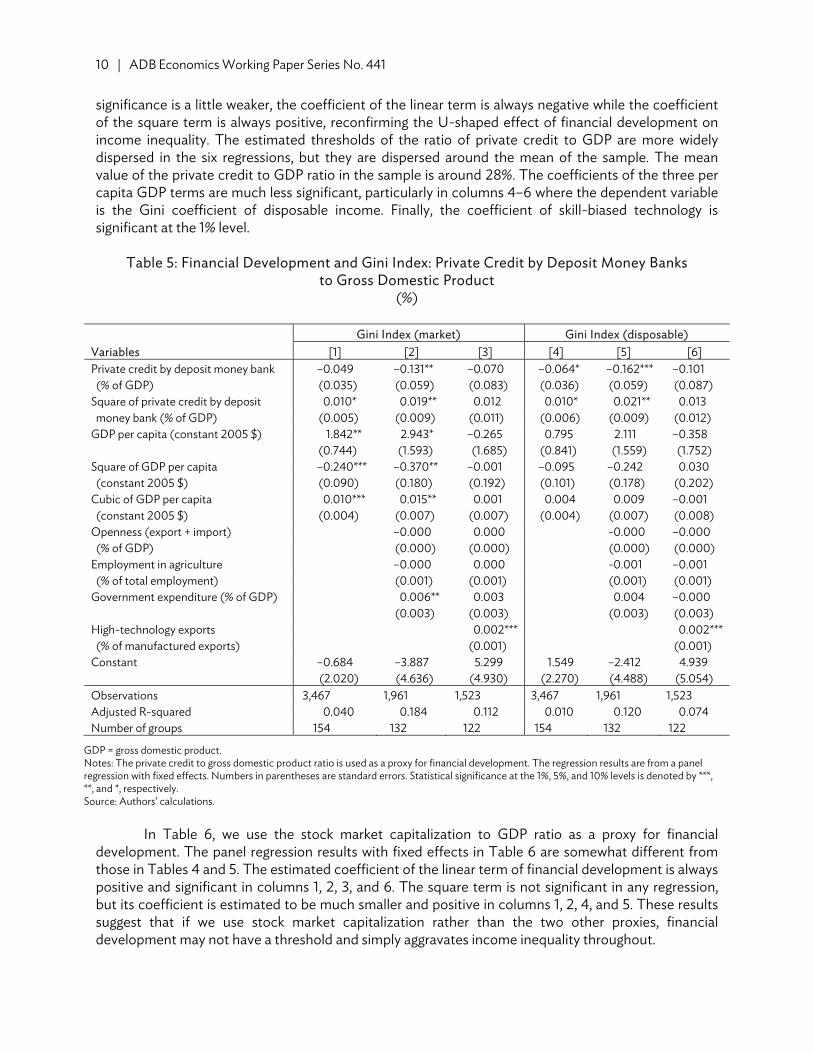
significance is a little weaker, the coefficient of the linear term is always negative while the coefficient of the square term is always positive, reconfirming the U-shaped effect of financial development on income inequality. The estimated thresholds of the ratio of private credit to GDP are more widely dispersed in the six regressions, but they are dispersed around the mean of the sample. The mean value of the private credit to GDP ratio in the sample is around 28%. The coefficients of the three per capita GDP terms are much less significant, particularly in columns 4–6 where the dependent variable is the Gini coefficient of disposable income. Finally, the coefficient of skill-biased technology is significant at the 1% level.

Table 5: Financial Development and Gini Index: Private Credit by Deposit Money Banks


Gini Index (market) Gini Index (disposable)

Variables [1] [2] [3] [4] [5] [6] Private credit by deposit money bank –0.049 –0.131** –0.070 –0.064* –0.162*** –0.101 (% of GDP) (0.035) (0.059) (0.083) (0.036) (0.059) (0.087) Square of private credit by deposit 0.010* 0.019** 0.012 0.010* 0.021** 0.013 money bank (% of GDP) (0.005) (0.009) (0.011) (0.006) (0.009) (0.012) GDP per capita (constant 2005 $) 1.842** 2.943* –0.265 0.795 2.111 –0.358

(0.744) (1.593) (1.685) (0.841) (1.559) (1.752) Square of GDP per capita –0.240*** –0.370** –0.001 –0.095 –0.242 0.030 (constant 2005 $) (0.090) (0.180) (0.192) (0.101) (0.178) (0.202) Cubic of GDP per capita 0.010*** 0.015** 0.001 0.004 0.009 –0.001 (constant 2005 $) (0.004) (0.007) (0.007) (0.004) (0.007) (0.008) Openness (export + import) –0.000 0.000 -0.000 –0.000 (% of GDP) (0.000) (0.000) (0.000) (0.000) Employment in agriculture –0.000 0.000 -0.001 –0.001 (% of total employment) (0.001) (0.001) (0.001) (0.001) Government expenditure (% of GDP) 0.006** 0.003 0.004 –0.000

(0.003) (0.003) (0.003) (0.003) High-technology exports 0.002*** 0.002*** (% of manufactured exports) (0.001) (0.001) Constant –0.684 –3.887 5.299 1.549 –2.412 4.939 (2.020) (4.636) (4.930) (2.270) (4.488) (5.054) Observations 3,467 1,961 1,523 3,467 1,961 1,523 Adjusted R-squared 0.040 0.184 0.112 0.010 0.120 0.074 Number of groups 154 132 122 154 132 122

GDP = gross domestic product. Notes: The private credit to gross domestic product ratio is used as a proxy for financial development. The regression results are from a panel regression with fixed effects. Numbers in parentheses are standard errors. Statistical significance at the 1%, 5%, and 10% levels is denoted by ***, **, and *, respectively. Source: Authors’ calculations.

In Table 6, we use the stock market capitalization to GDP ratio as a proxy for financial

development. The panel regression results with fixed effects in Table 6 are somewhat different from those in Tables 4 and 5. The estimated coefficient of the linear term of financial development is always positive and significant in columns 1, 2, 3, and 6. The square term is not significant in any regression, but its coefficient is estimated to be much smaller and positive in columns 1, 2, 4, and 5. These results suggest that if we use stock market capitalization rather than the two other proxies, financial development may not have a threshold and simply aggravates income inequality throughout.


Table 6: Financial Development and Gini Index: Stock Market Capitalization


Gini Index (market) Gini Index (disposable)

Variables [1] [2] [3] [4] [5] [6] Stock market capitalization 0.014* 0.011** 0.020** 0.009 0.009 0.025** (% of GDP) (0.007) (0.005) (0.008) (0.007) (0.007) (0.011) Square of stock market capitalization 0.000 0.001 -0.001 0.000 0.001 –0.002 (% of GDP) (0.001) (0.001) (0.002) (0.001) (0.001) (0.002) GDP per capita (constant 2005 $) 1.446 2.563 1.970 0.773 2.901** 2.839*

(1.311) (1.614) (1.685) (1.331) (1.333) (1.480) Square of GDP per capita –0.205 –0.328* –0.260 –0.109 -0.345** –0.342* (constant 2005 $) (0.152) (0.182) (0.189) (0.152) (0.154) (0.173)

Gini Index (market) Gini Index (disposable) Variables [1] [2] [3] [4] [5] [6] Cubic of GDP per capita 0.009 0.014** 0.011 0.005 0.014** 0.014** (constant 2005 $) (0.006) (0.007) (0.007) (0.006) (0.006) (0.007) Openness (export + import) 0.000 0.000 0.000 –0.000 (% of GDP) (0.000) (0.000) (0.000) (0.000) Employment in agriculture -0.000 -0.000 -0.001 -0.001 (% of total employment) (0.001) (0.001) (0.001) (0.001) Government expenditure (% of GDP) 0.002 0.002 –0.001 –0.002

(0.002) (0.002) (0.002) (0.003) High-technology exports 0.001 0.001** (% of manufactured exports) (0.001) (0.001) Constant 0.515 –2.829 –1.131 1.721 –4.546 –4.297 (3.715) (4.731) (4.974) (3.810) (3.747) (4.137) Observations 1,734 1,414 1,341 1,734 1,414 1,341 Adjusted R-squared 0.078 0.111 0.084 0.046 0.088 0.092 Number of groups 102 96 93 102 96 93

GDP = gross domestic product. Notes: The stock market capitalization to gross domestic product ratio is used as a proxy for financial development. The regression results are from a panel regression with fixed effects. Numbers in parentheses are standard errors. Statistical significance at the 1%, 5%, and 10% levels is denoted by ***, **, and *, respectively. Source: Authors’ calculations.

In Table 7, we used the top 1% income share as a dependent variable. The proxy for financial

development is the liquid liabilities to GDP ratio in columns 1–3, the private credit to GDP ratio in columns 4–6, and the stock market capitalization to GDP ratio in columns 7–9.

The results in Table 7 are broadly similar to those in Tables 4–6. Again, if the liquid liabilities to

GDP ratio or the private credit to GDP ratio is used as the proxy for financial development, the estimated coefficient of the linear term is always negative and the estimated coefficient of the square term is always positive, suggesting a U-shaped effect. However, the statistical significance is lower than that in Tables 4 and 5. If the stock market capitalization to GDP ratio is used as the proxy, the estimated coefficient of the linear term is positive and significant at 1%. The square term is insignificant suggesting that stock market development aggravates income inequality throughout.


Table 7: Financial Development and Top 1% Income Share

Income Share (top 1%)Variables [1] [2] [3] [4] [5] [6] [7] [8] [9]Liquid liabilities (% of GDP) –0.116 –0.187 –0.186

(0.102) (0.136) (0.186) Square of Liquid liabilities (% of GDP) 0.015 0.019 0.023

(0.017) (0.021) (0.024) Private credit by deposit money bank –0.073 –0.156* –0.052 (% of GDP) (0.056) (0.086) (0.110)Square of private credit by deposit money bank 0.013 0.021 0.003 (% of GDP) (0.010) (0.013) (0.016)Stock market capitalization (% of GDP) 0.037*** 0.037*** 0.022

(0.012) (0.011) (0.020)Square of stock market capitalization –0.002 –0.003 –0.002 (% of GDP) (0.003) (0.003) (0.004)GDP per capita (constant 2005 $) 2.589* 4.031 0.605 2.798* 4.636* 1.781 2.415 2.497 3.737

(1.415) (2.797) (3.171) (1.425) (2.623) (3.035) (2.007) (2.907) (2.938)Square of GDP per capita (constant 2005 $) –0.329* –0.506 –0.129 –0.353** –0.573* –0.269 –0.320 –0.330 –0.479

(0.176) (0.331) (0.366) (0.177) (0.314) (0.358) (0.241) (0.334) (0.339)Cubic of GDP per capita (constant 2005 $) 0.014* 0.022* 0.008 0.015** 0.024* 0.014 0.015 0.015 0.021

(0.007) (0.013) (0.014) (0.007) (0.012) (0.014) (0.009) (0.013) (0.013)Openness (export + import) (% of GDP) –0.000 0.000 –0.000 0.000 –0.000 0.000

(0.001) (0.001) (0.001) (0.001) (0.001) (0.001)Employment in agriculture –0.003 –0.003* –0.002 –0.003* –0.003** –0.003** (% of total employment) (0.002) (0.002) (0.002) (0.002) (0.001) (0.001)Government expenditure (% of GDP) 0.006 0.004 0.007 0.008* 0.004 0.003

(0.005) (0.004) (0.004) (0.004) (0.004) (0.004)High-technology exports 0.002* 0.002** 0.002 (% of manufactured exports) (0.001) (0.001) (0.001)Constant –4.457 –8.816 1.354 –5.087 –10.650 –2.141 –4.545 –4.820 –8.182 (3.718) (7.762) (9.065) (3.764) (7.174) (8.554) (5.502) (8.398) (8.432)Observations 3,475 1,961 1,524 3,467 1,961 1,523 1,734 1,414 1,341Adjusted R-squared 0.039 0.223 0.241 0.040 0.221 0.235 0.176 0.241 0.252Number of groups 153 131 121 154 132 122 102 96 93

GDP = gross domestic product. Notes: The proxy for financial development is the liquid liabilities to GDP ratio in columns 1-3, the private credit to GDP ratio in columns 4–6 and the stock market capitalization to GDP ratio in columns 7–9. The regression results are from a panel regression with fixed effects. Numbers in parentheses are standard errors. Statistical significance at the 1%, 5%, and 10% levels is denoted by ***, **, and * respectively. Source: Authors’ calculations.


IV. FINANCIAL DEVELOPMENT AND INCOME INEQUALITY: CAUSALITY AND DETERMINANTS

While the results in Tables 4–7 are suggestive, they do not prove a causal relation running from financial development to income inequality; it is important to do so because there are some grounds for causality. For example, as inequality increases, the rich may accumulate more capital and demand more financial services in order to earn higher returns. Or, as inequality decreases, the poor may earn higher incomes and start to save more and open bank accounts. Therefore, in order to establish causality more clearly, we performed two additional analyses. The first is to use instrumental variables estimation. The second is to change the regression into a growth form.

A number of studies have used various variables as instrumental variables for financial development. For example, Beck, Demirgüç-Kunt, and Levine (2003) used legal origins and latitude as instrumental variables for financial development. Since financial transactions are based on contracts, La Porta et al. (1998) argued that legal origins, which produce and enforce laws to better protect the rights of investors, are more conducive for financial development. According to Acemoglu, Johnson, and Robinson (2001), natural resource endowments for which latitude is used as a rough proxy help explain the development of institutions related to finance.

Since our regressions are based on a panel regression with fixed effects, we could not use

either legal origins or latitude which are not time varying as an instrumental variable. Instead, we used law and order data collected from the International Country Risk Guide (ICRG). ICRG assesses law and order separately; each is scored from 0 to 3 points. Law captures the strength and impartiality of the legal system while order reflects popular observance of the law. Since law and order is used as an instrumental variable for both the linear and square terms of financial development, we relied on the control function approach. The basic idea of the method is to derive the residual by regressing endogenous variables on the instrumental variable so that, conditional on the residual, the endogeneity problem disappears.8

The panel instrumental variable estimation results are reported in Table 8. The dependent

variable is the Gini coefficient of market income.9 The proxy for financial development is the liquid liabilities to GDP ratio in columns 1–3, the private credit to GDP ratio in columns 4–6, and the stock market capitalization to GDP ratio in columns 7–9.

Again, if the liquid liabilities to GDP ratio or the private credit to GDP ratio is used as the proxy

for financial development, the estimated coefficient of the linear term is negative and the estimated coefficient of the square term is positive except in column 6, suggesting a U-shaped effect. The estimated coefficient of the square term is significant either at the 1% or 5% level except for column 6. Hence the instrumental variable estimation preserves our main results.

The coefficient of skill-biased technology is significant at either the 1% or the 10% level. A high

share of agriculture in employment is significant at the 5% level in columns 3 and 6. Interestingly, the share of government expenditure in GDP is positive and mostly significant, suggesting that large government expenditures increase income inequality.

8 See Wooldridge (2010) for a detailed explanation for the control function approach. 9 As shown in Section II, there is a possibility that the Gini coefficient based on disposable income is influenced significantly

by different taxation and transfer policies. Therefore, we instead use the Gini coefficient based on market income.


Table 8: Financial Development and Gini Index of Market Income (IV Regression)

Variables Gini Index (market)

[1] [2] [3] [4] [5] [6] [7] [8] [9]Liquid liabilities (% of GDP) –0.231*** –0.217** –0.214**

(0.075) (0.091) (0.103)Square of Liquid liabilities (% of GDP) 0.035*** 0.031*** 0.036***

(0.005) (0.006) (0.007)Private credit by deposit money bank –0.048 –0.042 0.025 (% of GDP) (0.029) (0.038) (0.041)Square of private credit by deposit money 0.007*** 0.007** -0.002 bank (% of GDP) (0.002) (0.003) (0.004)Stock market capitalization (% of GDP) 0.250*** 0.122 0.110

(0.085) (0.094) (0.103) Square of stock market capitalization 0.002** 0.001 -0.000 (% of GDP) (0.001) (0.001) (0.001) GDP per capita (constant 2005 $) 0.857*** 3.049*** 0.624 1.120*** 3.590*** 1.314** 1.797*** 2.863*** 2.262***

(0.298) (0.441) (0.551) (0.297) (0.431) (0.539) (0.402) (0.527) (0.557) Square of GDP per capita –0.124*** –0.372*** –0.094 –0.159*** –0.437*** –0.184*** –0.249*** –0.367*** –0.297*** (constant 2005 $) (0.036) (0.052) (0.065) (0.036) (0.051) (0.064) (0.048) (0.061) (0.065) Cubic of GDP per capita 0.006*** 0.015*** 0.004* 0.007*** 0.018*** 0.008*** 0.011*** 0.015*** 0.012*** (constant 2005 $) (0.001) (0.002) (0.002) (0.001) (0.002) (0.002) (0.002) (0.002) (0.003) Openness (export + import) (% of GDP) –0.000 –0.000 0.000 0.000 0.000** 0.000

(0.000) (0.000) (0.000) (0.000) (0.000) (0.000) Employment in agriculture 0.001 0.001** 0.000 0.001** –0.000 –0.000 (% of total employment) (0.000) (0.000) (0.000) (0.000) (0.000) (0.000) Government expenditure (% of GDP) 0.004*** 0.001 0.005*** 0.003** 0.003** 0.003**

(0.001) (0.001) (0.001) (0.001) (0.001) (0.001) High-technology exports 0.001*** 0.001*** 0.001* (% of manufactured exports) (0.000) (0.000) (0.000) Constant 2.146*** –4.344*** 2.696* 1.253 –6.082*** 0.676 –1.122 –3.906*** –2.134 (0.808) (1.249) (1.572) (0.789) (1.189) (1.501) (1.118) (1.491) (1.577) Observations 2,318 1,654 1,374 2,319 1,656 1,376 1,538 1,292 1,234Number of groups 121 113 107 122 114 108 92 88 87Adjusted R-squared 0.051 0.108 0.025 0.035 0.104 0.019 0.049 0.067 0.029

GDP = gross domestic product. Notes: The proxy for financial development is the liquid liabilities to gross domestic product (GDP) ratio in columns 1–3, the private credit to GDP ratio in columns 4–6 and the stock market capitalization to GDP ratio in columns 7–9. The regression results are from a panel instrumental variable regression with fixed effects. Numbers in parentheses are standard errors. Statistical significance at the 1%, 5%, and 10% levels is denoted by ***, **, and * respectively. Source: Authors’ calculations.


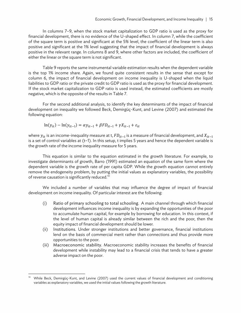
In columns 7–9, when the stock market capitalization to GDP ratio is used as the proxy for financial development, there is no evidence of the U-shaped effect. In column 7, while the coefficient of the square term is positive and significant at the 5% level, the coefficient of the linear term is also positive and significant at the 1% level suggesting that the impact of financial development is always positive in the relevant range. In columns 8 and 9, where other factors are included, the coefficient of either the linear or the square term is not significant.

Table 9 reports the same instrumental variable estimation results when the dependent variable

is the top 1% income share. Again, we found quite consistent results in the sense that except for column 6, the impact of financial development on income inequality is U-shaped when the liquid liabilities to GDP ratio or the private credit to GDP ratio is used as the proxy for financial development. If the stock market capitalization to GDP ratio is used instead, the estimated coefficients are mostly negative, which is the opposite of the results in Table 7.

For the second additional analysis, to identify the key determinants of the impact of financial

development on inequality we followed Beck, Demirgüç-Kunt, and Levine (2007) and estimated the following equation:

ln ln

where is an income-inequality measure at t, is a measure of financial development, and is a set of control variables at (t–1). In this setup, t implies 5 years and hence the dependent variable is the growth rate of the income inequality measure for 5 years.

This equation is similar to the equation estimated in the growth literature. For example, to investigate determinants of growth, Barro (1991) estimated an equation of the same form where the dependent variable is the growth rate of per capita GDP. While the growth equation cannot entirely remove the endogeneity problem, by putting the initial values as explanatory variables, the possibility of reverse causation is significantly reduced.10

We included a number of variables that may influence the degree of impact of financial

development on income inequality. Of particular interest are the following: (i) Ratio of primary schooling to total schooling. A main channel through which financial

development influences income inequality is by expanding the opportunities of the poor to accumulate human capital, for example by borrowing for education. In this context, if the level of human capital is already similar between the rich and the poor, then the equity impact of financial development should be lower.

(ii) Institutions. Under stronger institutions and better governance, financial institutions lend on the basis of commercial merit rather than connections and thus provide more opportunities to the poor.

(iii) Macroeconomic stability. Macroeconomic stability increases the benefits of financial development while instability may lead to a financial crisis that tends to have a greater adverse impact on the poor.

10 While Beck, Demirgüç-Kunt, and Levine (2007) used the current values of financial development and conditioning

variables as explanatory variables, we used the initial values following the growth literature.


Table 9: Financial Development and Top 1% Income Share (IV Regression)

Income Share (top 1%)Variables [1] [2] [3] [4] [5] [6] [7] [8] [9]Liquid liabilities (% of GDP) –0.717*** –0.663*** –0.359*

(0.142) (0.178) (0.194) Square of Liquid liabilities (% of GDP) 0.030*** 0.012 0.009

(0.009) (0.011) (0.014) Private credit by deposit money bank –0.248*** –0.211*** 0.077 (% of GDP) (0.056) (0.074) (0.078)Square of private credit by deposit 0.008* 0.002 –0.024*** money bank (% of GDP) (0.004) (0.006) (0.007)Stock market capitalization (% of GDP) –0.058 –0.319* –0.266

(0.173) (0.180) (0.196)Square of stock market capitalization –0.001 –0.003* –0.003 (% of GDP) (0.002) (0.002) (0.002)GDP per capita (constant 2005 $) –0.072 2.442*** 2.436** 0.306 2.987*** 4.012*** 2.388*** 2.969*** 4.287***

(0.564) (0.857) (1.038) (0.564) (0.843) (1.018) (0.820) (1.009) (1.062)Square of GDP per capita –0.021 –0.309*** –0.335*** –0.069 –0.378*** –0.541*** –0.320*** –0.391*** –.550*** (constant 2005 $) (0.069) (0.101) (0.122) (0.069) (0.100) (0.120) (0.098) (0.117) (0.124)Cubic of GDP per capita 0.003 0.014*** 0.016*** 0.005* 0.017*** 0.025*** 0.015*** 0.018*** 0.024*** (constant 2005 $) (0.003) (0.004) (0.005) (0.003) (0.004) (0.005) (0.004) (0.004) (0.005)Openness (export + import) –0.000 0.000 0.000 0.000 0.000 0.000 (% of GDP) (0.000) (0.000) (0.000) (0.000) (0.000) (0.000)Employment in agriculture –0.002** –0.002*** –0.002*** –0.002*** –0.003*** –0.003*** (% of total employment) (0.001) (0.001) (0.001) (0.001) (0.001) (0.001)Government expenditure (% of GDP) 0.006*** 0.004* 0.006*** 0.008*** 0.007*** 0.005**

(0.002) (0.002) (0.002) (0.002) (0.002) (0.002)High-technology exports 0.002*** 0.002*** 0.002** (% of manufactured exports) (0.001) (0.001) (0.001)Constant 4.421*** –2.822 –3.115 2.022 –5.758** -8.211*** –4.102* –4.794* –8.562*** (1.529) (2.429) (2.962) (1.496) (2.325) (2.833) (2.282) (2.856) (3.006)Observations 2,318 1,654 1,374 2,319 1,656 1,376 1,538 1,292 1,234Adjusted R-squared 0.126 0.194 0.196 0.113 0.184 0.200 0.136 0.197 0.203Number of groups 121 113 107 122 114 108 92 88 87

GDP = gross domestic product. Notes: The proxy for financial development is the liquid liabilities to gross domestic product ratio in columns 1–3, the private credit to GDP ratio in columns 4–6 and the stock market capitalization to GDP ratio in columns 7–9. The regression results are from a panel instrumental variable regression with fixed effects. Numbers in parentheses are standard errors. Statistical significance at the 1%, 5%, and 10% levels is denoted by ***, **, and * respectively. Source: Authors’ calculations.


To get the ratio of primary schooling, we divided average years of primary schooling by average

years of total schooling collected from Barro and Lee (2013). While this ratio does not directly capture the education gap between the rich and the poor, a high ratio implies there is more scope for additional education for less educated people who are more likely to be poor. The quality of institutions was measured by law and order. Finally, macroeconomic stability was measured by the inflation rate from t–1 to t.

The Gini coefficient of market income is used to measure income inequality. We estimated a

panel regression with fixed effects and report the results in Table 10. The liquid liabilities to GDP ratio is used as the proxy for financial development. We used the initial per capita GDP, trade openness, government expenditure share in GDP, share of high-technology exports, and the employment share of agriculture as control variables.

While not reported, the linear and square terms of the liquid liabilities to GDP ratio were

mostly insignificant if their interaction terms were not included; however, the interactions of the linear term with factors that were expected to influence the degree of impact of financial development on income inequality were generally significant; we report only those results.

We found that the coefficients of interaction terms had the right signs and were mostly

significant. The interaction term with the ratio of primary schooling was negative indicating that financial development has a stronger pro-equity impact when the ratio of primary schooling is higher. The interaction term with law and order was statistically significant at 10% only in column 6, but it is negative providing some support for the notion that the pro-equity effect of financial development becomes stronger when law and order improves.

Macroeconomic stability does not, however, seem to strengthen the pro-equity effect of

financial development. While significant at the 10% level only in column 9, the interaction term with the inflation rate is negative. This result implies that while macroeconomic stability may increase the benefits of financial development, reduced income inequality is not one of those benefits.

The results in Table 11 where the private credit to GDP ratio is the proxy for financial

development are generally consistent with those in Table 10. The interaction terms with the ratio of primary schooling as well as law and order are all negative. The interaction term with the ratio of primary schooling was somewhat less significant than in Table 10, but it is significant at either 5% or 10% in columns 1 and 2. The interaction term with law and order was more significant at 5% in column 6. Again, these results suggest that when the ratio of primary schooling increases or when law and order improves, financial development becomes more effective in reducing income inequality though again, we did not find a similar pro-equity effect for macroeconomic stability.

Finally, in Table 12 we report the results when the stock market capitalization to GDP ratio is

used as the proxy for financial development. We did not find any effect for the ratio of primary schooling or law and order. All the coefficients of the interaction terms were insignificant. Interestingly, however, the interaction term with the inflation rate was positive and significant in column 7 at the 10% level and in column 9 at the 1% level. This result suggests that as macroeconomic stability improves (inflation decreases), financial development measured by stock market capitalization becomes more effective in reducing income inequality.


Table10: Factors that Influence the Degree of Impact of Financial Development on Market Income Inequality: Liquid Liabilities to Gross Domestic Product

(%)

Growth of Gini Coefficient (market) Variables [1] [2] [3] [4] [5] [6] [7] [8] [9] Log of initial Gini index (market) –0.102*** –0.102*** –0.176*** –0.138*** –0.144*** -0.162*** –0.102*** –0.103*** –0.165*** (0.008) (0.008) (0.016) (0.012) (0.011) (0.021) (0.009) (0.009) (0.022) Initial liquid liabilities (% of GDP) 0.017*** 0.011 0.028 0.000 –0.002 –0.010 0.001 –0.001 –0.013*

(0.006) (0.007) (0.027) (0.003) (0.003) (0.007) (0.003) (0.003) (0.007) Initial liquid liabilities –0.024*** –0.017** –0.069* × Ratio of primary schooling (0.007) (0.008) (0.039) Initial liquid liabilities 0.001 –0.013 –0.149* × Law and Order (0.004) (0.042) (0.079) Initial liquid liabilities –0.002 –0.002* –0.008 × Growth of consumer price index (0.001) (0.001) (0.006) Initial human capital –0.047*** –0.045** –0.181** 0.001 –0.009 –0.100** –0.006 –0.025* –0.087* (0.018) (0.018) (0.072) (0.017) (0.022) (0.045) (0.012) (0.013) (0.044) Initial GDP per capita 0.007 0.024 0.014** 0.041*** 0.011*** 0.036*** (constant 2005 $) (0.004) (0.014) (0.006) (0.012) (0.004) (0.012) Log of openness (exports + imports) –0.003 -0.006 –0.011** –0.010 –0.004 –0.011 (% of GDP) (0.004) (0.009) (0.005) (0.009) (0.004) (0.009) Average government expenditure 0.001 -0.000 0.001** 0.000 0.001** 0.000 (% of GDP) (0.000) (0.001) (0.000) (0.001) (0.000) (0.001) Log of high-technology exports -0.002 –0.005 –0.003 (% of manufactured exports) (0.002) (0.003) (0.002) Agriculture employment share –0.040** –0.047*** –0.043** (% of total employment) (0.017) (0.018) (0.019) Constant 0.407*** 0.357*** 0.671*** 0.522*** 0.471*** 0.442*** 0.385*** 0.319*** 0.468*** (0.035) (0.048) (0.136) (0.044) (0.062) (0.113) (0.036) (0.044) (0.116) Observations 631 625 233 435 434 226 622 617 231 Number of groups 113 113 82 99 99 79 112 112 81 Adjusted R-squared 0.299 0.306 0.549 0.439 0.459 0.513 0.287 0.305 0.524

GDP = gross domestic product. Notes: The proxy for financial development is the liquid liabilities to gross domestic product ratio. The regression results are from a panel regression with fixed effects. Numbers in parentheses are standard errors. Statistical significance at the 1%, 5%, and 10% levels is denoted by ***, **, and * respectively. Source: Authors’ calculations.


Table 11: Factors that Influence the Degree of Impact of Financial Development on Market Income Inequality: Private Credit by Deposit Money Banks to Gross Domestic Product

(%)

Variables Growth of Gini Coefficient (market)

[1] [2] [3] [4] [5] [6] [7] [8] [9] Log of initial Gini index (market) –0.103*** –0.104*** –0.173*** –0.142*** –0.145*** –0.171*** –0.104*** –0.105*** –0.170*** (0.009) (0.009) (0.019) (0.011) (0.011) (0.019) (0.009) (0.009) (0.020) Initial private credit by deposit money 0.017*** 0.016** 0.015 0.007** 0.006* 0.009 0.005** 0.005* 0.003 bank (% of GDP) (0.005) (0.006) (0.019) (0.003) (0.003) (0.006) (0.002) (0.003) (0.006) Initial private credit by deposit money –0.020** –0.017* –0.024 bank × Ratio of primary schooling (0.008) (0.009) (0.025) Initial private credit by deposit money –0.017 –0.026 –0.145** bank × Law and order (0.045) (0.046) (0.070) Initial private credit by deposit money –0.002 –0.002 –0.009 bank × Growth of consumer price index (0.002) (0.002) (0.011) Initial human capital –0.048*** –0.043*** –0.110** –0.010 –0.008 –0.090** –0.020* –0.026** –0.077* (0.017) (0.016) (0.053) (0.017) (0.020) (0.042) (0.012) (0.013) (0.040) Initial GDP per capita (constant 2005 $) 0.001 0.017 0.007 0.019 0.005 0.018

(0.005) (0.017) (0.006) (0.015) (0.004) (0.013) Log of openness (exports + imports) –0.003 –0.010 –0.012** –0.010 –0.004 –0.011 (% of GDP) (0.004) (0.009) (0.005) (0.009) (0.004) (0.009) Average government expenditure 0.001 0.000 0.001* 0.000 0.001* 0.000 (% of GDP) (0.000) (0.001) (0.000) (0.001) (0.000) (0.001) Log of high-technology exports -0.002 –0.004 –0.003 (% of manufactured exports) (0.002) (0.003) (0.002) Agriculture employment share –0.033* –0.039** –0.035 (% of total employment) (0.020) (0.019) (0.021) Constant 0.403*** 0.394*** 0.619*** 0.523*** 0.515*** 0.577*** 0.387*** 0.359*** 0.576*** (0.034) (0.058) (0.144) (0.043) (0.063) (0.113) (0.036) (0.052) (0.100) Observations 631 625 237 437 436 230 622 617 235 Number of groups 115 115 84 101 101 81 114 114 83 Adjusted R-squared 0.303 0.309 0.500 0.449 0.462 0.497 0.297 0.307 0.502

GDP = gross domestic product. Notes: The proxy for financial development is the private credit to gross domestic product ratio. The regression results are from a panel regression with fixed effects. Numbers in parentheses are standard errors. Statistical significance at the 1%, 5%, and 10% levels is denoted by ***, **, and * respectively. Source: Authors’ calculations.


Table 12: Factors that Influence the Degree of Impact of Financial Development on Market Income Inequality: Stock Market Capitalization to Gross Domestic Product

(%)

Variables Growth of Gini Coefficient (market)

[1] [2] [3] [4] [5] [6] [7] [8] [9] Log of initial Gini index (market) –0.184*** –0.181*** –0.182*** –0.179*** –0.179*** –0.177*** –0.180*** –0.179*** –0.181***

(0.015) (0.016) (0.022) (0.018) (0.018) (0.024) (0.017) (0.018) (0.024) Initial stock market capitalization 0.013 0.007 0.009 0.003 0.003 0.006 0.001 –0.000 –0.001 (% of GDP) (0.012) (0.014) (0.017) (0.004) (0.004) (0.005) (0.002) (0.002) (0.002) Initial stock market capitalization –0.017 –0.010 –0.010 x Ratio of primary schooling (0.020) (0.022) (0.028) Initial stock market capitalization –0.009 –0.043 –0.080 x Average law and order (0.077) (0.077) (0.087) Initial stock market capitalization 0.011* 0.010 0.021*** x Growth of consumer price index (0.006) (0.007) (0.008) Initial human capital –0.079 –0.097** –0.099 –0.057 –0.095** –0.092* –0.032 –0.069* –0.067 (0.050) (0.045) (0.066) (0.038) (0.040) (0.049) (0.036) (0.038) (0.045) Initial GDP per capita 0.023** 0.020 0.024** 0.020 0.023** 0.023* (constant 2005 $) (0.012) (0.013) (0.010) (0.012) (0.009) (0.012) Log of openness (exports + imports) –0.008 –0.013 –0.007 –0.010 –0.006 –0.008 (% of GDP) (0.008) (0.011) (0.008) (0.011) (0.008) (0.011) Average government expenditure 0.000 0.001 0.001 0.001 0.001 0.001 (% of GDP) (0.001) (0.001) (0.001) (0.001) (0.001) (0.001) Log of high-technology exports –0.002 –0.005 –0.002 (% of manufactured exports) (0.003) (0.004) (0.003) Agriculture employment share –0.037 –0.049* –0.030 (% of total employment) (0.027) (0.027) (0.025) Constant 0.739*** 0.567*** 0.615*** 0.708*** 0.540*** 0.589*** 0.693*** 0.535*** 0.542*** (0.059) (0.123) (0.135) (0.068) (0.101) (0.135) (0.062) (0.094) (0.137) Observations 260 260 210 246 246 205 257 257 208 Number of groups 87 87 75 81 81 73 86 86 74 Adjusted R-squared 0.480 0.491 0.475 0.476 0.488 0.476 0.483 0.495 0.491

GDP = gross domestic product. Notes: The proxy for financial development is the stock market capitalization to GDP ratio. The regression results are from a panel regression with fixed effects. Numbers in parentheses are standard errors. Statistical significance at the 1%, 5%, and 10% levels is denoted by ***, **, and * respectively. Source: Authors’ calculations.

V. CONCLUDING REMARKS

In this paper we empirically examine the impact of financial development on income inequality. This issue is of more than passing interest for developing Asia since it intersects two significant strategic challenges facing the region in the 21st century: fostering a more efficient financial system and tackling growing inequality. Conceptually, the direction of the finance-inequality nexus is ambiguous. On the one hand there are grounds for a pro-equity impact of financial development. More specifically, financial development can improve the access of the poor to financial services enabling them to become more productive, for example by opening up new businesses. On the other hand, financial development may increase inequality if it takes the form of more and better financial services for the better off and delivers higher returns to their capital without significant improvement in access for the poor thus widening the gap between the rich and the poor. Therefore, the impact of financial development on income inequality is ultimately an empirical issue.

In light of the extensive literature on the relationship between per capita income and income inequality starting with the seminal work of Kuznets, we included per capita income as an important additional variable. In the context of the income-inequality nexus, we found an inverted U-shaped relationship between per capita income and income inequality up to a certain level of per capita income in line with the Kuznets curve. As income continues to increase, however, income inequality starts to increase again. This is consistent with the stylized facts, in particular the growing inequality in the US and other advanced economies in recent years. This finding holds for both measures of inequality, i.e. the Gini coefficient and the top 1% income share.

The analysis of our central issue—the relationship between financial development and income

inequality—yields a number of significant and interesting findings. Above all, we found evidence of a U-shaped relationship between financial development and income inequality. As the financial system develops, inequality improves until it reaches approximately the mean level, but as the financial system continues to develop, it aggravates income inequality. Our evidence points to the possibility that increased income inequality in advanced countries is related to the adverse impact of financial development on income inequality. To test the robustness of our results, we performed two additional analyses—an instrumental variables estimation and a growth form regression—to address possible endogeneity issues. By and large, the results of both analyses are consistent with earlier results.

With respect to our central issue, an interesting and natural follow-up question is: What are

the factors that influence the degree of the impact? That is, what are the factors that determine whether or not financial development will have a significant effect on income inequality? We looked at three factors for which there are conceptual grounds for an effect on the finance-inequality nexus: the ratio of primary schooling to total schooling, law and order, and macroeconomic stability. As expected, our evidence indicates that when the ratio of primary schooling increases and law and order improves, financial development is more effective in reducing inequality. Our results thus suggest that financial development can help reduce inequality by enabling the poor to finance their educations and human capital investments. On the other hand, macroeconomic stability did not affect the relationship.

Overall, our findings imply that the effect of financial development on income inequality is

mixed and inconclusive. Therefore, our empirical evidence mirrors the conceptual ambiguity noted earlier. There are grounds for both a beneficial and a harmful effect of financial development on inequality. In addition, our finding of a U-shaped relationship between finance and inequality echoes the finding of a U-shaped relationship between finance and growth by a number of earlier studies. Taken together, the two U-shaped relationships suggest that financially less-developed economies


stand to reap the largest growth and equity gains from financial development. They also lend some support to the popular notion that financially advanced countries have too much finance, since finance may contribute to neither growth nor equity in those countries.

The salient policy implication of our empirical evidence is that financial development per se

does not automatically reduce income inequality. Intuitively, reduced inequality is more likely the product of financial inclusion than of financial development. Therefore, it would be worthwhile to include financial inclusion as an additional independent variable in the empirical analysis if only the data were available. There is, however, a negative correlation between the Gini coefficient and financial inclusion which supports the conjecture (Figure 3). Financial development must be accompanied by financial inclusion to foster inclusive growth.

Figure 3: Income Inequality and Financial Inclusion, 2011

Notes: The fitted line is derived from a regression equation where the Gini index is the dependent variable and loans from a financial institution to the bottom 40% of the population as the explanatory variable. Data refer to 65 economies. Source: Authors’ calculations based on data from the Standardized World Income Inequality Database (SWIID) (Solt 2014) and Demirgüç-Kunt and Klapper (2013).

y = -0.3635x + 39.264[0.1696] [1.8424]

0

10

20

30

40

50

60

0 5 10 15 20 25 30 35

Gin

i inde

x of i

nequ

ality

in e

quiv

alize

d ho

useh

old

disp

osab

le in

com

e

Loan from a financial institution in the past year, income, bottom 40% (% age 15+), 2011

REFERENCES Acemoglu, D., S. Johnson, and J. A. Robinson. 2001. The Colonial Origins of Comparative

Development: An Empirical Investigation. American Economic Review. 91 (5). pp. 1369–1401. Acemoglu, D. and J. A. Robinson. 2002. The Political Economy of the Kuznets Curve. Review of

Development Economics. 6 (2). pp. 183–203. Ahluwalia, M. S. 1976. Inequality, Poverty and Development. Journal of Development Economics. 3 (4).

pp. 307–42. Arcand, J.-L., E. Berkes, and U. Panizza. 2012. Too Much Finance? IMF Working Paper Series. No. 12–

161. Washington, DC: International Monetary Fund. Barro, R. J. 1991. Economic Growth in a Cross Section of Countries. Quarterly Journal of Economics. 106.

(2). pp. 407–43. Barro, R. J. and J.-W. Lee. 2013. A New Data Set of Educational Attainment in the World, 1950–2010.

Journal of Development Economics. 104. pp. 184–98. Beck, T., A. Demirgüç-Kunt, and R. Levine. 2003. Law, Endowments and Finance. Journal of Financial

Economics. 70 (2). pp. 137–81. ————. 2007. Finance, Inequality, and the Poor. Journal of Economic Growth. 12 (1). pp. 27–49. Cecchetti, S. G. and E. Kharroubi. 2012. Reassessing the Impact of Finance on Growth. BIS Working

Papers. No. 381. Frankfurt: Bank for International Settlements. Demirgüç-Kunt, A. and L. Klapper. 2013. Measuring Financial Inclusion: Explaining Variation in Use of

Financial Services across and within Countries. Brookings Papers on Economic Activity. Brookings Institution.

Demirgüç-Kunt, A. and R. Levine. 2009. Finance and Inequality: Theory and Evidence. Annual Review

of Financial Economics. 1 (1). pp. 287–318. Goldin, C. and L. Katz. 2008. The Race between Education and Technology. Cambridge, MA: Harvard

University Press. Horioka, C. and A. Terada-Hagiwara. 2012. The Determinants of Saving Rates in Developing Asia.

Japan and the World Economy. 24 (2). pp. 128–37. International Monetary Fund (IMF). 2007. Globalization and Inequality. World Economic Outlook. pp.

31–65. Washington, DC. Jaumotte, F., S. Lall, and C. Papageorgiou. 2013. Rising Income Inequality: Technology, or Trade and

Financial Globalization? International Monetary Fund Working Paper Series. No. 08/185. Washington, DC: International Monetary Fund.

24 | References

Kuznets, S. 1955. Economic Growth and Income Inequality. American Economic Review. 45 (March). pp. 1–28.

La Porta, R., F. Lopez-de-Silanes, A. Shleifer, and R. W. Vishny. 1998. Law and Finance. Journal of

Political Economy. 106 (6). pp. 1113–55. Organisation for Economic Co-operation and Development (OECD). 2008. Growing Unequal?

Income Distribution in OECD Countries. Paris: OECD Publishing. ————. 2012. Reducing Income Inequality while Boosting Economic Growth: Can It Be Done?

Chapter 5 in Economic Policy Reforms 2012: Going for Growth. Paris: OECD Publishing. Papanek, G. and O. Kyn. 1986. The Effect on Income Distribution of Development, the Growth Rate

and Economic Strategy. Journal of Development Economics. 23 (1). pp. 55–65. Piketty, T. 2014. Capital in the Twenty-First Century. Cambridge, MA: Harvard University Press. Piketty, T. and E. Saez. 2003. Income Inequality in the United States, 1913–1998. Quarterly Journal of

Economics. 118 (1). pp. 1–41. ————. 2006. The Evolution of Top Incomes: A Historical and International Perspective. American

Economic Review, Papers and Proceedings. 96 (2). pp. 200–205. Piketty, T., E. Saez, and S. Stantcheva. 2014. Optimal Taxation of Top Labor Incomes: A Tale of Three

Elasticities. American Economic Journal: Economic Policy. 6 (1). pp. 230–71. Solt, F. 2014. The Standardized World Income Inequality Database (SWIID). http://hdl.handle.net/

1902.1/11992. Frederick Solt [Distributor] V14 [Version]. Stolper, W. F. and P. A. Samuelson. 1941. Protection and Real Wages. Review of Economic Studies. 9 (1).

pp. 58–73. Wooldridge, J. M. 2010. Econometric Analysis of Cross Section and Panel Data. Cambridge, MA: MIT

Press.


AsiAn Development BAnk6 ADB Avenue, Mandaluyong City1550 Metro Manila, Philippineswww.adb.org

Economic Growth, Financial Development, and Income Inequality

The paper finds that financial development contributes to reducing inequality up to a point, but as financial development proceeds further, it contributes to greater inequality. Two factors that can help strengthen the impact of financial development on inequality are primary schooling, and law and order.

About the Asian Development Bank

ADB’s vision is an Asia and Pacific region free of poverty. Its mission is to help its developing member countries reduce poverty and improve the quality of life of their people. Despite the region’s many successes, it remains home to the majority of the world’s poor. ADB is committed to reducing poverty through inclusive economic growth, environmentally sustainable growth, and regional integration.

Based in Manila, ADB is owned by 67 members, including 48 from the region. Its main instruments for helping its developing member countries are policy dialogue, loans, equity investments, guarantees, grants, and technical assistance.

EconomIc Growth, FInAncIAl DEvElopmEnt, AnD IncomE InEquAlItyDonghyun Park and Kwanho Shin

adb economicsworking paper series

no. 441

august 2015

Documents

Economic Growth, Financial Development, and Income Inequality · Economic Growth, Financial Development, and Income ... the early stages of economic development as resources are