Economic Growth, Convergence Clubs, and the Role of Financial Development

Economic Growth, Convergence Clubs, and the Role of Financial DevelopmentAuthor(s): J. C. Berthelemy and A. VaroudakisSource: Oxford Economic Papers, New Series, Vol. 48, No. 2 (Apr., 1996), pp. 300-328Published by: Oxford University PressStable URL: http://www.jstor.org/stable/2663729 .

Accessed: 18/06/2014 21:50

Your use of the JSTOR archive indicates your acceptance of the Terms & Conditions of Use, available at .http://www.jstor.org/page/info/about/policies/terms.jsp

.JSTOR is a not-for-profit service that helps scholars, researchers, and students discover, use, and build upon a wide range ofcontent in a trusted digital archive. We use information technology and tools to increase productivity and facilitate new formsof scholarship. For more information about JSTOR, please contact [email protected].

.

Oxford University Press is collaborating with JSTOR to digitize, preserve and extend access to OxfordEconomic Papers.

http://www.jstor.org

This content downloaded from 194.29.185.145 on Wed, 18 Jun 2014 21:50:06 PMAll use subject to JSTOR Terms and Conditions

http://www.jstor.org/action/showPublisher?publisherCode=oup

http://www.jstor.org/stable/2663729?origin=JSTOR-pdf

http://www.jstor.org/page/info/about/policies/terms.jsp


O.xJord Economic Papers 48 (1996), 300-328

ECONOMIC GROWTH, CONVERGENCE CLUBS, AND THE ROLE OF FINANCIAL

DEVELOPMENT By J. C. BERTHELEMY and A. VAROUDAKIS OECD Development Centre, 94, rue Chardon Lagache,

75775 Paris Cedex 16, France

This paper aims to show and test the existence of a poverty trap linked to the development of the banking sector. Our theoretical model exhibits multiple steady state equilibria due to a reciprocal externality between the banking sector and the real sector. Growth in the real sector causes the financial market to expand, thereby increasing banking competition and efficiency. In return, the development of the banking sector raises the net yield on savings and enhances capital accumulation and growth. The aim of our econometric tests is to check the existence of multiple steady states associated with financial and educational development.

1. Introduction

A NUMBER of recent studies have used endogenous growth theory to show the possibility of a close association between the level of development in the financial sector and growth. The general idea consists in assuming that financial development helps to improve the efficiency of capital allocation. The mechanisms involved rely on the possibility of choosing more productive investments through improved management of liquidity risks (Bencivenga and Smith 1991), by more efficiently diversifying investors' portfolios (Levine 1991, Saint-Paul 1992), or by collecting information on the efficiency of various investment projects and/or investors' abilities (Greenwood and Jovanovic 1990, King and Levine 1993a). This factor is then integrated into an endogenous growth model where any increase in capital productivity has a positive effect on the economy's long-run rate of growth.1

Causality between financial development and growth runs however both ways. We have good reason to believe that causality also runs in the opposite direction from per capita income to the development of financial structures, as has already been mentioned in certain previous studies. The first aim of this study is to make a more in-depth theoretical analysis of the interaction between financial development and real growth.

We study an endogenous growth model in which learning-by-doing externalities in the real sector form the source for long-run growth. The financial sector2 uses real resources, which present an opportunity cost in terms of production.3

] An overview of this theoretical literature has been provided by Pagano (1993). 2 In the present paper the financial sector is confined to the banking system without making any

attempt at analysing the distinct role of the development of stock markets in the growth process. In what follows, the terms 'banking sector' and 'financial sector' are therefore used interchangeably.

3 On this particular point the model bears some resemblance to the way Grossman and Helpman (1991) account for resource competition between the final goods sector and the R&D sector of the economy.

C) Oxford University Press 1996



J. C. BERTHELEMY AND A. VAROUDAKIS 301

By collecting information about investment opportunities it directs savings towards more productive investments, increasing therefore the productivity of physical capital. Furthermore, the technical efficiency of the financial sector is an increasing function of the collected volume of savings, by assuming that learning-by-doing effects also exist in intermediation activities, in connection with the size of the financial market. Consequently, the real sector has a sort of positive external effect on the financial sector via the volume of savings.

We also take into account the market structure of the financial sector, which is modelled in a monopolistic competition framework. The aim of competition is to collect household savings. In our model, the size of the financial sector has a negative influence on the concentration and margins of financial intermediation through the number of banks that compete for the market. The interaction between the real and financial sectors generates multiple steady state equilibria. One of these steady states leads to a poverty trap in which the financial sector disappears and the economy stagnates. The second steady state is characterised by positive endogenous growth and a normal development of financial intermediation activities.

The second aim of this study is to examine whether this result of multiple steady states linked to the initial level of financial development is supported by cross-country data on economic growth. This amounts to searching for groups of countries subject to different long-run growth regimes, depending on their position with respect to a financial development threshold. Our search for such groups follows the general methodology of convergence studies and takes account of the possibility that statistical data might be generated by local convergence processes, rather than by a process of global convergence across economies. Such convergence clubs are identified using the methodology put forward by Durlauf and Johnson (1992), by studying the stability of a fl-convergence equation according to different sorting criteria for the entire sample of countries.4

Nevertheless, multiple endogenous growth equilibria do not only arise from insufficient development of the economy's financial sector. They also appear in connection with the accumulation of human capital, insofar as the return to the accumulation of human capital is positively related to the economy's educational development see Azariadis and Drazen (1990), Becker et al. (1990). Moreover, as shown by De Gregorio (1993), a poverty trap will most likely appear if financial markets are imperfect, limiting the possibility for individuals to borrow to finance human capital accumulation. Such a comple- mentarity in threshold effects can bias the results towards the hypothesis of multiple steady states in association with financial development. We therefore attempted to take account of this possibility in the econometric model by separating the threshold effects arising from educational development from those which are in all likelihood attributable to financial development.

Section 2 presents the theoretical model. Section 3 studies its multiple steady

4 An alternative methodology is suggested by Chatterji (1993).



302 ECONOMIC GROWTH AND CONVERGENCE CLUBS

state properties. Section 4 presents the econometric model based on the fl-convergence equation and tests the hypothesis of a sample split in connection with financial development and educational development. Section 5 identifies the convergence clubs and studies their growth properties.

2. The theoretical model

2.1. The consumers

Consumers have an infinite time horizon and they supply labour inelastically. Demographic growth is disregarded and total population is normalized to 1. Consumers hold only claims on financial intermediaries (V) whose real yield is r. The real rate of interest (r) is equal to the net marginal productivity of capital (R), defined after adjusting for financial intermediation costs. We assume perfect foresight and an instantaneous iso-elastic utility function. The representative consumer's objective function and flow budget constraint are as follows

max UO _ t ePt dt (la) Ct O 1-a

JK= rJ< + w-Ct (Ib)

p is the pure rate of time preference; w is the real wage rate, which assuming perfect mobility of labour is common to the real sector and the financial intermediation sector; and C is consumption in real terms. Solving this optimisation programme, we deduce the usual Keynes-Ramsey condition

zt = I(r-p) (2) Cta

2.2. The firms

Firms are symmetrical and possess a technology with constant returns to scale with respect to physical capital (K) and efficient units of labour (Eu). A proportion u of the workforce is employed in the real sector. Its efficiency level is denoted by E. For reasons of analytical tractability we assume a Cobb- Douglas aggregate production function

Y = AK'(Eu)'- (3)

Physical capital K is intermediated by the financial sector. Therefore, this capital aggregate takes into account the improvement in the allocation of savings to investment brought about by financial intermediaries. Technical progress is endogenised by following Romer's (1986) model and the well known 'AK Model' of Rebelo (1991). The efficiency of labour therefore depends- through an externality-on the capital-labour ratio in the real sector (E = K/u).

Given that the relative price of capital in terms of consumption is set at unity,




profit maximisation by the representative firm implies the following conditions

4A = R = r(l + i) (4a)

(1 - o)A K= w (4b) U

R is the real rental price of capital in the market for bank credit. Denoting by i the margin of financial intermediation, arbitrage between productive capital and bank deposits implies R = (1 + i)r.

2.3. The financial intermediaries

The financial sector is made up of banks which collect household savings to finance investment by firms. In our stylized framework we suppose that firms finance investment only through bank loans, and that the only asset held by banks are loans to business. In the absence of adjustment costs of capital there is no investment function. Banks face an infinitely elastic demand for credit curve at the going interest rate (R) which equals the marginal productivity of capital. We assume a perfectly competitive credit market, setting aside information imperfections that may lead to imperfect competition as analysed by Sussman (1993).

With respect to the deposit market, we model the financial sector in a Cournotian monopolistic competition framework with n symmetrical banks. The aim of the competition is to collect savings from households. Banks are confronted with a saving supply function whose instantaneous elasticity with respect to the interest rate is denoted by 1/u'.5 It is assumed that each bank maximises its profit at a given point in time, considering that the volume of savings collected by the n - 1 other banks remains unchanged. In the absence of information asymmetries or other imperfections, the banks have no way of influencing the interest rate in the credit market, which is necessarily equal to the marginal productivity of intermediated capital denoted by (4a). However, each bank knows that its behaviour will influence the yield on investment r and therefore 1 + i, given the saving supply function and R. The analysis of the behaviour of individual banks is based on the assumption of unchanged behaviour in future periods.

Turning now to financial intermediation technology, it is assumed that the amount of investments intermediated by each bank j represents a fraction qj of the current savings that it collects6 given the financial intermediation margin. This fraction depends on the quantity of real resources used by the bank. Denoting by vj the level of employment in the representative bank, we

5 This elasticity is related, although in a quite complicated manner to a which determines the intertemporal elasticity of substitution in consumption (1 /a). For the sake of simplicity it is assumed constant.

' A similar formalisation is put forward, at the aggregate level, by Roubini and Sala-i-Martin (1992). They do not, however, endogenise the development of the financial sector.




assume that pj = 9#j(v), where p9 > 0. Since the banks are symmetrical, vj= (1-u)/n in a steady state. At the individual-bank level and the aggregate level we get

Kj = (piSjA -a K = 9p S (5) where S = Y - C and

, /1-u) n

Obviously, the financial intermediation technology (5) implies the existence of increasing returns to scale, at the level of individual banks, with respect to savings SJ and employment vj. This could be justified by the presence of learning-by-doing effects in financial intermediation activities, affecting the productivity of labour in the banking sector. These effects are assumed to be internal to individual banks, in accordance with our framework of imperfect competition in banking. Such learning-by-doing effects could presumably be linked to the scale of operations of each bank that is, to the size of the financial market (volume of savings) divided by the number of banks. Assume, for instance, that the financial intermediation technology is characterised by constant returns to scale with respect to savings and efficient units of labour: Ki = F(Sj, E vj). Let E be an increasing function of Sj and, for simplicity, E = Sj, implying the existence of internal, productivity-enhancing learning by doing. We then get, Kj/Sj = F(1, Sjvj/Sj), and therefore, Kj = q,(vj)Sj. This natural externality, exerted by the real sector on the financial sector, establishes an interaction between the two sectors of the economy and is an original feature of the model.

To determine the equilibrium of the banking sector we suppose that, in each period, individual banks maximize the present value of profits associated to the intermediation of the currently collected flow of savings. Current net revenue from lending to firms less costs of borrowing from consumers is R9S - rS. Assuming an infinite time horizon for banks and using the deposit real interest rate as a discount rate, the present value of this intertemporal net revenue stream is (R9S - rS)/r. It is furthermore assumed that wage costs associated to the intermediation of current savings (vjw) are incurred but once, so that they represent some kind of fixed costs of financial intermediation.7 Therefore, as by definition R = (1 + i)r, the present value of bank profits, linked to current savings intermediation activities, is expressed as follows

R9(= )S- _vw => Ej = (1 + i)9j(vy)S - vjw - Sj (6) r

Profit maximization by bank j implies, first, nj/8Sj = 0. Noting that the

Our assumption about wage costs amounts to ruling out monitoring activities of investment projects during future periods. This is justified as long as we neglect (as in the present case) stochastic influences on the marginal productivity of capital and associated issues of asymmetric information between lenders and borrowers.




elasticity (8S/8r) (r/S) = 1/v' and that Sj = S/n, (p = 9((1 - u)/n) holds in a symmetrical equilibrium, we get from this condition the financial intermediation margin as follows

R = I +1 (7) r

n

The equilibrium intermediation margin depends on the extent of competition in the financial sector, expressed by the number n of banks. A reduction in n implies an increase in I + i, given the value of S. Furthermore, the more interest-rate inelastic the savings supply function, the higher the margin of financial intermediation.

The second condition for profit-maximization by banks (a7Tj/avj = 0) implies equalizing marginal labour productivity to the real wage rate. At a symmetrical equilibrium, this condition is written as follows

w=(I+10sn'- (8) n

This result shows that the real sector has a considerable external effect on the financial sector via the determination of the savings flow S. The larger the size of the financial market i.e., the higher the amount of household savings the higher the labour productivity in banks.

Furthermore, under the usual free entry assumption, the long-run equilibrium in the banking sector is characterised by zero profits. Setting 7r = 0 in function (6) and combining with condition (8) above, we get

I + i= - ) (9) [So -(( 1u)ln) (pf'] (I 1e) (p

In this equation, - is the elasticity of the savings intermediation coefficient (y) with respect to employment at the bank level. Lastly, the combination of (9) with (7) results in

u' 9' I-u (0 (~~~~~~~~~~~~~~I0 If (o n

This relationship between the number of banks and E determines n in relation to the size of the financial sector 1 - u. As a matter of fact, a positive relationship is often observed (especially from cross-country data) between the development level of the financial sector and the degree of banking competition. Countries in which the development of the financial sector has been repressed usually have highly oligopolistic banking systems. On the other hand, the banking system is substantially more competitive in financially developed countries.8 Therefore, to take into account this aspect of the real world, it is assumed that

8 On this subject, see also Fry (1988), Chs. 10 and I 1.




the elasticity in the right-hand side of (10) is decreasing with respect to (1 - u)/n. According then to condition (10), an increase in n makes it necessary to have a reduction in e. This implies a rise in (1 - u)/n, which can only happen if I - u increases.

The development of the financial sector (1 - u) will therefore be followed by an increase in banking competition (n), the size of the individual banks ((1 - u)/n), and the savings intermediation coefficient (. Equation (9) shows that an increase in the size of the financial sector (rise in 1 - u), which produces an increase in co and a fall in a, implies a reduction in the cost of financial intermediation (drop in 1 + i) by strengthening competition in the banking sector (rise in n). The decrease in the financial intermediation margin leads in turn to an increase in the real interest rate paid to consumers, r = R/(1 + i), given the marginal productivity of intermediated capital.

3. Endogenous growth and multiple steady states

This section studies the economy's equilibrium outlined above and shows the possibility for multiple steady-state equilibria to exist. At the origin of this multiple steady-states result is the interaction between the positive external effect of real sector savings on bank productivity and the imperfect competition mechanisms in the banking sector. In order to illustrate this possibility, we consider first a situation in which the financial sector is underdeveloped. This results in a weak banking competition and thus a high financial intermediation margin. This in turn implies a decrease in the net interest rate r paid to households and therefore according to the Keynes-Ramsey condition a low steady-state growth rate in the long run. The low return on savings reduces the flow of household savings supplied to banks. In turn, the small size of the financial market implies low marginal labour productivity in the banking sector. Since the real wage rate must be equated in both sectors, the low labour productivity in this sector justifies the low level of employment and therefore the underdevelopment of the banking sector. Consequently, the economy can stay trapped in a low equilibrium with insufficient financial-sector development and low growth. Nevertheless, a high equilibrium can also exist in which the high development level of the financial sector strengthens banking competition. This leads to relatively low intermediation margins and a high level of net real interest rates paid to households, a high growth rate, a strong incentive to save, and a large financial market. This has positive repercussions on marginal labour productivity in the financial sector and justifies a high level of employment there.

Put more formally, by equalizing the real wage rate in the real and financial sectors eqs (4b) and (8) we get

S = ( A(1-8) (1) (11) K c a

The capital accumulation equation K = S can then be used to compute the




capital growth rate, g = K/K = pS/K. Combining with (11) above we obtain

, = (1-c)A (1-8) (1-u) (12) 8 U

This equation describes labour market equilibrium and will be called LL hereafter.9

The complete model is made up of the Keynes-Ramsey condition (2); the profit-maximisation condition (4a), eq. (9) implying 1 + i = 1/[(1 - -)?p] eq. (10) &/n = 8, and the capital accumulation equation, (12). At a long-run equilibrium, u and n would be constant and therefore K/K = Y/Y = C/C = g. When steady state equilibrium exists, these five equations determine five endogenous variables: the growth rate (g), the net return on savings (r), the financial intermediation margin (i), the allocation of labour to the real sector and the financial sector (u), and the number of banks (n).

Moreover, combinings eqs (2), (7), and (10), the Keynes-Ramsey condition (KR hereafter) can be rewritten as follows

g =-[aA( - e)Sp- p] (13)

Making use of the n = '/8 condition (implying a positive link between (1 - u)/n and 1 - u), and then focusing on the LL and KR conditions (12) and (13), we get a two-equation system which determines the long-run steady-state growth rate (g) and v = (1 - u)/n.

This long-run equilibrium is more easily depicted with the help of a diagram. Consider first the Keynes-Ramsey condition (13). Since 8' < 0 and Sp' > 0, the growth rate is increasing in v along the KR curve. In the neighbourhood of v = v- (which corresponds to u = 0) g is bounded provided that p is bounded. Assuming that Ap(b) = 1 and 8(v) = 0,10 the upper bound of KR is (cA -p)la. When v -* 0 we get (1 - 8)(p -S p, where Sp(O) = Sp. Therefore, the lower bound of the KR curve in the neighbourhood of v =0 is (cAqp - p)/l (the case v = 0 will be treated below). Consider next the LL curve. When v -* 0 (u -* 1) the growth rate associated with the LL curve tends to zero. When v -v 13 (that is, u -* 0), this curve asymptotically approaches the vertical line v = v- and g -* +cYD.

9 More specifically, (1 - a)A/u corresponds to the 'stationary' marginal productivity of labour in the real sector computed after dividing the expression given in (4b) by the capital stock. It is monotonically decreasing in the proportion u of the labour force employed in the real sector. The 'stationary' marginal productivity of labour in the financial sector can be expressed by

- . It is its non-monotonic behaviour with respect to u that gives rise to multiple g ( 1- u)q?

equilibria. 10 When ) = L- all labour is employed in banks so that the marginal productivity of labour falls

to 0, implying e(U) = 0. ' This is because E = q'V/q and, lim, 0 (p(tv)- 9)/t- = p'(v).




g g LL

LL

KR A

o v o~vv C

FIG. 1. FIG. 2.

Then, a set of sufficient conditions for the existence of multiple equilibria is: (i) ] at least one equilibrium; and (ii) p < p/cA.

Demonstration because of (ii) the LL curve lies above the KR curve both to the neighbourhood of v = 0 and at v = v. It follows that either the two curves do not intersect (Fig. 1), or there are multiple intersections (Fig. 2).12

In what follows we assume that p < p/oA, implying (oApo - p)/u < 0. Obviously this means that under financial autarky the economy is unable to generate a sufficient amount of investment to sustain positive growth. That is, when the financial sector is very small the cost of intermediation is so large, i.e. the return to savings so low, that it is below the rate of time preference and there is dissaving. The first case depicted in Fig. 1 is not of interest because the steady state equilibrium would not exist. Therefore we consider the second one which delivers multiple equilibria. Figure 2 illustrates the possibility of two interior solutions corresponding to points A and B. Equilibrium A is the stable one among the two interior solutions. To the right of point A, the real sector employs a relatively small part of the labour force. Therefore, the marginal productivity of labour in the real sector is high in this area (it is infinite when u = 0), so that the wage rate is higher in the real sector and the workforce tends to shift over to this sector.

To the left of B the economy converges to a steady state without financial intermediation (v -* 0). When v = 0 the previous system of equations does not hold since condition (8) becomes a non-binding inequality. In that case the

12 There is of course an asymptotic case where the two curves are tangent to each other, but this unique equilibrium would be a pure coincidence.




model becomes a standard AK model where Sp(O) = Sp and where the marginal productivity of capital is popcA. In that case the KR condition is g = (cAqO-p) , which is a second stable equilibrium of the economy with a non-positive steady state growth rate.13 Point C corresponds to that steady state, which is also the limit of g along the KR curve when v -O 0.

This multiple equilibria result, as well as the stability properties of points A and C representing the high-growth equilibrium (A) and the low-growth equilibrium (C), have significant implications as regards the possibility for the economy to take off. If the economy is to reach a long-run equilibrium with positive growth, the size of the financial intermediation sector has to exceed the critical threshold v*, which corresponds to the unstable equilibrium illustrated by Point B. Therefore, if the development of the financial sector is initially weak, the economic growth process will be impeded, the financial sector will tend to shrink and the economy will converge to equilibrium C with no financial intermediation activity and negative growth.

4. The econometric model

In the following sections we study the empirical scope of the result concern- ing the existence of multiple endogenous growth equilibria, connected with the financial sector's initial development level as well as with the economy's educational development. We start with a /-convergence equation analogous to those estimated by Mankiw et al. (1992) and by Barro and Sala-i-Martin (1992) in their studies on conditional convergence. It should be noted, however, that with multiple endogenous growth equilibria the relationship between the control variables of conditional convergence and the steady- state growth rate is not necessarily linear. Therefore, a very different long-run growth rate may correspond to a given level of a control variable, depending on whether the economy is converging to a high growth or to a low growth steady-state equilibrium. In other words, the convergence equation can be unstable across the entire sample of countries, so that the statistical search for global convergence becomes inappropriate. Hence the reason for our econometric approach which consists, first, in analyzing the stability of the /1- convergence equation across the entire sample with respect to two criteria: (i) the initial level of development of the financial sector; and (ii) the initial level of educational development. Moreover, our multiple equilibria hypothesis predicts that a country starting with a small financial sector will experience stagnation of its financial sector. Conversely a country which starts above the financial development threshold will be able to expand its financial sector. This prediction of the model is tested in a second step in order to provide additional checking of our results on the existence of multiple growth regimes.

13 It is well-known that the curious case of strictly negative steady-state growth can be easily amended through the Stone-Geary utility function (Rebelo, 1992).




4.1. The ecomometric global convergence equation

Our econometric specification of the convergence equation is close in spirit to the equations estimated by Barro (1991) (see also Levine and Zervos 1993).4 In accordance with the equations already estimated by King and Levine (1993a,b), our conditional convergence equation incorporates an indicator of the initial development level of the financial sector as an explanatory variable, measured by the ratio of money plus quasi-money to GDP. This indicator is admittedly a fairly imperfect approximation of the information acquisition and risk diversification services provided by the banking system, but it is the only variable which is readily available for a large sample of countries.15 In keeping with previous studies, our econometric equation includes the secondary school enrolment rate in the early 1960s as a proxy for the initial stock of human capital. This is also an imperfect indicator whose use is based on the presumption that a positive relationship exists between school flows and the stock of human capital.16 Furthermore, we use a measure of the degree of openness as an additional control variable for cross-country differences in long-run growth. Our presumption is that international trade may promote growth, by facilitating imports of intermediate inputs to production and/or by permitting a country to reap the benefits of dynamic economies of scale arising from specialization.17 Openness is measured by the ratio of imports plus exports to GDP. Of course, this is a crude indicator too since it reflects not only the influence of policy-induced distortions (trade protection, capital controls), but also the influence of natural distortions arising from size (relative self-sufficiency) and geographical location (transport costs). Moreover (in keeping mainly with Barro 1991), we add as control variables for steady-state growth: (i) government consumption expenditures as a percentage of GDP; and, (ii) an indicator of political instability made up of the total number of coups d'etat and revolutions over the period under examination. The expected influence of these two variables is negative. Lastly, the positive effect of oil production on the average GDP growth rate is picked up by a dummy variable.

The precise definition of the variables used in the estimation is as follows (the countries are denoted by i and the years by t):

14 The equations estimated by Mankiw et al. (1992) incorporate the investment-to-GDP ratio as an explanatory variable of long-run growth. This ratio is supposed to approximate the savings rate, which is presumed to be constant. In our modelling, the equilibrium savings rate is an endogenous variable which depends on the level of financial development. The use of the investment-to-GDP ratio as an explanatory variable might, therefore, be misleading.

1 An alternative indicator, consisting of the fraction of the capital stock created through intermediated investments, has been recently constructed and tested successfully by Atje and Jovanovic (1994).

16 We carried out a number of tests with the human capital series recently published by the World Bank (see Nehru et al., 1995). However, using this variable reduces the size of our sample by some 20 countries, which seriously restricts the scope of our search for convergence groups.

I See Edwards (1993) for an account of the mechanisms through which openness may influence growth.




L, = Log of real per capita GDP M Ya = Money supply (widely defined) as a percentage of nominal GDP

LSECIj = Log of the 12-to-17-year-old population's secondary school enrolment rate (SECi ,)

OPEN, = Imports + exports as a percentage of GDP. Average over the period from 1960 to 1985

GOJ = Government consumption expenditure as a percentage of GDP. Average over the period from 1960 to 1985 or the longest sub-period for which data are available

REVCj = Average annual number of coups d'etat and revolutions over the period from 1960 to 1985

OILj = Dummy variable which takes on the value 1 for OPEC countries and some other oil-producing countries and 0 elsewhere.

The data source used (with the exception of the money supply and foreign trade variables) is the Summers and Heston cross-country data base, completed by Barro. The money supply data are taken from the IMF's IFS data base (sum of lines 34 and 35). OPEN is also constructed from IFS. Our equation is estimated over a sample of 95 countries, for which data are available on the money supply in the early 1960s. The estimation period runs from 1960 to 1985.

The results obtained with OLS are as follows (the t statistics in absolute value are given in brackets)18

L Y, 1985-LY , 1960 = 1.071 - 0.321LY , 1960 + 0.256LSECi, 1960

(5.34) (4.53) (4.36)

- 1.288GOJK - 0.312RE VCi + 0.244OILi (1.89) (2.14) (2.16)

+ 0.269 OPEN, + 0.602M1Y. 1960 (14) (2.94) (2.84)

R = 0.438 S.E.R. = 0.336 n. obs 95 Skewness: -0.42 Kurtosis: 3.311 Jarque-Beya normality test: 3.175

All estimated coefficients have the expected sign and are significant, with the exception of the coefficient for government expenditure. The negative coefficient associated with the initial level of per capita GDP is similar to that estimated by Mankiw et al. and seemingly indicates the existence of a global convergence tendency across national economies. The strong influence of M Yi 1960 on the growth rate confirms King and Levine's well-known results. The finding of a positive influence of openness on long-run growth is in accordance with recent evidence on this subject.19

18 The standard deviation bias of the coefficients, due to the heteroskedastic distribution of the errors, was corrected (in this one and the following regressions) using the White estimator.

19 See Dollar (1992), Lee (1993) and Sachs and Warner (1995).




The global convergence hypothesis implies the structural stability of this equation across the entire sample of countries. Testing the multiple steady states hypothesis with respect to the development of the financial sector against the null hypothesis of global convergence of national economies amounts, therefore, to analysing the stability of the coefficients in the estimated eq. (14) across groups of countries with different initial financial development levels. The same applies to threshold effects associated with educational development.

4.2. Stability tests on growth behaviour and break points identification

In order to examine the structural stability of regression (14) on the basis of an initial financial development criterion, we first sorted the entire sample of 95 countries in decreasing order according to MY, 1960* Successive F-tests on stability (Chow tests) were then carried out on the entire sample by moving the sample's break point forward by one observation each time. The results are illustrated in Fig. 3 below.

It depicts the probability (P) of mistakenly rejecting the null hypothesis of equality of the coefficients across the sub samples corresponding to different break points. The data suggest the existence of a break point at the 5% significance level, which is presumably located somewhere between the 56th and 62nd observation. The level of initial financial development -as measured by MY, 1960 over this interval ranges from 20.5% to 18.4%. These results offer a first indication about the possible existence of a convergence process based on multiple steady states, depending on initial financial development.

Looking for a split with respect to M Yi, 1960 may, however, imply a specification error due to the possibility of threshold effects in connection with

Stability Analysis: Sample Sorted by MY

0.6

0.5- P

J\ Q~~~~L 0..- = N, , X 0 0.3--C

0.2

at (J) O N X v~It In Dt )(J U)(D- J)ONCv U) (D1-U) a) (0

.3.




Stability Analysis: Sample Sorted by SEC

0.30a

QL 0.25--

0.20 / / o\

OL 0.15 /

0.10 P

0.05-

0 (1 XJ v q (0 r- CO ) M ) ( N f0 v mDc) C) M0 CJ t N f (0 W t- co 0) C m m m m m m m m m (D (0 (D (0 (0 (0 (0 (0 (0 (D N N- r- r- N- N- N- N- r- -- co

FIG. 4.

the accumulation of human capital. Because of the positive association between the financial sector's development level and the level of education, the break points illustrated in Fig. 3 above might in fact reflect an influence exerted by the level of education.20 Moreover, given the virtual importance of human capital as a driving force of economic growth, the threshold effects associated with the level of education might have the priority over the threshold effects connected with the development of the financial sector. In other words, the development of the financial sector might initiate a growth process only after the accumulation of human capital has passed a certain threshold, ensuring a minimal return on productive investments and their intermediation activities. In view of these observations, we made a second stability test of the convergence eq. (14) by looking for break points with respect to the initial level of education, following the same procedure as for the case of financial development. The results are illustrated in Fig. 4. The data clearly reveal the existence of one (or more) break point(s) in connection with the initial level of human capital accumulation over the interval ranging from the 58th to the 77th observation, corresponding to secondary school enrolment rates between 11% and 3%.

Given these results, the next step is to combine threshold effects associated with MY, 1960 and SECj, 1960 so as to be able to construct 'convergence-tree diagrams'. These convergence trees define groups of countries which share the same growth behaviour. They can be constructed according to priority splits of the whole sample with respect, on the one hand, to education and, on the other hand, to financial development. The method used to optimally locate the

20 In our 95 country sample the correlation coefficient between MY 1960 and SEC. 1960 is 0.53.




nodes of a tree (see also Durlauf and Johnson 1992) consists in exogenously choosing the number of break points and then determining their position according to a criterion of maximum likelihood.

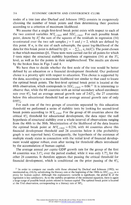
We assume that a single first-level break point exists with respect to each of the two control variables Myi1960 and SECi 1960* For each possible break point, denote by 6]j the sum of the squares of the residuals in regression (14) re-estimated over the two sub samples j = I and j = 2, which are defined by this point. If nj is the size of each subsample, the quasi log-likelihood of the data for this break point is defined by QL = - Z= 1 nj ln(Qj4). The point chosen is that which maximises QL. These tests were carried out for all points for which F-tests reject the structural stability hypothesis of regression (14) at the 5% level, as well as for the points in their neighbourhood. The results are shown by the broken lines in Figs 3 and 4.

We have then to decide whether the first node of the tree would be better defined by an education or a financial development threshold. Our preferred choice is a priority split with respect to education. This choice is supported by the data, according to a maximum likelihood test similar to that used to locate the optimal break points. The first-level optimal break point is located at the 69th observation, which corresponds to SECi 1960 = 0.06.21 It is interesting to observe that, while the 68 countries with an initial secondary school enrolment rate over 6% had an average annual growth rate of 2.62%, the 27 countries below this educational threshold had an average annual growth rate of only 0.95%.

For each one of the two groups of countries separated by this education threshold we performed a series of stability tests by looking for second-level break points according to M i 1960* For the group of 68 countries above the critical 6% threshold for educational development, the data reject the null hypothesis of structural stability over a whole interval of observations ranging from the 40th to the 50th. Maximization of the likelihood of the data locates the optimal break point at MY 1960 = 0.216, with 44 countries above this financial development threshold and 24 countries below it (the probability graph is not reported here). Consequently, the hypothesis of the existence of multiple steady states in connection with the initial level of financial development would appear robust, even after testing for threshold effects introduced by the accumulation of human capital.

The average annual per capita GDP growth rate for the group of the first 44 countries was 3.1% over the period studied, while it was only 1.7% for the other 24 countries. It therefore appears that passing the critical threshold for financial development, which is conditional on the prior passing of the 6%

21 In order to compare our results with those obtained by Durlauf and Johnson (1992), we reestimated eq. (14) by substituting the literacy rate at the beginning of the 1960s to SECj, 1960 as a proxy for human capital. Although this explanatory variable is significant, the global fit of the regression is less satisfactory. As to the stability properties of the estimated equation, there is again a large range of possible break-points related to human capital. The optimal break point is located at the 53rd observation, corresponding to a literacy rate of 50%o.




critical threshold for educational development, adds on average 1.4 percentage points to per capita GDP growth rate. This amounts to a 41% cumulative gain in per capita output over the life-span of a generation. A threshold associated with the initial level of financial development would also appear to exist for the 27 countries with low growth potential, due to a low initial level of education. We carried out the same stability analysis on regression (14) for this group of countries and identified a significant break point for M Y 1960 = 0.153, with 12 countries above this threshold and 15 countries below it. This threshold is virtually identical to the one we discovered for the main group of 68 countries. Our regression tree is therefore as follows:

> 6/ : 68 countries K M}1960 > 21.6% 44 countries (A)

\M} 1960 < 21.6% 24 countries (B) SECi. 1960

\ < 6%: 27 countries __M Yi, 15.3% 12 countries (C) \ \M 1960 < 15.3% 15 countries (D)

4.3. Stability tests on financial development and break points identification

As a further step to checking the existence of threshold effects with respect to initial financial development we investigate cross-country evidence on the determinants of the level of financial development at the end of the estimation period. If our theoretical conclusion about multiple equilibria is right and if the break points with respect to initial financial development are correctly identified, countries starting with M } 1960 below the relevant financial development threshold should be unable to significantly expand their financial sector, which could even contract. On the contrary, countries starting above this threshold should be expected to end up with a considerably more developed financial sector. Put differently, the break points we previously identified with respect to MYi 1960 should also be relevant in explaining the behaviour of our financial development indicator at the end of the estimation period, i.e., the behaviour of M Y 1985-

Our regression equation explains cross-country differences in the rate of growth of MY over the estimation period 1960-85, defined by DM Y = log(M Y 1985) - log(M 1i, 1960). Four explanatory variables are involved. Match- ing the specification of the growth regression, we use as a first explanatory variable the initial level of financial development measured by LM}, 1960 =

log(M Y 1960). This variable captures the idea of conditional convergence in the level of financial development: Countries starting with a smaller (bigger) financial sector can be expected to expand financial activities faster (slower) towards equilibrium after controlling for the proximate factors determining the equilibrium level of financial intermediation. Discovering global convergence in financial development, coupled with structural stability of the estimated equation, would amount to rejecting the assumption of multiple equilibria with respect to the initial level of financial development.

The average rate of inflation in consumer prices over the 1960-85 period




(DPi) is also included in the set of explanatory variables. Higher inflation increases the opportunity cost of holding money, leads to a comparatively lower MY ratio, and therefore inhibits financial development. Financial repression, in the form of interest rate controls, has been often used by governments as a means to lower the cost of loanable funds to investors or to the government itself. Severe financial repression, leading to persistently negative real interest rates, reduces financial savings and impedes financial development. This influence is captured by using as an explanatory variable the average level of the short-term real interest rate over the 1960-85 period. In order to construct a relatively homogeneous variable we use the Central Bank's discount rate as the relevant nominal interest rate, since this is the more broadly available interest rate over our 95 country data set. The real interest rate (RRi) is computed by subtracting observed consumer price inflation from the discount rate. It should be noted first that, due to lack of data on interest rates for a long enough time period, our sample for this estimation has been reduced to 85 countries.22 Secondly, for a few countries23 we use the deposit rate as the relevant short-term interest rate because of lack of data on the discount rate. This may however bias the estimated effect of financial repression in so far as the deposit rate is systematically lower than the discount rate. To take into account this imperfection of our data we use an appropriately defined dummy variable (DEPRi). Finally, we use LSECz 1960 as an additional explanatory variable, on the presumption that starting with a higher level of human capital raises both the efficiency of financial intermediaries and consumer demand for their services, leading therefore to a higher equilibrium level of financial intermediation.

The estimated equation with OLS (White estimator) is as follows

DMY=- 0.029 - 0.724LM1i,1960 + 0.158LSECi,1960 - 0.019DP,

(0.29) (6.61) (3.21) (3.69)

+ 0.014RRi + 0.369DEPR (15) (1.67) (2.16)

R= 0525 S.E.R. = 0.38 n. obs. 85

Skewness: 0.157 Kurtosis: 2.527 Jarque-Bera normality test: 1.141

As it can be observed, all estimated coefficients have the expected sign and are highly significant with the exception of the real interest rate which is significant at a 10% level. The negative coefficient of LMt 11960 indicates that countries starting with a smaller (bigger) financial sector tend to experience faster (slower) financial development. The positive coefficient of the real interest rate and the negative one of the inflation rate confirm the detrimental influence

22 The countries that have been dropped out of the sample are Algeria, Dominican Republic, El Salvador, Haiti, Iraq, Israel, Nicaragua, Panama, Paraguay, and Saudi Arabia.

23 Argentina, Chile, Indonesia, Mexico, Myanmar, Singapore, and Sudan. Data for consumer prices, interest rates, broad money supply and nominal GDP in 1985 are taken from IFS, IMF.




of financial repression and of inflationary policies on the development of the financial sector.24 The positive coefficient of LSEC1 1960 is of particular interest for long-run growth analysis. It means that educational development exerts both a direct effect on growth (shown by the corresponding coefficient in eq. (14)) and an indirect influence by enhancing financial development, which later feeds back on growth (see the MYi 1960 effect in eq. (14)). This joint influence of SEC, 1960 is consistent with our finding of the threshold on human capital having the priority over the financial development threshold.

In order to check the structural stability of eq. (15) with respect to the initial size of the financial sector we first sorted the 85 country sample in decreasing order by MYi 1960. Then we carried out successive one-break-point stability tests. The results clearly reveal a large range of possible break points of the estimated equation. Using the same maximum likelihood criterion as previously, we can locate the optimal break point at the 58th observation. The corresponding initial size of the financial sector as measured by our M Y 1960 indicator is 0. 189. As it can be observed, this threshold lies exactly between our two estimates of the threshold effect of financial development on growth, i.e. 0.153 and 0.216, depending on the initial level of educational development.

Consequently, the data clearly reveal the existence of a threshold effect related to the initial size of the financial sector, which is relevant to both subsequent financial development and long-run growth. Countries located below the estimated threshold experienced both slow growth and weak financial development, while countries located above it have grown faster and ended up with a much stronger financial sector. To get some more insights on financial development in the two groups of countries separated by the M i, 1960 = 0.189 threshold, we run two separate regressions shown in Table 1. As it can be observed, both groups of countries exhibit local convergence, shown by the significantly negative LM Yi, 1960 coefficient. Group-I countries, starting above the threshold, roughly reproduce the characteristics of regression (15). They moreover show a significantly detrimental influence of repressed real interest rates on financial development. In the case of countries located below the threshold, human capital does not exert any kind of influence on financial development. Inflation and financial repression policies seem to exert some- although not very strong influence on the equilibrium level of financial intermediation. The most important remaining factor is conditional convergence towards this low growth equilibrium.

The main observed differences between Group-I and Group-IL countries with respect to growth and financial development are summarized in Table 2. As it would be expected, average growth of real per capita GDP in group-I countries has been twice as high as in Group-IL countries. Furthermore, as shown by the M Y indicator, Group-I countries ended up with a considerably more developed financial sector in the mid 1980s than Group-LI countries. It should be noted

24 The positive coefficient of DEPRi is due to the fact that the deposit rate is lower than the discount rate. This biases downwards the contribution of the real interest rate to DM 1.




TABLE 1 Financial development regressions

(dependent variable. DM Y = LM Y1985 -LM Y1960)

Independent Equation 1 Equation 2 Variables Group I* Group IIt

Constant 0.145 -1.077 (1.07) (4.82)

LMY1960 -0.651 -0.872 (4.14) (8.72)

LSEC1960 0.154 0.001 (2.36) (0.01)

DP -0.025 -0.010 (3.84) (1.61)

RR 0.029 0.010 (2.99) (1.25)

DEPR -0.059 0.459 (0.70) (2.26)

Adjusted R2 0.419 0.717 SER 0.366 0.324 Skewness 0.078 0.383 Kurtosis 2.979 2.042 Jarque-Bera test 0.059 1.755

* MY1960 > 18.9>% (57 countries). t MY1960 > 18.9% (28 countries). In brackets: student's t-statistics.

TABLE 2 Comparative financial development of groups of

countries

Group I Group II

Growth, 1960-85 2.5% 1.4% M Y 960 0.37 0.13 M Y1985 0.55 0.29 MY* 0.59 0.28 M Y** 1.00 0.38

that the observed differences in Myi 1985 understate the underlying financial development capacity of the two groups. This is more adequately reflected in long-run equilibrium differences in MY ratios, computed on the basis of the regression results reported in Table 1. The MY* equilibrium levels shown in Table 2 are computed on the basis of the observed average levels of the explanatory variables (LSEC, DP, and RR) over the estimation period 1960-85 in the whole sample. They show slightly bigger differences in financial development than the observed MYs. The MY** equilibrium levels are computed on




the assumption that 'good economic policies' are implemented with respect to inflation and the financial sector. As a matter of fact, this calculation is based on zero inflation and a real short-term interest rate of 3%. This yields a long-run equilibrium level of MY in Group-I countries which is 2.6 times higher than the corresponding level in Group-IL countries.

5. Growth behaviour of convergence clubs

5.1. Countries with high initial educational development

The analysis of the estimated parameters for the global convergence equation previously tested shows that the first two groups (A and B) behave quite differently with respect to factors affecting long-run growth. Table 3 shows our best estimates of the conditional convergence equation for the two groups. In both cases, initial per capita income exerts a significant negative influence on subsequent growth, indicating conditional convergence within the group. This

TABLE 3 Grovwth regressions for the countries wit/i high initial

educational development (A and B) (dependent variable: L Y15,v -L Y/960)

Independent Equation 1 Equation 2 variables Group A* Group Bt

Constant 0.411 1.346 (5.86) (2.35)

LY1960 -0.379 -0.667 (4.73) (3.26)

LSEC1960 0.343 0.216 (4.08) (1.19)

GOV -1.989 3.135 (2.71) (2.71)

OPEN 0.283 -1.386 (4.44) (5.16)

MYl 960 0.462 (2.62)

REVC -0.484 (4.13)

OIL 0.309 (2.60)

Adjusted R2 0.526 0.578 SER 0.235 0.258 Skewness -0.231 0.458 Kurtosis 2.824 2.936 Jarque-Bera test 0.447 0.841

* SEC1960 , 6</, and MY1960 ) 21.6% (44 countries). t SEC,960 > 6" and M Y1960 < 21.6k, (24 countries). In brackets: student's t-statistics.




should be interpreted as additional evidence that the two groups of countries, which are separated by the financial development threshold, form distinct convergence clubs to different steady-state growth paths. In spite of their reasonably good initial educational situation, group-B countries would have been restricted to a relatively low standard of living due to the absence of sufficient financial services.

Group-A countries reproduce the broad characteristics of the global convergence equation (14) as regards the influence of public consumption, openness, education, and financial development. However, coups d'etat and the oil- production factor do not seem to play a significant role in this group of countries. The countries with high initial educational development, but with a low level of financial development (Group B), appear to behave differently. The financial development variable, to begin with, has no effect on growth: if the economy is financially repressed it seems to matter little whether this restraint is strong or weak. Next, the educational development indicator no more exerts a significant influence on growth. Such evidence suggests that lack of adequate financial intermediation services leads to a levelling-off of the effects of education on growth. This could be true if, for example, beyond a certain level of educational development, the benefits from the accumulation of human capital become conditional on changes in the sectoral allocation of investment, which are difficult to implement without a sufficiently developed system of financial intermediation.

Furthermore, it is interesting to observe that, while openness exerts a positive effect on growth in the case of financially developed countries, its influence turns out to be significantly negative in the case of Group-B countries. To explain such a finding we should bear in mind that for a country to reap the benefits from specialisation following a liberalization of foreign trade, it must be able to undertake significant intersectoral movements of factors of production according to comparative advantage. Such sectoral reallocations of labour and capital require, in turn, a well-functioning system of financial intermediation. With an insufficiently developed financial system these structural changes are presumably realized over a lengthy period of time, during which the economy suffers from job destruction and output losses, experiencing therefore a comparatively lower rate of growth. Moreover, a slow adaptation is costly in a context of rapid ongoing changes in the international market conditions.

Finally, we obtain also opposite effects on growth in these two groups of countries with respect to government consumption. While its impact is negative in the financially developed countries, this influence turns out to be significantly positive in the group of countries which lack an adequate financial structure. This paradox could perhaps be explained by the fact that government spending exerts, in principle, two opposing influences on growth: (i) a positive influence through the provision of public goods that may generate some kind of productivity-enhancing externalities; and, (ii) a negative influence in so far as government spending crowds out private savings in the presence of over- lapping- economically disconnected generations. It is then possible that the




crowding-out effect is dominated by the productivity-enhancing effect in the case of the Group-B countries, where the underdevelopment of the financial sector constitutes the main factor that inhibits the growth of private sector savings and investment. Moreover, in these countries, externalities generated by public goods are presumably the only potential source of endogenous growth due to the lack of private investment dynamism.

5.2. Countries with low initial educational development

Table 4 shows out best estimates of the conditional convergence equation (14) for the Groups C and D of countries located below the educational development threshold. Obviously, the small size of these two groups suggests some caution in interpreting the results. In this case too, the two groups of countries appear to behave quite differently. Our estimates suggest similar differences in patterns

TABLE 4 Growth regressions for the countries with low initial educational development

(C and D) (dependent variable: L Y1985 -L YJ96()

Independent Equation I Equation 2 Equation 3 variables Group C* Group Dt Groups C & D

Constant -0.498 -0.214 -0.314 (1.47) (1.93) (1.79)

LY1960 -0.488 -0.518 -0.487 (5.05) (5.51) (4.52)

GOV -5.347 (4.43)

GOV x DC -4.437 (3.81)

OPEN 1.002 (4.79)

OPEN x DC 1.206 (3.73)

MY1960 5.047 2.277 (5.17) (1.96)

REVC -1.591 -0.453 -0.849 (5.62) (2.87) (4.12)

OIL 0.670 0.556 0.554 (7.77) (1.90) (4.14)

Adjusted R2 0.934 0.633 0.747 SER 0.144 0.193 0.220 Skewness -0.007 -0.150 0.081 Kurtosis 1.823 2.879 2.604 Jarque-Bera test 0.692 0.065 0.206

* SEC1960 < 6%" and MY1960 ? 15.3%. (12 countries). t SEC1960 < 6%" and M Y1 960 < 15.30% (15 countries). DC = I for group-C countries, 0 otherwise. In brackets: student's t-statistics.




of growth with those observed in the case of the two groups, A and B, of countries located above the educational threshold. Growth in Group-C countries seems to be influenced by a set of factors quite similar to the one found in the case of financially developed Group-A countries. Government consumption exerts, in this case too, a detrimental influence on growth, openness exerts a positive effect, and a higher volume of financial services improves growth prospects. The main difference with Group-A countries is that the effect of educational development on growth now vanishes. This is quite natural, given that these countries are precisely located below the educational development threshold. As in the case of the threshold with respect to financial development, the beneficial effects of education on growth cannot materialize unless the critical level of human capital accumulation is reached.

The estimates for the last group of countries (D), which combine educational and financial development initial handicaps, reveals a complete absence of growth dynamics. The effect of the educational development, financial development, government expenditure and openness variables on these 15 countries is totally non-existent. The only remaining explanatory factors are the effect of fl-convergence, the effect of revolutions and coups d'&tat and the possession of oil resources. To partially overcome the reliability problem of these estimates due to the small size of the two samples, we estimated a common regression for Groups C and D with appropriately defined dummy variables for government spending and openness. The results (eq. (3)) confirm the direction of effects obtained over the separate samples, and lead, quite naturally, to a reduction in the magnitude of the estimated parameters.

We finally used the same method of estimation -consisting in differentiating the effects by groups of countries through use of dummy variables in order to globally check the individual group results over the whole sample of 95

2 5 countries. Our estimates appear in table Al of the appendix. As it can be observed: (i) all groups exhibit significant internal /1-convergence; (ii) education has a significant influence on growth only in countries already above the educational and financial development thresholds; (iii) government spending has a detrimental influence on growth in financially developed countries (irrespective of education), but a positive one, in financially repressed countries; (iv) the volume of financial services produced only matters after the relevant threshold of financial development has been passed; and (v) openness does increase growth in financially developed countries (again irrespective of education), but seems to be harmful in the absence of an adequate structure of financial intermediation for countries with a high level of education. For Group D openness has now a positive effect, but much smaller than for Group C.

25 We thank Maxwell Fry for suggesting to us this method for checking the results. Estimating each group's growth coefficients over the whole sample-using dummy variables to distinguish the groups-implicitly constrains the variance of the error term to be the same for the four groups. On the contrary, estimating four growth regressions separately allows this variance to vary. The results presented in Tables 1 and 2 and in the Appendix check for these differences in error variances.




TABLE 5 Comparative peiformances of groups of countries

Growth Hypothetical 1960-85 IN V/GDP GDPJ985 stationary M Y1960) SECJ960) OPEN

Group (2o) (JO) '000 $/cap GDP/cap (A (0jX (A

A 3.1 22.8 6.1 17.2 43.1 37.3 65.8

B 1.7 18.6 2.5 2.7 15.9 19.3 49.4

C 1.3 13.8 1.4 1.3 20.9 3.2 63.8

D 0.7 12.6 0.5 0.5 10.7 2.4 43.3

>> (>) significantly higher at the 1% (5%) level. << Significantly lower at the 1% level.

5.3. Comparative performance of convergence clubs

In order to check whether the previously identified groups form distinctive convergence clubs, it is useful to examine the properties of their respective long-run growth paths. A first analytical approach consists of simply comparing the average performances of these groups over the estimation period from 1960 to 1985. Some useful indicators for this are given in Table 5: the average annual growth rate, the average investment ratio, and the level of per capita income reached in 1985. We also included information on the initial levels of educational development, financial development, and average openness degree of the economy, to be able to more precisely characterise the different groups. The composition of each group is shown in Table A2 in the appendix.

The clearest split with respect to growth rates appears between Groups A and B, comprising countries with sufficient human capital, which are located on either side of the financial development threshold. The same phenomenon can be observed when comparing the investment rates. Moreover, the intuition according to which the investment ratio is endogenously linked to financial development is borne out when the first two groups are compared: A-countries have a significantly higher investment ratio than B-countries. Nonetheless, there is also a substantial difference in investment ratios between the countries with high (A, B) and the countries with low (C, D) initial educational development. This would seem to suggest that investment could also be influenced by the availability of human capital.

The observed difference in investment ratios between Group-A and Group-B countries is sufficient, on an accounting basis, to explain their difference in growth performance. Using a rough estimate of 3 for the capital/output ratio, the 4.2 percentage points increase in the investment ratio associated with the significantly higher level of financial development exactly accounts for the 1.4 percentage points increase in the annual growth rate of per capita output. Conversely, the 0.4 percentage points difference in growth rates between Groups




B and C is too small to be accounted for by the 4.8 percentage points rise in the investment ratio, associated with an adequate level of educational development. This could be interpreted as evidence of a lower productivity of investment, due to the lack of a sufficiently developed system of financial intermediation (since B-countries are, precisely, located below the financial development threshold).

This evidence suggests that the Group A is clearly a convergence club, made up of the countries that were, on the whole, on a high growth path over the 1960-1985 period and had high per capita income at the end of the period. The Group B presumably forms a second convergence club, corresponding to a relative poverty trap, incorporating countries with sufficient initial human capital to take off, but a financial system lacking in efficiency. This B group contains the vast majority of our sample's Latin American countries, which have a long-standing tradition in implementing financial repression policies. Nevertheless, one country in this group, Korea, is an exception. Korea is renowned for its successful takeoff based on a set of suitable policies over the period from 1960 to 1985. One of these policies was moderate financial repression, which enabled capital to be allocated in a relatively efficient way and thereby accelerated its development (see Stiglitz 1993). Conversely our Group A actually contains a number of countries (essentially in the Middle-East zone) which, although starting with favourable conditions with regard to financial development and education, failed to catch up with advanced OECD countries because of inadequate policies during this period and, presumably, also because of wars.

Group D apparently forms a convergence club around a poverty trap, comprising the countries that initially combine handicaps in the form of both low financial development and absence of human capital. It should be remembered that our econometric results for these countries contain only non-economic variables such as coups d'etat or the availability of oil resources to explain growth, which definitely suggests the absence of growth dynamics. Group C is more difficult to characterise, since it contains countries whose take-off could be definitely impeded in so far as the educational development threshold has some priority over financial development. These countries could therefore be in a state of transition, either regressing towards the poverty trap formed by the D-group countries, or drawn upwards by the B-group (and, then possibly by the A-group) countries. To that end, good policies would certainly be of substantial aid, since growth dynamics in C-group countries are significantly influenced by finance, openness, and government spending (see Table 4).

If we assume that all the exogenous variables including the exogenous technological progress picked up in the regression intercept are likely to remain unchanged in the long run at their average value for each group, we can then calculate a hypothetical level of long-run per capita income by inverting the conditional /-convergence equation. This calculation might not replicate future growth paths, but it does illustrate the underlying differences




in long-run trends of our three most likely convergence clubs. We therefore find (fifth column of Table 5) a long-run per capita GDP of approximately $17,200 for the convergence club of financially and educationally developed countries (group A); $2,700 for the intermediate convergence club (B); and $500 for the countries in a poverty trap (D). Although these differences are hypothetical, they give a good illustration of the impact that suitable education and financial- sector policies can have in the long run.

6. Conclusion

The introduction of reciprocal interactions between the financial sector and the real sector into a growth model naturally reveals the possibility for multiple steady state equilibria of endogenous growth: the conjunction of the financial sector's positive influence on capital efficiency and the real sector's external effect on the financial sector via the volume of savings generates a cumulative process, which is a potential source of poverty traps.

To test this theoretical framework, considerations beyond the relations between financial development and growth need to be introduced. A number of other potential poverty traps have actually been identified in growth theory, especially with respect to the accumulation of human capital. Neglecting these alternative sources of poverty traps could lead to an erroneous diagnosis of the reasons for an economy's stagnation or taking off, and consequently to biased estimates of growth equations due to the existence of a significant correlation between the various possible origins of poverty traps.

Therefore, to make this kind of theory operational, it is essential to build convergence club tests that accept several possible origins for poverty traps. This is precisely what we have attempted here, by identifying jointly, through a maximum likelihood method, break points associated with both educational development and financial development. Our results show that the former is a pre-condition for growth, while financial underdevelopment may become a particularly severe obstacle to growth in countries where that pre-condition is satisfied. This seems for instance to be true for a large number of Latin American countries, well known for their financial repression policies in the 1960s and I 970s. It is also shown that the optimal policies in other areas, i.e. in our analysis trade policy and government expenditure policy, depend on the absence or presence of a reasonably well-developed financial system. For countries which belong to the financially underdeveloped categories, economic openness does not seem to exert a positive impact on growth, while government expenditure has a positive effect. These results show that the second best policies in countries which have not succeeded in developing a financial system might be quite different from the policies usually advocated in a first best framework. It should be therefore advisable to establish as early as possible policies which would avoid a heavy repression of the financial system, in order to be able to pursue optimal policies in other areas.




ACKNOWLEDGEMENTS

Helpful comments by A. Courakis, M. Fry, J. De Gregorio, and two anonymous referees are gratefully acknowledged. Responsibility for any errors and omissions remains of course with the authors.

REFERENCES

ATJE, R. and JOVANOVIC, B. (1994). 'Finance and Development', unpublished paper, New York University, February.

AZARIADIS, C. and DRAZEN, A. (1990). 'Threshold Externalities in Economic Development', Quarterly Journal of Economics, 105, 501-26.

BARRO, R. J. (1991). 'Economic Growth in a Cross Section of Countries', Quarterly Journal of Economics, 106, 407-43.

BARRO, R. J. and SALA-I-MARTIN, X. (1992). 'Convergence'. Journal of Political Economy, 100, 223-51.

BECKER, G. S., MURPHY, K. M., and TAMURA, R. (1990). 'Human Capital, Fertility, and Economic Growth', Journal of Political Economy, 98, 12-37.

BENCIVENGA, V. R. and SMITH, B. D. (1991). 'Financial Intermediation and Endogenous Growth', Review of Economic Studies, 58, 195-209.

CHATTERJI, M. (1993). 'Convergence Clubs and Endogeneous Growth', Oxford Review of Economic Policy, 8, 57-69.

DE GREGORIO, J. (1993). 'Credit Markets and Stagnation in an Endogenous Growth Model', Working Paper 93/72, International Monetary Fund, Washington, DC.

DOLLAR, D. (1992). 'Outward-oriented Developing Economies Really Do Grow More Rapidly: Evidence from 95 LDCs, 1976-1985', Economic Development and Cultural Change, 40, 523-44.

DURLAUF, S. N. and JOHNSON, P. A. (1992). 'Local versus Global Convergence Across National Economies', Discussion Paper No. 131, LSE Financial Market Group, London.

EDWARDS, S. (1993). 'Openness, Trade Liberalization, and Growth in Developing Countries', Journal of Economic Literature, 31, 1358-93.

FRY, M. J. (1988). Money, Interest, and Banking in Economic Development, The Johns Hopkins University Press, Baltimore.

GREENWOOD, J. and JOVANOVIC, B. (1990). 'Financial Development, Growth, and the Distribution of Income', Journal of Political Economy, 98, 1076-107.

GROSSMAN, G. M. and HELPMAN, E. (1991). Innovation and Growth in the Global Economy, MIT Press, Cambridge, MA.

KING, R. G. and LEVINE, R. (1993a). 'Finance, Entrepreneurship and Growth: Theory and Evidence', Journal of Monetary Economics, 32, 513-42.

King, R. G. and LEVINE, R. (1993b). 'Finance and Growth: Schumpeter Might Be Right', Quarterly Journal of Economics, 108, 717-37.

LEE, J.-W. (1993). 'International Trade, Distortions, and Long-Run Economic Growth', IMF Staff Papers, 40, 299-328.

LEVINE, R. (1991). 'Stock Markets, Growth, and Tax Policy', Journal of Finance, 46, 1445-65. LEVINE, R. and ZERVOS, S. (1993). 'Looking at the Facts: What we Know about Policy and Growth

from Cross-Country Analysis', American Economic Review, 83, 426-30. MANKIW, G. N., ROMER, D., and WEIL, D. N. (1992). 'A Contribution to the Empirics of Economic

Growth', Quarterly Journal of Economics, 107, 407-37. NEHRU, V., SWANSON, E., and DUBEY, A. (1995). 'A New Database on Human Capital Stock in

Developing and Industrial Countries: Sources, Methodology, and Results', Journal of Develop- ment Economics, 46, 379-402.

PAGANO, M. (1993). 'Financial Markets and Growth: An Overview', European Economic Review, 37, 613-22.

REBELO, S. (1991). 'Long-Run Policy Analysis and Long-Run Growth', Journal of Political Economy, 99, 500-21.




REBELO, S. (1992). 'Growth in Open Economies', Discussion Paper No. 667, Centre for Economic Policy Research, London (August).

ROMER, P. M. (1986). 'Increasing Returns and Long-Run Growth', Journal of Political Economy, 94, 1002-37.

RoUBINI, N. and SALA-I-MARTIN, X. (1992). 'A Growth Model of Inflation, Tax Evasion, and Financial Repression', Working Paper No. 4062, National Bureau of Economic Research, Cambridge, MA.

SACHS, J. D. and WARNER, J. (1995). 'Economic Reform and the Process of Global Integration', Brookings Papers on Economic Activity, 1, 1-118.

SAINT-PAUL, G. (1992). 'Technological Choice, Financial Markets and Economic Development', European Economic Review, 36, 763-81.

STIGLITZ, J. E. (1993). 'The Role of the State in Financial Markets', World Bank Annual Conference on Development Economics, Washington, DC.

SUSSMAN, 0. (1993). 'A Theory of Financial Development', in A. Giovannini (ed.), Finance and Development: Issues and Experience, Cambridge University Press, Cambridge, 29-57.

APPENDIX

TABLE Al Regression estimated onl the whole sample by differentiating the effects of independent variables

according to groups of countries (dependent variable: LY1985 - LY1960)

Variable\country group Group A Group B Group C Group D Regression 14

LY1 960 - 0.377 -0.699 -0.475 -0.679 -0.321 (3.53) (3.98) (5.04) (5.27)

MY1960 0.523 - 2.328 4.926 - 4.541 0.602 (2.61) (2.05) (4.47) (2.23)

LSEC1960 0.389 0.208 0.037 0.232 0.256 (3.48) (1.40) (0.24) (2.34)

GOV - 1.91 3.004 - 5.185 2.764 - 1.288 (2.37) (4.11) (4.52) (1.77)

OPEN 0.312 - 1.288 0.974 0.421 0.269 (4.22) (5.07) (3.86) (2.99)

REV 0.346 -0.653 - 1.585 -0.047 -0.312 (1.75) (4.02) (7.33) (0.38)

OIL 0.058 0.366 0.676 0.71 0.244 (0.44) (3.24) (9.12) (2.65)

Adjusted R2: 0.744; SER: 0.227; No. obs. 95. Skewness: 0.1 13; Kurtosis: 3.404; Jarque-Bera normality test: 0.848. Group-A: (SEC,1960 6%V and MY1960 1 21.6%V). Group-B: (SEC,196(0 6% and MY1960 ) 21.60?). Group-C: (SEC196(0 < 6%"( and MY196(0 > 15.3,). Group-D: (SEC1960 < 6%V and MY1960 < 15.3%/).




TABLE A2 Composition of the groups of countries

Group A Group B Group C Group D

Algeria Argentina Cameroon Benin Australia Bolivia Congo Burundi Austria Brazil C6te dIvoire Ethiopia Barbados Chile Gabon Haiti Belgium Colombia Gambia Indonesia Canada Costa Rica Ghana Malawi Cyprus Dominican Rep. Kenya Mauritania Denmark Ecuador Madagascar Nepal Egypt El Salvador Morocco Niger Fiji Guatemala Saudi Arabia Nigeria Finland Guyana Senegal Rwanda France Honduras Zafre Sierra Leone Germany Iran Sudan Greece Israel Togo Iceland Jamaica Zambia India Korea Iraq Mexico Ireland Nicaragua Italy Panama Japan Paraguay Jordan Peru Malaysia Philippines Malta Turkey Mauritius Venezuela Myanmar Netherlands New Zealand Norway Pakistan Portugal Singapore South Africa Spain Sri Lanka Sweden Switzerland Syria Taiwan Thailand Trinidad Tunisia United Kingdom United States Uruguay



Documents

Economic Growth, Convergence Clubs, and the Role of Financial Development