ECONOMIC GROWTH AND THE EXTERNAL SECTOR: EVIDENCE …

ECONOMIC GROWTH AND THE EXTERNAL SECTOR:EVIDENCE FROM KOREA, LESSONS FOR MEXICO∗

Julen Berasaluce

Jose Romero

El Colegio de Mexico

Resumen: Se realiza un analisis empırico del sector externo coreano entre 1980

y 2015 a fin de identificar las potenciales relaciones entre crecimiento

economico, exportaciones, importaciones e inversion extranjera directa.

Se eligio Corea porque ha sido considerado como una referencia de la

hipotesis de crecimiento a partir de las exportaciones, lo que ha justifi-

cado polıticas de promocion de las mismas en Mexico. Los resultados

de nuestro modelo de vectores autorregresivos de cuatro variables su-

gieren que las exportaciones y la inversion extranjera directa no son

las causantes del crecimiento economico coreano. Por lo tanto, de-

berıamos ser cautelosos antes de emprender polıticas que promuevan

estas magnitudes como herramientas de potenciacion del crecimiento

economico.

Abstract: In this paper, we have set up an empirical analysis of the Korean

external sector between 1980 and 2015, in order to identify the potential

relationships between economic growth, exports, imports and foreign

direct investment. We chose to study Korea because is a country that

has been taken as a reference of the export-led growth hypothesis in

order to justify export-promoting policies in Mexico. The results of

our four-variable vector autoregressive model suggest that exports and

foreign direct investment are not driving economic growth in Korea.

Therefore, one should be cautious about policies that promote such

investment and export tools to boost economic growth.

Clasificacion JEL/JEL Classification: C31, F14, F43

Palabras clave/keywords: South Korea, VAR, industrial policy, exports, imports,

FDI, growth, Corea del Sur, polıtica industrial, exportaciones, importaciones,

crecimiento

Fecha de recepcion: 02 II 2016 Fecha de aceptacion: 11 VII 2016

∗ [email protected], [email protected].

Estudios Economicos, vol. 32 num. 1, enero-junio 2017, paginas 95-131

96 ESTUDIOS ECONOMICOS

1. Introduction

The Republic of Korea, generally identified as one of the Asian tigers,has received much attention due to its phenomenal growth in re-cent decades. For some, this is the result of market-friendly policies(see Westphal, 1978, Krueger, 1979 and World Bank, 1993); for oth-ers, it derived from the actions taken by “the developmental state”(see Amsden, 1989, Haggard, 1990 and Woo-Cumings, 1999). Itsgrowth strategy has sometimes been oversimplified and described asan export-led growth model, as if Korea’s success could be solely ex-plained by its export promotion. While the Korean government didindeed actively promote exports during the 1960s and 1970s, its de-velopment policy was much more complex and far-reaching (Chang,1994).

The variety of policies implemented and the particularities of theKorean economy generated a particular causal relationship betweeneconomic growth and the external sector. This process was the resultof a successful strategy that consisted in fostering the creation anddevelopment of competitive firms, so they could achieve world-classstatus. Once they reached such a level, Korean firms did not need asmuch protection as those of other countries; exports came as a naturalresult of their level of efficiency. Korea’s success should not be seenas the expected outcome of a liberalization process, but rather as theresult of a specific development strategy applied step by step underthese specific circumstances. In order to give a better explanation ofthe causality effects found in the quantitative analysis, we begin witha brief historical review of the development and industrial policiescarried out by the Korean government, focusing on those that arerelated to the external sector, as well as of some key points of itsliberalization process.

The Korean economy has shown consistent real GDP per capitagrowth (5.24% average annual real growth from 1950 to 2015). Theeconomic policies carried out by Korea have transformed the coun-try from a rural economy into an industrialized one, through themost rapid developing process that any country has ever experienced.Given its results, the Korean case must constitute an example of poli-cies to be considered by a developing country (see figure 1).

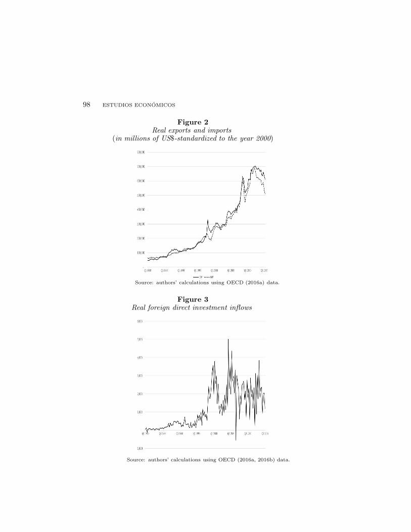
Misleadingly, Korea has been described as an example of theexport-led growth model. As we can observe in figure 2, Korea’sinternational trade, expressed in terms of real exports and imports,has grown enormously over the last decades. As a frame of reference,Korea’s real exports in the second quarter of 2014 were 13 times thoseof the first quarter in 1980, while imports grew 8 times during the

ECONOMIC GROWTH AND THE EXTERNAL SECTOR 97

same period. Indeed, although the fast economic growth in Koreawas accompanied by rapid growth in exports, we shall not rush intoconclusions about the direction of causality.

Following the Japanese example, one of the key characteristics ofthe Korean strategy was to limit the access of foreign direct invest-ment (FDI) to the Korean economy, although it was forced to partiallyliberalize after the Asian crisis in the nineties. Consequently, FDI ex-perienced a rapid growth after the 1997 crisis and changes in regula-tion, but stagnated after 2000, within a narrow range of variability(see figure 3).

The purpose of this study is to analyze the causal relationshipsbetween the Korean foreign sector and its economic growth and totest the traditional hypothesis of the sources of economic growth. Wedo that by estimating and analyzing a VAR (vector autoregresion)model with four variables (GDP, exports, imports and FDI), sincethe 1980s. The study tests the long-run and short-run relationshipsbetween GDP, exports, imports and FDI for Korea from 1980Q1 to2015Q1 using quarterly data. This paper contributes to the debateon the sources of Korea’s economic growth, as well as to the literatureon the connection between economic growth, trade liberalization andindustrial policies.

Figure 1Annual GDP per capita in 1990 US$

(converted at geary khamis PPPS)

Source: Conference Board (2015).


Figure 2Real exports and imports

(in millions of US$-standardized to the year 2000)

Source: authors’ calculations using OECD (2016a) data.

Figure 3Real foreign direct investment inflows

Source: authors’ calculations using OECD (2016a, 2016b) data.


Our methodology is close to that used by Nguyen (2011), whoimplements a set of econometric procedures, including the unit roottest of four series, lag structure, the VAR diagnostic, the Johansenco-integration test, the Granger Causality/Block Exogeneity WaldTest (GCBEW test), analysis of impulse response and analysis of vari-ance decomposition, to study the impact of trade liberalization onMalaysian and South Korean economic growth using annual data.This methodology is relevant for our study for two reasons. First,it has the advantage of avoiding misspecification and minimizing theresulting omitted-variables bias. Second, it allows us to test and esti-mate the causal relationship among variables (GDP, exports, importsand FDI) through a four-variable VAR model.

The remainder of the paper is organized as follows. The secondsection presents a brief literature review. The third describes thedata set. The fourth section explains the methodology as well as theestimation results. The conclusions are given in the fifth section.

2. Literature review

Korean industrialization took off under the rule of Park Chung-hee,who, through an intense industrial policy, created rents in order topromote selected sectors. Together with protectionist policies, thegovernment promoted exports both to finance the necessary importsand as a measure of the improvement in competitiveness of firms, inorder to justify the access of these firms to subsidies and a protectednational market.

After the death of Park Chung-hee and the short-lived govern-ment of Choi Kyu-hah, Chun Doo-hwan took power through a coupd’etat in 1980 and began a slow process of liberalization, which min-imized its potential negative impact. Korea still kept some of theinstitutions that were created following the logic of the developmen-tal state, such as the Korean Trade Promotion Corporation (KOTRA).Current president Park Geun-hye’s strategy of promoting the creativeeconomy shows that the Korean interventionist industrial policy didnot disappear with the arrival of democracy nor with the 1997 crisis.In any case, even though the rapid economic growth of the liberalizingperiod starting in 1980 must be seen as the consequence of the poli-cies adopted during Park Chung-hee’s regime, those periods shouldnot be analyzed together due to the high degree of intervention of hispolicies.

Trade liberalization may have a negative impact on developingcountries because of the increase of imports, which worsen the trade


balance (Santos-Paulino and Thirlwall, 2004). The magnitude of theimpact on exports or imports depends on the country and on its initialconditions, as shown by Awokuse (2007).

Since the 1970’s, there has been a considerable shift towards ex-port promotion strategies in most of the developing world, supportedby the idea that export expansion leads to better resource alloca-tion, “creating economies of scale and production efficiency throughtechnological development, capital formation, and employment gen-eration” (Shirazi and Abdul-Manap, 2005: 472). The success of theoutward-oriented policies of the East Asian Tigers provoked a greatdeal of consensus over the export-led growth hypothesis. It was notjust accepted by academicians (see Feder, 1983 and Krueger, 1980),but it evolved into a “new conventional wisdom” (Tyler, 1981, Bal-assa, 1985). Several countries followed these policy recommendations,which were also promoted by institutions the World Bank (1987).

However, the export-led growth hypothesis has been questionedin recent times. Ahmad and Harnhirun (1995) did not find a goodbasis to confirm the hypothesis of export-led growth for the ASEAN re-gion (Indonesia, Malaysia, the Philippines, Singapore and Thailand).Instead, they claimed that the interaction of exports with interiormechanisms could be a more suitable explanation for the economicgrowth of these countries.

Although imports could, at least theoretically, increase growthbecause of the access to a greater market of intermediate inputs andthe improvement of competitiveness, they can also destroy the do-mestic productive chains, reallocating the domestic resources fromproductive employment to unemployment.

The cautious observations of liberalization processes and the dy-namics between growth and the external sector in different countries,especially the Asian ones, are of great importance for Latin Americancountries. They are of particular interest for countries such as Mex-ico, Argentina, Brazil, Peru and Uruguay, where the twentieth cen-tury saw a significant increase in the elasticity of the ratio of exportsand imports with respect to income, (Guerrero de Lizardi, 2006).

FDI is, along with exports and imports, a key variable in explain-ing the relationship between a country and its external sector. Whenpurchasing goods abroad, companies can, basically, decide betweenimporting those goods or producing them in the foreign country, de-pending on the comparative advantages of either option. Companiesface a similar choice between investing in a foreign country and ex-porting their goods to such market. Because of these substitutabili-ties, FDI has also been studied, along with foreign trade, to determine


its relationship with economic growth. The choice between exportsand FDI depends on the level of convenience, risk, profit and long-rundeveloping strategy of firms, competitors, etc. (Liu, Wang and Wei,2001). Although FDI may increase capital and, therefore, production,it may also crowd-out domestic firms, so its total effect in developingcountries might be negative (see Herzer, 2012).

There are a significant number of studies on the relation betweeneconomic growth, export and FDI. Jung and Marshall (1985) performcausality tests between exports and growth for 37 developing coun-tries; the results cast considerable doubt on the validity of the exportpromotion hypothesis. Henriques and Sadorsky (1996) investigate theexport-led growth hypothesis for Canada by constructing a vector au-toregression (VAR) in order to test for Granger causality between realCanadian exports, real Canadian GDP, and Canada’s real terms oftrade; they find that these variables are co-integrated and evidence ofa one-way Granger causal relationship in Canada whereby changes inGDP precede changes in exports (i.e. growth-driven exports hypoth-esis). Zestos and Tao (2002) study the relations between the growthrates of exports, imports, and the GDP, for the 1948-1996 periodfor Canada and the United States, finding bidirectional causality forCanada from the foreign sector to GDP and vice versa, and a weakerrelationship between the foreign sector and GDP for the United States.

Konya (2004) investigates the possibility of export-led growthand growth-driven export by testing for Granger causality betweenthe logarithms of real exports and real GDP in twenty-five OECD coun-tries with annual data for the 1960-1997 period, and finds mixedresults.1 Shirazi and Abdul-Manap (2005) examine the export-ledgrowth hypothesis for five South Asian countries through cointegra-tion and multivariate Granger causality tests, and they also findmixed results.2 Liu, Shu and Sinclair (2009) look for causal rela-tionships between foreign trade, FDI and growth in a panel of Asian

1 “There is no causality between exports and growth (NC) in Luxembourg andin the Netherlands, exports cause growth (ECG) in Iceland, growth causes exports

(GCE) in Canada, Japan and Korea, and there is two-way causality between

exports and growth (TWC) in Sweden and in the UK.” (Konya, 2004: 73).2 “Feedback effects between exports and GDP for Bangladesh and Nepal and

unidirectional causality from exports to output in the case of Pakistan were found.

No causality between these variables was found for Sri Lanka and India, althoughfor India GDP and exports did induce imports. A feedback effect between imports

and GDP was also documented for Pakistan, Bangladesh, and Nepal, as well asunidirectional causality from imports to output growth for Sri Lanka.” (Shirazi y

Abdul-Manap, 2005: 472).


economies and reject any of the considered variables to be exogenous.Our paper is methodologically close to that of Nguyen (2011),

who analyzes the impact of trade liberalization on economic growthfor Malaysia and South Korea; he uses a four variable vector autore-gression (VAR) to study the relationship between trade, FDI and eco-nomic growth over the time period from 1970 to 2004 (for Malaysia)and from 1976 to 2007 (for Korea). Unlike Nguyen, we do not con-sider data from the 1970’s, since the Fourth Republic was a veryinterventionist period in Korea. The exclusion of those years is morethan compensated for by the use of quarterly data, which enrichesthe sample.

We coincide on denying any causal relationship from FDI on anyof the other variables and on the negative impact of imports on GDP.Unlike Nguyen, we find a positive causal relationship from GDP onboth exports and imports. Also contrary to Nguyen, we do not findcausal relationships from GDP on FDI, neither from exports on FDI

or GDP. According to the last one, we would reject the exports-ledgwroth hypothesis for Korea, which might have important implica-tions for countries such as Mexico. It might be the case that thedata from the highly intervened 1970s explained the absent causali-ties. FDI seems to consolidate in Korea as a substitute of imports. Itcould also be the case that the causalities found by Nguyen are drivenby a data set (1976-2007) that contains, relatively to its size, a higherproportion of institutional changes, such as changes in trade policy.

3. The data set

We use quarterly data from Q1-1980 to Q1-2015. The four time seriesare (see figure 4):

LRGDP (logarithm of real GDP)

LREXP (logarithm of real exports)

LRIMP (logarithm of real imports)

LRFDIL (logarithm of real FDI liabilities).

The data has been sourced from the OECD (2016a, 2016b) statis-tics. In order to express them in real terms, we have taken the seriesin current prices and transformed them by using a GDP deflator, sothat all variables were expressed in millions of 2000 US dollars beforetaking logs. Due to the high volatility of FDI, when analyzing quar-terly data, we have considered the average FDI of the last four periodsbefore taking logs.


Figure 4The four time series: LRGDP,

LREXP, LRIM and LRFDIL

4. Estimations

In this section, we estimate the relationships among the four variables.In order to do so, we follow Nguyen (2011) and perform the followingsteps:

1. Unit root test of four time series

2. Test the lag-length of the VAR model

3. Estimate four variable VAR model

4. VAR diagnostics (residual autocorrelation and residualnormality tests)

5. Johansen cointegration test


6. Granger causality Wald test

7. Dynamic simulation (impulse response function and variancedecomposition).

4.1. Estimation, tests and Granger causality

We begin by implementing a unit root test on our four series (LRGDP,LREXP, LRIMP and LRFDIL) by using the Phillip-Perron test. Ifall series are found to be I(1), they will be used in a four variable VAR.Table 1 and table 2 provide the evidence that the four time series arenon-stationary of order one.

Table 1Philips-Perron test (levels)

Variables Intercept Trend and intercept

LRGDP -5.4178 -1.1821

LREXP -1.1747 -2.7393

LRIMP -0.8241 -2.9459

LRFDIL -2.7817 -1.9240

Note: the critical values for the PP test with intercept

and with trend and intercept at the 1%, 5% and 10% signifi-

cance levels are respectively: -3.4785, -2.8826, -2.5781; -4.0264,

-3.4430, -3.1462.

The results from unit root tests in levels reported in table 1show that for most tests we cannot reject the null hypothesis (non-stationary) at a 0.01 significant level. LRGDP is clearly growingover time (see figure 4) so the appropriate test requires to inclusionof a trend and intercept (Elder and Kennedy, 2001). Thus, all thevariables have a unit root and we need to test the unit root of theirfirst difference.


Table 2Philips-Perron test(first differences)

Variables Trend and intercept

LRGDP -10.0479

LREXP -10.6823

LRIMP -9.8883

LRFDIL -12.9157

Note: the critical values for the PP test at

the 1%, 5% and 10% significance levels are:

-4.0269, -3.4432, -3.1463.

Since their absolute values are higher, in absolute values, thanthe 1 percent critical level, we can reject the null hypothesis of non-stationary. Thus, we can conclude that the four series in levels arenon-stationary with the root of order 1 (for robustness: see the resultsof the standard Augmented Dickey-Fuller (ADF) and Dickey-Fullertests for Generalized Least Squares (DFGLS) in Appendix). There-fore, we can proceed to construct a four-variable VAR model. Now,following Shin and Pesaran (1998), consider a four-variable (unstruc-tured form) standard VAR model of order p as:

yt =

p∑

(i=1)

Ai yt−i + Bxi + et (1)

where yt = (LRGDP, LREXP, LRIMP and LRFDIL) is a 4 × 1random vector; Ai is 4 × 4 fixed coefficient matrix; p is order of lags;xi is a d × 1 vector of exogenous variables; B is a 4 × d coefficientmatrix; and et 4 × 1 vector of error terms. As exogenous variables,we use nine dummy variables which ensure the normality of errors:

D1: 1981Q3=1, D2: 1986Q1=1, D3: 1988Q1=1, D4: 1988Q2=1,D5: 1989Q1; D6: 1998Q1=1, D7: 1998Q2=1, D8: 2008Q4=1, D9:2009Q1=1

The first five refer to political events: the effects of the instabil-ity of the creation of the Fifth Republic (1981Q3); the arrival of FDI

related to the Asian Games and preparation for the Olympic Games(1986Q1); the end of the Fifth Republic (1988Q1 and 1988Q2) andpolitical instabilities related to the demand for a greater democrati-zation (1989Q1). The last four are related to the 1997 Asian financial


crisis (1998Q1 and 1998Q2) and global financial crises (2008Q4 and2009Q1).

As claimed by Shin and Pesaran (1998) and Nguyen (2011), weare making the following assumptions:

• Assumption 1: E[εt] = 0, E[εtε′

t] =∑

, while E[εtε′

t′ ] = 0

when t = t′

and E[εt/wt] = 0.

• Assumption 2: All the roots lie outside the unit circle.

• Assumption 3: yt−1, yt−2...yt−p, xt... are not perfectly collinear

In addition to the selection of the lag order we will test for VAR

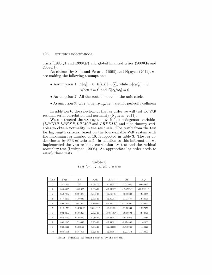
residual serial correlation and normality (Nguyen, 2011).We constructed the VAR system with four endogenous variables

(LRGDP, LREXP, LRIMP and LRFDIL) and nine dummy vari-ables to obtain normality in the residuals. The result from the testfor lag length criteria, based on the four-variable VAR system withthe maximum lag number of 10, is reported in table 3. The lag or-der chosen by FPE criteria is 5. In addition to this information, weimplemented the VAR residual correlation LM test and the residualnormality test (Lutkepohl, 2005). An appropriate lag order needs tosatisfy those tests.

Table 3Test for lag length criteria

Lag LogL LR FPE AIC SC HQ

0 12.51564 NA 1.03e-05 -0.133057 -0.043931 -0.096845

1 846.8335 1603.455 2.88e-11 -12.91927 -12.47364* -12.73821*

2 859.7092 23.94073 3.03e-11 -12.87046 -12.06832 -12.54455

3 877.4405 31.86087 2.95e-11 -12.89751 -11.73887 -12.42675

4 895.2069 30.81370 2.88e-11 -12.92511 -11.40997 -12.30950

5 918.1753 38.40032* 2.60e-11* -13.03399 -11.13234 -12.27353

6 934.2457 25.86325 2.62e-11 -13.03509* -10.80694 -12.12978

7 940.5769 9.793610 3.08e-11 -12.88401 -10.29936 -11.83386

8 952.2245 17.28943 3.35e-11 -12.81601 -9.874852 -11.62100

9 969.8641 25.08124 3.33e-11 -12.84163 -9.543966 -11.50177

10 988.6808 25.57894 3.27e-11 -12.88564 -9.231473 -11.40093

Note: *indicates lag order selected by the criteria.


The maximum lag length of the criteria differs among them. Wehave run the VAR model for lag orders 1, 6 and 10 and applied theLM and Normality tests, but failed to find a clear answer. The re-sults of the VAR model with lag 1 satisfy the normality test and theautocorrelation at 1%. Although the estimations with lag orders of 5and 6 show a slight improvement of the autocorrelation statistics, theerrors behave non-normally. Moreover, according to Liew (2004), theHannan-Quinn information criterion (HQ) has the highest probabilityof a correct estimation for sample sizes greater than 120. Based onthat, we proceed by estimating the VAR model with lag order of 1.

As we can see in table 4, the high value of the adjusted coefficientof determination and the low value of the determinant of the residualcovariance matrix are positive results. On the other hand, the sumof squared residuals seems to be high in the case of LRFDIL. Theresults from the VAR residual normality test are reported in table 5.

Table 4VAR model whit 1 lag and 9 dummy variables

Lag LRGDP LREXP LRIMP LRFDIL

R-squared 0.999750 0.997239 0.996677 0.988226

Adj. R-squared 0.999723 0.996947 0.996326 0.986981

Sum sq. resids 0.012272 0.239261 0.263819 0.691995

S.E. equation 0.009989 0.044105 0.046313 0.147940

F-statistic 37774.06 3416.773 2838.111 794.1120

Log likelihood 444.0540 240.5928 233.8997 74.78795

Akaike AIC -6.278160 -3.307924 -3.210215 -0.887442

Schwarz SC -5.979768 -3.009531 -2.911822 -0.589049

Mean dependent 13.36036 12.27962 12.23782 6.500733

S.D. dependent 0.600286 0.798168 0.764083 1.296581

Determinant residual covariance (dof adj.) 5.58E-12

Determinant residual covariance 3.63E-12

Log likelihood 1026.922

Akaike information criterion -14.17404

Schwarz criterion -12.98047


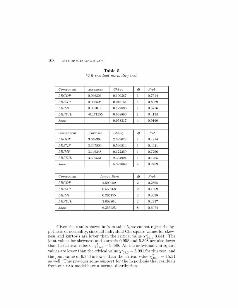
Table 5VAR residual normality test

Component Skewness Chi-sq df Prob.

LRGDP 0.066306 0.100387 1 0.7514

LREXP 0.026598 0.016154 1 0.8989

LRIMP 0.087018 0.172896 1 0.6776

LRFDIL -0.171155 0.668880 1 0.4134

Joint 0.958317 4 0.9160

Component Kurtosis Chi-sq df Prob.

LRGDP 3.648368 2.399672 1 0.1214

LREXP 3.307800 0.540814 1 0.4621

LRIMP 3.146348 0.122259 1 0.7266

LRFDIL 3.639561 2.334924 1 0.1265

Joint 5.397669 4 0.2489

Component Jarque-Bera df Prob.

LRGDP 2.500059 2 0.2865

LREXP 0.556968 2 0.7569

LRIMP 0.295155 2 0.8628

LRFDIL 3.003804 2 0.2227

Joint 6.355985 8 0.6074

Given the results shown in from table 5, we cannot reject the hy-pothesis of normality, since all individual Chi-square values for skew-ness and kurtosis are lower than the critical value χ2

.05,1 3.841. Thejoint values for skewness and kurtosis 0.958 and 5.398 are also lowerthan the critical value of χ2

.05,4 = 9.488. All the individual Chi-square

values are lower than the critical value χ2.05,2 = 5.991 for this test, and

the joint value of 6.356 is lower than the critical value χ2.05,8 = 15.51

as well. This provides some support for the hypothesis that residualsfrom our VAR model have a normal distribution.


Table 6 shows that we cannot reject the null hypothesis of noautocorrelation up to lag 12, since the values of the LM-Statistics forthe lag order of 1, 2, 3, 4, . . . 12, are all lower than the critical valueχ2

0.1,16 = 32 at 0.01 and 16 degrees of freedom.

Table 6VAR residual serial colrrelation LM test

Lags LM-Stat Probabilities from

Chi-square with 16

degrees of freedom

1 12.39986 0.7160

2 26.56133 0.0466

3 26.06180 0.0532

4 31.40808 0.0119

5 18.84123 0.2770

6 11.77191 0.7595

7 12.34180 0.7201

8 18.60542 0.2897

9 8.187881 0.9431

10 15.09080 0.5180

11 17.98524 0.3248

12 8.330402 0.9384

To test the long-run cointegration relationship between the fourtime series, we carried out the Johansen (1995) cointegration test.In order to do so, we first choose the appropriate lag criteria for thecointegration test. The results of the VAR order selection are given intable 7.

The FPE test and the AIC, SC and HQ Criteria confirm the selec-tion of a lag order of 1. With this information, we test for cointegra-tion among the four variables. The test results, reported in table 8,indicate that the four series are cointegrated. That is, there is somelong-run equilibrium relationship between the variables.

Since we can affirm the existence of cointegration within the fourseries, we continue to the next step, testing the causality relationships


between them. In order to find the causality between these four timeseries, we apply the Granger causality/Block exogeneity Wald test(Enders, 2003). This test detects whether the lags of one variable canGranger-cause any other variables in the VAR system. It tests bilat-erally whether the lags of the excluded variable affect the endogenousvariable. The null hypothesis is the following: all the lagged coeffi-cients of one variable can be excluded from each equation in the VAR

system. In table 9, “All” means: a joint test that the lags of all othervariables affect the endogenous variable.

Table 7Test for lag length criteria of the cointegration test

Lag LogL LR FPE AIC SC HQ

0 1.982275 NA 2.07e-05 0.563226 1.424048 0.913040

1 1016.661 1818.906 7.77e-12* -14.23202* -13.02687* -13.74228*

2 1024.950 14.36752 8.74e-12 -14.11778 -12.56830 -13.48812

3 1045.217 33.92857* 8.25e-12 -14.18100 -12.28719 -13.41141

Note: *indicates lag order selected by the criteria.

Table 8Johansen cointegration test with optimal lag length of 1

(trace and maximum eigenvalue)

Hypothesized

no. of CE(s)

Eigenvalue Trace

statistic

5 Percent

critical value

Prob**

critical value

None* 0.482521 120.7216 40.17493 0.0000

At most 1* 0.142062 31.12656 21.27596 0.0059

At most 2 0.072186 10.28816 12.32090 0.1070

At most 3 0.000724 0.098532 4.129906 0.7963

Trace test indicates 2 cointegrating equation(s) at the 5% level

* denotes rejection of the hypothesis at the 5% level

** MacKinnon-Haug-Michelis p-values

Hypothesized

no. of CE(s)

Eigenvalue Max-Eigen

Statistic

5 Percent

critical value

Prob**

None* 0.482521 89.59502 24.15921 0.0000


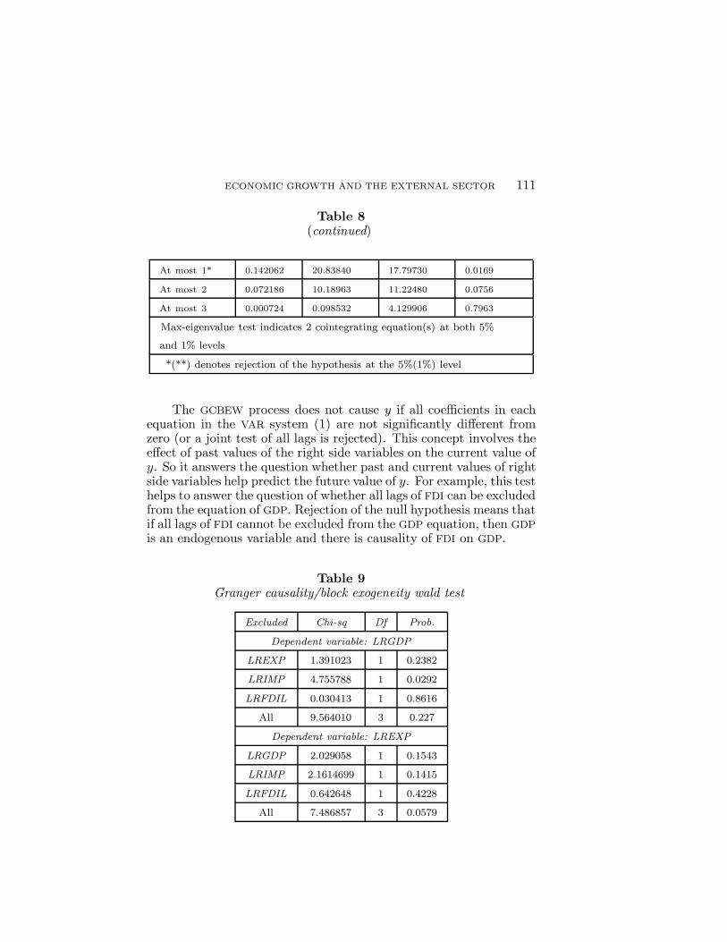
Table 8(continued)

At most 1* 0.142062 20.83840 17.79730 0.0169

At most 2 0.072186 10.18963 11.22480 0.0756

At most 3 0.000724 0.098532 4.129906 0.7963

Max-eigenvalue test indicates 2 cointegrating equation(s) at both 5%

and 1% levels

*(**) denotes rejection of the hypothesis at the 5%(1%) level

The GCBEW process does not cause y if all coefficients in eachequation in the VAR system (1) are not significantly different fromzero (or a joint test of all lags is rejected). This concept involves theeffect of past values of the right side variables on the current value ofy. So it answers the question whether past and current values of rightside variables help predict the future value of y. For example, this testhelps to answer the question of whether all lags of FDI can be excludedfrom the equation of GDP. Rejection of the null hypothesis means thatif all lags of FDI cannot be excluded from the GDP equation, then GDP

is an endogenous variable and there is causality of FDI on GDP.

Table 9Granger causality/block exogeneity wald test

Excluded Chi-sq Df Prob.

Dependent variable: LRGDP

LREXP 1.391023 1 0.2382

LRIMP 4.755788 1 0.0292

LRFDIL 0.030413 1 0.8616

All 9.564010 3 0.227

Dependent variable: LREXP

LRGDP 2.029058 1 0.1543

LRIMP 2.1614699 1 0.1415

LRFDIL 0.642648 1 0.4228

All 7.486857 3 0.0579


Table 9(continued)

Excluded Chi-sq Df Prob.

Dependent variable: LRIMP

LRGDP 4.121237 1 0.0423

LREXP 0.353790 1 0.5520

LRFDIL 0.354947 1 0.5513

All 6.370004 3 0.0949

Dependent variable: LRFDIL

LRGDP 4.329272 1 0.0375

LREXP 13.08574 1 0.0003

LRIMP 15.03986 1 0.0001

All 18.461 3 0.000

Table 9 reports the results from the GCBEW test and includesfour parts. The first part reports the result of testing that showswhether we can exclude each variable from the equation of LRGDP.Similarly, the next parts report the results of testing for the equationof LREXP, LRIMP and LRFDIL respectively. Each part of tableincludes four columns. The first column lists the variables that willbe excluded from the equation. The next columns are the value ofthe Chi-square test, degrees of freedom and P -value. The last row ineach part of the table reports the joint statistics of the three variablesexcluded from the equation.

In the first part of the table, which corresponds to the LRGDPequation, the second column shows that the Chi-squares for LREXP,LRIMP and LRFDIL are respectively 1.3910, 4.7558 and 0.0304.Thus, only one of the Chi-squares is greater than χ2

.01,1 = 2.706.Therefore, we can only reject the null hypothesis in one case, and con-clude that there is causality of LRIMP on LRGDP. This is confirmedby the fact that the joint Chi-square is 9.5640 > χ2

.05,3 = 7.815. Thisresult supports the imports-compression hypothesis. The correspond-ing values for LREXP and LRFDIL are less than χ2

.05,1 = 3.841, andso we cannot reject the null hypothesis in either cases, and can con-clude that there is no causality of LREXP and LRFDIL on LRGDP.

In the second part of Table 9, which corresponds to the LREXPequation, the second column shows that the respective Chi-squares


for LRGDP, LRIMP and LRDFIL are 2.0291, 2.1615 and 0.6426.None are greater than χ2

.05,1 = 3.84, and so we can’t reject the nullhypothesis in all cases, and conclude that there is no causality ofLRGDP, LRIMP or LRFDIL on LREXP. This is confirmed by thefact that the joint Chi-square is 7.4869 < χ2

.05,3 = 7.815.In the third part of the table, which corresponds to the LRIMP

equation, the second column shows that the respective Chi-squaresfor LRGDP, LREXP and LRFDIL are 4.1212, 0.3538 and 0.3549.The corresponding values for LREXP and LRFDIL are less thanthe critical value χ2

.05,1 = 3.841 and thus we cannot reject the nullhypothesis in those two cases, so we conclude that LRIMP is notcaused by LREXP or LRFDIL. However the corresponding value forLRGDP, 4.1212, is greater than the critical value χ2

.05,1 = 3.841,and therefore we conclude that LRGDP causes LRIMP. This assev-eration is confirmed by the fact that the joint Chi-square is 6.3700> χ2

.0.10,3 = 6.251In the fourth part of table 9, which corresponds to the LRFDIL

equation, the second column shows that the respective Chi-squares forLRGDP, LREXP and LRIMP are 4.3293, 13.0857 and 15.0399. Thecorresponding values for LRGDP, LREXP and LRIMP are greaterthan the critical value of χ2

.0.05,1 = 3.841. Thus we reject the nullhypothesis that LRGDP, LREXP and LRIMP do not cause LRFDIL;and we conclude that LRGDP, LREXP and LRIMP cause LRFDIL.This result is confirmed by the joint Chi-sq is 18.461 > χ2

.0.10,3 =6.251.

In summary:

1. We reject the null hypothesis of excluding LRIMP from LRGDPequation at a 0.05 significance level. This suggests that LRIMPcauses LRGDP.

2. We cannot reject the null hypothesis of excluding LRGDP, LRIMPand LRGDP from LREXP equation at a 0.05 significance level,suggesting that they do not cause LREXP.

3. We fail to reject the null hypothesis of excluding LREXP andLRFDIL from LRIMP equation at a 0.05 significance level. Thissuggests that LREXP and LRFDIL do not cause LRIMP. How-ever, we reject the null hypothesis of excluding LRGDP fromLRIMP equation at a 0.05 significance level, suggesting thatLRGDP does cause LRIMP.

4. We reject the null hypothesis of excluding LRGDP, LREXP and


LRIMP from LRFDIL equation at a 0.10 significance level, sug-gesting that all three variables do cause LRFDIL.

This test provides some evidence to believe that there is onebidirectional causality, between LRGDP and LRIMP; and three uni-directional causalities, those of LRGDP, LREXP, and LRIMP onLRFDIL.

Diagram 1Direction of causalities according to the GCBEW test

The GCBEW test provides information about the direction of theimpact, not the relative importance of variables that simultaneouslyinfluence each other. For instance, it is unclear whether or not theimpact of LREXP is stronger than that of LRGDP on LRFDIL. Toanswer these questions, we analyze the impulse-response function andthe variance decomposition (Shin and Pesaran, 1998).

4.2. Impulse-response analysis

Impulse response analysis traces the response of current and futurevalues of each of the variables to a one-unit increase (or to a one-standard deviation increase, when the scale matters) in the currentvalue of one of the VAR errors, assuming that this error returns to


zero in subsequent periods and that all other errors are equal to zero.Changing one error while retaining the others constant makes mostsense when the errors are uncorrelated across equations, so impulseresponses are typically calculated for recursive and structural VARs.

Figure 5 shows the generalized asymptotic impulse response func-tion. It includes 16 small figures, which are denoted figure 5.1, figure5.2, and so forth. Each small figure illustrates the dynamic responseof each target variable (LRGDP, LREXP, LRIMP and LRFDIL) toa one-standard-deviation shock on itself and other variables. In eachsmall figure, the horizontal axis presents ten quarters following theshock. The vertical axis measures the quarterly impact of the shockon each endogenous variable.

Figure 5.1 presents the long-run positive effect of a shock toLRGDP on LRGDP. This shock has a short- and long-run positiveeffect on LRGDP. Figure 5.2 shows that a shock to LREXP has nosignificant effect on LRGDP. Figure 5.3 shows that a shock on LRIMPhas a negative effect on LRGDP. Figure 5.4 shows that a shock toLRFDIL has no significant effect on LRGDP. These effects do notconflict with the GCBEW test.

Figure 5.5 suggests that in the long run, a shock on LRGDPhas a small significant positive effect on LREXP. Figure 5.6 suggeststhat LREXP has a positive effect on LREXP, as expected. Figure5.7 shows a significant effect of LRIMP on LREXP and Figure 5.8shows no significant effect of LRFDIL on LREXP. These results partlyconflict with the GCBEW test, specifically with respect to the effectof LRGDP on LREXP.

Figure 5.9 and 5.10 show the responses of LRIMP to shocks inLRGDP and LREXP; the shocks have a positive permanent signifi-cant effect on LRIMP. Figure 5.11 suggests that LRIMP has a posi-tive effect on LRIMP, as expected. Figure 5.12 shows no significanteffect of a shock in RDFIL on LRIMP. These results conflict withthe GCBEW test, specifically with respect of the effect of LREXP onLRIMP.

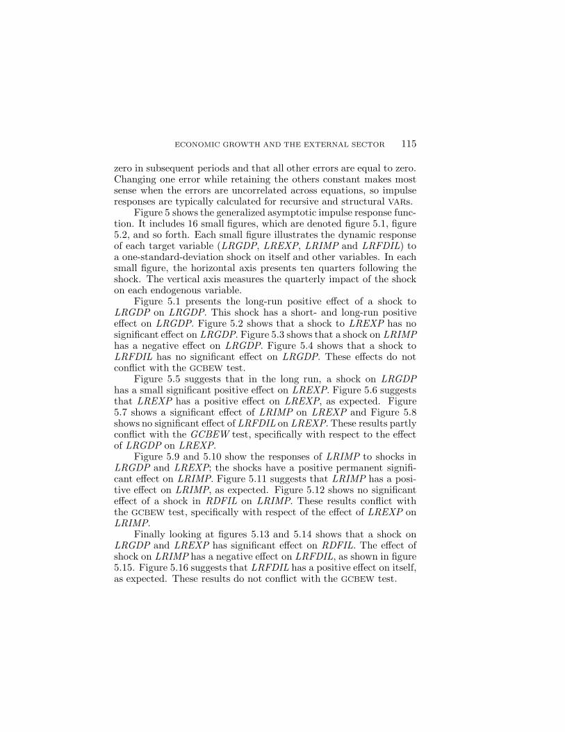
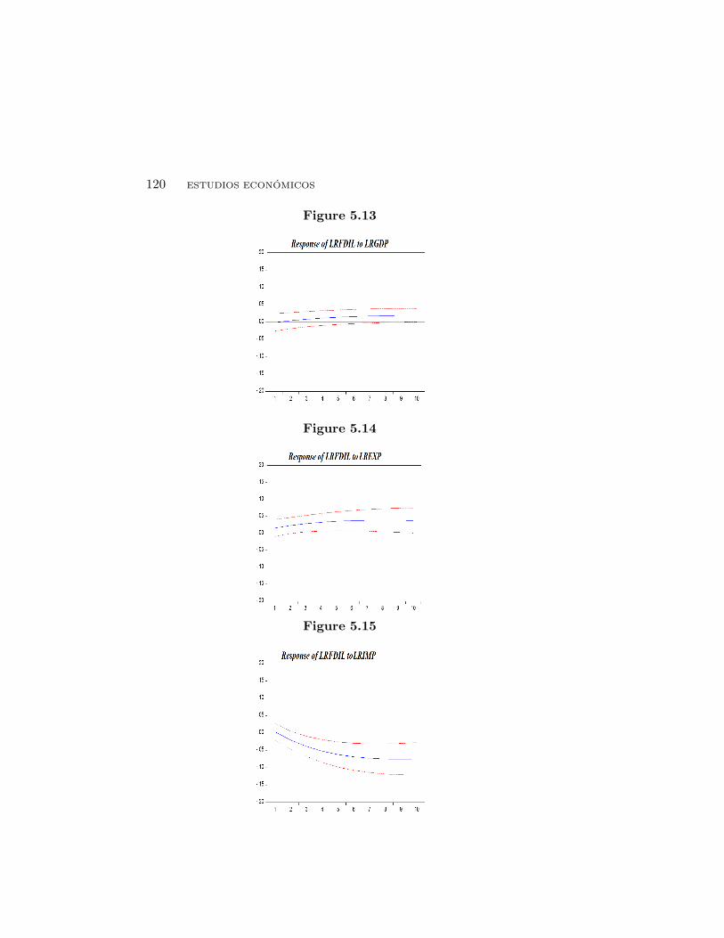
Finally looking at figures 5.13 and 5.14 shows that a shock onLRGDP and LREXP has significant effect on RDFIL. The effect ofshock on LRIMP has a negative effect on LRFDIL, as shown in figure5.15. Figure 5.16 suggests that LRFDIL has a positive effect on itself,as expected. These results do not conflict with the GCBEW test.


Figure 5.1

Figure 5.2

Figure 5.3


Figure 5.4

Figure 5.5

Figure 5.6


Figure 5.7

Figure 5.8

Figure 5.9


Figure 5.10

Figure 5.11

Figure 5.12


Figure 5.13

Figure 5.14

Figure 5.15


Figure 5.16

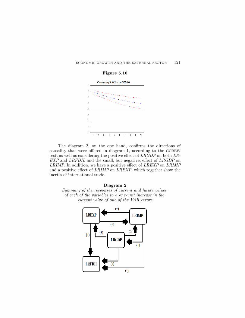
The diagram 2, on the one hand, confirms the directions ofcausality that were offered in diagram 1, according to the GCBEW

test, as well as considering the positive effect of LRGDP on both LR-EXP and LRFDIL and the small, but negative, effect of LRGDP onLRIMP. In addition, we have a positive effect of LREXP on LRIMPand a positive effect of LRIMP on LREXP, which together show theinertia of international trade.

Diagram 2Summary of the responses of current and future valuesof each of the variables to a one-unit increase in the

current value of one of the VAR errors


4.3. Variance decomposition

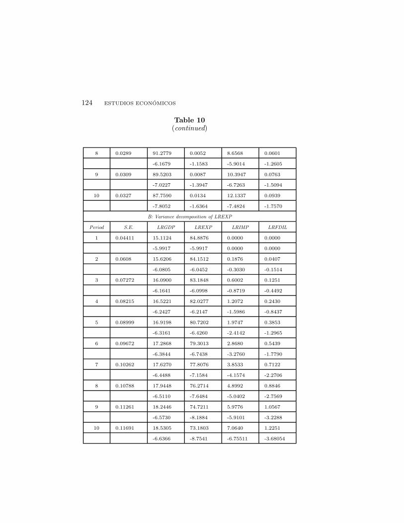
Variance decomposition (or forecast error variance decomposition)indicates the amount of information each variable contributes to theother variables in a VAR model (Enders, 2003). It tells us how muchof a change in a variable is due to its own shock and how much dueto shocks to other variables. In the short run most of the variationis due to a shock of its own, but as the effect of the lagged variablesstarts kicking in, the percentage of the effect of other shocks increasesover time. Therefore, the variance decomposition defines the relativeimportance of each random shock in affecting the variables in theVAR. Table 10 includes 4 individual tables, one for each variable.The standard errors are given below the respective coefficient.

Looking at table 10-A, in the short run (that is, three quar-ters) a shock to LRGDP accounts for 98.77% of the fluctuation inLRGDP (own shock); a shock to LREXP can cause 0.00% fluctua-tion in LRGDP (not statistically significant). A shock to LRIMP cancause a 1.22% fluctuation in LRGDP (not statistically significant) andLRFDI a 0.01% fluctuation in LRGDP (not statistically significant).

In the long run (10 quarters), a shock to GDP accounts for 87.76%of fluctuation in LRGDP, LREXP for 0.134% (not statistically sig-nificant), LRIMP 12.13% (statistically significant) and LRFDIL for0.09% (not statistically significant). Therefore, in the short run, noneof the variables have a statistically significant effect on LRGDP, andin the long run, only LRIMP does.

Looking at table 10-B, in the short run, a shock to LREXP ac-counts for a 83.18% fluctuation in LREXP (own shock), a shock toLRGDP causes a 16.09% fluctuation in LREXP (statistically signifi-cant). A shock to LRIMP causes a 0.60% fluctuation in LREXP (notstatistically significant) and LRFIL a 0.13% fluctuation in LREXP(not statistically significant).

In the long run, a shock to LREXP accounts for 73.18%, LRGDPto 18.53% (statistically significant), LRIMP 7.06% (not statisticallysignificant) and LRFDIL 1.23% (not statistically significant). There-fore, in the short and long run, only LRGDP has a statistically im-portant effect on LREXP.

Table 10-C shows that in the short run a shock to LRIMP ac-counts for 70.59% fluctuation in LRIMP (own shock), a shock toLRGDP can cause 7.09% fluctuation in LRIMP (statistically signif-icant). A shock to LREXP can cause 22.25% fluctuation in LRIMP(statistically significant) and LRFIL a 0.07% fluctuation in LRIMP(not statistically significant).


In the long run, a shock to LRIMP accounts for 64.65%, LRGDPto 10.85% (statistically significant), LREXP 23.79% (statistically sig-nificant) and LRFDIL 0.71% (not statistically significant). Therefore,in the short and long run, only LRGDP and LREXP have a statisti-cally important effect on LRIMP.

Looking at table 10-D, in the short run, a shock to LRFDILaccounts for 93.41% fluctuation in LRFDIL (own shock). A shockto LRGDP can cause 0.15% fluctuation in LRFDIL (not statisti-cally significant); a shock to LREXP can cause 2.89% fluctuation inLRFDIL (not statistically significant) and LRIMP a 3.54% fluctua-tion in LRFDIL (not statistically significant. In the long run, a shockto LRFDIL accounts for 64.00%, LRGDP to 1.48% (not statisticallysignificant), LREXP 8.06% (not statistically significant) and LRIMP25.46% (statistically significant). Therefore, in the short run, none ofthe variables have a statistically significant effect on LRFDIL, and inthe long run, only LRIMP has a statistically important effect on it.

Table 10Variance decomposition

A: Variance decomposition of LRGDP

Period S.E. LRGDP LREXP LRIMP LRFDIL

1 0.0100 100.0000 0.0000 0.0000 0.0000

0.0000 0.0000 0.0000 0.0000

2 0.0141 99.5995 0.0000 0.3986 0.0018

-0.4282 -0.0553 -0.4050 -0.0593

3 0.0173 98.7705 0.0000 1.2234 0.0061

-1.2156 -0.1676 -1.1529 -0.1810

4 0.0201 97.6170 0.0001 2.3702 0.0127

-2.1851 -0.3215 -2.0774 -0.3492

5 0.0225 96.2265 0.0004 3.7515 0.0216

-3.2209 -0.5053 -3.0683 -0.5508

6 0.0248 94.6705 0.0012 5.2957 0.0326

-4.2530 -0.7100 -4.0583 -0.7753

7 0.0269 93.0061 0.0027 6.9457 0.0455

-5.2420 -0.9291 -5.0092 -1.0141


Table 10(continued)

8 0.0289 91.2779 0.0052 8.6568 0.0601

-6.1679 -1.1583 -5.9014 -1.2605

9 0.0309 89.5203 0.0087 10.3947 0.0763

-7.0227 -1.3947 -6.7263 -1.5094

10 0.0327 87.7590 0.0134 12.1337 0.0939

-7.8052 -1.6364 -7.4824 -1.7570

B: Variance decomposition of LREXP


1 0.04411 15.1124 84.8876 0.0000 0.0000

-5.9917 -5.9917 0.0000 0.0000

2 0.0608 15.6206 84.1512 0.1876 0.0407

-6.0805 -6.0452 -0.3030 -0.1514

3 0.07272 16.0900 83.1848 0.6002 0.1251

-6.1641 -6.0998 -0.8719 -0.4492

4 0.08215 16.5221 82.0277 1.2072 0.2430

-6.2427 -6.2147 -1.5986 -0.8437

5 0.08999 16.9198 80.7202 1.9747 0.3853

-6.3161 -6.4260 -2.4142 -1.2965

6 0.09672 17.2868 79.3013 2.8680 0.5439

-6.3844 -6.7438 -3.2760 -1.7790

7 0.10262 17.6270 77.8076 3.8533 0.7122

-6.4488 -7.1584 -4.1574 -2.2706

8 0.10788 17.9448 76.2714 4.8992 0.8846

-6.5110 -7.6484 -5.0402 -2.7569

9 0.11261 18.2446 74.7211 5.9776 1.0567

-6.5730 -8.1884 -5.9101 -3.2288

10 0.11691 18.5305 73.1803 7.0640 1.2251

-6.6366 -8.7541 -6.75511 -3.68054


Table 10(continued)

C: Variance decomposition of LRIMP


1 0.0463 5.9557 21.0369 73.0074 0.0000

-4.8799 -5.7367 -6.6593 0.0000

2 0.0636 6.5252 21.7012 71.7510 0.0226

-4.9124 -5.8766 -6.6356 -0.1195

3 0.0759 7.0899 22.2494 70.5909 0.0699

-4.9608 -6.2784 -7.0355 -0.3662

4 0.0854 7.6483 22.6930 69.5223 0.1364

-5.0218 -6.8297 -7.7025 -0.7062

5 0.0933 8.1997 23.0439 68.5389 0.2175

-5.0924 -7.4455 -8.4910 -1.1084

6 0.0999 8.7437 23.3139 67.6337 0.3088

-5.1697 -8.0725 -9.3027 -1.5475

7 0.1055 9.2803 23.5139 66.7990 0.4068

-5.2521 -8.6812 -10.0822 -2.0037

8 0.1105 9.8098 23.6542 66.0275 0.5085

-5.3384 -9.2567 -10.8021 -2.4630

9 0.1149 10.3328 23.7439 65.3118 0.6115

-5.4279 -9.7921 -11.4517 -2.9151

10 0.1187 10.8498 23.7914 64.6450 0.7138

-5.5204 -10.2855 -12.0292 -3.3533

D: Variance decomposition of LRIMP


1 0.1479 0.0034 1.1334 0.0409 98.8223

-0.9559 -2.0541 -1.1617 -2.6277

2 0.1997 0.0453 1.9660 1.1147 96.8741

-0.9037 -2.4161 -1.5629 -3.0759


Table 10(continued)

3 0.2358 0.1534 2.8929 3.5426 93.4111

-0.9159 -2.7837 -2.8537 -4.1227

4 0.2646 0.3083 3.8340 6.7632 89.0945

-0.9716 -3.1786 -4.3474 -5.5358

5 0.2890 0.4918 4.7346 10.3160 84.4575

-1.0506 -3.6060 -5.7983 -7.0112

6 0.3103 0.6900 5.5641 13.8773 79.8685

-1.1399 -4.0569 -7.0934 -8.3536

7 0.3292 0.8931 6.3099 17.2482 75.5488

-1.2325 -4.5195 -8.1948 -9.4818

8 0.3460 1.0949 6.9704 20.3235 71.6113

-1.3252 -4.9851 -9.1074 -10.3845

9 0.3610 1.2916 7.5502 23.0610 68.0972

-1.4168 -5.4491 -9.8554 -11.0838

10 0.3743 1.4816 8.0570 25.4569 65.0046

-1.5068 -5.9089 -10.4690 -11.6131

From the GCBEW test, the impulse-response analysis and thevariance decomposition analysis, we can conclude the following:

• All three indicate that FDI has no effect on GDP growth or inter-national trade.

• All three indicate the existence of bidirectional effects betweenimports and GDP and of a unidirectional effect of imports on FDI

(although the sign is contradictory).

• Impulse-response analysis and variance decomposition coincide inshowing that GDP growth has a positive effect on exports.

• GCBEW test and the variance decomposition analysis establish pos-itive effects of exports and GDP on FDI.


• We find no evidence of the export-led growth hypothesis.

4.4. Lessons for Mexico

The causal dynamics of foreign trade and investment magnitudes withrespect to economic growth are a particularly important topic for in-vestigation; especially in the case of Korea, which has often beentaken as an example to emulate due to the outstanding growth ratesof its economy in the last decades. Accepting the exports-led growthhypothesis for Korea would not be, necessarily, a justification for itsimplementation in Mexico, because, as we have seen, the effects oftrade on the rest of the economy may vary among countries, depend-ing on their initial conditions and the strength of their institutions.However, our findings show that, in the representative case of Ko-rea, economic growth responded to an internal logic and not to theincrease of exports.

From the 1980s, Mexico began a period of export substitution,during which manufacturing exports began to have a greater relativeimportance than oil (Villarreal, 2005). In parallel, the 1980s meanta decade of increased FDI for Mexico. The opening of the Mexicaneconomy to international competition has been intense since the sign-ing of NAFTA in 1994. However, none of these policies have led to highlevels of economic growth for Mexico.

The final objective of export promotion policies should not besimply to increase exports, but rather, to achieve higher economicgrowth rates. The mere opening of a country does not guaranteethe creation of a productive sector: productive abilities are createdinternally. Thus, despite the importance of the external sector, as,for instance, a signaling mechanism for those firms to improve theircompetitiveness; policy makers should not just focus on an increaseof exports. As we have seen, even in the case of Korea, we must becautious about the effect of exports on economic growth.

We should properly understand the developmental models thatMexican policy makers take as a reference. If, as is claimed in thispaper, it is the case that exports and FDI are not the causes of Ko-rean economic growth, we should consider possibly reorienting theMexican growth model. Instead of focusing on further boosting avery concentrated and highly productive external sector, policy mak-ers should consider the adoption of an industrial policy that createsproduction capabilities within the country, regardless of whether suchproduction is exported. Exports will come as a consequence of thisimprovement.


5. Conclusions

In this paper, we have made an empirical analysis of the economicgrowth in Korea between 1980 and 2015, in order to identify the po-tential relationships between relevant variables. In doing so, we haveimplemented a methodology similar to Nguyen (2011). Our econo-metric procedures include the unit root test of relevant series, lagstructure, the VAR diagnostic, the Johansen cointegration test, theGranger causality/Block exogeneity Wald test (GCBEW), an analy-sis of impulse response and analysis of variance decomposition. Oneof the main results of this paper is that, for the Korean case, GDP

growth cannot be explained by increased exports. We believe thatthis is an important result, since it not only confronts the export-led growth hypothesis for the Korean case, but also undermines theexport promotion agenda as a tool to promote Mexicos development.

The advantages of trade liberalization for economic growth anddevelopment have been broadly debated in the relevant literature. Upuntil the mid-1970s, import substitution policies prevailed in mostdeveloping countries. Since then the emphasis has shifted towardsexport promotion strategies in an effort to promote economic devel-opment. It was hoped that export expansion would lead to betterresource allocation, creating economies of scale and production effi-ciency through technological development, capital formation and em-ployment generation. The shift also included an increasing relianceon FDI. The results of imposing and implementing those policies inLatin America, Africa and some East European countries have beendisappointing.

The realities of Korea’s successful growth case teach us a lessonand suggest that we may have to unlearn some lessons that we havebeen taught, and that we need to reconsider the effectiveness of thetraditional laissez-faire approach as a tool to boost economic devel-opment. As the Korean experience shows, growth in exports and aliberal trade policy cannot be seen as silver bullets that promote de-velopment, but rather as parts of a complex mechanism that may wellexpand the benefits of a whole set of policies that push the industri-alization and economic growth of a country. These are the benefitsthat have been denied to Latin America by the multinational insti-tutions and economic orthodoxy that have dominated the region formore than three decades.


References

Ahmad, J. and S. Harnhirun. 1995. Unit roots and cointegration in estimating

causality between exports and economic growth: Empirical evidence fromthe ASEAN countries, Economic Letters, 49: 329-334.

Amsden, A.H. 1989. Asia’s Next Giant: South Korea and Late Industrialization,New York, Oxford University Press.

Awokuse. 2007. Causality between exports, imports and economic growth: Evi-dence from transition economies, Economic Letters, 94(3): 389-395.

Balassa, B. 1985. Exports, policy choices, and economic growth in developing

countries after the 1973 oil shock, Journal of Development Economics, 18:23-35.

Chang, H.J. 1994. The Political Economy of Industrial Policy, London, MacMil-lan Press Ltd.

Conference Board, The. 2015. The Conference Board Total Economy Database,New York.

Elder, J. and P.E. Kennedy. 2001. Testing For unit roots: What should students

be taught? The Journal of Economic Education, 32(2): 137-146.

Enders, W. 2003. Applied Econometric Time Series, Hoboken, NJ, Wiley.

Feder, G. 1983. On exports and economic growth, Journal of Development Eco-nomics, 12: 59-73.

Guerrero de Lizardi, C. 2006. Thirlwall’s Law with an emphasis on the ratio of

export/import income elasticities in Latin American economies during thetwentieth century, Estudios Economicos, 21(1): 23-44.

Haggard, S. 1990. Pathways from the Periphery: The Politics of Growth inNewly Industrializing Countries, London, Cornell University Press.

Henriques, I. and P. Sadorsky. 1996. Export-led growth or growth-driven ex-ports? The Canadian case, The Canadian Journal of Economics, 29(3):540-555.

Herzer, D. 2012. How does foreign direct investment really affect developingcountries’ growth? Review of International Economics, 20(2): 396-414.

Johansen, S. 1995. Likelihood-Based Inference in Cointegrated Vector Autore-gressive Models, Oxford, Oxford University Press.

Jung, W.S. and P.J. Marshall. 1985. Exports, growth and causality in developingcountries, Journal of Development Economics, 18(1): 1-12.

Krueger, A. 1979. Studies in the Modernization of the Republic of Korea, 1945-

1975: The Developmental Role of the Foreign Sector and Aid, Cambridge,Harvard University Press.

——–. 1980. Trade policy as an input to development, American EconomicReview, 70: 288-292.

Konya. L. 2004. Export-led growth, growth-driven export, both or none?Granger causality analysis on OECD countries, Applied Econometrics andInternational Development, 4(1): 73-97.

Liew, V.K.S. 2004. Which lag length selection criteria should we employ? Eco-nomics Bulletin, 3(33): 1-9.


Liu, X., C. Shu, and P. Sinclair. 2009. Trade, foreign investment and economicgrowth in Asian economies, Applied Economics, 41(13): 1603–1612.

Liu, X.; C. Wang and Y. Wei. 2001. Causal links between foreign direct invest-ment and trade in China, China Economic Review, 12: 190-202.

Lutkepohl, H. 2005. Introduction to Multiple Time Series Analysis, Berlin,Springer-Verlag.

Nguyen, H.T. 2011. Exports, imports, FDI and economic growth, Working Paper,No. 11-03, University of Colorado.

OECD. 2016a. Quarterly National Accounts (database), <http://.dx.doi.org/10.1787/data-00285-en> (accessed on 27 June 2016).

OECD. 2016b. Balance of Payments (database), <http://.dx.doi.org/10.1787/data-00285-en> (accessed on 27 June 2016).

Santos-Paulino, A. and A.P. Thirlwall. 2004. The impact of trade liberalisationon exports, imports and the balance of payments of developing countries,The Economic Journal, 114: 50-72.

Shin, Y. and H.M. Pesaran. 1998. Generalized impulse response analysis inlinear multivariate models, Economic Letters, 58: 17-29.

Shirazi, N.S. and T.A. Abdul-Manap. 2005. Export-led growth hypothesis: Fur-ther econometric evidence from South Asia, The Developing Economies,43(4): 472-488.

Tyler, W.G. 1981. Growth and export expansion in developing countries: someempirical evidence, Journal of Development Economies, 9(1): 121-130.

Villarreal, R. 2005. Industrializacion, competitividad y desequilibrio externo enMexico: un enfoque macroindustrial y financiero (1929, 2010), Mexico,Fondo de Cultura Economica.

Westphal, L. 1978. The Republic of Korea’s experience with export-led industrialdevelopment, World Development, 6(3): 347-382.

Woo-Cumings, M. 1999. The Developmental State, Ithaca, Cornell UniversityPress.

World Bank. 1987. World Development Report 1987, New York, Oxford Uni-versity Press.

——–. 1993. The East Asian Miracle. Economic Growth and Public Policy,World Bank Policy Research Report, Oxford University Press.

Zestos, G.K. and X. Tao. 2002. Trade and GDP growth: Causal relations in theUnited States and Canada, Southern Economic Journal, 68(4): 859-874.

Appendix

In order to see how robust our results are, we have run both standardAugmented Dickey-Fuller (ADF) and Dickey-Fuller for GeneralizedLeast Squares (DFGLS) tests. In both cases, we chose the maximumlag by Schwert criterion, 13. In the case of standard ADF, we reducedthe lag by one if the respective statistic had an absolute value smallerthan 1.6. In the case of DFGLS, the lag order is chosen according tothe NG-Perron sequential t method.

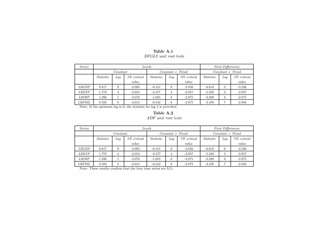
Table A.1

DFGLS unit root tests

Series Levels First Differences

Constant Constant + Trend Constant + Trend

Statistic Lag 5% critical Statistic Lag 5% critical Statistic Lag 5% critical

value value value

LRGDP 0.817 9 -2.005 -0.447 9 -2.856 -6.618 0 -3.536

LREXP 1.773 4 -2.054 -2.477 4 -2.957 -5.592 3 -2.957

LRIMP 1.296 1 -2.078 -1.685 8 -2.875 -3.389 8 -2.875

LRFDIL 0.593 8 -2.015 -0.542 8 -2.875 -3.476 7 -2.893

Note: If the optimum lag is 0, the statistic for lag 1 is provided.

Table A.2

ADF unit root tests

Series Levels First Differences

Constant Constant + Trend Constant + Trend

Statistic Lag 5% critical Statistic Lag 5% critical Statistic Lag 5% critical

value value value

LRGDP 0.817 9 -2.005 -0.447 9 -2.856 -6.618 0 -3.536

LREXP 1.773 4 -2.054 -2.477 4 -2.957 -5.592 3 -2.957

LRIMP 1.296 1 -2.078 -1.685 8 -2.875 -3.389 8 -2.875

LRFDIL 0.593 8 -2.015 -0.542 8 -2.875 -3.476 7 -2.893

Note: These results confirm that the four time series are I(1).

Documents

ECONOMIC GROWTH AND THE EXTERNAL SECTOR: EVIDENCE …