Embed Size (px)
Citation preview
Economic Disparities and Life Satisfactionin European Regions
M. Grazia Pittau Æ Roberto Zelli Æ Andrew Gelman
Accepted: 18 April 2009 / Published online: 28 April 2009� Springer Science+Business Media B.V. 2009
Abstract This paper investigates the role of economic variables in predicting regional
disparities in reported life satisfaction of European Union (EU) citizens. European sub-
national units (regions) are defined according to the first-level EU nomenclature of terri-
torial units. We use multilevel modeling to explicitly account for the hierarchical nature of
our data, respondents within regions and countries, and for understanding patterns of
variation within and between regions. Main findings are that personal income matters more
in poor regions than in rich regions, a pattern that still holds for regions within the same
country. Being unemployed is negatively associated with life satisfaction even after con-
trolled for income variation. Living in high unemployment regions does not alleviate the
unhappiness of being out of work. After controlling for individual characteristics and
modeling interactions, regional differences in life satisfaction still remain, confirming that
regional dimension is relevant for life satisfaction.
Keywords Life satisfaction � Regional disparities � Multilevel models
1 Introduction
Since Easterlin (1974), a blooming socio-economic literature on happiness has developed
ways of measuring happiness of individuals induced by life events, economic performances
and other ‘‘external’’ factors related to the area where people live (Frey and Stutzer 2002).
M. G. Pittau (&) � R. ZelliDSPSA, Sapienza Universita di Roma, Rome, Italye-mail: [email protected]; [email protected]
R. Zellie-mail: [email protected]
M. G. Pittau � A. GelmanDepartment of Statistics, Columbia University, New York, USA
A. Gelmane-mail: [email protected]
123
Soc Indic Res (2010) 96:339–361DOI 10.1007/s11205-009-9481-2
In this stream of literature, several studies have focused on the effects of socio-demo-
graphics (such as marital status, age and education) on individual well-being, while others
have focused on personal economic characteristics, mainly the level of income and the role
of being unemployed (Diener et al. 1993; Clark and Oswald 1994; Oswald 1997; Win-
kelmann and Winkelmann 1998).
A somewhat different perspective is the evaluation of the effects of macro-variables that
reflect the socio-economic environment where individuals live. Di Tella et al. (2003)
provide evidence that, after controlling for a wide set of individual characteristics, the
subjective well-being of Europeans is largely affected by levels and changes of country-
level macroeconomic variables, such as inflation, per capita GDP, unemployment rate and
social welfare state indicators. Alesina et al. (2004) and Graham and Felton (2006) address
the question of how income inequality affects individual well-being, finding different
results between developed and developing countries and also between United States and
Europe. Political arrangements also matter. The degree of trust and freedom of democratic
institutions (Layard 2005), as well as the degree of participating in direct democracy (Frey
and Stutzer 2000) seem to positively influence individual reported well-being.
Most of the analyses in the European Union (EU) have focused on the effects on
individual well-being of national economic indicators.1 On the other hand, it can be argued
that local rather than national macro-variables may influence the individual well-being to a
larger extent. The EU has devoted particular attention to subnational disparities that are
still wide both economically and socially. Their reduction is a target that has been made
explicit in the Treaty on EU and an increasing volume of the EU budget has been devolved
toward this objective (European Commission 2008).
Our paper focuses on the role of economic variables, both at individual and aggregate
level, in explaining observed subnational (regional) differences in life satisfaction of
Europeans.
Our understanding of the relation between economic variables and subjective well-
being is based on a strategy that refers to different levels of analysis. At the level of
individuals, we study to what extent personal characteristics make European citizens more
satisfied. Specifically, we concentrate on the role of personal income and employment
status. We want to determine to what extent personal income and employment status may
predict life satisfaction differently across European subnational units (‘‘regions,’’ defined
according to the first-level EU nomenclature of territorial units).
At aggregate level, we want to find out if the role of regional per capita GDP and
unemployment rate goes beyond the simple aggregation of individual effects, that is, for
example, do richer regions and poor regions may help predicting the individual well-being
in a different way?
Multilevel models provide a natural and suitable framework for accounting for these
different levels of variation, allowing us to understand the relation between income,
unemployment status and life satisfaction among individuals and regions simultaneously.
The paper is articulated as follows. In the next section we present the relevant char-
acteristics of the reported life satisfaction in our dataset in European countries and regions.
This section also sketches multilevel modeling and gives some details on the varying-
intercept and varying-slope model, which is our central fitted model. Section 3 reports the
empirical results of the fitted models. Throughout, we emphasize graphical summaries of
the results. Consistent with many other studies, we find that personal income is positively
1 A notable exception is the recent analysis of regional well-being in Europe by using European SocialSurvey data of Aslam and Corrado (2007).
340 M. G. Pittau et al.
123

associated to individual well-being and unemployment strongly deteriorates the subjective
life satisfaction, even controlling for the indirect effect of income loss.
Our main finding is that, on average, personal income matters more in poor regions than
in rich regions. Living in high unemployment regions does not alleviate the unhappiness of
being out of work. Finally, after controlling for individual characteristics and modeling
interactions, regional differences in life satisfaction still remain, confirming that regional
dimension is relevant for life satisfaction. Some concluding remarks are given in Sect. 4.
2 Data and Model Design
2.1 Measurement in the Eurobarometer Surveys
Research programs aimed to evaluate correlates and determinants of subjective well-being
rely, for the most part, on data collected from large surveys in which people are asked to
self-report their overall level of happiness and life satisfaction on a numerical scale. A
skeptical view on its use in economic and policy literature is expressed by Bertrand and
Mullainathan (2001) and Wilkinson (2007). This sort of survey is considered a fairly weak
technique for probing into people’s feelings, and more fine-grained self-reported tech-
niques, such as experience sampling or daily reconstruction, have been proposed as more
accurate tools to evaluate emotional recall (Kahneman and Krueger 2006).
Another concern is that cross-personal comparison is not possible: different people may
understand the concept of life satisfaction or happiness in different ways. In international
surveys, moreover, the terms ‘‘happiness’’ and ‘‘life satisfaction’’ have no precise equiv-
alent in some languages, reflecting cultural heterogeneity.
Beyond these measurement issues, life satisfaction is not the same as happiness: both
are broadly consistent measures of subjective well-being, but have to be considered sep-
arately. When asked how happy they are, people tend to consider the more volatile concept
of current emotional state, while life satisfaction is closer to the concept of an overall and
more stable living flourishing and actualizing the best potential within oneself. A person’s
subjective well-being includes both these emotive and cognitive judgments, and different
people weigh them differently. This explains how several nations, like Nigeria, report low
life satisfaction in the World Values Survey and at the same time high levels of happiness.
Even though questions on overall life satisfaction or happiness suffer from several
limitations, their use is widely recognized. A review of some of the arguments made in the
economic literature in favor of using survey ‘‘happiness data’’ is reported in Di Tella et al.
(2001) and Alesina et al. (2004). An evaluation of the reliability of the global judgment of
life satisfaction or happiness has been recently given by Krueger and Schkade (2007).
Apart from the fact that large surveys allow comparisons across many different groups of
people in terms of socio-economic characteristics, one argument is that responses to life
satisfaction questions have been found to be highly correlated with a variety of relevant
physical relations that can be thought of as describing true, internal happiness, as objective
physiological and medical criteria (e.g., electrical readings in the brain) or individual’s
emotional states (e.g., smiling frequency, sleep quality) or ratings made by friends. Fur-
thermore, when using representative population samples, idiosyncratic effects of recent
events that may affect the answers are likely to average out. Kahneman and Krueger (2006)
also note that respondents are not reluctant to answer life satisfaction or happiness ques-
tions. Overall, we acknowledge that available happiness data are flawed, perhaps more than
most economic data in several respects, but at any rate self-reported measurements tell us a
Economic Disparities and Life Satisfaction in European Regions 341
123
lot about the conditions under which different kinds of people are inclined to say that they
are satisfied or unsatisfied with life.
Data of our analysis are drawn from a series of repeated cross-sectional sample surveys,
the Eurobarometer surveys, collected and harmonized by ICPSR (Inter-university Con-
sortium for Political and Social Research) in the Mannheim Eurobarometer Trend File,
1970–2002 (Schmitt and Scholz 2005). The Eurobarometer surveys have been conducted
on behalf of the European Commission since the early seventies at least two times a year in
all member states on a representative sample of people aged 15 and over residing in the
EU. The Eurobarometer surveys include European countries only after their entrance to the
EU. The Eurobarometer series is designed to provide regular monitoring of the social and
political attitudes in the EU publics through specific trend questions. The Mannheim
Eurobarometer Trend File, a collaborative effort between the Mannheimer Zentrum fur
Europaische Sozialforschung and the Zentrum fur Umfragen, Methoden und Analysen,
combined the most important trend questions of the Eurobarometer surveys conducted
between 1970 and 2002. The file consisted of questions asked at least five times in standard
Eurobarometer surveys. Over 1.1 million respondents from a total of 15 EU member
nations were interviewed in these surveys.
Respondents were also asked for their overall satisfaction with life, as measured on a
four-point scale. The question usually asked is: ‘‘On the whole, are you very satisfied,
fairly satisfied, not very satisfied or not at all satisfied with the life you lead?.’’ Life
satisfaction questions were not asked in the 1996 surveys. The surveys also include a
similar question on the level of happiness, on a three-point scale, but this question was not
included in the most recent years. Demographic and other background information col-
lected include the respondents’ age, gender, and marital status, the number of people
residing in the household, the number of children under 15 in the household, respondent’s
age at completion of education, left-right political self-placement, occupation, religion,
income and region of residence.
2.2 Life Satisfaction in the European Regions
We first present an overall descriptive analysis of life satisfaction in Europe at national and
regional level. The Eurobarometer surveys have a code for the regions where individuals live.
We reclassify the Eurobarometer codes according to the most recent nomenclature of ter-
ritorial units for statistics (NUTS). We focus on the first level of the classification (NUTS1)
that divides the 15 European countries analyzed into a total of 70 subnational units.2 This
choice seems a reasonable compromise between the goal of investigating regional influences,
regional data availability and sample size. Previous empirical results of happiness equations
that make use of the Eurobarometer Surveys did cover the period from mid seventies to, at the
most, the year 1992 (Blanchflower and Oswald 2004; Di Tella et al. 2003). We analyze the
period 1992–2002, which is the last decade available in the Mannheim File.
In order to present a comprehensive picture, we treat the reported level of life satis-
faction as an ordinal measure from 1 for ‘‘not at all satisfied’’ to 4 for ‘‘very satisfied.’’
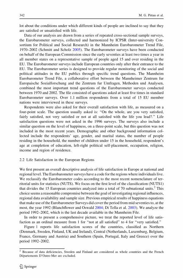
Figure 1 reports life satisfaction scores of the countries, classified as Northern
(Denmark, Sweden, Finland, UK and Ireland), Central (Netherlands, Luxemburg, Belgium,
France, Germany and Austria) and Southern (Spain, Portugal, Italy and Greece) over the
period 1992–2002.
2 Because of data deficiencies, Sweden and Finland are considered as whole countries and the FrenchDepartements D’Outre-Mer are excluded.
342 M. G. Pittau et al.
123
Northern countries were consistently more satisfied than the rest of Europe and were
also more stable over time. Denmark was by far the happiest country in the EU and its level
of life satisfaction was stable over time. Ireland seems to have had the most irregular
pattern, with a remarkable increase in 1997 followed by two evident declines, one in 1998
and the other in 2002. Regarding Central countries, Netherlands and Luxembourg reported
the highest levels of life satisfaction, while France reached the level of Germany after the
mid-1990. Southern countries showed the lowest levels of life satisfaction, but there was a
sizeable increase after 1998, especially Spain.
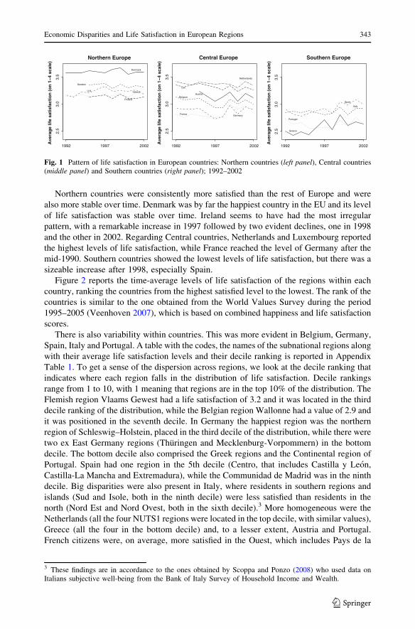
Figure 2 reports the time-average levels of life satisfaction of the regions within each
country, ranking the countries from the highest satisfied level to the lowest. The rank of the
countries is similar to the one obtained from the World Values Survey during the period
1995–2005 (Veenhoven 2007), which is based on combined happiness and life satisfaction
scores.
There is also variability within countries. This was more evident in Belgium, Germany,
Spain, Italy and Portugal. A table with the codes, the names of the subnational regions along
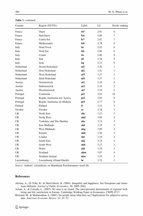
with their average life satisfaction levels and their decile ranking is reported in Appendix
Table 1. To get a sense of the dispersion across regions, we look at the decile ranking that
indicates where each region falls in the distribution of life satisfaction. Decile rankings
range from 1 to 10, with 1 meaning that regions are in the top 10% of the distribution. The
Flemish region Vlaams Gewest had a life satisfaction of 3.2 and it was located in the third
decile ranking of the distribution, while the Belgian region Wallonne had a value of 2.9 and
it was positioned in the seventh decile. In Germany the happiest region was the northern
region of Schleswig–Holstein, placed in the third decile of the distribution, while there were
two ex East Germany regions (Thuringen and Mecklenburg-Vorpommern) in the bottom
decile. The bottom decile also comprised the Greek regions and the Continental region of
Portugal. Spain had one region in the 5th decile (Centro, that includes Castilla y Leon,
Castilla-La Mancha and Extremadura), while the Communidad de Madrid was in the ninth
decile. Big disparities were also present in Italy, where residents in southern regions and
islands (Sud and Isole, both in the ninth decile) were less satisfied than residents in the
north (Nord Est and Nord Ovest, both in the sixth decile).3 More homogeneous were the
Netherlands (all the four NUTS1 regions were located in the top decile, with similar values),
Greece (all the four in the bottom decile) and, to a lesser extent, Austria and Portugal.
French citizens were, on average, more satisfied in the Ouest, which includes Pays de la
Northern Europe
Ave
rag
e lif
e sa
tisf
acti
on
(o
n 1
−4 s
cale
)
1992 1997 2002
2.5
3.0
3.5
Denmark
Sweden
U.K. Ireland
Finland
Central Europe
Ave
rag
e lif
e sa
tisf
acti
on
(o
n 1
−4 s
cale
)
1992 1997 2002
2.5
3.0
3.5
AustriaBelgium
FranceGermany
Lux
Netherlands
Southern Europe
Ave
rag
e lif
e sa
tisf
acti
on
(o
n 1
−4 s
cale
)
1992 1997 2002
2.5
3.0
3.5
Greece
Italy
Portugal
Spain
Fig. 1 Pattern of life satisfaction in European countries: Northern countries (left panel), Central countries(middle panel) and Southern countries (right panel); 1992–2002
3 These findings are in accordance to the ones obtained by Scoppa and Ponzo (2008) who used data onItalians subjective well-being from the Bank of Italy Survey of Household Income and Wealth.
Economic Disparities and Life Satisfaction in European Regions 343
123
Loire, Bretagne and Poitou-Charantes, positioned in the sixth decile, and less satisfied in the
Mediterranee region, positioned in the ninth decile ranking. UK regions were distributed
between the second and the fifth decile: Northern Ireland displayed the highest level of life
satisfaction (3.3, very similar to Ireland), with Scotland the lowest (3.1, similar to the
northern English regions, North East and North West). Regions where the capital city is
located usually reported levels of happiness among the lowest within their country. This was
the case for London, Berlin, Paris, Madrid, Vienna and Athens.
The observed variability across European regions motivates our choice to account for
both individual-and regional-level variation in a multilevel framework.
2.3 Multilevel Modeling
Multilevel modeling can be thought as linear or generalized linear regression in which the
parameters, the varying group coefficients, are given a probability model. Classical
regression can incorporate varying groups coefficients by including dummy variables, but
the main difference between multilevel and classical regression is in the modeling of the
variation between groups. The crucial multilevel modeling step is that the group coefficients
are themselves modelled (most simply a common distribution for the group coefficients or,
more generally, a regression model that includes group-level predictors). Multilevel models
can include group indicators (dummies) along with group-level predictors. As special cases
of multilevel models are the classical regression models. When the variation between
groups tend to zero, multilevel models collapse to complete-pooling models, while when the
Average life satisfaction (on 1−4 scale)2.5 3.0 3.5
Greece
Portugal
France
Italy
Germany
Spain
Belgium
Finland
Austria
United Kingdom
Ireland
Luxembourg
Sweden
Netherlands
Denmark
Fig. 2 Average life satisfaction in European regions on the period 1992–2002. The circles represent theEuropean NUTS1 subnational regions. Countries are ordered from the most to the least satisfied with life
344 M. G. Pittau et al.
123
variation between groups goes to infinity they reduce to the no-pooling model. Given
multilevel data, we can estimate the variation between groups. Therefore, there is no reason
(except for convenience) to accept estimates that arbitrarily set this parameter to one of
these two extreme values (Gelman and Hill 2007).
When the number of groups is large, there is typically enough information to accurately
estimate group-level variation from the data alone and, as a result, multilevel models gain
much beyond classical varying-coefficient models, that suffer from reduction in degrees of
freedom. Multilevel models, in this setting, estimate more accurately heterogeneous groups
in small samples, avoiding the problem of large standard error related to the smallness of
sample size in small area estimation procedures (Longford 2007).
There are two compelling reasons for using multilevel models to study the effects of
socio-economic conditions of Europeans on their level of life satisfaction.
First, multilevel models allows us to explicitly account for the hierarchical nature of our
data. We use, in fact, as predictors of life satisfaction variables both at individual and at
regional level coming, respectively, from survey data on individuals (Eurobarometer) and
national accounting data for regions and countries (Eurostat). Second, multilevel models also
let us estimate patterns of variation within and between regions simultaneously, by allowing
their intercepts, and eventually slopes, to vary (see Snijders and Bosker 1999, for a general
overview of multilevel models, and Gelman and Hill 2007, for the notation used here).
Since reported life satisfaction is intrinsically ordinal, the natural way to treat it in an
econometric model should be by ordered logit or probit equations. As discussed in Ferrer-i-
Carbonell and Frijters (2004) and Frey and Stutzer (2002), ordinality or cardinality of life
satisfaction scores makes little difference, so the use of ordered logit models or linear
models is not expected to change the substantive findings. To give grounds to this
hypothesis, we implement the ordered logit, and the easier to interpret linear regression for
modeling the determinants of satisfaction in life.
Whatever the choice of the selected functional form, our central model is a multilevel
varying-intercept and varying-slope model that estimates life satisfaction on individual
socio-demographic characteristics and regional variables. Considering for sake of sim-
plicity only one individual predictor, life satisfaction of individual i resident in region j can
be written as:4
yi�Nðaj½i� þ bj½i�xi; r2yÞ; i ¼ 1; . . .; n; ð1Þ
where y is the life satisfaction level, x is an individual-level predictor, as income, r2y is the
unexplained within-region variation and j[i] indexes the region j where person i resides.
The second step of the model, what makes it ‘‘multilevel,’’ is the simultaneous modeling
of the region-level intercepts aj and slopes bj as:
aj
bj
� ��N
la
lb
� �;
r2a qrarb
qrarb r2b
� �� �; for j ¼ 1; . . .; J
where la and lb are the means of the region intercepts and slopes respectively, ra and rb
their standard deviations and q the between-region correlation parameter.
A further step of the model is to add group-level predictors to improve inference for the
group coefficients aj and the varying slopes bj:
4 Without lacking of generality of the multilevel framework, we treat the outcome y as a continuousvariable. In case of generalized linear models, it is necessary to adapt model (1) to the logistic scale (Gelmanet al. 2008a, b).
Economic Disparities and Life Satisfaction in European Regions 345
123
aj�Nðca0 þ Ujc
a; r2aÞ; j ¼ 1; . . .; J ð2Þ
bj�Nðcb0 þ Ujc
b; r2bÞ; j ¼ 1; . . .; J ð3Þ
where U is a matrix of region-level predictors, ca the vector of coefficients for the region-
level regression (2) and cb the vector of coefficients for the region-level regression (3).
Group-level predictors not only are themselves of interest, but play a special role in the
multilevel context, since they may reduce the unexplained group-level variation, that are
the standard deviation ra and rb. Reduction of unexplained group-level variation can be
therefore interpreted as a measure of the importance of the predictor.
Since our model focuses on the effects of economic variables, we let the coefficients of
personal income and unemployment status vary by group (region). To control for demo-
graphic characteristics, we also consider additional variables whose coefficients are un-
modelled, as sex, age, marital status, education.
When we have multiple predictors, it is convenient to move to matrix notation in which
there are J groups, K individual-level predictors whose coefficients vary by group
(including the constant term), R individual-level predictors whose coefficients do not vary
by group and L predictors in the group-level regression (including the constant term):
yi�NðX0i b
0 þ XiBj½i�; r2yÞ; for i ¼ 1; . . .; n
Bj�NðMB;RBÞ; for j ¼ 1; . . .; J;ð4Þ
where X0 is the n 9 R matrix of individual predictors and b0 the vector of their unmodelled
regression coefficients; X is the n 9 K matrix of individual predictors (the first column is a
column of 1s) that have coefficients varying by groups and B is the J 9 K matrix of their
regression coefficients. Therefore, Bj[i] is the jth row of B, that is the vector representing the
intercept and the slope for the group that includes unit i. MB is a vector representing
the mean of the distribution of the varying-intercepts and varying-slopes and RB is the
covariance matrix.
We can extend model (4) to include group-level predictors:
yi�NðX0i b
0 þ XiBj½i�; r2yÞ; for i ¼ 1; . . .; n
Bj�NðUjG;RBÞ; for j ¼ 1; . . .; J;ð5Þ
where B is the J 9 K matrix of individual-level coefficients, U is the J 9 L matrix of
group-level predictors (including the constant term), and G is the L 9 K matrix of coef-
ficients for the group-level regression.
2.4 Regional Macroeconomic Variables as Group Predictors
The group-level predictors we include in our more structured model are macroeconomic
variables at the subnational level. The subnational variables are from Regio, the Eurostat’s
harmonized regional statistical database. Regio covers the main aspects of economic and
social life in the EU, classified up to the first three levels of the nomenclature of territorial
units (NUTS). National accounts aggregates at NUTS level are based on data from the
European System of Accounts ESA 1995, using an harmonized methodology, and were
calculated by Eurostat from 1995. On the other hand, as previously mentioned, life sat-
isfaction data are not available for 1996. Therefore, due to data availability in the Euro-
barometer surveys and in the European regional data set, we confine our modeling to the
346 M. G. Pittau et al.
123
1997–2002 period. The groups (the second level of the model) we refer to are 70 regions of
15 European countries at NUTS1, the first category of the nomenclature of territorial units.
The group-level predictors are regional per capita GDP and regional unemployment
rate. These two economic variables, along with the rate of inflation, have been most
thoroughly investigated and recognized as the most influential. On the first variable, Frey
and Stutzer (2002) report studies showing that life satisfaction and income are uncorrelated
over time within countries. Across countries, instead, they observe weak correlation once a
certain stage of income has been reached. They also document that higher levels of
unemployment reduce the average satisfaction with life, even after controlling for indi-
vidual unemployment status. The GDP per capita, instead, matters among European
countries, as shown in Di Tella et al. (2003), giving us a motivation to investigate these
relationships across European regions in further details.
Regional per capita income is the GDP per inhabitant at market prices converted to
national purchasing power standard to make a correction for different cost of living.
Unfortunately, Eurostat does not possess comparable regional price levels which would
have been enabled us to handle for regional differences in price levels within same
countries. Adjusting GDP per capita to national purchasing power has effects on data
dispersion since low incomes in poor regions tend to be partially counterbalanced by lower
costs of living (Pittau and Zelli 2006). Unemployment rates represent unemployed persons
as a percentage of the civilian labor force in each region.
3 Empirical Results
3.1 Influence of Individual Characteristics
We start fitting models that allow personal characteristics to predict life satisfaction within
each region, letting the intercepts aj vary across regions but keeping unmodeled the slopes
b’s, that is a special case of model (4) in which X is simply a vector of 1s. The inclusion of
a varying intercept captures region-to region variation that remains unexplained after
controlling for individual characteristics.
We estimate the model considering the linear and ordered logit specification.5 In
the linear model, life satisfaction outcome is treated as a continuous variable ranging from
1 to 4, while in the ordered logistic regression life satisfaction is considered as a four
categorical outcome.
Individual characteristics used as first-level predictors are: income level, employment
status, age, marital status, gender and education level.6 For other interesting characteristics,
like religion, number of children and political self-placement, we have too many missing
5 Estimates of the models are obtained by the lmer function in R (R Development Core Team 2006) and arebased on the restricted maximum likelihood procedure (REML). The REML procedure corrects thedownwards bias of the maximum likelihood estimator of variance components related to the lost of degreesof freedom in estimating the fixed effects. The name lmer stands for linear mixed effects in R but thefunction works also for generalized linear models. However some technical challenges exist in fittingmultinomial models in a multilevel framework. Therefore, for the ordered logit model we use the classicalno-pooling regression. The term ‘‘mixed effects’’ refers to random effects (coefficients that vary by group)and fixed effects (coefficient that do not vary) (Gelman and Hill 2007).6 As pointed out by, e.g., Di Tella et al. (2003) and Frey and Stutzer (2006), estimated effects should betreated with caution since some personal characteristics can be considered endogenous. Moreover ifunobserved personal traits influence reported life satisfaction, results suffer from potential bias.
Economic Disparities and Life Satisfaction in European Regions 347
123
observations to include them in the equation since for several years these variables have
not been collected. The Mannheim Trend File uses twelve income categories, making this
variable comparable across countries and over time. Income classes are expressed in
absolute values. Educational categories refer to the age when interviewers finished their
full-time education and are codified as: up to 15 years old, between 16 and 19 years old,
over 20. We exclude interviewers who responded ‘‘don’t know’’ or did not respond.
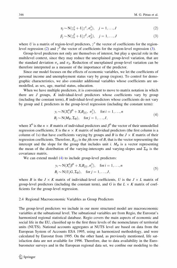
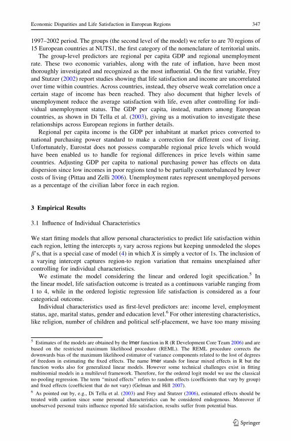
Figures 3 and 4 report the estimated coefficients for the individual characteristics in the
two different model specifications.7 Time indicator variables are included in the models.
The zeros correspond to the baseline categories for each categorical variable.
The influence of economic individual characteristics on life satisfaction are in accor-
dance to the main findings of Di Tella et al. (2003) on the Eurobarometer surveys in
coefficients of the linear model−0.10 −0.05 0.00 0.05 0.10 0.15 0.20
more 20 years16−19 years
less 15 yearsfemale
maleunemployed
retiredstudent
homeemployed
self−employedwidowed
separateddivorced
as marriedmarried
singleage/10 squared
age/10Income level 12Income level 11Income level 10
Income level 9Income level 8Income level 7Income level 6Income level 5Income level 4Income level 3Income level 2Income level 1
year 2002year 2001year 2000year 1999year 1998year 1997
Fig. 3 Estimated coefficients with relative ±2 standard errors of individual characteristics in the basic fittedmultilevel linear model with respondents nested within regions and countries (1997–2002)
7 Due to data availability in the European regional data set we use in models with more complex multilevelstructure, we report for coherence the results of the fitting for the period 1997–2002. However, we did notfind any significant difference when we use the Eurobarometer data expanding the period backward to 1992.Detailed results of the fitted models are available upon request from the authors.
348 M. G. Pittau et al.
123
previous years. The effects of income and unemployment status are substantial in both
specifications. In the linear models there are no significant differences with respect to first
income class until income level 4. But, for example, moving from the bottom class to the
upper income class (level 11) increases, ceteris paribus, the life satisfaction score by 0.11.
Interpreting the coefficients of the ordered logistic regression is not straightforward. Given
the estimated cutpoints, the baseline individual (who is a man of average age, with income
level 1, self-employed, single, who left school before 15 years old and interviewed in the
year 1997) has a probability of being ‘‘very satisfied’’ approximately equal to 2%, of being
‘‘fairly satisfied’’ equal to 62%, of being ‘‘not very satisfied’’ equal to 37% and being ‘‘not
at all satisfied’’ equal to 1%. If this man increases his income level until class 11 the
estimated probabilities change as follow: ‘‘very satisfied’’ to 3%, ‘‘fairly satisfied’’ to 88%,
‘‘not very satisfied’’ 9% and ‘‘not at all satisfied’’ to 0%. Regarding the employment status,
being unemployed has a negative and highly significant effect even though we are con-
trolling for income. Being unemployed with respect to being self-employed reduces by
0.05 life satisfaction level in the linear specification without accounting the eventual
coefficients of the ordered logit model−1.0 −0.5 0.0 0.5 1.0 1.5
more 20 years16−19 years
less 15 yearsfemale
maleunemployed
retiredstudent
homeemployed
self−employedwidowed
separateddivorced
as marriedmarried
singleage/10 squared
age/10Income level 12Income level 11Income level 10
Income level 9Income level 8Income level 7Income level 6Income level 5Income level 4Income level 3Income level 2Income level 1
year 2002year 2001year 2000year 1999year 1998year 1997
Fig. 4 Estimated coefficients with relative ±2 standard errors of individual characteristics in the basic fittedordered logistic model with respondents nested within regions and countries (1997–2002). The estimatedcutpoints and their standard errors are: c1|2 = -3.52 (0.11), c2|3 = -1.57 (0.10), c3|4 = 1.62 (0.10)
Economic Disparities and Life Satisfaction in European Regions 349
123
income loss. Again, the interpretation of the ordered logistic model has to be done referring
to a specific respondent. As an example, the probability of the baseline individual of being
‘‘very satisfied’’ if he becomes unemployed decreases from 2% to 0%, the probability of
being ‘‘fairly satisfied’’ goes down from 62% to 40%, while the probability of being ‘‘not
very satisfied’’ increases by 18 percentage points. His probability of being ‘‘not at all
satisfied’’ goes up from 1% to 5%.
Also for social and demographic characteristics our results confirm evidence of previous
literature. Life satisfaction increases with years of education. Women are, ceteris paribus,
more satisfied than men. Marital status appears to have a positive association on life
satisfaction for those who are in some form of relationship (married or as married) while it
has the most negative association for those who are separated or divorced. There is U-
shape pattern of happiness with age: happiness starts off relatively high in early adulthood,
then falls, reaching its minimum in middle age, and then rises after that age into old age, in
line with results obtained by Blanchflower and Oswald (2004).
Overall our findings confirm that associations with individual characteristics analyzed in
micro-econometric ‘‘happiness’’ regressions display similar structure across time and,
whatever the model specification, the fitted regressions display similar patterns. For a more
straightforward interpretation of the coefficients from now on we concentrate on the linear
specification.
3.2 Do Personal Income and Unemployment Status have a Common Effect
across Regions?
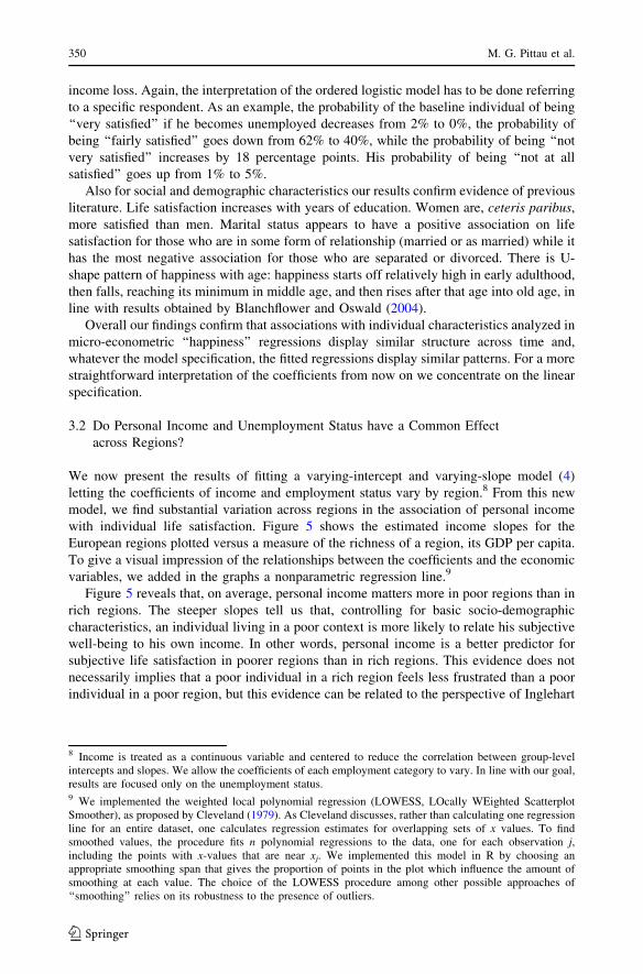
We now present the results of fitting a varying-intercept and varying-slope model (4)
letting the coefficients of income and employment status vary by region.8 From this new
model, we find substantial variation across regions in the association of personal income
with individual life satisfaction. Figure 5 shows the estimated income slopes for the
European regions plotted versus a measure of the richness of a region, its GDP per capita.
To give a visual impression of the relationships between the coefficients and the economic
variables, we added in the graphs a nonparametric regression line.9
Figure 5 reveals that, on average, personal income matters more in poor regions than in
rich regions. The steeper slopes tell us that, controlling for basic socio-demographic
characteristics, an individual living in a poor context is more likely to relate his subjective
well-being to his own income. In other words, personal income is a better predictor for
subjective life satisfaction in poorer regions than in rich regions. This evidence does not
necessarily implies that a poor individual in a rich region feels less frustrated than a poor
individual in a poor region, but this evidence can be related to the perspective of Inglehart
8 Income is treated as a continuous variable and centered to reduce the correlation between group-levelintercepts and slopes. We allow the coefficients of each employment category to vary. In line with our goal,results are focused only on the unemployment status.9 We implemented the weighted local polynomial regression (LOWESS, LOcally WEighted ScatterplotSmoother), as proposed by Cleveland (1979). As Cleveland discusses, rather than calculating one regressionline for an entire dataset, one calculates regression estimates for overlapping sets of x values. To findsmoothed values, the procedure fits n polynomial regressions to the data, one for each observation j,including the points with x-values that are near xj. We implemented this model in R by choosing anappropriate smoothing span that gives the proportion of points in the plot which influence the amount ofsmoothing at each value. The choice of the LOWESS procedure among other possible approaches of‘‘smoothing’’ relies on its robustness to the presence of outliers.
350 M. G. Pittau et al.
123
(1990) and other scholars of postmaterialism, with life satisfaction in rich societies more
related to non-materialistic issues.10
This pattern holds for almost all the countries for which we have enough regions,
confirming the variability between regions within the same country. From the multilevel
regression with varying intercepts and slopes, we display in Fig. 6, for a selection of
countries, life satisfaction as a function of individual income. In each graph, the three (or
four) lines represent the predicted values of life satisfaction as a function of income
categories for three or four representative regions within the country: a rich region (in
terms of per capita GDP), one or two middle income region and a (relatively) poor region.
For each region in the plot, the circles show the relative proportion of individuals in each
income category. Within the same country, we generally find a systematic pattern of the
within-region slopes, with the steepest slope in the poorest region and the shallowest slope
in the richest region: income is always positively correlated with life satisfaction, but it is a
weaker predictor in rich regions and a strong predictor in poor regions. This is true for
France, Italy and Spain. In United Kingdom, Northern Ireland is the only exception since
its slope is flatter than expected. Germany and Greece do not display such a clear pattern
since middle-income regions (Hessen for Germany and Kentriki Ellada for Greece) display
0.02
0.03
0.04
0.05
log of GDP per capita (purchasing power adjusted)
Inco
me
slop
es β
nuts
9.5 10.0 10.5
be1
be2
be3
dk
de1
de2
de3
de4de5
de6
de7
de8
de9
dea
deb
dec
deddee
def
deg
ie
gr1
gr2
gr3
gr4
es1
es2
es3es4
es5
es6
es7fr1
fr2
fr3
fr4
fr5fr6
fr7
fr8
itc
itd
ite
itfitg
nl1
nl2
nl3
nl4
at1at2
at3
pt1
pt2pt3
fi
se
ukc
ukd
ukeukf
ukg
ukh
ukiukj
ukk
ukl
ukm
ukn lu
Fig. 5 Estimated regional income slopes bj in the varying-intercept varying-slope regression model plottedversus regional log of GDP per capita, purchasing power adjusted, 2001. The regional income slopesmeasure the association of individual income with life satisfaction within each region. The horizontal linerepresents the European average of the slopes. The curve shows lowess fits (Cleveland 1979)
10 We thank the referee for having emphasized this point. Consistently, Gelman et al. (2008a, b) show howpatterns of income, religion, and voting in the U.S. are consistent with Inglehart’s post-materialismhypothesis.
Economic Disparities and Life Satisfaction in European Regions 351
123

2.6
2.8
3.0
3.2
3.4
United KingdomE
xpec
ted
life
satis
fact
ion
low middle high
London
Scotland
Wales
Northern Ireland
2.6
2.8
3.0
3.2
3.4
Spain
Exp
ecte
d lif
e sa
tisfa
ctio
n
low middle high
Comunidad de Madrid
EsteSur
2.6
2.8
3.0
3.2
3.4
Germany
Exp
ecte
d va
lue
of li
fe s
atis
fact
ion
low middle high
Hessen
Thuringen
Hamburg 2.6
2.8
3.0
3.2
3.4
ItalyE
xpec
ted
life
satis
fact
ion
low middle high
low middle high low middle high
Centro
Sud
Nord Est
2.6
2.8
3.0
3.2
3.4
France
Exp
ecte
d lif
e sa
tisfa
ctio
n
Ile de France
Est
Nord−Pas−de−Calais
2.6
2.8
3.0
3.2
3.4
Greece
Exp
ecte
d lif
e sa
tisfa
ctio
n
Voreia Ellada
Kentriki Ellada
Attiki
Fig. 6 Expected life satisfaction as a function of income categories, for a selection of European countries.For each country, the lines are based on the fitted varying-intercept and varying-slope linear model and referto a rich region, middle income regions and a poor region. The circles show the relative proportion ofindividuals in each income category in each region. The richest regions in terms of per capita GDP are:London (UK), Comunidad de Madrid (Spain), Hamburg (Germany), Nord Est (Italy), Ile de France (France),Attiki (Greece). Middle income regions are: Scotland and Northern Ireland (UK), Este (Spain), Hessen(Germany), Centro (Italy), Est (France), Kentriki Ellada (Greece). The poorest regions are: Wales (UK), Sur(Spain), Thuringen (Germany), Sud (Italy), Nord-Pas-de-Calais (France), Voreia Ellada (Greece)
352 M. G. Pittau et al.
123
the shallowest slope while the richest regions (Hamburg and Attiki) have the same slope as
the poorest regions (Thuringen and Voreia Ellada).
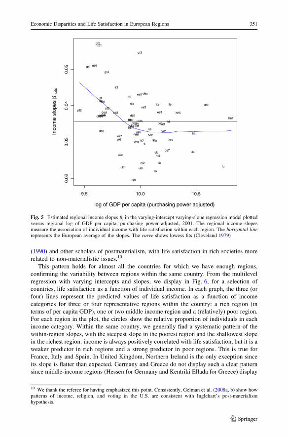
Figure 7 shows the estimated coefficients of model (4) associated with unemployment
status plotted versus the unemployment rate of the regions. The negative effect on life
satisfaction of being unemployed is strong in all regions (on average -0.22), with an
estimated variability of 0.11. These estimated values indicate that the self-proclaimed well-
being of an unemployment individual is much lower than the level of an employed indi-
vidual with similar characteristics in each region. Since we are controlling for all the
individual attributes, including individual income, these negative coefficients might be
interpreted as ‘‘pure’’ effects of being unemployed: unemployed people suffer from high
non-pecuniary costs beyond the expected drop in their income level.
According to a large body of economic literature of happiness (see, e.g., Frey and
Stutzer 2002; Clark 2003), an environment with a large portion of people out of work
should alleviate the unhappiness of being unemployed. When the reference group is the
European subnational region, this thesis is not supported by our data. As reported in Fig. 7,
unemployed regional coefficients do not reduce as regional unemployment rates increase.
This evidence does not necessarily mean that there is no social psychological effect of
being unemployed in an environment where the others are also unemployed, but our results
are not in line with this hypothesis when the reference group is the region.
−0.
4−
0.3
−0.
2−
0.1
Unemployment rates
Coe
ffici
ents
for
indi
vidu
al u
nem
ploy
men
t sta
tus
0% 10% 20%
be1
be2
be3
dkde1
de2
de3
de4
de5
de6
de7
de8
de9
dea
deb
dec
ded
deedef
deg
ie
gr1
gr2
gr3
gr4
es1
es2
es3
es4
es5
es6
es7fr1
fr2
fr3
fr4
fr5
fr6
fr7
fr8
itc
itd
ite
itf
itg
nl1
nl2
nl3
nl4
at1at2
at3
pt1
pt2
pt3
fi
se
ukc
ukd
uke
ukf
ukg
ukh
uki
ukj
ukk
ukl
ukm
ukn
lu
Fig. 7 Estimated regional coefficients bj for individual unemployment status in the varying-interceptvarying-slope regression model plotted versus regional unemployment rate, 2001. The regional coefficientsfor individual unemployment status measure the association of being unemployed with life satisfactionwithin each region. The horizontal line represents the European average of the slopes. The curve showslowess fits (Cleveland 1979)
Economic Disparities and Life Satisfaction in European Regions 353
123
To go beyond the visual impression of Figs. 5 and 7, we verify the detected relationship
by introducing GDP per capita and unemployment rate as contextual variables in the
second level of the multilevel model (5). We model income coefficients and unemploy-
ment coefficients as a function of per capita GDP and unemployment rates, respectively, as
exemplified in Eq. 3.
Starting with the equation of the income coefficients, in the upper panel of Fig. 8, we
plot over time the estimated cb of regional GDP.11 From this model, we indeed find a
systematic negative relation between the bj, the coefficients of personal income on life
satisfaction, and the richness of the region measured by its per capita GDP, confirming that
personal income matters more in poor regions than in rich regions.
Considering the equation of the unemployment coefficients, we show in the lower panel
of Fig. 8 the estimated cb of regional unemployment rates. The estimated cb’s are too close
to zero to make any statement about the relation between being out of work and living in a
region with high unemployment rate.
3.3 Do We Still Observe Differences across Regions?
The group-level equation in the multilevel model 4 shows that the regional intercepts, aj’s
have a substantial variability, with an estimated mean of 3.2 and standard deviation of 0.2.
Each estimated intercept can be viewed as an indicator of regional residual attitude for life
satisfaction, representing the variation across European regions that still remains even after
controlling for individual observable characteristics. Starting from the assumption of
normality for the aj’s, moving from la-ra to la?ra increases the regional attitude to be
satisfied with life by 0.42 points, an increment of 14%. This persistent variability
per capita GDPC
oeffi
cien
t
1997 2000 2002
−0.
04−
0.02
0.00
unemployment
Coe
ffici
ent
1997 2000 2002
−0.
150.
000.
15
Fig. 8 Estimated cb coefficients (±2 standard errors) for varying intercepts and slopes model (5) with percapita GDP and unemployment rate as regional predictors, fitted separately from 1997 to 2002
11 Adding per capita GDP in the model for the whole period (1997–2002) is problematic as a potentiallynon stationary predictor (the GDP) is introduced to explain an outcome that is naturally stationary (the lifesatisfaction rated on a four-point scale). Therefore, the estimated coefficients may be ‘‘unpersuasive’’ due tothe inapplicability of conventional statistical procedures (Di Tella et al. 2003). The (stochastic) trend of thenon stationary variable will in fact dominate all other variations. To overcome this problem we prefer tomodel the time-series structure of our dataset repeating the model year-by-year. The method of repeatedmodeling, followed by time-series plots of estimates is rarely used as a data analytic tool but it can be veryinformative and easy to understand.
354 M. G. Pittau et al.
123

remaining after controlling for personal socio-economic characteristics, indicates that life
satisfaction disparities across European regions are still wide and need to be further
investigated. A potential reason for the unexplained geographical differences is related to
economic disparities across European regions. From this perspective we use the per capita
GDP and the unemployment rate of each region as macroeconomic variables in (5) for
modeling this unexplained regional-level variability of estimated life satisfaction.
To explore the association between the aj’s and the macroeconomic context, we first
plot the estimated regional intercepts against per capita GDP and unemployment rate at
regional level. Figure 9 displays the estimated regional intercepts against regional (log)
GDP per inhabitant at market prices in PPS. A positive relationship is clearly detected until
a certain level, while the relationship seems to become almost irrelevant after a threshold.
Note that richer areas are generally those with the largest cities that report low levels of life
satisfaction. A conjecture is that, in those areas, other factors that go along with urban
agglomeration, like mobility and commuting problems, unsafe environment and perception
of unsafeness are negatively associated with the level of well-being. Overall, subjective
well-being differences between rich and poor regions cannot be simply attributed to the
aggregation of the effects of individual incomes. A different picture is detected by looking
at the estimated regional intercept versus regional unemployment rates (Fig. 10). The clear
negative correlation tells us that, even controlling for personal characteristics including
unemployment status, individuals in higher unemployment areas tend to be less satisfied.
People living in areas with high level of unemployment may fell unhappy, even if they are
3.0
3.2
3.4
3.6
3.8
log of GDP per capita (purchasing power adjusted)
Reg
ress
ion
inte
rcep
ts α
nuts
9.5 10.0 10.5
be1
be2
be3
dk
de1
de2
de3
de4
de5
de6
de7
de8 de9
dea
deb
dec
ded
dee
def
deg
ie
gr1gr2
gr3
gr4
es1
es2
es3
es4
es5es6
es7
fr1fr2
fr3 fr4
fr5fr6
fr7
fr8itc
itd
ite
itfitg
nl1
nl2nl3
nl4
at1
at2 at3
pt1
pt2pt3
fi
se
ukcukd
uke
ukf
ukg
ukh
uki
ukj
ukk
ukl
ukm
uknlu
Fig. 9 Estimated regional intercepts aj in the varying-intercept varying-slope regression model plottedversus regional log of GDP per capita, purchasing power adjusted, 2001. The horizontal line represents theEuropean average of the intercepts. The curve shows lowess fits (Cleveland 1979)
Economic Disparities and Life Satisfaction in European Regions 355
123
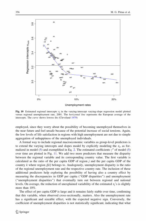
employed, since they worry about the possibility of becoming unemployed themselves in
the near future and feel unsafe because of the potential increase of social tensions. Again,
the low levels of life satisfaction in regions with high unemployment are not due to simple
aggregation of unhappiness of the unemployed individuals.
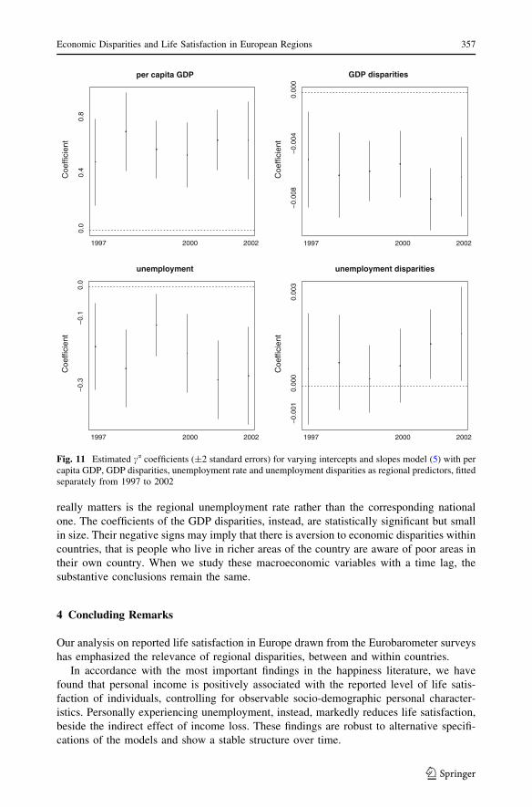
A formal way to include regional macroeconomic variables as group-level predictors is
to extend the varying intercepts and slopes model by explicitly modeling the aj, as for-
malized in model (5) and exemplified in Eq. 2. The estimated coefficients ca of model (5)
over time are plotted in Fig. 11. We add two more predictors that measure the disparity
between the regional variable and its corresponding country value. The first variable is
calculated as the ratio of the per capita GDP of region j and the per capita GDP of the
country k where region j[k] belongs to. Analogously, unemployment disparity is the ratio
of the regional unemployment rate and the respective country rate. The inclusion of these
additional predictors help exploring the possibility of having also a country effect by
measuring the discrepancies in GDP per capita (‘‘GDP disparities’’) and unemployment
(‘‘unemployment disparities’’) that eventually turn out between regional and national
levels. On average, the reduction of unexplained variability of the estimated aj’s is slightly
more than 10%.
The effect of per capita GDP is large and it remains fairly stable over time, confirming
that this variable, when observed cross-sectionally, matters. Also the unemployment rate
has a significant and sizeable effect, with the expected negative sign. Conversely, the
coefficient of unemployment disparities is not statistically significant, indicating that what
3.0
3.2
3.4
3.6
3.8
Unemployment rates
Reg
ress
ion
inte
rcep
ts α
nuts
0% 10% 20%
be1
be2
be3
dk
de1
de2
de3
de4
de5
de6
de7
de8de9
dea
deb
dec
ded
dee
def
deg
ie
gr1gr2
gr3
gr4
es1
es2
es3
es4
es5es6
es7
fr1fr2
fr3fr4
fr5fr6
fr7
fr8itc
itd
ite
itf itg
nl1
nl2nl3nl4
at1
at2at3
pt1
pt2pt3
fi
se
ukcukduke
ukf
ukg
ukh
uki
ukj
ukk
ukl
ukm
uknlu
Fig. 10 Estimated regional intercepts aj in the varying-intercept varying-slope regression model plottedversus regional unemployment rate, 2001. The horizontal line represents the European average of theintercepts. The curve shows lowess fits (Cleveland 1979)
356 M. G. Pittau et al.
123
really matters is the regional unemployment rate rather than the corresponding national
one. The coefficients of the GDP disparities, instead, are statistically significant but small
in size. Their negative signs may imply that there is aversion to economic disparities within
countries, that is people who live in richer areas of the country are aware of poor areas in
their own country. When we study these macroeconomic variables with a time lag, the
substantive conclusions remain the same.
4 Concluding Remarks
Our analysis on reported life satisfaction in Europe drawn from the Eurobarometer surveys
has emphasized the relevance of regional disparities, between and within countries.
In accordance with the most important findings in the happiness literature, we have
found that personal income is positively associated with the reported level of life satis-
faction of individuals, controlling for observable socio-demographic personal character-
istics. Personally experiencing unemployment, instead, markedly reduces life satisfaction,
beside the indirect effect of income loss. These findings are robust to alternative specifi-
cations of the models and show a stable structure over time.
per capita GDPC
oeffi
cien
t
1997 2000 2002
0.0
0.4
0.8
GDP disparities
Coe
ffici
ent
1997 2000 2002
−0.
008
−0.
004
0.00
0
unemployment
Coe
ffici
ent
1997 2000 2002
−0.
3−
0.1
0.0
unemployment disparitiesC
oeffi
cien
t
1997 2000 2002
−0.
001
0.00
00.
003
Fig. 11 Estimated ca coefficients (±2 standard errors) for varying intercepts and slopes model (5) with percapita GDP, GDP disparities, unemployment rate and unemployment disparities as regional predictors, fittedseparately from 1997 to 2002
Economic Disparities and Life Satisfaction in European Regions 357
123
Our main findings are that personal income matters, generally, more in poor regions
than in rich regions and this pattern still holds for regions within the same country. This
evidence is in line with the theory of Post-materialism, being life satisfaction in rich
societies more related to non-materialistic issues. From this perspective, it makes sense that
life satisfaction is more about economics in poor regions and more about ‘‘culture’’ in rich
regions. And it also makes sense that, among low-income individuals, reported level of
well-being are not much different in rich and poor societies, whereas the cultural differ-
ences between rich and poor societies become larger for the upper-middle class.
We also have found no evidence that dissatisfaction of being unemployed is lower in
regions where jobs are scarse and the opportunities of being re-employed are less. This
evidence does not support the hypothesis that individual unhappiness of being out of work
is influenced by local social standards (Warr and Jackson 1987), that is personal impact of
unemployment is alleviated in areas where unemployment is a typical condition.
Even after controlling for individual characteristics and different effects of income and
employment status across regions, we have found that the unexplained regional-level
variability of the estimated life satisfaction is still high, indicating that geography still
matters considerably.
The introduction in the model of regional per capita GDP and unemployment rate reduces
this variability by around 10% steadily over time and their effects are large and stable. This
evidence shows that these macroeconomic variables may help explaining differences in
reported subjective well-being across regions, but also other factors may be equally or more
influent. Since we have controlled for the personal level of income and employment status
and possible interactions, the effects of per capita GDP and unemployment rate go beyond
the simple aggregation of individual incomes and individual unemployment status. Unem-
ployment reduces life satisfaction also in individuals who are not out of work. This may be
due to the perception of an increasing risk of loosing a job or of being trapped in the job one
has, but also to aversion to social inequality. Regional per capita GDP, at least cross-
sectionally, also matters. Per capita GDP is positively correlated with several others factors
that could affect life satisfaction. It is well documented that in Europe GDP per capita is
highly correlated with levels and quality of basic facilities and services, such as transpor-
tation and communications systems, and with levels and quality of public institutions like
schools and hospitals, as well as with low levels of crime and corruption (Tanzi and Davoodi
2000). These factors might explain the size of the effect of regional GDP on happiness.
To account for country effects, we have also included indicators of disparity between
the regional and the corresponding national per capita GDP and unemployment rate. It
turns out that the effects of these macroeconomic regional variables largely sweep off the
effects that the corresponding country variables have on reported life satisfaction. Factors
affecting the subjective well-being are essentially local. An interesting progression of this
research would be to further disaggregate the territorial units, moving from the first level of
NUTS to the second or third level, also including the new EU members.
The technique of multilevel models has given us a natural framework for understanding
these patterns and for modeling hierarchical data, individual characteristics within Euro-
pean regions. With respect to traditional alternatives, multilevel modeling has allowed us
to estimate differences between large number of groups (in terms of variation between
groups) and to analyze data coming from different sources inside the same model.
Acknowledgments The authors thank the Columbia University, Applied Statistics Center, and theNational Science Foundation and National Institutes of Health for financial support. They also acknowledgeSapienza, University of Rome, for financial assistance under grant number C26F07R754. They would like to
358 M. G. Pittau et al.
123
thank an anonymous reviewer and participants of the XXX IARIW conference, Portoroz, Slovenia, August2008, for their precious comments and suggestions.
Appendix
See Table 1.
Table 1 Life satisfaction (LS) in European Regions (NUTS1), average 1992–2002
Country Region (NUTS1) Label LS Decile ranking
Belgium Region de Bruxelles be1 2.95 6
Belgium Vlaams Gewest be2 3.16 3
Belgium Region Wallonne be3 2.90 7
Denmark Denmark dk 3.61 1
Germany Baden-Wurttemberg de1 2.99 5
Germany Bayern de2 3.04 4
Germany Berlin de3 2.79 9
Germany Brandenburg de4 2.74 9
Germany Bremen de5 2.99 5
Germany Hamburg de6 2.88 7
Germany Hessen de7 3.01 5
Germany Mecklenburg-Vorpommern de8 2.73 9
Germany Niedersachsen de9 2.99 5
Germany Nordrhein-Westfalen dea 3.03 4
Germany Rheinland-Pfalz deb 2.97 6
Germany Saarland dec 3.02 5
Germany Sachsen ded 2.80 8
Germany Sachsen-Anhalt dee 2.75 9
Germany Schleswig-Holstein def 3.13 3
Germany Thuringen deg 2.73 10
Ireland Ireland ie 3.23 2
Greece Voreia Ellada gr1 2.65 10
Greece Kentriki Ellada gr2 2.58 10
Greece Attiki gr3 2.52 10
Greece Nisia Aigaiou, Kriti gr4 2.64 10
Spain Noroeste es1 2.94 6
Spain Noreste es2 3.02 5
Spain Comunidad de Madrid es3 2.86 8
Spain Centro (ES) es4 2.98 5
Spain Este es5 2.91 6
Spain Sur es6 2.88 7
Spain Canarias (ES) es7 2.90 7
France Ile de France fr1 2.85 8
France Bassin Parisien fr2 2.81 8
France Nord - Pas-de-Calais fr3 2.82 8
France Est fr4 2.87 7
Economic Disparities and Life Satisfaction in European Regions 359
123
References
Alesina, A., Di Tella, R., & MacCulloch, R. (2004). Inequality and happiness: Are Europeans and Amer-icans different. Journal of Public Economics, 88, 2009–2042.
Aslam, A., & Corrado, L. (2007). No man is an island: The inter-personal determinants of regional well-being and life satisfaction in Europe. Cambridge Working Paper in Economics, CWPE 0717.
Bertrand, M., & Mullainathan, S. (2001). Do people mean what they say? Implications for subjective surveydata. American Economic Review, 91, 67–72.
Table 1 continued
Country Region (NUTS1) Label LS Decile ranking
France Ouest fr5 2.91 6
France Sud-Ouest fr6 2.88 7
France Centre-Est fr7 2.87 7
France Mediterranee fr8 2.78 9
Italy Nord Ovest itc 2.93 6
Italy Nord Est itd 2.96 6
Italy Centro ite 2.86 8
Italy Sud itf 2.78 9
Italy Isole itg 2.73 9
Netherland Noord-Nederland nl1 3.36 1
Netherland Oost-Nederland nl2 3.41 1
Netherland West-Nederland nl3 3.37 1
Netherland Zuid-Nederland nl4 3.37 1
Austria Ostosterreich at1 3.10 4
Austria Sudosterreich at2 3.18 2
Austria Westosterreich at3 3.19 2
Portugal Continente pt1 2.63 10
Portugal Regiao Autonoma dos Acores pt2 2.85 8
Portugal Regiao Autonoma da Madeira pt3 2.77 8
Finland Finland fi 3.14 3
Sweden Sweden se 3.34 1
UK North East ukc 3.15 3
UK North West ukd 3.09 4
UK Yorkshire and The Humber uke 3.14 3
UK East Midlands ukf 3.19 2
UK West Midlands ukg 3.09 4
UK Eastern ukh 3.20 2
UK London uki 3.10 4
UK South East ukj 3.19 2
UK South West ukk 3.17 3
UK Wales ukl 3.16 3
UK Scotland ukm 3.07 4
UK Northern Ireland ukn 3.25 2
Luxembourg Luxembourg (Grand-Duche) lu 3.32 1
Source: Authors’ calculations on Mannheim Eurobarometer trend file
360 M. G. Pittau et al.
123
Blanchflower, D. G., & Oswald, A. J. (2004). Well-being over time in Britain and the USA. Journal ofPublic Economics, 88, 1359–1386.
Clark, A. (2003). Unemployment as a social norm: Psychological evidence from panel data. Journal ofLabor Economic, 21(2), 323–351.
Clark, A., & Oswald, A. J. (1994). Unhappiness and unemployment. Economic Journal, 104, 648–659.Cleveland, W. S. (1979). Robust locally weighted regression and smoothing scatter plots. Journal of
American Statistical Association, 74, 829–836.Diener, E. Sandvik, E., Seidlitz, L., & Diener, M. (1993). The relationship between income and subjective
well-being: Relative or absolute? Social Indicators Research, 28, 195– 223.Di Tella, R., MacCulloch, R., & Oswald, A. J. (2001). Preferences over inflation and unemployment:
Evidence from happiness surveys. American Economic Review, 91(1), 335–42.Di Tella, R., MacCulloch, R., & Oswald, A. J. (2003). The macroeconomics of happiness. Review of
Economics and Statistics, 85, 809–827.Easterlin, R. A. (1974). Does economic growth improve the human lot? Some empirical evidence. In P.
David & M. Reder (Eds.), Nations and households in economic growth. New York: Academic Press.European Commission. (2008). A new partnership for cohesion convergence competitiveness cooperation.
Third report on economic and social cohesion.Ferrer-i-Carbonell, A., & Frijters, P. (2004). How important is methodology for the estimates of the
determinants of happiness? Economic Journal, 114, 641–659.Frey, B. S., & Stutzer, A. (2000). Happiness, economy and institutions. Economic Journal, 110, 918–938.Frey, B. S., & Stutzer, A. (2002). Happiness and economics: How the economy and institutions affect human
well-being. Princeton: Princeton University Press.Frey, B. S., & Stutzer, A. (2006). Does marriage make people happy, or do happy people get married.
Journal of Socio-Economics, 35(2), 326–347.Gelman, A., & Hill, J. (2007). Data analysis using regression and multilevel/hierarchical models. Cam-
bridge: Cambridge University Press.Gelman, A., Park, D. K., Shor, B., Bafumi J., & Cortina G. (2008b). Red state, blue state, rich state, poor
state: Why Americans vote the way they do. Princeton: Princeton University Press.Gelman, A., Shor, B., Bafumi, J., & Park, D. (2008a). Rich state, poor state, red state, blue state: What’s the
matter with Connecticut? Quarterly Journal of Political Science, 2, 345–367.Graham, C., & Felton, A. (2006). Inequality and happiness: Insights from Latin America. Journal of
Economic Inequality, 4(1), 1569–1721.Inglehart, R. (1990). Culture shift in advanced industrial society. Princeton: Princeton University Press.Kahneman, D., & Krueger, A. B. (2006). Developments in the measurement of subjective well-being.
Journal of Economic Perspectives, 20(1), 3–24.Krueger, A. B., & Schkade, D. A. (2007). The reliability of subjective well-being measures. NBER Workin
Paper No. 13027.Layard, R. (2005). Happiness: Lessons from a new science. New York: Penguin Press.Longford, N. T. (2007). Missing data and small-area estimation. New York, NY: Springer-Verlag.Oswald, A. J.(1997). Happiness and economic performance. Economic Journal, 107, 1815– 1831.Pittau, M. G., & Zelli, R. (2006). Empirical evidence of income dynamics across EU regions. Journal of
Applied Econometrics, 21, 605–628.R Development Core Team. (2006). R: A language and environment for statistical computing. Vienna,
Austria: R Foundation for Statistical Computing.Schmitt, H., & Scholz, E. (2005). The Mannheim Eurobarometer Trend File, 1970–2002 [Computer file].
Prepared by Zentralarchiv fur Empirische Sozialforschung. ICPSR04357-v1. Mannheim, Germany:Mannheimer Zentrum fur Europaische Sozialforschung and Zentrum fur Umfragen, Methoden undAnalysen [producers]. Cologne, Germany: Zentralarchiv fur Empirische Sozialforschung/Ann Arbor,MI: Inter-university Consortium for Political and Social Research [distributors].
Scoppa, V., & Ponzo, M. (2008). An empirical study of happiness in Italy. B. E. Journal of EconomicAnalysis and Policy, 8(1) (Contributions), article 15.
Snijders, T. A. B., & Bosker, R. J. (1999). Multilevel analysis. London: Sage.Tanzi, V., & Davoodi, H. R. (2000). Corruption, growth and public finances. IMF Working Paper No. 182.Veenhoven, R. (2007). World database of happiness, distributional findings in nations. Rotterdam: Erasmus
University.Warr, P. B., & Jackson, P. (1987). Adopting to the unemployed role; a longitudal investigation. Social
Science Medicine, 25, 1219–1224.Wilkinson, W. (2007). In pursuit of happiness research. Is it reliable? What does it imply for policy? Policy
Analysis, 590, 1–41.Winkelmann, L., & Winkelmann, R. (1998). Why are the unemployed so unhappy? Economica, 65(257), 1–15.
Economic Disparities and Life Satisfaction in European Regions 361
123