1

Economic convergence and the fundamental equilibrium

exchange rate in Poland1

Michał Rubaszek*)

Abstract:

The paper presents an extended version of the fundamental equilibrium exchange rate model

(FFER). By introducing potential output into the specification of the foreign trade equations

of the partial equilibrium FEER model we show that, under some plausible assumptions, the

calculated level of the equilibrium exchange rate is consistent with the estimates of the

behavioral equilibrium exchange (BEER). Moreover, we indicate that including the terms of

trade as an explanatory variable in a reduced-form BEER equation for the real exchange rate

might lead to the indeterminacy of the parameter estimates. The proposed model is applied to

analyze fluctuations of the Polish zloty. We show that the real appreciation of the zloty is to a

largely an equilibrium phenomenon.

JEL classification: C32, F12, F31

Keywords: Fundamental equilibrium exchange rate, current account, foreign trade.

*) Economic Institute National Bank of Poland michal.rubaszek@mail.nbp.pl

First draft, 29 September 2008

Not for citation nor distribution

1 The author thanks Łukasz Rawdanowicz for very useful comments.

2

1. Introduction

The growing literature on equilibrium exchange rates (EER) of central and eastern European

countries (CEECs), reviewed e.g. by Égert (2003), has predominantly applied two concepts:

behavioral EER and fundamental EER. The BEER, proposed by Clark and MacDonald

(1998), is mostly empirical in nature and in most cases not explicitly supported by theoretical

considerations. The BEER can be shortly characterized as the theoretical value of an

estimated single-equation, cointegration model for the real exchange rate (RER). Among the

medium-term determinants of the RER, relative productivity, net foreign assets and the terms

of trade are the most frequently used in the empirical applications. The FEER, presented by

Williamson (1994), uses a complete macroeconomic model of an economy, or a partial

equilibrium model of foreign trade, to find the level of the RER that would be consistent with

the simultaneous attainment of internal and external equilibrium. In most studies internal

equilibrium is defined as null output gap and external equilibrium as the current account equal

to its exogenously set target.

The two EER approaches to modeling CEECs’ exchange rates tend to be considered

complementary rather that substituting. This might be due to the fact that in the standard

specification of the FEER model an increase in domestic output leads to a deterioration in the

current account, which requires a depreciation of domestic currency. This was shown by

Clark and MacDonald (1998), who solved the FEER model to derive a reduced-form single

equation for the RER in which an increase in domestic output is weakening the domestic

currency. This is, however, contradicting the empirical findings pointing to a significant and

positive relationship between the GDP per capita and the real exchange rate (see. e.g. Balassa,

1964).

The problem with the application of the FEER concept to transition economies was discussed

by Maeso-Fernandez et al. (2005). The authors claim that changes in productivity are not

accounted for in this approach, whereas the catching-up process is one of the central

arguments of the equilibrium exchange rate appreciation in CEECs. In other words, the

standard specification of trade equations in the FEER model does not take into account that

real exchange rate appreciation related to the process of real convergence should not have

negative effects on the current account balance. Two studies tried to address this issue. Égert

3

and Lahrèche-Révil (2003) proposed a tree-equation vector autoregression model that

combines a relationship between relative productivity and the real exchange rate, which is

empirically supported by the BEER literature, with external equilibrium concept of the FEER.

In the second study, Bulíř and Šmídková (2005) extended the specification of trade equations

of the traditional FEER model by including the inward stock of foreign direct investment

(FDI). Their model implies that inflows of FDI were the main reason behind the process of

real exchange rate appreciation in CEECs.

In this paper we address the above-mentioned discrepancy between the BEER and FEER

concepts by introducing potential output into the specification of the foreign trade equations.

We show that the BEER equation is, under some plausible assumptions, a reduced form of our

FEER model. Moreover, we indicate that if our specification is correct, including the terms of

trade as an explanatory variable in a reduced-form BEER equation for the real exchange rate

might lead to the indeterminacy of the parameter estimates. The proposed model is applied to

analyze fluctuations of the Polish zloty.

The structure of the article is as follows. Section 2 discusses issues concerning the

specification of trade equations in converging economies. Section 3 describes the FEER

model. In Section 4 we present the results of FEER estimates for the Polish zloty. Section 5

investigates the sensitivity of equilibrium exchange rate with respect to the normative

assumptions of the FEER model. In section 6 we derive the reduced-form equation for the real

exchange rate. The last section summarizes the main findings of the paper and concludes.

2. Foreign trade and economic transformation in Poland

Foreign trade equations are the heart of the partial equilibrium FEER model. In most

applications of the FEER (e.g. Williamson, 1994, for the G7 economies and Coudert and

Couharde, 2003, for CEECs) the specification of the foreign trade equations is of Armington’s

(1969) type, which assumes that each country produces one variety or the consumer perceives

varieties originating from a country as perfect substitutes. This implies that export demand is

determined solely by two factors: foreign demand and relative prices. In this model, an

increase in the share in foreign markets involves deterioration in the terms of trade and thus

real exchange rate depreciation, which is clearly in opposition to the Polish experience. While

in the period 1995-2007 the share of Poland in world imports more than doubled, the GDP

4

deflator based real effective exchange rate of the Polish zloty appreciated by about 50% (see

Figure 1).

Figure 1. The share in world imports and RERs of Poland

80

100

120

140

160

1995

1996

1997

1998

1999

2000

2001

2002

2003

2004

2005

2006

2007

2008

199

5:1=

100

50

100

150

200

250

199

5:1=

100

Real effective exchange rate (LHS) Share in world imports (RHS)

Source: IMF Directions of Trade Statistics, Eurostat, OECD Main Economic Indicators.

The rapid growth of Poland’s share in the world trade since the beginning of the

transformation was rather due to supply factors, namely profound changes in the sectoral

composition of output and ownership structure of firms. These changes, which are not

accounted for in the standard specification of the foreign trade equations, have had

tremendous effects on patterns of the foreign trade, both in terms of its geographical and

sectoral composition. Although the detailed analysis of the foreign trade changes in Poland is

not the focus of this paper, we point here to a few of the most important facts that have had

impact on Polish trade:

� substantial inflows of foreign direct investment enhanced intra-firm trade between

western European and Polish firms (Lane and Gian Maria Milesi-Ferretti, 2007);

� EU integration and reduction in impediments to trade resulted in a rapid growth of

intra-industry trade both in horizontally and vertically differentiated goods, which

has been reflected, among others, by the increasing share of trade in intermediate

goods in total trade;

� gradual change in the export structure from labor-intensive products, for instance

textiles, into more capital and skill intensive goods such as motor vehicles and

electrical machinery (see Table 1).

5

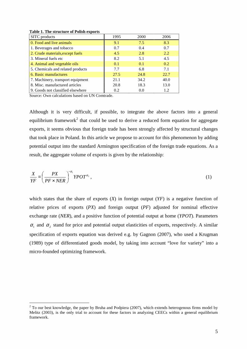
Table 1. The structure of Polish exports SITC products 1995 2000 2006

0. Food and live animals 9.1 7.5 8.3 1. Beverages and tobacco 0.7 0.4 0.7 2. Crude materials,except fuels 4.5 2.8 2.2 3. Mineral fuels etc 8.2 5.1 4.5 4. Animal and vegetable oils 0.1 0.1 0.2 5. Chemicals and related products 7.7 6.8 7.1 6. Basic manufactures 27.5 24.8 22.7 7. Machinery, transport equipment 21.1 34.2 40.0 8. Misc. manufactured articles 20.8 18.3 13.0 9. Goods not classified elsewhere 0.2 0.0 1.2

Source: Own calculations based on UN Comtrade.

Although it is very difficult, if possible, to integrate the above factors into a general

equilibrium framework2 that could be used to derive a reduced form equation for aggregate

exports, it seems obvious that foreign trade has been strongly affected by structural changes

that took place in Poland. In this article we propose to account for this phenomenon by adding

potential output into the standard Armington specification of the foreign trade equations. As a

result, the aggregate volume of exports is given by the relationship:

2

1

αα

YPOTNERPF

PX

YF

X−

×= , (1)

which states that the share of exports (X) in foreign output (YF) is a negative function of

relative prices of exports (PX) and foreign output (PF) adjusted for nominal effective

exchange rate (NER), and a positive function of potential output at home (YPOT). Parameters

1α and 2α stand for price and potential output elasticities of exports, respectively. A similar

specification of exports equation was derived e.g. by Gagnon (2007), who used a Krugman

(1989) type of differentiated goods model, by taking into account “love for variety” into a

micro-founded optimizing framework.

2 To our best knowledge, the paper by Bruha and Podpiera (2007), which extends heterogenous firms model by Melitz (2003), is the only trial to account for these factors in analyzing CEECs within a general equilibrium framework.

6

3. The FEER model

The empirical application of the partial equilibrium FEER model consists of the three

following stages. First, the parameters of the foreign sector model of an economy are

estimated. The model is then simulated to find a relationship between the current account and

the real exchange rate. Finally, the FEER is computed as the level of the real exchange rate

that equalizes the model’s implied current account, assuming that output gaps at home and

abroad are closed, with its exogenously set target level. This implies that the calculations of

the FEER involve (i) estimating or calibrating the foreign trade equations, (ii) computing the

level of potential output at home and abroad, and (iii) setting the target for the current account

balance.

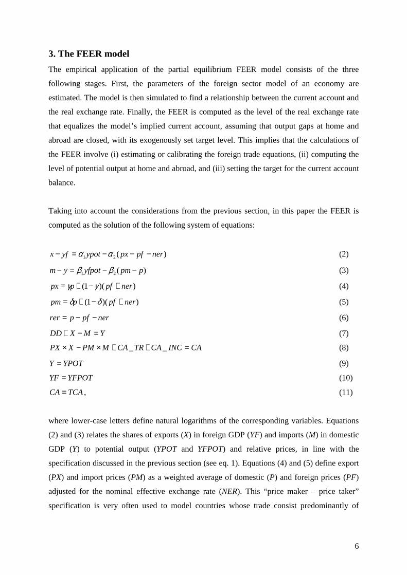
Taking into account the considerations from the previous section, in this paper the FEER is

computed as the solution of the following system of equations:

)(21 nerpfpxypotyfx −−−=− αα (2)

)(21 ppmyfpotym −−=− ββ (3)

))(1( nerpfppx +−+= γγ (4)

))(1( nerpfppm +−+= δδ (5)

nerpfprer −−= (6)

YMXDD =−+ (7)

CAINCCATRCAMPMXPX =++×−× __ (8)

YPOTY = (9)

YFPOTYF = (10)

TCACA = , (11)

where lower-case letters define natural logarithms of the corresponding variables. Equations

(2) and (3) relates the shares of exports (X) in foreign GDP (YF) and imports (M) in domestic

GDP (Y) to potential output (YPOT and YFPOT) and relative prices, in line with the

specification discussed in the previous section (see eq. 1). Equations (4) and (5) define export

(PX) and import prices (PM) as a weighted average of domestic (P) and foreign prices (PF)

adjusted for the nominal effective exchange rate (NER). This “price maker – price taker”

specification is very often used to model countries whose trade consist predominantly of

7

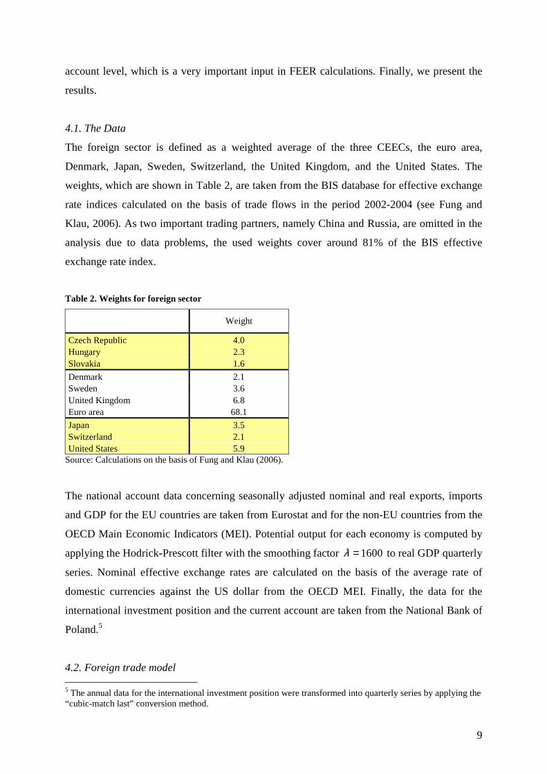
differentiated manufactured products. Given the definition of the real effective exchange rate

(eq. 6), exports and imports price competitiveness measures are equal to:

rernerpfpx γ=−− )( (12)

rerppm )1()( −=− δ (13)

Relationships (7) and (8) are GDP and current account identities, respectively: GDP is the

sum of domestic demand (DD) and net trade, whereas the current account is the sum of

balances on trade, current transfers (CA_TR) and income (CA_INC). Finally, equations (9)-

(11) express the internal and external balance conditions, stating that foreign and domestic

output gaps are closed and the current account balance is equal to its target level (TCA). Given

the exogenously set values of YPOT, YFPOT and TCA,3 the model can be solved for domestic

demand and the real exchange rate ensuring the simultaneous attainment of the internal and

external equilibria. The solution for the real exchange rate is called FEER.

The system given by equations (2)-(11) can be illustrated by a Swan diagram, as presented in

Figure 2. The horizontal axis represents domestic demand and the vertical axis represents the

real exchange rate, where an upward movement stands for domestic currency appreciation.

The internal equilibrium locus (IE) is sloped upward as a rise in domestic demand requires a

proportional decline in net trade, and thereby real exchange rate appreciation, so that the

output gap remained closed. As regards the external equilibrium locus (EE), it is sloped

downward as current account deterioration entailed by stronger domestic demand has to be

counterbalanced by domestic currency depreciation, so that the current account remained at its

target level. The intersection of the internal and external loci defines the FEER and the

corresponding, equilibrium level of domestic demand.

3 And other exogenous variables of the model such as PF, YF, P, CA_TR and CA_INC, which in opposition to Y_POT, YF_POT and TCA are observable.

8

Figure 2. Solution for the FEER

IE

EE

Domestic Demand

Exc

hang

e R

ate

DDFEER

FEER

Istrong demand

current account deficit

IIweak demand

current account deficit

IIIweak demand

current account surplus

IVstrong demand

current account surplus

Source: Adopted from Rosenberg (1996, p. 32)

The analysis of Figure 2 shows that within this framework there are four cases of economic

disequilibrium. The first (third) quadrant represents a country with excessive (subdued)

domestic demand, which leads to a current account deficit (surplus)4 and a positive (negative)

output gap. On the other hand, the second (fourth) quadrant is an example of a country with

an overvalued (undervalued) real exchange rate. The weak (strong) external price

competitiveness, in turn, results in a negative (positive) output gap and a current account

deficit (surplus). The policy implications are twofold. First, if a country is running a current

account deficit (surplus) and the output gap is negative (positive) then it is a clear signal that

the real exchange rate is overvalued (undervalued). Second, if domestic demand is excessive

(subdued) then setting the real exchange rate at its fundamental level does not guarantee that

the economy will return to its fundamental equilibrium. In most cases reaching the

fundamental equilibrium requires both: adjustment in the real exchange rate and domestic

demand.

4. Empirical evidence

In this section we illustrate how the FEER model can be empirically tested by applying the

concept to analyze the equilibrium value of the Polish zloty. We start by discussing the data

issues. Then, we move to estimates of the foreign trade model given by equations 2-3 and 12-

13. The next sub-section discusses the normative assumption concerning the target current

4 Here a current account deficit should be interpreted as a current account balance that is below the target current account.

9

account level, which is a very important input in FEER calculations. Finally, we present the

results.

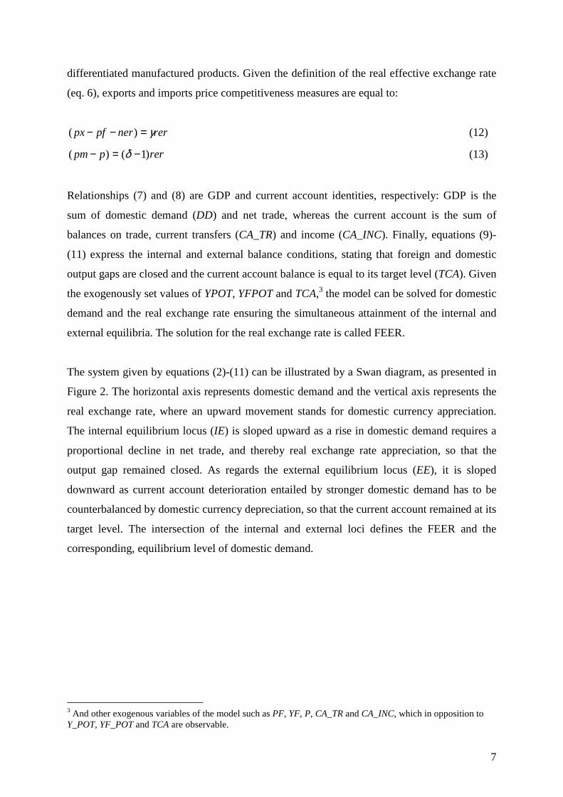
4.1. The Data

The foreign sector is defined as a weighted average of the three CEECs, the euro area,

Denmark, Japan, Sweden, Switzerland, the United Kingdom, and the United States. The

weights, which are shown in Table 2, are taken from the BIS database for effective exchange

rate indices calculated on the basis of trade flows in the period 2002-2004 (see Fung and

Klau, 2006). As two important trading partners, namely China and Russia, are omitted in the

analysis due to data problems, the used weights cover around 81% of the BIS effective

exchange rate index.

Table 2. Weights for foreign sector

Weight

Czech Republic 4.0 Hungary 2.3 Slovakia 1.6

Denmark 2.1 Sweden 3.6 United Kingdom 6.8 Euro area 68.1

Japan 3.5 Switzerland 2.1 United States 5.9

Source: Calculations on the basis of Fung and Klau (2006).

The national account data concerning seasonally adjusted nominal and real exports, imports

and GDP for the EU countries are taken from Eurostat and for the non-EU countries from the

OECD Main Economic Indicators (MEI). Potential output for each economy is computed by

applying the Hodrick-Prescott filter with the smoothing factor 1600=λ to real GDP quarterly

series. Nominal effective exchange rates are calculated on the basis of the average rate of

domestic currencies against the US dollar from the OECD MEI. Finally, the data for the

international investment position and the current account are taken from the National Bank of

Poland.5

4.2. Foreign trade model 5 The annual data for the international investment position were transformed into quarterly series by applying the “cubic-match last” conversion method.

10

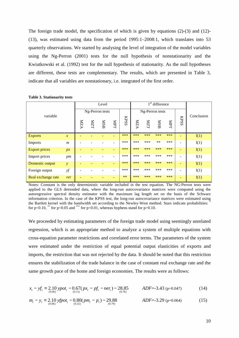
The foreign trade model, the specification of which is given by equations (2)-(3) and (12)-

(13), was estimated using data from the period 1995:1–2008:1, which translates into 53

quarterly observations. We started by analysing the level of integration of the model variables

using the Ng-Perron (2001) tests for the null hypothesis of nonstationarity and the

Kwiatkowski et al. (1992) test for the null hypothesis of stationarity. As the null hypotheses

are different, these tests are complementary. The results, which are presented in Table 3,

indicate that all variables are nonstationary, i.e. integrated of the first order.

Table 3. Stationarity tests

Level 1st difference

Ng-Perron tests Ng-Perron tests variable

MZ

A

MZ

T

MS

B

MP

T

KP

SS

MZ

A

MZ

T

MS

B

MP

T

KP

SS

Conclusion

Exports x - - - - *** *** *** *** *** - I(1)

Imports m - - - - *** *** *** ** *** - I(1)

Export prices px - - - - *** *** *** *** *** - I(1)

Import prices pm - - - - *** *** *** *** *** - I(1)

Domestic output y - - - - *** *** *** *** *** - I(1)

Foreign output yf - - - - *** *** *** *** *** - I(1)

Real exchange rate rer - - - - ** *** *** *** *** - I(1)

Notes: Constant is the only deterministic variable included in the test equation. The NG-Perron tests were applied to the GLS detrended data, where the long-run autocovariance matrices were computed using the autoregressive spectral density estimator with the maximum lag length set on the basis of the Schwarz information criterion. In the case of the KPSS test, the long-run autocovariance matrices were estimated using the Bartlett kernel with the bandwidth set according to the Newley-West method. Stars indicate probabilities: * for p<0.10, ** for p<0.05 and *** for p<0.01, whereas hyphens stand for p>0.10.

We proceeded by estimating parameters of the foreign trade model using seemingly unrelated

regression, which is an appropriate method to analyze a system of multiple equations with

cross-equation parameter restrictions and correlated error terms. The parameters of the system

were estimated under the restriction of equal potential output elasticities of exports and

imports, the restriction that was not rejected by the data. It should be noted that this restriction

ensures the stabilization of the trade balance in the case of constant real exchange rate and the

same growth pace of the home and foreign economies. The results were as follows:

)76.0()11.0()06.0(85.28)(67.010.2 −−−−=− tttttt nerpfpxypotyfx ADF=-3.43 (p=0.047) (14)

)79.0()21.0()06.0(88.29)(80.010.2 −−−=− ttttt ppmyfpotym ADF=-3.29 (p=0.064) (15)

11

)06.0()07.0(17.074.0 −=−− tttt rernerpfpx ADF=-7.06 (p=0.000) (16)

)05.0()06.0(13.016.0 −−=− ttt rerppm , ADF=-4.48 (p=0.000) (17)

where the figures in parentheses stand for the standard deviation of estimates. All estimates

are of correct sign and acceptable magnitude. The price elasticity of exports and imports,

amounting to 0.67 and 0.80 respectively, is moderate and comparable to the findings of the

literature (e.g. Faruqee and Isard, 1998). In the case of the potential output elasticity, the

estimate of 2.10 is high and significant, supporting our hypothesis that trade flows are to a

large extent driven by supply factors. As for the price equations, the results indicate that

Poland is predominantly a price-maker country, which is rather in opposition to our prior

expectations. Finally, it should be noticed that according to the ADF test, the residuals of all

relationships are stationary at 10% significance level and thereby these relationships might be

classified as cointegrating ones.6

4.3. Target current account

A large part of international capital flows might be classified as short-term and speculative.

These kinds of flows are influenced by the relative monetary policy stance, expectations

concerning temporary nominal exchange rate trends or changes in risk premium. Moreover, in

the short term, capital flows might also be affected by a one-off adjustment in the portfolio

structure of financial institutions or large FDI, the effects of which vanish in the medium run.

In the article, we define the “target current account” as a value of the current account that

abstracts from the above short-term capital flows.

In the literature there are several methods for calculating the medium-term current account

balance. Below, we refer to the two most frequently used in the empirical studies on Poland

and other CEECs. The first one, the theoretical foundations of which are based on the

intertemporal approach to the current account, considers the medium-term capital flows as a

reflection of life-time decisions of economic agents concerning savings and investment. The

empirical application involves the estimation of a reduced-form panel equation relating the

current account to a set of standard macroeconomic fundamentals, such as relative GDP per

capita, the demographic structure and fiscal policy. The most prominent examples of this

analytical approach are the studies by Debelle and Faruquee (1996) or Chinn and Prasad 6 The p-values are calculated using MacKinnon (1996) programs for cointegration tests.

12

(2003). As regards the results of this kind of estimates for Poland, Doisy and Herve (2003)

found that the target level for the current account deficit in 1999 ranged from 3.1% to 4.9% of

GDP, Bussière et al. (2004) indicated that in 2002 Poland would run a current account deficit

in the range from 2.4% to 5.2% of GDP, whereas Abiad et al. (2006) estimated that in the

years 1997-2004 the current account deficit in Poland should have fluctuated between 6% and

10% of GDP.

The second approach, proposed by Milesi-Ferretti and Razin (1996), treats the current account

as an increment to the stock of net foreign assets. The current account is considered to be

sustainable if it does not endanger the intertemporal solvency of the country, or in other

words, does not lead to an excessive build-up of foreign liabilities. As regards the relevant

studies for Poland, Zanghieri (2004) calculated that the sustainable current account deficit

ranges from 4.3% to 8.3% of GDP, whereas Aristovnik (2006) indicated a range between

1.0% and 5.0% of GDP. The differences in the results can be explained by different

assumptions concerning net FDI inflows, potential growth rate or the steady-state level of

external debt.

In this article we calculate the level of the target current account using an extended version of

the Milesi-Ferretti and Razin framework, which incorporates the convergence of net foreign

assets to a steady-state level and valuation effects. We start by describing the law of motion

for the stock of net foreign assets (Bt):

tttt VECABB ++= −1 , (18)

where VEt stands for valuation effects. Dividing the above equation by nominal GDP leads to

the following specification:

tttttt vecapybb ++∆−∆−= − )1(1 (19)

13

where the lower-case letters define the ratios with respect to GDP. Given the convergence of

net foreign assets to a steady-state level (b ):

)( 1 bbb tt −−=∆ −ρ , (20)

the target level of the current account can be calculated as:

tttttt veypbbbtca −∆+∆+−= −− )()( 11ρ . (21)

According to the above expression, in the medium term the current account might differ from

zero for the three following reasons: (i) to allow the adjustment of net foreign assets to a

steady-state, (ii) positive growth of nominal GDP and (iii) the existence of valuation effects.

In the empirical application, the parameterization of equation (21) is as follows. The

convergence path ρ is set to 0.025 so that within a quarter there is a fall of 2.5% in the

distance between the actual and steady-state level of net foreign assets. Following Bulíř and

Šmídková (2005) the steady-state level of net foreign liabilities b is chosen to be 65% of

annual GDP. As regards the growth rates of prices p∆ and output y∆ , we take the inflation

target of 2.5% per year and potential output growth. Finally, we assume that valuation effects

are equal to some fraction of net foreign assets:

1−= tt bve κ , (22)

where we set 01.0=κ to reflect the 2000-2006 historical average for the case of Poland.

The results of calculated current account deficit are presented in Table 4. They show that

between 2000 and 2004 the target current deficit improved gradually from 4.0% to 3.5% of

GDP, which was associated with a deterioration in the international investment position.

14

Thereafter, it increased slightly, amounting to 3.8% of GDP in 2008:1 due to an acceleration

in potential output growth. It should be noted, that our results are broadly in line with the

findings of the studies reviewed above.

Table 4. Target current account calculations

Data (annual average) Target current account decomposition

tb

(% of GDP) tp∆

(%, QoQ) ty∆

(%, QoQ) ttca )( 1 bbt −−ρ

convergence

)(1 ttt ypb ∆+∆−

output growth tve−

val. effects 2000 -122 0.6 0.8 -4.0 -3.5 -1.8 1.2 2001 -117 0.6 0.8 -4.0 -3.5 -1.6 1.2 2002 -125 0.6 0.8 -4.0 -3.5 -1.7 1.2 2003 -153 0.6 0.9 -3.6 -2.8 -2.2 1.5 2004 -162 0.6 1.0 -3.5 -2.4 -2.7 1.6 2005 -162 0.6 1.2 -3.7 -2.5 -2.9 1.6 2006 -170 0.6 1.3 -3.8 -2.3 -3.2 1.7 2007 -175 0.6 1.3 -3.8 -2.1 -3.4 1.7

08q1 -177 0.6 1.3 -3.8 -2.1 -3.4 1.8

4.4. Estimates of the FEER

We start the estimation of the FEER by calculating an underlying current account, i.e. the

current account that would prevail if:

� domestic and foreign output gaps were null;

� trade volumes and prices were at their medium-term levels;

� the transfer and income balances were adjusted for temporary factors.

In this regard, we calculate the underlying trade balance by taking the theoretical values for

export and import prices and volumes from equations (14)-(17), given that internal balance

conditions (9) and (10) are met. The adjustment of income and transfer balances for

temporary factors is done by using the Hodrick-Prescott filter. The underlying current account

is subsequently calculated according to definition given by equation (8). The results, as

presented in Figure 3, show that for most of the period 2000:1-2008:1 the underlying current

account fluctuated at levels above the target current account, where the difference was the

most evident at the turn of 2004. The only exceptions are the years 2001-2002 and the first

quarter of 2008, when the underlying current account stood below its target level. Within the

FEER framework, a high (low) level of the underlying current account balance means that the

real exchange rate is undervalued (overvalued), where the scale of real exchange rate

misalignment is positively related to the difference between the underlying and target current

account.

15

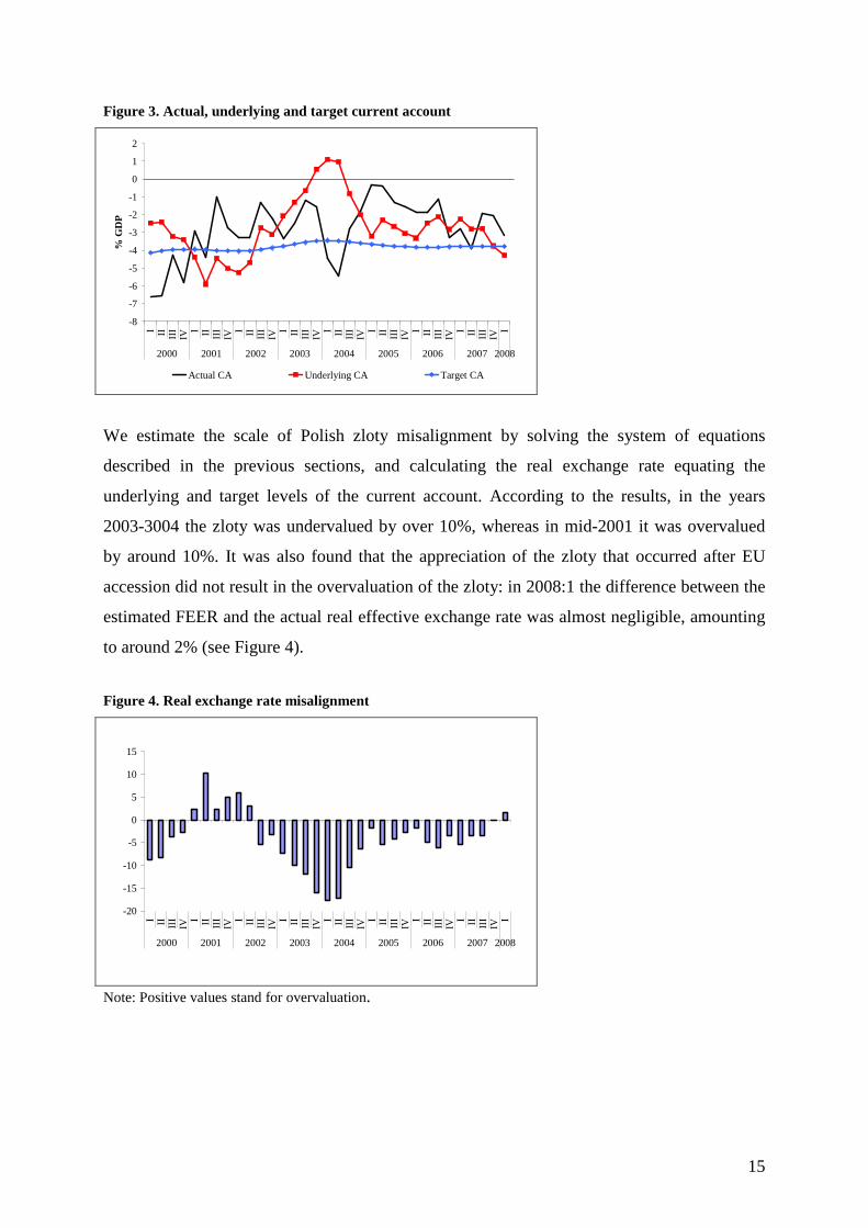
Figure 3. Actual, underlying and target current account

-8

-7

-6

-5

-4

-3

-2

-1

0

1

2I II III IVI II III IVI II III IVI II III IVI II III IVI II III IVI II III IVI II III IVI

2000 2001 2002 2003 2004 2005 2006 2007 2008

% G

DP

Actual CA Underlying CA Target CA

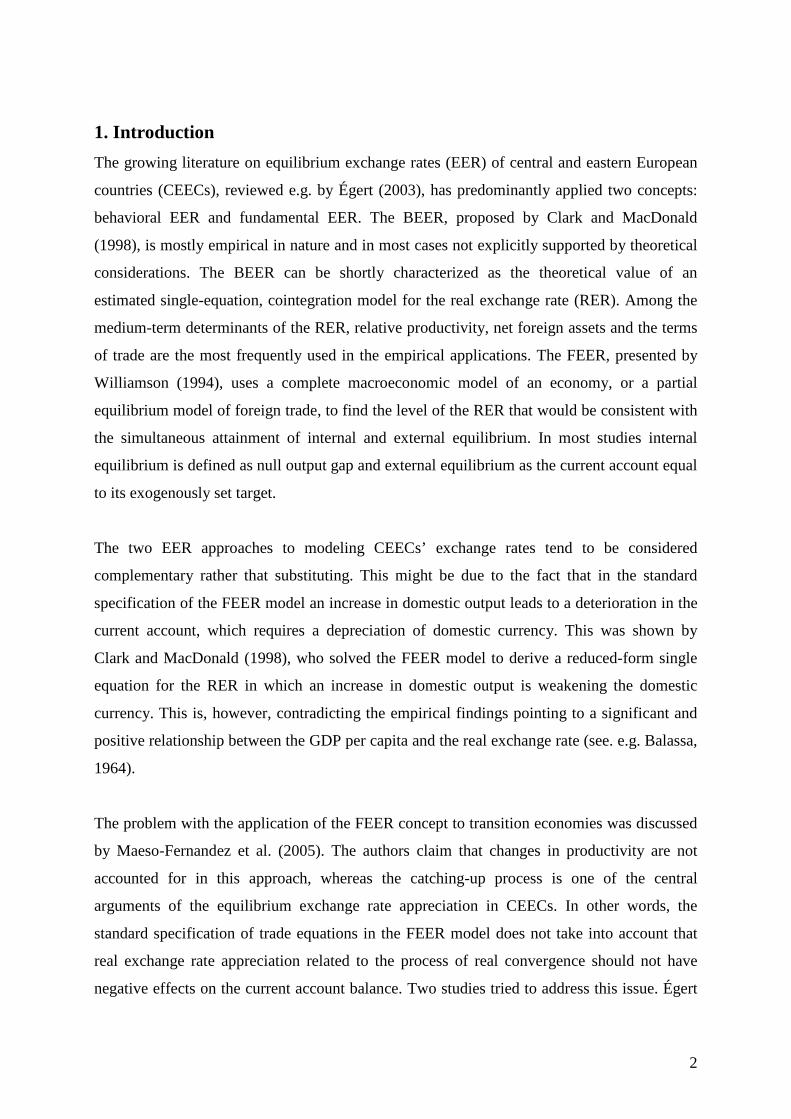
We estimate the scale of Polish zloty misalignment by solving the system of equations

described in the previous sections, and calculating the real exchange rate equating the

underlying and target levels of the current account. According to the results, in the years

2003-3004 the zloty was undervalued by over 10%, whereas in mid-2001 it was overvalued

by around 10%. It was also found that the appreciation of the zloty that occurred after EU

accession did not result in the overvaluation of the zloty: in 2008:1 the difference between the

estimated FEER and the actual real effective exchange rate was almost negligible, amounting

to around 2% (see Figure 4).

Figure 4. Real exchange rate misalignment

-20

-15

-10

-5

0

5

10

15

I II III IVI II III IVI II III IVI II III IVI II III IVI II III IVI II III IVI II III IVI

2000 2001 2002 2003 2004 2005 2006 2007 2008

Note: Positive values stand for overvaluation.

16

5. Sensitivity analysis

The FEER estimates are as plausible as the underlying foreign trade model and the

assumptions for potential output and the target current account. These assumptions, however,

are based on some normative judgment and calculations and thereby surrounded by a high

degree of uncertainty. For that reason, the application of the FEER method in estimating real

exchange rate misalignments might be considered incomplete, if it is not accompanied by a

sensitivity analysis. As stated by Driver and Wren-Lewis (1999), the assessment of the FEER

estimates with respect to the model’s assumptions might address two sets of issues: (i) those

related to the parameterization and specification of the foreign trade model, and (ii) those

related to the exogenous variables of the FEER model. In this paper we focus on the second

aspect of the sensitivity analysis, i.e. we answer the question: how FEER estimates are

affected by the changes in the assumed levels of potential output and the target current

account. We do it using both, graphs and analytical calculations.

As regards the relationship between the assumed level of potential output and the FEER, it is

illustrated in the left-hand panel of Figure 4. Higher potential output at home is shifting the

internal balance curve IE to the right, as growth in aggregate supply requires an increase in

aggregate demand of the same magnitude, so that internal equilibrium condition is satisfied.

Moreover, if the potential output elasticity of exports 1α is above unity, growth in the supply-

side performance of the economy is also improving the underlying current account, and thus

shifts the external balance curve EE to the right. The result for the real exchange rate is

appreciation, where the analytical proof of this result is presented in the further part of this

section. The effects of changes in the assumed level of the target current account are

illustrated in the right-hand panel of Figure 5. A higher target current account balance means

a leftward shift of the external equilibrium curve, and thereby requires lower domestic

demand and weaker domestic currency.

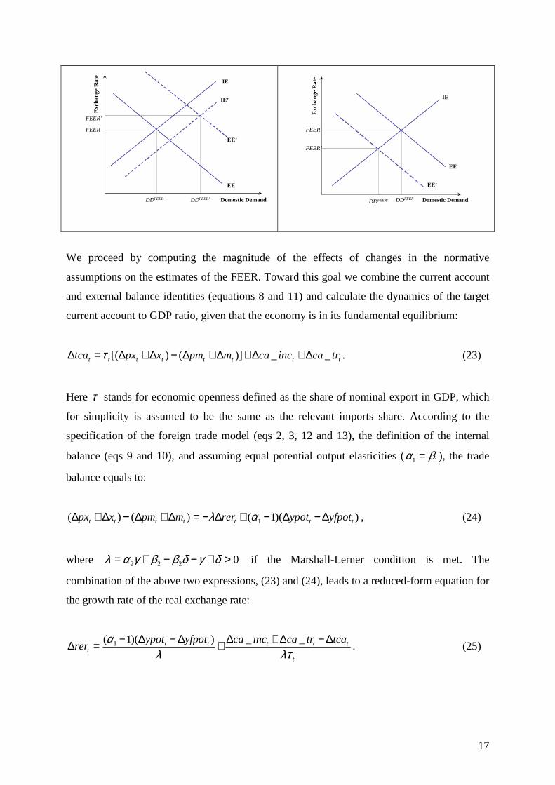
Figure 5. Sensitivity analysis

higher potential output at home higher target current account

17

IE’

EE

Domestic Demand

Exc

hang

e R

ate

DDFEER’

FEER’

IE

DDFEER

FEER

EE’

IE

EE

Domestic Demand

Exc

hang

e R

ate

DDFEER

FEER

EE’

DDFEER’

FEER’

We proceed by computing the magnitude of the effects of changes in the normative

assumptions on the estimates of the FEER. Toward this goal we combine the current account

and external balance identities (equations 8 and 11) and calculate the dynamics of the target

current account to GDP ratio, given that the economy is in its fundamental equilibrium:

tttttttt trcainccampmxpxtca __)]()[( ∆+∆+∆+∆−∆+∆=∆ τ . (23)

Here τ stands for economic openness defined as the share of nominal export in GDP, which

for simplicity is assumed to be the same as the relevant imports share. According to the

specification of the foreign trade model (eqs 2, 3, 12 and 13), the definition of the internal

balance (eqs 9 and 10), and assuming equal potential output elasticities ( 11 βα = ), the trade

balance equals to:

))(1()()( 1 ttttttt yfpotypotrermpmxpx ∆−∆−+∆−=∆+∆−∆+∆ αλ , (24)

where 0222 >+−−+= δγδββγαλ if the Marshall-Lerner condition is met. The

combination of the above two expressions, (23) and (24), leads to a reduced-form equation for

the growth rate of the real exchange rate:

t

tttttt

tcatrcainccayfpotypotrer

λτλα ∆−∆+∆+∆−∆−=∆ __))(1( 1 . (25)

18

Substituting the parameters of the above relationship by their estimates, and taking into

account that in 2008:1 the openess coefficient τ was equal to 0.43, we can calculate that:

)__(24.3)(52.1 tttttt tcatrcainccayfpotypotrer ∆−∆+∆+∆−∆=∆ . (26)

This means that an increase in the assumed level of domestic (foreign) potential output by 1%

appreciates (depreciates) the real exchange rate of the Polish zloty by 1.52%. The results also

show that an increase in the assumed level of the target current account, or a decrease in the

balance on current transfers, by 1% of GDP required in 2008:1 a real depreciation of the zloty

by 3.24%. It should be noticed that the above semi-elasticity is changing over time, depending

on the level of trade openness of the Polish economy.

6. A comparison of the FEER and the BEER

In this section we argue that by including potential output into the specification of the foreign

trade equations of the FEER model we can derive the reduced form-equation for the real

exchange rate that encompasses a standard specification of the BEER relationship, as

proposed by the Clark and MacDonald (1998). According to their specification, the medium-

term value of the real exchange rate is a function of three fundamentals: the terms of trade

(TOT), net foreign assets to GDP ratio and some measure of the Balassa-Samuelson effect

(BS):

tttMT

t totbbsrer 3210 ϑϑϑϑ +++= , (27)

where 0>iϑ for i=1,2,3. We also show that if the openness of the country concerned is not

constant over time, the relationship between the real exchange rate and net foreign assets to

GDP ratio is non-linear. For that reason we argue that the ratio of net foreign assets to trade

value should be used as an explanatory variable in single-equation models for the real

exchange rate, as in Faruquee (1995). Finally, we demonstrate that if our specification of the

foreign trade model is correct, the inclusion of the terms of trade into a set of explanatory

variables in the specification of the BEER model might lead to coefficients indeterminacy.

We start the derivation of the reduced form-equation for the real exchange rate by combining

equations (21) and (22) and calculating the dynamics of the target current account:

19

1)( −∆−−∆+∆=∆ tt byptca κρ . (28)

We proceed by assuming that the income balance is equal to interest payments on net foreign

assets, and thereby:

1_ −∆×=∆ tt biincca , (29)

where i stands for nominal interest rate. Finally, on the basis of relationships (12) and (13) we

compute that the terms of trade are a linear function of the real exchange rate:

tt rertot )( δγ −= . (30)

Substituting the three above expressions to equation (25) yields the following relationship:

tt

ttt

ttt trcatotbyfpotypotrer _)()](1[ 431

213 ∆+∆+∆+∆−∆=∆−− − τ

ϕϕτϕϕδγϕ , (31)

where λαϕ /)1( 11 −= , λκρϕ /)(2 ypi ∆−∆−++= , φ3 is undetermined and λϕ /14 = . As a

result, the reduced form equation for the real exchange rate is:

+++−

−−+= −

t

tt

t

tttt

trcatot

byfpotypotrer

τϕϕ

τϕϕ

δγϕϕ _

)()(1

143

121

30 . (32)

Assuming that the relative potential output is a good approximation of the Balassa-Samuelson

effect7, and that the trade openness and current transfer balance are stable over time, the above

expression is the same as the one proposed by Clark and MacDonald (eq. 27). However, as

the parameter 3ϕ is not uniquely determined, any estimates of the coefficient 3ϑ different

from zero might result in an erroneous interpretation of estimates for 1ϑ and 2ϑ , the

parameters of the BEER model described by relationship (27).

7 In his seminar paper Balassa (1964) uses relative output per capita as a good approximation of relative productivity.

20

7. Conclusions

The application of the FEER model in modeling central and eastern European economies has

been as far considered subject to many shortcomings, primarily due to the fact that changes in

productivity were not accounted for in this approach, whereas the catching-up process is one

of the central arguments of the equilibrium exchange rate appreciation in CEECs. We have

addressed this issue by including potential output in the specification of the foreign trade

equations. As a result, contrary to the standard FEER specification, in our model real

convergence is leading to an appreciation of the real exchange rate. This finding is consistent

with an extensive literature applying the BEER concept in the analysis of CEECs currencies.

Moreover, in this paper we have shown that by including potential output into the

specification of the foreign trade equations of the FEER model one can derive the reduced

form-equation for the real exchange rate that is encompassing the standard specification of the

BEER relationship, as proposed by the Clark and MacDonald (1998). We claim that if the

openness of the country concerned is not constant over time, the single-equation model for the

real exchange rate should take the ratio of net foreign assets to trade value as one of the

explanatory variables. Finally, we have shown that if foreign trade prices are a weighted

average of foreign and domestic prices then the inclusion of the terms of trade into a set of

explanatory variables in the specification of the BEER model might lead to coefficients

indeterminacy. As a result, we argue that the BEER and our version of the FEER should be

considered as substituting approaches to calculate equilibrium exchange rates.

References:

Abiad, Abdul, Daniel Leigh, Ashoka Mody, and Susan Schadler, 2006. Growth in the central and eastern European countries of the European Union, IMF Occasional Papers 252. Aristovnik, Aleksander, 2006. Current account sustainability in selected transition countries, William Davidson Institute Working Paper 844. Armington, Paul S., 1969. A theory of demand for products distinguished by place of production, IMF Staff Papers 16, 159-76. Balassa, Bela. 1964. The purchasing power parity doctrine: A reappraisal, Journal of Political Economy 72, 584-596. Bruha, Jan, and Jiri Podpiera, 2007. Inquiries on dynamics of transition economy convergence in a two-country model, ECB Working Paper 791.

21

Bulíř, Aleš, and Kateřina Šmídková, 2005. Exchange rates in the new EU accession countries: What have we learned from the forerunners? Economic Systems 29(2), 163-186. Bussière, Matthieu, Marcel Fratzscher, and Gernot J. Müller, 2004. Current account dynamics in OECD and EU acceding countries. An intertemporal approach, ECB Working Paper 311. Chinn, Menzie D., and Eswar S. Prasad, 2003. Medium-term determinants of current accounts in industrial and developing countries: An empirical exploration, Journal of International Economics 59, 47-76. Clark, Peter B., and Ronald MacDonald, 1998. Exchange rates and economic fundamentals: A methodological comparison of BEERs and FEERs, IMF Working Paper WP/98/67. Coudert, Virginie, and Cécile Couharde, 2003. Exchange rate regimes and sustainable parities for CEECs in the run-up to EMU membership, Revue Economique 54(5), 983-1012. Debelle, Guy, and Hamid Faruqee, 1996. What determines the current account? A cross-sectional and panel approach, IMF Working Paper WP/96/58. Doisy, Nicolas, and Karine Hervé, 2003. Les deficits courants des PECO: Quelles Implications pour leur entrée dans l´Union Européenne at la zone euro? Economié Internationale 93, 59-88. Driver, Rebecca L., and Simon Wren-Lewis, 1999. FEERs: a sensitivity analysis. In: MacDonald, Ronald, Jerome L. Stein (eds.), Equilibrium Exchange Rates. London: Kluwer Academic Publishers. Égert, Balázs, and Amina Lahrèche-Révil, 2003. Estimating the equilibrium exchange rate of the central and eastern European acceding countries: The challenge of euro adoption, Review of World Economics (Weltwirtschaftliches Archiv) 139(4), 683-708. Égert, Balazs, 2003. Assessing equilibrium exchange rates in CEE acceding countries: Can we have DEER with BEER without FEER? Focus on Transition 2/2003, 38-106. Faruqee, Hamid, 1995. Long-run determinants of the real exchange rate: A stock-flow equilibrium approach, IMF Staff Papers 42, 80-107. Faruqee, Hamid, and Peter Isard, 1998. Exchange rate assessment: Extension of the macroeconomic balance approach, IMF Occassional Paper 167. Fung, San S., and Marc Klau. 2006. The new BIS effective exchange rate indices, BIS Quarterly Review (March), 51-65. Gagnon, Joseph E., 2007, Productive capacity, product varieties, and the elasticities approach to the trade balance, Review of International Economics 15, 639-659. Krugman Paul R., 1989. Differences in income elasticities and trends in real exchange rates, European Economic Review 33, 1055-85.

22

Kwiatkowski, Denis, Peter C. B. Phillips, Peter Schmidt, and Yongcheol Shin, 1992. Testing the null hypothesis of stationary against the alternative of a unit root, Journal of Econometrics 54, 159-178. Lane, Philip R., and Gian Maria Milesi-Ferretti, 2007. Capital flows to central and eastern Europe. Emerging Markets Review 8(2), 106-123. MacKinnon, James G., 1996. Numerical distribution functions for unit root and cointegration tests, Journal of Applied Econometrics 11, 601-618. Maeso-Fernandez, Francisco, Chiara Osbat, and Bernd Schnatz, 2005. Pitfalls in estimating equilibrium exchange rates for transition economies, Economic Systems 29(2), 130-143. Melitz, Marc J., 2003. The impact of trade on intra-industry reallocations and aggregate industry productivity, Econometrica 71(6), 1695-1725. Milesi-Ferretti, Gian Maria, and Assaf Razin. 1996, Sustainability of persistent current account deficits, NBER Working Paper 5467. Ng, Serena, and Pierre Perron, 2001. Lag length selection and the construction of unit root tests with good size and power, Econometrica 69(6), 1519-1552. Rosenberg, Michael R., 1996. Currency Forecasting: A Guide to Fundamental and Technical Models of Exchange Rate Determination. Chicago: IRWIN. Williamson, John, 1994. Estimates of FEER. In: Williamson, John (ed.), Estimating Equilibrium Exchange Rates. Washington: Institute for International Economics. Zanghieri, Paolo, 2004, Current account dynamics in new EU Members: Sustainability and policy issues, CEPII Working Paper 2004-07.