Econometrica, Vol. 79, No. 3 (May, 2011), 733–772

THE GRANULAR ORIGINS OF AGGREGATE FLUCTUATIONS

BY XAVIER GABAIX1

This paper proposes that idiosyncratic firm-level shocks can explain an importantpart of aggregate movements and provide a microfoundation for aggregate shocks. Ex-isting research has focused on using aggregate shocks to explain business cycles, argu-ing that individual firm shocks average out in the aggregate. I show that this argumentbreaks down if the distribution of firm sizes is fat-tailed, as documented empirically.The idiosyncratic movements of the largest 100 firms in the United States appear toexplain about one-third of variations in output growth. This “granular” hypothesis sug-gests new directions for macroeconomic research, in particular that macroeconomicquestions can be clarified by looking at the behavior of large firms. This paper’s ideasand analytical results may also be useful for thinking about the fluctuations of othereconomic aggregates, such as exports or the trade balance.

KEYWORDS: Business cycle, idiosyncratic shocks, productivity, Solow residual, gran-ular residual.

1. INTRODUCTION

THIS PAPER PROPOSES a simple origin of aggregate shocks. It develops the viewthat a large part of aggregate fluctuations arises from idiosyncratic shocks to in-dividual firms. This approach sheds light on a number of issues that are difficultto address in models that postulate aggregate shocks. Although economy-wideshocks (inflation, wars, policy shocks) are no doubt important, they have dif-ficulty explaining most fluctuations (Cochrane (1994)). Often, the explanationfor year-to-year jumps of aggregate quantities is elusive. On the other hand,there is a large amount of anecdotal evidence of the importance of idiosyn-cratic shocks. For instance, the Organization for Economic Cooperation andDevelopment (OECD (2004)) analyzed that, in 2000, Nokia contributed 1.6percentage points of Finland’s gross domestic product (GDP) growth.2 Like-wise, shocks to GDP may stem from a variety of events, such as successful

1For excellent research assistance, I thank Francesco Franco, Jinsook Kim, Farzad Saidi, Hei-wai Tang, Ding Wu, and, particularly, Alex Chinco and Fernando Duarte. For helpful comments,I thank the co-editor, four referees, and seminar participants at Berkeley, Boston University,Brown, Columbia, ECARES, the Federal Reserve Bank of Minneapolis, Harvard, Michigan,MIT, New York University, NBER, Princeton, Toulouse, U.C. Santa Barbara, Yale, the Econo-metric Society, the Stanford Institute for Theoretical Economics, and Kenneth Arrow, RobertBarsky, Susanto Basu, Roland Bénabou, Olivier Blanchard, Ricardo Caballero, David Canning,Andrew Caplin, Thomas Chaney, V. V. Chari, Larry Christiano, Diego Comin, Don Davis, BillDupor, Steve Durlauf, Alex Edmans, Martin Eichenbaum, Eduardo Engel, John Fernald, Je-sus Fernandez-Villaverde, Richard Frankel, Mark Gertler, Robert Hall, John Haltiwanger, ChadJones, Boyan Jovanovic, Finn Kydland, David Laibson, Arnaud Manas, Ellen McGrattan, ToddMitton, Thomas Philippon, Robert Solow, Peter Temin, Jose Tessada, and David Weinstein.I thank for NSF (Grant DMS-0938185) for support.

2The example of Nokia is extreme but may be useful. In 2003, worldwide sales of Nokia were$37 billion, representing 26% of Finland’s GDP of $142 billion. This is not sufficient for a proper

© 2011 The Econometric Society DOI: 10.3982/ECTA8769

734 XAVIER GABAIX

FIGURE 1.—Sum of the sales of the top 50 and 100 non-oil firms in Compustat, as a fractionof GDP. Hulten’s theorem (Appendix B) motivates the use of sales rather than value added.

innovations by Walmart, the difficulties of a Japanese bank, new exports byBoeing, and a strike at General Motors.3

Since modern economies are dominated by large firms, idiosyncratic shocksto these firms can lead to nontrivial aggregate shocks. For instance, in Korea,the top two firms (Samsung and Hyundai) together account for 35% of ex-ports, and the sales of those two firms account for 22% of Korean GDP (diGiovanni and Levchenko (2009)). In Japan, the top 10 firms account for 35%of exports (Canals, Gabaix, Vilarrubia, and Weinstein (2007)). For the UnitedStates, Figure 1 reports the total sales of the top 50 and 100 firms as a fractionof GDP. On average, the sales of the top 50 firms are 24% of GDP, while thesales of the top 100 firms are 29% of GDP. The top 100 firms hence represent alarge part of the macroeconomic activity, so understanding their actions offersgood insight into the aggregate economy.

In this view, many economic fluctuations are not, primitively, due to smalldiffuse shocks that directly affect every firm. Instead, many economic fluctua-tions are attributable to the incompressible “grains” of economic activity, the

assessment of Nokia’s importance, but gives some order of magnitude, as the Finnish base ofNokia is an important residual claimant of the fluctuations of Nokia International.

3Other aggregates are affected as well. For instance, in December 2004, a $24 billion one-timeMicrosoft dividend boosted growth in personal income from 0.6% to 3.7% (Bureau of EconomicAnalysis, January 31, 2005). A macroeconomist would find it difficult to explain this jump inpersonal income without examining individual firm behavior.

GRANULAR ORIGINS OF AGGREGATE FLUCTUATIONS 735

large firms. I call this view the “granular” hypothesis. In the granular view,idiosyncratic shocks to large firms have the potential to generate nontrivial ag-gregate shocks that affect GDP, and via general equilibrium, all firms.

The granular hypothesis offers a microfoundation for the aggregate shocksof real business cycle models (Kydland and Prescott (1982)). Hence, real busi-ness cycle shocks are not, at heart, mysterious “aggregate productivity shocks”or “a measure of our ignorance” (Abramovitz (1956)). Instead, they are welldefined shocks to individual firms. The granular hypothesis sheds light on anumber of other issues, such as the dependence of the amplitude of GDPfluctuations on GDP level, the microeconomic composition of GDP, and thedistribution of GDP and firm-level fluctuations.

In most of this paper, the standard deviation of the percentage growth rateof a firm is assumed to be independent of its size.4 This explains why individualfirms can matter in the aggregate. If Walmart doubles its number of supermar-kets and thus its size, its variance is not divided by 2—as would be the case ifWalmart were the amalgamation of many independent supermarkets. Instead,the newly acquired supermarkets inherit the Walmart shocks, and the total per-centage variance of Walmart does not change. This paper conceptualizes theseshocks as productivity growth, but the analysis holds for other shocks.5

The main argument is summarized as follows. First, it is critical to show that1/

√N diversification does not occur in an economy with a fat-tailed distrib-

ution of firms. A simple diversification argument shows that, in an economywith N firms with independent shocks, aggregate fluctuations should have asize proportional to 1/

√N . Given that modern economies can have millions

of firms, this suggests that idiosyncratic fluctuations will have a negligible ag-gregate effect. This paper points out that when firm size is power-law distrib-uted, the conditions under which one derives the central limit theorem breakdown and other mathematics apply (see Appendix A). In the central case ofZipf’s law, aggregate volatility decays according to 1/ lnN , rather than 1/

√N .

The strong 1/√N diversification is replaced by a much milder one that de-

cays according to 1/ lnN . In an economy with a fat-tailed distribution of firms,diversification effects due to country size are quite small.

Having established that idiosyncratic shocks do not die out in the aggre-gate, I show that they are of the correct order of magnitude to explain businesscycles. We will see that if firm i has a productivity shock dπi, these shocks

4The benchmark that the variance of the percentage growth rate is approximately independentof size (“Gibrat’s law” for variances) appears to hold to a good first degree; see Section 2.5.

5The productivity shocks can come from a decision of the firm’s research department, of thefirm’s chief executive officer, of how to process shipments, inventories, or which new line of prod-ucts to try. They can also stem from changes in capacity utilization, and, particularly, strikes.Suppose a firm, which uses only capital and labor, is on strike for half the year. For many pur-poses, its effective productivity that year is halved. This paper does not require the productivityshocks to arise from any particular source.

736 XAVIER GABAIX

are independent and identically distributed (i.i.d.) and there is no amplifica-tion mechanism, then the standard deviation of total factor productivity (TFP)growth is σTFP = σπh, where σπ is the standard deviation of the i.i.d. pro-ductivity shocks and h is the sales herfindahl of the economy. Using the es-timate of annual productivity volatility of σπ = 12% and the sales herfindahlof h = 5�3% for the United States in 2008, one predicts a TFP volatility equalto σTFP = 12% · 5�3% = 0�63%. Standard amplification mechanisms generatethe order of magnitude of business cycle fluctuations, σGDP = 1�7%. Non-U.S.data lead to even larger business cycle fluctuations. I conclude that idiosyn-cratic granular volatility seems quantitatively large enough to matter at themacroeconomic level.

Section 3 then investigates accordingly the proportion of aggregate shocksthat can be accounted for by idiosyncratic fluctuations. I construct the “granu-lar residual” Γt , which is a parsimonious measure of the shocks to the top 100firms:

Γt :=K∑i=1

salesi�t−1

GDPt−1(git − gt)�

where git − gt is a simple measure of the idiosyncratic shock to firm i. Regress-ing the growth rate of GDP on the granular residual yields an R2 of roughlyone-third. Prima facie, this means that idiosyncratic shocks to the top 100 firmsin the United States can explain one-third of the fluctuations of GDP. More so-phisticated controls for common shocks confirm this finding. In addition, thegranular residual turns out to be a useful novel predictor of GDP growth whichcomplements existing predictors. This supports the view that thinking aboutfirm-level shocks can improve our understanding of GDP movements.

Previous economists have proposed mechanisms that generate macroeco-nomic shocks from purely microeconomic causes. A pioneering paper is byJovanovic (1987), whose models generate nonvanishing aggregate fluctuationsowing to a multiplier proportional to

√N , the square root of the number

of firms. However, Jovanovic’s theoretical multiplier of√N � 1000 is much

larger than is empirically plausible.6 Nonetheless, Jovanovic’s model spawned alively intellectual quest. Durlauf (1993) generated macroeconomic uncertaintywith idiosyncratic shocks and local interactions between firms. The drivers ofhis results are the nonlinear interactions between firms, while in this paperit is the skewed distribution of firms. Bak, Chen, Scheinkman, and Woodford(1993) applied the physical theory of self-organizing criticality. While there ismuch to learn from their approach, it generates fluctuations more fat-tailedthan in reality, with infinite means. Nirei (2006) proposed a model where ag-gregate fluctuations arise from (s� S) rules at the firm level, in the spirit of Bak

6If the actual multiplier were so large, the impact of trade shocks, for instance, would be muchhigher than we observe.

GRANULAR ORIGINS OF AGGREGATE FLUCTUATIONS 737

et al. (1993). These models are conceptually innovative, but they are hard towork with theoretically and empirically. The mechanism proposed in this paperis tractable and relies on readily observable quantities.

Long and Plosser (1983) suggested that sectoral (rather than firm) shocksmight account for GDP fluctuations. As their model has a small number ofsectors, those shocks can be viewed as miniaggregate shocks. Horvath (2000),as well as Conley and Dupor (2003), explored this hypothesis further. Theyfound that sector-specific shocks are an important source of aggregate volatil-ity. Finally, Horvath (1998) and Dupor (1999) debated whether N sectors canhave a volatility that does not decay according to 1/

√N . I found an alternative

solution to their debate, which is formalized in Proposition 2. My approach re-lies on those earlier contributions and clarifies that the fat-tailed nature of thesectoral shocks is important theoretically, as it determines whether the centrallimit theorem applies.

Studies disagree somewhat on the relative importance of sector-specificshocks, aggregate shocks, and complementarities. Caballero, Engel, and Halti-wanger (1997) found that aggregate shocks are important, while Horvath(1998) concluded that sector-specific shocks go a long way toward explainingaggregate disturbances. Many of these effects in this paper could be expressedin terms of sectors.

Granular effects are likely to be even stronger outside the United States, asthe United States is more diversified than most other countries. One numberreported in the literature is the value of the assets controlled by the richest10 families, divided by GDP. Claessens, Djankov, and Lang (2000) found anumber equal to 38% in Asia, including 84% of GDP in Hong Kong, 76% inMalaysia, and 39% in Thailand. Faccio and Lang (2002) also found that thetop 10 families control 21% of listed assets in their sample of European firms.It would be interesting to transpose the present analysis to those countries andto entities other than firms—for instance, business groups or sectors.

This paper is organized as follows. Section 2 develops a simple model. It alsoprovides a calibration that indicates that the effects are of the right order ofmagnitude to account for macroeconomic fluctuations. Section 3 shows directlythat the idiosyncratic movements of firms appear to explain, year by year, aboutone-third of actual fluctuations in GDP, and also contains a narrative of thegranular residual and GDP. Section 4 concludes.

2. THE CORE IDEA

2.1. A Simple “Islands” Economy

This section uses a concise model to illustrate the idea. I consider an islandseconomy with N firms. Production is exogenous, like in an endowment econ-

738 XAVIER GABAIX

omy, and there are no linkages between firms (those will be added later). Firmi produces a quantity Sit of the consumption good. It experiences a growth rate

�Si�t+1

Sit

= Si�t+1 − Sit

Sit

= σiεi�t+1�(1)

where σi is firm i’s volatility and εi�t+1 are uncorrelated random variables withmean 0 and variance 1. Firm i produces a homogeneous good without anyfactor input. Total GDP is

Yt =N∑i=1

Sit(2)

and GDP growth is

�Yt+1

Yt

= 1Yt

N∑i=1

�Si�t+1 =N∑i=1

σi

Sit

Yt

εi�t+1�

As the shocks εi�t+1 are uncorrelated, the standard deviation of GDP growth isσGDP = (var �Yt+1

Yt)1/2:

σGDP =(

N∑i=1

σ2i ·

(Sit

Yt

)2)1/2

�(3)

Hence, the variance of GDP, σ2GDP, is the weighted sum of the variance σ2

i ofidiosyncratic shocks with weights equal to ( Sit

Yt)2, the squared share of output

that firm i accounts for. If the firms all have the same volatility σi = σ , weobtain

σGDP = σh�(4)

where h is the square root of the sales herfindahl of the economy:

h =[

N∑i=1

(Sit

Yt

)2]1/2

�(5)

For simplicity, h will be referred to as the herfindahl of the economy.This paper works first with the basic model (1)–(2). The arguments apply if

general equilibrium mechanisms are added.

GRANULAR ORIGINS OF AGGREGATE FLUCTUATIONS 739

2.2. The 1/√N Argument for the Irrelevance of Idiosyncratic Shocks

Macroeconomists often appeal to aggregate (or at least sectorwide) shocks,since idiosyncratic fluctuations disappear in the aggregate if there is a largenumber of firms N . Consider firms of initially identical size equal to 1/N ofGDP and identical standard deviation σi = σ . Then (4)–(5) gives:

σGDP = σ√N�

To estimate the order of magnitude of the cumulative effect of idiosyncraticshocks, take an estimate of firm volatility σ = 12% from Section 2.4 and con-sider an economy with N = 106 firms.7 Then

σGDP = σ√N

= 12%103

= 0�012% per year.

Such a GDP volatility of 0�012% is much too small to account for the em-pirically measured size of macroeconomic fluctuations of around 1%. This iswhy economists typically appeal to aggregate shocks. More general modellingassumptions predict a 1/

√N scaling, as shown by the next proposition.

PROPOSITION 1: Consider an islands economy with N firms whose sizes aredrawn from a distribution with finite variance. Suppose that they all have the samevolatility σ . Then the economy’s GDP volatility follows, as N → ∞

σGDP ∼ E[S2]1/2

E[S]σ√N�(6)

PROOF: Since σGDP = σh, I examine h: N1/2h = (N−1 ∑Ni=1 S

2i )

1/2

N−1 ∑Ni=1 Si

. The law of

large numbers ensures that N−1∑N

i=1 S2i

a�s�→ E[S2] and N−1∑N

i=1 Sia�s�→ E[S]. This

yields N1/2ha�s�→ E[S2]1/2/E[S]. Q.E.D.

Proposition 1 will be contrasted with Proposition 2 below, which shows thatdifferent models of the size distribution of firms lead to dramatically differentresults.

2.3. The Failure of the 1/√N Argument When

the Firm Size Distribution Is Power Law

The firm size distribution, however, is not thin-tailed, as assumed in Propo-sition 1. Indeed, Axtell (2001), using Census data, found a power law with ex-ponent ζ = 1�059 ± 0�054. Hence, the size distribution of U.S. firms is well

7Axtell (2001) reported that in 1997 there were 5.5 million firms in the United States.

740 XAVIER GABAIX

approximated by the power law with exponent ζ = 1, the “Zipf” distribution(Zipf (1949)). This finding holds internationally, and the origins of this distrib-ution are becoming better understood (see Gabaix (2009)). The next proposi-tion examines behavior under a “fat-tailed” distribution of firms.

PROPOSITION 2: Consider a series of island economies indexed by N ≥ 1.Economy N has N firms whose growth rate volatility is σ and whose sizesS1� � � � � SN are drawn from a power law distribution

P(S > x) = ax−ζ(7)

for x > a1/ζ , with exponent ζ ≥ 1. Then, as N → ∞, GDP volatility follows

σGDP ∼ vζ

lnNσ for ζ = 1�(8)

σGDP ∼ vζ

N1−1/ζσ for 1 < ζ < 2�(9)

σGDP ∼ vζ

N1/2σ for ζ ≥ 2�(10)

where vζ is a random variable. The distribution of vζ does not depend on N and σ .When ζ ≤ 2, vζ is the square root of a stable Lévy distribution with exponent ζ/2.When ζ > 2, vζ is simply a constant. In other terms, when ζ = 1 (Zipf ’s law),GDP volatility decays like 1/ lnN rather than 1/

√N .

In the above proposition, an expression like σGDP ∼ vζ

N1−1/ζ σ means σGDP ×N1−1/ζ converges to vζσ in distribution. More formally, for a series of randomvariables XN and of positive numbers aN , XN ∼ aNY means that XN/aN

d→ Y

as N → ∞, whered→ is the convergence in distribution.

I comment on the economics of Proposition 2 before proving it. The firm sizedistribution has thin tails, that is, finite variance, if and only if ζ > 2. Proposi-tion 1 states that if the firm size distribution has thin tails, then σGDP decaysaccording to 1/

√N . In contrast, Proposition 2 states that if the firm size distri-

bution has fat tails (ζ < 2), then σGDP decays much more slowly than 1/√N : it

decays as 1/N1−1/ζ .To get the intuition for the scaling, take the case a = 1 and observe that (7)

implies that “typical” size S1 of the largest firm is such that S−ζ1 = 1/N , hence

S1 = N1/ζ (see Sornette (2006) for that type of intuition). In contrast, GDP isY � NE[S] when ζ > 1 by the law of large numbers. Hence, the share of thelargest firm is S1/Y = N−(1−1/ζ)/E[S] ∝ N−(1−1/ζ):8 this is a small decay when

8Here f (Y) ∝ g(Y) for some functions f�g means that the ratio f (Y)/g(Y) tends, for largeY , to be a positive real number. So f and g have the same scaling “up to a constant factor.”

GRANULAR ORIGINS OF AGGREGATE FLUCTUATIONS 741

ζ is close to 1. Likewise, the size of the top k firms satisfies S−ζk = k/N , so

Sk = (N/k)1/ζ . Hence, the share of the largest K firms (for a fixed K) is pro-portional to N−(1−1/ζ). Plugging this into (5), we see that the herfindahl, andGDP volatility, is proportional to N−(1−1/ζ).

In the case ζ = 1, E[S] = ∞, so GDP cannot be Y � NE[S]. The followingheuristic reasoning gives the correct value. As firm size density is x−2 and wesaw that the largest firm has typical size N , the typical average firm size is SN =∫ N

1 x−2xdx = lnN , and then Y � NSN = N lnN . Hence, the share of the topfirm is S1/Y = 1/ lnN . By the above reasoning, GDP volatility is proportionalto 1/ lnN .

The perspective of Proposition 2 is that of an economist who knows the GDPof various countries, but not the size of their respective firms, except that, forinstance, they follow Zipf’s law. Then he would conclude that the volatilityof a country of size N should be proportional to 1/ lnN . This explains the vζterms in the distribution of σGDP: when ζ < 2, GDP volatility (and the herfind-ahl h) depends on the specific realization of the size distribution of top firms.Because of the fat-tailedness of the distribution of firms, σGDP does not havea degenerate distribution even as N → ∞. For the same reason, when ζ > 2,the law of large numbers applies and the distribution of volatility does becomedegenerate. Of course, if the economist knows the actual size of the firms, thenshe could calculate the standard deviation of GDP directly by calculating theherfindahl index. Note also that as GDP is made of some large firms, GDPfluctuations are typically not Gaussian (mathematically, the Lindeberg–Fellertheorem does not apply, because there are some large firms). The ex ante dis-tribution is developed further in Proposition 3.

Having made these remarks about the meaning of Proposition 2, let mepresent its proof.

PROOF OF PROPOSITION 2: Since σGDP = σh, I examine

h =N−1

(N∑i=1

S2i

)1/2

N−1N∑i=1

Si

�(11)

I observe that when ζ > 1, the law of large numbers gives

N−1N∑i=1

Si → E[S](12)

742 XAVIER GABAIX

almost surely, so

h ∼N−1

(N∑i=1

S2i

)1/2

E[S] �

I will first complete the above heuristic proof for the scaling as a function N ,which will be useful to ground the intuition, and then present a formal proofwhich relies on the heavier machinery of Lévy’s theorem.

Heuristic Proof. For simplicity, I normalize a = 1. I observe that the size ofthe ith largest firm is approximately

Si�N =(

i

N

)−1/ζ

�(13)

The reason for (13) is the following. As the counter-cumulative distributionfunction (CDF) of the distribution is x−ζ , the random variable S−ζ followsa uniform distribution. Hence, the size of firm number i out of N followsE[S−ζ

i�N] = i/(N + 1). So in a heuristic sense, we have S−ζi�N � i/(N + 1) or, more

simply, (13).From representation (13), the herfindahl can be calculated as

hN ∼N−1+1/ζ

(N∑i=1

i−2/ζ

)1/2

E[S] �

In the fat-tailed case, ζ < 2, the series∑∞

i=1 i−2/ζ converges, hence

hN ∼N−1+1/ζ

( ∞∑i=1

i−2/ζ

)1/2

E[S] = CN−1+1/ζ

for a constant C . Volatility scales as N−1+1/ζ , as in (9).In contrast, in the finite-variance case, the series

∑∞i=1 i

−2/ζ diverges and wehave

∑N

i=1 i−2/ζ ∼ ∫ N

1 i−2/ζ di ∼ N1−2/ζ/(1 − 2/ζ), so that

hN ∼ N−1+1/ζ(N1−2/ζ/(1 − 2/ζ))1/2

E[S] = C ′N−1/2�

and as expected volatility scales as N−1/2.

GRANULAR ORIGINS OF AGGREGATE FLUCTUATIONS 743

Rigorous Proof. When ζ > 2, the variance of firm sizes is finite and I useProposition 1. When ζ ≤ 2, I observe that S2

i has power-law exponent ζ/2 ≤ 1,as shown by

P(S2 > x)= P(S > x1/2

) = a(x1/2

)−ζ = ax−ζ/2�

So to handle the numerator of (11), I use Lévy’s theorem from Appendix A.This implies

N−2/ζN∑i=1

S2i

d→ u�

where u is a Lévy-distributed random variable with exponent ζ/2. So whenζ ∈ (1�2], I can use the fact (12) to conclude

N1−1/ζh =

(N−2/ζ

N∑i=1

S2i

)1/2

N−1N∑i=1

Si

d→ u1/2

E[S] �

When ζ = 1, additional care is required, because E[S] = ∞. Lévy’s theoremapplied to Xi = Si gives aN =N and bN =N lnN , hence

1N

(N∑i=1

Si −N lnN

)d→ g�

where g follows a Lévy distribution with exponent 1, which implies

Y =N∑i=1

Si ∼N lnN�(14)

I conclude h ∼ u1/2/ lnN . Q.E.D.

I conclude with a few remarks. Proposition 2 offers a resolution to the debatebetween Horvath (1998, 2000) and Dupor (1999). Horvath submited evidencethat sectoral shocks may be enough to generate aggregate fluctuations. Du-por (1999) debated this on theoretical grounds and claimed that Horvath wasable to generate large aggregate fluctuations only because he used a moderatenumber of sectors (N = 36). If he had many more finely disaggregated sectors(e.g., 100 times as many), then aggregate volatility would decrease in 1/

√N

(e.g., 10 times smaller). Proposition 2 illustrates that both viewpoints are cor-rect, but apply in different settings. Dupor’s reasoning holds only in a world

744 XAVIER GABAIX

of small firms, when the central limit theorem can apply. Horvath’s empiricalworld is one where the size distribution of firms is sufficiently fat-tailed that thecentral limit theorem does not apply. Instead, Proposition 2 applies and GDPvolatility remains substantial even if the number N of subunits is large.

Though the benchmark case of Zipf’s law is empirically relevant, and the-oretically clean and appealing, many arguments in this paper do not dependon it. The results only require that the herfindahl of actual economies is suffi-ciently large. For instance, if the distribution of firm sizes were lognormal witha sufficiently high variance, then quantitatively very little would change.

The herfindahls generated by a Zipf distribution are reasonably high. ForN = 106 firms, with an equal distribution of sizes, h = 1/

√N = 0�1%� but in

a Zipf world with ζ = 1, Monte Carlo simulations show that the median h =12%. With a firm volatility of σ = 12%, this corresponds to a GDP volatilityσh of 0.012% for identically sized firms and a more respectable 1.4% for aZipf distribution of firm sizes. This is the theory under the Zipf benchmark,which has a claim to hold across countries and clarifies what we can expectindependently of the imperfections of data sets and data collection.

2.4. Can Granular Effects Be Large Enough in Practice? A Calibration

I now examine how large we can expect granular effects to be. For greater re-alism, I incorporate two extra features compared to the island economy: input–output linkages and the endogenous response in inputs to initial disturbances.I start with the impact of linkages.

2.4.1. Economies With Linkages

Consider an economy with N competitive firms buying intermediary inputsfrom one another. Let firm i have Hicks-neutral productivity growth dπi. Hul-ten (1978) showed that the increase in aggregate TFP is9

dTFPTFP

=∑i

sales of firm i

GDPdπi�(15)

This formula shows that, somewhat surprisingly, we can calculate TFPshocks without knowing the input–output matrix: the sufficient statistic for theimpact of firm i is its size, as measured by its sales (i.e., gross output rather thannet output). This helps simplify the analysis.10 In addition, the weights add upto more than 1. This reflects the fact that productivity growth of 1% in a firm

9For completeness, Appendix B rederives and generalizes Hulten’s theorem.10However, to study the propagation of shocks and the origin of size, the input–output matrix

can be very useful. See Carvalho (2009) and Acemoglu, Ozdaglar, and Tahbaz-Salehi (2010), whostudied granular effects in the economy viewed as a network.

GRANULAR ORIGINS OF AGGREGATE FLUCTUATIONS 745

generates an increase in produced values equal to 1% times its sales, not timesits sales net of inputs (which would be the value added). The firm’s sales arethe proper statistic for that social value.

I now draw the implications for TFP volatility. Suppose productivity shocksdπi are uncorrelated with variance σ2

π . Then the variance of productivitygrowth is

vardTFPTFP

=∑i

(sales of firm i

GDP

)2

var(dπi)(16)

and so the volatility of the growth of TFP is

σTFP = hσπ�(17)

where h is the sales herfindahl,

h =(

N∑i=1

(salesitGDPt

)2)1/2

�(18)

I now examine the empirical magnitude of the key terms in (17), startingwith σπ .

2.4.2. Large Firms Are Very Volatile

Most estimates of plant-level volatility find very large volatilities of salesand employment, with an order of magnitude σ = 30–50% per year (e.g.,Caballero, Engel, and Haltiwanger (1997), Davis, Haltiwanger, and Schuh(1996)). Also, the volatility of firm size in Compustat is a very large, 40% peryear (Comin and Mullani (2006)). Here I focus the analysis on the top 100firms. Measuring firm volatility is difficult, because various frictions and identi-fying assumptions provide conflicting predictions about links between changesin total factor productivity and changes in observable quantities such as salesand employment. I consider the volatility of three measures of growth rates:� ln(salesit/employeesit), � ln salesit , and � ln employeesit . For each measureand each year, I calculate the cross-sectional variance among the top 100 firmsof the previous year and take the average.11 I find standard deviations of 12%,12%, and 14% for, respectively, growth rates of the sales per employee, ofsales, and of employees. Also, among the top 100 firms, the sample correla-tions are 0.023, 0.073, and 0.033, respectively, for each of the three measures.12

11In other terms, for each year t, I calculate the cross-sectional variance of growth rates, σ2t =

K−1 ∑Ki=1 g

2it − (K−1 ∑K

i=1 git)2, with K = 100. The corresponding average standard deviation is

[T−1 ∑Tt=1 σ

2t ]1/2.

12For each year, we measure the sample correlation ρt = [ 1K(K−1)

∑i �=j gitgjt ]/[ 1

K

∑i g

2it], with

K = 100. The correlations are positive. Note that a view that would attribute the major firm-level

746 XAVIER GABAIX

Hence, the correlation between growth rates is small. At the firm level, mostvariation is idiosyncratic.

In conclusion, the top 100 firms have a volatility of 12% based on sales peremployee. In what follows, I use σπ = 12% per year for firm-level volatility asthe baseline estimate.

2.4.3. Herfindahls and Induced Volatility

I next consider the impact of endogenous factor usage on GDP. Calling ΛTFP, many models predict that when there are no other disturbances, GDPgrowth dY/Y is proportional to TFP growth dΛ/Λ: dY/Y = μdΛ/Λ for someμ≥ 1 that reflects factor usage; alternatively, via (15),

dY

Y= μ

∑i

sales of firm i

Ydπi�(19)

This gives a volatility of GDP equal to σGDP = μσTFP, and via (17),

σGDP = μσπh�(20)

To examine the size of μ, I consider a few benchmarks. In a short-term modelwhere capital is fixed in the short run and the Frisch elasticity of labor supplyis φ, μ = 1/(1 − αφ/(1 + φ)), and if the supply of capital is flexible (e.g., viavariable utilization or the current account), then μ = (1 + φ)/α.13 With aneffective Frisch elasticity of 2 (as recommend by Hall (2009) for an inclusiveelasticity that includes movements in and out of the labor force), those valuesare μ = 1�8 and μ = 4�5. If TFP is a geometrical random walk, in the neoclas-sical growth model where only capital can be accumulated, in the long run, wehave μ = 1/α, where α is the labor share; with α = 2/3, this gives μ = 1�5.14

I use the average of the three above values, μ= 2�6.Empirically, the sales herfindahl h is quite large: h = 5�3% for the United

States in 2008 and h = 22% in an average over all countries.15 This means,parenthetically, that the United States is a country with relatively small firms(compared to GDP), where the granular hypothesis might be the hardest toestablish.

movements to shocks to the relative demand for a firm’s product compared to its competitorswould counterfactually predict a negative correlation.

13This can be seen by solving maxL ΛK1−αLα −L1+1/φ or maxK�L ΛK1−αLα − rK −L1+1/φ, re-spectively, which gives Y ∝ Λμ for the announced value of μ. For this derivation, I use the localrepresentation with a quasilinear utility function, but the result does not depend on that.

14If Yt = ΛtK1−αt Lα, Λt ∝ eγt , and capital is accumulated, then in a balanced growth path,

Yt ∝Kt ∝Λ1/αt . This holds also with stochastic growth.

15The U.S. data are from Compustat. The international herfindahls are from Acemoglu, John-son, and Mitton (2009). They analyzed the Dun and Bradstreet data set, which has a good cover-age of the major firms in many countries, though not a complete or homogeneous one.

GRANULAR ORIGINS OF AGGREGATE FLUCTUATIONS 747

I can now incorporate all those numbers, using σπ = 12% seen above. Equa-tion 20 yields a GDP volatility σGDP = 2�6×12%×5�3% = 1�7% for the UnitedStates, and σGDP = 2�6 × 12% × 22% = 6�8% for a typical country. This is verymuch on the order of magnitude of GDP fluctuations. As always, further am-plification mechanisms can increase the estimate. I conclude that idiosyncraticvolatility seems quantitatively large enough to matter at the macroeconomiclevel.

2.5. Extension: GDP Volatility When the Volatility of a Firm Depends on Its Size

I now study the case where the volatility of a firm’s percentage growthrate decreases with firm size, which will confirm the robustness of the pre-vious results and yield additional predictions. I examine the functional formσfirm(S)= kS−α from (21). If α> 0, then large firms have a smaller standard de-viation than small firms. Stanley, Amaral, Buldyrev, Havlin, Leschhorn, Maass,Salinger, and Stanley (1996) quantified the relation more precisely and showedthat (21) holds for firms in Compustat, with α� 1/6.

It is unclear whether the conclusions from Compustat can generalize to thewhole economy. Compustat only comprises firms traded on the stock marketand these are probably more volatile than nontraded firms, as small volatilefirms are more prone to seek outside equity financing, while large firms arein any case very likely to be listed in the stock market. This selection bias im-plies that the value of α measured from Compustat firms alone is presumablylarger than in a sample composed of all firms. It is indeed possible α may be 0when estimated on a sample that includes all firms, as random growth modelshave long postulated. In any case, any deviations from Gibrat’s law for vari-ances appear to be small, that is, 0 ≤ α ≤ 1/6. If there is no diversification assize increases, then α = 0. If there is full diversification and a firm of size S iscomposed of S units, then α = 1/2. Empirically, firms are much closer to theGibrat benchmark of no diversification, α= 0.

The next proposition extends Propositions 1 and 2 to the case where firmvolatility decreases with firm size.

PROPOSITION 3: Consider an islands economy, with N firms that have power-law distribution P(S > x)= (Smin/x)

ζ for ζ ∈ [1�∞). Assume that the volatility ofa firm of size S is

σfirm(S)= σ

(S

Smin

)−α

(21)

for some α ≥ 0 and the growth rate is �S/S = σfirm(S)u, where E[u] = 0. Defineζ ′ = ζ/(1 − α) and α′ = min(1 − 1/ζ ′�1/2), so that α′ = 1/2 for ζ ′ ≥ 2. GDPfluctuations have the following form. If ζ > 1,

�Y

Y∼N−α′ ζ − 1

ζE[|u|ζ′ ]1/ζ′

σgζ′� if ζ ′ < 2�(22)

748 XAVIER GABAIX

�Y

Y∼ N−α′ ζ − 1

ζ

E[S2σfirm(S)2]1/2E[u2]1/2

Sming2� if ζ ′ ≥ 2�(23)

where gζ′ is a standard Lévy distribution with exponent ζ ′. Recall that g2 is simplya standard Gaussian distribution. If ζ = 1,

�Y

Y∼ N−α′

lnNE[|ε|ζ′ ]1/ζ′

σgζ′� if ζ ′ < 2�(24)

�Y

Y∼ N−α′

lnN

E[S2σfirm(S)2]1/2E[u2]1/2

Sming2� if ζ ′ ≥ 2�(25)

In particular, the volatility σ(Y) of GDP growth decreases as a power-law func-tion of GDP Y ,

σGDP(Y) ∝ Y−α′�(26)

To see the intuition for Proposition 3, we apply the case of Zipf’s law (ζ = 1)to an example with two large countries, 1 and 2, in which country 2 has twice asmany firms as country 1. Its largest K firms are twice as large as the largest firmsof country 1. However, scaling according to (21) implies that their volatility is2−α times the volatility of firms in country 1. Hence, the volatility of country2’s GDP is 2−α times the volatility of country 1’s GDP (i.e., (26)). Putting thisanother way, under the case presented by Proposition 3 and ζ = 1, large firmsare less volatile than small firms (equation (21)). The top firms in big countriesare larger (in an absolute sense) than top firms in small countries. As the topfirms determine a country’s volatility, big countries have less volatile GDP thansmall countries (equation (26)).

Also, one can reinterpret Proposition 3 by interpreting a large firm as a“country” made up of smaller entities. If these entities follow a power-law dis-tribution, then Proposition 3 applies and predicts that the fluctuations of thegrowth rate � lnSit , once rescaled by S−α

it , follow a Lévy distribution with ex-ponent min{ζ/(1 − α)�2}. Lee, Amaral, Meyer, Canning, and Stanley (1998)plotted this empirical distribution, which looks roughly like a Lévy stable dis-tribution. It could be that the fat-tailed distribution of firm growth comes fromthe fat-tailed distribution of the subcomponents of a firm.16

A corollary of Proposition 3 may be worth highlighting.

COROLLARY 1—Similar Scaling of Firms and Countries: When Zipf ’s lawholds (ζ = 1) and α≤ 1/2, we have α′ = α, that is, firms and countries should seetheir volatility scale with a similar exponent:

σfirms(S)∝ S−α� σGDP(Y) ∝ Y−α�(27)

16See Sutton (2002) for a related model, and Wyart and Bouchaud (2003) for a related analysis,which acknowledges the contribution of the present article, which was first circulated in 2001.

GRANULAR ORIGINS OF AGGREGATE FLUCTUATIONS 749

Interestingly, Lee et al. (1998) presented evidence that supports (27), with asmall exponent α� 1/6 (see also Koren and Tenreyro (2007)). A more system-atic investigation of this issue would be interesting.

Finally, Proposition 3 adopts the point of view of an economist who wouldnot know the sizes of firms in the country. Then the best guess is a Lévy dis-tribution of GDP fluctuations. However, given precise knowledge of the sizeof firms, GDP fluctuations will depend on the details of the distribution of themicroeconomic shocks ui.

Before concluding this theoretical section, let me touch on another verysalient feature of business cycles: firms and sectors comove. As seen by Longand Plosser (1983), models with production and demand linkages can gener-ate comovement. Carvalho and Gabaix (2010) worked out such a model withpurely idiosyncratic shocks and demand linkages. In that economy, the equilib-rium growth rates of sales, employees, and labor productivity can be expressedas

git = aεit + bft� ft ≡N∑j=1

Sj�t−1

Yt−1εjt�(28)

where εit is the firm idiosyncratic productivity shock. Hence, the economy is aone-factor model, but, crucially, the common factor ft is nothing but a sum ofthe idiosyncratic firm shocks. In their calibration, over 90% of output variancewill be attributed to comovement, as in the empirical findings of Shea (2002).Hence, a calibrated granular model with linkages and only idiosyncratic shocksmay account for a realistic amount of comovement. This arguably good featureof granular economies generates econometric challenges, as we shall now see.

3. TENTATIVE EMPIRICAL EVIDENCE FROM THE GRANULAR RESIDUAL

3.1. The Granular Residual: Motivation and Definition

This section presents tentative evidence that the idiosyncratic movements ofthe top 100 firms explain an important fraction (one-third) of the movementof total factor productivity (TFP). The key challenge is to identify idiosyncraticshocks. Large firms could be volatile because of aggregate shocks, rather thanthe other way around. There is no general solution for this “reflection prob-lem” (Manski (1993)). I use a variety of ways to measure the share of idiosyn-cratic shocks.

I start with a parsimonious proxy for the labor productivity of firm i, the logof its sales per worker:

zit := lnsales of firm i in year t

number of employees of firm i in year t�(29)

This measure is selected because it requires only basic data that are more likelyto be available for non-U.S. countries, unlike more sophisticated measures

750 XAVIER GABAIX

such as a firm-level Solow residual. Most studies that construct productivitymeasures from Compustat data use (29). I define the productivity growth rateas git = zit − zit−1. Various models (including the one in the National Bureauof Economic Research (NBER) working paper version of this article) predictthat, indeed, the productivity growth rate is closely related to git .

Suppose that productivity evolves as

git = β′Xit + εit�(30)

where Xit is a vector of factors that may depend on firm characteristics at timet−1 and on factors at time t (e.g., as in equation (28)). My goal is to investigatewhether εit , the idiosyncratic component of the total factor productivity growthrate of large firms, can explain aggregate TFP. More precisely, I would liketo empirically approximate the ideal granular residual Γ ∗

t , which is the directrewriting of (15):

Γ ∗t :=

K∑i=1

Si�t−1

Yt−1εit �(31)

It is the sum of idiosyncratic firm shocks, weighted by size. I wish to see whatfraction of the total variance of GDP growth comes from the granular residual,as the theory (19) predicts that GDP growth is gYt = μΓ ∗

t .I need to extract εit . To do so, I estimate (30) for the top Q ≥ K firms of the

previous year, on a vector of observables that I will soon specify. I then formthe estimate of idiosyncratic firm-level productivity shock as ε̂it = git − β̂′Xit .I define the “granular residual” Γt as

Γt :=K∑i=1

Si�t−1

Yt−1ε̂it �(32)

Identification is achieved if the measured granular residual Γt is close to theideal granular residual Γ ∗

t .Two particularizations are useful, because they do not demand much data

and are transparent. They turn out to do virtually as well as the more com-plicated procedures I will also consider. The simplest specification is to con-trol for the mean growth rate in the sample, that is, to have Xit = gt , wheregt =Q−1

∑Q

i=1 git . Here, I take the average over the top Q firms. We could haveQ = K or take the average over more firms. In practice, I will calculate thegranular residual over the top K = 100 firms, but take the averages for thecontrols over the top Q = 100 or 1000 firms. Then the granular residual is theweighted sum of the firm’s growth rate minus the average firm growth rate:

Γt =K∑i=1

Si�t−1

Yt−1(git − gt)�(33)

GRANULAR ORIGINS OF AGGREGATE FLUCTUATIONS 751

Another specification is to control for the mean growth gIit, the equal-

weighted average productivity growth rate among firms that are in i’s industryand among the top Q firms therein. Then Xit = gIit

. That gives

Γt =K∑i=1

Si�t−1

Yt−1

(git − gIit

)�(34)

It is the weighted sum of the firm growth rates minus the growth rates of otherfirms in the same industry. The term git −gIit

may be closer to the ideal εit thangit − gt , as gIit

may control better than gt for industry-wide disturbances, forexamples, industry-wide real price movements.

Before that, I state a result that establishes sufficient conditions for identifi-cation.

PROPOSITION 4: Suppose that (i) decomposition (30) holds with a vector ofobservables Xit and that (ii)

∑∞i=1(

Si�t−1Yt−1

)2E[|Xit |2] < ∞. Then, as the number of

firms becomes large (in K or in Q ≥ K), Γt(K�Q) − Γ ∗t (K) → 0 almost surely,

that is, the empirical granular residual Γt is close to the ideal granular residual Γ ∗t .

Assumption (i) is the substantial one. Given that in practice I will have Xit

made of gt and gIit, and their interaction with firm size, I effectively assume

that the average growth rate of firms and their industries, perhaps interactedwith the firm size or such nonlinear transformation of it, span the vector offactors. In other terms, firms within a given industry respond in the same wayto common shocks or respond in a way that is related to firm size as in (36)below. This is the case under many models, but they are not fully general. In-deed, without some sort of parametric restriction, there is no solution (Manski(1993)). A typical problematic situation would be the case where the top firmhas a high loading on industry factors that is not captured by its size. Then,instead of the large firms affecting the common factor, the factor would affectthe large firms. However, I do control for size and the interaction between sizeand industry, and aggregate effects, so in that sense I can hope to be reasonablysafe.17

Assumption (ii) is simply technical and is easily verified. For instance, it isverified if E[X2

it] is finite and the herfindahl is bounded. Formally, the herfind-ahl (which, as we have seen, is small anyway) is bounded if the total sales to out-

17The above reflects my best attempt with Compustat data. Suppose one had continuous-timefirm-level data and could measure the beginning of a strike, the launch of a new product, orthe sales of a big export contract. These events would be firm-level shocks. It would presumablytake some time to reverberate in the rest of the economy. Hence, a more precise understandingwould be achieved. Perhaps future data (e.g., using newspapers to approximate continuous-timeinformation) will be able to systematically achieve this extra measure of identification via the timeseries.

752 XAVIER GABAIX

put ratio is bounded by some amount B, as∑∞

i=1(Si�t−1Yt−1

)2 ≤ (∑∞

i=1Si�t−1Yt−1

)2 ≤ B2.Note that here we do not need to assume a finite number of firms, and that inpractice B � 2 (Jorgensen, Gollop, and Fraumeni (1987)).

To complete the econometric discussion, let me also mention a small samplebias: The R2 measured by a regression will be lower than the true R2, becausethe control by gt effectively creates an error in variables problem. This effect,which can be rather large (and biases the results against the granular hypothe-sis), is detailed in the Supplemental Material (Gabaix (2011)).

I would like to conclude with a simple economic example that illustrates thebasic granular residual (equation (33)).18 Suppose that the economy is madeof one big firm which produces half of output, and a million other very smallfirms, and that I have good data on 100 firms: the big firm and the top 99 largestof the very small firms. The standard deviation of all growth rates is 10%, andgrowth rates are given by git =Xt + εit , where Xt is a common shock. Supposethat, in a given year, GDP increases by 3% and that the big firm has growthof, say, 6%, while the average of the small ones is close to 0%. What can weinfer about the origins of shocks? If one thinks of all this being generated by anaggregate shock of 3%, then the distribution of implied idiosyncratic shocks is3% for the big firm and −3% on average for all small ones. The probability thatthe average of the i.i.d. small firms is −3%, given the law of large numbers forthese firms, is very small. Hence, it is more likely that the average shock Xt isaround 0%, and the economy-wide growth of 3% comes from an idiosyncraticshock to the large firm equal to 6%. The estimate of the aggregate shock iscaptured by gt , which is close to 0%, and the estimate of the contribution ofidiosyncratic shocks is captured by the granular residual, Γ = 3%.

3.2. Empirical Implementation

3.2.1. Basic Specification

I use annual U.S. Compustat data from 1951 to 2008. For the granular resid-ual, I take the K = 100 largest firms in Compustat according to the previousyear’s sales that have valid sales and employee data for both the current andprevious years and that are not in the oil, energy, or finance sectors.19 Indus-tries are three-digit Standard Industrial Classification (SIC) codes. Compus-tat contains some large outliers, which may result from extraordinary events,

18I thank Olivier Blanchard for this example.19For firms in the oil/energy sector, the wild swings in worldwide energy prices make (29) too

poor a proxy of total factor productivity. Likewise, the “sales” of financial firms do not meshwell with the meaning (“gross output”) used in the present paper; this exclusion has little impact,though is theoretically cleaner.

GRANULAR ORIGINS OF AGGREGATE FLUCTUATIONS 753

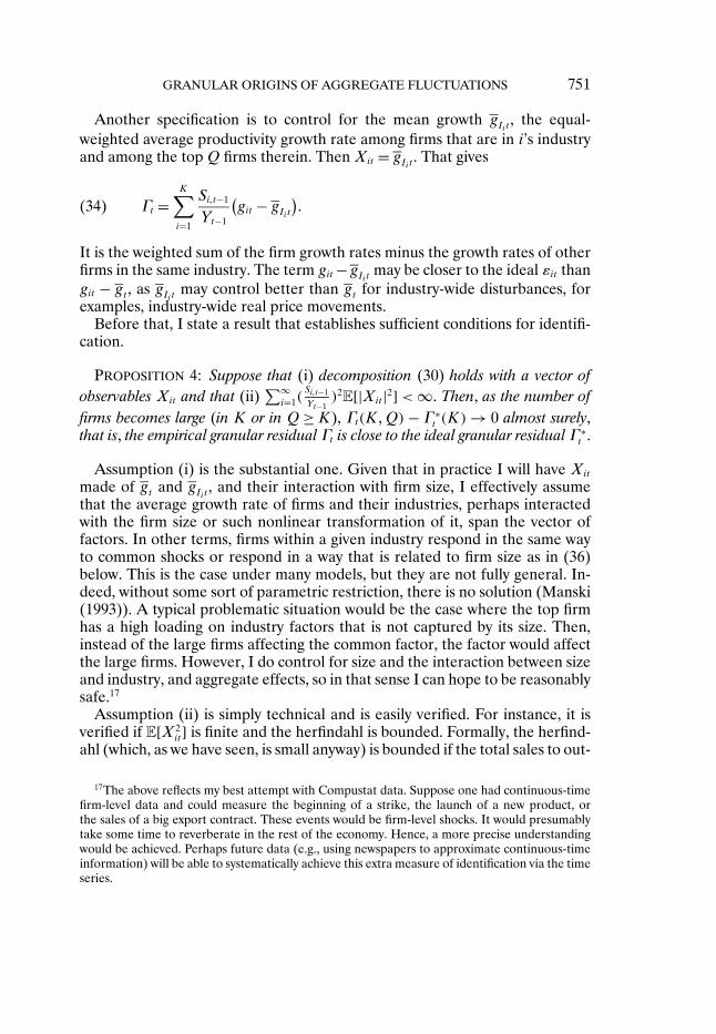
TABLE I

EXPLANATORY POWER OF THE GRANULAR RESIDUALa

GDP Growtht Solowt

(Intercept) 0.018** 0.017** 0.011** 0.01**(0.0026) (0.0025) (0.002) (0.0021)

Γt 1.8* 2.5** 2.1** 2.3**(0.69) (0.69) (0.54) (0.57)

Γt−1 2.6** 2.9** 1.2* 1.3*(0.71) (0.67) (0.55) (0.56)

Γt−2 2.1** 0.65(0.71) (0.59)

N 56 55 56 55R2 0.266 0.382 0.261 0.281Adj. R2 0.239 0.346 0.233 0.239

aFor the year t = 1952 to 2008, per capita GDP growth and the Solow residual areregressed on the granular residual Γt of the top 100 firms (equation (33)). The firms arethe largest by sales of the previous year. Standard errors are given in parentheses.

such as a merger. To handle these outliers, I winsorize the extreme demeanedgrowth rates at 20%.20

Table I presents regressions of GDP growth and the Solow residual on thesimplest granular residual (33). These regressions are supportive of the gran-ular hypothesis. The R2’s are reasonably high, at 34�6% for the GDP growthand around 23�9% for the Solow residual when using two lags. We will soonsee that the industry-demeaned granular residual does even better.

If only aggregate shocks were important, then the R2 of the regressions in Ta-ble I would be zero. Hence, the good explanatory power of the granular resid-ual is inconsistent with a representative firm framework. It is also inconsistentwith the hypothesis that most firm-level volatility might be due to a zero-sumredistribution of market shares.

Let us now examine the results if we incorporate a more fine-grained controlfor industry shocks.

3.2.2. Controlling for Industry Shocks

I next control for industry shocks, that is, use specification (34). Table IIpresents the results, which are consistent with those in Table I. The adjusted

20For instance, I construct (32) by winsorizing ε̂it at M = 20%, that is by replacing it by T (̂εit),where T(x) = x if |x| ≤ M , and T(x) = sign(x)M if |x| >M . I use M = 20%, but results are notmaterially sensitive to the choice of that threshold.

754 XAVIER GABAIX

TABLE II

EXPLANATORY POWER OF THE GRANULAR RESIDUAL WITHINDUSTRY DEMEANINGa

GDP Growtht Solowt

(Intercept) 0.019** 0.017** 0.011** 0.011**(0.0024) (0.0022) (0.0019) (0.0019)

Γt 3.4** 4.5** 3.3** 3.7**(0.86) (0.82) (0.68) (0.72)

Γt−1 3.4** 4.3** 1.5* 1.9**(0.82) (0.78) (0.65) (0.68)

Γt−2 2.7** 0.77(0.79) (0.69)

N 56 55 56 55R2 0.356 0.506 0.334 0.372Adj. R2 0.332 0.477 0.309 0.335

aFor the year t = 1952 to 2008, per capita GDP growth and the Solow residual areregressed on the granular residual Γt of the top 100 firms (equation (34)), removing theindustry mean within this top 100. The firms are the largest by sales of the previous year.Standard errors are given in parentheses.

R2’s are a bit higher: about 47�7% for GDP growth and 33�5% for the Solowresidual when using two lags.21

This table reinforces the conclusion that idiosyncratic movements of the top100 firms seem to explain a large fraction (about one-third, depending on thespecification) of GDP fluctuations. In addition, industry controls, which may bepreferable to a single aggregate control on a priori grounds, slightly strengthenthe explanatory power of the granular residual.

In terms of economics, Tables I and II indicate that the lagged granularresidual helps explain GDP growth, and that the same-year “multiplier” μ isaround 3.

3.2.3. Predicting GDP Growth With the Granular Residual

The above regressions attempt to explain GDP with the granular residual,that is, relating aggregate movement to contemporary firm-level idiosyncraticmovements that may be more easily understood (as we will see in the narrativebelow). I now study forecasting GDP growth with past variables. In addition tothe granular residual, I consider the main traditional predictors. I control foroil and monetary policy shocks by following the work of Hamilton (2003) andRomer and Romer (2004), which are arguably the leading way to control for oiland monetary policy shocks. I also include the 3-month nominal T-bill and the

21The similarity of the results is not surprising, as the correlation between the simple andindustry-demeaned granular residual is 0�82.

GRANULAR ORIGINS OF AGGREGATE FLUCTUATIONS 755

TABLE III

PREDICTIVE POWER OF THE GRANULAR RESIDUAL FOR TERM SPREAD,OIL SHOCKS, AND MONETARY SHOCKSa

1 2 3 4 5 6 7 8

(Intercept) 0.022** 0.02** 0.022** 0.026** 0.015 0.015 0.019** 0.021**(0.0029) (0.0029) (0.0029) (0.0057) (0.0075) (0.0079) (0.0027) (0.0073)

Oilt−1 −0.00027* −0.00024* −8.7e−05 −0.00017(0.00012) (0.00012) (0.00013) (0.00012)

Oilt−2 −0.00018 −0.00017 −6.9e−05 −0.00012(0.00012) (0.00012) (0.00012) (0.00011)

Monetaryt−1 −0.083 −0.08 −0.042 −0.051(0.057) (0.055) (0.055) (0.05)

Monetaryt−2 −0.059 −0.038 −0.024 0.043(0.057) (0.056) (0.054) (0.053)

rt−1 −0.75** −0.6 −0.45 −0.41(0.2) (0.32) (0.37) (0.34)

rt−2 0.65** 0.56 0.43 0.39(0.19) (0.32) (0.37) (0.34)

Term spreadt−1 0.32 0.38 0.4(0.6) (0.64) (0.58)

Term spreadt−2 0.45 0.27 −0.38(0.47) (0.54) (0.53)

Γt−1 3.5** 3.3**(0.96) (1)

Γt−2 1.2 2.3*(0.92) (0.97)

N 55 55 55 55 55 55 55 55R2 0.121 0.0764 0.175 0.22 0.288 0.312 0.215 0.463Adj. R2 0.0871 0.0409 0.109 0.191 0.231 0.192 0.185 0.341

aFor the year t = 1952 to 2008, per capita GDP growth is regressed on the lagged values of the granular residualΓt of the top 100 firms (equation (34)), of the Hamilton (for oil) and Romer–Romer (for money) shocks, and theterm spread (the government 5-year bond yield minus the 3-month yield). We see that the granular residual has goodincremental predictive power even beyond the term spread. Standard errors are given in parentheses.

term spread (which is defined as the 5-year bond rate minus the 3-month bondrate), which is often found to be the a very good predictor of GDP (those twoendogenous variables are arguably more “diagnostic” than “causal,” though).Table III presents the results.

The granular residual has an adjusted R2 (called R2) equal to 18�5% (col-umn 7). The traditional economic factors—oil and money shocks—have an R2

of 10�9% (column 3). Past GDP growth has a very small R2 of −0�3%, a num-ber not reported in Table III to avoid cluttering the table too much. The tradi-tional diagnostic financial factors—the interest rate and the term spread—havean R2 of 23�1% (column 5). Putting all predictors together, the R2 is 34�1%

756 XAVIER GABAIX

(column 8) and the granular residual brings an incremental R2 of 14�9% (com-pared to column 6).

I conclude that the granular residual is a new and apparently useful predictorof GDP. This result suggests that economists might use the granular residualto improve not only the understanding of GDP, but also its forecasting.

3.3. Robustness Checks

An objection to the granular residual is that the control for the common fac-tors may be imperfect. Table IV shows the explanatory power of the granularresidual, controlling for oil and monetary shocks. The adjusted R2 is 47�7%for the granular residual (column 4), it is 8�2% and 2�3% for oil and monetaryshocks, respectively (columns 1 and 2), and 49�5% for financial variables (in-terest rates and term spread, column 6). To investigate whether the granularresidual does add explanatory power, the last column puts all those variablestogether (perhaps pushing the believable limit of ordinary least squares (OLS)because of the large number of regressors) and shows that the explanatoryvariables yield an R2 of 76�7%.

In conclusion, as a matter of “explaining” (in a statistical sense) GDPgrowth, the granular residual does nearly as well as all traditional factors to-gether, and complements their explanatory power.

I report a few robustness checks in the Supplemental Material. For instance,among the explanatory variables of (30), I include not only gt or gIit

, but alsotheir interaction with log firm size and its square. The impact of the controlfor size is very small. Using a number Q = 1000 of firms yields similar results,too. Finally, I could not regress git on GDP growth at time t because then byconstruction I would eliminate any explanatory power of εit .

I conclude that the granular residual has a good explanatory power for GDP,even controlling for traditional factors. In addition, it has good forecastingpower, complementing other factors. Hence, the granular residual must cap-ture interesting firm-level dynamics that are not well captured by traditionalaggregate factors.

I have done my best to obtain “idiosyncratic” shocks; given that I do not havea clean instrument, the above results should still be considered provisional. Thesituation is the analogue, with smaller stakes, to that of the Solow residual.Solow understood at the outset that there are very strong assumptions in theconstruction of his residual, in particular, full capacity utilization and no fixedcost. But a “purified” Solow residual took decades to construct (e.g., Basu, Fer-nald, and Kimball (2006)), requires much better data, is harder to replicate inother countries, and relies on special assumptions as well. Because of that, theSolow residual still endures, at least as a first pass. In the present paper too, itis good to have a first step in the granular residual, together with caveats thatmay help future research to construct a better residual. The conclusion of thisarticle contains some other measures of granular residuals that build on the

GRANULAR ORIGINS OF AGGREGATE FLUCTUATIONS 757

TABLE IV

EXPLANATORY POWER OF THE GRANULAR RESIDUAL FOROIL AND MONETARY SHOCKS, AND INTEREST RATESa

1 2 3 4 5 6 7 8

(Intercept) 0.023** 0.02** 0.022** 0.017** 0.019** 0.016* 0.02** 0.023**(0.003) (0.0029) (0.003) (0.0022) (0.0023) (0.0065) (0.005) (0.0048)

Oilt −9.8e−05 −8.3e−05 −4.6e−05 −7.9e−05(0.00011) (0.00012) (8.6e−05) (7.5e−05)

Oilt−1 −0.00028* −0.00026* −0.00021* −0.00019*(0.00012) (0.00012) (8.8e−05) (7.5e−05)

Oilt−2 −0.00019 −0.00019 −0.00012 −4.3e−05(0.00012) (0.00012) (8.9e−05) (6.8e−05)

Monetaryt −0.0088 −0.03 −0.057 −0.044(0.059) (0.058) (0.043) (0.032)

Monetaryt−1 −0.08 −0.065 0.012 −0.013(0.061) (0.059) (0.047) (0.033)

Monetaryt−2 −0.061 −0.048 0.031 0.095**(0.059) (0.058) (0.046) (0.033)

Γt 4.5** 4.2** 3.7** 4**(0.82) (0.88) (0.69) (0.66)

Γt−1 4.3** 4.5** 2.8** 3.6**(0.78) (0.85) (0.71) (0.68)

Γt−2 2.7** 2.7** 2.6** 2.8**(0.79) (0.8) (0.69) (0.63)

rt 0.66* 0.69** 0.83**(0.26) (0.2) (0.19)

rt−1 −1.6** −1.5** −1.5**(0.35) (0.28) (0.27)

rt−2 1** 0.85** 0.7**(0.29) (0.23) (0.22)

Term spreadt −0.49 −0.11 −0.13(0.52) (0.41) (0.38)

Term spreadt−1 0.17 −0.34 −0.37(0.52) (0.41) (0.42)

Term spreadt−2 0.31 −0.02 −0.18(0.39) (0.32) (0.33)

N 55 55 55 55 55 55 55 55R2 0.133 0.0768 0.189 0.506 0.582 0.551 0.755 0.832Adj. R2 0.0824 0.0225 0.0878 0.477 0.498 0.495 0.706 0.767

aFor the year t = 1952 to 2008, per capita GDP growth is regressed on the granular residual Γt of the top 100 firms(equation (34)), and the contemporaneous and lagged values of the Hamilton (for oil) shocks, and Romer–Romer(for money) shocks. The firms are the largest by sales of the previous year. Standard errors are given in parentheses.

758 XAVIER GABAIX

present paper. It could be that the recent factor-analytic methods (Stock andWatson (2002), Foerster, Stock, and Watson (2008)) will prove useful for ex-tending the analysis. One difficulty is that the identities of the top firms changeover time, unlike in the typical factor-analytic setup. This said, another wayto understand granular shocks is to examine some of them directly, a task towhich I now turn.

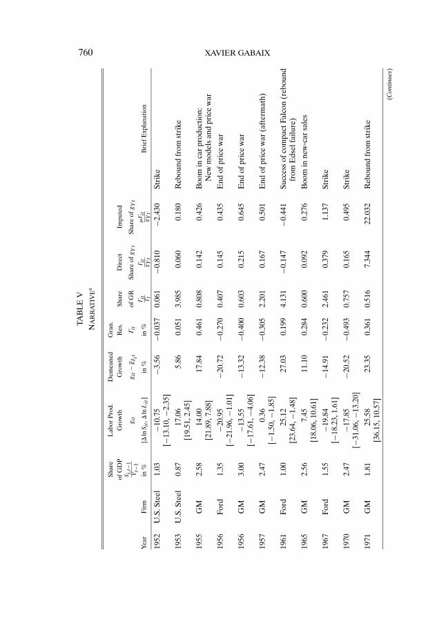
3.4. A Narrative of GDP and the Granular Residual

Figure 2 presents a scatter plot with 3�4Γt + 3�4Γt−1, where the coefficientsare those from Table II. I present a narrative of the most salient events inthat graph.22 Some notations are useful. The firm-specific granular residual(or granular contribution) is defined to be Γit = Si�t−1

Yt−1g′it with g′

it = git − gIit.

The share of the industry-demeaned granular residual (GR) is defined as γit =Γit/Γt , and the share of GDP growth is defined as Γit/gYt , where gYt is thegrowth rate of GDP per capita minus its average value in the sample, for short“demeaned GDP growth.” Given the regression coefficients in Tables I and II,this share should arguably be multiplied by a productivity multiplier μ� 3.

FIGURE 2.—Growth of GDP per capita against 3�4Γt + 3�4Γt−1, the industry-demeaned gran-ular residual and its lagged value. The display of 3�4Γt + 3�4Γt−1 is motivated by Table II, whichyields regression coefficients on Γt and Γt−1 of that magnitude.

22A good source for firm-level information besides Compustat is the web sitefundinguniverse.com, which compiles a well referenced history of the major companies.Google News, the yearly reports of the Council of Economic Advisors, and Temin (1998) are alsouseful.

GRANULAR ORIGINS OF AGGREGATE FLUCTUATIONS 759

To obtain a manageable number of important episodes, I report the eventswith |gYt | ≥ 0�7σY , and in those years, report the firms for which |Γit/gYt | ≥0�14. I also consider all the most extreme fifth of the years for Γt . I avoid, how-ever, most points that are artefacts of mergers and acquisitions (more on thatlater). To avoid boring the reader with too many tales of car companies, I add afew non-car events that I found interesting economically or methodologically.

A general caveat is that the direction of the causality is hard to assess de-finitively, as the controls gIit

for industry-wide movements are imperfect. Withthat caveat in mind, we can start reading Table V.

To interpret the table, let me take a salient and relatively easy year, 1970.This year features a major strike at General Motors, which lasted 10 weeks(September 15 to November 20). The 1970 row of Table V shows that GM’ssales fell by 31% and employment fell by 13%. Its labor productivity growthrate is thus −17�9% and, controlling for the industry mean productivity growthof 2�6% that year, GM’s demeaned growth rate is −20�5%. Given that GM’ssales the previous year were 2.47% of GDP, GM’s granular residual is Γit =−0�20 × 2�47% = −0�49%. That means the direct impact of this GM event is achange in GDP by −0�49% that year. Note also that with a productivity multi-plier of μ� 3, the imputed impact of GM on GDP is −1�47%. As GDP growththat year was 3% below trend (gYt = −3%), the direct share of the GM eventis 0�49%/3% = 0�16 and its full imputed share is 1�47%/3% = 0�49. In somemechanical sense, the GM event appears to account for a fraction 0.17 of theGDP movement directly and, indirectly, for about 0.5 of the GDP innovationthat year. It also accounts for a fraction 0.76 of the granular residual. Hence,it is plausible to interpret 1970 as a granular year, whose salient event was theGM strike and the turmoils around it.23 This example shows how the table isorganized. Let me now present the rest of the narrative.

1952–1953: U.S. Steel faces a strike from about April 1952 to August 1952.U.S. Steel’s production falls by 13.1% in 1952 and rebounds by 19.5% in 1953.The 1953 events explains a share of 3.99 of the granular residual and 0.06 ofexcess GDP growth.

1955 experiences a high GDP growth, and a reasonably high granular resid-ual. The likely microfoundation is a boom in car production. Two main specificfactors seem to explain the car boom: the introduction of new models of carsand the fact that car companies engaged in a price war (Bresnahan (1987)).The car sales of GM increase by 21.9%, while employment increases by 7.9%.The demeaned growth rate is g′

it = 17�8%. GM accounts for 81% of the gran-

23Temin (1998) noted that the winding down of the Vietnam War (which ended in 1975) mayalso be responsible for the slump of 1970. This is in part the case, as during 1968–1972 the ratiosof defense outlays to GDP were 9.5, 8.7, 8.1, 7.3, and 6.7%. On the other hand, the ratio of totalgovernment outlays to GDP were, respectively, 20.6, 19.4, 19.3, 19.5, and 19.6% (source: Councilof Economic Advisors (2005, Table B-79)). Hence the aggregate government spending shock wasvery small in 1970.

760 XAVIER GABAIX

TAB

LE

V

NA

RR

AT

IVE

a

Shar

eL

abor

Prod

.D

emea

ned

Gra

n.of

GD

PG

row

thG

row

thR

es.

Shar

eD

irec

tIm

pute

dSi�t−

1Yt−

1git

git

−gI it

Γit

ofG

RSh

are

ofgYt

Shar

eof

gYt

Yea

rF

irm

in%

[�lnSit

,�lnLit

]in

%in

%Γit Γt

Γit

gYt

μΓit

gYt

Bri

efE

xpla

natio

n

1952

U.S

.Ste

el1.

03−1

0.75

−3.5

6−0

.037

0.06

1−0

.810

−2.4

30St

rike

[−13

.10,

−2.3

5]

1953

U.S

.Ste

el0.

8717

.06

5.86

0.05

13.

985

0.06

00.

180

Reb

ound

from

stri

ke[1

9.51

,2.4

5]

1955

GM

2.58

14.0

017

.84

0.46

10.

808

0.14

20.

426

Boo

min

car

prod

uctio

n:[2

1.89

,7.8

8]N

ewm

odel

san

dpr

ice

war

1956

Ford

1.35

−20.

95−2

0.72

−0.2

700.

407

0.14

50.

435

End

ofpr

ice

war

[−21

.96,

−1.0

1]

1956

GM

3.00

−13.

55−1

3.32

−0.4

000.

603

0.21

50.

645

End

ofpr

ice

war

[−17

.61,

−4.0

6]

1957

GM

2.47

0.36

−12.

38−0

.305

2.20

10.

167

0.50

1E

ndof

pric

ew

ar(a

fter

mat

h)[−

1.50

,−1.

85]

1961

Ford

1.00

25.1

227

.03

0.19

94.

131

−0.1

47−0

.441

Succ

ess

ofco

mpa

ctFa

lcon

(reb

ound

[23.

64,−

1.48

]fr

omE

dsel

failu

re)

1965

GM

2.56

7.45

11.1

00.

284

0.60

00.

092

0.27

6B

oom

inne

w-c

arsa

les

[18.

06,1

0.61

]

1967

Ford

1.55

−19.

84−1

4.91

−0.2

322.

461

0.37

91.

137

Stri

ke[−

18.2

3,1.

61]

1970

GM

2.47

−17.

85−2

0.52

−0.4

930.

757

0.16

50.

495

Stri

ke[−

31.0

6,−1

3.20

]

1971

GM

1.81

25.5

823

.35

0.36

10.

516

7.34

422

.032

Reb

ound

from

stri

ke[3

6.15

,10.

57]

(Con

tinue

s)

GRANULAR ORIGINS OF AGGREGATE FLUCTUATIONS 761TA

BL

EV

—C

ontin

ued

Shar

eL

abor

Prod

.D

emea

ned

Gra

n.of

GD

PG

row

thG

row

thR

es.

Shar

eD

irec

tIm

pute

dSi�t−

1Yt−

1git

git

−gI it

Γit

ofG

RSh

are

ofgYt

Shar

eof

gYt

Yea

rF

irm

in%

[�lnSit

,�lnLit

]in

%in

%Γit Γt

Γit

gYt

μΓit

gYt

Bri

efE

xpla

natio

n

1972

Chr

ysle

r0.

7116

.76

17.8

00.

126

0.23

40.

058

0.17

4R

ush

ofsa

les

for

subc

ompa

cts

[15.

64,−

1.13

](D

odge

Dar

tand

Plym

outh

Val

iant

)

1972

Ford

1.46

14.1

815

.22

0.22

20.

411

0.10

30.

309

Rus

hof

sale

sfo

rsu

bcom

pact

s[1

6.36

,2.1

8](F

ord

Pint

o)

1974

GM

2.59

−11.

31−1

5.23

−0.3

940.

913

0.11

50.

345

Car

sw

ithpo

orga

sm

ileag

ehi

tby

[−21

.28,

−9.9

7]hi

gher

oilp

rice

1983

IBM

b1.

0610

.46

10.5

20.

111

0.17

70.

071

0.21

3L

aunc

hof

the

IBM

PC[1

1.76

,1.2

9]

1987

GE

b0.

7925

.62

21.4

60.

158

1.11

00.

357

1.07

1M

ovin

gou

tofm

anuf

actu

ring

and

[8.3

3,−1

7.29

]in

tofin

ance

and

high

-tec

h

1988

GE

b0.

8321

.42

16.5

50.

137

0.44

10.

117

0.35

1M

ovin

gou

tofm

anuf

actu

ring

and

[20.

08,−

1.33

]in

tofin

ance

and

high

-tec

h

1996

AT

&T

1.08

38.9

732

.45

0.21

50.

471

0.44

61.

338

Spin

-off

ofN

CR

and

Luc

ent

[−44

.11,

−83.

08]

2000

GE

1.20

20.5

633

.04

0.23

99.

934

0.46

81.

404

Sale

sto

pped

$111

bn,e

xpan

sion

ofG

E[1

2.29

,−8.

27]

Med

ical

Syst

ems

2002

Wal

mar

t2.

168.

616.

390.

138

3.21

9−0

.099

−0.2

97Su

cces

sof

lean

dist

ribu

tion

mod

el[9

.83,

1.22

]a G

Ean

dG

Mar

eG

ener

alE

lect

ric

and

Gen

eral

Mot

ors,

resp

ectiv

ely.

For

each

firm

i,git

,�

lnSit

,and

�lnLit

deno

tepr

oduc

tivity

,sal

es,a

ndem

ploy

men

tgr

owth

rate

s,

resp

ectiv

ely,

git

−gI it

deno

tes

indu

stry

-dem

eane

dgr

owth

,and

Si�t−

1/Yt−

1is

the

sale

ssh

are

ofG

DP.

The

firm

gran

ular

resi

dual

isΓit

=Si�t−

1(git

−gI it)

Yt−

1,a

ndΓit/Γ

tis

the

resp

ectiv

esh

are

ofth

egr

anul

arre

sidu

al. Γ

it/g

Yt

isth

edi

rect

shar

eof

the

firm

shoc

kon

dem

eane

dG

DP

grow

th.T

hefu

llsh

are

wou

ldbe

equa

ltoμΓit/g

Yt,

whe

reμ

=3

isth

ety

pica

lpro

duct

ivity

mul

tiplie

res

timat

edfr

omTa

bles

Ian

dII

.b

The

reis

just

one

firm

inth

isin

dust

ryin

the

top

100,

henc

egI it

was

repl

aced

bygt.

762 XAVIER GABAIX

ular residual, a direct fraction 0.14 of excess GDP growth, and an imputedfraction of 0.43 of excess GDP growth.

1956–1957: In 1956, the price war in cars ends, and sales drop back to theirnormal level (the sales of General Motors decline by 17.6%; those of Forddecline by 22%). The granular residual is −0�66%, of which 60% is due toGeneral Motors. Hence, one may provisionally conclude the 1955–1956 boom–bust episode was in large part a granular event driven by new models and aprice war in the car industry.24 In Figure 2, the 56 point is actually the sum of1955 (granular boom) and 1956 (granular bust), and is unremarkable, but thebust is reflected in the 1957 point, which is the most extreme negative point inthe granular residual.

1961: In previous years, Ford cancelled the Edsel brand and introduces togreat success the Falcon, the leading compact car of its time. Ford’s demeanedgrowth rate is g′

it = 27% and its firm granular residual explains a fraction −0�15of excess GDP growth. That is, without Ford’s success, the recession wouldhave been worse.

1965 is an excellent year for GM, with the great popularity of its Chevroletbrand.

1967: Ford experiences a 64-day strike and a terrible year. Its demeanedgrowth rate is −14�9% and its granular residual is −0�23%. It explains a frac-tion 2.5 of the granular residual and 0.38 of GDP growth.

1970 is the GM year described above.1971, which appears in Figure 2 as label “72,” representing the sum of the

granular residuals in 1971 and 1972, is largely characterized by the reboundfrom the negative granular 1970 shock. Hence, the General Motors strikemay explain the very negative 70 (1969 + 1970) point and the very positive72 (1971 + 1972) point. Sales increase by 36.2% and employment increasesby 10.6%. The firm granular residual is Γit = 0�36% for a fraction of granularresidual of 0.52. Another interesting granular event takes place in 1971. TheCouncil of Economic Advisors (1972, p. 33) reports that “prospects of a possi-ble steel strike after July 31st [1971], the expiration day of the labor contracts,caused steel consumers to build up stock in the first seven months of 71, afterwhich these inventories were liquidated.” Here, a granular shock—the possi-bility of a steel strike—creates a large swing in inventories. Without exploringinventories here, one notes that such a plausibly orthogonal inventory shockcould be used in future macroeconomic studies.

1972 is a very good year for Ford and Chrysler. Ford has an enormous successwith its Pinto. At Chrysler, there is a rush of sales for the compact Dodge Dartand Plymouth Valiant (low-priced subcompacts). For those two firms, Γit =0�22% and Γit = 0�13%, respectively.

1974 is probably not a granular year, because the oil shock was commonto many industries. Still, the low value of the granular residual reflects the

24To completely resolve the matter, one would like to control for the effect of the Korean war.

GRANULAR ORIGINS OF AGGREGATE FLUCTUATIONS 763

fact that the top three car companies, and particularly General Motors, weredisproportionately affected by the shock. It is likely that if large companieswere producing more fuel efficient cars, the granular residual would have beencloser to 0, and the slump of 1974 could have been much more moderate. Forinstance, GM’s granular contribution is −0�39%, and its multiplier-adjustedcontribution −1�18%.

1983 is an excellent year for IBM, with the launch of the IBM PC. Its git =10�5%, so that its granular residual is 0�11%.

1987–1988 is an instructive year, in part for methodological reasons. Af-ter various investments and mergers and acquisitions in 1986–1987 (acquisi-tion of financial services providers, e.g., KidderPeabody, and high-tech compa-nies such as medical diagnostics business), the clear majority of GE’s earnings(roughly 80%, compared to 50% 6 years earlier) were generated in servicesand high technology. Its git is 26% and 21% in 1987 and 1988, respectively.Its fraction of the granular residual is 1.11 and 0.44, and its imputed growthfraction is 1.07 and 0.35. This episode can be viewed either as a purely formalreallocation of titles in economic activity (in which case it arguably should bediscarded) or as a movement of “structural change” where this premier firm’sefforts (human and physical) are reallocated toward higher value-added activ-ities, thereby potentially increasing economic activity.25 The same can be saidabout the next event.

1996: There is an intense restructuring at AT&T, with a spin-off of NCR andLucent. AT&T recenters to higher productivity activities, and as a result itsmeasured g′

it is 32.5%. This movement explains a fraction 0.47 of the granularresidual and 0.45 of GDP growth.

2000 is a year of great productivity growth for GE, in particular via the ex-pansion of GE Medical Systems. Its git is 20.6% and its firm granular residualis Γit = 0�24%.

2002 sees a surge in sales for Walmart, a vindication of its lean distribu-tion model. The company’s share of the U.S. GDP in 2001 was 2.2%. This ap-proached the levels reached by GM (3% in 1956) and U.S. Steel Corp. (2.8%in 1917) when these firms were at their respective peaks. Its g′

it is 6�4% and itsfraction of the granular residual is 3.22, while its fraction of demeaned GDPgrowth is −0�10.

We arrive at the limen of the financial crisis. 2007 sees three interesting gran-ular events (not reported in the table) if one is willing to accept the “sales” offinancial firms as face value (it is unclear they should be). The labor productiv-ity growth of AIG, Citigroup, and Merrill Lynch is −15%, −9%, and −25%,respectively, which gives them granular contributions of −0�09%, −0�18%,

25Under the first interpretation, it would be interesting to build a more “purified” granularresidual that filters out corporate finance events. Of course, to what extent those events shouldbe filtered out is debatable.

764 XAVIER GABAIX

and −0�10%. It would be interesting to exploit the hypothesis that the finan-cial crisis was largely caused by the (ex post) mistakes of a few large firms,e.g., Lehman and AIG. Their large leverage and interconnectedness amplifiedinto a full-fledged crisis instead of what could have been a run-of-the-mill thatwould have affected in a diffuse way the financial sector. But doing justice tothis issue would require another paper.

Figure 2 reveals that, in the 1990’s, granular shocks are smaller. Likewise,GDP volatility is smaller—reflecting the “great moderation” explored in theliterature (e.g., McConnell and Perez-Quiros (2000)). Carvalho and Gabaix(2010) explored this link in more depth, and proposed that indeed the decreasein granular volatility explains the great moderation of GDP and its demise.

Finally, the bottom of Figure 2 contains three outliers that are not granularyears. They have conventional “macro” interpretations. 1954 is often attributedto the end of the Korean War, and 1958 and 1982 (the “Volcker recession”) areattributed to tight monetary policy aimed at fighting inflation.

This narrative shows the importance of two types of events: some (e.g., astrike) inherently have a negative autocorrelation, while some others (e.g., newmodels of cars) do not. It is conceivable that forecasting could be improved bytaking into account that distinction.

4. CONCLUSION

This paper shows that the forces of randomness at the microlevel create aninexorable amount of volatility at the macro level. Because of random growthat the microlevel, the distribution of firm sizes is very fat-tailed (Simon (1955),Gabaix (1999), Luttmer (2007)). That fat-tailedness makes the central limittheorem break down, and idiosyncratic shocks to large firms (or, more gener-ally, to large subunits in the economy such as family business groups or sectors)affect aggregate outcomes.

This paper illustrates this effect by taking the example of GDP fluctuations.It argues that idiosyncratic shocks to the top 100 firms explain a large frac-tion (one-third) of aggregate volatility. While aggregate fluctuations such aschanges to monetary, fiscal, and exchange rate policy, and aggregate produc-tivity shocks are clearly important drivers of macroeconomic activity, they arenot the only contributors to GDP fluctuations. Using theory, calibration, anddirect empirical evidence, this paper makes the case that idiosyncratic shocksare an important, and possibly the major, part of the origin of business-cyclefluctuations.

The importance of idiosyncratic shocks in aggregate volatility leads to a num-ber of implications and directions for future research. First, and most evidently,to understand the origins of fluctuations better, one should not focus exclu-sively on aggregate shocks, but concrete shocks to large players, such as Gen-eral Motors, IBM, or Nokia.

Second, shocks to large firms (such as a strike, a new innovation, or a CEOchange), initially independent of the rest of the economy, offer a rich source of

GRANULAR ORIGINS OF AGGREGATE FLUCTUATIONS 765

shocks for vector autoregressions (VARs) and impulse response studies—thereal-side equivalent of the Romer and Romer shocks for monetary economics.As a preliminary step in this direction, the granular residual, with a variety ofspecifications, is available in the Supplemental Material.

Third, this paper gives a new theoretical angle for the propagation of fluc-tuations. If Apple or Walmart innovates, its competitors may suffer in theshort term and thus race to catch up. This creates rich industry-level dynamics(that are already actively studied in the industrial organization literature) thatshould be useful for studying macroeconomic fluctuations, since they allow oneto trace the dynamics of productivity shocks.

Fourth, this argument could explain the reason why people, in practice, donot know the state of the economy. This is because “the state of the econ-omy” depends on the behavior (productivity and investment behavior, amongothers) of many large and interdependent firms. Thus, the integration is noteasy and no readily accessible single number can summarize this state. Thiscontrasts with aggregate measures, such as GDP, which are easily observable.Conversely, agents who focus on aggregate measures may make potentiallyproblematic inferences (see Angeletos and La’O (2010) and Veldkamp andWolfers (2007) for research along those lines). This paper could therefore of-fer a new mechanism for the dynamics of “animal spirits.”

Finally this mechanism might explain a large part of the volatility of many ag-gregate quantities other than output, for instance, inventories, inflation, short-or long-run movements in productivity, and the current account. Fluctuationsof exports due to granular effects are explored in Canals et al. (2007) and diGiovanni and Levchenko (2009). The latter paper in particular finds that low-ering trade barriers increases the granularity of the economy (as the most pro-ductive firms are selected) and implies an increase in the volatility of exports.Blank, Buch, and Neugebauer (2009) constructed a “banking granular resid-ual” and found that negative shocks to large banks negatively impact smallbanks. Malevergne, Santa-Clara, and Sornette (2009) showed that the granu-lar residual of stock returns (the return of a large firm minus a return of theaverage firm) is an important priced factor in the stock market and explainedthe performance of Fama–French factor models. Carvalho and Gabaix (2010)found that the time-series changes in granular volatility predict well the volatil-ity of GDP, including the “great moderation” and its demise.

In sum, this paper suggests that the study of very large firms can offer a usefulangle of attack on some open issues in macroeconomics.

APPENDIX A: LÉVY’S THEOREM

Lévy’s theorem (Durrett (1996, p. 153)) is the counterpart of the central limittheorem for infinite-variance variables.

THEOREM 1—Lévy’s Theorem: Suppose that X1�X2� � � � are i.i.d. with adistribution that satisfies (i) limx→∞ P(X1 > x)/P(|X1| > x) = θ ∈ [0�1] and

766 XAVIER GABAIX

(ii) P(|X1| > x) = x−ζL(x), with ζ ∈ (0�2) and L(x) slowly varying.26 Let sn =∑n

i=1 Xi, an = inf{x : P(|X1| > x) ≤ 1/n}, and bn = nE[X11|X1|≤an]. As n → ∞,(sn − bn)/an converges in distribution to a nondegenerate random variable Y ,which follows a Lévy distribution with exponent ζ.

The most typical use of Lévy’s theorem is the case of a symmetrical distrib-ution with zero mean and power-law distributed tails, P(|X1| > x) ∼ (x/x0)

−ζ .Then an ∼ x0n

1/ζ , bn = 0, and (x0N1/ζ)−1

∑N

i=1 Xid→ Y , where Y follows a Lévy

distribution. The sum∑N

i=1 Xi does not scale as N1/2, as it does in the centrallimit theorem, but it scales as N1/ζ . This is because the size of the largest unitsXi scales as N1/ζ .

A symmetrical Lévy distribution with exponent ζ ∈ (0�2] has the distributionλ(x�ζ) = 1

π

∫ ∞0 e−kζ cos(kx)dk. For ζ = 2, a Lévy distribution is Gaussian. For

ζ < 2, the distribution has a power-law tail with exponent ζ.

APPENDIX B: LONGER DERIVATIONS

PROOF OF PROPOSITION 3: To simplify notations, using homogeneity, I con-sider the case σ = Smin = 1. As �Si/Si = S−α

i ui,

�Y

Y=

N∑i=1

�Si

Y=

N∑i=1

S1−αi ui

N∑i=1

Si

�(35)

When ζ > 1, by the law of large numbers, N−1Y = N−1∑N

i=1 Si → S. Totackle the numerator, I observe that S1−α

i has power-law tails with exponentζ ′ = ζ/(1 − α). I consider two cases. First, if ζ ′ < 2, define xi = S1−α

i ui, whichhas power-law tails with exponent ζ ′, and prefactor given by, for x → ∞,

P(|S1−αi ui| > x) = P

(Si >

(x

|ui|)1/(1−α))

∼ E[|ui|ζ/(1−α)

]x−ζ/(1−α) = E

[|ui|ζ′]x−ζ′

�

Hence in Lévy’s theorem, the aN factor is aN ∼N1/ζ′E[|ui|ζ′ ]1/ζ′ and

�Y =N∑i=1

S1−αi ui ∼N1/ζ′

E[|ui|ζ′]1/ζ′

gζ′�

26L(x) is said to be slowly varying if ∀t > 0� limx→∞ L(tx)/L(x) = 1. Prototypical examples areL(x)= c and L(x) = c lnx for a nonzero constant c.

GRANULAR ORIGINS OF AGGREGATE FLUCTUATIONS 767

where gζ′ is a Lévy with exponent ζ ′. Hence, given S = E[S] = Sminζ/(ζ − 1),

�Y

Y∼ E[|ui|ζ′ ]1/ζ′

N1/ζ′

SNgζ′ = ζ − 1

ζE[|ui|ζ′]1/ζ′

N1/ζ′−1gζ′ �

If ζ ′ = 2, Siσ(Si)ui has finite variance equal to E[S2σ(S)2]E[u2i ]. By the

central limit theorem, �Y ∼ √NE[S2σ(S)2]1/2

E[u2i ]g2, where g2 is a standard

Gaussian distribution and

�Y

Y∼ �Y

NS∼ 1√

N

E[S2σ(S)2]1/2E[u2

i ]1/2

Sg2

as announced. When ζ = 1, a lnN correction appears because of (14), but thereasoning is otherwise the same. Q.E.D.

Hulten’s Theorem With and Without Instantaneous Reallocation of Factors

For clarity, I rederive and extend Hulten’s (1978) result, which says that aHicks-neutral productivity shock dπi to firm i causes an increase in TFP givenby equation (15) (see also Jones (2011) for consequences of this result). Thereare N firms. Firm i produces good i and uses a quantity Xij of intermediary in-puts from firm j. It also uses Li units of labor and Ki units of capital. It has pro-ductivity πi. If production is: Qi = eπiFi(Xi1� � � � �XiN�Li�Ki), the representa-tive agent consumes Ci of good i and has a utility function of U(C1� � � � �CN).Production of firm i serves as consumption and intermediary inputs, so Qi =Ci + ∑

k Xki. The optimum in this economy reads maxCi�Xik�Li�KiU(C1� � � � �CN)

subject to

Ci +∑k

Xki = eπiFi(Xi1� � � � �XiN�Li�Ki);∑i

Li =L;∑i

Ki =K�

The Lagrangian is

W = U(C1� � � � �CN)

+∑i

pi

[eπiFi(Xi1� � � � �XiN�Li�Ki)−Ci −

∑k

Xki

]

+w

[L−

∑i

Li

]+ r

[K −

∑i

Ki

]�

Assume marginal cost pricing. GDP in this economy is Y = wL + rK =∑i piCi. The value added of firm i is wLi + rKi and its sales are piQi.

768 XAVIER GABAIX

If each firm i has a shock dπi to productivity, welfare changes as

dW =∑i

pi[eπiFi(Xi1� � � � �XiN�Li�Ki)dπi]

=∑i

(sales of firm i) dπi�

As dW can be rewritten dW = ∑i∂U∂Ci

dCi = ∑i pi dCi = dY , we obtain equa-

tion (15).The above analysis shows that Hulten’s theorem holds even if, after the

shock, the capital, labor and material inputs are not reallocated. This is a sim-ple consequence of the envelope theorem. Hence Hulten’s result also holds ifthere are frictions in the adjustment of labor, capital, or intermediate inputs.

PROOF OF PROPOSITION 4: We have

Γt(K�Q)− Γ ∗t (K) =

K∑i=1

Si�t−1

Yt−1(̂εit − εit)

=K∑i=1

Si�t−1

Yt

((git − β̂′Xit)− (git −β′Xit))

= (β− β̂)′K∑i=1

Si�t−1

Yt

Xit�

We have β− β̂ → 0 almost surely (a.s.) when K or Q → ∞ (by standard resultson OLS), and

∑K

i=1Si�t−1Yt

Xit → ∑∞i=1

Si�t−1Yt

Xit in the L2 sense by assumption (ii).Hence Γt(K�Q)− Γ ∗

t (K�Q)→ 0 a.s. Q.E.D.

APPENDIX C: DATA APPENDIX

Firm-Level Data

The firm-level data come from the Fundamentals Annual section of theCompustat North America database on WRDS. The data consist of year byfirm observations from 1950 to 2008 of the following variables: SIC code (SIC),net sales in $MM (DATA 12), and employees in M (DATA 29). I exclude for-eign firms based in the United States, restricting the data set to firms whose ficand loc codes are equal to USA. I filter out oil and oil-related companies (SICcodes 2911, 5172, 1311, 4922, 4923, 4924, and 1389), and energy companies(SIC code between 4900 and 4940), as fluctuations of their sales come mostlyfrom worldwide commodity prices, rather than real productivity shocks, and

GRANULAR ORIGINS OF AGGREGATE FLUCTUATIONS 769

financial firms (SIC code between 6000 and 6999), because their sales do notmesh well with the meaning used in the present paper.27

An important caveat is in order for U.S. firms. With Compustat, the salesof Ford, say, represent the worldwide sales of Ford, not directly the outputproduced by Ford in the United States. There is no simple solution to thisproblem, especially if one wants a long time series. An important task of futureresearch is to provide a version of Compustat that corrects for multinationals.

Macroeconomic Data

The real GDP, GDP per capita, and inflation index data series all come fromthe Bureau of Economic Analysis. The Solow residual is the multifactor pro-ductivity of the private business sector reported by the Bureau of Labor Stud-ies. The term spread and real interest rate data are from the Fama–Bliss Centerfor Research in Security Prices (CRSP) Monthly Treasury data base on WRDS.

The data for the Romer and Romer (2004) monetary policy shocks comefrom David Romer’s web page. Their original series (RESID) is monthly from1969 to 1996. Here the yearly Romer–Romer shock is the sum of the 12monthly shocks in that year. For the years not covered by Romer and Romer,the value of the shock is assigned to be 0, the mean of the original data. This as-signment does not bias the regression coefficient under simple conditions, forinstance if the data are i.i.d. It does lower the R2 by the fraction of missed vari-ance; fortunately, most large monetary shocks (e.g., of the 1970’s and 1980’s)are in the data set.

The data for the Hamilton (2003) oil shocks primarily come from JamesHamilton’s web page. This series is quarterly and runs until 2001. It is definedas the amount by which the current oil price exceeds the maximum value overthe past year. This paper’s yearly shock is the sum of the quarterly Hamiltonshocks. The spot price for oil reported by the St. Louis Federal Reserve is usedto extend the series to the present.

REFERENCES

ABRAMOVTIZ, M. (1956): “Resource and Output Trends in the United States Since 1870,” Amer-ican Economic Review, 46, 5–23. [735]

ACEMOGLU, D., S. JOHNSON, AND T. MITTON (2009): “Determinants of Vertical Integration:Financial Development and Contracting Costs,” Journal of Finance, 64, 1251–1290. [746]

ACEMOGLU, D., A. OZDAGLAR, AND A. TAHBAZ-SALEHI (2010): “Cascades in Networks andAggregate Volatility,” Working Paper, MIT. [744]

ANGELETOS, G. M., AND J. LA’O (2010): “Noisy Business Cycles,” in NBER MacroeconomicsAnnual. Cambridge: MIT Press. [765]

AXTELL, R. (2001): “Zipf Distribution of U.S. Firm Sizes,” Science, 293, 1818–1820. [739]

27The results with financial firms are very similar.

770 XAVIER GABAIX

BAK, P., K. CHEN, J. SCHEINKMAN, AND M. WOODFORD (1993): “Aggregate Fluctuations FromIndependent Sectoral Shocks: Self-Organized Criticality in a Model of Production and Inven-tory Dynamics,” Ricerche Economiche, 47, 3–30. [736,737]

BASU, S., J. FERNALD, AND M. KIMBALL (2006): “Are Technology Improvements Contrac-tionary?” American Economic Review, 96, 1418–1448. [756]

BLANK, S., C. BUCH, AND K. NEUGEBAUER (2009): “Shocks at Large Banks and Banking SectorDistress: The Banking Granular Residual,” Discussion Paper 04/2009, Deutsche Bundesbank.[765]

BRESNAHAN, T. (1987): “Competition and Collusion in the American Automobile Market: The1955 Price War,” Journal of Industrial Economics, 35, 457–482. [759]

CABALLERO, R., E. M. R. A. ENGEL, AND J. C. HALTIWANGER (1997): “Aggregate EmploymentDynamics: Building From Microeconomic Evidence,” American Economic Review, 87, 115–137.[737,745]

CANALS, C., X. GABAIX, J. VILARRUBIA, AND D. WEINSTEIN (2007): “Trade Patterns, TradeBalances, and Idiosyncratic Shocks,” Working Paper, Columbia University. [734,765]

CARVALHO, V. (2009): “Aggregate Fluctuations and the Network Structure of IntersectoralTrade,” Working Paper, CREI. [744]

CARVALHO, V., AND X. GABAIX (2010): “The Great Diversification and Its Undoing,” WorkingPaper 16424, NBER. [749,764,765]

CLAESSENS, S., S. DJANKOV, AND L. H. P. LANG (2000): “The Separation of Ownership and Con-trol in East Asian Corporations,” Journal of Financial Economics, 58, 81–112. [737]

COCHRANE, J. (1994): “Shocks,” Carnegie–Rochester Conference Series on Public Policy, 41,295–364. [733]

COMIN, D., AND S. MULANI (2006): “Diverging Trends in Macro and Micro Volatility: Facts,”Review of Economics and Statistics, 88, 374–383. [745]

CONLEY, T., AND B. DUPOR (2003): “A Spatial Analysis of Sectoral Complementarity,” Journalof Political Economy, 111, 311–352. [737]

COUNCIL OF ECONOMIC ADVISORS (1972): Economic Report of the President Transmitted to theCongress. Washington, DC: U.S. Government Printing Office. [762]

(2005): Economic Report of the President Transmitted to the Congress. Washington, DC:U.S. Government Printing Office. [759]

DAVIS, S., J. C. HALTIWANGER, AND S. SCHUH (1996): Job Creation and Destruction. Cambridge,MA: MIT Press. [745]

DI GIOVANNI, J., AND A. LEVCHENKO (2009): “International Trade and Aggregate Fluctuationsin Granular Economies,” Working Paper, University of Michigan. [734,765]

DUPOR, W. (1999): “Aggregation and Irrelevance in Multi-Sector Models,” Journal of MonetaryEconomics, 43, 391–409. [737,743]

DURLAUF, S. (1993): “Non Ergodic Economic Growth,” Review of Economic Studies, 60, 349–366.[736]

DURRETT, R. (1996): Probability: Theory and Examples. Belmont, CA: Wadsworth. [765]FACCIO, M., AND L. H. P. LANG (2002): “The Ultimate Ownership of Western European Corpo-

rations,” Journal of Financial Economics, 65, 365–395. [737]FOERSTER, A., P.-D. SARTE, AND M. WATSON (2008): “Sectoral vs. Aggregate Shocks: A Struc-

tural Factor Analysis of Industrial Production,” Working Paper 08-07, Federal Reserve Bankof Richmond. [758]

GABAIX, X. (1999): “Zipf’s Law for Cities: An Explanation,” Quarterly Journal of Economics, 114,739–767. [764]

(2009): “Power Laws in Economics and Finance,” Annual Review of Economics, 1,255–293. [740]

(2011): “Supplement to ‘The Granular Origins of Aggregate Fluctuations’,” Econo-metrica Supplemental Material, 79, http://www.econometricsociety.org/ecta/Supmat/8769_extensions.pdf; http://www.econometricsociety.org/ecta/Supmat/8769_data and programs.zip.zip. [752]

GRANULAR ORIGINS OF AGGREGATE FLUCTUATIONS 771

HALL, R. (2009): “By How Much Does GDP Rise If the Government Buys More Output?”Brookings Papers on Economic Activity, 2, 183–231. [746]

HAMILTON, J. D. (2003): “What Is an Oil Shock?” Journal of Econometrics, 113, 363–398. [754,769]

HORVATH, M. (1998): “Cyclicality and Sectoral Linkages: Aggregate Fluctuations From SectoralShocks,” Review of Economic Dynamics, 1, 781–808. [737,743]

(2000): “Sectoral Shocks and Aggregate Fluctuations,” Journal of Monetary Economics,45, 69–106. [737,743]

HULTEN, C. (1978): “Growth Accounting With Intermediary Inputs,” Review of Economic Studies,45, 511–518. [744,767]

JONES, C. I. (2011): “Intermediate Goods and Weak Links: A Theory of Economic, Develop-ment,” American Economic Journal: Macroeconomics (forthcoming). [767]

JORGENSON, D. W., F. M. GOLLOP, AND B. M. FRAUMENI (1987): Productivity and U.S. EconomicGrowth. Cambridge, MA: Harvard University Press. [752]

JOVANOVIC, B. (1987): “Micro Shocks and Aggregate Risk,” Quarterly Journal of Economics, 102,395–409. [736]

KOREN, M., AND S. TENREYRO (2007): “Volatility and Development,” Quarterly Journal of Eco-nomics, 122, 243–287. [749]

KYDLAND, F. E., AND E. C. PRESCOTT (1982): “Time to Build and Aggregate Fluctuations,”Econometrica, 50, 1345–1370. [735]

LEE, Y., L. A. N. AMARAL, M. MEYER, D. CANNING, AND H. E. STANLEY (1998): “Univer-sal Features in the Growth Dynamics of Complex Organizations,” Physical Review Letters, 81,3275–3278. [748,749]

LONG, J., AND C. PLOSSER (1983): “Real Business Cycles,” Journal of Political Economy, 91,39–69. [737,749]

LUTTMER, E. G. J. (2007): “Selection, Growth, and the Size Distribution of Firms,” QuarterlyJournal of Economics, 122, 1103–1144. [764]

MALEVERGNE, Y., P. SANTA-CLARA, AND D. SORNETTE (2009): “Professor Zipf Goes to WallStreet,” Working Paper 15295, NBER. [765]

MANSKI, C. F. (1993): “Identification of Endogenous Social Effects: The Reflection Problem,”Review of Economic Studies, 60, 531–542. [749,751]

MCCONNELL, M., AND G. PEREZ-QUIROS (2000): “Output Fluctuations in the United States:What Has Changed Since the Early 1980’s,” American Economic Review, 90, 1464–1476. [764]

NIREI, M. (2006): “Threshold Behavior and Aggregate Critical Fluctuations,” Journal of Eco-nomic Theory, 127, 309–322. [736]

OECD (2004): Economic Survey of Finland, Issue 14. Paris: OECD Publishing. [733]ROMER, C., AND D. ROMER (2004): “A New Measure of Monetary Shocks: Derivation and Im-

plications,” American Economic Review, 94, 1055–1084. [754,769]SHEA, J. (2002): “Complementarities and Comovements,” Journal of Money, Credit and Banking,

42, 412–433. [749]SIMON, H. (1955): “On a Class of Skew Distribution Functions,” Biometrika, 42, 425–440. [764]SORNETTE, D. (2006): Critical Phenomena in Natural Sciences. New York: Springer. [740]STANLEY, M. H. R., L. A. N. AMARAL, S. V. BULDYREV, S. HAVLIN, H. LESCHHORN, P. MAASS,

M. A. SALINGER, AND H. E. STANLEY (1996): “Scaling Behaviour in the Growth of Compa-nies,” Nature, 379, 804–806. [747]

STOCK, J., AND M. WATSON (2002): “Forecasting Using Principal Components From a LargeNumber of Predictors,” Journal of the American Statistical Association, 97, 1167–1179. [758]

SUTTON, J. (2002): “The Variance of Firm Growth Rates: The ‘Scaling’ Puzzle,” Physica A, 312,577–590. [748]

TEMIN, P. (1998): “The Causes of American Business Cycles: An Essay in Economic Historiog-raphy,” in Beyond Shocks, ed. by J. C. Fuhrer and S. Schuh. Boston: Federal Reserve Bank.[758,759]

772 XAVIER GABAIX

VELDKAMP, L., AND J. WOLFERS (2007): “Aggregate Shocks or Aggregate Information? CostlyInformation and Business Cycle Comovement,” Journal of Monetary Economics, 54, 37–55.[765]

WYART, M., AND J.-P. BOUCHAUD (2003): “Statistical Models for Company Growth,” Physica A,326, 241–255. [748]

ZIPF, G. (1949): Human Behavior and the Principle of Least Effort. Cambridge, MA: Addison-Wesley. [740]

Stern School of Finance, New York University, 44 West 4th Street, Suite 9-190,New York, NY 10012, U.S.A. and CEPR and NBER; xgabaix@stern.nyu.edu.

Manuscript received August, 2009; final revision received October, 2010.