ECONOMETRIC FLEXIBILITY IN … FLEXIBILITY IN MICROSIMULATION: AN AGE-CENTRED REGRESSION ... available data set for estimating a model equation is ... the single equation approach

INTERNATIONAL JOURNAL OF MICROSIMULATION (2009) 2(2) 1-14

ECONOMETRIC FLEXIBILITY IN MICROSIMULATION: AN AGE-

CENTRED REGRESSION APPROACH John Sabelhaus1 and Lina Walker2

1Department of Economics, University of Maryland, College Park, Maryland, 20742, and Investment Company Institute, 1401 H Street, NW, Washington, DC, 20005; email: [email protected] 2Public Policy Institute, AARP, Washington, DC. ABSTRACT: This paper describes a strategy for estimating predictive equations that has been shown to work well in microsimulation modelling. The technique, referred to here as ―age-centred regression,‖ is particularly useful when the available data set for estimating a model equation is limited and the marginal effect of one or more explanatory variables might be expected to vary systematically by age. The examples used here to describe how age-centring works are taken

from the labour supply equations in the Congressional Budget Office Long-Term (CBOLT) dynamic microsimulation model. By switching from a traditional single-equation approach to age-centred regression, we show that marginal effects of independent variables can vary significantly across age groups. The comparison also reveals that improvements in mean predictions by age can be

achieved with little if any loss in statistical precision of coefficient estimates.

Keywords: age-centred regression; heterogeneity; spline; kernel 1. INTRODUCTION A fundamental goal of microsimulation modelling is to replicate empirically observed

heterogeneity in person-, household-, or firm-level outcomes. If individuals with certain characteristics are more likely to have certain outcomes, a good model will have transition equations that generate those correlations in simulations. Sample size limitations in the data sets used to estimate model equations

can make achieving this goal a challenge,

however, as they make it difficult to statistically sort out all of the covariance needed to replicate the desired heterogeneity. This paper discusses an estimation strategy, referred to as ―age-centred regression‖, that

has proved useful for mitigating the types of problems in microsimulation that are typically associated with small sample sizes. There are several conditions under which age-centred regression might be useful in microsimulation modelling. First, the

behavioural processes being estimated vary systematically with age: these processes include marital status transitions, fertility, mortality, and labour market outcomes. Second, these processes are such that the

effect of any given explanatory variable could also vary by age: for example, higher

educational attainment might lower the probability of marriage for very young singles, but increase the probability of marriage for middle-aged singles. Third, the data set available for estimating the model equation is limited, so that estimating separate equations

for each age is infeasible and therefore some sort of grouping is required.

A typical approach in microsimulation when these conditions arise is to estimate separate equations for two or more age groups. For instance, in the marital transition equation,

one might estimate separate marriage probability equations for young, middle-aged, and perhaps older individuals, so that the model would have three marriage equations. Age centring takes this grouping approach a step further. The idea is to estimate a separate equation for each unique (or

―reference‖) age, but include every observation

in the sample whose age is within a preset range (or ―bandwidth‖) around the reference age being estimated. Thus, if the sample being analyzed is 25-year-olds and the bandwidth is 4 years, the estimation phase

would use all observations in the data set with ages 21 through 29. The equation for 26-year-olds would use every observation with ages 22 to 30, and so on. The end result is that the model will have separate equations for each reference age, but the sample used to estimate the equation for any given age

overlaps with the data used to estimate nearby ages. There are two benefits when using age-centred regressions, in terms of econometric flexibility.

First, there is flexibility in the shape of the functional form with respect to age itself—one

does not have to rely on polynomial terms or linear splines to specify how the process in question varies with age. Second, the effect of any given independent variable in the equation is no longer constrained to be equal for all age groups (or even a subset of age groups, as

when one splits the sample). If the data suggest that the magnitude or even sign of an

SABELHAUS AND WALKER Econometric flexibility: an age-centred regression approach 2

explanatory variable systematically varies with age, the differential relationship will show up in

the estimates.

The examples used here to illustrate the age-centring approach are taken from the labour force modules in the U.S. Congressional Budget Office Long-Term dynamic microsimulation, also known as CBOLT.1 The equations we consider sequentially predict labour force participation, full-time versus

part-time employment, and hours worked for part-time employed persons. All of the equations are univariate or multinomial logit specifications with standard controls: the explanatory variables include age, marital status, educational attainment, in-school

status, number of children under 6 years of age (for women), receipt of social insurance

benefits, and cohort/time effects. The equations are all estimated using about thirty years of data from the March Current Population Survey (CPS), which is a large, annual, nationally representative cross-section.

For each of the three labour market equations, we compare the results using a standard (linear in age) specification with age-centred results. We show that estimated coefficients in the age-centred equations do vary systematically by age, and those differences in

coefficients imply very different marginal effects by age. One example is the extent to which lagged labour force participation is correlated with current labour force participation; the effect varies systematically

over the life cycle and the age-centred

equation is better able to capture that pattern than the more standard equation. A second example is the effect of marital status on expected part-time hours (conditional on working part-time). The extent to which being married affects part-time hours worked also varies significantly across age groups.

A further benefit of using the age-centred approach in microsimulation modelling is that, by its nature, age-centred regressions are better at capturing any differences in mean predicted outcomes by age. In general, microsimulation modellers rely on the fact that

the single equation approach will work if the underlying outcomes by age are smooth and if

one uses an appropriate polynomial in age. Using the predictions from the labour force module, we show that deviating from those conditions can lead to biased predictions by

age in some cases. 2. THE MECHANICS OF AGE-CENTRED REGRESSION Age-centred regression is useful for estimating

microsimulation model equations in cases where the underlying process varies

systematically by age and one is trying to achieve maximum flexibility in the estimated

econometric relationships. In microsimulation modelling, researchers typically split the sample by age when estimating equations, although it is well understood that the effect of certain independent variables differs across age groups. Age-centred regression takes this logic a step further by estimating different

equations for each unique ―reference‖ age. Estimating the equation for each age, however, limits the regression sample and reduces the statistical precision of the estimation. In order to overcome the small-sample-size problem, age-centred regression borrows a principle

from kernel density analysis and includes all observations that are within a certain

―bandwidth‖ of the reference age group in question. The technique allows statistical precision to be maintained at the same time that improved flexibility in estimated coefficients by age is achieved.

For any given bandwidth, the actual estimation strategy for an age-centred regression is straightforward. Assume the equation being estimated is for a reference group that is 25 years old and the bandwidth is set to five years. The equation estimation will include

every observation in the data set with ages 20 through 30. However, the observations are not weighted equally. As in kernel density estimation, declining weights are applied to observations that are farther from the

reference age group. A simple triangular

weighting pattern is used, so if the reference group is 25-year-olds with a 5-year bandwidth, then 25-year-olds have weights of one, persons who are one year plus or minus 25 (24- and 26-year-olds) have weights of 0.8, persons who are two years plus or minus 25 (23- and 27-year-olds) have weights of 0.6,

persons three years plus or minus 25 (22- and 28-year-olds) have weights of 0.4, persons four years plus or minus 25 (21- and 29-year-olds) have weights of 0.2, and persons five years plus or minus 25 (20- and 30-year-olds) have weights of 0.0.

The decision about how wide a bandwidth to use when estimating an age-centred

regression will depend on the tradeoff between desired flexibility and statistical precision. If the bandwidth is set low (with bandwidth one, the only observations included are in the

reference group itself) the estimation process has the most possible flexibility. There is no smoothing of the estimated effect of independent variables across ages; therefore, if people of different ages are really very different in terms of mean outcomes or the


effects of some independent variable, those differences will come through in the

estimation. The tradeoff is the loss of statistical precision when the bandwidth is set

too low; there may be too few observations exactly at or near some ages and one cannot estimate the coefficients of interest with any reliability. The approach in kernel density estimation is to explicitly test for optimal bandwidth, but the

decision on bandwidth ultimately depends on how much weight one puts, ex ante, on flexibility versus statistical precision.2 In the examples here (and other equations in the CBOLT dynamic microsimulation model) the bandwidth is set to five years, which balances

the goals of flexibility and precision in these types of equations. The five-year bandwidth is

large enough that the coefficients are precisely estimated, with significance levels on most coefficients that are comparable to those from the standard single equations using the entire data set. At the same time, the five-year

bandwidths are small enough that one can observe any systematic differences in estimates across the age distribution. Capturing these differences will improve the capacity of the microsimulation model to reflect the heterogeneity in the underlying data.

There are a few mechanical observations about using age-centred regression worth noting. First, in the estimates discussed in this paper (see Section 3), all of the age-centred

equations include an age term as well as an

intercept. Note that if the bandwidth is set to one, the intercept and age will be perfectly correlated. However, when the bandwidth is greater than one, the age term can be estimated and captures any systematic age differences (within the bandwidth range) not captured by other independent variables. It is

probably easiest to think of this coefficient as the derivative by age of the process being estimated, evaluated at that particular reference age. In model simulations, when predicting outcomes for a given observation, the age term is effectively combined with the constant term for each reference age group.3

A second mechanical observation concerns how

one actually estimates and uses age-centred regressions. At first glance it might seem that age centring is somewhat more cumbersome, because it replaces one equation for the entire

population with separate equations for each age group. However, in practice the actual estimation and implementation are both straightforward. The equations here are all estimated using a simple looping feature in a standard software package, so the actual code

for estimating, evaluating, and outputting multiple equations is only slightly more

cumbersome than estimating a single equation. (See example code in appendix.) In

the actual CBOLT model code, switching from a single equation to age-centred equations simply involves adding an extra dimension (age) in the coefficient arrays used in the simulation. In sum, the benefits of adopting age centring exceed any computational burdens the technique introduces.

3. AGE CENTRING IN THE CBOLT LABOUR FORCE EQUATIONS The overarching goal of CBOLT is the same as many other dynamic microsimulation models:

to simulate demographic, labour market, and government tax/transfer outcomes for a

representative sample of the population forward through time. Although age centring is used in several CBOLT equations, for reasons of brevity the analysis in this paper is focused on the labour force participation and

hours worked equations in the CBOLT labour force module. The approach used here to demonstrate age centring is to compare and contrast age-centred results with a more standard single-equation approach for each of the three equations in the CBOLT labour market module.4

CBOLT labour force equations In CBOLT, annual hours worked for each individual are estimated using a sequence of three equations. For each individual, the

model solves for (1) labour force participation,

(2) full-time versus part-time work for those in the labour force, and (3) part-time hours worked for those who work part-time. The first two equations are univariate logits, and the resulting probability is compared to a random number draw to determine the actual model outcome. The third equation is a

multinomial logit with seven possible outcomes (or ―bins‖) for annual part-time hours outcomes.5 As with the first two equations, a random number draw is used to place individuals into each of the seven annual part-time bins.

Each of the three equations in the labour force module is estimated separately for men and

women. The explanatory variables used in the CBOLT labour force equations include age, marital status, educational attainment, in-school status, number of children under 6

years of age (for women), receipt of social insurance benefits, and cohort/time effects.6 The labour force participation equation also includes a lagged independent variable in order to capture the observed persistence in the data.7


The three CBOLT labour force equations are estimated using pooled Current Population

Survey (CPS) data. The March CPS collects information on about 60,000 households each

year. The data sets are cross-sectional and contain a wide variety of economic and demographic information on the individual, family, and household. The data used to estimate the equations in the labour force module are for calendar years 1975 through 2003. In the equations discussed here, the

sample is restricted to individuals ages 25 through 61, which includes nearly 1 million observations over the 29 year period.8 The CBOLT approach to estimating annual hours worked may seem overly complicated —

one could use a single equation that directly predicts annual hours worked — but there are

good reasons to separate the process into the three steps. Because each process has different dynamics and marginal impacts from changing independent variables, separately identifying each equation improves the

simulations of actual population heterogeneity. Also, separating the module into these three logical steps makes it easier to build in other features of labour market outcomes. For example, unemployment incidence and spell lengths differ for part- and full-time workers. The CBOLT approach also makes it feasible to

introduce behavioural responses into the model. In particular, retirement in CBOLT is modelled as a decision to start collecting Social Security, which does not necessarily end labour market activity — it just changes the

intensity.9,10

Estimated coefficients in single-equation and age-centred regressions In order to draw out how age-centred regression differs from traditional single-equation estimates we compare versions of each labour force equation, estimated using

the same data set for the same time period. Table 1 shows six sets of single-equation estimates, three each for men and women. For each sex group, the first column shows estimated coefficients for the labour force participation equation, the second column for the full-time work equation, and the third

column for part-time hours worked.11

The signs of the coefficients in Table 1 make sense, and most of the parameters of interest are significant at the 1 percent level. In general, more education is associated with

higher labour supply for both men and women, while marriage is associated with higher labour supply for men but lower labour supply for women. Receipt of Social Security income has a strong negative effect on labour supply for

both men and women. The most dominant effect in the labour force participation equation

is from lagged labour force participation, which we focus on below when computing marginal

effects. This coefficient shows that persistence in labour supply within the population is a first-order effect that should be accounted for, clearly dominating the magnitude of the other zero-one dummy variables. The CBOLT age-centred versions are shown for

two reference ages (age 30 and 55) in Table 2a (for men) and Table 2b (for women).12 The first observation about Tables 2a and 2b is that the estimated coefficients often vary significantly between the two age samples. For example, the coefficient on lagged labour

force participation for 55-year-olds is about 30 percent higher than the coefficient for 30-year-

olds, and that holds for both men and women. What that suggests is that persistence in labour supply is much stronger at age 55 than it is at age 30, everything else constant.

The estimated coefficients for the 30- and 55-year-old reference age samples diverge from the single-equation estimates to varying degrees across independent variables and equations, but the presumption that using age centring can reveal differences in estimated effects by age is clearly borne out in Tables 2a

and 2b. It is worth noting that single-equation parameter estimates (in Table 1) generally fall in the range spanned by the age-centred estimates in Tables 2a and 2b, which is expected given the way the data are used to

estimate the equations. Finally, there also

appears to be no significant loss of statistical precision when shifting to age centring in these equations. Almost every variable that is significant in Table 1 remains so in Tables 2a and 2b. Differences in marginal effects by age

Differences in estimated coefficients across age groups are one way to show how age centring can affect predicted outcomes, but a better way to see the implications for model simulations is to compute marginal effects. The marginal effect of a given independent variable is computed by applying the estimated

equation coefficients within-sample. The value of the independent variable being investigated

is varied and the difference in the corresponding predicted outcomes is the marginal effect.

The first set of marginal effects computed for the CBOLT labour force equations applies to the lagged dependent variable in the labour force participation equations. For each person computed using the estimated coefficients,


Table 1 Regression results using single equation with linear age term, men and women Men Women

Covariate Pr(LFP=1) Pr(FT=1) PT Hours Pr(LFP=1) Pr(FT=1) PT Hours

Lagged Labour Force Participation

4.082 4.361

(0.012)** (0.008)**

Married 0.166 0.822 0.236 -0.525 -0.708 -0.371

(0.012)** (0.009)** (0.015)** (0.009)** (0.006)** (0.010)**

Age of Person -0.021 -0.002 -0.011 -0.004 0.012 0.013

(0.001)** (0.001)** (0.001)** (0.001)** (0.000)** (0.001)**

Receiving Social Security Income

-2.081 -2.243 -1.218 -1.085 -1.110 -0.606

(0.026)** (0.035)** (0.042)** (0.020)** (0.022)** (0.025)**

High School Education 0.111 0.552 0.111 0.398 0.299 0.101

(0.015)** (0.012)** (0.019)** (0.011)** (0.009)** (0.012)**

Some College

Education

-0.049 0.491 -0.074 0.482 0.325 0.093

(0.017)** (0.013)** (0.022)** (0.013)** (0.010)** (0.014)**

College Education 0.241 0.646 -0.116 0.637 0.490 0.071

(0.016)** (0.013)** (0.021)** (0.013)** (0.010)** (0.014)**

Number of Children Under 6 Years

-0.481 -0.516 -0.299

(0.008)** (0.006)** (0.007)**

Birth Year: 1920-1929 0.208 0.129 0.074 0.175 0.078 0.055

(0.042)** (0.041)** (0.066) (0.032)** (0.033)* (0.045)

Birth Year: 1930-1939 0.376 0.202 0.073 0.422 0.157 0.185

(0.041)** (0.041)** (0.064) (0.032)** (0.033)** (0.044)**

Birth Year: 1940-1949 0.392 0.331 0.178 0.64 0.347 0.337

(0.042)** (0.042)** (0.065)** (0.032)** (0.033)** (0.044)**

Birth Year: 1950-1959 0.341 0.293 0.151 0.831 0.543 0.547

(0.043)** (0.042)** (0.068)* (0.034)** (0.033)** (0.045)**

Birth Year: 1960-1969 0.147 0.266 0.068 0.863 0.700 0.660

(0.046)** (0.044)** (0.070) (0.035)** (0.034)** (0.046)**

Birth Year: 1970-1979 -0.001 0.115 0.002 0.744 0.732 0.711

(0.052) (0.047)* (0.074) (0.040)** (0.036)** (0.049)**

Constant -0.443 1.125 -2.169 0.152

(0.063)** (0.056)** (0.048)** (0.041)**

Observations 1,034,541 944,231 86,049 1,113,085 782,972 254,685

Notes: (i) Models denoted by Pr(LFP=1) – labour force participation; Pr(FT=1) –full-time or part-time work; PT Hours –part-time hours for those working part-time. (ii) Robust standard errors italicised and in parentheses; * significant at 5%; ** significant at 1%.

with all independent variables set to actual values except lagged labour force participation. In the first set of calculations, the value of lagged labour force participation is set to zero (no work in the previous period) for every observation and the mean predicted labour

force participation probability by age is computed. In the second set of calculations, the value of lagged labour force participation is set to one for every observation, and again the

mean participation probability by age is computed. Because lagged labour force

participation has a positive effect on current-year participation, the second set of mean probabilities is higher at every age. The marginal effect of lagged labour force participation is the gap between these two sets of mean probabilities.

Figure 1 shows four sets of marginal effects for

lagged labour force participation. There is one set each for men and women and for the two equations (single-equation and age-centred). For both men and women, the marginal effects in the single-equation estimates show much less variation by age than in the age-centred

regressions. This makes sense because the single-equation estimate provides the weighted-average marginal effect of lagged labour force participation across the age

distribution. Indeed, the only variation by age in marginal effects is associated with

underlying variation in the other independent variables in the data set; there is only one coefficient on lagged labour force participation that applies to every age group, so the range of marginal effects is limited. The variation in marginal effects by age is

much more pronounced in the age-centred


Table 2(a) Regression results using age centring, men ages 30 and 55

Men, Age 30 Men, Age 55



3.451 4.594

(0.022)** (0.025)**

Married -0.043 0.793 0.226 0.335 0.562 0.091

(0.018)* (0.014)** (0.024)** (0.028)** (0.022)** (0.036)*

Age of Person 0.046 0.064 0.028 -0.123 -0.089 -0.062

(0.004)** (0.003)** (0.005)** (0.005)** (0.004)** (0.006)**


-1.687 -1.905 -1.211 -2.293 -2.555 -1.248

(0.052)** (0.075)** (0.090)** (0.050)** (0.067)** (0.068)**

High School Education -0.088 0.617 0.230 0.152 0.360 0.012

(0.026)** (0.021)** (0.034)** (0.030)** (0.024)** (0.039)

Some College Education

-0.364 0.475 -0.060 0.123 0.371 -0.078

(0.028)** (0.022)** (0.036)** (0.037)** (0.029)** (0.047)

College Education -0.043 0.536 -0.248 0.464 0.580 0.047

(0.028) (0.022)** (0.035) (0.035) (0.027)** (0.046)

Birth Year: 1920-1929 -0.065 -0.180 -0.169

(0.081) (0.067)** (0.103)

Birth Year: 1930-1939 -0.133 -0.382 -0.291

(0.082) (0.067)** (0.104)**

Birth Year: 1940-1949 -0.277 -0.388 -0.295

(0.082)** (0.068)** (0.105)**

Birth Year: 1950-1959 0.011 -0.124 -0.008 -0.365 -0.289 -0.232

(0.030) (0.025)** (0.041) (0.098)** (0.080)** (0.126)

Birth Year: 1960-1969 -0.025 -0.058 -0.044

(0.030) (0.025)* (0.042)

Birth Year: 1970-1979 -0.001 0.009 -0.035

(0.034) (0.028) (0.047)

Constant -1.578 -0.549 5.136 6.613

(0.117)** (0.094)** (0.302)** (0.239)**

Observations 308,015 290,385 29,024 188,934 160,656 16,547


regressions, which is consistent with observations about the estimated coefficients by age made in the previous section. The coefficient on lagged labour force participation rises systematically by age in the age-centred regressions for both men and women, and this

rise is reflected in significant increases in marginal effects as age increases. The fact that both age-centred marginal effects lines cross their respective single-equation lines is also consistent with the observations made

about the coefficients in Tables 1 and 2a, 2b.

These observed differences in estimated marginal effects could be of first-order importance in the microsimulation. The lagged labour force participation coefficient is a key to establishing longitudinal persistence in labour force participation within the micro sample,

and in a single-equation model that coefficient

is biased down for workers nearing retirement. One often-used technique in microsimulation — calibration factors by age — could be used to match predicted outcomes by age, but unless one addresses the underlying cause of the bias calibration will not fix the problems

with the equation. A second comparison of estimated marginal effects using single-equation estimates and age-centred regression leads to the same basic

conclusion. Figure 2 shows the marginal effect of being married on part-time hours worked

(conditional on working part-time). In this case, the marginal effect of being married for both men and women is fairly similar between the age-centred and single-equation estimates, with the notable exception of the youngest and oldest age ranges, where the bias is

noticeable.


Table 2(b) Regression results using age centring, women ages 30 and 55 Women, Age 30 Women, Age 55



3.717 5.028

(0.013)** (0.020)**

Married -0.534 -0.547 -0.306 -0.535 -0.780 -0.413

(0.015)** (0.011)** (0.016)** (0.022)** (0.016)** (0.024)**

Age of Person 0.029 0.001 0.007 -0.061 -0.020 -0.017

(0.003)** (0.002) (0.003)* (0.004)** (0.003)** (0.004)**


-0.882 -0.794 -0.515 -1.110 -1.368 -0.718

(0.044)** (0.050)** (0.054)** (0.047)** (0.050)** (0.050)**

High School Education 0.436 0.398 0.107 0.373 0.272 0.076

(0.019)** (0.018)** (0.023)** (0.024)** (0.019)** (0.026)**

Some College

Education

0.526 0.454 0.132 0.425 0.290 0.047

(0.021)** (0.019)** (0.024)** (0.031)** (0.022)** (0.032)

College Education 0.700 0.731 0.166 0.598 0.403 0.066

(0.021)** (0.019)** (0.024)** (0.033)** (0.023)** (0.034)

Number of Children Under 6 Years

-0.435 -0.584 -0.309 -0.209 -0.201 -0.201

(0.008)** (0.007)** (0.009)** (0.084) (0.060)** (0.085)*

Birth Year: 1920-1929 -0.054 -0.094 -0.034

(0.062) (0.054) (0.074)

Birth Year: 1930-1939 0.096 -0.095 0.084

(0.063) (0.054) (0.075)

Birth Year: 1940-1949 0.220 0.135 0.220

(0.063)** (0.055)* (0.075)**

Birth Year: 1950-1959 0.299 0.255 0.293 0.342 0.244 0.351

(0.020)** (0.016)** (0.022)** (0.076)** (0.062)** (0.086)**

Birth Year: 1960-1969 0.409 0.449 0.455

(0.021)** (0.017)** (0.023)**

Birth Year: 1970-1979 0.393 0.499 0.510

(0.024)** (0.019)** (0.027)**

Constant -2.408 0.530 0.855 2.184

(0.086)** (0.067)** (0.247)** (0.178)**

Observations 330,794 239,891 81,777 205,062 127,326 40,052


Differences in mean predicted outcomes by age In addition to eliminating bias by age in estimated marginal effects, age centring can also improve the mean predicted outcomes by age in the microsimulation. The examples

used here to draw out this point are somewhat contrived, because we estimate the single-equation versions using only a linear age term. In many applications, microsimulation

modellers will examine patterns by age for the types of processes we are considering and

estimate higher-order age polynomials. Figure 3 shows the mean probability of working by age for men and women, evaluated within-sample using the single-equation and age-centred regression approaches. Both equations clearly capture the concave shape in

labour force participation between ages 25 and

61. The age-centred predictions will, by virtue of maximum likelihood principles, more closely track the actual patterns of labour force participation by age, so we can characterize the deviation of the single-equation from the age-centred line as bias. Although the

deviation is not too extreme, it is systematically biased upwards for women. For men, the single-equation estimate is biased up for young workers and biased down for older

workers, in generally the same direction of bias as the marginal effects of lagged labour

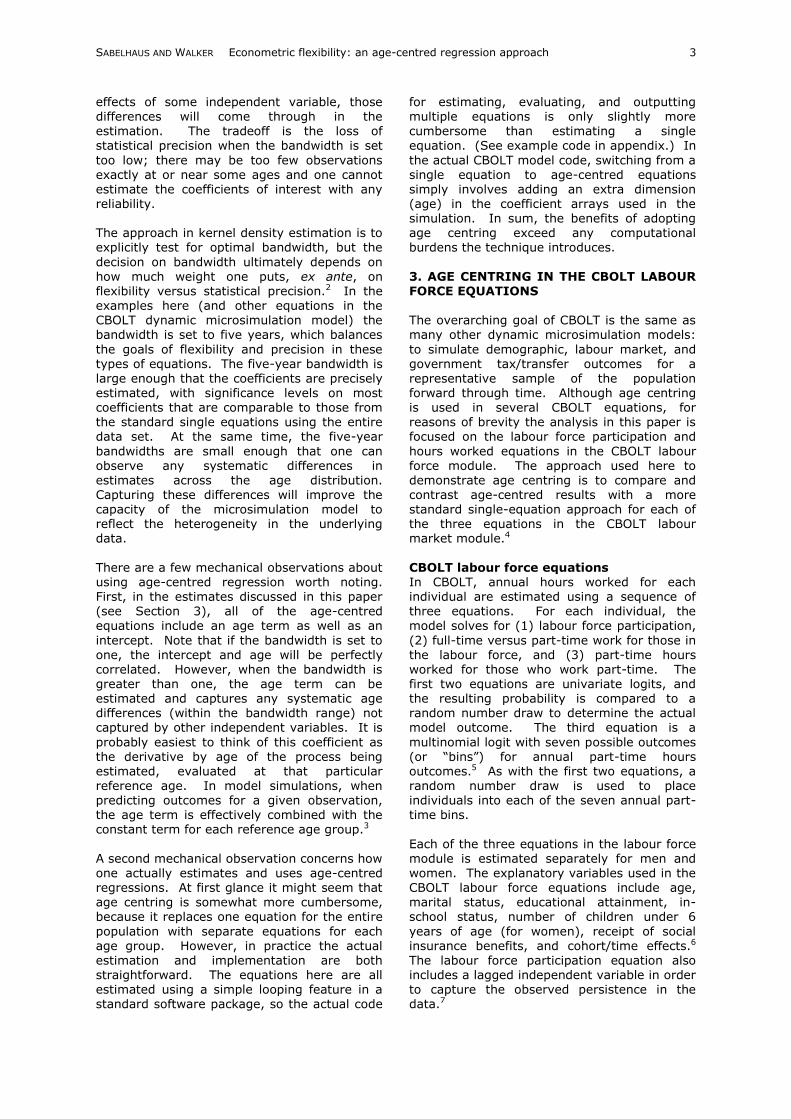
force participation noted above. Adding higher-order age terms to the equation may help the single-equation track better, but it is unlikely to eliminate the bias. Figure 4 shows the mean of part-time hours conditional on working part-time, and for these

outcomes the bias is even stronger. The effect


Figure 1 marginal effect of lagged LFP on labour force participation comparing single-equation and age-centred regressions men and women, ages 25-61

Figure 2 Marginal effect of being married on part-time hours worked comparing single-equation and age-centred regressions men and women, ages 25-61

of imposing a linear coefficient on age comes

through clearly for men, as the functional form induces a predicted relationship with age that is linear. As with labour force participation, the higher-order age-terms could improve predicted outcomes but the predictions will only asymptotically approach the age-centred

values as higher-order terms are added.

4. CONCLUSIONS

The technique described here as ―age-centred regression‖ analysis is a useful way to extract information from a limited data set when estimating equations for dynamic microsimulation models. The situation in

which age centring can help is very common:

0.5

0.55

0.6

0.65

0.7

0.75

0.8

0.85

0.9

25 26 27 28 29 30 31 32 33 34 35 36 37 38 39 40 41 42 43 44 45 46 47 48 49 50 51 52 53 54 55 56 57 58 59 60 61

Pro

po

rtio

n

Age

Women, Single-Equation

Men, Single-Equation

Women, Age-Centered

Men, Age-Centered

-150

-100

-50

0

50

100

150

25 26 27 28 29 30 31 32 33 34 35 36 37 38 39 40 41 42 43 44 45 46 47 48 49 50 51 52 53 54 55 56 57 58 59 60 61

Ho

urs

Wo

rked

Age



Women, Age-Centered

Men, Age-Centered


Figure 3 Mean predicted labour force participation comparing single-equation and age-centred

regressions men and women, ages 25-61

Figure 4 Mean expected part-time hours comparing single-equation and age-centred regressions

men and women, ages 25-61

when the behavioural process in question varies systematically by age and the effect of one or more independent variables might also

differ across age groups. The basic idea is to estimate separate equations for each age sample, but to include observations that are close to the reference age being estimated. Using the extra information from nearby observations makes it possible to statistically identify how marginal effects and predicted

mean outcomes differ across the age distribution under consideration.

The examples used here to illustrate age centring are fairly simple labour supply equations — the sequence of participation, full- versus part-time, and part-time hours given part- time employment — used in the Congressional Budget Office Long-Term (CBOLT) dynamic microsimulation. We show

0.4

0.5

0.6

0.7

0.8

0.9

1

25 26 27 28 29 30 31 32 33 34 35 36 37 38 39 40 41 42 43 44 45 46 47 48 49 50 51 52 53 54 55 56 57 58 59 60 61

Pro

po

rtio

n

Age

Men, Age-Centered

Women, Age-Centered



900

950

1000

1050

1100

1150

1200

25 26 27 28 29 30 31 32 33 34 35 36 37 38 39 40 41 42 43 44 45 46 47 48 49 50 51 52 53 54 55 56 57 58 59 60 61

Ho

urs

Age



Men, Age-Centered

Women, Age-Centered


that moving from a single-equation to an age-centred approach involves little loss of

statistical precision but has a significant impact on estimated marginal effects and mean

predicted outcomes by age. Acknowledgements The authors are grateful to the editor and an anonymous referee for suggestions. This paper was written while both authors were employed at the Congressional Budget Office,

Washington, DC. The analysis and conclusions in this paper are those of the authors and should not be interpreted as those of any of the institutions with which they have been affiliated over the course of this project.

Notes

1 Congressional Budget Office (2006). The

age-centring technique is also applied to marital transitions in CBO’s model; see O’Harra and Sabelhaus (2002) and Harris and O’Harra (2001). For a general overview of the CBOLT model see O’Harra, Sabelhaus, and Simpson (2004). The

model has been applied in several academic papers, such as Harris, Sabelhaus, and Simpson (2005), Harris and Sabelhaus (2005), Harris and Simpson (2005), and Sabelhaus and Topoleski (2007). There are also several published CBO reports and studies using CBOLT, available on the CBO

website under ―Publications by Study Area, Social Security and Pensions.‖

2 In particular, one is trading off the ability to

identify differences in the density at a particular point versus the precision with which that difference is being identified.

3 It is worth noting that this also can lead to a lot of apparent imprecision in the estimated constant and age terms, because if the slope of the process being estimated is relatively flat over a particular age range, there is too little variation by age to separately identify a constant and age

coefficient. Indeed, in some processes, one observes a pattern of estimated age and constant term coefficients that appear volatile, but the linear combination of the two actually input to the microsimulation model is much more stable.

4 For illustrative purposes we have chosen to

compare and contrast the age-centred equations with simple versions where age enters linearly, rather than equations with higher-order age terms, in order to emphasize the differences in properties. The primary difference we are trying to

highlight—the fact that coefficient estimates for independent variables other than age vary across age groups—is unaffected by

this decision. However, it is true that the mean predictions by age from the standard

model could be improved if we used higher-

order terms. 5 The bins for the multinomial logit are for

annual part-time hours of 125, 375, 625, 875, 1,125, 1,375, and 1,625. Everyone who works full-time (determined by the second equation in the module) has annual hours worked of 2,080.

6 Like most dynamic microsimulations, CBOLT does not attempt to explicitly incorporate structural equations such as in van Soest, Das, and Gong (2002). Therefore, the independent variable list does not include measures of wage or other labour income—

differences in earnings potential are captured by the education terms and in the idiosyncratic persistence term.

7 The other two equations—full-time versus part-time work, and part-time hours conditional on working part-time—exhibit the same longitudinal persistence as labour

force participation, but the CPS data used to estimate the equations do not have the requisite lagged information. CBOLT introduces that persistence into the simulation ex post using a technique described in Congressional Budget Office (2006).

8 CBOLT uses different equations and/or bandwidth limits for people under age 25 and over 61. For the young, the effects of schooling dominate labour force decisions. For people over 61 the effects of social insurance dominate labour force decisions,

because the eligibility age for Social Security is 62 in the United States.

9 Because the terminology is not universal, it is worth noting that ―Social Security‖ as described here includes only Old Age Survivors and Disability Insurance or OASDI, which covers standard worker

disability and retirement benefits. 10 This is not the only way to achieve desired

heterogeneity in labour market outcomes. For other examples, see the description of the labour force modules for the Urban Institute’s DYNASIM model in Favreault and Smith (2004) or for the Social Security

Administration’s Modeling Income in the Near Term (MINT) model in Toder et al. (2002).

11 The estimated thresholds or ―cut‖ para-meters are not shown for the part-time multinomial logits. Those are available

from the authors upon request. 12 The entire list of coefficients for reference

ages 16 through 70 can be found in Congressional Budget Office (2006).


REFERENCES

Congressional Budget Office (2006) ‘Projecting Labour Force Participation and Earnings in

CBO’s Long-Term Microsimulation Model’, Background Paper, Congressional Budget Office, Washington, DC.

Favreault M M and Smith K E (2004) ‘A Primer on the Dynamic Simulation of Income Model (DYNASIM3)’, Discussion Paper, Retirement Project, The Urban Institute, Washington,

DC. Harris A R and O’Harra J (2001) ‘The Impact of

Marriage and Labour Force Participation Trends on the Social Security Benefits of Women’, Proceedings of the National Tax Association, 99-107.

Harris A R, Sabelhaus J and Simpson M (2005) ‘Uncertainty About OAI Worker Benefits

Under Individual Accounts’, Contemporary Economic Policy, 23(1), 1-16.

Harris A R and Sabelhaus J (2005) ‘How Does Differential Mortality Affect Social Security Progressivity and Finances?’, Technical

Paper 2005-5, Congressional Budget Office, Washington, DC.

Harris A R and Simpson M (2005) ‘Winners and Losers Under Various Approaches to Slowing Social Security Benefit Growth’, National Tax Journal, LVIII(3), 523-544.

O’Harra J, Sabelhaus J and Simpson M (2004) ‘Overview of the Congressional Budget

Office Long-Term (CBOLT) Policy Simulation Model’, Technical Paper 2004-1, Congressional Budget Office, Washington DC.

O’Harra J and Sabelhaus J (2002) ‘Projecting Longitudinal Marriage Patterns for Long-Term Policy Analysis’, Technical Paper

2002-2, Congressional Budget Office, Washington, DC.

Sabelhaus J and Topoleski J (2007) ‘Uncertain Policy for an Uncertain World: The Case of Social Security’, Journal of Policy Analysis and Management, 26(3), 507-525.

Smith, K E, Cashin D B, and Favreault M M (2005) ‘Modeling Income in the Near Term

4’, The Urban Institute, Washington DC. Toder E, Thompson L H, Favreault M et al.

(2002) ‘Modeling Income in the Near Term: Revised Projections of Retirement Income Through 2020 for the 1931-1960 Birth

Cohorts’, The Urban Institute, Washington DC.

Van Soest A, Das M and Gong X (2002) ‘A Structural Labour Supply Model with Flexible Preferences’, Journal of Econometrics, 107(1-2), 345-374.

Appendix 1 Example implementation of age-centred regression in Stata The following is a generalised version of the Stata code used in the CBOLT model, provided

for demonstration purposes only. The full

version of the code takes account of sex and

age-specific differentials by implementing age-centred regression separately for a variety of

age group / sex combinations.

*Declare Stata version; clear any existing data, set memory size, turn off page pause version 6.0 clear set memory 500m

set more off *If files moved - change this directory reference AND the four data references below cd "C:\Labor Force and Earnings\LFP Equations\" * generate a log of Stata output log using LFP_modified_model,replace

*Declare lower bound age loop counters

local iage= 16 local jage=16 *Loop through all valid single years of age (90 = 90+ in this example)

* Note: 70+ group used in non age-centered regression estimate placed at end of example code while ìage'<=90 { *Call data file, deleting any existing data files use "C:\Labor Force and Earnings\lfp_master_file ", clear


*Set age-band (kernel) width to +/- 5 years from currently considered single year of age gen band=5

*Limit band-width if at or near top or bottom of age-range (= 16-90 in this example)

replace band=1 if ìage'==16|ìage'==90|ìage'>=61&ìage'<=66 replace band=2 if ìage'==17|ìage'==89|ìage'==60|ìage'==67 replace band=3 if ìage'==18|ìage'==88|ìage'==59|ìage'==68 replace band=4 if ìage'==19|ìage'==87|ìage'==58|ìage'==69 *Retain records (persons) in current analysis if age falls within range current age +/- band-width keep if age>=ìage'-band & age<=ìage'+band

*Declare a set of coefficients [default to 20], setting initial values to 0. gen beta1=0 gen beta2=0 gen beta3=0 gen beta4=0

gen beta5=0 gen beta6=0

gen beta7=0 gen beta8=0 gen beta9=0 gen beta10=0 gen beta11=0

gen beta12=0 gen beta13=0 gen beta14=0 gen beta15=0 gen beta16=0 gen beta17=0 gen beta18=0

gen beta19=0 gen beta20=0 *Assign weight for current record (person), based on difference from current loop single year of age

*[For 5-year age band, difference of 0 -> weight of 10; +/-1 -> 8; +/-2 -> 6; …etc.]

gen weight=(((band-abs(ìage'-age))/band)*10) * The following illustrative code provides an example of age-centred regression for age-band 16-18 only, * reflecting the common need to set up separate regressions for separate parts of the age range, in order * to capture changes in the key behavioural determinants. Hence the following code is executed

* conditional upon the current loop counter age value. while ìage'>16&ìage'<=18 { *Set cohort dummy variable to 1 if born during/after 1980 replace chort8=1 if birthyear>=1980

*Run logistic regression of Y [dep. varname] given X [indep. var names], in which the *variable pw (person weight] is set to equal calculated person-specific Kernel-density weight

logit lflwk lfp nm mar age in_school chort7 chort8 trend [pw=weight] *output stata-calculated predicted probability of labour force participation predict plfp, p

*tabulate output table age if age==ìage', c(mean plfp mean lflwk mean lfp) *keep 1st observation keep if _n==1


*Set value of beta coefficients equal to coefficients calculated by logistic regression

*replace betas that correspond to variables in the regression equation replace beta1=_b[age]

replace beta3=_b[_cons] replace beta10=_b[chort7] replace beta11=_b[chort8] replace beta12=_b[nm] replace beta13=_b[mar] replace beta14=_b[lfp] replace beta15=_b[trend]

replace beta16=_b[in_school] *Set string variable = current single year of age gen age_out=ìage' *Save results to age-specific file (concatenating generic file name with string variable recording

single *year of age), replacing any earlier version of file

save "C:\Labor Force and Earnings\lfp_ìage'", replace *Break out of loop, as each loop applies age-centred regression to one specific single year of age local iage=ìage'+100 }

*Update local age loop counters by 1 before going round loop again for next single year of age local iage=`jage'+1 local jage=`jage'+1 }

*For the final desired age-group (70+ in this example) conventional rather than age-centred regression is *used, therefore no weights are needed. However, everything else follows as in the above age-centred *example

clear use "C:\Labor Force and Earnings\lfp_master_file ", clear keep if age>=70 replace chort2=1 if birthyear>=1920 gen beta1=0 gen beta2=0 gen beta3=0

gen beta4=0 gen beta5=0 gen beta6=0 gen beta7=0 gen beta8=0 gen beta9=0 gen beta10=0

gen beta11=0 gen beta12=0

gen beta13=0 gen beta14=0 gen beta15=0 gen beta16=0

gen beta17=0 gen beta18=0 gen beta19=0 gen beta20=0 logit lflwk lfp nm mar age ssinc education2 education3 education4 chort1 chort2 trend predict plfp, p


table age if age>=70, c(mean plfp mean lflwk mean lfp) keep if _n==1

replace beta1=_b[age] replace beta2=_b[ssinc]

replace beta3=_b[_cons] replace beta4=_b[chort1] replace beta5=_b[chort2] replace beta12=_b[nm] replace beta13=_b[mar] replace beta14=_b[lfp] replace beta15=_b[trend]

replace beta17=_b[education2] replace beta18=_b[education3] replace beta19=_b[education4] gen age_out=70 save "C:\Labor Force and Earnings\lfp_70", replace

use "C:\Shared\Labor Force and Earnings\lfp_16", clear local iage=17

while ìage'<=70 { append using "C:\Labor Force and Earnings\lfp_ìage'" local iage=ìage'+1 }

*Write out age-centred regression coefficients and save to file [lfp_modified_model] outfile age_out beta1 beta2 beta3 beta4 beta5 beta6 beta7 /* */ beta8 beta9 beta10 beta11 beta12 beta13 beta14 beta15 /* */ beta16 beta17 beta18 beta19 beta20 /* */ using C:\Labor Force and Earnings\lfp_modified_model.txt, wide replace

Documents

ECONOMETRIC FLEXIBILITY IN … FLEXIBILITY IN MICROSIMULATION: AN AGE-CENTRED REGRESSION ... available data set for estimating a model equation is ... the single equation approach