ECON4510 Finance Theory Lecture 12 - UiO

ECON4510 – Finance TheoryLecture 12

Kjetil StoreslettenDepartment of Economics

University of Oslo

April 26, 2018

Kjetil Storesletten, Dept. of Economics, UiO ECON4510 Lecture 10 April 26, 2018 1 / 24

Valuation of options before expiration

Need to distinguish between American and European options.

Consider European options with time t until expiration.

Value now of receiving cT at expiration? (Later also pT .)

Have candidate model already: Use CAPM?

Problematic: Non-linear functions of ST .

Difficult to calculate E (cT ) and cov(cT , rM).

Instead: Theory especially developed for options.

(But turns out to have other applications as well.)

“Valuation of derivative assets.”

Value of one asset as function of value of another.

Will find c(S , . . .) and p(S , . . .).

Other variables (—hopefully observable—) as arguments besides S .


Net value diagrams (Hull 9th, figs. 10.1–10.4, 12.1–12.12)

(8th ed. figs. 9.1–9.4, 11.1–11.12, 7th ed. 8.1–8.4, 10.1–10.12)

Value at expiration minus purchase cost.

ST on horizontal axsis. (Some examples, blackboard)

Fig. 10.1: cT − c , buying a call option.

Resembles gross value, cT , diagram.

But removed vertically by subtracting c , today’s price.

These diagrams only approximately true:I No present-value correction for time lag −c to cT .I There isn’t one exact relationship between c and cT .

F That exact relationship depends on other variables.

Fig. 10.3: c − cT , selling a call option.

Observe: Selling and buying cancel out for each ST .

Options redistribute risks (only). Zero-sum.


Net value diagrams, contd.

Similar to fig. 12.10: Buy share, buy two put options with S = K .

(Hull uses another combination to get the same effect in fig. 12.10.)

Diagrams show ST − S , 2pT − 2p, ST − S + 2pT − 2p.

Good idea if you believe ST will be different from S (and K ), but youdo not know direction.

Fig. 12.1(c): Buy put option with K = S , plus one share.

pT − p + ST − S .

Resembles value of call option.

Will soon show exact relationship to call option.


Determinants of option value (informally)

Six candidates for explanatory variables for c and p:

S , today’s share price. Higher S means market expects higher ST ,implies higher c (because higher cT ), lower p (lower pT ).

K , the striking price. Higher K means lower c (because lower cT ),higher p (higher pT ).

Uncertainty. Higher uncertainty implies both higher c and higher p,because option owner gains from extreme outcomes in one direction,while being protected in opposite direction. (Remark: This is totalrisk in ST , not β from CAPM.)


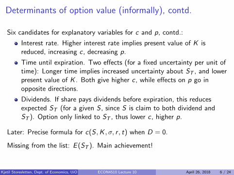
Determinants of option value (informally), contd.

Six candidates for explanatory variables for c and p, contd.:

Interest rate. Higher interest rate implies present value of K isreduced, increasing c , decreasing p.

Time until expiration. Two effects (for a fixed uncertainty per unit oftime): Longer time implies increased uncertainty about ST , and lowerpresent value of K . Both give higher c, while effects on p go inopposite directions.

Dividends. If share pays dividends before expiration, this reducesexpected ST (for a given S , since S is claim to both dividend andST ). Option only linked to ST , thus lower c , higher p.

Later: Precise formula for c(S ,K , σ, r , t) when D = 0.

Missing from the list: E (ST ). Main achievement!


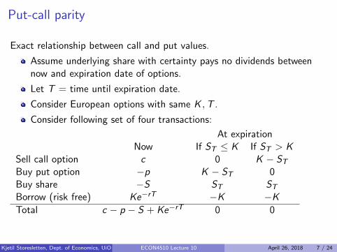
Put-call parity

Exact relationship between call and put values.

Assume underlying share with certainty pays no dividends betweennow and expiration date of options.

Let T = time until expiration date.

Consider European options with same K ,T .

Consider following set of four transactions:

At expirationNow If ST ≤ K If ST > K

Sell call option c 0 K − STBuy put option −p K − ST 0Buy share −S ST STBorrow (risk free) Ke−rT −K −KTotal c − p − S + Ke−rT 0 0


Put-call parity, contd.

Must have c = p + S − Ke−rT , if not, riskless arbitrage.

To exploit arbitrage if, e.g., c > p + S − Ke−rT :

“Buy cheaper, sell more expensive.”

Sell (i.e., write) call option.

Buy put option and share.

Borrow Ke−rT .

Receive c − p − S + Ke−rT > 0 now.

At expiration: Net outlay zero whatever ST is.

Put-call parity allows us to concentrate on (e.g.) calls.


Allow for uncertain dividends

Share may pay dividends before expiration of option.

These drain share value, do not accrue to call option.

In Norway dividends paid once a year, in U.S., typically 4 times.

Only short periods without dividends.

Theoretically easily handled if dividends are known.

But in practice: Not known with certainty.

For short periods: S ≈ E (D + ST ).

For given S , a higher D means lower ST , lower c , higher p.

Intuitive: High D means less left in corporation, thus option to buyshare at K is less valuable.

Intuitive: High D means less left in corporation, thus option to sellshare at K is more valuable.


Allow for uncertain dividends, contd.

Absence-of-arbitrage proofs rely on short sales.

Short sale of shares: Must compensate for dividends.

Short sale starts with borrowing share. Must compensate the lenderof the share for the dividends missing. (Cannot just hand back sharelater, neglecting dividends in meantime.)

When a-o-arbitrage proof involves shares: Could in some casesassume D = 0 with full certainty.

If not D = 0 with certainty, conclude with inequalities instead ofequalities.


More inequality results on option values

Absence-of-arbitrage proofs for American calls:

1 C ≥ 0: If not, buy option, keep until expiration. Get somethingpositive now, certainly nothing negative later.

2 C ≤ S : If not, buy share, sell (i.e., write) call, receive C − S > 0. GetK > 0 if option is exercised, get S if not.

3 C ≥ S − K : If not, buy option, exercise immediately.

4 When (for sure) no dividends: C ≥ S − Ke−rT : If not, do thefollowing:

ExpirationNow Div. date If ST ≤ K If ST > K

Sell share S 0 −ST −STBuy call −C 0 0 ST − KLend −Ke−rT 0 K K

> 0 0 ≥ 0 0

A riskless arbitrage.


More inequality results on option values

Important implication: American call option on shares which certainly willnot pay dividends before option’s expiration, should not be exercisedbefore expiration, since

C ≥ S − Ke−rT > S − K .

Worth more “alive than dead.” When no dividends: Value of Americancall equal to value of European, since it is not rational to exercise theseoptions early.


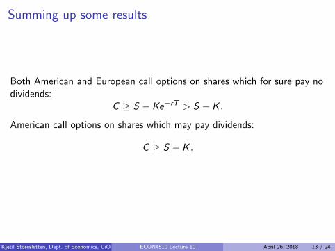
Summing up some results

Both American and European call options on shares which for sure pay nodividends:

C ≥ S − Ke−rT > S − K .

American call options on shares which may pay dividends:

C ≥ S − K .


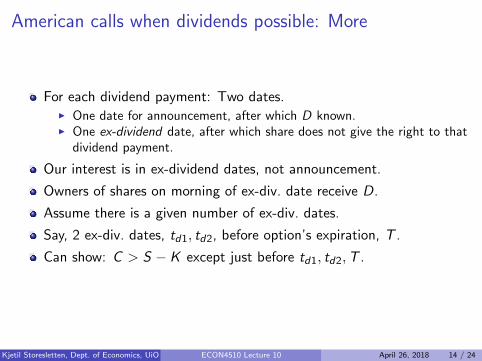
American calls when dividends possible: More

For each dividend payment: Two dates.I One date for announcement, after which D known.I One ex-dividend date, after which share does not give the right to that

dividend payment.

Our interest is in ex-dividend dates, not announcement.

Owners of shares on morning of ex-div. date receive D.

Assume there is a given number of ex-div. dates.

Say, 2 ex-div. dates, td1, td2, before option’s expiration, T .

Can show: C > S − K except just before td1, td2,T .


American calls when dividends possible: More

Assume contrary, C ≤ S − K . Then riskless arbitrage:

Buy call, exercise just before:Now Just before next tdi or T

Buy call −C S − KSell share S −SLend −K Ker∆t

≥ 0 K (er∆t − 1)

Riskless arbitrage, except if ∆t ≈ 0, just before.

Implication: When possible ex-dividend dates are known, American calloptions should never be exercised except perhaps just before one of these,or at expiration.


Trading strategies with options, Hull 9th ed., ch. 12

(8th ed., ch. 11, 7th ed., ch. 10)

Consider profits as functions of ST .

Can obtain different patterns by combining different options.

Example: bear spread, Hull fig. 12.5

Strategies in ch. 12 sorted like this:I Sect. 12.1: One option, one share.I Sect. 12.2: 2 or 3 calls, or 2 or 3 puts, different K values.I End of 12.3, pp. 265–266:1 Different expiration dates.I Sect. 12.3: “Combinations”, involving both puts and calls.

Among these types of strategies, those with different expiration datescannot be described by same method as others.

18th ed., pp. 244–245, 7th ed., pp. 227–229Kjetil Storesletten, Dept. of Economics, UiO ECON4510 Lecture 10 April 26, 2018 16 / 24

Trading strategies with options, Hull 9th ed., ch. 12

(8th ed., ch. 11, 7th ed., ch. 10)

The first, second, and fourth type:I Use diagram for values at expiration for each security involved.I Payoff at expiration is found by adding and subtracting these values.I Net profit is found by subtracting initial outlay from payoff.I Initial outlay could be negative (if, e.g., short sale of share).I Remember: No exact relationship between payoff and initial outlay is

used in these diagrams — will depend upon, e.g., time until expiration,volatility, interest rate.

For the third type: “Profit diagrams for calendar spreads are usuallyproduced so that they show the profit when the short-maturity optionexpires on the assumption that the long-maturity option is closed outat that time” (Hull 9th ed., p. 265).2

28th ed., p. 244, 7th ed., p. 228Kjetil Storesletten, Dept. of Economics, UiO ECON4510 Lecture 10 April 26, 2018 17 / 24

Developing an exact option pricing formula

Exact formula based on observables very useful.

Most used: Black and Scholes formula.

Fischer Black and Myron Scholes, 1973.

Their original derivation used difficult math.

Continuous-time stochastic processes.

First here: (Pedagogical tool:) Discrete time.

Assume trade takes place, e.g., once per week.

Option pricing formula in discrete time model.

Then let time interval length decrease.

Limit as interval length goes to zero.

Option pricing formula in continuous time.


Common assumptions

1 No riskless arbitrage exists.

2 Short sales are allowed.

3 No taxes or transaction costs.

4 Exists a constant risk free interest rate, r .

5 Trade takes place at each available point in time. (Two differentinterpretations: Once per period, or continuously.)

6 St+s/St is stochastically independent of St and history before t.


Separate assumptions (discrete = d, continuous = c)

7d. St+1/St has two possibleoutcomes, u and d . Ev-eryone agrees on these.

7c. Any sample path {St}Tt=0

is continuous.

8d. Pr(St+1/St = u) = p∗

for all t.8c. var[ln(St+s/St)] = σ2s.

Everyone agrees on this.

9d. St+s has a binomial dis-tribution.

9c. St+s has a lognormal dis-tribution.


Discrete time binomial share price process

��

XXXXX

��

XXXXX

��

XXXXX

��

XXXXX

��

XXXXX

��

XXXXX

u · S0

d · S0

u2 · S0

du · S0

d2 · S0

d3 · S0

d2u · S0

du2 · S0

u3 · S0

S0


Discrete time binomial share price process

Define Xn = St+n/St . (These are stochastic variables as viewed from timet. Their distributions do not depend on t.)

Pr(X1 = u) = p∗.

For this course we will not go into detail on the following:

Pr(Xn = ujdn−j) =n!

j!(n − j)!p∗j(1− p∗)n−j ,

the binomial probability for exactly j outcomes of one type (here u) withprobability p∗, in n independent draws. (j ≤ n.)

Pr(Xn ≥ uadn−a) =n∑

j=a

n!

j!(n − j)!p∗j(1− p∗)n−j


Corresponding trees for share and option

��

��

XXXXXXXXXX

p∗

1− p∗

u · S

d · S

S

��

��

XXXXXXXXXX

p∗

1− p∗

cu = max(0, uS − K )

cd = max(0, dS − K )

c


Corresponding trees for share and option

Value of call option with expiration one period ahead?

“Corresponding trees” mean that option value has upper outcome ifand only if share value has upper outcome.

For any K , know the two possible outcomes for c .

I.e., for a particular option, cu, cd known.

If K ≤ dS , then cd = dS − K , cu = uS − K .

If dS < K ≤ uS , then cd = 0, cu = uS − K .

If uS < K , then cd = 0, cu = 0.

This third kind of option is obviously worthless.


Documents

ECON4510 Finance Theory Lecture 12 - UiO