ECON3300.2 INTERMEDIATE MICROECONOMICS-Winter 2012foroughfarrokhzad.tripod.com/.../econ3300_winter2012.pdf · The economy is a complex system made of the interaction of individual

Saint Mary’s University- Sobey School of Business

Page 1 of 2

ECON3300.2 INTERMEDIATE MICROECONOMICS-Winter 2012 Dr. Maryam Dilmaghani Office: 348 Sobey Building Phone: (902) 420-6242 Email: [email protected] Webpage: http://www.neuropsyconomics.com/

Lecture Time: Monday & Wednesday, 2:30 pm - 3:45 pm

Lecture Time and Location

Lecture Location: Burke Building 218

Tuesdays: 2:00 p.m. to 6:00 p.m.

Office Hours

In case you cannot make the designated hours email me for an appointment.

Emailed questions will be answered within reasonable delay.

ECON1201 (Microeconomics) and ECON1202 (Macroeconomics) or special authorization from the department.

Course Prerequisites

The economy is a complex system made of the interaction of individual decision makers. Therefore, precision of language is necessary to the comprehension of economic relationships. This course is designed to present a logical and coherent framework in which to organize observed economic phenomena. Microeconomic theory is based on the notion that individuals (and firms) have well defined objectives (e.g., maximizing satisfaction or profits) and behave systematically according to the incentives and constraints of their economic environment.

Course Description

Upon completing this course you should be able to understand and provide illustrations of the role of markets in allocating scarce resources, the impact of government intervention in the market and the debates relating social welfare, involving business and politics.

References and Textbooks

Intermediate Microeconomics A Modern Approach, Hal Varian, WW Norton, the latest edition. Some additional reading might be assigned during the course and posted in Blackboard.

mailto:[email protected]�

http://www.neuropsyconomics.com/�

Saint Mary’s University- Sobey School of Business

Page 2 of 2

1.

Grading Scheme

Four Assignments, each accounting for 5% of final grade 20%

2. Midterm (70 minutes, February 13th: tentative) 30%

3. Final Examination 50%

4. Bonus points from in-class popup quizzes 5%

The assignments will be distributed in class and are due one week after the date of circulation. The midterm will be held during regular class hours on the date given below. It is your responsibility to appear for all exams as scheduled.

Policies Related to Assignment and Exams

If the midterm examination is missed and the absence is justified its weight will be transferred to final exam. In such cases the students are encouraged to get in touch with me as soon as possible.

Periodically, students will be given an in-class quiz drawing upon the same day’s lectures. The quizzes will be marked and returned and participant may gain up to 5% bonus points through their performance in this quizzes. The intention is to encourage the students to focus on and follow the lecture.

Students will abide by Saint Mary’s regulations concerning academic integrity.

Important Note

For more information see:

http://www.smu.ca/registrar/documents/Undergraduate20112012.pdf

Calculators and Dictionaries

The calculators are allowed during exams, but only non-programmable ones. Programmable or financial calculators are not allowed. The use of paper dictionaries during the exam is also allowed.

The deadline to drop this course is March 16th 2012 (University’s End of withdrawal period for fall-term 3 credit courses). Students who have special needs or any specific condition are encouraged to speak with me as soon as possible.

Miscellaneous

http://www.smu.ca/registrar/documents/Undergraduate20112012.pdf�

Saint Mary’s University-Sobey School of Business

Welcome to all!

1

Prepared by Dr. Maryam Dilmaghani

Winter 2012

Adam Smith

ECON3300.: Intermediate Microeconomics

ECON3300.: Intermediate Microeconomics 2

Happy New Year!

Adam Smith

3

Adam Smith (1723 –1790) was a Scottish moral philosopher and a pioneer of political economics.

One of the key figures of the Scottish Enlightenment, Smith is the author of The Theory of Moral Sentiments and An Inquiry into the Nature and Causes of the Wealth of Nations.

The Wealth of Nations, is considered his magnum opus and the first modern work of economics. Smith is widely cited as the father of modern economics.


ECON3300: Intermediate Microeconomics

4

The objective of this course is to introduce students to a more in -depth and technical level of understanding microeconomics.

The course focuses on the study of the economic behaviour of individual households (consumers) and firms (producers).

It then gets to the study of markets and the determination of the market prices of individual goods and services under different market structures.


Instructor

5

Dr. Maryam Dilmaghani Office: 348 Sobey Building

Phone: (902) 420-6242 Email: [email protected] Webpage: http://www.neuropsyconomics.com/

Office Hours Tuesdays: 2:00 p.m. to 6:00 p.m. In case you cannot make the designated hours email me for an

appointment.


mailto:[email protected]�

http://www.neuropsyconomics.com/�

Textbook


Required : Intermediate Microeconomics A Modern

Approach, Hal Varian, WW Norton, the latest edition. Some additional reading might be assigned during the course and posted in Blackboard.

Additional readings and handouts will be assigned and posted in Blackboard.

Grading Scheme

7

1. Two Assignments 20%

2. Midterm (70 minutes, Feb. 13th : tentative) 30%

3. Final Examination 50%

4. Bonus points from in-class popup quizzes Up to 5%


Facebook Page


Facebook news feed for this course: https://www.facebook.com/smueconcourses

The news articles related to this course or other on-line texts and

materials will be posted in this page along a short commentary or discussion question.

The topics covered in this course will allow the students to effectively follow such news article by the end of the term.

https://www.facebook.com/smueconcourses�

Practical Advice

9

Attending the lectures helps knowing important points and possible misunderstandings that may arise when you do the readings.

Many problem sets will be provided and exams will draw upon them. Practicing them is a key to a good grade.

Come to my office hours and ask your questions regularly: the topics in this course build upon each other, hence, falling behind can have undesirable consequences.

Please share your suggestions with me.



Just Warm-up!

11

What is Education?


What is Education...

Albert Einstein: “Education is what remains after one has forgotten everything

he learned in school.”

12

Einstein on his 72nd birthday , 1951


13

What is Teaching?


What is Teaching...

Albert Einstein: “Teaching should be such that what is offered is perceived as

a valuable gift and not as a hard duty.” “I never teach my pupils; I only attempt to provide the

conditions in which they can learn.”

14 ECON3300.: Intermediate Microeconomics

15

What is Understanding?


What is Understanding...

16

Albert Einstein: “You do not really understand something unless you can

explain it to your grandmother.”


Questioning...

17

Albert Einstein: “The important thing is not to stop questioning. Curiosity has

its own reason for existing.”


Value of Science...

18

Albert Einstein: “One thing I have learned in a long life: that all our science,

measured against reality, is primitive and childlike and yet it is the most precious thing we have.”


Practical Advice

19

Attending the lectures helps knowing important points and possible misunderstandings that may arise when you do the readings.

Many problem sets will be provided and exams will draw upon them. Practicing them is a key to a good grade.

Come to my office hours and ask your questions regularly.

Please share your suggestions with me.


List of Topics

20

Introduction to Concepts & Techniques Consumer Behaviour

Producer Behaviour

Markets

Market Structure

Others


21

What is Education?


What is Education...

Albert Einstein: “Education is what remains after one has forgotten everything

he learned in school.”

22

Einstein on his 72nd birthday , 1951


23

What is Teaching?


What is Teaching...

Albert Einstein: “Teaching should be such that what is offered is perceived as

a valuable gift and not as a hard duty.” “I never teach my pupils; I only attempt to provide the

conditions in which they can learn.”

24 ECON3300.: Intermediate Microeconomics

25

What is Understanding?


What is Understanding...

26

Albert Einstein: “You do not really understand something unless you can

explain it to your grandmother.”


Questioning...

27

Albert Einstein: “The important thing is not to stop questioning. Curiosity has

its own reason for existing.”


Value of Science...

28

Albert Einstein: “One thing I have learned in a long life: that all our science,

measured against reality, is primitive and childlike and yet it is the most precious thing we have.”



Just Warm-up!

30

What is complexity in a system?


31

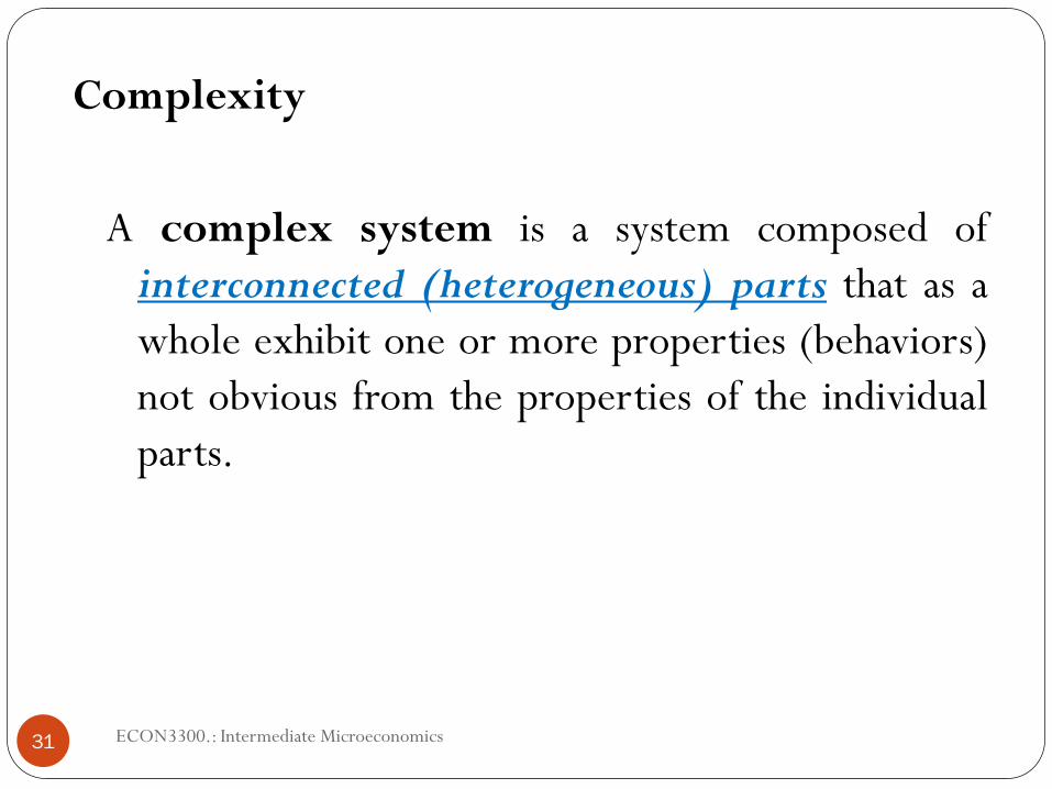
A complex system is a system composed of interconnected (heterogeneous) parts that as a whole exhibit one or more properties (behaviors) not obvious from the properties of the individual parts.

Complexity


32

What is self-organisation in a system?


Self-Organisation

33

Self-organization is the process where a structure or pattern appears in a system without a central authority or external element imposing it through planning.


Complexity & Self-Organization

34

Implications for Economy and Economics

Hard to predict the future state o the system

Intervention may lead to unexpected changes in the outcomes (previous patterns)


Market Economy…

35

As a complex system.

Why and How?

As a self-organized system.

Why and How?


Market Economy and Economics

36

Adam Smith: The Discovery of Invisible Hand

Invisible Hand is said to work to achieve collective good without having any prior intention for this end (collective good) behind.

How Does Invisible Hand Work?


Economic Agents

37

What are the properties of economic agents (people who are forming human societies)?

Self-interest

Rationality

Amounting to responding to incentives that are set through market indicators (price system) and institutions.


Alternative to Market Economy

38

Karl Marx and Trying to Outperform Invisible Hand by Central Planning.

Experience and history shows very limited success, the reason is a combination of many factors (e.g. the nature of human incentives).

Karl Marx (1818 –1883), German

philosopher, political economist, political theorist, communist.


39

What is Scarcity?

What is the implication of Scarcity?


Opportunity Cost

40

Opportunity cost is the worth of the next-best available choice which is forgone in order to have the current choice.

Opportunity cost is expressing the basic relationship between scarcity and choice.

The concept of an opportunity cost was first developed by John Stuart Mill.

John Stuart Mill (1806 -1873)


http://upload.wikimedia.org/wikipedia/commons/4/43/John_Stuart_Mill_by_John_Watkins,_1865.jpg�

Economic Methodology

41

Using Figures to convey Information

Using Charts and Tables to convey Information

Using Models and Equations to convey Information


Representing scarcity...

42

Suppose Alice has $24.

She is thinking of spending it on Bottles of Beer and/or Slices of Pizza.

The price of a slice of pizza is $2 and the price of a bottle of beer is $3.

Let us represent Alice possibilities in a Figure...


Opportunity Cost and “Possibilities”

43

Pizza (QP)

Beer (QB )

8

12 Possible Combinations

Boundary

- Pizza

+Beer

Unattainable Combinations


44

Now let us represent Alice possibilities by an Equation...


ECON3300 Winter 2012 SMU-Sobey SB

Page 1 of 5

Intermediate Microeconomics Instructor: Dr. Maryam, Dilmaghani

Utility Function

In economics, utility is a measure of relative satisfaction from quantity consumed of goods or

services (also from the possession of wealth and spending of leisure time).

Utility is assumed to be:

(i) a function of quantity consumed (see below: Quantity consumed is on the x-axis and Utility of the total quantity consumed is on the y-axis)

(ii) Increasing with decreasing rate (see the shape of the figure below).

Quantity

Utility


Page 2 of 5

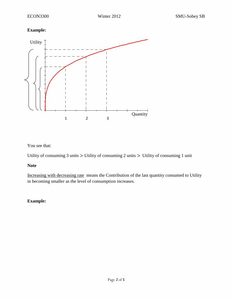
Example:

You see that:

Utility of consuming 3 units > Utility of consuming 2 units > Utility of consuming 1 unit

Note

Increasing with decreasing rate

means the Contribution of the last quantity consumed to Utility in becoming smaller as the level of consumption increases.

Example:

Quantity

Utility

1 2 3


Page 3 of 5

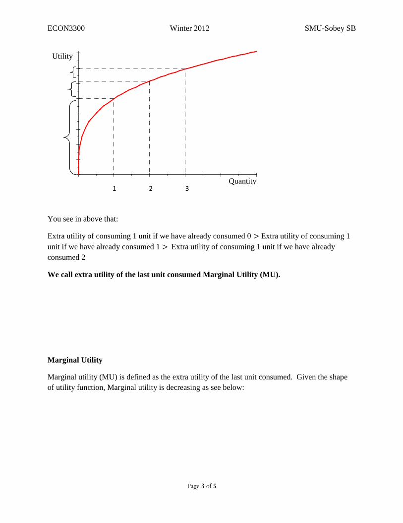
You see in above that:

Extra utility of consuming 1 unit if we have already consumed 0 > Extra utility of consuming 1 unit if we have already consumed 1 > Extra utility of consuming 1 unit if we have already consumed 2

We call extra utility of the last unit consumed Marginal Utility (MU).

Marginal Utility

Marginal utility (MU) is defined as the extra utility of the last unit consumed. Given the shape of utility function, Marginal utility is decreasing as see below:

Quantity

Utility

1 2 3


Page 4 of 5

Example:

Utility function can help representing a consumer satisfaction and also in combination with prices and income, representing the demand curve.

Short Answer Questions

Quantity

MU

Quantity

MU

1 2 3


Page 5 of 5

1. What is utility function? Illustrate.

2. What is marginal utility? Illustrate.

3. If consumption increases from 4 units to 5 units then utility falls: True/False? Why?

4. If consumption increases from 4 units to 5 units then marginal utility falls: True/False? Why?

5. Utility function provides enough information to find the demand curve: True/False? Why?


Page 1 of 2

Optional Review of Production Function (Principles of Micro). Recommended.

Production

Instructor: Dr. Maryam Dilmaghani

Hhh

0

200

400

600

800

1000

1200

1400

1 2 3 4 5 6 7 8 9 10 11 12 13 14 15 16 17 18

TP


Page 2 of 2

-40

-20

0

20

40

60

80

100

120

1 2 3 4 5 6 7 8 9 10 11 12 13 14 15 16 17 18

AP MP


Page 1 of 4

Optional Review of Production Function (Principles of Micro). Recommended.

A. Production in short-run


1. Total Product

The production function, relating the quantity of the variable input (labour) to the total quantity produced, below is assumed because its features are sensible. They are:

(i) Total product is increasing with an increasing rate: Marginal Product increasing

(ii) Total product is increasing with a decreasing rate: Marginal Product decreasing

(iii) Above certain level of total output (production plant’s capacity) total product decreases if we increase the quantity of input.

0 20 40 60 80 100 120 140 160 1800

10000

20000

30000

40000

50000

60000

L

Q

MP is increasing MP is decreasing MP is negative

Maximum Total Product


Page 2 of 4

2. Marginal (Red) and Average (Green) Product

(i) At the beginning, MP is higher than AP. It is so because MP is increasing.

(ii) Then although MP starts to fall, AP remains increasing with quantity f input (labour). It is so because low level of productivity at the beginning of production process.

(iii) As soon is MP is smaller than AP (below, as you see in the curves), MP should start falling. It means that MP intersects with AP at its maximum.

20 40 60 80 100 120 140 160 180 2000

100

200

300

400

500

L

Q

MP is increasing MP is increasing

Maximum Average Product


Page 3 of 4

B. Marginal (Red) and Average (Blue) Functions

Note: Cost functions are specified as a function of quantity produced (output), as opposed to quantity of input. However how output produced related to the quantity of input employed impacts the shape of cost functions.

(i) Marginal cost falls as at the beginning of the production process MP is increasing. It means that contribution of every unit of input hired in to total output is becoming larger and larger.

Given that, per unit cost of input remains the same marginal cost falls. For the same reason average cost falls as well.

(ii) As MP starts falling, Mc starts rising. However, AC still keep falling for a whole given the high MCs (low MP) at the beginning of the production process.

200 300 400 500 600 700 800 9000

1e+5

2e+5

3e+5

Q

$

Minimum Average Product

Marginal Cost Increasing Marginal Cost Decreasing


Page 4 of 4

(iii) As soon as MC is higher than average cost (is above as you see in the figure), AC starts rising.

Intermediate Microeconomics, Crash Review

SMU-ECON3300 Winter 2012

1

David Ricardo (1772-1823) English Political Economist

©Prepared by Dr. Maryam Dilmaghani ECON3300- Winter 2012

About these Slides

2

I have prepared these slide sets to include the main elements of Consumer and Producer Theory that we have covered so far.

Note that the slides are summaries and do not provide preparation for solving questions.

The must be used as a complement to the notes and problem sets and the book and means of quick review and check if the important concepts are learned.

MD

ECON3300- Winter 2012

Economic Model

3

In economic theory we often talk about Models.

A model is an abstract construct that represents a given economic situation through the use of variables and logical relationships between them.

Logical relationship between variables are derived from a set of principles (axioms of choice, arithmetic etc.)

A model is developed to address a specific issue (and not the possibilities outside it).

A model is a useful tool in that it can provide predictions about the outcome of a real world situation. A model may also help understanding a real world outcome.


Decision making

4

Economic agents are characterized by making rational decisions with respect to their economic affairs. Rational decision practically means it follows an objective and it is consistent with the best ways of achieving this objective.

Concretely individual agents are believed to be making rational decisions if they maximize their utility (and that leads to demand function) and firms to maximize their profits (and that leads to supply function).

Economic profit is different from what it means in everyday language by being defined as the divergence between benefits and costs where costs are inclusive of all compensations. Utility is a metaphor for units of satisfaction and in the most economic contexts the satisfaction comes from consumption.


Price : Invisible Hand’s Fingerprint A numerical value that indicates the economy’s consensus about the relative

worth of the goods (and services). An exchange ratio between goods traded for each other.

Price is based on relative scarcity (in its economic sense) of goods and services.

In economic models can talk about price as a magnitude only when Money is formally introduced. It will not be the case in this course: that is why we should talk about relative price.

Price is an endogenous variable which means it is determined by the “factual relative scarcity” of goods and services that it helps being exchanged. Economic scarcity of goods is a function of both availability (supply) and desirability (demand).

5 ECON3300- Winter 2012

Market Market in economic terms is not a physical place but a concept: The set of units (producers/sellers and consumers/buyers) that are

involved in the exchange of a given product requiring the simultaneous presence of supply and demand.

A virtual place in which apple is traded against another valued object (inclusive of money) constitutes the Market for Apple.

“A market ” may be equivalent to “A Sector” or “An Industry”

in this course.

Essential of market: presence of sellers and buyers of a none-free product whose value is possible to measure.


Efficiency: it is a Principle Efficiency in Production is:

Using available resources in a way to maximize the production of goods and services or When no more output can be obtained without increasing the amount of inputs or when production proceeds at the lowest possible per-unit cost. How?

Efficiency in Consumption means: Utility (satisfaction) cannot be increase through any other reallocation

of available resources (consumers’ budget constraint). How?


Resource constraints Note that economics would not exist if we did not face

(economics) resource constraints. Resource constraint means that inputs to production (and

budget) are not infinite but are available at a limited amount.

The job of economist is to plan to use no more and no less than the available resource:

Using more than available resources is impossible and using less than available resources is not optimal (we will soon see what optimal means).


Market Equilibrium A state of the world where economic forces are balanced and in the

absence of external influences the values of economic variables will not change. A simple characterization of market equilibrium is the price and quantity at which demand and supply coincide.

An equilibrium with flexible price is referred to as Competitive Equilibrium.

An inter-related multi-market equilibrium is referred to as General Equilibrium.

Market equilibrium carries no normative meaning or positive value judgment: markets may be in equilibrium at the same time that people are starving.


Market Mechanism

10

Market is conceptualized through supply and demand function (of price). If at a given price supply and demand are not equal then the market is not at equilibrium : there is either Execs Supply or Excess Demand.

Execs Supply and Excess Demand are the forces that help the re-establishment of market equilibrium (through price adjustment):

Excess Demand pushes the price upward (remember: price is a function of economic scarcity) and as the price goes up quantity supplied increases as well until new equilibrium emerges. (And excess supply is…)


A Market and its equilibrium: an illustration

11

Suppose for any given price quantity demanded increases (Demand curve shift rightward).

S

D2

Exces D.

Quantity

D1

Price

Demand shift

Q1 Q2

P1

P2


General Equilibrium

12

Understanding international trade involves understanding the reasons behind and the implications of the movement of goods produced in one country to the other.

Providing any sensible explanation for such processes generally involves talking about several interrelated markets (various inputs and various outputs).

That is why most international trade models are set in General equilibrium (GE) setting: it means we consider impacts of interrelation between markets (production and consumption).


Supply and Demand

Demand describes the consumer side of market.

Demand is an indicator of desirability hence or the benefit of a good.

Supply and demand is an indicator of availability or economic cost of a good.

Now we will see where Supply and Demand come from. 13 ECON3300- Winter 2012

Indifference Curves (IC)

14

Apple

Banana

IC

An Indifference curve represents various combinations of two products that yield the same level of satisfaction. Higher consumption of both good means higher level of satisfaction.

Higher satisfaction


Choice

15

Apple

Banana

BC

Budget Constraint and IC lead to choice. BC is various combination of goods that you can have given the resource you dispose and the prices.


Demand-1

16

Deamnd curve represents the quantity ‘a person’ is ready to buy at a given price. It is downward sloping.

D P

Q


Demand-2

17

Demand curves shifts if taste or income changes.

The slope of the curve shows the price sensitivity of the demand. The higher the slope the lower the sensitivity.

Q

P P

D1

D2

∆Q1 ∆Q2


Consumer Surplus

D

P1

P2


Production A production function describes the quantity of output that can be

produced using a set of inputs and technology.

Usually more inputs mean more output but sensitivity of the level of output to employed inputs differs.

An input can be required at a fixed amount at the scale of a firm (fixed input) or a function of quantity of output (variable input).


Production Function

K

Suppose K is capital invested and Y is output.

Y

Production-1

Production-2


Marginal Product

MPK

MPK

21

K1 K2

The incremental change in output arising from the use of one additional unit of the variable input. Usually it is assumed to be declining.

MPK1

MPK2


Economic Costs Cost is a measure of the alternative use that the employed resources

could have (in the present and/or in the future) compared to their actual use. It can be measured in monetary or real terms.

Costs can be viewed

Privately: costs to individuals or firms

Socially: costs to present and/or future society

Opportunity Cost (OC) is the value of an alternative that one forgoes in order to have the other. By default we talk about OC in per unit terms.


Production Costs

23

Several measures exist for production costs: Total Cost (TC) = Cost (price) of all inputs used to produce the output.

Fixed Costs (FC): Costs (price) of fixed inputs. Variable Costs (VC): Costs (price) of variable inputs.

Marginal Cost (MC):The incremental increase in total cost (in the short run): the increase in cost that results from a one-unit increase in output.


Production costs-2

24

If AC cost is at its minimum then Total cost are at their minimum as well. If price is equal to average cost then Total Revenue is equal Total Costs.

ATC

MC

Quantity

Costs

FC


Firm’s problem: Profit maximization

25

A firms seeks to maximize its profits by choosing the efficient quantity to produce which means how much of each input a firm should hire.

Suppose output (Q) sold at price P and it is produced using only one input labour (L) hired at wage W:

Q=La

The profits (π ) are: max π = P×Q - W×L= P×La- W×L

Notice that economic profit (Profit = Total Revenue - Total Cost) is

different from what it means in everyday language: costs are inclusive of all compensations (e.g. CEO or owners wage).


Isoquants

26

Labour

Capital

Isoquant Q=7

Isoquant: Q=10

L

K

Isoquant rêpresents different combination of inputs that yield the same output.


Firm’s problem: Cost minimization

27

If a firms minimizes its costs for a given level of production then its profits are maximized. If the firms is using two inputs the problem can be shown graphically by isoquants (relating inputs to output) and isocosts (relating input costs, output and costs).

Labour

Capital

Isocosts; slope=w/r

Isoquant: Q=10

L

K

Cost minimizing choice of inputs to produce 10 units


Efficiency

28

Efficiency in production is when the additional revenue gained from using one more unit of an input is exactly equal to the additional cost of using that unit of input or when production proceeds at its minimum level of costs

Value of MP = MC

Efficiency in cost with several plants (cost-effectiveness): It implies that if there are several plants involved:

MC1=MC2=MC3..


Supply-1

29

Supply curve relates the quantity a firm is ready to sell at a given price. It is the upward sloping portion of MC.

MC P

Q


Producer Surplus

S

P1

P2


Supply-2

31

The steepness of slope of the supply curve is determined by the technology of production.

The area under the supply curve is the measure of the total cost of resources used to produce that level of output

A shift in supply can result from either: A change in input prices Technological innovation


Perfect competition (PC)

A class of markets characterized by many small firms, all producing homogeneous goods so that no single firm has influence over the price of this good.

In a perfectly competitive market the long-run price will be equal minimum average cost which is equal to the marginal cost of last unit produced) by a given firm. (Remember?)

The merit of perfect competition as a market structure is in that it brings out efficiency in production process (why?). Therefore it lowers the price and it increases the quantity and as a result the consumer’s “welfare” (we will see in which sense).


Constant Returns to Scale (CRS)

33

In production, returns to scale refers to level of changes occurring in the output subsequent to a change in (all) input(s).

Constant returns to scale (CRS) is the property of some production processes and it means if quantity of input(s) is (are) increased then output (and the cost of production) increase(s) proportionately.

This property of production implies that there is no ideal firm size.

In a GE model CRS assumption makes the relationship between input and output markets simpler to expose.


Imperfect Competition

SMU-ECON3300 Winter 2012

1

From left to right: Joseph Bertrand (1822 –1900), John F. Nash, Augustin Cournot (1801 –1877)


Prepared by: Dr. Maryam Dilmaghani

Market Structure-1

2

Market structure is decided based on the (potential) number of firms. Number of firms in turn is jointly determined by production-side (costs) and consumption-side (size of demand).

The degree at which average cost varies by quantity produced differs from one product to the other (compare diamond rings with software) but in general average costs are U-shaped.

If an increase in quantity produced makes average cost to decline then there is Economy of Scale (ES). ES grants some market power to the firms existing in the market by reducing the number of (potential) competitors

The consequence on non-competitive market structure is the deviation of Total Revenue from Total costs by firms’ mark-up (firms become price-setter (as oppose to price taker).


Market structure-2

3

If AC cost is at its minimum then Total cost are at their minimum as well. If price is equal average cost then Total Revenue is equal Total Costs.

AC

MC

Demand to Competition

Quantity

Price/Costs


No Competition: Monopoly $

Q

MC

D MR

PM

QM

PC

QC

4

Monopolistic Profit A monopolists the price at it is efficient with respect to its production cost: MR=MC to choose its efficient quantity. The steeper the demand the higher the markup.

Markup


Imperfect Competition

5

Oligopoly is a market structure dominated by a small number of firms. As they face limited competition they take into account the likely responses of the other market participants. Hence even without collusion price deviates from average costs.

Monopolistic competition is a hybrid case:

it is a monopoly because each single firm faces its own demand curve

It is (imperfectly) competitive as by charging too high of a price the firm loses its demand (there are close substitutes).

This is the case of our interest.


Market Structure: Review

6

If the number of firms in the market is limited then they can separately or jointly exercise a power similar to monopoly.

If they collude it is a cartel or coordinated oligopoly. If they compete in market share then it is either Cournot or Stakckelberg competition.


Cournot Equilibrium

7

This competition is for market share. Each firm takes into account the impact of its quantity produced on the other firm’s quantity. As such each firm’s quantity can be obtained as a function of the other (Reaction Function). The equilibrium is found at the intersection of Reaction Function.


8

0

1

2

3

4

5

6

7

8

9

10

11

12

0 1 2 3 4 5 6 7 8 9 10 11 12

Q1

RF1

RF2

Cournot Competition, complete the figure!

Q2


Cournot equilibrium

9

Two firms 1 and 2 are competing for market share. If firm 1 increases the quantity its market share will go up. But

then firm 2 will do the same to regain the market share.

If both firms increase the quantity then price will go down.

Both firms know this so their “implicit” coordination leads to Cournot Equilibrium Point which is still a lower than competitive quantify supplied in the market.


Stackelberg Competition

10

One of the Cournot firm become the Leader (imposing its choice).

This firm finds its highest isoprofit attainable given the reaction function of the other firm.

The Leader end up producing more (having the higher market share compared to the follower).


Stackelberg Equilibrium

11

Isoprofits of Firm One (Leader), the closer to the x-axis the higher the profit.

Firm One is the leader and will end up producing higher quantity: will have higher market share.


Monopolistic Competition Model-1

12

Main Assumptions A few symmetric firms in the market Heterogeneous but substitute products Decreasing average costs (Increasing returns to scale) Total market sales is equal a fixed quantity S.

Equilibrium is identified by Number of firm in the market (Hence Quantity Produced by each firm) Average cost Price



13

Average Cost Given that total market sales are equal S all else equal the higher the

number of firms (N) the lower the average quantity sold by each firm (S/N): possible market share is lower. With since average costs (AC) decreases as quantity increases we have an inverse relationship between N and AC.

Average Price All else equal willingness to pay for a given product declines as the number

of variety (number of firms: N) increases: demand becomes less steep and possible markup declines. Hence there is an inverse relationship between N and Average price.



14

PP

CC

$

Number of firms N1 N2

AC1

P1

AC2

P2

N*

Long-run equilibrium



15

CC relates Average costs of a typical firm to the number of firms. It shift downward if all else equal the market becomes larger hence a typical firm’s market share increases (S/N).

PP relates Average price of a typical firm to the number of firms. PP shifts if willingness to pay the kind of product changes.

In the “long-run” Average price and Average Cost will coincide as markup over cost attracts higher number of firms to the market until AC and average price are equal.



Page 1 of 3

Sample on Differentiation with Answer

A. Calculate Partial Derivatives of U(x).

(i) 𝒖(𝒙𝟏,𝒙𝟐) = 𝒙𝟏𝟑.𝒙𝟐𝟑

𝑀𝑎𝑟𝑔𝑖𝑛𝑎𝑙 𝑈𝑡𝑖𝑙𝑖𝑡𝑦 𝑜𝑓 𝑥1 =𝜕𝑢(. )𝜕𝑥1

= 3𝑥12𝑥23

Note: Here, it is as-if we are differentiation "𝐴. 𝑥13" with respect to 𝑥1 where A=𝑥23, and it is ‘treated as-if a constant=does not change)

𝑀𝑎𝑟𝑔𝑖𝑛𝑎𝑙 𝑈𝑡𝑖𝑙𝑖𝑡𝑦 𝑜𝑓 𝑥2 =𝜕𝑢(. )𝜕𝑥2

= 3𝑥22𝑥13

Note: Here, it is as-if we are differentiation "𝐴. 𝑥23" with respect to 𝑥2 where A=𝑥13

(ii) 𝒖(𝒙𝟏,𝒙𝟐) = 𝟓 𝒙𝟏𝟑.𝒙𝟐𝟑

𝜕𝑢(. )𝜕𝑥1

= 5 ∗ 3𝑥12𝑥23


𝜕𝑢(. )𝜕𝑥2

= 5 ∗ 33𝑥22𝑥13

Note: Here, it is as-if we are differentiation "𝐴. 𝑥23" with respect to 𝑥2 where A=𝑥13


Page 2 of 3

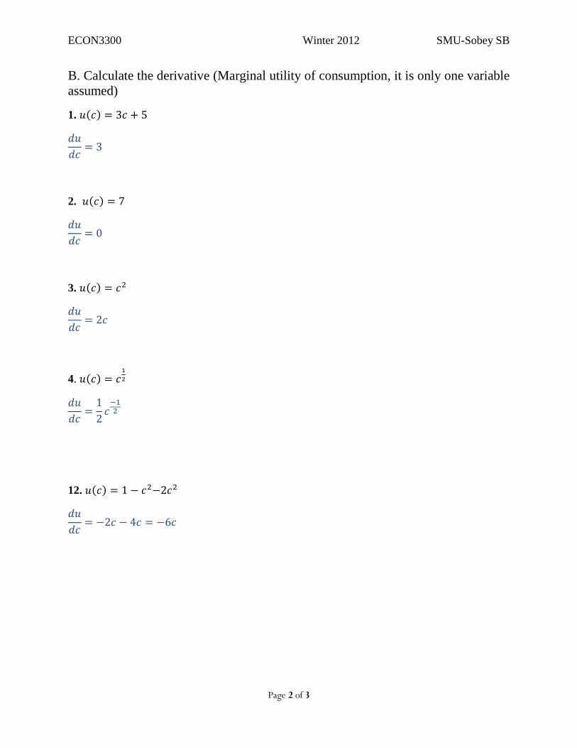
B. Calculate the derivative (Marginal utility of consumption, it is only one variable assumed)

1. 𝑢(𝑐) = 3𝑐 + 5

𝑑𝑢𝑑𝑐

= 3

2. 𝑢(𝑐) = 7

𝑑𝑢𝑑𝑐

= 0

3. 𝑢(𝑐) = 𝑐2

𝑑𝑢𝑑𝑐

= 2𝑐

4. 𝑢(𝑐) = 𝑐12

𝑑𝑢𝑑𝑐

=12𝑐−12

12. 𝑢(𝑐) = 1 − 𝑐2−2𝑐2

𝑑𝑢𝑑𝑐

= −2𝑐 − 4𝑐 = −6𝑐


Page 3 of 3

C.

Answer the following questions.

1. Compare 𝑢(𝑐) = 3𝑐 + 5 and 𝑢(𝑐) = 7 in light of Economic Theory.

Marginal utility of 𝑢(𝑐) = 3𝑐 + 5 is constant which can be a special case but 𝑢(𝑐) = 7 yields a marginal utility equal 0 which is not usually assumed in economics (does not make economic sense).

2. Compare 𝑢(𝑐) = 𝑐12 and 𝑢(𝑐) = 𝑐2 in light of Economic Theory.

Marginal utility of 𝑢(𝑐) = 𝑐12 is decreasing which can be a usual assumption in economics; but

𝑢(𝑐) = 𝑐2 yields an increasing which is not usually assumed in economics.

3. Compare 𝑢(𝑐) = 1 − 𝑐2−2𝑐2 and 𝑢(𝑐) = 𝐶2 in light of Economic Theory.

Marginal utility of 𝑢(𝑐) = 1 − 𝑐2−2𝑐2 = 1 − 3𝑐2 is decreasing corresponding to the is the usual assumption in economics (well-behaved utility functions); but 𝑢(𝑐) = 𝐶2 yields an increasing which is not usually assumed in economics.

ECON3300 SMU-Sobey SB-Winter 2012

Page 1 of 1

Intermediate Microeconomics: Quiz 1

Consider the bundles of goods 𝒙��⃗ ,𝒚��⃗ 𝒂𝒏𝒅 𝒛�⃗ ,𝒃𝒆𝒍𝒐𝒘 and answer the questions.

(i) If Mark 𝒙��⃗ ≫ 𝒚��⃗ then Mark likes Pepsi a lot: T/F/Not sure, why? (ii) If Mark 𝒙��⃗ ≫ 𝒛�⃗ then Mark likes Pepsi a lot: T/F/Not sure, why? (iii) If Mark 𝒚��⃗ ≫ 𝒛�⃗ then Mark likes Pepsi a lot: T/F/Not sure, why?

Pepsi

Burger


Page 1 of 2

Problem Set 1: Definition of Function

Suppose only

1. 𝑦 𝑖𝑠 𝑓𝑢𝑛𝑐𝑡𝑖𝑜𝑛 𝑜𝑓 𝑥 (𝑡ℎ𝑒 𝑟𝑒𝑙𝑎𝑡𝑖𝑜𝑛𝑠ℎ𝑖𝑝 𝑖𝑠 𝑑𝑒𝑠𝑐𝑟𝑖𝑏𝑒𝑑 𝑖𝑛 𝑡ℎ𝑒 𝑡𝑎𝑏𝑙𝑒 𝑏𝑒𝑙𝑜𝑤).

two variables x and y. Label by True, False or Uncertain the statements below. Explain why.

𝑥: number of cows 𝑦: quantity of milk 5 15 5 12 4 12 4 9 3 6

2. 𝑦 𝑖𝑠 𝑓𝑢𝑛𝑐𝑡𝑖𝑜𝑛 𝑜𝑓 𝑥 (𝑡ℎ𝑒 𝑟𝑒𝑙𝑎𝑡𝑖𝑜𝑛𝑠ℎ𝑖𝑝 𝑖𝑠 𝑑𝑒𝑠𝑐𝑟𝑖𝑏𝑒𝑑 𝑏𝑦 𝑡ℎ𝑒 𝑏𝑙𝑎𝑐𝑘 𝑙𝑖𝑛𝑒).

3. The grade of a student, y, is a function of hours this student studies, x.

4. 𝑦 𝑖𝑠 𝑓𝑢𝑛𝑐𝑡𝑖𝑜𝑛 𝑜𝑓 𝑥 (𝑡ℎ𝑒 𝑟𝑒𝑙𝑎𝑡𝑖𝑜𝑛𝑠ℎ𝑖𝑝 𝑖𝑠 𝑑𝑒𝑠𝑐𝑟𝑖𝑏𝑒𝑑 𝑏𝑦 𝑡ℎ𝑒 𝑓𝑜𝑟𝑚𝑢𝑙𝑎 𝑏𝑒𝑙𝑜𝑤).

𝑦 = �𝑥2 𝑖𝑓 𝑥 ≥ 05 𝑖𝑓 𝑥 = 0𝑥3 𝑖𝑓 𝑥 ≤ 0

�


𝑦 = 5


𝑦 − 5𝑥 = −10


𝑦 − �2(𝑥 + 2)2 = 0

0 1 2 3 4 50

2

4

6

8

10

12

x

y


Page 2 of 2


�𝑦 − �2(𝑥 + 2)2 = 0


�𝑦 − 2(𝑥 + 2)2 = 0


𝑦2 = (𝑥 + 2)


𝑦2 = 5



14. The quantity of milk, y, is a function of number of cows, x.

0 1 2 30

1

2

3

x

y

0 1 2 30

1

2

3

x

y


Page 1 of 2

Problem Set 2: Differentiation

We have a function of one variable, denoted by u (in class we used f). The independent variable is c (in class we used x). Compute the derivative of the functions below.

1. 𝑢(𝑐) = 3𝑐 + 5

𝑑𝑢𝑑𝑐

=

2. 𝑢(𝑐) = 7

𝑑𝑢𝑑𝑐

=

3. 𝑢(𝑐) = 𝑐 + 𝐵 (𝐵 𝑖𝑠 𝑎 𝑛𝑢𝑘𝑚𝑏𝑒𝑟)

𝑑𝑢𝑑𝑐

=

4. 𝑢(𝑐) = 𝑐 − 𝐴 (𝐴 𝑖𝑠 𝑎 𝑛𝑢𝑚𝑏𝑒𝑟)

𝑑𝑢𝑑𝑐

=

5. 𝑢(𝑐) = 𝑐2

𝑑𝑢𝑑𝑐

= 2𝑐

6. 𝑢(𝑐) = 𝑐12

𝑑𝑢𝑑𝑐

=


Page 2 of 2

7. 𝑢(𝑐) = 𝑐12

𝑑𝑢𝑑𝑐

=

8. 𝑢(𝑐) = 𝑐

𝑑𝑢𝑑𝑐

=

9. 𝑢(𝑐) = 𝑐−1

𝑑𝑢𝑑𝑐

=

10. 𝑢(𝑐) = −𝐵𝑐 − 𝐴 (𝐴 𝑎𝑛𝑑 𝐵 𝑎𝑟𝑒 𝑛𝑢𝑚𝑏𝑒𝑟𝑠)

𝑑𝑢𝑑𝑐

=

11. 𝑢(𝑐) = 1 − 𝑐2−2𝑐2

𝑑𝑢𝑑𝑐

=

12. 𝑢(𝑐) = 𝐴 − 𝐵 × 𝑐2−𝐷 × 𝑐2 (𝐴,𝐵 𝑎𝑛𝑑 𝐷 𝑎𝑟𝑒 𝑛𝑢𝑚𝑏𝑒𝑟𝑠)

𝑑𝑢𝑑𝑐

=


Page 1 of 6

Notes on Consumer Theory: Demand Function

We know of budget constraints, and preferences summarised in utility function as the basis of

consumer choice. In economics, the function that indicates the quantity chosen by a consumer

given this good’s price (and other variables) demand function.

It results from maximising utility function subject to budget constraint. The demand function we

get after solving such question, are functions of the good’s own price and the decision maker’s

income.

In other words, if the consumer’s problem conceived as such, the solution will give us the

combination of goods (consumer’s basket or bundle) that is situated on the highest utility level

given the prices and income.

Example

Suppose a concave utility function 𝑈(𝑥1, 𝑥2) = 𝑥1𝛼𝑥21−𝛼, The price of good 1 (𝑥1) is 𝑝1 and the

price of good 2 is 𝑝2and his income is m.

Solution

Consumer problem is to choose The Best Possible Bundle.

maximizing 𝒖(𝒙𝟏,𝒙𝟐) = 𝒙𝟏𝜶𝒙𝟐𝟏−𝜶 by choosing 𝑥1 and 𝑥2.

Note: This Utility is Identical to the one used in class: it is regular Cobb-Douglas. Only β is

replaced by (1 − 𝛼). It does not make any difference to the process, it only showcase that the

sum of the exponents is 1.

Subject to budget constraint: 𝒑𝟏 𝒙𝟏 + 𝒑𝟐 𝒙𝟐 = 𝒎.


Page 2 of 6

Note

Marginal utilities are obtained by computing partial derivatives of utility function with respect to

the good under consideration, as follows:

Marginal Utility of 𝑥1 is: 𝑀𝑈1=𝜕𝑢(.)𝜕𝑥1

= 𝛼𝑥1𝛼−1 𝑥21−𝛼

Marginal Utility of 𝑥2 is: 𝑀𝑈2 = 𝜕𝑢(.)𝜕𝑥2

= (1 − 𝛼)𝑥1𝛼 𝑥2−𝛼

The Best Bundle must satisfy: 𝑴𝑼𝟏𝑷𝟏

=𝑴𝑼𝟐𝑷𝟐

𝒚𝒊𝒆𝒍𝒅𝒔�⎯⎯⎯� 𝛼𝑥1

𝛼−1 𝑥21−𝛼

𝒑𝟏=

(1−𝛼)𝑥1𝛼 𝑥2−𝛼

𝒑𝟐 (1)

Note that we can simplify 𝑥1𝛼−1 on the Left-Hand Side (LHS) with 𝑥1𝛼 on the Right-Hand Side

(RHS). It gives us 𝑥1 on the RHS.

Likewise, we can simplify 𝑥21−𝛼 on the LHS with 𝑥2−𝛼 on the RHS. It gives us 𝑥2 on the RHS.

It is so because:

𝑥1𝛼 = 𝑥1𝛼−1 . 𝑥1

(sum the powers to see that).

And likewise:

𝑥21−𝛼 = 𝑥2−𝛼𝑥2

Hence (1) can be re-written as:

𝛼𝑥2𝒑𝟏

=(1 − 𝛼)𝑥1

𝒑𝟐

And with cross-multiplying as isolation 𝑥2 on the LHS we get:

𝒙𝟐 = 𝒑𝟏𝒑𝟐

(𝟏−𝜶)𝜶

𝒙𝟏 (2)

Now, with (2) and the budget constraint we have two equations and two unknowns (𝑥1 𝑎𝑛𝑑 𝑥2),

hence we can solve fore 𝑥1 and 𝑥2. Plugging (2) into BC we get:


Page 3 of 6

𝑚 − 𝑝1 𝑥1 − 𝑝2 𝑥2 = 0𝑦𝑖𝑒𝑙𝑑𝑠�⎯⎯⎯� 𝑚 − 𝑝1 𝒙𝟏 − 𝑝2 �

𝒑𝟏𝒑𝟐

(1 − 𝛼)𝛼

𝑥1 � = 0𝑦𝑖𝑒𝑙𝑑𝑠�⎯⎯⎯�

𝑚 − 𝑝1 𝒙𝟏 − �1−𝛼𝛼� 𝑝1𝑥1 = 0 (keeping the terms with 𝑥1 on one side and m on the other

𝑦𝑖𝑒𝑙𝑑𝑠�⎯⎯⎯�

𝑝1 𝒙𝟏 + �1−𝛼𝛼� 𝑝1𝑥1 = 𝑚 (factorising 𝑝1 𝒙𝟏)


𝑝1 𝒙𝟏 �𝟏 + �1−𝛼𝛼� � = 𝒎 (simplifying the term in the square bracket)


𝑝1 𝒙𝟏 �𝛼+1−𝛼

𝛼 � = 𝒎

𝑦𝑖𝑒𝑙𝑑𝑠�⎯⎯⎯� 𝑝1 𝒙𝟏 �

𝟏𝛼

� = 𝒎

(keeping the terms with 𝑥1 on one side and m on the other) 𝑦𝑖𝑒𝑙𝑑𝑠�⎯⎯⎯�

𝒙𝟏 =𝜶𝒎𝒑𝟏

𝑫𝒆𝒎𝒂𝒏𝒅 𝒇𝒐𝒓 𝒈𝒐𝒐𝒅 𝟏

And likewise:

𝑚 − �𝛼𝑚𝑝1� 𝑝1 − 𝑝2 𝑥2 = 0

𝑦𝑖𝑒𝑙𝑑𝑠�⎯⎯⎯� 𝑚− (𝛼𝑚) − 𝑝2 𝑥2 = 0 (𝑓𝑎𝑐𝑡𝑜𝑟𝑖𝑠𝑖𝑛𝑔 𝑚)


𝑚(1 − 𝛼) − 𝑝2 𝑥2 = 0

keeping the term with 𝑥2 on one side we get:

𝑚(1 − 𝛼) = 𝑝2 𝑥2

And finally, isolating 𝑥2 we have:

𝒙𝟐 =(𝟏 − 𝜶)𝒎

𝒑𝟐 𝑫𝒆𝒎𝒂𝒏𝒅 𝒇𝒐𝒓 𝒈𝒐𝒐𝒅 𝟐


Page 4 of 6

NOTE Optional

(i) You see that our demands verify the Law of Demand:

𝜕𝑥1𝜕𝑝1

=𝜕�𝛼𝑚𝑝1

�

𝜕𝑝1= 𝜕�𝛼𝑚𝑝1−1�

𝜕𝑝1=(-1) 𝛼𝑚𝑝1−2 < 0

As α ∈ (0,1) and prices cannot be negative the partial derivative of demand for 𝑥1 with respect to 𝒑𝟏 is negative.

You can do it for 𝑥2 as an exercise.

(ii) You see that our demands verify the usual relationship between normal goods and income which postulates that as income rises the consumption of a normal good rise:

𝜕𝑥1𝜕𝑚

=𝜕 �𝛼𝑚𝑝1

�

𝜕𝑚=𝛼 𝑝1

> 0

As α ∈ (0,1) and prices cannot be negative the partial derivative of demand for 𝑥1 with respect to m is positive.

You can do it for 𝑥2 as an exercise.


Page 5 of 6

Graphic Representation

So what are we really doing when we use Lagrange method to get the demands?

Suppose (𝑥1, 𝑥2) = 𝑥112𝑥2

12 . Solving for demands we get:

𝒙𝟏 =𝒎𝟐𝒑𝟏

𝒙𝟐 = 𝒎𝟐𝒑𝟐

These functions will give the quantity demanded for a given income and a given set of prices. If prices change the quantities will change as well.

Now suppose 𝑝1 = 2 and 𝑝2 = 1 and 𝑚 = 24; Then 𝒙𝟏 = 𝟔 and 𝒙𝟐 = 𝟏𝟐

The choice is represented below:

Now suppose the price of good 1 falls to 1: 𝑝1 = 1

Law of demand says that the consumption of good 1 has to fall. It does indeed (plys new price into the demand function): 𝒙𝟏 = 𝟏𝟐 and 𝒙𝟐 = 𝟏𝟐

And graphically:

Now let’s put the two situations (𝑝1 = 2 ∶ 𝑆𝑜𝑙𝑖𝑑 𝑙𝑖𝑛𝑒𝑠 𝑎𝑛𝑑 𝑝1 = 1: 𝐷𝑎𝑠ℎ𝑒𝑑 𝑙𝑖𝑛𝑒𝑠) along the demand function for 𝑥1 in another figure (blue curve).

0 2 4 6 8 10 12 14 16 18 20 22 240

5

10

15

20

x1

x2

0 2 4 6 8 10 12 14 16 18 20 22 240

5

10

15

20

x1

x2


Page 6 of 6

0 2 4 6 8 10 12 14 16 18 20 22 240

5

10

15

20

x1

x2

0 1 2 3 4 5 6 7 8 9 10 11 12 13 140

5

10

15

20

25

x1

p1


Page 1 of 1

Problem Set, Intratemporal choice


Suppose that in a given economy, there is only two periods: Present and Future to allocate life-time income. Answer the following questions

(i) What is the microeconomics framework you will use to explore this question?

(ii) State the appropriate Utility Function and Budget Constraint.

(iii) Derive the demand function for consumption in Present.

(iv) Provide an illustration depicting the choice.

(v) Using you answer to the part (iii), explain what you expect to happen if Real Interest Rate increase.

(vi) Using you answer to the part (iii), explain what you expect to happen if the decision maker becomes less patient.

(vii) Explain how the framework used to answer this question differs from that of a choice between Coffee and Donuts.


Page 1 of 6

Questions on Intratemporal choice: Answer Key


Suppose that in a given economy, there is only two periods: Present and Future to allocate life-time income. Answer the following questions

(i)

What is the microeconomics framework you will use to explore this question?

Consumer theory for Intertemporal Choice ⤇ Maximizing Utility Subject to Budget Constraint; adapting the utility function and the budget constraint to the specificities of the Intratemporal Choice question.

(ii)

State the appropriate Utility Function and Budget Constraint.

Utility Function:

𝑢(𝑐1, 𝑐2) = ln(𝑐1) + β ln(𝑐2)

With 0 < 𝛽 < 1 and 𝑐1:𝐶𝑜𝑛𝑠𝑢𝑚𝑝𝑜𝑡𝑖𝑜𝑛 𝑖𝑛 𝑃𝑟𝑒𝑠𝑒𝑛𝑡; 𝑐2:𝐶𝑜𝑛𝑠𝑢𝑚𝑝𝑜𝑡𝑖𝑜𝑛 𝑖𝑛 𝐹𝑢𝑡𝑢𝑟𝑒

And assuming the interest rate is i (alternatively you can use r) income in Present is 𝑦1 and income in Future is 𝑦2, t then Budget constraint becomes:

𝑐1 + �1

1 + 𝑖� 𝑐2 = 𝑦1 + �

11 + 𝑖

� 𝑦2

(iii)

Derive the demand function for consumption in Present.

The following steps are required:

Maximising Utility by choosing 𝑐1 𝑎𝑛𝑑 𝑐2 subject to Budget constraint.

1. Question:

2. Mathematical Expression:


Page 2 of 6

max𝑐1,𝑐2 𝑢(𝑐1, 𝑐2) 𝑠. 𝑡.

𝑐1 + � 11+𝑖� 𝑐2 = 𝑦1 + � 1

1+𝑖� 𝑦2 ⤇

3. Finding the tangency

⤇ 𝑀𝑈(𝑐1)𝑀𝑈(𝑐2)

= 1�1 1+𝑖� �

⤇

1 𝑐1⁄𝛽(1 𝑐2⁄ ) =

1�1

1 + 𝑖� � ⤇

𝑐2𝛽𝑐1

= 1 + 𝑖

between the Indifference Curve (curve, utility function) and the Budget Constraint (straight line) ⤇

𝑀𝑅𝑆 = 𝑅𝑒𝑙𝑎𝑡𝑖𝑣𝑒 𝑃𝑟𝑖𝑐𝑒: �𝑃𝑟𝑖𝑐𝑒 𝑜𝑓 𝐺𝑜𝑜𝑑 𝑜𝑛 𝑡ℎ𝑒 𝑥 − 𝑎𝑥𝑖𝑠𝑃𝑟𝑖𝑐𝑒 𝑜𝑓 𝐺𝑜𝑜𝑑 𝑜𝑛 𝑡ℎ𝑒 𝑦 − 𝑎𝑥𝑖𝑠

�

Equation-1 is then:

Cross-multiplying to isolate 𝑐1 𝑎𝑛𝑑 𝑐2 𝑖𝑛 𝑡ℎ𝑒 𝐿𝑒𝑓𝑡 𝐻𝑎𝑛𝑑 𝑆𝑖𝑑𝑒 (𝐿𝐻𝑆)

�𝑬𝒒𝒖𝒂𝒕𝒊𝒐𝒏 𝟏.𝟏: 𝒄𝟐 = 𝜷(𝟏 + 𝒊)𝒄𝟏𝑬𝒒𝒖𝒂𝒕𝒊𝒐𝒏 𝟏.𝟐: 𝒄𝟏 =

𝒄𝟐𝜷(𝟏 + 𝒊)

�

𝒄𝟐𝜷𝒄𝟏

= 𝟏 + 𝒊 ⤇

4. Using Equations 1.1. and 1.2 with the budget constrain

t to find Demand functions.

Important Note:

For Demand for 𝑐1 we substitute for 𝑐2 in the Budget constraint.

demand function must only incorporate the parameters: the parameters of the utility function like β and/or α, prices and incomes. Here they are i and 𝑦1.,𝑦2.,𝑎𝑛𝑑 β are i and 𝑦1.,𝑦2.,𝑎𝑛𝑑 β.

Budget constraint: 𝒄𝟏 + � 𝟏𝟏+𝒊� 𝒄𝟐 = 𝒚𝟏 + � 𝟏

𝟏+𝒊� 𝒚𝟐 : Equation 2

𝑐1 + �1

1 + 𝑖� 𝑐2 = 𝑦1 + �

11 + 𝑖

� 𝑦2𝑠𝑢𝑏 1.1��

𝑐1 + �1

1 + 𝑖� (𝛽(1 + 𝑖)𝑐1) = 𝑦1 + �

11 + 𝑖

� 𝑦2


Page 3 of 6

𝐴𝑙𝑔𝑒𝑏𝑟𝑎 ��

𝑐1 + �1

1 + 𝑖� (𝛽(1 + 𝑖)𝑐1) = 𝑦1 + �

11 + 𝑖

� 𝑦2


𝑐1 + 𝛽𝑐1 = 𝑦1 + �1

1 + 𝑖� 𝑦2


𝑐1(1 + 𝛽) = 𝑦1 + �1

1 + 𝑖� 𝑦2


𝑐1 = �𝑦1 + �1

1 + 𝑖� 𝑦2� �

11 + 𝛽

�


𝑐1 =�𝑦1 + � 1

1 + 𝑖� 𝑦2�1 + 𝛽

Note: If you have trouble with algebra leave it as it is: up to this step is adequate and gets full mark: it is a Demand Function for it only includes parameters: i, β, 𝑦1 𝑎𝑛𝑑 𝑦2.


𝑐1 =[𝑦1 + (1 + 𝑖)𝑦2](1 + 𝛽)(1 + 𝑖)

(iv)

Provide an illustration depicting the choice.

It is like the Cobb-Douglas ones you have seen before.

(v)

Using you answer to the part (iii), explain what you expect to happen if Real Interest Rate increases.

Real interest rate goes up : i↑ ⤇


Page 4 of 6

𝑐1 =�𝑦1 + � 1

1 + 𝑖 ↑� 𝑦2�

1 + 𝛽

⤇

𝑐1 =�𝑦1 + � 1

1 + 𝑖� 𝑦2 ↓�1 + 𝛽

⤇ 𝑐1 ↓

Intuition and Economic Reason

(vi) Using you answer to the part (iii), explain what you expect to happen if the decision maker becomes less patient.

: If i↑⤇ it is more rewarding to save ⤇ to save c_1↓: one must consume less in Present to save for Future.

Less patient consumer ⤇β↓ : higher β means future is similar to Present for the consumer, the extreme is β=1: making no difference between Present and Future.

So we have:

Less patient consumer ⤇β↑⤇

𝑐1 =�𝑦1 + � 1

1 + 𝑖� 𝑦2�1 + 𝛽 ↓

⤇

𝑐1 =�𝑦1 + � 1

1 + 𝑖� 𝑦2�1 + 𝛽 ↓

⤇

𝑐1 =�𝑦1 + � 1

1 + 𝑖� 𝑦2�1 + 𝛽

↑

⤇ 𝑐1 ↑

Intuition and Economic Reason: If 𝛽 ↓: less patient, then obviously, this consumer will consumer and Present and will not save/wait to consume in the future.

For coffee and Cookies we usually use Cobb- Douglas utility functions:

𝑼(𝒙𝟏,𝒙𝟐) = 𝒙𝟏𝜶𝒙𝟐𝟏−𝜶


Page 5 of 6

And Marginal Utility of 𝑥1 (𝑥2) is a function of 𝑥1 (𝑥2) while it is not the case with Log Utility (used for Intratemporal Choice).

𝑴𝒂𝒓𝒈𝒊𝒏𝒂𝒍 𝑼𝒕𝒊𝒍𝒊𝒕𝒚 𝒐𝒇 𝒙𝟏 =𝝏𝒖(. )𝝏𝒙𝟏

= 𝟑𝒙𝟏𝟐𝒙𝟐𝟑


𝑴𝒂𝒓𝒈𝒊𝒏𝒂𝒍 𝑼𝒕𝒊𝒍𝒊𝒕𝒚 𝒐𝒇 𝒙𝟐 =𝝏𝒖(. )𝝏𝒙𝟐

= 𝟑𝒙𝟐𝟐𝒙𝟏𝟑

Note

While for 𝑢(𝑐1, 𝑐2) = ln(𝑐1) + β ln(𝑐2)

𝑀𝑎𝑟𝑔𝑖𝑛𝑎𝑙 𝑈𝑡𝑖𝑙𝑖𝑡𝑦 𝑜𝑓 𝑐1 =𝜕𝑢(. )𝜕𝑐1

=1𝑐1

𝑀𝑎𝑟𝑔𝑖𝑛𝑎𝑙 𝑈𝑡𝑖𝑙𝑖𝑡𝑦 𝑜𝑓 𝑐2 =𝜕𝑢(. )𝜕𝑐2

=𝛽𝑐2

: Here, it is as-if we are differentiation "𝐴. 𝑥23" with respect to 𝑥2 where A=𝑥13

The Log (ln) utility function is more sensible for inter-temporal choice and the consumptions are not at the same time and usually regarded as independent by the consumers. But with the Coffees and Cookies, they are consumed together and it makes sense to assume that the consumer’s marginal utility from the quantity of the Cookies consumed depends on the quantity of coffees she has.

Intuition and Economic Reason:

**&**

And as exercise, you can try the case for decrease in the interest rate and more patients people.

Good Luck! Dr. Maryam Dilmaghani


Page 6 of 6


Page 1 of 1

Production Costs & Cost Minimization Instructor: Dr. Maryam Dilmaghani

The figures below describe the production process of Fictional Ltd. Output is produced using labour (L) and capital (K). The iso-quant (the curve) depicts different combinations of L and K that will let the firm producing 1000 unit (Q=1000), the decision made by the CEO. The the straight lines are iso-costs: different combinations of L and K that cost the same thing to the firm. Look at the figures below and answer the questions.

1. Find the least cost combination of L and K to produce the quantity decided by the CEO.

2. If the wage of units of labour is $100, what is the least cost of producing Q=100?

As you see in the figure above wage increase. Now unit cost of labour is $120.

3. Would you advise the firm to continue with the same combination of inputs? Why?

4. What can you tell about the least cost combination of inputs?

0 1 2 3 4 5 6 7 8 9 10 11 120

2

4

6

8

10

12

14

L

K

0 1 2 3 4 5 6 7 8 9 10 11 120

2

4

6

8

10

12

14

16

L

K

ECON3300: SMU Due February 5th, 2012; Beginning of the lecture

Page 1 of 1

Last Name/ First Name/ Student ID:

Assignment 1: Consumer Theory


General Guidelines 1. No late assignment will be accepted unless there is a medical excuse. 2. Assignment should be submitted individually. 3. Respect the length indicated for answers if applicable 4. Show your work if applicable.

(no more than the limit will be read).

A.

Ms. Pandora’ satisfaction from consumption is a function of the number of concerts she attends in a year (𝑑𝑒𝑛𝑜𝑡𝑒𝑑 𝑏𝑦 𝑥1) and the amount of money

Suppose the price of 𝑥1 is 𝒑𝟏 and Pandora’s income is 𝒎 𝒅𝒐𝒍𝒍𝒂𝒓𝒔.

she disposes to spend on all other goods (𝑑𝑒𝑛𝑜𝑡𝑒𝑑 𝑏𝑦 𝑥2). It is expressed below.

𝒖(𝒙𝟏 ,𝒙𝟐) =𝒎𝟐𝟎

𝒙𝟏 −𝒙𝟏𝟐

𝟐+ 𝒙𝟐


(i) Depict Ms. Pandora’s budget constraint if the average price of concert tickets is $75 and her income $1600.

Hint: Note that, Price of money is 1, in other words we have 𝑝2 = 1.

(ii) Depict Ms. Pandora’s budget constraint if the average price of concert tickets is $75 and her income $3200.

(iii) Depict Ms. Pandora’s budget constraint if the average price of concert tickets is $100 and her income $1600?

(iv) Depict Ms. Pandora’s budget constraint if the average price of concert tickets is $30 and her income $1600?

(v) Compare the budget set in part (i) with (ii), (iii), (iv).


Page 1 of 1



Part B.

Recall from Part A:




𝒖(𝒙𝟏 ,𝒙𝟐) =𝒎𝟐𝟎

𝒙𝟏 −𝒙𝟏𝟐

𝟐+ 𝒙𝟐


(i)

For an income $1600 (m=1600), sketch an indifference curve that will give Ms. Pandora a utility equal 1600 utiles (unit of measurement of utility).

Hint: You need to fine different combination of cash and number of concerts that will leave Ms. Pandora indifferent among them.

(ii)


(iii)

What can you tell about the rate of substitution of Ms. Pandora between Money and Concert?

(iv)

Ms. Pandora’s best friend, Ms. Artemis, likes attending the concerts more that Ms. Pandora. What would you propose to be changed in Ms. Pandora’s utility function to represent that of Ms. Artemis?

(v) How would you compare the utility function below to that of Ms. Pandora? Comment!

𝒖(𝒙𝟏 ,𝒙𝟐) =𝒎𝟐𝟎

𝒙𝟏 + 𝒙𝟐


Page 1 of 2



Part B.

Recall from Part A:




𝒖(𝒙𝟏 ,𝒙𝟐) =𝒎𝟐𝟎

𝒙𝟏 −𝒙𝟏𝟐

𝟐+ 𝒙𝟐


(i)


Hint: These preferences are called Quasi-Linear.

To answer the question, you need to fine different combination of cash and number of concerts that will leave Ms. Pandora indifferent among them and give a utility of 80 utiles:

𝒖(𝒙𝟏 ,𝒙𝟐) =𝒎𝟐𝟎

𝒙𝟏 −𝒙𝟏𝟐

𝟐+ 𝒙𝟐 ⤇ 𝟖𝟎 =

𝟏𝟔𝟎𝟎𝟐𝟎

𝒙𝟏 −𝒙𝟏𝟐

𝟐+ 𝒙𝟐

And you can continue by filling the table below to have the points:

𝒙𝟏 𝒙𝟐

0 𝟖𝟎 =𝟏𝟔𝟎𝟎𝟐𝟎

× 𝟎 −𝟎𝟐

+ 𝒙𝟐

You continue... You continue...


Page 2 of 2

(ii)


(iii)

What can you tell about the rate of substitution of Ms. Pandora between Money and Concert?

(iv)

Ms. Pandora’s best friend, Ms. Artemis, likes attending the concerts more that Ms. Pandora. What would you propose to be changed in Ms. Pandora’s utility function to represent that of Ms. Artemis?

(v) How would you compare the utility function below to that of Ms. Pandora? Comment!

𝒖(𝒙𝟏 ,𝒙𝟐) =𝒎𝟐𝟎

𝒙𝟏 + 𝒙𝟐

ECON3300: SMU Due March 21st, 2012; Beginning of the lecture

Page 1 of 2


Assignment 2&3: Producer Theory




A.

Part A

The company FarmaC, produces pharmaceutics using Capital and Labour. It production process

can be expressed by the Cobb-Douglas function below.

𝑄 = 𝐴𝐹(𝐾, 𝐿) = 𝐿23𝐾

13

So: 𝐴 = 1, 𝛼 = 23

⤇ 𝛼 − 1 = −13

,𝛽 = 13

⤇ 𝛽 − 1 = −23


1.

Compute the Marginal Products of inputs (MPL and MPK).

2.

Compute the Marginal Rate of Transformation MRT).

3.

Derive the input demand function conditional on having the output Q=1000 units.

Provide a

4.

figure.

If the pharmaceutical market is competitive, what can you tell about FarmaC’s profits? Write down the profit function

.

ECON3300: SMU Due March 21st, 2012; Beginning of the lecture

Page 2 of 2

Part B.

After some changes taking place in the market, now FarmaC is a monopoly is pharmaceutics market, the only firm producing a class of chemicals. Demand (willingness to pay: WTP) and Marginal cost (supply) are given below:

�𝐷 (𝑊𝑇𝑃): 𝑃𝑑 = 100 − 𝑄𝑑

𝑆 (𝑀𝐶): 𝑃𝑠 = 10 + 𝑄𝑠 �

1.

You consulted by this firm about the quantity to produce and the selling price. How will you answer to the firm’s executives? Provide a

figure.

2.

What is the monopolistic profit of this firm, provided that

Quantity

ATC is given in the Table below?

ATC 5 $75

10 $65 30 $58 45 $55

3.

Calculate the Dead Weight Loss (DWL) of this Monopoly?

4.

How this monopolists’ profit will change if the firm’s executives were able to charge the first 10 buyers their total willingness to pay? Provide a

figure.

ECON3300: SMU Due April 4th, 2012; 5:00 pm

Page 1 of 1


The Last Assignment: Market Structure




Fictional Ltd. is a firm producing a class of chemicals. Demand (willingness to pay: WTP) and the Total Cost function are given below:

� 𝐷 (𝑊𝑇𝑃): 𝑃 = 32 − 𝑄𝑇𝑜𝑡𝑎𝑙 𝐶𝑜𝑠𝑡𝑠 (𝑄) = 10 + 𝑄

�

Answer the flowing question.

1. Suppose the market for this class of Chemical is perfectly competitive, find the market

Equilibrium. Illustrate.

2. Suppose that Fictional Ltd. is a monopoly, the only firm in this market, find the market

Equilibrium. Illustrate.

3. Suppose that Fictional Ltd. is one of the two firms in this market, compositing with FarmaC, a

firm with identical technology hence cost functions. Find the market Equilibrium in a Cournot

competition.

4. Now suppose that Fictional Ltd. is the Stackelberg leader of the market. Find the market

Equilibrium.

5. Rank the market equilibrium values of the abode questions, in terms of the consumer surplus.

Briefly justify your ranking.

Good Luck!

MD

SMU- SSB: ECON3300 Winter 2012

Page 1 of 4

Assignment Tips: Monopoly


Fictional Ltd. is the only firm producing a class of chemicals. You consulted by this firm about the quantity to produce and the selling price. Demand (willingness to pay: WTP) and Marginal cost (supply) are given below:

�𝐷 (𝑊𝑇𝑃): 𝑃𝑑 = 100 − 𝑄𝑑

𝑆 (𝑀𝐶): 𝑃𝑠 = 10 + 𝑄𝑠 �

1. How will you answer to the firm’s executives?

A monopolist

Answer:

chooses the quantity to put into the market in order to maximize its profit

Hence, we need to first find MR function (curve: dashed, blue).

𝐷: 𝑃𝑑 = 100 − 𝑄𝑑 ⇒ 𝑀𝑅 = 100 − 2𝑄𝑑

𝑀𝑅 = 𝑀𝐶 ⇒ ….

“given the impact of the quantity supplied on the consumer’s willingness to pay”. To maximize profits requires setting: 𝑀𝑅 = 𝑀𝐶

As we see below, this means a lower quantity and a higher price compared to perfect competition outcome:

0 10 20 30 40 50 60 70 80 90 1000

10

20

30

40

50

60

70

80

90

100

Q

P


Page 2 of 4

𝐷 = 𝑆 ⇒ ….

2. What is the monopolistic profit of this firm, provided that

Quantity

ATC is given in the Table below.

ATC 5 $75

10 $65 30 $58 45 $55

Step 1: Finding Total Costs (TC)

𝑇𝐶 = 𝐴𝑇𝐶 ∗ 𝑄 = ⋯

Step 3: Finding Total Revenue (TR)

𝑇𝑅 = 𝑃𝑀 ∗ 𝑄 = ⋯

Step 4: Finding Profits (𝝅)

𝜋 = 𝑇𝑅 − 𝑇𝐶 = ⋯

0 10 20 30 40 50 60 70 80 90 1000

10

20

30

40

50

60

70

80

90

100

Q

P

ATC Profits


Page 3 of 4

3. What is the Dead Weight Loss (DWL) of this Monopoly?

Dead Weight Loss is the quantity for which Willingness to pay of the consumers (demand) is larger than willingness to accept o producers, yet this quantity is not exchanged in the market.

Step 1: Finding MC at 𝑸 = 𝟑𝟎

𝑀𝐶: 𝑃𝑠 = ⋯

Step 2: Finding the basis of triangle (DWL)

It is noted by the vertical curly bracket: 𝐵𝑎𝑠𝑖𝑠 = ⋯

Step 3: Finding the height of triangle (DWL)

It is noted by the horizontal curly bracket: 𝐻𝑒𝑖𝑔ℎ𝑡 = ⋯

Step 4: Finding the Dead Weight Loss (DWL)

It is noted by the area of the shaded triangle:

𝐴 =𝐻𝑒𝑖𝑔ℎ𝑡 ∗ 𝐵𝑎𝑠𝑖𝑠

2= ⋯

0 10 20 30 40 50 60 70 80 90 1000

10

20

30

40

50

60

70

80

90

100

Q

P DWL


Page 4 of 4

4. How this monopolists’ profit will change if the firm’s executives were able to charge the first 10 buyers their total willingness to pay

?

We see that it has increased!

It can be computed by adding the three shaded shapes in the above, it leads to:

𝑁𝑒𝑤 𝑃𝑟𝑜𝑓𝑖𝑡𝑠 = 𝐴𝑑𝑑𝑖𝑜𝑛𝑎𝑙 𝑃𝑟𝑜𝑓𝑡 𝑓𝑟𝑜𝑚 𝑃𝑟𝑖𝑐𝑒 𝐷𝑖𝑠𝑐𝑟𝑖𝑚𝑖𝑛𝑎𝑡𝑖𝑜𝑛 + 𝑂𝑙𝑑 𝑃𝑟𝑜𝑓𝑖𝑡𝑠

𝑁𝑒𝑤 𝑃𝑟𝑜𝑓𝑖𝑡𝑠 = ⋯.

So with this price discrimination, profits have increased by…

0 10 20 30 40 50 60 70 80 90 1000

10

20

30

40

50

60

70

80

90

100

Q

P Profit

ECON3300 Instructor: Dr. Maryam Dilmaghani

Page 1 of 4

Assignment Tips: Monopoly

Fictional Ltd. is the only firm producing a class of chemicals. You consulted by this firm about the quantity to produce and the selling price. Demand (willingness to pay: WTP) and Marginal cost (supply) are given below:

�𝐷 (𝑊𝑇𝑃): 𝑃𝑑 = 100 − 𝑄𝑑

𝑆 (𝑀𝐶): 𝑃𝑠 = 10 + 𝑄𝑠 �

1. How will you answer to the firm’s executives?

A monopolist

Answer:

chooses the quantity to put into the market in order to maximize its profit

Hence, we need to first find MR function (curve: dashed, blue).

𝐷: 𝑃𝑑 = 100 − 𝑄𝑑 ⇒ 𝑀𝑅 = 100 − 2𝑄𝑑

𝑀𝑅 = 𝑀𝐶 ⇒ 100 − 2𝑄 = 10 + 𝑄 ⇒ 𝑄 = 30

𝑄 = 30 ⇒ 𝑊𝑇𝑃 = 𝑃𝑀 = 100 − 30 = $70

“given the impact of the quantity supplied on the consumer’s willingness to pay”. To maximize profits requires setting: 𝑀𝑅 = 𝑀𝐶

0 10 20 30 40 50 60 70 80 90 100

0

10

20

30

40

50

60

70

80

90

100

Q

P


Page 2 of 4

As we see below, this means a lower quantity and a higher price compared to perfect competition outcome:

𝐷 = 𝑆 ⇒ 100 − 𝑄 = 10 + 𝑄 ⇒ 𝑄 = 45 ⇒ 𝑀𝐶 = 𝑃 = 10 + 45 = $55

2. What is the monopolistic profit of this firm, provided that

Quantity

ATC is given in the Table below.

ATC 5 $75

10 $65 30 $58 45 $55

Step 1: Finding Total Costs (TC)

𝑇𝐶 = 𝐴𝑇𝐶 ∗ 𝑄 = 30 ∗ 58 = $1740

Step 3: Finding Total Revenue (TR)

𝑇𝑅 = 𝑃𝑀 ∗ 𝑄 = 30 ∗ 70 = $2100

Step 4: Finding Profits (𝝅)

𝜋 = 𝑇𝑅 − 𝑇𝐶 = $2100− $1740 = $360

0 10 20 30 40 50 60 70 80 90 1000

10

20

30

40

50

60

70

80

90

100

Q

P

ATC Profits


Page 3 of 4

So this monopolist profits are $𝟑𝟔𝟎.

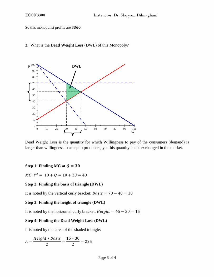
3. What is the Dead Weight Loss (DWL) of this Monopoly?

Dead Weight Loss is the quantity for which Willingness to pay of the consumers (demand) is larger than willingness to accept o producers, yet this quantity is not exchanged in the market.

Step 1: Finding MC at 𝑸 = 𝟑𝟎

𝑀𝐶: 𝑃𝑠 = 10 + 𝑄 = 10 + 30 = 40

Step 2: Finding the basis of triangle (DWL)

It is noted by the vertical curly bracket: 𝐵𝑎𝑠𝑖𝑠 = 70 − 40 = 30

Step 3: Finding the height of triangle (DWL)

It is noted by the horizontal curly bracket: 𝐻𝑒𝑖𝑔ℎ𝑡 = 45 − 30 = 15

Step 4: Finding the Dead Weight Loss (DWL)

It is noted by the area of the shaded triangle:

𝐴 =𝐻𝑒𝑖𝑔ℎ𝑡 ∗ 𝐵𝑎𝑠𝑖𝑠

2=

15 ∗ 302

= 225

0 10 20 30 40 50 60 70 80 90 1000

10

20

30

40

50

60

70

80

90

100

Q

P DWL


Page 4 of 4

4. How this monopolists’ profit will change if the firm’s executives were able to charge the first 10 buyers their total willingness to pay

?

We see that it has increased!

It can be computed by adding the three shaded shapes in the above, it leads to:

𝑁𝑒𝑤 𝑃𝑟𝑜𝑓𝑖𝑡𝑠 = �10 ∗ 10

2� + [10 ∗ 20] + 𝑂𝑙𝑑 𝑃𝑟𝑜𝑓𝑖𝑡𝑠

𝑁𝑒𝑤 𝑃𝑟𝑜𝑓𝑖𝑡𝑠 = $50 + $200 + $360 = $𝟔𝟏𝟎

So with this price discrimination, profits have increased by 250360

× 100 ≈ 70%.

0 10 20 30 40 50 60 70 80 90 1000

10

20

30

40

50

60

70

80

90

100

Q

P Profit

ECON3300: SMU, Winter 2012

Page 1 of 1

Midterm Exam Sample

Prof. Maryam Dilmaghani

1. What are the main assumptions made about economic agents? Briefly elaborate on their meaning.

2. Briefly explain what you know about the preference relationship (their aim and their properties).

3. Using an illustration, explain what is meant by Budget Constraint.

4. Using a figure, explain what is represented by an Indifference Curve.

5. Using a figure, explain what is represented by the Indifference Map (set of the Indifference Curves).

6. Briefly explain what is the goal of using a utility function.

7. What is meant by the Marginal Rate of Substitution (MRS).

8. Using an illustration, represent the preferences of an agent about two goods she finds as perfect substitutes (e.g. 1 litre and 2 litre bottles of Pepsi).

9. Using an illustration, represent the preferences of an agent about two goods she finds as perfect complements (e.g. coffee and sugar).

10. Using an illustration, represent the most general well-behaved references.

11. Ms. Pandora’ satisfaction from consumption is a function of the number of concerts she attends in a year (𝑑𝑒𝑛𝑜𝑡𝑒𝑑 𝑏𝑦 𝑥1) and the amount of money

(i) How can it be changed to represent the preferences of someone who likes going to concerts less than Miss Pandora?


𝒖(𝒙𝟏 ,𝒙𝟐) =𝒎𝟐𝟎

𝒙𝟏 −𝒙𝟏𝟐

𝟐+ 𝒙𝟐

(ii) How can it be changed to represent the preferences of someone who has no Reservation Price (maximum willingness to pay) for concert?

12. How would you suggest to change the utility unction above if was to represent Miss Pandora’s preferences over expenses on housing and food? What about concert and sport match?

Midterm ECON3300 - Time: 70 Minutes February 15th, 2012

Page 1 of 6

Last Name: First Name: Student Number: Major:

General Guidelines

1. Write down your identification in the places assigned. 2. Illegible answers will not be read. 3. Calculator and dictionaries are allowed.

Mark (/100) Don’t write anything in here.

Ms. Athena’s utility function, defined over the two types of consumption goods relevant to her spending decisions, is represented by 𝑼(𝒙𝟏,𝒙𝟐) = 𝒙𝟏𝜶𝒙𝟐𝟏−𝜶 with 𝟎 < 𝛼 < 1. The price of good 1 (𝑥1) is 𝑝1 and the price of good 2 is 𝑝2and his income is m. Answer the following questions.

(i) What can you tell about the type of goods

1. Goods for which a consumer will never choose a zero level of consumption, such as housing and transportation, food and health etc.

that 𝑥1 and 𝑥2 are in terms of the rate of substitution between them? Out of 10

2. Non-constant rate of substitution

3. Decreasing Marginal Utility of consumption for both goods.

(ii) Compute the Marginal Rate of Substitution (MRS). What is the main feature

𝑀𝑎𝑟𝑔𝑖𝑛𝑎𝑙 𝑈𝑡𝑖𝑙𝑖𝑡𝑦 𝑜𝑓 𝑥1 = 𝑀𝑈 (𝑥1) = 𝜕𝑈(.)𝜕𝑥1

= 𝛼𝒙𝟏𝜶−𝟏(𝒙𝟐𝟏−𝜶 )

of this MRS? Out of 15

𝑀𝑅𝑆 =𝑀𝑎𝑟𝑔𝑖𝑛𝑎𝑙 𝑈𝑡𝑖𝑙𝑖𝑡𝑦 𝑜𝑓 𝑥1𝑀𝑎𝑟𝑔𝑖𝑛𝑎𝑙 𝑈𝑡𝑖𝑙𝑖𝑡𝑦 𝑜𝑓 𝑥2

𝑀𝑎𝑟𝑔𝑖𝑛𝑎𝑙 𝑈𝑡𝑖𝑙𝑖𝑡𝑦 𝑜𝑓 𝑥2 = 𝑀𝑈 (𝑥2) = 𝜕𝑈(.)𝜕𝑥2

= (1 − 𝛼)𝒙𝟐−𝜶(𝒙𝟏𝜶)

𝑀𝑅𝑆 =𝛼𝒙𝟏𝜶−𝟏(𝒙𝟐𝟏−𝜶 )

(1 − 𝛼)𝒙𝟐−𝜶(𝒙𝟏𝜶)=

𝛼𝒙𝟐(1 − 𝛼)𝒙𝟏

Features:

Non-constant rate of substitution: Decreasing as the quantity consumed of the good on the x-axis (𝑥1), increases.


Page 2 of 6

(iii) Write down Ms. Athena’s the Budgets constraint and represent it in an illustrative figure if 𝒑𝟏 = 𝒑𝟐 = 𝟏, recall that m=$100. Out of 10

𝑝1𝑥1 + 𝑝2𝑥2 = 𝑚 ⤇ 𝑥1 + 𝑥2 = 100

(iv) Suppose 𝛼 = 12 and derive the Demand Function

To get the demand, we use the optimality condition and the budget constraint.

for 𝑥1. Illustrate it with a figure.

Out of 25

𝑴𝑼𝟏𝑷𝟏

=𝑴𝑼𝟐𝑷𝟐

𝒚𝒊𝒆𝒍𝒅𝒔�⎯⎯⎯� 𝛼𝑥1

𝛼−1 𝑥21−𝛼

𝒑𝟏=

(1−𝛼)𝑥1𝛼 𝑥2−𝛼

𝒑𝟐 (1)

Hence (1) can be re-written as:

𝛼𝑥2𝒑𝟏

=(1 − 𝛼)𝑥1

𝒑𝟐

And with cross-multiplying as isolation 𝑥2 on the LHS we get:

𝒙𝟐 = 𝒑𝟏𝒑𝟐

(𝟏−𝜶)𝜶

𝒙𝟏 (2)

0 10 20 30 40 50 60 70 80 90 1000

10

20

30

40

50

60

70

80

90

100

x1

x2


Page 3 of 6

Now, with (2) and the budget constraint we have two equations and two unknowns

(𝑥1 𝑎𝑛𝑑 𝑥2), hence we can solve fore 𝑥1 and 𝑥2. Plugging (2) into BC we get:

𝑚 − 𝑝1 𝑥1 − 𝑝2 𝑥2 = 0𝑦𝑖𝑒𝑙𝑑𝑠�⎯⎯⎯� 𝑚 − 𝑝1 𝒙𝟏 − 𝑝2 �

𝒑𝟏𝒑𝟐

(1 − 𝛼)𝛼

𝑥1 � = 0𝑦𝑖𝑒𝑙𝑑𝑠�⎯⎯⎯�

𝑚 − 𝑝1 𝑥1 − �1−𝛼𝛼� 𝑝1𝑥1 = 0 (keeping the terms with 𝑥1 on one side and m on the other


𝑝1 𝑥1 + �1−𝛼𝛼� 𝑝1𝑥1 = 𝑚 (factorising 𝑝1 𝑥1)


𝑝1 𝑥1 �1 + �1−𝛼𝛼� � = 𝑚 (simplifying the term in the square bracket)


𝑝1 𝑥1 �𝛼+1−𝛼

𝛼 � = 𝑚

𝑦𝑖𝑒𝑙𝑑𝑠�⎯⎯⎯� 𝑝1 𝑥1 �

1𝛼

� = 𝑚

(keeping the terms with 𝑥1 on one side and m on the other) 𝑦𝑖𝑒𝑙𝑑𝑠�⎯⎯⎯�

𝑥1 =𝛼𝑚𝑝1

𝐷𝑒𝑚𝑎𝑛𝑑 𝑓𝑜𝑟 𝑔𝑜𝑜𝑑 1 ⤇

𝑥1 =�1

2� × 100𝑝1

=50𝑝1

𝐷𝑒𝑚𝑎𝑛𝑑 𝑓𝑜𝑟 𝑔𝑜𝑜𝑑 1


Page 4 of 6

Now let’s put the two situations (𝑝1 = 2 ∶ 𝑆𝑜𝑙𝑖𝑑 𝑙𝑖𝑛𝑒𝑠 𝑎𝑛𝑑 𝑝1 = 1: 𝐷𝑎𝑠ℎ𝑒𝑑 𝑙𝑖𝑛𝑒𝑠) along the demand function for 𝑥1 in another figure (blue curve). Out of 10

0 2 4 6 8 10 12 14 16 18 20 22 240

5

10

15

20

x1

x2

0 1 2 3 4 5 6 7 8 9 10 11 12 13 140

5

10

15

20

25

x1

p1


Page 5 of 6

(v) Suppose again that 𝑝1 = 1, what is the quantity demanded

Hint: Use the Demand Function you derived in (iv). Out of 10

𝑥1 =�1

2� × 100𝑝1

=50𝑝1

𝐷𝑒𝑚𝑎𝑛𝑑 𝑓𝑜𝑟 𝑔𝑜𝑜𝑑 1 ⤇ 𝑥1 =501

= 50 𝑢𝑛𝑖𝑡𝑠

by Ms. Athena of 𝑥1 if her income is $100? What about when her income is increased to $150?

(vi) Give an example of a utility function suitable for representing goods that are perfect substitutes, using an example

Whether two goods are Perfect Substitutes or not depend on the decision maker’s taste.

for such goods. Out of 10

Example: Bootle of Pepsi of different size; Coffee and Tea; Coffee of different brand name etc.

0 10 20 30 40 50 60 70 80 90 1000

10

20

30

40

50

60

70

80

90

100

x1

x2

+


Page 6 of 6

(vii) Provide an illustration for the Indifference Curves (IC) representing complements, using an example

Whether two goods are Complements or not, depend on both the decision maker’s taste (e.g. sugar and coffee) and the objective relationship between the two goods (e.g. Car and Gas).

for such goods. Out of 10

Example: Coffee and Sugar; Tea and Sugar; Car and Gas etc.

Good Luck! MD

0 10 20 30 40 50 60 70 80 90 1000

10

20

30

40

50

60

70

80

90

100

x1

x2

+

ECON3300 SMU-Sobey SB-Winter 2012

Page 1 of 1

Final Exam Tips

Intermediate Microeconomics: Topics covered

Dr. Maryam Dilmaghani

1. Math:

Algebra, Derivative, Partial derivative, Maximization and Minimization

2. Economic Theory and Economic Modelling

What is a model, why math is used...

3. Consumer Theory

Budge constraint, Preferences, Indifferences curves, Utility function (substitute, complements, Cobb-Douglas, Quasi linear), Demand function, Law of Demand

4. Producer Theory

Production function (technology), Cost curves, Isoquant, Iso-cost, Cost minimization, conditional input demand, Profit (definition and writing down the expression: π=...), Producer surplus.

5. Market Structure

Perfect Competition, Monopoly, Price discrimination, Dead Weight Loss, Oligopoly: Cournot competition, Stackelberg competition,

6. Inter-temporal Choice

Discounting, Interest rate, Rate of patience (subjective discount rate), Present Value, Consumption and Saving across time (demand for consumption in different periods of time)

7. Decision under uncertainty (To cover next week)

Good Luck!

Time: 170 Minutes April 19th, 2012

Page 1 of 2

Final Exam ECON3300

Last Name: First Name:

Student Number:

General Guidelines 1. Write down your identification in the places assigned. 2. Illegible answers will not be read. 3. Calculator and dictionaries are allowed. 4. Efficiently manage your time by answering the questions you know best.



Part A. Consumer Theory: 40%

Suppose that Ms. Artemis considers only two periods: Present and Future to allocate her life-time income. Her preferences for the consumption in Preset (𝑐1) and in Future(𝑐2) is represented by the Utility Functio below:

𝒖(𝒄𝟏, 𝒄𝟐) = 𝐥𝐧(𝒄𝟏) + 𝜷 𝐥𝐧(𝒄𝟐) with 𝟎 < 𝜷 < 1

Assuming her income in Present (Future) is 𝑦1 (𝑦2) and the real interest rate is denoted by 𝑖, Answer the following questions.

Hint: 𝒅 𝐥𝐧 𝒙𝒅𝒙

= 𝟏𝒙

(i) State the Budget Constraint faced by Ms. Artemis.

(ii) Derive the demand function for her consumption in Present.

(iii) Provide an illustration depicting her choice.

(iv) What is the law of demand? Using your answer to the part (ii)

(v) Briefly explain how you would compare Ms. Artemis’s utrility function to the Cobb-Douglas utility function below:

verify the law of demand for Ms. Artemis’s consumption in Present.

𝑼(𝒄𝟏, 𝒄𝟐) = 𝒄𝟏𝜶𝒄𝟐𝟏−𝜶; with 0 < 𝛼 < 1


Page 2 of 2

Part B. Producer Theory: 60%

(1)

The unique output of Neverland is produced using labour and capital an d according to

the production function is 𝑌 = 𝐿𝛼𝐾1−𝛼 with 0 < 𝛼 < 1.


(i) Assuming the cost of labour input (capital input) is denote by 𝑤 (𝑟), Explain how will the producer decide on the number of workers to hire and the level of capital to use. Only write down the decision-making problem and briefly list

the steps to follow.

(ii) Provide an illustration

for the producer’s choice.

(2)


� 𝑫 (𝑾𝑻𝑷): 𝑷 = 𝟑𝟐 − 𝑸𝑻𝒐𝒕𝒂𝒍 𝑪𝒐𝒔𝒕𝒔 (𝑸) = 𝟏𝟎 + 𝑸

�


(i) Suppose the market for this class of Chemical is perfectly competitive, find the market Equilibrium. Illustrate.

(ii) Suppose that Fictional Ltd. is a monopoly, the only firm in this market, find the market Equilibrium. Illustrate.

(iii) Suppose that Fictional Ltd. is one of the two firms in this market, compositing with FarmaC, a firm with identical technology hence cost functions. Find the market Equilibrium in a Cournot competition.

(iv) Now, suppose that Fictional Ltd. is the Stackelberg leader of the market. What can tell about the difference between this setting and the one in the part (iii), the Cournot Competition? Only briefly explain.

(v) Rank the market equilibrium values of the above questions, in terms of Consumer Surplus. Briefly justify your ranking.


Page 1 of 2

Final Exam ECON3300

Last Name: First Name:

Student Number:

General Guidelines 1. Write down your identification in the places assigned. 2. Illegible answers will not be read. 3. Calculator and dictionaries are allowed. 4. Efficiently manage your time by answering the questions you know best.



Part A. Consumer Theory: 40%

Suppose that Ms. Artemis considers only two periods: Present and Future to allocate her life-time income. Her preferences for the consumption in Preset (𝑐1) and in Future(𝑐2) is represented by the Utility Functio below:

𝒖(𝒄𝟏, 𝒄𝟐) = 𝐥𝐧(𝒄𝟏) + 𝜷 𝐥𝐧(𝒄𝟐) with 𝟎 < 𝜷 < 1

Assuming her income in Present (Future) is 𝑦1 (𝑦2) and the real interest rate is denoted by 𝑖, Answer the following questions.

Hint: 𝒅 𝐥𝐧 𝒙𝒅𝒙

= 𝟏𝒙

(i) State the Budget Constraint faced by Ms. Artemis.

(ii) Derive the demand function for her consumption in Present.

(iii) Provide an illustration depicting her choice.

(iv) What is the law of demand? Using your answer to the part (ii)

(v) Briefly explain how you would compare Ms. Artemis’s utrility function to the Cobb-Douglas utility function below:

verify the law of demand for Ms. Artemis’s consumption in Present.

𝑼(𝒄𝟏, 𝒄𝟐) = 𝒄𝟏𝜶𝒄𝟐𝟏−𝜶; with 0 < 𝛼 < 1


Page 2 of 2

Part B. Producer Theory: 60%

(1)

The unique output of Neverland is produced using labour and capital an d according to

the production function is 𝑌 = 𝐿𝛼𝐾1−𝛼 with 0 < 𝛼 < 1.


(i) Assuming the cost of labour input (capital input) is denote by 𝑤 (𝑟), Explain how will the producer decide on the number of workers to hire and the level of capital to use. Only write down the decision-making problem and briefly list

the steps to follow.

(ii) Provide an illustration

for the producer’s choice.

(2)


� 𝑫 (𝑾𝑻𝑷): 𝑷 = 𝟑𝟐 − 𝑸𝑻𝒐𝒕𝒂𝒍 𝑪𝒐𝒔𝒕𝒔 (𝑸) = 𝟏𝟎 + 𝑸

�


(i) Suppose the market for this class of Chemical is perfectly competitive, find the market Equilibrium. Illustrate.

(ii) Suppose that Fictional Ltd. is a monopoly, the only firm in this market, find the market Equilibrium. Illustrate.

(iii) Suppose that Fictional Ltd. is one of the two firms in this market, compositing with FarmaC, a firm with identical technology hence cost functions. Find the market Equilibrium in a Cournot competition.

(iv) Now, suppose that Fictional Ltd. is the Stackelberg leader of the market. What can tell about the difference between this setting and the one in the part (iii), the Cournot Competition? Only briefly explain.

(v) Rank the market equilibrium values of the abode questions, in terms of the consumer surplus. Briefly justify your ranking.

Documents

ECON3300.2 INTERMEDIATE MICROECONOMICS-Winter 2012foroughfarrokhzad.tripod.com/.../econ3300_winter2012.pdf · The economy is a complex system made of the interaction of individual