Econ 219B

Psychology and Economics: Applications

(Lecture 12)

Stefano DellaVigna

April 20, 2011

Outline

1. Market Reaction to Biases: Pricing

2. Methodology: Markets and Non-Standard Behavior

3. Market Reaction to Biases: Behavioral Finance

4. Market Reaction to Biases: Political Economy

1 Market Reaction to Biases: Pricing

• Consider now the case in which consumers purchasing products have biases

• Firm maximize profits

• Do consumer biases affect profit-maximizing contract design?

• How is consumer welfare affected by firm response?

• Analyze first the case of consumers with³ ̂

´preferences

1.1 Self-Control I

MARKET (I). INVESTMENT GOODS

• Monopoly• Two-part tariff: (lump-sum fee) (per-unit price)• Cost: set-up cost , per-unit cost

Consumption of investment good

Payoffs relative to best alternative activity:

• Cost at = 1 stochastic— non-monetary cost

— experience good, distribution ()

• Benefit 0 at = 2 deterministic

FIRM BEHAVIOR. Profit-maximization

max

{− + (− ) (− )}

s.t.

(−+

Z ̂−−∞

(− − ) ()

)≥

• Notice the difference between and ̂• Substitute for to maximize

max

(Z ̂−−∞

(− − ) () + (− ) (− )− −

)

Solution for the per-unit price ∗:

∗ = [exponentials]

−³1− ̂

´³̂− ∗

´ (− ∗)

[sophisticates]

−³̂− ∗

´− (− ∗)

(− ∗)[naives]

Features of the equilibrium

1. Exponential agents ( = ̂ = 1).Align incentives of consumers with cost of firm=⇒ marginal cost pricing: ∗ = .

∗ = [exponentials]

−³1− ̂

´³̂− ∗

´ (− ∗)

[sophisticates]

−³̂− ∗

´− (− ∗)

(− ∗)[naives]

2. Hyperbolic agents. Time inconsistency=⇒ below-marginal cost pricing: ∗ .

(a) Sophisticates ( = ̂ 1): commitment.

(b) Naives ( ̂ = 1): overestimation of consumption.

MARKET (II). LEISURE GOODS

Payoffs of consumption at = 1:

• Benefit at = 1 stochastic• Cost at = 2 deterministic

=⇒ Use the previous setting: − is “current benefit”, 0 is “future cost.”

Results:

1. Exponential agents.

Marginal cost pricing: ∗ = , ∗ = (PC).

2. Hyperbolic agents tend to overconsume. =⇒Above-marginal cost pricing: ∗ . Initial bonus ∗ (PC).

EXTENSIONS

• Perfect Competition. Can write maximization problem as

max

− +Z ̂−−∞

(− − ) ()

s.t. {− + (− ) (− )} = 0— Implies the same solution for ∗

• Heterogeneity. Simple case of heterogeneity:— Share of fully naive consumers ( ̂ = 1)

— Share 1− of exponential consumers ( = ̂ = 1)

— At = 0 these consumers pool on same contract, given no immediatepayoffs

• Maximization (with Monopoly):max

{− + [ (− ) + (1− ) (− )] (− )}

s.t. − +Z −−∞

(− − ) () ≥

• Solution:∗ =

− (− )− (− )

(− ) + (1− ) (− )

• The higher the fraction of naives the higher the underpricing of

EMPIRICAL PREDICTIONS

Two predictions for time-inconsistent consumers:

1. Investment goods (Proposition 1):

(a) Below-marginal cost pricing

(b) Initial fee (Perfect Competition)

2. Leisure goods (Corollary 1)

(a) Above-marginal cost pricing

(b) Initial bonus or low initial fee (Perfect Competition)

FIELD EVIDENCE ON CONTRACTS

• US Health club industry ($11.6bn revenue in 2000)— monthly and annual contracts

— Estimated marginal cost: $3-$6 + congestion cost

— Below-marginal cost pricing despite small transaction costs and pricediscrimination

• Vacation time-sharing industry ($7.5bn sales in 2000)— high initial fee: $11,000 (RCI)

— minimal fee per week of holiday: $140 (RCI)

• Credit card industry ($500bn outstanding debt in 1998)— Resale value of credit card debt: 20% premium (Ausubel, 1991)

— No initial fee, bonus (car / luggage insurance)

— Above-marginal-cost pricing of borrowing

• Gambling industry: Las Vegas hotels and restaurants:— Price rooms and meals below cost, at bonus

— High price on gambling

WELFARE EFFECTS

Result 1. Self-control problems + Sophistication ⇒ First best

• Consumption if ≤ − ∗

• Exponential agent:— ∗ =

— consume if ≤ − ∗ = −

• Sophisticated time-inconsistent agent:— ∗ = − (1− )

— consume if ≤ − ∗ = −

• Perfect commitment device• Market interaction maximizes joint surplus of consumer and firm

Result 2. Self-control + Partial naiveté ⇒ Real effect of time inconsistency

• ∗ = − [ (− ∗)− (− ∗)](− ∗)

• Firm sets ∗ so as to accentuate overconfidence

• Two welfare effects:— Inefficiency: Surplusnaive ≤ Surplussoph.

— Transfer (under monopoly) from consumer to firm

• Profits are increasing in naivete’ ̂ (monopoly)• Welfarenaive ≤ Welfaresoph.

• Large welfare effects of non-rational expectations

1.2 Self-Control II

• Kfir and Spiegler (2004), Contracting with Diversely Naive Agents.

• Extend DellaVigna and Malmendier (2004):— incorporate heterogeneity in naiveté

— allow more flexible functional form in time inconsistency

— different formulation of naiveté

• Setup:1. Actions:

— Action ∈ [0 1] taken at time 2— At time 1 utility function is ()

— At time 2 utility function is ()

2. Beliefs: At time 1 believe:

— Utility is () with probability

— Utility is () with probability 1−

— Heterogeneity: Distribution of types

3. Transfers:

— Consumer pays firm ()

— Restrictive assumption: no cost to firm of providing

• Therefore:— Time inconsistency ( 1) — Difference between and

— Naiveté (̂ ) — 0

— Partial naiveté here modelled as stochastic rather than deterministic

— Flexibility in capturing time inconsistency (self-control, reference de-pendence, emotions)

• Main result:• Proposition 1. There are two types of contracts:1. Perfect commitment device for sufficiently sophisticated agents ( )

2. Exploitative contracts for sufficiently naive agents ( )

• Commitment device contract:— Implement = max ()

— Transfer:

∗ () = max ()

∗ () =∞ for other actions

— Result here is like in DM: Implement first best

• Exploitative contract:— Agent has negative utility:

()− () 0

— Maximize overestimation of agents:

= argmax ( ()− ())

1.3 Bounded Rationality

• Gabaix and Laibson (2003), Competition and Consumer Confusion

• Non-standard feature of consumers:— Limited ability to deal with complex products

— imperfect knowledge of utility from consuming complex goods

• Firms are aware of bounded rationality of consumers−→ design products & prices to take advantage of bounded rationality ofconsumers

Example: Checking account. Value depends on

• interest rates• fees for dozens of financial services (overdrafts, more than checks permonths, low average balance, etc.)

• bank locations• bank hours• ATM locations

• web-based banking services• linked products (e.g. investment services)

Given such complexity, consumers do not know the exact value of products theybuy.

Model

• Consumers receive noisy, unbiased signalsabout product value.

— Agent chooses from goods.

— True utility from good :

−

— Utility signal

= − +

is complexity of product is zero mean, iid across consumers and goods, with density andcumulative distribution .(Suppress consumer-specific subscript ; ≡ and ≡ .)

• Consumer decision rule: Picks the one good with highest signal from()

=1.

Market equilibrium with exogenous complexity. Bertrand competition with

• : quality of a good,

: complexity of a good,

: production cost

: price

• Simplification: identical across firms. (Problem: How shouldconsumers choose if all goods are known to be identical?)

• Firms maximize profit = ( − )

• Symmetry reduces demand to

=Z ()

µ − +

¶−1

Example of demand curves

Gaussian noise ∼ (0‚1) 2 firms

Demand curve faced by firm 1:

1 = (− 1 + 1 − 2 + 2)

= ³2 − 1

√2´with = (2 − 1)

√2 N(0,1)

= Φ

Ã2 − 1

√2

!

Usual Bertrand case ( = 0) : infinitely elastic demand at 1 = 2

1 ∈⎧⎪⎨⎪⎩

1 if 1 2[0 1] if 1 = 20 if 1 2

⎫⎪⎬⎪⎭

Complexity case ( 0) : Smooth demand curve, no infinite drop at 1 = 2.At 1 = 2 = demand is 12

max1

Φ

Ã2 − 1

√2

![1 − 1]

: − 1

√2

Ã2 − 1

√2

![1 − 1] + Φ

Ã2 − 1

√2

!= 0

Intuition for non-zero mark-ups: Lower elasticity increases firm mark-upsand profits. Mark-up proportional to complexity .

Endogenous complexity

• Consider Normal case — For →∞

max1

Φ

Ã2 − 1

√2

![1 − 1]→ max

1

1

2[1 − 1]

Set →∞ and obtain infinite profits by letting 1→∞(Choices are random, Charge as much as possible)

• Gabaix and Laibson: Concave returns of complexity ()

Firms increase complexity, unless “clearly superior” products in model withheterogenous products.

In a nutshell: market does not help to overcome bounded rationality. Com-petition may not help either

• More work on Behavioral IO:

• Heidhus-Koszegi (2006, 2007)— Incorporate reference dependence into firm pricing

— Assume reference point rational exp. equilibrium (Koszegi-Rabin)

— Results on

∗ Price compression (consumers hate to pay price higher than referencepoint)

∗ But also: Stochastic sales

• Gabaix-Laibson (1996)— Consumers pay attention to certain attributes, but not others (Shroudedattributes)

— Form of limited attention

— Firms charge higher prices on shrouded attributes (add-ons)

— Similar to result in DellaVigna-Malmendier (2004): Charge more onitems consumers do not expect to purchase

• Ellison (2006): Early, very concise literature overview

• Future work: Empirical Behavioral IO— Document non-standard behavior

— Estimate structurally

— Document firm response to non-standard feature

2 Methodology: Markets and Non-Standard Be-

havior

• Why don’t market forces eliminate non-standard behavior?

• Common Chicago-type objection

• Argument 1. Experience reduces non-standard behavior.— Experience appears to mitigate the endowment effect (List, 2003 and2004).

— Experience improves ability to perform backward induction (Palacios-Huerta and Volji, 2007 and 2008)

— BUT: Maybe experience does not really help (Levitt, List, and Reiley,2008)

— What does experience imply in general?

∗ Feedback is often infrequent (such as in house purchases) or noisy(such as in financial investments) —not enough room for experience

∗ Experience can exacerbate a bias if individuals are not Bayesian learn-ers (Haigh and List 2004)

∗ Not all non-standard features should be mitigated by experience.Example: social preferences

∗ Debiasing by experienced agents can be a substitute for direct expe-rience. However, as Gabaix and Laibson (2006) show, experiencedagents such as firms typically have little or no incentive to debiasindividuals

• Curse of Debiasing (Gabaix-Laibson 2006)— Credit Card A teaser fees on $1000 balance:

∗ $0 for six months∗ $100 fee for next six months

— Cost of borrowing to company $100 — Firm makes 0 profit in PerfectlyCompetitive market

— Naive consumer:

∗ Believes no borrowing after 6 months∗ Instead keeps borrowing∗ Expects cost of card to be $0, instead pays $100

• Can Credit Card B debias consumers and profit from it?— Advertisement to consumers: ‘You will borrow after 6 months!’

— Offer rate of

∗ $50 for six months∗ $50 for next six months

• What do consumers (now sophisticated) do?— Stay with Card A

∗ Borrow for 6 months at $0∗ Then switch to another company

• No debiasing in equilibrium

• System of transfers:— Firms take advantage of naive consumers

— Sophisticated consumers benefit from naive consumers

• Related: Suppose Credit Card B can identify naive consumer— What should it do?

— If debias, then lose consumer

— Rather, take advantage of consumer

• Argument 2. Even if experience or debiasing do not eliminate the biases,the biases will not affect aggregate market outcomes

— Arbitrage — Rational investors set prices

— However, limits to arbitrage (DeLong et al., 1991) — individuals withnon-standard features affect stock prices

— In addition, in most settings, there is no arbitrage!

∗ Example: Procrastination of savings for retirement∗ (Keep in mind SMRT plan though)

— Behavioral IO: Non-standard features can have a disproportionate im-pact on market outcomes

∗ Firms focus pricing on the biases∗ Lee and Malmendier (2007) on overbidding in eBay auctions

eBay Auctions

• Proxy bidding– Bidders submit “maximum willingness to pay”– Quasi-second price auction: price outstanding increased

to prior leading maximum willingness to pay + increment (see Table 1).

• Fixed prices (“Buy-it-now”)– Immediate purchase.– Listing on same webpage, same list, same formatting.– About 1/3 of eBay listings

Key ingredient for analysis.Persistent presence of buy-it-now price as a

(conservative) upper limit of bids

Identification of OverbiddingOverbidding = bidding more than value of auction object to bidder

or alternative purchase price more than alternative price1. Hard to measure: Where does over-bidding exactly start?2. Hard to evaluate cause.

• Incentive misalignment– Private benefits from having the top pick/desired target (prestige)– Empire building– Career concerns• Winner’s curse• Other non-standard bidding behavior– Utility from bidding– Bidding fever (emotions)– Sunk cost (having submitted a bid)– Limited attention to lower outside prices / too much attention to

advertising

The Object

The Data

• Hand-collected data of all auctions and Buy-it-now transactions of Cashflow 101 on eBay from 2/19/2004 to 9/6/2004.

• Cashflow 101: board game with the purpose of finance/accounting education.

• Retail price : $195 plus shipping cost ($10.75) from manufacturer (www.richdad.com).

• Two ways to purchase Cashflow 101 on eBay– Auction (quasi-second price proxy bidding)– Buy-it-now

Sample• Listings (excluding non-US$, bundled offers)

– 287 by individuals (187 auctions only, 19 auctions with buy-it-now option)

– 401 by two retailers (only buy-it-now)

• Remove terminated, unsold items, hybrid offers that ended early (buy-it-now) and items without simultaneous professional buy-it-now listing. 2,353 bids, 806 bidders, 166 auctions

• Buy-it-now offers of the two retailers– Continuously present for all but six days. (Often individual buy-it-

now offers present as well; they are often lower.)– 100% and 99.9% positive feedback scores.– Same prices $129.95 until 07/31/2004; $139.95 since 08/01/2004.– Shipping cost $9.95; other retailer $10.95.– New items (with bonus tapes/video).

Listing Example (02/12/2004)

Listing Example – Magnified

Pricing:

[Buy Now] $129.95

Pricing:$140.00

Overbidding

Given the information on the listing website:• (H0) An auction should never end at a price

above the concurrently available purchase price.

Figure 1. Starting Price (startprice)46% below $20; mean=$46.14; SD=43.81only 3 auctions above buy-it-now

0

10

20

30

40

50

60

70

80

10 20 30 40 50 60 70 80 90 100 110 120 130 140 150

Starting Price

Freq

uenc

y

Figure 2. Final Price (finalprice)43% are above “buy-it-now” (mean $132.55; SD 17.03)

0

10

20

30

40

50

60

90 100 110 120 130 140 150 160 170 180Final Price

Freq

uenc

y

Figure 4. Total Price (incl. shipping cost)72% are above “buy-it-now” plus its shipping cost

(mean=$144.68; SD=15.29)

0

5

10

15

20

25

30

35

40

45

120 130 140 150 160 170 180 190Total Price

Freq

uenc

y

Alternative Explanations

1. “Noise”: are these penny-difference2. Quality differences (I): quality of item3. Quality differences (II): quality of seller4. Concerns about unobserved wording

differences between auctions and buy-it-now posting.

5. Concerns about consumers’ understanding of buy-it-now posting.

• Bidders with bias have disproportionate impact

• Opposite of Chicago intuition

3 Market Reaction to Biases: Behavioral Finance

• Who do ‘smart’ investors respond to investors with biases?

• First, brief overview of anomalies in Asset Pricing (from Barberis andThaler, 2004)

1. Underdiversification.

(a) Too few companies.

— Investors hold an average of 4-6 stocks in portfolio.

— Improvement with mutual funds

(b) Too few countries.

— Investors heavily invested in own country.

— Own country equity: 94% (US), 98% (Japan), 82% (UK)

— Own area: own local Bells (Huberman, 2001)

(c) Own company

— In companies offering own stock in 401(k) plan, substantial invest-ment in employer stock

2. Naive diversification.

— Investors tend to distribute wealth ‘equally’ among alternatives in401(k) plan (Benartzi and Thaler, 2001; Huberman and Jiang, 2005)

3. Excessive Trading.

— Trade too much given transaction costs (Odean, 2001)

4. Disposition Effect in selling

— Investors more likely to sell winners than losers

5. Attention Effects in buying

— Stocks with extreme price or volume movements attract attention(Odean, 2003)

• Should market forces and arbitrage eliminate these phenomena?

• Arbitrage:— Individuals attempt to maximize individual wealth

— They take advantage of opportunities for free lunches

• Implications of arbitrage: ‘Strange’ preferences do not affect pricing

• Implication: For prices of assets, no need to worry about behavioral stories

• Is it true?

• Fictitious example:— Asset A returns $1 tomorrow with = 5

— Asset B returns $1 tomorrow with = 5

— Arbitrage — Price of A has to equal price of B

— If

∗ sell and buy

∗ keep selling and buying until =

— Viceversa if

• Problem: Arbitrage is limited (de Long et al., 1991; Shleifer, 2001)

• In Example: can buy/sell A or B and tomorrow get fundamental value

• In Real world: prices can diverge from fundamental value

• Real world example. Royal Dutch and Shell— Companies merged financially in 1907

— Royal Dutch shares: claim to 60% of total cash flow

— Shell shares: claim to 40% of total cash flow

— Shares are nothing but claims to cash flow

— Price of Royal Dutch should be 60/40=3/2 price of Shell

• differs substantially from 1.5 (Fig. 1)

• Plenty of other example (Palm/3Com)

• What is the problem?— Noise trader risk, investors with correlated valuations that diverge fromfundamental value

— (Example: Naive Investors keep persistently bidding down price ofShell)

— In the long run, convergence to cash-flow value

— In the short-run, divergence can even increase

— (Example: Price of Shell may be bid down even more)

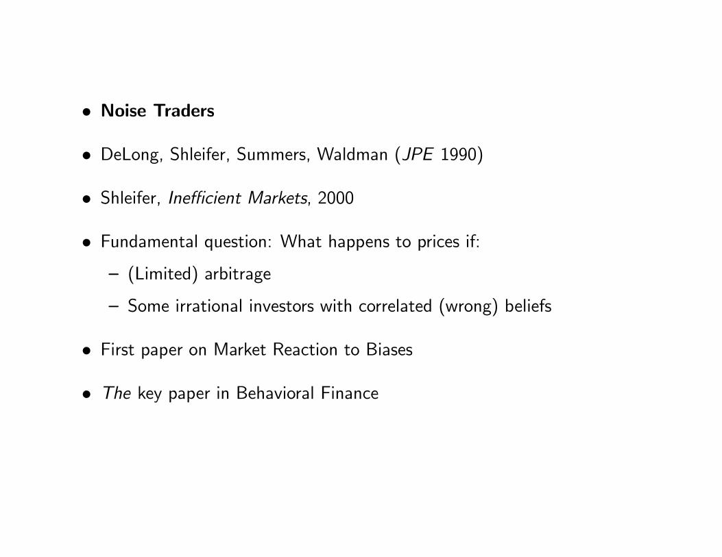
• Noise Traders

• DeLong, Shleifer, Summers, Waldman (JPE 1990)

• Shleifer, Inefficient Markets, 2000

• Fundamental question: What happens to prices if:— (Limited) arbitrage

— Some irrational investors with correlated (wrong) beliefs

• First paper on Market Reaction to Biases

• The key paper in Behavioral Finance

The model assumptions

A1: arbitrageurs risk averse and short horizon

−→ Justification?

* Short-selling constraints

(per-period fee if borrowing cash/securities)

* Evaluation of Fund managers.

* Principal-Agent problem for fund managers.

A2: noise traders (Kyle 1985; Black 1986)

misperceive future expected price at by

∼ N (∗ 2)

misperception correlated across noise traders (∗ 6= 0)

−→ Justification?

* fads and bubbles (Internet stocks, biotechs)

* pseudo-signals (advice broker, financial guru)

* behavioral biases / misperception riskiness

What else?

• noise traders, (1− ) arbitrageurs

• OLG model— Period 1: initial endowment, trade— Period 2: consumption

• Two assets with identical dividend — safe asset: perfectly elastic supply=⇒ price=1 (numeraire)

— unsafe asset: inelastic supply (1 unit)=⇒ price?

• Demand for unsafe asset: and with + = 1

• CARA: () = −−2 ( wealth when old)

[()] =Z ∞∞− −2 · 1q

22· −

122

(−)2

= −Z ∞∞

1q22

· −42+

2+2−222

= −Z ∞∞

1q22

· −(−[22+])2+2−424−2−22

22

= −424+2

2

22

Z ∞∞

1q22

· −(−[22+])2

22

= −422+2 = −2(−2)

¸max [()] y

pos. mon. transf.max − 2

Arbitrageurs:

max( − )(1 + )

+ ([+1] + )

− ( )2 (+1)

Noise traders:

max( − )(1 + )

+ ([+1] + + )

− ( )2 (+1)

(Note: Noise traders know how to factor the effect of future price volatility intotheir calculations of values.)

f.o.c.

Arbitrageurs: [ ]

!= 0

= +[+1]− (1 + )

2 · (+1)

Noise traders: [ ]

!= 0

= +[+1]− (1 + )

2 · (+1)

+

2 · (+1)

Interpretation

• Demand for unsafe asset function of:— (+) expected return ( +[+1]− (1 + ))— (-) risk aversion ()— (-) variance of return ( (+1))

— (+) overestimation of return (noise traders)

• Notice: noise traders hold more risky asset than arb. if 0 (andviceversa)

• Notice: Variance of prices come from noise trader risk. “Price when old”depends on uncertain belief of next periods’ noise traders.

• Impose general equilibrium: + (1− ) = 1 to obtain

1 = +[+1]− (1 + )

2 · (+1)+

2 · (+1)

or

=1

1 + [ +[+1]− 2 · (+1) + ]

• To solve for we need to solve for [+1] = [] and (+1)

[] =1

1 + [ +[]− 2 · (+1) + []]

[] = 1 +−2 · (+1) + ∗

— Rewrite plugging in

= 1− 2 · (+1)

+∗

(1 + )+

1 +

[] = ∙1 +

¸=

2

(1 + )2 () =

2

(1 + )22

— Rewrite

= 1− 222

(1 + )2+∗+ ( − ∗)1 +

— Noise traders affect prices!

— Term 1: Variation in noise trader (mis-)perception

— Term 2: Average misperception of noise traders

— Term 3: Compensation for noise trader risk

• Relative returns of noise traders— Compare returns to noise traders to returns for arbitrageurs :

∆ = − = ( − ) [ + +1 − (1 + )]

(∆|) = −(1 + )2 222

(∆) = ∗ − (1 + )2 (∗)2 + (1 + )2 2

22

— Noise traders hold more risky asset if ∗ 0

— Return of noise traders can be higher if ∗ 0 (and not too positive)

— Noise traders therefore may outperform arbitrageurs if optimistic!

— (Reason is that they are taking more risk)

Welfare

• Sophisticated investors have higher utility

• Noise traders have lower utility than they expect

• Noise traders may have higher returns (if ∗ 0)

• Noise traders do not necessarily disappear over time

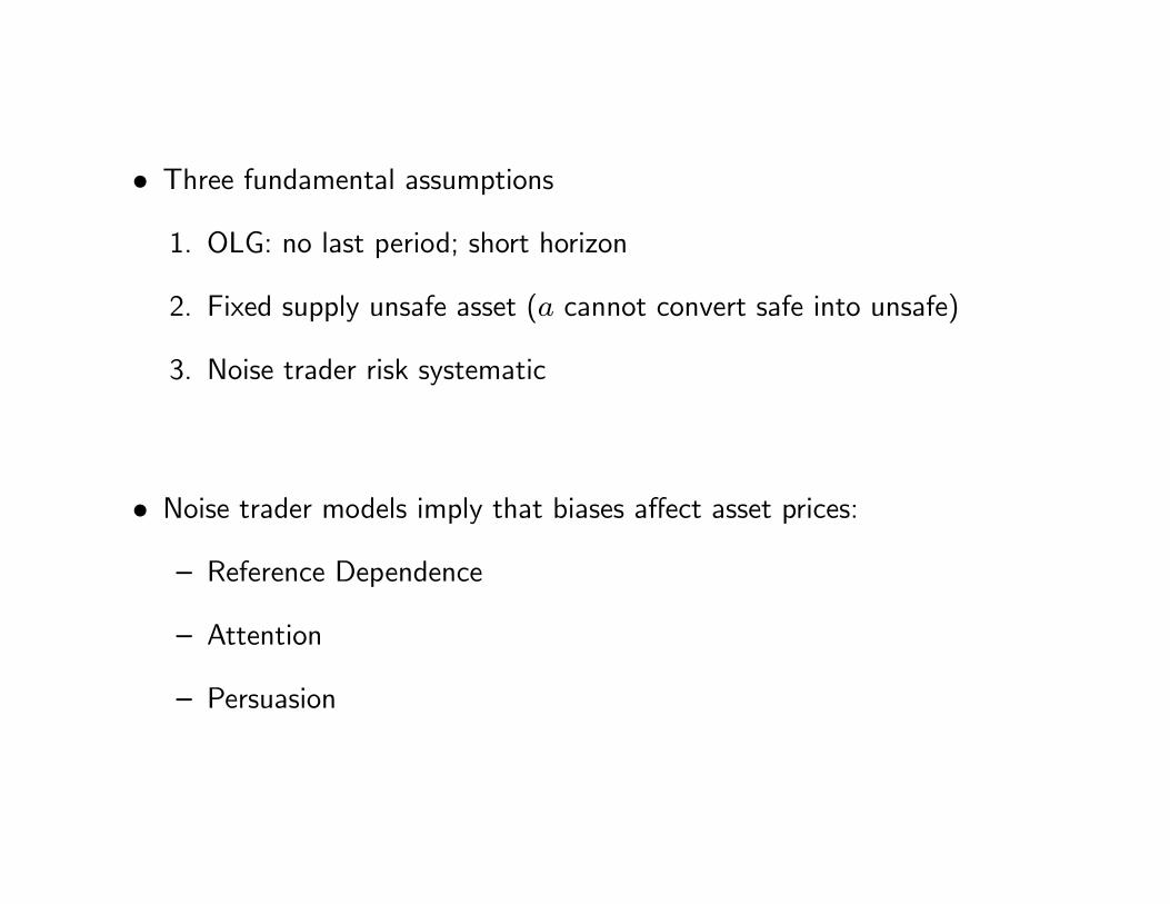
• Three fundamental assumptions1. OLG: no last period; short horizon

2. Fixed supply unsafe asset ( cannot convert safe into unsafe)

3. Noise trader risk systematic

• Noise trader models imply that biases affect asset prices:— Reference Dependence

— Attention

— Persuasion

• Here:— Biased investors

— Non-biased investors

• Behavioral corporate finance:— Investors (biased)

— CEOs (smart)

• Behavioral Industrial Organization:— Consumers (biased)

— Firms (smart)

4 Market Reaction to Biases: Political Economy

• Interaction between:— (Smart) Politicians:

∗ Personal beliefs and party affiliation∗ May pursue voters/consumers welfare maximization∗ BUT also: strong incentives to be reelected

— Voters (with biases):

∗ Low (zero) incentives to vote∗ Limited information through media∗ Likely to display biases

• Behavioral political economy

• Examples of voter biases:

— Effect of candidate order (Ho and Imai)

— Imperfect signal extraction (Wolfers, 2004) — Voters more likely tovote an incumbent if the local economy does well even if... it’s justdue to changes in oil prices

— Susceptible to persuasion (DellaVigna and Kaplan, 2007)

— More? Short memory about past performance?

• Eisensee and Stromberg (2007): Limited attention of voters

• Setting:

— Natural Disasters occurring throughout the World

— US Ambassadors in country can decide to give Aid

— Decision to give Aid affected by

∗ Gravity of disaster

∗ Political returns to Aid decision

• Idea: Returns to aid are lower when American public is distracted by amajor news event

• Main Measure of Major News: median amount of Minutes in Evening TVNews captured by top-3 news items (Vanderbilt Data Set)

• — Dates with largest news pressure

• 5,000 natural Disasters in 143 countries between 1968 and 2002 (CRED)— 20 percent receive USAID from Office of Foreign Disaster Assistance(first agency to provide relief)

— 10 percent covered in major broadcast news— OFDA relief given if (and only if) Ambassador (or chief of Mission) incountry does Disaster Declaration

— Ambassador can allocate up to $50,000 immediately

• EstimateRe = + +

• Below: about the Disaster is instrumented with:— Average News Pressure over 40 days after disaster— Olympics

• — 1st Stage: 2 s.d increase in News Pressure (2.4 extra minutes) decrease

∗ probability of coverage in news by 4 ptg. points (40 percent)∗ probability of relief by 3 ptg. points (15 percent)

• Is there a spurious correlation between instruments and type of disaster?• No correlation with severity of disaster

• OLS and IV Regressions of Reliefs on presence in the News• (Instrumented) availability in the news at the margin has huge effect: Al-most one-on-one effect of being in the news on aid

• Second example: Theory/History paper, Glaeser (2005) on Political Econ-omy of Hatred

• Idea: Hatred has demand side and supply side— Demand side:

∗ Voters are susceptible to hatred (experiments: ultimatum game)∗ Media can mediate hatred

— Supply side:

∗ Politicians maximize chances of reelection∗ Set up a hatred media campaign toward a group for electoral gain∗ In particular, may target non-median voter

• Idea:— Group hatred can occur, but does not tend to occur naturally

— Group hatred can be due to political incentives

— Example 1: African Americans in South, 1865-1970

∗ No hatred before Civil War∗ Conservative politicians foment it to lower demand for redistribution∗ Diffuse stories of violence by Blacks

— Example 2: Hatred of Jews in Europe, 1930s

∗ No hatred before 1920∗ Jews disproportionately left-wing∗ Right-wing Hitler made up Protocol of Elders of Zion

5 Next Lecture

• More Market Response to Biases— Managers: Corporate Decisions

— Welfare Response to Biases

• Methodology of Field Psychology and Economics

• Concluding Remarks