Chapter three

Feeding

3.1 INTRODUCTION

The survival. growth and reproduction of a fish depend on the income of energy and nutrients generated by its feeding activities. Although fishes have a considerable capacity to resist starvation (Love. 1980) and many species normally cease to feed at times during their life cycle (Wootton. 1979). the capacity of individuals to survive such periods depends on their ability to lay down reserves which can be mobilized when feeding ceases. The size of such reserves will reflect feeding success. An ecological analysis of feeding must answer three basic questions: what is eaten. when is it eaten and how much is eaten?

3.2 TROPHIC CATEGORIES IN FISHES

Fishes occupy virtually every possible trophic role. from herbivorous species such as the menhaden. Brevoortia tyrannus. feeding on unicellular algae. to secondary carnivores. for example the pike which eats other fish. amphibians. birds and mammals (Keenleyside. 1979). Some species form part of the decomposer food chain. utilizing detritus or scavenging carcasses. There is even a cichlid that feeds on decomposing hippopotamus faeces! Other unusual methods of obtaining food have also evolved. The archer fish (Toxotidae) can spit out a jet of water to knock terrestrial insects into the water. Angler fish (Lophiiformes) attract prey close with a moveable lure formed by a modific­ation of a ray of the dorsal fin. A general classification of trophic categories is shown in Table 3.1.

Although this classification provides a useful summary of the range of feeding habits. it should not be taken as rigid because many species show great flexibility in their trophic ecology (Keenleyside. 1979; Dill. 1983). Examples of

R. J. Wootton, Ecology of Teleost Fishes© R. J. Wootton 1990

Morphological adaptations

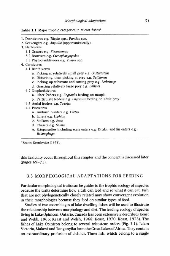
Table 1.1 Major trophic categories in teleost fishes·

1. Detritivores e.g. Tilapia spp .. Puntius spp. 2. Scavengers e.g. Anguilla (opportunistically) 3. Herbivores

3.1 Grazers e.g. Plecostomus 3.2 Browsers e.g. Ctenopharyngodon 3.3 Phytoplanktivores e.g. Tilapia spp.

4. Carnivores 4.1 Benthivores

a. Picking at relatively small prey e.g. Gasterosteus b. Disturbing. then picking at prey e.g. Sufflamen c. Picking up substrate and sorting prey e.g. Lethrinops d. Grasping relatively large prey e.g. Balistes

4.2 Zooplanktivores a. Filter feeders e.g. Engraulis feeding on nauplii b. Particulate feeders e.g. Engraulis feeding on adult prey

4.3 Aerial feeders e.g. Toxotes 4.4 Piscivores

a. Ambush hunters e.g. CoUus b. Lurers e.g. Lophius c. Stalkers e.g. Esox d. Chasers e.g. Salmo e. Ectoparasites including scale eaters e.g. Exodon and fin eaters e.g.

Belanophago.

• Source: Keenleyside (1979).

33

this flexibility occur throughout this chapter and the concept is discussed later (pages 69-71).

3.3 MORPHOLOGICAL ADAPTATIONS FOR FEEDING

Particular morphological traits can be guides to the trophic ecology of a species because the traits determine how a fish can feed and so what it can eat. Fish that are not phylogenetic ally closely related may show convergent evolution in their morphologies because they feed on similar types of food.

Studies of two assemblages of lake-dwelling fishes will be used to illustrate the relationship between morphology and diet. The feeding ecology of species living in Lake Opinicon. Ontario. Canada has been extensively described (Keast and Webb. 1966; Keast and Welsh. 1968; Keast. 1970; Keast. 1978). The fishes of Lake Opinicon belong to several teleostean orders (Fig. 3.1). Lakes Victoria. Malawi and Tanganyika form the Great Lakes of Africa. They contain an extraordinary profusion of cichlids. These fish. which belong to a single

34 Feeding

~ ~ Labidesthes (Atherinidae) Notropis (Cy rinidae)

~ Pimephales (Cyprinidae)

;~:3r;"~ Umbra (Umbridae)

Fundulus (Cyprinodontidae) ~

~~

~~ Pomox is (Centrarchidae) Idalurus (Ictaluridae)

~ ~"~""P":'~d'" ~ Esox (Esocidae)

~ ~

L epomis (Centrarchidae)

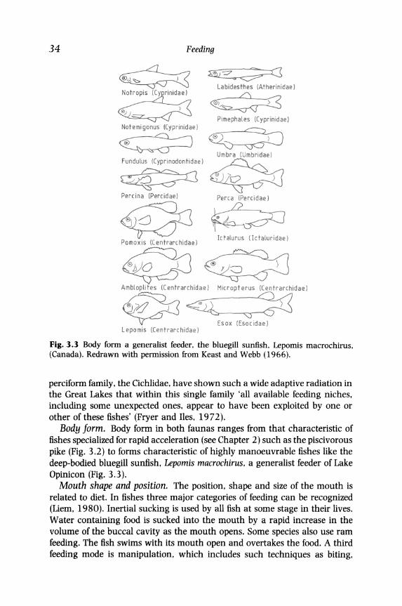
Fig. 3.3 Body form a generalist feeder. the bluegill sunfish. Lepomis macrochirus. (Canada). Redrawn with permission from Keast and Webb (1966).

perciform family. the Cichlidae. have shown such a wide adaptive radiation in the Great Lakes that within this single family 'all available feeding niches. including some unexpected ones. appear to have been exploited by one or other of these fishes' (Fryer and Iles. 1972).

Body form. Body form in both faunas ranges from that characteristic of fishes specialized for rapid acceleration (see Chapter 2) such as the piscivorous pike (Fig. 3.2) to forms characteristic of highly manoeuvrable fishes like the deep-bodied bluegill sunfish. Lepomis macrochirus. a generalist feeder of Lake Opinicon (Fig. 3.3).

Mouth shape and position. The position. shape and size of the mouth is related to diet. In fishes three major categories of feeding can be recognized (Liem. 1980). Inertial sucking is used by all fish at some stage in their lives. Water containing food is sucked into the mouth by a rapid increase in the volume of the buccal cavity as the mouth opens. Some species also use ram feeding. The fish swims with its mouth open and overtakes the food. A third feeding mode is manipulation. which includes such techniques as biting.

Morphological adaptations 35

Esox lucius

Rh amphochro mis long ic eps

Fig. 3.2 Body form in two unrelated piscivores. pike. Esox lucius. from 1. Opinicon and a cichlid. Rhamphochromis longiceps. from L. Malawi. Redrawn with permission from Keast and Webb (1966) and from Fryer and Iles (1972).

Fig. 3.3 Body form of a generalist feeder. the bluegill sunfish. Lepomis macrochirus. (adult length c .• 180mm). Redrawn and Simplified with permission from Scott and Crossman (1979).

scraping. rasping. gripping and clipping. The ability to protrude the jaw is common in the more evolutionarily advanced fishes (Fig. 3.4). The advan­tages of this in feeding have yet to be fully defined (Motta. 1984). Protrusion may momentarily but crucially increase the rate of approach of the predator to its prey; it may increase the distance from which a prey may be sucked; it may decrease the rotation of the lower jaw required to close the mouth once the prey is captured (Motta. 1984; Osseo 1985). The ability to protrude the jaw may also confer an advantage in specific circumstances such as obtaining benthic prey or food from otherwise inaccessible places (Alexander. 1967; Osseo 1985),

Fishes feeding at the surface or in the middle ofthe water column frequently have a dorso-terminal or terminal mouth. Two examples from Lake Opinicon are the golden shiner. Notemigonus chrysoleucas. a cyprinid with a protrusible

36 Feeding

Clospd mouth

LO I'i ER JA',. PREMAX ILL A

Fig. 3.4 Schematic diagram of jaw protrusion in a cichlid. Arrows show direction of movement of various bones; position of ligaments shown by lines. Redrawn with permission from Fryer and Iles (1972).

jaw (Fig. 3.5). and the brook silverside. Labidesthes sicculus. an atherinid. Pelagic. zooplanktivorous cichlids of Lake Malawi have a terminal mouth which forms a protrusible tube (Fig. 3.5). In Lake Opinicon. the bluegill sunfish is a generalized feeder. eating zooplankton. insect larvae. crustaceans. molluscs and fish fry. It has a narrow. terminal mouth which is tubular when protruded (Fig. 3.5). The major piscivores of Lake Opinicon are the pike and the largemouth bass. Micropterus salmoides. a centrarchid (Fig. 3.1). These have a wide mouth aperture and a strong jaw. In the pike there is also a noticeable flattening of the head (Fig. 3.2). Piscivorous cichlids of the African Great Lakes also have mouths with a large gape and their head shape gives some species a pike-like appearance (Fig. 3.2). The bluntnose minnow. Pimephales notatus. of Lake Opinicon feeds on organic detritus and inverte­brates from the substrate. Its mouth is ventro-terminal. A bottom-feeding cichlid from Lake Malawi. Lethrinops furcifer. has a highly protractile mouth which it uses to vacuum-clean through the substrate to collect chironomid larvae (Fig. 3.6).

Marginal and pharyngeal teeth. Fish may carry teeth on the tongue. the marginal bones of the jaw. the palatal bones and the pharyngeal bones. The marginal teeth of the fishes of Lake Opinicon. with the exception of the cyprinids which lack them. are relatively unspecialized cones. straight or recurved. In the pike. the marginal and palatal bones are angled so that the prey can only move down the throat. In contrast. the African Great Lakes cichlids show a diversity of marginal teeth (Fig. 3.7).

The pharyngeal bones in the throat are well developed in the African Great

,~ No temigonus

Haplochromis cyaneus

Lepomis

Fig. 3.5 Some examples of jaw protrusion from L. Opinicon (Notemigonus and Lepomis) and L. Victoria (Haplochromis cyaneus). Redrawn with permission from Keast and Webb (1966) and from Fryer and Iles (1972).

Fig. 3.6 Feeding of Lethrinopsfurcifer, a sand-digging cichlid from L. Malawi. showing 'vacuum cleaning' of substrate. Redrawn with permission from Fryer and Iles (1972).

l:b

EMPL

OYER

S OF

SU

BTER

FUG

E F

ig.

3.7

Rel

atio

nshi

p be

twee

n sh

ape

of m

argi

nal

and

phar

ynge

al t

eeth

and

die

t fo

r ci

chli

ds

from

L.

M

alaw

i. (T

roph

ic

stat

us

of

'eye

bite

r' un

cert

ain.

) R

edra

wn

and

sim

plif

ied

wit

h pe

rmis

sion

fro

m F

ryer

and

Ile

s (1

972)

.

Morphological adaptations 39

Lakes cichlids (Fryer and nes. 1972; Liem. 1973; Greenwood. 1984). There are two sets of bones. one in the roof of the throat and the other on the floor. Any food passing through to the oesophagus must pass between the upper and lower sets as though passing between a pair of millstones (Fig. 3.8). The surfaces of the bones carry teeth whose shape correlates with diet. Examples of the pharyngeal dentition of some cichlids are shown in Fig. 3.7. The convergent evolution in tooth shape in. for example. those cichlids that feed by crushing molluscs is striking. In Lake Opinicon. the pumpkinseed sunfish. Lepomis gibbosus. feeds on molluscs and isopods. Its stout. flattened pharyngeal teeth act as a grinding mechanism. The bluegill sunfish. which feeds on a wide range of small invertebrates. has the surface of its pharyngeal bones covered with fine. needle-like teeth (Keast. 1978).

Gill rakers. Rakers are forward-directed projections from the inner margins ofthe gill arches. Their shape and abundance are related to diet. Fish that feed on small food particles usually have numerous long. fine rakers (Fig. 3.9) whereas fish feeding on large particles have fewer. shorter. blunter rakers. The brook silverside of Lake Opinicon has abundant long rakers. whereas the more

~UPPE~ PHARYNGEAL

_~BONE

-- .... , ( + ~ OESOPHAGUS

/~····+·"L~O-W::RYNGEAL BONE

Fig. 3.8 Upper: three examples of pharyngeal bones from African Great Lake cichlids showing inter-specific variation in form of pharyngeal teeth. Lower: the pharyngeal mill of the cichlids. Solid arrows show direction of movement of pharyngeal bones; broken arrows show food path. Redrawn with permission from Fryer and lies (1972).

40

GILL FILAMENT

Feeding

GILL ARCH

Fig. 3.9 Gill arch showing arrangement of gill rakers in planktivorous fish. Modified after Zaret (1980).

generalist feeders. the sunfish. have rakers that are short and few in number (Keast. 1978).

In fishes like the menhaden that filter-feed on phytoplankton or small zooplankton the gill rakers probably sieve the food particles from the respiratory current (Friedland. 1985). The detailed mechanism of the sieving action and the collection of food is not fully understood (Lauder. 1983). In those zooplanktivores that feed by snapping up their prey. such as the lake whitefish. Coregonus cIupeaformis. the size of prey ingested is not a simple function of the sieve mesh of the rakers (Seghers. 1974a; Zaret. 1980). The

V> uJ

u.. o 0: uJ a:J L => Z

16

~~--------------------~r--

~~~~+-~~~~~~~ 80

CAN AL

Fig. 3.10 Relationship between relative gut length and diet in a sample of African Great Lakes Cichlids. Top. carnivores; middle. omnivores; bottom. herbivores. Redrawn with permission from Fryer and lies (1972).

Diet composition 41

precise role during feeding of the rakers in these and other particulate-feeding fishes remains unclear (O'Brien. 1987).

Alimentary canal. There is a correlation between the diet and the gut length relative to body length (Kapoor et a!.. 1975). This is illustrated by the relative gut lengths of carnivorous. omnivorous and herbivorous cichlids from Lake Tanganyika (Fig. 3.10). Fish consuming high-quality food can process it with a gut that is shorter than their total length. Fish whose diet includes a high proportion of material that resists digestion. such as cellulose or lignin have guts that are several times longer than their body length. The Indian cyprinid. Labeo horie, feeds on detritus and has a gut length that is 15 to 21 times its body length (Bond. 1979).

A statistical analysis ofthe relationship between gut length and body length for fishes from a freshwater creek in South Carolina shows that for individual species. the relationship between gut length (GL) and total length (TL) is described by the allometric form: GL = aTLb. where a and b are constants. For several species. the exponent b is significantly greater than unity, indicating that the relative gut length increases with an increase in fish length (Ribble and Smith. 1983). The functional implications ofthis allometric growth ofthe gut are obscure.

Carnivorous fishes usually have a large stomach. which in some species has pyloric caeca associated with it. These are blind-ending tubes that arise as outgrowths ofthe pyloric region ofthe gut. In herbivorous fishes. the stomach is often small or absent. In some groups of fishes, including the widely distributed and abundant Cyprinidae. a specialized stomach is absent irrespec­tive of diet.

3.4 DIET COMPOSITION

Although morphology can provide circumstantial evidence ofthe diet of a fish. the inferences must be confirmed by more direct evidence of what is eaten.

Describing dietary composition

A description of the composition of the diet should indicate the relative importance of the items eaten. The flexibility of feeding habits can make even this starting point difficult to achieve. for example the threes pine stickleback. Gasterosteus aculeatus. in a small Welsh reservoir eats about 20 different categories of food (Allen and Wootton, 1984). Diet can rarely be studied by directly observing feeding behaviour and identifying what is eaten. Usually the diet is sampled by extracting the stomach contents, Mher by killing the fish and dissecting out the stomach or by flushing out the stomach. Several methods are used to provide a quantitative description of such samples (Hynes, 1950: Windell. 1971: Hyslop. 1980); probably no one method is entirely satisfactory.

42 Feeding

The simplest method estimates the frequency of occurrence in stomachs. After identification of the food categories present. the number of stomachs in which a given category is found is expressed as a percentage of the total number of stomachs sampled. This method only provides information on the presence or absence of categories and not on their relative numbers or bulk. In the numerical method. the number of items in each food category is counted in all stomachs in the sample. The importance of a category is then usually estimated by expressing the number of items in that category as a percentage of the total number of items counted in all the stomachs. This method emphasizes the importance of small and numerous items such as zooplankton. It cannot be used when the diet contains significant proportions of plant material or detritus. categories which do not include discrete. individual prey. The volumetric and gravimetric techniques emphasize the bulk of the food categories. In the former. the volume of each category in each stomach is estimated. In the latter. the weight of each category is measured. In both methods. the relative importance of a food category can be expressed as a percentage of the total volume or weight of all the categories present in the samples. The points method is essentially a modification of the volumetric method that is quicker to use. The investigator allocates points to each food category in proportion to its contribution to the total volume of the stomach contents. The allocation of points is subjective for it is based on a visual assessment of contribution. This subjectivity of the method can be partially reduced by correcting the points score for the degree of fullness of the stomach (Hyslop. 1980; Allen and Wootton. 1984).

Any of these methods provides a general picture of the composition of the diet. and frequently one that is similar to that provided by the other methods (Hynes. 1950; Pollard. 1973). A fuller picture can be obtained by using the numerical method together with one of the three methods that emphasize the contribution to the volume or weight of the food consumed (Hyslop. 1980). Even then the statistical analysis of such data presents major problems. There may be many food categories in the diet. some of which are present only in small amounts. Fish sampled at the same time and place may have stomach contents that are very different from each other. Some food categories are quickly digested and so difficult to detect. Other categories. for example insect larvae or crustaceans with chitinous exoskeletons. remain identifiable over longer periods of time. The difficulties of rigorously analysing quantitative data obtained by the analysis of stomach contents have yet to be satisfactorily resolved (Crow. 1982).

Measurement 0/ diet selectivity in natural populations

The diet will reflect what food is available in the environment. A fish can be regarded as a sampling device with the contents of its gut representing a sample of what is available. Does a fish take food items strictly in the proportions in which they occur in the environment or does it show some

Diet composition 43

selectivity? Several methods for measuring such selectivity have been developed. An early example is the index of electivity (I vlev. 1961) defined as:

E = (rj - p)/(r j + p)

where E is the index of electivity. rj is the relative abundance of prey category i in the gut. and Pj is the relative abundance of prey category i in the environment. The index can take values between - 1 and + 1. with negative values indicating avoidance or inaccessibility of prey category i. and positive values active selection. A value of zero indicates random selection. Although commonly used. the index of electivity has serious faults (Strauss. 1979; Lechowicz. 1982; Chesson. 1983). Its value depends not only on the behaviour of the forager but on the numbers of each food type present. This usually precludes comparing values for the index obtained at different sites or at different times of the year.

Chesson (1983) suggests a measure of preference for a food item i. aj • which is defined by the relationship:

Pi = ap j! f api i~l

where P j is the probability that the next food item consumed is of type i. ni is the number of type i available and m is the total number of types. Each aj can be interpreted as the proportion ofthe diet which could consist oftype i if all food types were present in equal numbers in the environment. Table 3.2 gives the formulae for calculating aj under different conditions.

An alternatlve approach to the use of indices is the use of statistical techniques to compre the composition of the diet with what is available in the environment. In their study of predation of the alewife. Alosa pseudoharengus. on zooplankton. Kohler and Ney (1982) use a nonparametric statistical test to compare the rank order of prey in the diet with their rank order in the environment. MacDonald and Green (1986) use a multivariate parametric analysis to identify prey selection by an assemblage of benthic-feeding fishes including cod. winter flounder and American plaice. Hippoglossoides plates­soidesoides. off the coast of New Brunswick (Canada). Their technique. called canonical analysis. allows the faunal composition of benthic samples to be compared statistically with the faunal composition of the diet of each species.

Both the indices and the statistical techniques assume that the gut samples and habitat samples accurately reflect the relative abundance of prey consumed and in the environment respectively (Kohler and Ney. 1982). A weakness of indices or statistical analyses of selection is that they give no indication of the mechanisms responsible for any selection identified. They are only guides for identifying situations in which diet selection may be taking place and so for stimulating studies which uncover the processes that result in the selection.

44 Feeding

Table 3.2 Formulae for calculating preference for prey item i, aj' in Chesson's (1983) index of prey preference*

1. No food depletion, nj assumed constant:

(r.jn.) aj = m I I , i = 1, .... , m

L (r;ln;)

2. Food depletion, nj not assumed constant:

a·= I m

loge( (nj(O) - r;)/nj(O))

3. Order of selection of items by consumer known, but only first prey item taken is recorded:

a. = kjln j I m

Where: aj = preference for prey type i nj = number of items of type i present in the environment nj(O) = number of items of type i present in the environment at beginning of

foraging bout rj = number of items of type i in consumer's diet kj = number of consumers whose first food items was of type i

m

K = number of consumers. i.e. L kj = K ;=1

m = number of types in the environment

'Source: Chesson (1983).

Factors that determine prey selection For an item to appear in the diet of a fish it has to be detected, approached, selected, manipulated and digested (Fig. 3.11). Most studies on prey detection and acceptance by fishes use species that detect their prey visually and feed on living prey such as zooplankton (Lazzaro, 1987; O'Brien, 1987), benthic invertebrates or fish. The factors that determine the diet composition of species that rely on non-visual cues to find food, or of detritivores and herbivores generally receive less attention. Given the importance of herbivorous and detritivorous cyprinids and cichlids to aquaculture in developing countries such as India and China this will change.

Prey availability. For prey to appear in the diet of a fish they must be available and accessible given the constraints of the morphology and sensory

Diet composition 45

DETECT • IGNORE

~ APPROACH --AVOID

~ SELECT ~REJECT

~ MANIPULATE -EJECT

~ INGEST

Fig. 3.11 Events in a feeding sequence.

capacities of the fish. This is illustrated by an experiment on rainbow trout. Salmo gairdneri. The trout hunted for amphipods placed at different densities on the bottom of an aquarium. The substrate was changed by placing different sorts of litter on the bottom providing greater or lesser concealment to the amphipods. Although the number of prey attacked increased linearly with an increase in their density. the proportion of prey attacked at a given density decreased with an increase in the concealment provided by the litter (Fig. 3.12) (Ware. 1972).

A field study demonstrates this importance of refuges from predation for the prey. In Marion Lake in British Columbia. Canada. even under favouraole conditions less than 30% of the amphipod population are at the substrate/water interface and thus exposed to predation by rainbow trout. At low temperatures in winter. the vulnerable portion of the amphipod popul-

200 • •

0 150 0

0 a u.J a:: => f-0.. a <{

100 w • a:: • u.J 0 en 0 ::E • => a z

50 a

ct • a • -a

150 200

INITIAL DENSI TY

Fig. 3.12 Effect of litter on capture success of rainbow trout. Salmo gairdneri. feeding on amphipods (HyaIIela) . •• no litter: 0 . large litter covering c. 6% of bottom: 0 . large litter covering c. 15% of bottom: •. smaller litter covering 100% of bottom. Redrawn with permiSSion from Ware (1972).

46 Feeding

ation falls to as low as 2%. the remaining 98% being concealed within the substrate (Ware. 1973). Ecological studies which seek to analyse the availability of prey to a predatory fish have to estimate not only the absolute abundance of the prey. but also that proportion of the prey population that is at risk of predation.

Prey and predator characteristics in prey selection. Selection may occur because of differences in the detectability of the potential prey. This form of selection is related to the sensory capacities of the predator and the ability of the prey to avoid detection. The predator may detect the prey then fail to capture it because of morphological or behavioural constraints. The predator may detect the prey and be able to ingest it. but reject it in favour of another prey.

For fish predators hunting by sight. the important visual characteristics of the prey are size. contrast with the background and movement. Other relevant characteristics may be shape. colour and oddity (Wootton. 1984a).

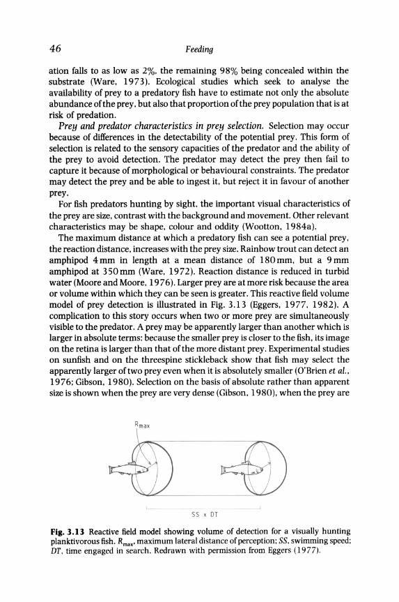
The maximum distance at which a predatory fish can see a potential prey. the reaction distance. increases with the prey size. Rainbow trout can detect an amphipod 4 mm in length at a mean distance of 180 mm. but a 9 mm amphipod at 350mm (Ware. 1972). Reaction distance is reduced in turbid water (Moore and Moore. 1976). Larger prey are at more risk because the area or volume within which they can be seen is greater. This reactive field volume model of prey detection is illustrated in Fig. 3.13 (Eggers. 1977. 1982). A complication to this story occurs when two or more prey are Simultaneously visible to the predator. A prey may be apparently larger than another which is larger in absolute terms: because the smaller prey is closer to the fish. its image on the retina is larger than that of the more distant prey. Experimental studies on sunfish and on the threespine stickleback show that fish may select the apparently larger oftwo prey even when it is absolutely smaller (O'Brien et aI .• 1976; Gibson. 1980). Selection on the basis of absolute rather than apparent size is shown when the prey are very dense (Gibson. 1980). when the prey are

Rmax

55 x DT

Fig. 3.13 Reactive field model showing volume of detection for a visually hunting planktivorous fish. Rmax' maximum lateral distance of perception; SS. swimming speed; DT. time engaged in search. Redrawn with permission from Eggers (1977).

Diet composition 47

close to the fish. or when the apparently larger prey is not directly in front of the fish but off to one side (O'Brien et aI .. 1985; O·Brien. 1987). For the apparent size model to operate. prey must be sufficiently abundant for more than one to be visible simultaneously. At low prey densities. the reactive field volume model is appropriate.

The consequences for prey populations of selection by size are shown by the effects of the introduction of planktivorous fishes into waters that previously lacked them (Zaret. 1980; O·Brien. 1987). Sporley Lake in Michigan (USA) was cleared offish by poisoning. allowed to recover and stocked with rainbow trout; fathead minnows. PimephaIes promeIas. and smelt were also introduced (Galbraith. 1967). As the numbers of fish increased. the composition of the zooplankton assemblage changed. There was reduction in the mean size ofthe mature Daphnia. a replacement of larger by smaller daphnid species. and a subsequent replacement of daphnids by smaller cladocerans such as Bosmina. Such changes in the size spectrum of prey species can have effects on the fish species that can coexist in the same habitat (see discussions in Chapters 9 and 12).

Reaction distance increases with an increase in visual contrast between the prey and the background (Ware. 1971). An elegant demonstration of the importance of contrast is provided by Zaret (1972. 1980). The freshwater planktivore Melaniris chagresi. an atherinid from Central America. eats the cladoceran Ceriodaphnia cornuta. The fish preys preferentially on one of the two morphs of the cladoceran present in Gatlin Lake. Panama. There is no difference in body size between the two morphs. but the morph which is eaten more has the larger black compound eye. Feeding India ink particles to the morph with the less conspicuous eye makes it more conspicuous than the morph with the larger eye. and the fish switch to feeding on the morph containing the ink.

As light levels decline. the contrast between prey and background will usually decline. Visually hunting fish show a sigmoidal relationship between light intensity and feeding intensity. As light levels increase from total darkness. the feeding intensity shows little change until a threshold level of light intensity is reached. Feeding intensity then increases rapidly to a maximum with any further increase in light intensity (Dabrowski. 1982a). Larval roach. Rutilus rutilus. continue to feed on zooplankton at extremely low light intensities. but this ability may depend on the lateral line system rather than sight (Dabrowski. 1982b).

Movement is the third important prey characteristic. The reaction distance of rainbow trout feeding on pieces of blanched liver is significantly greater when the liver is kept in motion (Ware. 1973). Mysids are important in the diet of the littoral fifteens pine stickleback. Spinachia spinachia. The stickleback prefers moving mysids to stationary ones unless the prey are moving slowly. The frequency of attempted or completed feeding responses by the stickleback increases with the speed of movement of the mysid up to a speed of about

48 Feeding

30 mm s - I. but then declines with a further increase (Kislalioglu and Gibson. 1976a).

Size. contrast and movement are in most situations the most important prey characteristics for a predator hunting by sight. But other factors can become relevant. When attacking a swarm of Daphnia. threespine sticklebacks will turn their attention to Daphnia that differ in colour from others (Ohguchi. 1981). Prey that are behaving oddly. perhaps because of injury or deformity may also be more at risk (Curio. 1976).

Having detected a potential prey. the predator has to pursue. capture and ingest it. Some fish predators chase their prey. whereas others ambush them. Capture success can depend on the body form and mode of locomotion of the predator (see Chapter 2). Tunas. which are specialized for cruising. may catch only 10-15% of the fish they strike at. whereas the pike. a specialist ambush piscivore. can catch 70-80% of their intended prey. Generalist predators such as trout and perch (Perea) have success rates of about 40-50% (Webb. 1984b). The ability of prey to avoid the tactics of the predator can also be important in determining diet composition. Zooplanktivorous fish often take cladocerans in preference to copepods perhaps because the copepods have a more erratic mode of swimming and are less easy to capture (Zaret. 1980; O·Brien. 1987).

After capture. prey palatability can be a factor. Threespine sticklebacks used to feeding on Tubifex worms nevertheless show a strong preference for enchytraeid worms when these are also made available. The presence of the enchytraeid worms causes a significant reduction in the risk of predation to the Tubifex (Beukema. 1968).

Dietary composition will also reflect morphological constraints including mouth size and the spacing of the gill rakers. Coho salmon fry. Oncorhynchus kisutch. 40-80 mm in length show a decrease in the proportion of the prey they ingest as prey width increases from 2 mm to 6 mm (Fig. 3.14). For a coho of a given length the proportion of prey ingested decreases rapidly with an increase in prey width above a critical width. This critical width is greater for

UJ 1 ·0 a:: => I-"-<t w

"-0

>- o 5 !:: =! en <t en 0 a::

0 "-0 04 0·6 0·8 4

PREY WIDT H (mm)

Fig. 3.14 Model of effect of prey width on probability of successful capture by fish of three lengths. 40. 60 and 80 mm. Model is based on data from juvenile coho salmon. Oncorhynchus kisutch. Redrawn with permission from Dunbrack and Dill (1983).

Diet composition 49

the bigger fry because their gape increases (Dunbrack and Dill, 1983), Fry of the Atlantic salmon show a similar effect of prey size on the chances of rejection (Wankowski, 1979). For both species of salmon fry, the probability of ingestion also decreases when prey are below a critical width. This lower limit may be set by the spacing of the gill rakers or the difficulty of seeing small prey. A model of prey selection by coho fry feeding on drifting invertebrates, based on the relationship between prey size and the probability of ingestion (Fig. 3.14) gives a good prediction of the diet of coho in a stream (Dunbrack and Dill, 1983).

As prey size increases, the predator has to pay an increasing cost in the time taken to handle the prey. Experiments on species of sunfish and on the fifteenspine stickleback show that as the size of the prey increases relative to the predator's mouth size, the handling time increases slowly at first, but then sharply as the prey size approaches the gape size (Fig. 3.15) (Werner, 1974; Kislalioglu and Gibson, 1976b). Handling time also increases as the fish become satiated (Ware, 1972; Werner, 1974; Kislalioglu and Gibson, 1976b). This increase in handling time with prey size is important for two reasons. Firstly, there is not an infinite 'supply of time for foraging, and time spent handling a prey cannot be spent seeking and pursuing other prey. Secondly, handling time is a factor that determines the profitability of a prey to a predator, a point taken up again on page 51.

Prey digestibility. Even after ingestion, some prey may not contribute to the diet because they are not successfully digested. Ostracods are micro-

\:J ~ -' Cl

300

250

200

z 100 « OJ:

50

00 02 0·4 0·6 o·a 10

TP/MS

Fig. 3.15 Relationship between handling time and prey thickness relative to mouth diameter (TP /MS) for fifteenspine sticklebacks, Spinachia spinachia, feeding on mysids. Redrawn with permission from Kislalioglu and Gibson (197 6b).

50 Feeding

crustaceans that are protected by a carapace which encloses the whole body. Some ostracods are able to pass through the alimentary canal of a fish and emerge alive (Victor et aI., 1979). Herbivorous fishes do not have rumens in which digestion of cellulose and lignin is achieved by a microbial flora. Instead they rely on breaking open plant cell walls mechanically or chemically. Herbivorous cyprinids rely on the mechanical action of their pharyngeal teeth (Sillah, 1981), but herbivorous cichlids can achieve highly acidic conditions in their stomach (Moriarty and Moriarty, 1973). However, some intact plant cells are defecated.

Effects of experience of the predator. Fish may have to learn that an object is edible and this may cause a time-lag between the appearance of a prey item and its effective exploitation by the fish (Werner et aI., 1981). Rainbow trout exposed to novel prey, for example blanched pieces ofliver, take several days to accept the food (Ware, 1971). Most trout do not approach it until the fourth day of presentation and take two additional days to complete the development of the feeding response. Even then, the feeding performance of the trout improves further. The distance from which the trout approach the food increases with experience to about twice that at which na'ive fish react. The trout show a reduction in their reaction distance back to the level of naive fish when the liver is dyed black, although the distance improves with experience suggesting that the fish have to learn the prey characteristics (Ware, 1971).

The pattern of movement of a foraging fish is influenced by experience. Threespine sticklebacks hunting for Tubifex in a maze consisting of linked hexagonal cells progressively modify their search paths with experience of the maze (Beukema, 1968). This change in behaviour increases the effectiveness with which they search the maze and encounter prey. An encounter with a Tubifex worm also influences a stickleback's behaviour. If the worm is eaten, the stickleback tends to stay in the area of discovery, increasing its intensity of searching and its frequency of approaching the substrate. This change in behaviour leads to area-restricted searching. If the worm is rejected the fish tends to move away and initially decrease the intensity of its searching, leading to area-avoided searching (Thomas, 1974, 1977). Rainbow trout will switch from searching behaviour to undirected swimming when their rate of prey capture falls below about 0.06 captures S-1 (Ware, 1972).

The problems of observing fish foraging in the field make it difficult to assess the importance of these experimental effects on diet composition. Fish from the same population sampled at the same time can have significant differences in their diet (Bryan and Larkin, 1972). These may reflect differences in the experiences of the fish as they forage. Rainbow trout can be trained to show a preference for a familiar food, but this bias is weak and may not be an important factor in determining food selection under natural conditions (Bryan, 1973). However, the effects of prior experience may cause difficulties when hatchery-reared fish are stocked into natural waters, because the fish

Diet composition 51

have to change from feeding on artificial. usually pelleted food to feeding on natural prey.

Optimal foraging

Models that seek to predict dietary composition from a knowledge of the sensory, morphological and behavioural characteristics of the forager are called mechanistic models because the mechanisms which lead to the selection of prey are defined. The reactive field model and apparent size model used to predict the dietary composition of planktivores (see pages 46-47) provide examples. A complementary set of functional models of foraging behaviour seek to predict the diet composition by assuming that the action of natural selection on the physiology, morphology and behaviour involved in feeding maximizes the Darwinian fitness of the forager. Because of the difficulties of directly measuring the effect of foraging behaviour on fitness, it is usually assumed that the forager attempts to maximize the rate of food consumption per unit time. Most models assume that the net rate of food consumption is maximized, where net food consumption is measured as the gross energy content of the food less the energy cost of acquiring it. These optimal foraging models do not seek to describe the mechanisms by which the forager achieves this maximization, but only to predict outcomes such as what is eaten and where is searched for prey (Pyke, 1984; Krebs and Stephens, 1986). The application of optimal foraging models to fishes is reviewed by' Townsend and Winfield (1985 and Hart (1986).

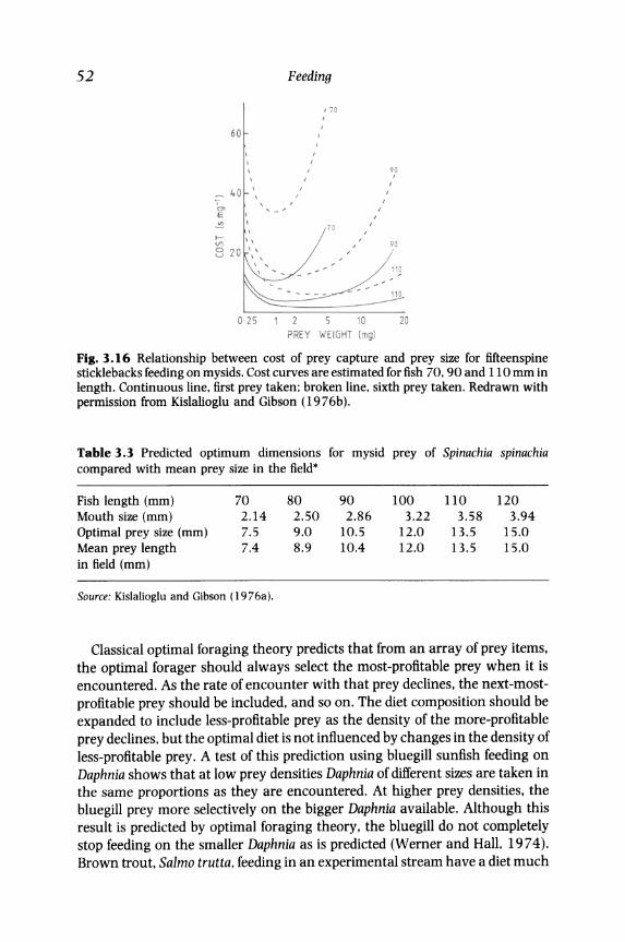
Prey selection. If the net or gross energy intake per unit time is to be maximized, then the most profitable prey will be those for which the cost of prey capture is minimized. One measure of this cost is the time taken to handle the prey (h) divided by the weight (or better the energy content) of the prey (r), that is h/r. This measure of cost can be further modified to incorporate the time costs of searching and capture. The relationship between cost, prey size and predator size has been estimated for bluegill sunfish (Werner, 1974) and the fifteenspine stickleback (Kislalioglu and Gibson, 19 76b). In both species, the cost first decreases with an increase in prey size because the handling time increases only slowly with an increase in prey size (Fig. 3.15). Then cost increases as the handling time increases sharply with a further increase in prey size until the prey become too large to be handled by the fish. This U-shaped curve means that for a predator of a given size, there is a prey size that minimizes cost (Fig. 3.16). Larger predators have a bigger optimal prey size and a wider range of prey sizes that impose costs close to the minimum (Fig. 3.16). Such estimates of the costs (or their inverse, profitabilities) of the prey can then be used to predict the optimal composition of the diet. For the fifteenspine stickleback there is a high correlation between the predicted optimal prey size and the mean prey size taken by fish in the wild (Table 3.3). There is also evidence that the range of prey sizes taken increases with an increase in the size of the fish (Kislalioglu and Gibson, 1976b).

52

60

7' 40 '. CJl E

Feeding

, 70

70

0·25 1 2 10 PREY WEIGHT (mg)

90 ,

, ,

90

1 ~ 9

110

20

Fig. 3.16 Relationship between cost of prey capture and prey size for fifteenspine sticklebacks feeding on mysids. Cost curves are estimated for fish 70, 90 and 110 mm in length. Continuous line, first prey taken: broken line, sixth prey taken. Redrawn with permission from Kislalioglu and Gibson (19 76b).

Table 3.3 Predicted optimum dimensions for mysid prey of Spinachia spinachia compared with mean prey size in the field·

Fish length (mm) 70 80 90 100 110 120 Mouth size (mm) 2.14 2.50 2.86 3.22 3.58 3.94 Optimal prey size (mm) 7.5 9.0 10.5 12.0 13.5 15.0 Mean prey length 7.4 8.9 10.4 12.0 13.5 15.0 in field (mm)

Source: Kislalioglu and Gibson (1976a).

Classical optimal foraging theory predicts that from an array of prey items, the optimal forager should always select the most-profitable prey when it is encountered. As the rate of encounter with that prey declines, the next-most­profitable prey should be included, and so on. The diet composition should be expanded to include less-profitable prey as the density of the more-profitable prey declines, but the optimal diet is not influenced by changes in the density of less-profitable prey. A test of this prediction using bluegill sunfish feeding on Daphnia shows that at low prey densities Daphnia of different sizes are taken in the same proportions as they are encountered. At higher prey densities, the bluegill prey more selectively on the bigger Daphnia available. Although this result is predicted by optimal foraging theory, the bluegill do not completely stop feeding on the smaller Daphnia as is predicted (Werner and Hall, 1974). Brown trout, Salmo trutta, feeding in an experimental stream have a diet much

Diet composition 53

closer to the predicted optimal diet than to a random selection of the prey supplied, but it does not reach the predicted composition (Ringler, 1979). The trout improve their feeding performance over a period of days showing an effect of experience. In contrast, perch, Percafluviatilis, preying on Daphnia or Chaoborus larvae either separately or together feed about equally on both types of prey when these are together. The profitabilities of the two prey types when avilable separately suggest that an optimally foraging perch should select only Chaoborus from the mixture (Persson, 1985).

The apparent failure of fish to choose a predicted optimal diet may indicate that the variable that is assumed to be maximized has been incorrectly identified. The fish is maximizing something else. Fish may lack the inform­ation required to make an optimal choice. Another possible explanation is that there is a lack of suitable genetic variation in the population so an optimal solution cannot evolve through natural selection. One of the great advantages of a good model is that deviations from its predicted outcomes can help to identify important components of the process being modelled.

Optimal foraging theory is used with conspicuous success by Werner and his co-workers as a guide to organizing empirical evidence and suggesting future research in a study of the interrelationships between sunfishes in North American lakes (Werner and Mittelbach, 1981). This programme has used a powerful combination of theoretical, experimental and field studies in an exemplary way. The results are treated in more detail in Chapters 8 and 9 which discuss interspecific interactions, but an example of the approach applied to a single species, the bluegill sunfish, is relevant here (Mittelbach, 1981a, b; Werner and Mittelbach, 1981). An expression for the net profitability of prey to the sunfish is derived in terms of net energy intake. An important variable is the rate of encounter with prey of a given size in a given habitat. Laboratory experiments in which bluegill are allowed to hunt for prey in three different types of habitat provide data which allow encounter rates to be predicted from a knowledge of prey size, prey density and fish size (Fig. 3.17). The abundance and size spectrum of prey available in a small lake are estimated and this information is used to predict the optimal diet for bluegill of different lengths. These predicted optimal diets are then compared with the diets observed in the lake. There is a striking correspondence between the predicted and observed diets, although the correspondence between the observed diet and the size spectrum of prey available in the habitats sampled is weak (Fig. 3.18). Optimal foraging theory is used successfully to predict the pattern of selective predation by bluegills.

Classical optimal foraging theory assumes that the forager has perfect knowledge of the profitabilities of different prey but does not specify how such information is achieved. The rules which foragers use to approach an optimal diet may depend on a learning process or on relatively simple rules of thumb such as always select the largest prey visible (Krebs and Stephens, 1986). The importance of such rules is now an active field of research. A second weakness

20 I11III

ii u z ....

~ PREY LENGTH

~

PREY DENSITY

60 mm 100 mm

Fig. 3.17 Effect of prey size and density on encounter rates for three size classes (20.60 and 100 mm) of bluegill sunfish. Lefomis macrochirus. foraging in vegetation on damselfly naiads. Redrawn with permission from Werner and Mittelbach (1981).

070,! ~tL j O'40L'20 0,20

E 0 '20 0'10 0'10 «

i:;' - 040 c '" ., E ~ , -0' - 0,20 ., Q.

~ 0

c ., 0 '40

1U 0'20 w

4

~::u::ll 0-4oUo-40~ 0'20 • 0'20

~ ..... -8 12 16 0'8 1-6 2,4 0'8 1-6 2-4

Prey length (mm)

Fig. 3.18 Size-frequency distribution of prey in vegetation and open water in Lawrence Lake. Michigan. compared with predicted optimal and observed diets of bluegill sunfish. Top row. prey distribution in: (left) vegetation. May; (centre) plankton. July; (right) plankton. August. Middle row. predicted optimal diet of a 125 mm bluegill sunfish in May. July and August respectively. Bottom row. observed diets of 101-150 mm bluegill sunfish in May. July and August respectively. Redrawn with permission from Werner and Mittelbach (1981).

Diet composition 55

of the classical theory is that it does not predict the effect on diet of changes in the feeding motivation of the fish. Fifteenspine stickleback that are approach­ing satiation show an increase in prey handling time. This causes a shift in the cost curve because prey of all sizes become less profitable. Experimental observations suggest that the range of prey sizes taken decreases with satiation as the fish become more selective (Kislalioglu and Gibson. 1976b). These changes with satiation may reflect a change in the benefit that accrues to the fish by continuing to forage compared with the benefits of doing something else. for example being more vigilant (Heller and Milinski. 1979).

Choice of foraging location. Optimal foraging theory also addresses the problem of where to feed if the food is distributed in patches. Most theoretical studies of this problem have considered an individual forager (Charnov. 1976). A solution to the problem. the marginal value theorem. is that the animal should leave a patch when its rate of capture of prey immediately before leaving equals the average rate of capture for the food patches in the habitat (Charnov. 1976; Hart. 1986). The solution assumes that the forager knows the distribution of food patches and the average rate of capture. Again the theory predicts the optimal behaviour of the animal, but does not specify how the animal achieves the optimal solution. The relevance to the theory in its simple form for studies offish foraging is open to question. In many species fish forage in shoals and the behaviour of an individual in a shoal is influenced by that of the other fish (see page 103) (Pitcher. 1986). Even when fish are foraging for food that has a patchy distribution. such as zooplankton. the position of the patches and the density of prey in them vary. making impossible the instantaneous assessments of patch quality required by the marginal value theorem.

However. there is evidence both from experimental and field studies that fishes do respond to differences in their rate of return as they forage in different regions of their environment. The ideal free model originally developed by Fretwell and Lucas (1970) predicts that in an environment in which food is distributed in patches of different densities fish should distribute themselves so that no fish is able to increase its feeding rate by switching to another patch (Fretwell and Lucas. 1970; Milinski. 1986b). The model assumes that the fish have perfect information about the profitabilities of each patch and that competition with conspecifics places no constraints on the movement of the fish.

Observations on the distribution of an armoured catfish. Ancistrus spinosus. in pools in a small Panamanian stream show that the catfish densities are inversely correlated with the density of the forest canopy over the pools (Power. 1984). Shading by trees restricts the growth of the algae which the catfish scrape from rocks. The finding that the growth rates and survivorship of pre-reproductive catfish do not vary with the degree of shading of the pools suggests that the fish distribute themselves in relation to the growth rates of the algae so that individuals have similar rates of food intake.

56 Feeding

Threespine sticklebacks presented with two patches of Daphnia that differ in profitability distribute themselves between the patches in a ratio that closely approaches that predicted by the ideal free distribution. although it takes a few minutes for the ratio to be reached (Milinski. 1979). A detailed analysis of feeding rates shows that the fish do not obtain equal rewards. but that some are competitively superior to others. so the distribution is not truly ideal and free (Milinski. 1984b). When two sticklebacks are presented simultaneously with one large and one small Daphnia. oVer a series of presentations a good competitor takes more ofthe large daphnids (Milinski, 1982). Prey selection of the sticklebacks is not determined solely by mechanical constraints or simple optimal foraging rules. for the presence of a con specific also exerts an effect. at least on the poorer competitor.

Theory based on the principles of optimal foraging predicts with some accuracy the movement of bluegill sunfish between habitats that contain different types of prey (Werner and Mittelbach. 1981; Werner et aI.. 1983a). The changing profitabilities of the habitats to the bluegills are predicted from observations of the seasonal changes in the densities and sizes of prey. As the predicted profitabilities of the habitats change. the observed diet of the bluegills changes indicating they move into the more profitable habitat (Fig. 3.19). The bluegills do not move into the more profitable habitat if there are piscivores present. Chapter 8 discusses this and other examples of the effect ofthe presence ofpiscivores on the distribution oftheir prey. The success of these bluegill studies depends on detailed quantitative information on individual foraging behaviour. gathered in the context of a clear theo­retical framework which indicates what sort of data are likely to be valuable.

AUGUST SEPT JUL Y AUGUST SEPT

Fig. 3.19 Seasonal pattern of predicted habitat profitabilities (above) and observed habitat use by bluegill sunfish in experimental ponds (below). Small size class (left). 34-S0mm; large size class (right). 71-97mm; •. sediments; • . open water. Redrawn with permission from Werner and Mittelbach (1981).

Temporal changes in diet composition 57

3.5 TEMPORAL CHANGES IN DIET COMPOSITION

The diet of fish usually changes as they grow because of the morphological changes that accompany growth. Superimposed on these ontogenetic changes in diet. there may be changes during the diel cycle. or seasonal changes.

Ontogenedc changes

As fish grow. and in most species they continue to grow throughout life (see Chapter 6). they show changes in their diet and their susceptibility to predation. These ontogenetic changes are probably central to an understand­ing of the ecology of fishes (see Chapter 10) (Werner and Gilliam. 1984; Werner. 1986).

The first year of life is a time of rapid growth for fish (see Chapter 6) and as they grow. they can handle bigger prey. This is often a period when diet changes rapidly. The diets of larval and juvenile cyprinids in Lake Constance. Switzerland. clearly show these changes (Fig. 3.20). Thereafter. in some species ontogenetic changes in diet occur gradually. whereas in others changes occur abruptly. The diets of centrarchid species in Lake Opinicon. Ontario (Canada). illustrate this (Keast. 1978. 1980. 1985).

In Lake Opinicon. the first prey taken by the sunfish larvae are cope pod nauplii and small cyclopoid copepods. As the young fish grow in length from 4.5 mm to 20 mm. the diversity ofthe diet and the size of prey taken increases. with the larval fish taking larger cladocerans. Largemouth bass. Micropterus salmoides. larvae as small as 7 min eat chironomid larvae. a feat made possible by the relatively large mouth of this species. As the sunfish grow over the first summer of life. the diet continues to consist mainly of cladocerans. but the larger juveniles also take chironomid larvae. By the autumn bluegill sunfish have an essentially adult diet. Over the next years oflife. the bluegills' diet shifts gradually from being dominated by cladocerans to one that includes trichopteran larvae. small anisopteran nymphs and even some vegetable material. In contrast. after their first year of life the rock bass. Ambloplites

E ..s u.J 0·5 N Vi u.J -' W o 3 ;:: c: {{

Orel sse na

~Ulll 10 20 30 40

FISH LENG TH (mm)

Fig. 3.20 Size of particles in guts of young cyprinids of Lake Constance. Redrawn with permission from Hartmann (1983).

58 Feeding

rupestris. exhibit three distinct age-specific diets. In their second year. the bass consume mainly chironomid larvae and other small prey. By the fourth year. the diet is dominated by anisopteran nymphs and other arthropods of a similar size. The diet of older fish consists of decapods and small fish.

Most of these ontogenetic changes are probably accounted for by morph­ological and maturational changes. particularly the increase in mouth size and the improvement in locomotory ability. Other factors can also be important including age-specific changes in the use of habitats (Schmitt and Holbrook. 1984). In Lake Opinicon. several species including rock bass and sunfish occupy inshore open water as larvae. but as juveniles move into weed-beds. Such movements may relate to changes in the level of danger from invertebrate predators and vertebrate piscivores (see Chapters 8 and 9).

Did changes in diet composition

A fish of a given size may still show detectable changes in diet composition over time. including changes over the diel cycle. For example. in Lake Opinicon the pumpkinseed sunfish is primarily a diurnal feeder. but shows some feeding activity at night. A study of its stomach contents over a 24 h period in summer illustrates how diet can change over a day (Keast and Welsh. 1968). In the afternoon the fish fed on chironomid larvae. anisopteran nymphs and bivalves; in the early morning they ate chironomid pupae. amphipods and trichopteran larvae; in the late morning they were eating chironomid larvae. bivalves. zygopteran nymphs and isopods (Keast and Welsh. 1968). The changes probably reflect changes in the activity. and hence the vulnerability. of the prey. They also illustrate that the diet of the pumpkinseed sunfish can be catholic. although in other lakes its diet can be more specialized (Mittelbach. 1984).

Seasonal changes in diet composition

Seasonal changes in food availability may be caused by changes in the habitats available for foraging. changes due to the life-history patterns of food organisms and changes caused by the feeding activities of the fish themselves. An example of the first is provided by the seasonal pattern of inundation of the forest floor in the Amazonian river systems. which provides access to feeding areas for fish moving out of the main river channels (Goulding. 1980). Many insect species whose larval or nymphal stages are aquatic have an annual life cycle. The juvenile stages metamorphose into adults and leave the water. depriving predators of that food supply until the next generation becomes vulnerable. Intensive predation by fish may cause a reduction in prey density. making them less vulnerable to further predation.

In Lake Opinicon. two patterns of seasonal change in diet occur (Keast. 1978). Species that have a catholic diet show changes in its taxonomic composition. Species that have a more specialized diet show changes in the proportions rather than the composition. The diet of the pumpkinseed sunfish

Rate of food consumption 59

includes a significant proportion of isopods in May when isopods are most frequent in the benthos. Amphipods are well represented in the diet from August onwards when they are abundant. In autumn. isopods are again important in the diet but this is not correlated with their high numerical abundance. but rather with a predominance of large-bodied individuals in the isopod populations. The seasonal representation of some prey in fish diets changes little. Several of the Lake Opinicon fishes. for example the bluegill sunfish. eat chironomid larvae throughout the main feeding period between May and November.

Most studies of seasonal (and die!) changes in diet composition have been purely descriptive. To obtain good. reliable descriptions often requires large sampling programmes and many man-hours of analysis of diet composition. Then the next difficult challenge for fish ecologists is to develop mechanistic and functional models of foraging that predict such changes and provide an explanation for them.

3.6 FACTORS THAT DETERMINE THE RATE OF FOOD CONSUMPTION

Effects of prey, conspecijics and predators

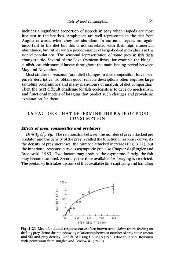
Density of prey. The relationship between the number of prey attacked per predator and the density of the prey is called the functional response curve. As the density of prey increases. the number attacked increases (Fig. 3.21). but the functional response curve is asymptotic (see also Chapter 8) (Ringler and Brodowski. 1983). Two factors may produce the asymptote. Firstly. the fish may become satiated. Secondly. the time available for foraging is restricted. The predatory fish takes up some of that available time capturing and handling

>­w C< 0..

o Z

200

2 40 4~0 720 960

PREY DENSITY/30 MIN

Fig. 3.21 Mean functional response curve often brown trout, Salmo trutta, feeding on drifting prey (brine shrimp) showing relationship between number of prey eaten (mean and SE) and prey density. Line fitted using Holling's (1959) disc equation. Redrawn with permission from Ringler and Brodowski (1983).

60 Feeding

each prey. At a sufficiently high prey density all the time available for foraging will be taken up (Holling. 1959).

Although the number attacked increases with density. prey at high densities are not always preferentially attacked. A threespine stickleback confronted with a swarm of Daphnia attacks the densest part of the swarm when it is hungry. As it becomes satiated. it switches to attacking less-dense regions of the swarm. although its rate of reward is lower (Milinski, 1977a. b; Heller and Milinski, 1979). A plausible explanation for the observation is that a high prey density imposes a high confusion cost. The attacker has more difficulty in focusing on anyone prey because there are numerous similar prey moving irregularly in its field of view and so has to attend closely to the task (Ohguchi. 1981). But this is at the cost of paying less attention to other events in the environment such as the approach of a predator (Heller and Milinski, 1979).

Effect of conspecifics. Many species forage in shoals. Experimental studies suggest that when food is distributed in patches a fish can increase its rate of feeding by joining a shoal (Pitcher. 1986). The median time taken by individual minnows. Phoxinus phoxinus. and goldfish. Carassius auratus. to find a randomly positioned food item decreases with shoal size (Fig. 3.22) (Pitcher et a!.. 1982). Fish foraging in a shoal recognize when another member of the shoal finds food. Threespine sticklebacks that see a conspecific assuming the head-down posture characteristic of a fish taking food off the bottom rush into the same area (Wootton. 1976). An individual minnow in a shoal devotes

160

r 120

80

40 t Vl • Cl 0 z

4 Cl u .., Vl

120 (bl

80

1 40 f ~ , 0

4 6 ~+o SHOAL SIZE

Fig. 3.22 Relationship between shoal size and median time spent before a randomly located food item was found by an individual fish (interquartile shown by vertical line); (a) goldfish. Carassius auratus; (b) minnows. Phoxinus phoxinus. Lines show medians quartiles for 16 replicates. Redrawn with permission from Pitcher (1986).

Rate of food consumption 61

75-

25-

4 6 12 20 SHOAL SIZE

Fig. 3.23 Effect of shoal size in minnow. Phoxinus phoxinus on time spent foraging (black shading). in weeds (vertical hatching). swimming in mid-water (horizontal hatching) and swimming at bottom (open). Redrawn with permission from Pitcher (1986).

more time to foraging than to predator-avoidance behaviour such as hiding in weed-beds than if it is on its own (Fig. 3.23) (Magurran and Pitcher. 1983) (see also pages 143-5).

Effect of predators. The presence of piscivores can reduce the food consumption of a fish because the fish is less likely to forage. In the presence of a potential predator juvenile coho salmon reduce the distance they will swim to catch a fly (Dill. 1983). A similar reduction in attack distance occurs in juvenile Atlantic salmon in the presence of a piscivore (Metcalfe et aI.. 1987).

The increased attentiveness required to overcome any confusion effect to exploit the high prey density detracts from the ability to be vigilant to other things such as the approach of a piscivorous fish or bird (Milinski. 1984a. 1986a). Food-deprived threespine sticklebacks exposed to a model of an avian piscivore switch from directing most attacks at the dense part of a swarm of Daphnia to attacking a less dense region (Milinski and Heller. 1978).

Hunger and appetite

If food is abundant and there are no other confounding factors such as the presence of predators. the rate of food consumption will be determined by the feeding motivation of the fish. Two systems control the rate of consumption: systemic demand. that is the demand for energy and nutrients generated by the metabolic rate (see Chapter 4). and secondly. the rate at which the digestive system can process food (Colgan. 1973). These two interact to generate the motivational state of hunger and to determine appetite. Hunger is the propensity to feed when given the opportunity. while appetite is the quantity of food consumed before the fish ceases to feed voluntarily.

The distinction between hunger and appetite is illustrated by experiments with the threespine stickleback. As the period for which sticklebacks are starved increases to 4 d. several components of their foraging behaviour

62 Feeding

change (Beukema. 1968). The distance swum. the number of bouts of search swimming. the proportion of discovered prey that are grasped and the proportion of grasped prey that are eaten all increase. Fish also direct more feeding attempts at inedible objects. These changes indicate increasing hunger. The amount of food eaten during the first 8 h after food is supplied in excess does not increase as the preceding period of starvation is increased from o to 4 d. However. the proportion ofthe total that is eaten in the first hour does increase. In brown trout. appetite measured as the amount of food consumed in 15 minutes remains close to zero as the number of hours since the last meal increases until a threshold period of deprivation is reached (Elliott. 197 Sa). Beyond that threshold. the amount eaten increases rapidly to an asymptote (Fig. 3.24).

Rate of gastric evacuation. The amount of food required to satiate a fish is related to the state of distension of the stomach (or foregut in fish that lack stomachs). The rate offood consumption is dependent on the rate at which the stomach contents are evacuated. Studies on the brown trout (Elliott. 1972) and fingerling sockeye salmon. Oncorhynchus nerka (Brett and Higgs. 1970) suggest that the rate of evacuation is described by a simple exponential model:

dS/dt = -kS

where dS/dt is the instantaneous rate of evacuation. S is the weight of stomach contents and k is the rate constant. This model states that the rate of evacuation is proportional to the weight of remaining contents. which means that the absolute rate of evacuation is highest immediately after the meal (Fig. 3.25). An exponential model describes gastric evacuation in many other

200

150 • • • •

c °E • o

o

'" e;, 100 o 5 0 0 0 "-

50

0 • 0

0 5 10 15 20 DEPR IV ATIO TIME (h)

Fig. 3.24 Effect of deprivation time and temperature on appetite (food consumed per 15 min) of brown trout at two temperatures. O. 6.8°C; •. 15.1 DC. Redrawn with permission from Elliott (1975b).

Rate of food consumption 63

Vl >-Z UJ Vl >- >-Z z a UJ w >-:J:

Z a

w w < L >-a >-

3 Vl I!J

>-a -'

3

TIME TIME

60

C, .5 Vl >-E:5 >-z a w

:J: w < L a >-Vl

>-3

0·5 15·0 12·1 9-8 7-6 5-2

0·2 0 12 18 24 30 36 42

HOURS

Fig. 3.25 Exponential gastric evacuation in brown trout. (a) Arithmetic plot of decline in stomach contents: (b) semi-log plot of decline: (c) effect of temperature over range 5.2-15.0 °C on rate of evacuation. Redrawn with permission from Elliott (1972).

species. although in some there is a time-lag between the ingestion of the meal and the exponential phase of evacuation. For fish that take large meals, at long intervals, the rate of evacuation may be linear rather than exponential. Other models of evacuation may be appropriate in some circumstances (Jobling. 1986).

The rate of evacuation increases with temperature (Fig. 3.25). In brown trout, the time taken to evacuate 90% of a meal of amphipods (Gammarus) decreases from 24 h at 5.2 °C to 8 h at 15.0 °C (Elliott, 1972). The quality ofthe food also influences the rate of evacuation: food with a low energy content is evacuated faster than food with a high energy content (Jobling, 1980). However, if a meal consists of a mixture of different prey, the rate of evacuation of each type of prey is not independent of the other items (Persson, 1984).

In brown trout and sockeye salmon appetite increases rapidly when about

64 Feeding

75-90% of the previous meal has been evacuated (Brett. 1971a; Elliott. 197 sb). These species eat medium-sized discrete food items such as inverte­brates or small fish. In contrast some filter-feeding fishes such as the menhaden may never become satiated. but ingest food continuously. Similarly de­tritivores such as the striped mullet. Mugil cephalus. which are exploiting a resource with a low energy content. may feed almost continuously. relying on a rapid turnover of the gut contents (Pandian and Vivekanandan. 1985).

Effect of temperature and other abiotic factors. Temperature affects the maximum rate of consumption through its effects on the rate of gastric evacuation (Fig. 3.25) and its effects on systemic demand. At low tempera­tures fish may cease to feed. but as the temperature increases. the rate of consumption also increases up to a maximum. Any further increase in temperature is marked by a rapid decrease in consumption (Fig. 3.26) (Elliott. 197 Sa. b. 1981). The optimum temperature for feeding is the temperature at which the highest rate of consumption occurs. In brown trout the increase in consumption with temperature reflects an increase both in the amount eaten in one meal and in the number of meals eaten in a day (Elliott. 197 Sa. b). The decline in consumption at high temperatures is a systemic effect because the rate of gastric evacuation continues to increase (Elliott. 1972).

In natural populations changes in the rate of consumption can be correlated with water temperature. though the causal effects of temperature may be confounded with those of other abiotic factors and changes in the availability of food. In Lake Opinicon. bluegills do not eat in winter but commence feeding in spring when the temperature reaches 8-10 °e. Feeding ceases in late autumn. The rate of consumption by the winter flounder in a New England salt pond also increases with temperature. ranging from a mean of 1.27% of dry body weight in April (6.5 0c) to 3.31% in September (22 °C) (Worobec. 1984).

2000

1000

0. 500 .§

8 a LL 100 LL a 50 l-I I!)

W 3

10g 10 >-0: 5g D

19

10 15 20 TEMPERATURE (Oe)

3.26 Effect of temperature on dry weight of food eaten in a meal by brown trout of different live weights. Redrawn with permission from Elliott (197 Sa).

Rate of food consumption 65

Abiotic factors other than temperature also influence the rate of consump­tion. In the threespine stickleback there is a significant reduction in consumption as the pH of the water declines from 5.5 to 4.5 (Faris. 1986). Light may have a direct effect: as the ambient light levels fall. the fish is unable to perceive food and feeding ceases (see page 47). Photoperiod may also influence the endocrine system and so indirectly cause changes in hunger or appetite (Peter. 1979; Matty and Lone. 1985).

Effect of body weight. The relationship between the maximum weight of food consumed over a period oftime. typically 24 h. and the weight of the fish is described by:

or in the linear form:

log C = log a + b log W

where C is weight of food consumed. W is weight of fish and a and bare parameters that can be estimated by regression analysis. For the brown trout. Elliott (1975a. b) shows that this relationship describes both the weight of food consumed during a meal and the total weight consumed in a day. The value of the exponent. b. is usually less than one (Table 3.4). As fish grow. the weight of food they consume relative to their body weight decreases. although the absolute weight consumed increases.

Effect of physiological state. Major changes in consumption can occur as the physiological state changes. In some species. the rate of feeding decreases or ceases as the fish become reproductively active. Well-known examples are

Table 3.4 Values for weight exponent (b) in relationship between food consumption (C) and body weight (W): C= aWb*

Temp. Species (DC) Food b

Ctenopharyngodon idella 23 Lettuce 0.80 Tubifex + lettuce 0.49

Esox spp. 5-30 Minnows 0.82 Gasterosteus aculeatus 3-19 Enchytraeus spp. 0.93 Phoxinus phoxinus 7-19 Tubifex spp. 0.56

5-15 Enchytraeus spp. 0.81 Salmo gairdneri 8-16 Fish 0.84

12 Pelleted food 1.1 5-26 Formulated diet 0.70-0.77

Salmo trutta 4-22 Gammarus 0.73-0.77 Solea solea 10-26 Mussel meat 0.40-0.94

*Source: Cui (1987).

66 Feeding

the anadromous salmonids which cease to feed during their upstream spawning migration, although they continue to strike at prey making them vulnerable to capture by anglers. (This suggests the paradox that the salmon are hungry but have no appetite!) During the upstream migration the gut undergoes degenerative changes which prevent any normal food processing (Brett, 1983).

Some marine fishes also cease to feed during their spawning migration or on the spawning grounds, for example the herring, Clupea harengus (Iles, 1974, 1984). Iles' analysis of the feeding and reproductive cycle of the North Sea herring is important because it illustrates the potential that fish have to control their rate of food consumption. The period of intensive feeding begins when temperatures are still low, but ceases when temperatures are relatively high and while food is still plentiful. Iles (1984) argues that the lack of a close relationship between the feeding activity ofthe herring and either temperature or food availability indicates that to a surprising extent the herring is independent of its thermal environment.

However, the effects that temperature and body weight do have on voluntary food consumption mean that if fish are being fed artificially, as in a hatchery or fish farm, the ration provided has to be adjusted as the fish grow and as the water temperature changes.

Methods of estimating food consumption in natural populations

Estimates of the rate of consumption by fish in natural populations are essential for three reasons: to assess the demands that fish make on their food resources, to assess the extent to which survival, growth and reproduction are limited by food availability and to estimate the energy and nutrients available for allocation between maintenance, growth and reproduction. Consumption can rarely be estimated by direct observation, so indirect methods must be adopted. These methods fall into two groups, those that rely on estimating the rate of passage of food through the gut and so give an instantaneous estimate of consumption, and those methods that integrate the consumption over a relatively long period and measure it by estimating the rate that would give the growth observed over that period (Wootton, 1986). They have the disadvan­tage that they usually give estimates of the mean rate of consumption for a population rather than for individuals.

A popular method for estimating food consumption assumes that if the consumption rate over a fixed period of time is constant, the rate at which the weight of the stomach contents changes can be written as:

dSjdt = C -kS

where S = weight of contents, dSjdt = rate of change of stomach contents, C = rate offood consumption and k is a rate constant assuming an exponential pattern of gastric evacuation (Elliott and Persson, 1978; Eggers, 1979). By

Rate of food consumption 67

integration. the following expression is derived:

Ct = ((St - Soe-kt)kt)/(l - e- kt)

where Ct is the weight consumed in the time interval 0 to t. So and St are the weights of stomach contents at times 0 and t respectively. and k is the evacuation rate (Elliott and Persson. 1978). Worobec (1984) gives formulae for putting confidence intervals on the estimate of Ct. This method can be used to estimate the daily consumption by taking samples of fish at intervals of 2-3 h throughout a 24 h period. The daily consumption. FD. is given as:

FD=~Ct

When the weight of stomach contents at the end of the 24 h period is the same as at the start. a simple estimate of FD can be obtained as:

FD= 24Smk

where Sm is the mean weight of stomach contents and k is the rate of evacuation with units h- 1 (Eggers. 1979). Field observations (Allen and Wootton. 1984) and a comparative study (Boisclair and Leggett. 1988) suggest that this simpler method can give estimates of daily consumption similar to those obtained with the Elliott and Persson method. The simpler method has the advantage of requiring a much reduced sampling effort.

To obtain the stomach contents from a sample. fish must be killed or stomach-pumped. A method of estimating food consumption which avoids these traumatic procedures depends on the quantitative collection ofthe faeces produced by the fish over a known time period (Allen and Wootton. 1983). Laboratory experiments provide information on the relationship between the weight offaeces produced and the weight offood consumed. which is then used to predict consumption from faecal production. For this method. the food used in the laboratory study must resemble the food the fish are consuming naturally.

A problem with methods which estimate the rate of consumption over a period of about a day is that there may be considerable day-to-day variation in the rate. Groups of largemouth bass kept at a constant temperature with food constantly present show highly significant changes in their daily consumption rates (Smagula and Adelman. 1982). Estimating food consumption for a relatively long period from the growth rate over that period avoids problems caused by day-to-day variations in consumption.

Methods that estimate consumption from growth fall into two categories. In the first. empirical relationships between growth and food consumption determined in laboratory studies are used to predict food consumption from growth rates observed in a natural population. In the second are those methods which assume that a balanced budget for some quantity. usually energy or nitrogen. can be calculated for individual fish. The input from the food must equal losses through defecation. excretion and metabolism plus the

68 Feeding

gain in the form of an increase in the energy (or nitrogen) content of the fish (see Chapter 4). This gain is measured as growth (see Chapter 6).

A simple formulation of an energy budget was developed by Winberg (1956) who suggested that food consumption could be estimated as:

0.8C=P+R

where C is food consumed over the time interval, P is the growth and R is total metabolism over the interval. all measured in energy units (see Chapter 4). Frequently R is estimated as twice the metabolic rate of a resting fish measured under laboratory conditions (see Chapter 4). Modifications and refinements of Winberg's original equation have been developed (Majkowski and Waiwood, 1981), but the original formulation is still used. Bioenergetics models developed to predict growth which are described in Chapter 6 can also be adapted to predict rates of consumption when growth rates are known.

Gerking (1962, 1972) estimates food consumption in a population of bluegill sunfish from a nitrogen budget by combining experimental studies on the relationship between nitrogen retention (growth) and consumption with observations on the growth rate in the natural population.

Each method makes assumptions which may not be valid for the population under study. Most methods also require that information obtained under laboratory conditions be extrapolated to a natural population. How reliable are estimates provided by these methods? Studies comparing estimates of natural rates of food consumption obtained by more than one method give an ambiguous answer.

Estimates of food consumption by perch in Windermere comparing results from Winberg's energy budget equation with estimates using the formula FD= 24Smk are in reasonable agreement (Craig, 1978). Both methods describe a similar pattern of seasonal change in consumption. In contrast, Minton and McLean (1982) compare estimates of consumption based on the Winberg method and from an analysis of stomach contents for a population of the piscivorous sauger, Stizostedion canadense, in a reservoir in Tennessee. For the period March to October, the estimates agree well, but over the winter months, the rate of consumption estimated from the stomach contents is much higher than that estimated from growth. A study of pike in Lac Ste Anne, Manitoba also finds poor agreement between estimates based on stomach contents and on a detailed energy budget: only four of 18 estimates are within 20% of each other (Diana, 1983a). A comprehensive study estimated the rate of food consumption by a population of threespine sticklebacks in a small Welsh lake by using the methods of Elliott and Persson (1978), the rate of faecal production, growth rate and by calculating a balanced energy budget (Allen and Wootton, 1984; Wootton, 1984a; Wootton, 1986). With one exception the methods give estimates for the annual consumption per fish of between 2.3 and 4.2 g wet weight. Although this similarity suggests that independent methods can give comparable results, it is partly coincidental

Flexibility in feeding ecology 69

20

16

I-12

::r::

"" ;;:; 3

>-8

0 a a:l

~

MONTH

Fig. 3.27 Estimates of seasonal changes in daily rate of food consumption (% body fresh weight) by an average-size threespine stickleback. Gasterosteus aculeatus. in Llyn Frongoch. Mid-Wales. Estimates from: D. rate of faecal production; •. growth rate; •. Elliott and Persson's (1978) method; O. weight of stomach contents (two meals per day). Redrawn with permission from Wootton (1986).

because the methods give different pictures of seasonal changes (Fig. 3.27) (Wootton. 1986). Nevertheless. the study suggests that as methods are refined. reasonably accurate estimates of consumption can be achieved. although the use of more than one method is probably advisable.

Before consideration of the uses to which the energy in the food is put. an important feature of the feeding ecology of many fishes must be emphasized.

3.7 FLEXIBILITY IN THE FEEDING ECOLOGY OF FISHES

Any attempts at generalizations on the feeding ecology of fishes confront the problems posed by the trophic flexibility that many species show. Examples of this flexibility are provided by comparisons between individuals. as well as by the ontogenetic. seasonal and diel changes in diet that have already been described. Fish from the same population sampled at approximately the same time and place can have significantly different diets (Bryan and Larkin. 1972; Ringler. 1983). Some of these differences may reflect individual variation in physiological and morphological characteristics (Ringler. 1983). Even for the bluegill sunfish. a species commonly described as a generalist feeder. there is some evidence of specialization by individual fish. In a pond experiment. the bluegills initially foraged in vegetation but when this habitat became depleted of prey they switched to more profitable habitats. Some individuals specialized as foragers in open water and others as foragers on benthic invertebrates living

70 Feeding

in sediments (Werner et al.. 1981). A careful comparison of the feeding behaviour and morphology of blue gills from a small lake in Michigan identifies individual fish that tend to be specialized for foraging in either a littoral or an open-water habitat (Ehlinger and Wilson. 1988). A generalist population is made up of partial specialists (see also Chapter 9). Another source of variation is the behavioural flexibility of individual fish which move to habitats of greater profitability or change their preferences (Werner et aI.. 1981). Individual brown trout that are fed meal-worm larvae and tent caterpillars in different proportions show changes in preference both within a 30 min period and over a period of days (Ringler. 1985). Sometimes individual preferences result in fish with bizarre diets. A brown trout caught in an upland Welsh lake had about 150000 ostracods in its gut (Whatley. 1983). although these microcrustaceans normally form only a minor component of the diet oftrout in that lake (AI-Shamma. 1986).

Fish may switch from one type of prey to another as the relative abundance ofthe prey types changes (Murdoch and Oaten. 1975). Changes in diet are well known in generalist feeders such as sunfish. perch and trout (Keast. 1978). but they also occur in species that seem to be specialized for exploiting particular foods. In Lake Victoria. cichlids. which are typically zooplanktivores. in­sectivores or detritivores switch to feeding on a diatom. Melosira. when it becomes superabundant (Witte. 1984).

Ontogenetic and seasonal changes in diet frequently involve a change in its taxonomic composition. A rock bass shifts from feeding on zooplankton as a larva and juvenile. to feeding on the larvae and nymphs of invertebrates and finally ends up as a piscivore. Some species that are herbivorous as adults include animal food in their diet when they are young. The proportion of plant and animal food in the diet can change seasonally. Cichlasoma panamense is a stream-living Central American cichlid. In a population living in a small Panamanian stream. the proportion of algae in the diet is greatly increased during the dry season (Townshend. 1984). Such changes make it difficult to categorize many species of fish in terms of the well-established ecological concept of trophic levels. i.e. herbivore. primary carnivore. secondary carnivore or detritivore (cf. Table 3.1). An alternative method of analysing the trophic relationships of many assemblages of fishes may be a description of the rate of exploitation of food items of different sizes by fishes of different sizes (Parsons and Le Brasseur. 1970; Werner and Gilliam. 1984).

Within a species. differences in the diet composition at different stages in the life history or between populations can be reflected in morphological differences (Kapoor et aI.. 1975; Weatherley and Gill. 1987). The striped mullet feeds on micro algae and decaying plant detritus and its gut often contains quantities of inorganic sediment. A comparison of two populations shows that the increase in gut length as fish length increases is significantly greater in the population whose diet includes a high proportion of plant detritus than in the population whose diet includes a high proportion of

Summary and conclusions 71

benthic and epibenthic diatoms (Odum, 1970). Sibly (1981) used a cost­benefit model to predict that within a population, relative gut length would change with a change in the quality of the diet. A possible example of this is shown by CichIasoma panamense. The change to herbivory in the dry season is associated with an increase in relative gut length in the population (Townsh­end, 1984).

Some morphological differences between populations reflect an evolution­ary process. The Cowichan drainage system in British Columbia (Canada) includes several lakes which range in surface area from 1.4 to 6180 ha. Threespine sticklebacks from these lakes show significant interpopulation variation in morphological features related to their trophic ecology, including the length ofthe upper jaw and the number and length of the gill rakers (Lavin and McPhail, 1985). Sticklebacks from the smallest lakes have a morphology and behavioural repertoire that enables them to feed on benthic prey more effectively than fish from the larger lakes, whereas the latter are more effective at feeding in the water column (Lavin and McPhail, 1986). These interpopul­ation differences have probably evolved since the last Pleistocene glaciation, that is in the last 10 000 y. This gives an estimate of the rate of evolution of ecologically significant morphological and behavioural characteristics.

A spectacular example of evolutionary plasticity in relation to feeding is the extraordinary adaptive radiation of the cichlids in the African Great Lakes (Fig. 3.7). This single family within restricted geographical and physical localities has evolved to exploit virtually every type of resource that is exploited by the teleosts as a group (Fryer and lies, 1972). The processes that have led to this evolutionary flowering are still under active discussion (Echelle and Kornfield, 1984), but the African Great Lakes cichlids provide a unique test­bed for ecological and evolutionary theories on the biology of feeding. Sadly, the cichlid fauna of Lake Victoria is threatened by the piscivorous Nile perch, Lates niloticus, introduced into the lake in about 1960 (Barel et aI., 1985), (see page 329).

3.8 SUMMARY AND CONCLUSIONS

1. Fishes show a wide adaptive radiation in their feeding habits. They occupy many trophic roles from detritivores to carnivores. There is often a correlation between morphological traits and trophic role because morphology determines how a fish can feed. Body shape, mouth morphology, teeth, gill rakers and the structure of the alimentary canal can all be related, in a general way, to diet.

2. Several methods are available for describing diet composition on the basis of either the number or the bulk of food items present in a diet. No single method is entirely satisfactory, and the best methods for the statistical analysis data on diets are still under debate.

72 Feeding

3. The presence of a food item in a diet depends on its availability. its detection by the fish and its selection as food. For many carnivorous fishes. including zooplanktivores. vision is the most important sensory modality for prey detection. Prey selection also depends on the mechanical ability of the fish to manipulate the prey successfully. Selection may also depend on the profitability of the prey. Optimal foraging theory has been used with some success to predict the diet composition of some species on the basis of prey profitability.

4. Factors involved in the selection of food by herbivores or detritivores are less well understood.

5. Diet composition often changes as a fish grows (ontogenetic diet changes). so a fish may adopt several trophic roles in its lifetime. Diel and seasonal changes in diet may also occur.

6. The rate of food consumption is determined by the availability of food and the motivational state of the fish. The rate is affected by temperature and other abiotic factors. by body size and by the physiological condition of the fish.

7. Estimates of the rate of consumption by fish in natural populations can be obtained from calculations based on the rate at which the gut is evacuated or from estimates of the amount of food required to provide the energy and nutrient requirements of the fish.

8. Many fishes are flexible in their choice offoods. responding to changes in the availability or profitability of potential prey. Even species with specialized morphological adaptations related to feeding may show surprising flexibility in their choice of food.

9. There is evidence that morphological and behavioural traits related to feeding may show rapid evolutionary change. This reflects the central importance of feeding as the activity which provides the resources required for maintenance. growth and reproduction.

10. The goal of studies of the ecology of feeding must be to develop models which predict the composition and quantity of the food consumed. The quality and amount consumed determine the energy available to a fish. The patterns of allocation of this energy form the subject of the next four chapters.