Ecole d’Eté 2014 - obs-mip.fr · Traitement de la mesure : des formes d’onde • Elément essentiel du système altimétrique : mais un des ... direct, precise measurements of

Ecole d’Eté 2014

Ecole d’Eté 2014

Altimétrie spatiale

Traitement de la mesure : des formes d’onde

au bilan de performance système

N. Picot / CNES Toulouse

Ecole d’Eté 2014, Saint-Pierre d’Oléron, 1-5 septembre 2014 1

Ecole d’Eté 2014 2

Traitement de la mesure : des formes d’onde au bilan de performance

système

• ….De la forme d’onde …


OGDR

3 hours

IGDR

1 to 1.5 days

GDR

40 days

GOALS

Altimeter noise 1.7 (a)(c)(d) 1.7 (b)(c)(d) 1.7 (b)(c)(d) 1.5 (b)(c)(d)

Ionosphere 1 (e)(d) 0.5 (e)(d) 0.5 (e)(d) 0.5 (e)(d)

Sea State Bias 3.5 2 2 1

Dry troposphere 1 0.7 0.7 0.7

Wet Troposphere 1.2 1.2 1.2 1

Altimeter range

RSS

4.5 3 3 2.25

RMS Orbit

(Radial component)

6.8 (h) 2.5 1.5 1

Total RSS sea surface

height

11.2 3.9 3.4 2.5

Significant wave

height

10% or 0.5 m (i) 10% or 0.4 m (i) 10% or 0.4 m (i) 5% or 0.25 m (i)

Wind speed 1.6 m/s 1.5 m/s 1.5 m/s 1.5 m/s

Sigma naught

(absolute)

0.7 dB 0.7 dB 0.7 dB 0.5 dB

System drift 1mm/year (j)

Table 6 : JASON-3 ERROR BUDGET (in centimeters)(for 1 sec average, 2 meters SWH, 11 dB sigma naught)

• A la performance système :


Traitement de la mesure : des formes d’onde

• Elément essentiel du système altimétrique : mais un des

contributeurs parmi d’autres

• Très variable selon les différentes surfaces survolées :

– L’altimètre fonctionne en continu et fournit une intégrale de l’énergie très

dépendante de la nature du terrain – topographie mais aussi rugosité.

– Information discrète avec une résolution spatiale (distance) relativement faible

(environ 45 cms) par rapport aux attentes des utilisateurs (1.5 cms)

– Des évolutions technologiques récentes : le mode SAR (Altimètrie Doppler Along

track)

– Ne couvre pas la future mission SWOT (interférométrie)

• au bilan de performance système :

– Fortement dépendant des applications concernées,

– Actuellement principalement sur les surfaces ‘océaniques’ : traduit la précision de

détermination de la hauteur de mer et la stabilité temporelle requise pour les

applications de type ‘Niveau de la mer’.

– Dépendant de nombreuses méthodes élaborées de traitement, de moyens de

validation et de comparaison

– Et bien sur d’équipes en charge des ‘opérations-traitements-validations-évolutions-

User_services- …. ‘, de scientifiques associés au projet, …

Ecole d’Eté 2014

• Quelques mots sur la circulation :

La topographie signature des

courants géostrophiques

• Quelques mots sur les

exigences/attentes des utilisateurs

• Le système altimétrique et les

techniques de traitement

• L’observation obtenue avec une

mission : le besoin de

combinaison.

Ecole d’Eté 2014

The Ocean is moving all around

An exemple: The Gulf Stream travels at ~ 4 km/hourtransports ~ 80 millions tonnes/second

Why decoding the Ocean?

Ecole d’Eté 2014

7

Sea surface topography reveals ocean circulation Ocean Topography as seen from space by TOPEX-POSEIDON (or any other altimetric mission)

Sea surface topography reveals ocean circulation Ocean Topography as seen from space by TOPEX-POSEIDON (or any other altimetric mission)

Sea surface topography reveals ocean circulation : the geostrophic equilibrium

Ecole d’Eté 2014

8

A simple model: the geostrophic equilibrium

•Main long wavelength ocean currents are geostrophic currents:

•Coriolis force balanced by gradient of the horizontal pressure force due to the slope of the sea surface (geostrophic equilibrium)

•always perpendicular to the pressure gradient•Currents are deduced from the maps of Sea Level Anomaly

•Generation of geostrophic currents on an oceanic bump in the northern hemisphere

Coriolis force

Geostrophic current

Horizontal pressure force

Sea surface topography reveals ocean circulation


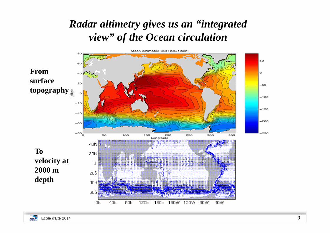
Radar altimetry gives us an “integrated view” of the Ocean circulation

From surface topography

To velocity at 2000 m depth

Sea surface topography reveals ocean circulation


A very large set of applications

Coastal

Altimetry and oceanography

Ecole d’Eté 2014

Variations du niveau moyen des océans

Dynamique océanique:Courants, tourbillons, marées, ‘el niño’

Géoïde et circulation grande échelle

Météo marine: vent, vagues

11

Sur océan : Que voit-on avec les données altimétriques ?

Ecole d’Eté 2014

10 km

Ocean oscillation (El

Niño, Pacific Decadal

Oscillation, North

Atlantic Oscillation).Major currents

(Gulf Stream,

etc).Eddies, tides.

Waves, cyclones,

storms.

100 km

1,000 km

10,000 km

To study wide spatial and temporal scales

Spatial scales

Ecole d’Eté 2014

Time scales

1 century

10 years

100 days

10 days

1 day

Variations in global

mean sea level.

North Atlantic and Pacific

oscillation;

recurrence of phenomena

such as El Niño.

Seasonal

variations.

Variations in typical

eddies.Variations due to tides,

winds, eddies in areas of

major activity, storms

and cyclones.

Ecole d’Eté 2014

14

Varying amplitude

The amplitude of

the observed

phenomena

ranges from a

few tens of

metres to several

millimetres for

the mean sea

surface height

signal.

4 000

2 000

0

-2 000

-4 000

2 000

1 000

0

- 500-1 000

500

1 500

400

200

0

- 200

Latitude Latitude Latitude

Geoid undulations:

Amplitude of a

several tens of

metres.

Major western

boundary currents:

Amplitude of about 1

metre.

Mesoscale

circulation:

Amplitude of about 1

decimetre.

Ecole d’Eté 2014

15

- Higly performing radar altimeters- Precise orbit determination systems- Additional systems (e.g. radiometer)

Key components of an altimetric mission

Altimetry system and altimeter data processing

Ecole d’Eté 2014

16

Precision of the SSH:

•Orbit error

•Errors on the range

• Instrumental noise

•Various instrument errors

•Various geophysical errors (e.g., atmospheric attenuation, tides, inverse barometer effects, …)

Sea Surface Height (SSH) (relative to an earth ellipsoid)= Orbit height – Range

SSH = Orbit – Range – ΣCorr

Orbit errors in position of satellite

Principles of radar altimetry. SSH measurements

Ecole d’Eté 2014

Sampling of the waveform

xxxxxxxxxxxxxxxxxx x x x x x x x x x x x x x x x x x x

64 samples (ERS, Poseidon-1)

128 samples (Topex, Poseidon-2 and 3, RA2)

Power

Frequency/time/distance

10 KHz ≡≡≡≡ 3.125 ns ≡≡≡≡ 47 cm

The range resolution of an altimeter is about half a metre (3.125 ns) but the

range measurement performance over ocean is about one order of

magnitude better. This is achieved by fitting the shape of the echo waveform

to a model function which represents the form of the echo (Brown, Hayne) +

averaging over a large number of echoes (PRF > 2000 Hz)

Ecole d’Eté 2014

Nadir altimeter • Altimeter over ocean: Classical Brown model

• Basic assumption:homogeneity of the surface backscatter over the footprint

• Not true in presence of small island, surface slick, currents etc.. i.e. Strong variations of surface backscatter at scale < footprint size

• In such cases: altimeter can be seen as an imager of the surface backscatter whose geometry is annular and not rectangular

Ecole d’Eté 2014

Radar Equation

Radar equation

(in the case of a

punctual target)

σπλ

= 243

20

e2

r GR)4(

PTP

σ : backscattering section

Extended target = Sum of all the elementary scattering cells on the S surface

∫σ=σSurface

0dS σ0 : backscattering coefficient

(sigma naught)

Example : POSEIDON2 emits 5W with SNR=20 dB if σ0=11dB

Ecole d’Eté 2014

Mathematical formulation of the echo

)t(PFs)t(Q)t(RI)t(S ⊗⊗=RI(t) : Point target response of the radar

Q(t) : Probability density function of the scatterers

PFs(t) : Radar response to a calm sea to a short pulse

+γ

=α

eRh

1h

c4

2s

2p

2c σ+σ=σ )

2(sin.

)2(Log.21 02

e

θ=γ

Formulation of the HAYNE’s model (simplified form without skewness)

n

2c

c

2cu P

2texp

2

terf1

2

P)t(S +

ασ−τ−α−

σασ−τ−

+=

with T5.0p =σ

)c2/(SWHs =σ

Application à SARAL : vous avez 2 heures ….

Ecole d’Eté 2014

Retracking function : on-ground processing

For each averaged waveform (20Hz), fitting procedure between a model and the measured waveform

Energy of the pulse :

backscatterPu :

Slope of the trailing edge :

antenna mispointing

x :

Leading edge slope

Wave height

SWH :

Time to reach mid-power point

Distance, Rt :

Instrument noise Pb :

t

Ecole d’Eté 2014

50 100

After 1 iteration50 100

After 2 iterations

0 50 100

After 3 iterations50 100

After 5 iterations

0 50 100

After 7 iterations

50 100

After 10 iterations

Retracking algorithm :

Iterative fitting procedure (LSE) solving for N parameters (range, SWH, Pu, ξξξξ2, λλλλs, TN, ...)

Many possible solutions

� On each waveform

� On packet of waveforms


Satellite orbits are the reference frame for the altimetric measurements. T/P flies at 1336 km altitude and the satellite’s exact position needs to be accurately determined.

• An error in the radial orbit component (z) produces the same magnitude error in SSH.

• An error in the satellite’s alongtrack position, multiplied by the orbit slope, gives an error in SSH.

• An error in the onboard clock is similar to an error in alongtrack position

Precise orbit determination is made by specialist teams at the space agencies, using:

• force perturbation models on the satellite

• tracking data.

Satellite Altimetry Orbits


Satellite tracking is also made usingcomplementary systems : Laser tracking, DORIS and GPS

Satellite Laser Ranging (SLR).

A network of laser ground stations makedirect, precise measurements of the distance between the satellite and the laser ground station.

GPS

An onboard GPS receiver provides precise, continuous tracking of thesatellite by monitoring range and timing signals from up to 12 GPS satellites at the same time.

Satellite Tracking Systems … Laser Tracking and GPS



Altimeter measurements of sea surface topography are affected by a large number of errors :

• propagation effects in the troposphere and the ionosphere, electromagnetic bias,

• errors due to inaccurate ocean and terrestrial tide models, residual geoid errors,

• inverse barometer effect.

Some of these errors can be corrected with dedicated instrumentation : dual-frequency altimeter for ionospheric correction and radiometer for wet tropospheric correction.

Errors on altimeter measurements


Ecole d’Eté 2014

• Oscillator Drift Error : - Altimeter measures time by counting oscillator cycles- Error is due to a drift in the oscillator frequency (of the order of 1 cm)

• Doppler Shift Effect : - due to the relative velocity between the satellite and the sea surface- depends on the range rate, and the emitted frequency - range errors of + - 13 cm for the Ku band, +-5 cm for C band

• Internal Calibration- internal transit time in the altimeter- correction is a few cm

• Pointing angle error- Off-nadir pointing errors impacts the return pulse shape- Processing algorithms allow to compensate for this effect (up to 0.7°pointing error), but side effects are encountered on estimatedparameters (trailing edge)

Instrumental Corrections …



Dry TroposphereThe mass of dry air molecules in the atmosphere causes a range delay called the dry tropospheric effect. It is directly proportional to the surface pressure, with an average magnitude of 2.3 m (over the ocean). This correction is computed using atmospheric model pressure forecasts. The error is of the order of 1 cm / 4 mbar, or on average 0.7 cm.

Wet TroposphereThe range delay due to the atmospheric water vapor, the wet tropospheric effect, varies considerably both spatially and temporally, with magnitudes from 5 cm to 30 cm (maximum in the tropical convergence zones, where atmospheric convection is important).

The wet tropospheric correction is computed using either the on-board microwave radiometer measurements, with a precision better than 1.7 cm, or the water vapor content is calculated from atmospheric models.

Range Delay due to Atmospheric Refraction



Wet troposphere content as seen by Topex radiometer



•The radar pulse is delayed in the ionosphere (altit ude of 50 - 2000 km) due to the presence of electrons, produce d by the ionization in the high atmosphere by the incide nt solar radiation.

•The range delay is related to the EM radiation freq uency, so the correction can be estimated using two different radar frequencies (e.g. TOPEX, or DORIS). Otherwise estim ated from models of the vertically integrated electron d ensity.

•The delay can produce range errors from 1 to 20 cm. The accuracy of the dual-frequency correction is 0.5 cm .

Ionospheric Refraction



Spatial distribution•the Total electron

count is mainly

correlated to the

geomagnetic field,

maximum in the

tropical band

•the highest

electronic

perturbation

occurs at about

400 km altitude

Ionospheric Correction – spatial variability



•Temporal variability•Strongly diurnal,

maximum at 2 pm and

minimum around 5 am

•the TEC has seasonal

variations

•the TEC is correlated with

the solar activity (sunspots),

and the geomagnetism

Ionospheric Correction – temporal variability



Electromagnetic bias

The concave form of wave troughs tends to concentrate and better reflect the altimetric pulse. Wave crests tend to disperse the pulse. So the mean reflecting surface is shifted away from mean sea level toward the troughs.

Mean Sea Level

Mean Reflecting Surface

Sea State Effects



Skewness bias

For wind waves, wave troughs tend to have a larger surface area than the pointy crests – the difference leads to a skewness bias.

Again, the mean reflecting surface is shifted away from mean sea level toward the troughs

The EM Bias and skewness bias (= Sea State Bias or S SB) vary with increasing wind speed and wave height, but in a non -linear way.

SSB is estimated using empirical formulas derived from altimeter data analysis (crossover, repeat-track differences and parametric/non-parametric methods). The range correction varies from a few to 30 cm. SSB bias accuracy is ~2 cm.

Empirical estimation of the SSB also includes tracker bias (depends on H1/3).

Sea State Bias



Use of non-parametric methods to estimate SSB (SWH, Wind) (Labroue, 2007)

-30 cm 0 cm -30 cm 0 cm

Sea State Bias

Jason SSB Topex LES SSB



SSH = Orbit Altitude - Range – corrections

ΣΣΣΣ corrections =

• instrumental corrections

• sea state bias corrections

• ionospheric correction

• tropospheric corrections (wet, dry)

•Tides (ocean, earth) + Inverse barometer

Errors = errors in orbit, in corrections and instru mental noise

Corrected Altimetric Sea Surface Heights


Ecole d’Eté 2014

➪ Altimeter

● Instrumental noise 1.7 ● E-M bias 2.0● Skewness 1.2● Ionospheric corr. 0.5● Wet Tropospheric corr. 1.1 ● Dry tropospheric corr. 0.7● SWH 0.2 m● Wind Speed 2 m/s

➪ Range total error 3.2 cm

➪ Orbit error (radial) <1.5 cm (T/P-Jason-1) < 2.5 cm (ENVISAT)

➪ Instantaneous sea level error <3.5 cm (T/P-Jason-1)<4.1 cm (ENVISAT)

Performances

Topex-Poseidon – Jason-1 – ENVISAT



Oceanic signal

0

10

20

30

40

50

60

70

80

90

orbit errorRA errorIonosphereTroposphereEM Bias

100Centimeters

Geos 3 SEASAT GEOSAT ERS T/P(before launch)

T/P(after launch)843 km

115°various repeat cycles

800 km108°3 days

800 km108°17 days (ERM)

780 km98.5°35 days(3/168)

1336 km66°

9.95 days

EMR

PRARE TMR

GPS/DORIS

Jason-1/2ENVISAT

Error Budget for altimetric missions


Ecole d’Eté 2014

• Spatial coverage :

TOPEX/Poseidon or Jasons Sampling

- global

- homogeneous

• Temporal coverage :- repeat period10 days, T/P-Jason-1/217 days, GFO35 days, ERS/ENVISAT

1 measure/1 s (every 7 km) all weather (radar)

- Nadir (not swath)

Exact repeat orbits (to within 1 km)

Satellite altimetry coverage



780 km98°

35 daysENVISAT

1336 km66.03°

9.915 days 1h52

Jason-1

Repeat Period and Groundtracks



Sampling Issues

• How many altimeters are needed to

monitor the ocean circulation ?

• Difficult issue. Depends on objectives (e.g.

large scale circulation).

• Mesoscale variability sampling is a major

objective for altimetry.

Sampling issue


To better understand the ocean circulation and its role on climate, one needs to resolve the mesoscale

variability

This is also required for most of the operational applications (e.g. marine safety, pollution monitoring, offshore industry, fisheries).

Two altimeter missions at leastare needed to get a “good” representation of mesoscale

variability (e.g. Koblinsky et al., 1992).

Complementarity of Jason-1 and ENVISAT

Mesoscale variability : a key factor

Sampling issue


Subsample model fields (sea level anomaly) along altimeter tracks. Add a random noise.

Use of a sub-optimal space/time mapping method to reconstruct the 2D sea level anomaly signal from simulated along-track data.

Compare the reconstructed fields with the reference (model) fields(sea level and velocity) => allows an estimation of the sea level and velocity mapping error

Add extra noise and compare the reconstructed fields with the 10-day average fields=> allows an estimation of the mapping errors on 10-day average fields

Simulations with the Los Alamos model(Le Traon et al., 2001 and Le Traon and Dibarboure, 2002)

Mapping capabilities of Jason-1 (T/P) + ENVISAT (ERS)

Sampling issue


LAM rms SLA

Rms Mapping

error

Sea level mapping error from Jason-1+ENVISATsimulated from the Los Alamos Model (instantaneous and 10-day averaged fields)

Sampling issue


Sea level can be mapped with an accuracy of 5 to 10% of the signal

variance

Velocity mapping error from 20 to 40% of the signal variance

A large part of the mapping errors is due to high frequency (< 20 days) and high wave numbers signals.

Errors on 10-day averages are much smaller.

Summary of Jason-1 + ENVISAT mapping capabilities

Sampling issue


[c] 1998 D.B. Chelton

ERS/EN repetitivity

ER

S/E

N in

ter-

trac

k

TP

/J1

inte

r-tr

ack

TP/J1 repetitivity

Alo

ng-t

rack

res

olut

ion

Global sea level variability

Sea surface circulation variability /

Mesoscale activity

�

� Merging information from different altimeters leads to a better representation of the surface state (but not complete …)

45

Not a ll the physical processes are observable with the altimeterNot all the physical processes are observable with the altimeter


�� Geostrophic speed anomalies (U’, V’) computed by finite differences

�� EKE = ½ * (U’² + V’²)

Mean EKE (cm2/s2)

J1E2TPG2J1E2TPJ1E2J1

MERGING SATELLITE DATA Eddy energy

Sampling issue


MERGING SATELLITE DATA Jason-2 and Jason-1 flying in tandem


Integrated

Operational

Oceanography

Space Observation

In situ Observation

Assimilation Model

Developing a permanent global observation system

Documents

Ecole d’Eté 2014 - obs-mip.fr · Traitement de la mesure : des formes d’onde • Elément essentiel du système altimétrique : mais un des ... direct, precise measurements of