ÉCOLE DE TECHNOLOGIE SUPÉRIEUREUNIVERSITÉ DU QUÉBEC

THESIS PRESENTED TOÉCOLE DE TECHNOLOGIE SUPÉRIEURE

IN PARTIAL FULFILLMENT OF THE REQUIREMENTS FORTHE DEGREE OF DOCTOR OF PHILOSOPHY

Ph.D.

BYMIRANDA DOS SANTOS, Eulanda

STATIC AND DYNAMIC OVERPRODUCTION AND SELECTION OF CLASSIFIERENSEMBLES WITH GENETIC ALGORITHMS

MONTREAL, FEBRUARY 27, 2008

c© Copyright 2008 reserved by Eulanda Miranda Dos Santos

THIS THESIS HAS BEEN EVALUATED

BY THE FOLLOWING BOARD OF EXAMINERS :

Mr. Robert Sabourin, thesis directorDépartement de génie de la production automatisée at École de technologie supérieure

Mr. Patrick Maupin, thesis co-director

Recherche et développement pour la défense Canada (Valcartier), groupe de monotoringet analyse de la situation

Mr. Pierre Dumouchel, committee presidentDépartement de génie logiciel et des technologies de l’information at École detechnologie supérieure

Mr. Jean Meunier, external examinerDépartement d’Informatique et Recherche Opérationnelle at Université de Montréal

Mr. Éric Granger, examinerDépartement de génie de la production automatisée at École de technologie supérieure

THIS THESIS WAS PRESENTED AND DEFENDED

BEFORE A BOARD OF EXAMINERS AND PUBLIC

ON FEBRUARY 22, 2008

AT ÉCOLE DE TECHNOLOGIE SUPÉRIEURE

ACKNOWLEDGMENTS

I would like to acknowledge the support and help of many people who encouraged me

throughout these years of Ph.D. It is not possible to enumerate all of them but I would like

to express my gratitude to some people in particular.

First, I would like to thank my supervisor, Dr. Robert Sabourin who has been source of

encouragement, guidance and patience. His support and supervision were fundamental for

the development of this work.

Thanks also to Patrick Maupin from Defence Research and Development Canada, DRDC-

Valcartier. His involvement along the course of this research helped make the thesis more

complete.

I would like to thank the members of my examining committee: Dr. Éric Granger, Dr.

Jean Meunier and Dr. Pierre Dumouchel, who has made valuablesuggestions to the final

version of this thesis.

Thanks to the members of LIVIA (Laboratoire d’imagerie, de vision et d’intelligence

artificielle) who contributed to a friendly and open research environment. Special thanks

to Albert Ko, Carlos Cadena, Clement Chion, Dominique Rivard, Eduardo Vellasques,

Éric Thibodeau, Guillaume Tremblay, Jonathan Milgram, Luana Batista, Luis Da Costa,

Marcelo Kapp, Mathias Adankon, Paulo Cavalin, Paulo Radtkeand Vincent Doré.

ii

This research has been funded by the CAPES (Coordenação de Aperfeiçoamento de Pes-

soal de Nível Superior), Brazilian Government, and DefenceResearch and Development

Canada under the contract W7701-2-4425. Special thanks to people from CAPES and

Defence Research and Development Canada, DRDC-Valcartier, who have had the vision

to support this project.

I am indebted to Marie-Adelaide Vaz who has been my family andbest friend in Montreal.

Words cannot express how grateful I am for everything you have done for me. I also would

like to thank Cinthia and Marcelo Kapp, who besides friends,have been very special trip

partners. I am also indebted to my family for their love, support, guidance and prayers,

not only throughout the years of my PhD, but, throughout my life. To them is all my love

and prayers.

Finally, all thanks and praise are due to God for giving me thestrength and knowledge to

complete this work, "for from him and through him and to him are all things. To him be

the glory forever!"

STATIC AND DYNAMIC OVERPRODUCTION AND SELECTION OFCLASSIFIER ENSEMBLES WITH GENETIC ALGORITHMS

MIRANDA DOS SANTOS, Eulanda

ABSTRACT

The overproduce-and-choose strategy is a static classifierensemble selection approach,which is divided into overproduction and selection phases.This thesis focuses on the se-lection phase, which is the challenge in overproduce-and-choose strategy. When this phaseis implemented as an optimization process, the search criterion and the search algorithmare the two major topics involved. In this thesis, we concentrate in optimization processesconducted using genetic algorithms guided by both single- and multi-objective functions.We first focus on finding the best search criterion. Various search criteria are investigated,such as diversity, the error rate and ensemble size. Error rate and diversity measures aredirectly compared in the single-objective optimization approach. Diversity measures arecombined with the error rate and with ensemble size, in pairsof objective functions, toguide the multi-optimization approach. Experimental results are presented and discussed.

Thereafter, we show that besides focusing on the characteristics of the decision profiles ofensemble members, the control of overfitting at the selection phase of overproduce-and-choose strategy must also be taken into account. We show how overfitting can be detectedat the selection phase and present three strategies to control overfitting. These strategiesare tailored for the classifier ensemble selection problem and compared. This comparisonallows us to show that a global validation strategy should beapplied to control overfittingin optimization processes involving a classifier ensemblesselection task. Furthermore, thisstudy has helped us establish that this global validation strategy can be used as a tool tomeasure the relationship between diversity and classification performance when diversitymeasures are employed as single-objective functions.

Finally, the main contribution of this thesis is a proposed dynamic overproduce-and-choose strategy. While the static overproduce-and-chooseselection strategy has tradi-tionally focused on finding the most accurate subset of classifiers during the selectionphase, and using it to predict the class of all the test samples, our dynamic overproduce-and-choose strategy allows the selection of the most confident subset of classifiers to labeleach test sample individually. Our method combines optimization and dynamic selectionin a two-level selection phase. The optimization level is intended to generate a populationof highly accurate classifier ensembles, while the dynamic selection level applies mea-sures of confidence in order to select the ensemble with the highest degree of confidencein the current decision. Three different confidence measures are presented and compared.Our method outperforms classical static and dynamic selection strategies.

SURPRODUCTION ET SELECTION STATIQUE ET DYNAMIQUE DESENSEMBLES DE CLASSIFICATEURS AVEC ALGORITHMES GÉNÉTIQUES

MIRANDA DOS SANTOS, Eulanda

RÉSUMÉ

La stratégie de "surproduction et choix" est une approche desélection statique des ensem-bles de classificateurs, et elle est divisée en deux étapes: une phase de surproduction etune phase de sélection. Cette thèse porte principalement sur l’étude de la phase de sélec-tion, qui constitue le défi le plus important dans la stratégie de surproduction et choix. Laphase de sélection est considérée ici comme un problème d’optimisation mono ou multi-critère. Conséquemment, le choix de la fonction objectif etde l’algorithme de recherchefont l’objet d’une attention particulière dans cette thèse. Les critères étudiés incluentles mesures de diversité, le taux d’erreur et la cardinalitéde l’ensemble. L’optimisationmonocritère permet la comparaison objective des mesures dediversité par rapport à la per-formance globale des ensembles. De plus, les mesures de diversité sont combinées avecle taux d’erreur ou la cardinalité de l’ensemble lors de l’optimisation multicritère. Desrésultats expérimentaux sont présentés et discutés.

Ensuite, on montre expérimentalement que le surapprentissage est potentiellement présentlors la phase de sélection du meilleur ensemble de classificateurs. Nous proposonsune nouvelle méthode pour détecter la présence de surapprentissage durant le processusd’optimisation (phase de sélection). Trois stratégies sont ensuite analysées pour tenter decontrôler le surapprentissage. L’analyse des résultats révèle qu’une stratégie de valida-tion globale doit être considérée pour contrôler le surapprentissage pendant le processusd’optimisation des ensembles de classificateurs. Cette étude a également permis de véri-fier que la stratégie globale de validation peut être utilisée comme outil pour mesurer em-piriquement la relation possible entre la diversité et la performance globale des ensemblesde classificateurs.

Finalement, la plus importante contribution de cette thèseest la mise en oeuvre d’unenouvelle stratégie pour la sélection dynamique des ensembles de classificateurs. Lesapproches traditionnelles pour la sélection des ensemblesde classificateurs sont essen-tiellement statiques, c’est-à-dire que le choix du meilleur ensemble est définitif et celui-ciservira pour classer tous les exemples futurs. La stratégiede surproduction et choix dy-namique proposée dans cette thèse permet la sélection, pourchaque exemple à classer, dusous-ensemble de classificateurs le plus confiant pour décider de la classe d’appartenance.Notre méthode concilie l’optimisation et la sélection dynamique dans une phase desélection à deux niveaux. L’objectif du premier niveau est de produire une populationd’ensembles de classificateurs candidats qui montrent une grande capacité de généralisa-

iii

tion, alors que le deuxième niveau se charge de sélectionnerdynamiquement l’ensemblequi présente le degré de certitude le plus élevé pour déciderde la classe d’appartenance del’objet à classer. La méthode de sélection dynamique proposée domine les approches con-ventionnelles (approches statiques) sur les problèmes de reconnaissance de formes étudiésdans le cadre de cette thèse.

SURPRODUCTION ET SELECTION STATIQUE ET DYNAMIQUE DESENSEMBLES DE CLASSIFICATEURS AVEC ALGORITHMES GÉNÉTIQUES

MIRANDA DOS SANTOS, Eulanda

SYNTHÈSE

Le choix du meilleur classificateur est toujours dépendant de la connaissance a priori dé-finie par la base de données utilisée pour l’apprentissage. Généralement la capacité degénéraliser sur des nouvelles données n’est pas satisfaisante étant donné que le problèmede reconnaissance est mal défini. Afin de palier à ce problème,les ensembles de clas-sificateurs permettent en général une augmentation de la capacité de généraliser sur denouvelles données.

Les méthodes proposées pour la sélection des ensembles de classificateurs sont répartiesen deux catégories : la sélection statique et la sélection dynamique. Dans le premier cas, lesous-ensemble des classificateurs le plus performant, trouvé pendant la phase d’entraîne-ment, est utilisé pour classer tous les échantillons de la base de test. Dans le second cas, lechoix est fait dynamiquement durant la phase de test, en tenant compte des propriétés del’échantillon à classer. La stratégie de "surproduction etchoix" est une approche statiquepour la sélection de classificateurs. Cette stratégie repose sur l’hypothèse que plusieursclassificateurs candidats sont redondants et n’apportent pas de contribution supplémen-taire lors de la fusion des décisions individuelles.

La stratégie de "surproduction et choix" est divisée en deuxétapes de traitement : la phasede surproduction et la phase de sélection. La phase de surproduction est responsable degénérer un large groupe initial de classificateurs candidats, alors que la phase de sélec-tion cherche à tester les différents sous-ensembles de classificateurs afin de choisir lesous-ensemble le plus performant. La phase de surproduction peut être mise en oeuvreen utilisant n’importe quelle méthode de génération des ensembles de classificateurs, etce indépendamment du choix des classificateurs de base. Cependant, la phase de sélectionest l’aspect fondamental de la stratégie de surproduction et choix. Ceci reste un problémenon résolu dans la littérature.

La phase de sélection est formalisée comme un problème d’optimisation mono ou multi-critère. Conséquemment, le choix de la fonction objectif etde l’algorithme de recherchesont les aspects les plus importants à considérer. Il n’y a pas de consensus actuellementdans la littérature concernant le choix de la fonction objectif. En termes d’algorithmes derecherche, plusieurs algorithmes ont été proposées pour laréalisation du processus de sé-lection. Les algorithmes génétiques sont intéressants parce qu’ils génèrent les N meilleuressolutions à la fin du processus d’optimisation. En effet, plusieurs solutions sont dispo-

ii

nibles à la fin du processus ce qui permet éventuellement la conception d’une phase depost-traitement dans les systèmes réels.

L’objectif principal de cette thèse est de proposer une alternative à l’approche classiquede type surproduction et choix (approche statique). Cette nouvelle stratégie de surproduc-tion et choix dynamique, permet la sélection du sous-ensemble des classificateurs le pluscompétent pour décider la classe d’appartenance de chaque échantillon de test à classer.

Le premier chapitre présente l’état de l’art dans les domaines des ensembles des classifica-teurs. Premièrement, les méthodes classiques proposées pour la combinaison d’ensemblede classificateurs sont présentées et analysées. Ensuite, une typologie des méthodes pu-bliées pour la sélection dynamique de classificateurs est présentée et la stratégie de sur-production et choix est introduite.

Les critères de recherche pour guider le processus d’optimisation de la phase de sélectionsont évalués au chapitre deux. Les algorithmes génétiques monocritère et multicritère sontutilisés pour la mise en oeuvre du processus d’optimisation. Nous avons analysé quatorzefonctions objectives qui sont proposées dans la littérature pour la sélection des ensemblesde classificateurs : le taux d’erreur, douze mesures de diversité et la cardinalité. Le tauxd’erreur et les mesures de diversité ont été directement comparés en utilisant une approched’optimisation monocritère. Cette comparaison permet de vérifier la possibilité de rem-placer le taux d’erreur par la diversité pour trouver le sous-ensemble des classificateursle plus performant. De plus, les mesures de diversité ont étéutilisées conjointement avecle taux d’erreur pour l’étude des approches d’optimisationmulticritère. Ces expériencespermettent de vérifier si l’utilisation conjointe de la diversité et du taux d’erreur permetla sélection des ensembles classificateurs plus performants. Ensuite, nous avons montrél’analogie qui existe entre la sélection de caractéristiques et la sélection des ensembles desclassificateurs en tenant compte conjointement des mesuresde cardinalité des ensemblesavec le taux d’erreur (ou une mesure de diversité). Les résultats expérimentaux ont a étéobtenus sur un problème de reconnaissance de chiffres manuscrits.

Le chapitre trois constitue une contribution importante decette thèse. Nous montrons dansquelle mesure le processus de sélection des ensembles de classificateurs souffre du pro-blème de surapprentissage. Etant donné que les algorithmesgénétiques monocritère etmulticritére sont utilisés dans cette thèse, trois stratégies basées sur un mécanisme d’ar-chivage des meilleures solutions sont présentées et comparées. Ces stratégies sont : lavalidation partielle, où le mécanisme d’archivage est mis àjour seulement à la fin duprocessus d’optimisation ; "backwarding", où le mécanismed’archivage est mis à jour àchaque génération sur la base de la meilleure solution identifiée pour chaque populationdurant l’évolution ; et la validation globale, qui permet lamise à jour de l’archive avec lameilleure solution identifiée dans la base de données de validation à chaque génération.Finalement, la stratégie de validation globale est présentée comme un outil pour mesurer

iii

le lien entre la diversité d’opinion évaluée entre les membres de l’ensemble et la perfor-mance globale. Nous avons montré expérimentalement que plusieurs mesures de diversiténe sont pas reliées avec la performance globale des ensembles, ce qui confirme plusieursétudes publiées récemment sur ce sujet.

Finalement, la contribution la plus importante de cette thèse, soit la mise en oeuvre d’unenouvelle stratégie pour la sélection dynamique des ensembles de classificateurs, fait l’objetdu chapitre quatre. Les approches traditionnelles pour la sélection des ensembles de clas-sificateurs sont essentiellement statiques, c’est-à-direque le choix du meilleur ensembleest définitif et celui-ci servira pour classer tous les exemples futurs. La stratégie de sur-production et choix dynamique proposée dans cette thèse permet la sélection, pour chaqueexemple à classer, du sous-ensemble de classificateurs le plus confiant pour décider de laclasse d’appartenance. Notre méthode concilie l’optimisation et la sélection dynamiquedans une phase de sélection à deux niveaux. L’objectif du premier niveau est de produireune population d’ensembles de classificateurs candidats qui montrent une grande capacitéde généralisation, alors que le deuxième niveau se charge desélectionner dynamiquementl’ensemble qui présente le degré de certitude le plus élevé pour décider de la classe d’ap-partenance de l’objet à classer. La méthode de sélection dynamique proposée domine lesapproches conventionnelles (approches statiques) sur lesproblèmes de reconnaissance deformes étudiés dans le cadre de cette thèse.

TABLE OF CONTENT

Page

ACKNOWLEDGMENTS ................................................................................. i

ABSTRACT................................................................................................... i

RÉSUMÉ ..................................................................................................... ii

SYNTHÈSE................................................................................................... i

TABLE OF CONTENT .................................................................................. iv

LIST OF TABLES........................................................................................ vii

LIST OF FIGURES ....................................................................................... xi

LIST OF ABBREVIATIONS.........................................................................xvii

LIST OF SYMBOLS ................................................................................... xix

INTRODUCTION..........................................................................................1

CHAPTER 1 LITERATURE REVIEW............................................................. 9

1.1 Construction of classifier ensembles.............................................. 121.1.1 Strategies for generating classifier ensembles.................................. 121.1.2 Combination Function ............................................................... 161.2 Classifier Selection.................................................................... 201.2.1 Dynamic Classifier Selection....................................................... 201.2.2 Overproduce-and-Choose Strategy ............................................... 251.2.3 Overfitting in Overproduce-and-Choose Strategy ............................. 301.3 Discussion .............................................................................. 32

CHAPTER 2 STATIC OVERPRODUCE-AND-CHOOSE STRATEGY ................ 33

2.1 Overproduction Phase................................................................ 362.2 Selection Phase ........................................................................ 362.2.1 Search Criteria ......................................................................... 362.2.2 Search Algorithms: Single- and Multi-Objective GAs....................... 422.3 Experiments ............................................................................ 462.3.1 Parameter Settings on Experiments............................................... 46

v

2.3.2 Performance Analysis ................................................................ 482.3.3 Ensemble Size Analysis ............................................................. 522.4 Discussion .............................................................................. 55

CHAPTER 3 OVERFITTING-CAUTIOUS SELECTION OF CLASSI-FIER ENSEMBLES.................................................................. 58

3.1 Overfitting in Selecting Classifier Ensembles .................................. 593.1.1 Overfitting in single-objective GA ................................................ 603.1.2 Overfitting in MOGA ................................................................ 633.2 Overfitting Control Methods ....................................................... 633.2.1 Partial Validation (PV) ............................................................... 653.2.2 Backwarding (BV) .................................................................... 663.2.3 Global Validation (GV) .............................................................. 683.3 Experiments ............................................................................ 703.3.1 Parameter Settings on Experiments............................................... 703.3.2 Experimental Protocol ............................................................... 733.3.3 Holdout validation results ........................................................... 743.3.4 Cross-validation results .............................................................. 763.3.5 Relationship between performance and diversity.............................. 783.4 Discussion .............................................................................. 83

CHAPTER 4 DYNAMIC OVERPRODUCE-AND-CHOOSE STRATEGY............ 85

4.1 The Proposed Dynamic Overproduce-and-Choose Strategy................ 884.1.1 Overproduction Phase................................................................ 894.2 Optimization Level ................................................................... 904.3 Dynamic Selection Level............................................................ 924.3.1 Ambiguity-Guided Dynamic Selection (ADS)................................. 944.3.2 Margin-based Dynamic Selection (MDS)....................................... 964.3.3 Class Strength-based Dynamic Selection (CSDS) ............................ 984.3.4 Dynamic Ensemble Selection with Local Accuracy (DCS-LA) ........... 984.4 Experiments ...........................................................................1024.4.1 Comparison of Dynamic Selection Strategies.................................1044.4.2 Comparison between DOCS and Several Methods ..........................1084.4.3 Comparison of DOCS and SOCS Results......................................1114.5 Discussion .............................................................................113

CONCLUSION ..........................................................................................117

APPENDIX

1: Comparison of Multi-Objective Genetic Algorithms................................121

vi

2: Overfitting Analysis for NIST-digits ....................................................1253: Pareto Analysis ...............................................................................1304: Illustration of overfitting in single- and multi-objective GA.......................1405: Comparison between Particle Swarm Optimization and Genetic

Algorithm taking into account overfitting ......................................145

BIBLIOGRAPHY .......................................................................................152

LIST OF TABLES

Page

Table I Compilation of some of the results reported in the DCSliterature highlighting the type of base classifiers, thestrategy employed for generating regions of competence, andthe phase in which they are generated, the criteria used toperform the selection and whether or not fusion is also used(Het: heterogeneous classifiers). . . . . . . . . . . . . . . . . . . . . .. . . . . . . . . . . . . . . . . . . 24

Table II Compilation of some of the results reported in the OCSliterature (FSS: Feature Subset Selection, and RSS: RandomSubspace. . . . . . . . . . . . . . . . . . . . . . . . . . . . . . . . . . . . . . . . . . .. . . . . . . . . . . . . . . . . . . . . . . 29

Table III List of search criteria used in the optimization process ofthe SOCS conducted in this chapter. The type specifieswhether the search criterion must be minimized (similarity)or maximized (dissimilarity). . . . . . . . . . . . . . . . . . . . . . . . .. . . . . . . . . . . . . . . . . . . . 42

Table IV Experiments parameters related to the classifiers,ensemblegeneration method and database. . . . . . . . . . . . . . . . . . . . . . . .. . . . . . . . . . . . . . . . . 47

Table V Genetic Algorithms parameters . . . . . . . . . . . . . . . . . .. . . . . . . . . . . . . . . . . . . . . . . . 48

Table VI Specifications of the large datasets used in the experiments insection 3.3.3. . . . . . . . . . . . . . . . . . . . . . . . . . . . . . . . . . . . . . .. . . . . . . . . . . . . . . . . . . . . . . 71

Table VII Specifications of the small datasets used in the experimentsin section 3.3.4. . . . . . . . . . . . . . . . . . . . . . . . . . . . . . . . . . . . .. . . . . . . . . . . . . . . . . . . . . . . 71

Table VIII Mean and standard deviation values of the error ratesobtained on 30 replications comparing selection procedureson large datasets using GA and NSGA-II. Values in boldindicate that a validation method decreased the error ratessignificantly, and underlined values indicate that a validationstrategy is significantly better than the others. . . . . . . . . .. . . . . . . . . . . . . . . . . 75

Table IX Mean and standard deviation values of the error ratesobtained on 30 replications comparing selection procedureson small datasets using GA and NSGA-II. Values inbold indicate that a validation method decreased the error

viii

rates significantly, and underlined values indicate when avalidation strategy is significantly better than the others. . . . . . . . . . . . . . . 77

Table X Mean and standard deviation values of the error ratesobtained on measuring the uncontrolled overfitting. Therelationship between diversity and performance is strongerasφ decreases. The best result for each case is shown in bold. . . .. . . . . 82

Table XI Case study: the results obtained by GA and NSGA-II whenperforming SOCS are compared with the result achieved bycombining all classifier members of the poolC. . . . . . . . . . . . . . . . . . . . . . . . . 93

Table XII Summary of the four strategies employed at the dynamicselection level. The arrows specify whether or not thecertainty of the decision is greater if the strategy is lower(↓) or greater (↑). . . . . . . . . . . . . . . . . . . . . . . . . . . . . . . . . . . . . . . . . . . . . . . . . .. . . . . . 100

Table XIII Case study: comparison among the results achieved bycombining all classifiers in the initial poolC and byperforming classifier ensemble selection employing bothSOCS and DOCS. . . . . . . . . . . . . . . . . . . . . . . . . . . . . . . . . . . . . . . .. . . . . . . . . . . . . . . 100

Table XIV Specifications of the small datasets used in the experiments.. . . . . . . . . 104

Table XV Mean and standard deviation values obtained on 30replications of the selection phase of our method. Theoverproduction phase was performed using an initial pool ofkNN classifiers generated by RSS. The best result for eachdataset is shown in bold. . . . . . . . . . . . . . . . . . . . . . . . . . . . . . .. . . . . . . . . . . . . . . . . 105

Table XVI Mean and standard deviation values obtained on 30replications of the selection phase of our method. Theoverproduction phase was performed using an initial poolof DT classifiers generated by RSS. The best result for eachdataset is shown in bold. . . . . . . . . . . . . . . . . . . . . . . . . . . . . . .. . . . . . . . . . . . . . . . . 106

Table XVII Mean and standard deviation values obtained on 30replications of the selection phase of our method. Theoverproduction phase was performed using an initial poolof DT classifiers generated by Bagging. The best result foreach dataset is shown in bold. . . . . . . . . . . . . . . . . . . . . . . . . . .. . . . . . . . . . . . . . . 107

ix

Table XVIII Error rates attained by several methods. NSGA-II (X), GA(Y), I (DCS-LA), II (ADS), III (MDS), IV (CSDS). Valuesin bold and underlined indicate the best result in each datasetfor each overproduction method and the best overall resultfor each dataset respectively. . . . . . . . . . . . . . . . . . . . . . . . .. . . . . . . . . . . . . . . . . . 109

Table XIX The error rates obtained, the data partition and the selectionmethod employed in works which used the databasesinvestigated in this chapter (FSS: feature subset selection).. . . . . . . . . . 111

Table XX Mean and standard deviation values of the error ratesobtained on 30 replications comparing DOCS and SOCSwith no rejection. Values in bold indicate the lowest errorrate and underlined when a method is significantly betterthan the others. . . . . . . . . . . . . . . . . . . . . . . . . . . . . . . . . . . . . .. . . . . . . . . . . . . . . . . . . . 112

Table XXI Mean and standard deviation values of the error ratesobtained on 30 replications comparing DOCS and SOCSwith rejection. Values in bold indicate the lowest error rateattained and underlined when a method is significantly betterthan the others. . . . . . . . . . . . . . . . . . . . . . . . . . . . . . . . . . . . . .. . . . . . . . . . . . . . . . . . . . 114

Table XXII Mean and standard deviation values of the error ratesobtained on 30 replications comparing DOCS and SOCSwith rejection. Values in bold indicate the lowest error rateattained and underlined when a method is significantly betterthan the others. . . . . . . . . . . . . . . . . . . . . . . . . . . . . . . . . . . . . .. . . . . . . . . . . . . . . . . . . . 115

Table XXIII Case study: comparing oracle results. . . . . . . . .. . . . . . . . . . . . . . . . . . . . . . . . . 116

Table XXIV Comparing overfitting control methods on data-test1. Valuesare shown in bold when GV decreased the error ratessignificantly, and are shown underlined when it increased theerror rates. . . . . . . . . . . . . . . . . . . . . . . . . . . . . . . . . . . . . . . . .. . . . . . . . . . . . . . . . . . . . . . 126

Table XXV Comparing overfitting control methods on data-test2. Valuesare shown in bold when GV decreased the error ratessignificantly, and are shown underlined when it increased theerror rates. . . . . . . . . . . . . . . . . . . . . . . . . . . . . . . . . . . . . . . . .. . . . . . . . . . . . . . . . . . . . . . 127

Table XXVI Worst and best points, minima and maxima points, the kth

objective Pareto spread values and overall Pareto spreadvalues for each Pareto front. . . . . . . . . . . . . . . . . . . . . . . . . . .. . . . . . . . . . . . . . . . . 136

x

Table XXVII The averagekth objective Pareto spread values and theaverage overall Pareto spread values for each pair ofobjective function.. . . . . . . . . . . . . . . . . . . . . . . . . . . . . . . . .. . . . . . . . . . . . . . . . . . . . . 137

Table XXVIII Comparing GA and PSO in terms of overfitting control onNIST-digits dataset. Values are shown in bold when GVdecreased the error rates significantly. The results werecalculated using data-test1 and data-test2. . . . . . . . . . . . .. . . . . . . . . . . . . . . . 148

Table XXIX Comparing GA and PSO in terms of overfitting control onNIST-letter dataset. . . . . . . . . . . . . . . . . . . . . . . . . . . . . . . . .. . . . . . . . . . . . . . . . . . . . . 149

LIST OF FIGURES

Page

Figure 1 The statistical, computational and representational reasons forcombining classifiers [16]. . . . . . . . . . . . . . . . . . . . . . . . . . . .. . . . . . . . . . . . . . . . . . . . . . . . . 10

Figure 2 Overview of the creation process of classifier ensembles. . . . . . . . . . . . . . . . . . . 16

Figure 3 The classical DCS process: DCS is divided into threelevelsfocusing on training individual classifiers, generating regions ofcompetence and selecting the most competent classifier for each region. . . 21

Figure 4 Overview of the OCS process. OCS is divided into theoverproduction and the selection phases. The overproductionphase creates a large pool of classifiers, while the selection phasefocus on finding the most performing subset of classifiers. . .. . . . . . . . . . . . . . . 26

Figure 5 The overproduction and selection phases of SOCS. The selectionphase is formulated as an optimization process, which generatesdifferent candidate ensembles. This optimization processusesa validation strategy to avoid overfitting. The best candidateensemble is then selected to classify the test samples. . . . .. . . . . . . . . . . . . . . . . . 34

Figure 6 Optimization using GA with the error rateǫ as the objectivefunction in Figure 6(a). Optimization using NSGA-II and thepair of objective functions:ǫ and ensemble sizeζ in Figure 6(b).The complete search space, the Pareto front (circles) and the bestsolutionC∗′

j (diamonds) are projected onto the validation dataset.The best performing solutions are highlighted by arrows. . .. . . . . . . . . . . . . . . . 43

Figure 7 Results of 30 replications using GA and 13 differentobjectivefunctions. The performances were calculated on the data-test1(Figure 7(a)) and on the data-test2 (Figure 7(b)). . . . . . . . .. . . . . . . . . . . . . . . . . . . . 49

Figure 8 Results of 30 replications using NSGA-II and 13 different pairs ofobjective functions. The performances were calculated on data-test1 (Figure 8(a)) and data-test2 (Figure 8(b)). The first valuecorresponds to GA with the error rateǫ as the objective functionwhile the second value corresponds to NSGA-II guided byǫ withensemble sizeζ . . . . . . . . . . . . . . . . . . . . . . . . . . . . . . . . . . . . . . . . . . . . . . . . . . .. . . . . . . . . . . . . 51

xii

Figure 9 Size of the classifier ensembles found using 13 different measurescombined with ensemble sizeζ in pairs of objective functionsused by NSGA-II. . . . . . . . . . . . . . . . . . . . . . . . . . . . . . . . . . . . . .. . . . . . . . . . . . . . . . . . . . . . . . 53

Figure 10 Performance of the classifier ensembles found using NSGA-IIwith pairs of objective functions made up of ensemble sizeζ andthe 13 different measures. Performances were calculated ondata-test1 (Figure 10(a)) and on data-test2 (Figure 10(b)). . . . .. . . . . . . . . . . . . . . . . . . 54

Figure 11 Ensemble size of the classifier ensembles found using GA (Figure11(a)) and NSGA-II (Figure 11(b)). Each optimization processwas performed 30 times. . . . . . . . . . . . . . . . . . . . . . . . . . . . . . . .. . . . . . . . . . . . . . . . . . . . . . . 54

Figure 12 Overview of the process of selection of classifier ensembles andthe points of entry of the four datasets used. . . . . . . . . . . . . .. . . . . . . . . . . . . . . . . . . . 61

Figure 13 Optimization using GA guided byǫ. Here, we follow theevolution ofC∗

j (g) (diamonds) fromg = 1 to max(g) (Figures13(a), 13(c) and 13(e)) on the optimization datasetO, as wellas on the validation datasetV (Figures 13(b), 13(d) and 13(f)).The overfitting is measured as the difference in error betweenC∗′

j

(circles) andC∗j (13(f)). There is a 0.30% overfit in this example,

where the minimal error is reached slightly afterg = 52 on V,and overfitting is measured by comparing it to the minimal errorreached onO. Solutions not yet evaluated are in grey and the bestperforming solutions are highlighted by arrows.. . . . . . . . .. . . . . . . . . . . . . . . . . . . . 62

Figure 14 Optimization using NSGA-II and the pair of objective functions:difficulty measure andǫ. We follow the evolution ofCk(g)(diamonds) fromg = 1 to max(g) (Figures 14(a), 14(c) and14(e)) on the optimization datasetO, as well as on the validationdatasetV (Figures 14(b), 14(d) and 14(f)). The overfitting ismeasured as the difference in error between the most accuratesolution in C

∗′

k (circles) and inC∗k (14(f)). There is a 0.20%

overfit in this example, where the minimal error is reachedslightly after g = 15 on V, and overfitting is measured bycomparing it to the minimal error reached onO. Solutions notyet evaluated are in grey. . . . . . . . . . . . . . . . . . . . . . . . . . . . . .. . . . . . . . . . . . . . . . . . . . . . . . . 64

Figure 15 Optimization using GA with theθ as the objective function.all Cj evaluated during the optimization process (points),C∗

j

(diamonds),C∗′j (circles) andC

′

j (stars) inO. Arrows highlightC′

j. . . . . . . . 79

xiii

Figure 16 Optimization using GA with theθ as the objective function.All Cj evaluated during the optimization process (points),C∗

j

(diamonds),C∗′

j (circles) andC′

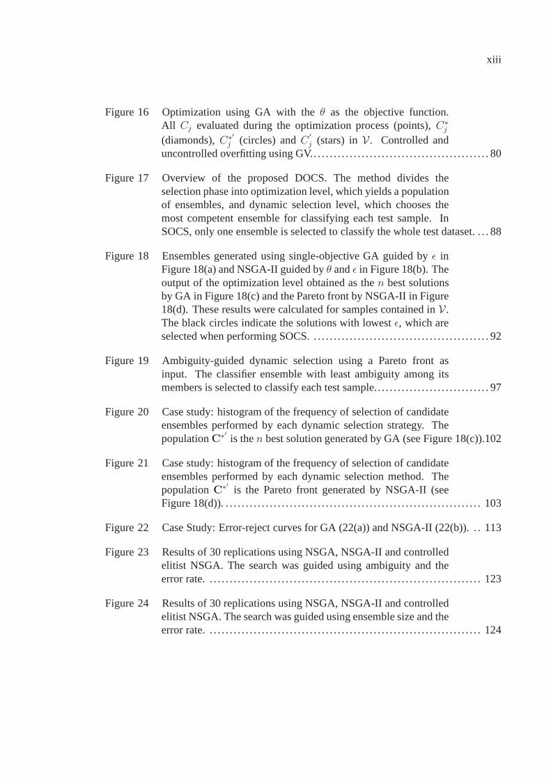
j (stars) inV. Controlled anduncontrolled overfitting using GV.. . . . . . . . . . . . . . . . . . . . .. . . . . . . . . . . . . . . . . . . . . . . 80

Figure 17 Overview of the proposed DOCS. The method divides theselection phase into optimization level, which yields a populationof ensembles, and dynamic selection level, which chooses themost competent ensemble for classifying each test sample. InSOCS, only one ensemble is selected to classify the whole test dataset. . . . 88

Figure 18 Ensembles generated using single-objective GA guided by ǫ inFigure 18(a) and NSGA-II guided byθ andǫ in Figure 18(b). Theoutput of the optimization level obtained as then best solutionsby GA in Figure 18(c) and the Pareto front by NSGA-II in Figure18(d). These results were calculated for samples containedin V.The black circles indicate the solutions with lowestǫ, which areselected when performing SOCS. . . . . . . . . . . . . . . . . . . . . . . . .. . . . . . . . . . . . . . . . . . . . 92

Figure 19 Ambiguity-guided dynamic selection using a Pareto front asinput. The classifier ensemble with least ambiguity among itsmembers is selected to classify each test sample.. . . . . . . . .. . . . . . . . . . . . . . . . . . . 97

Figure 20 Case study: histogram of the frequency of selection of candidateensembles performed by each dynamic selection strategy. ThepopulationC∗′ is then best solution generated by GA (see Figure 18(c)).102

Figure 21 Case study: histogram of the frequency of selection of candidateensembles performed by each dynamic selection method. ThepopulationC

∗′ is the Pareto front generated by NSGA-II (seeFigure 18(d)). . . . . . . . . . . . . . . . . . . . . . . . . . . . . . . . . . . . . . .. . . . . . . . . . . . . . . . . . . . . . . . . . 103

Figure 22 Case Study: Error-reject curves for GA (22(a)) andNSGA-II (22(b)). . . 113

Figure 23 Results of 30 replications using NSGA, NSGA-II andcontrolledelitist NSGA. The search was guided using ambiguity and theerror rate. . . . . . . . . . . . . . . . . . . . . . . . . . . . . . . . . . . . . . . . . .. . . . . . . . . . . . . . . . . . . . . . . . . . . 123

Figure 24 Results of 30 replications using NSGA, NSGA-II andcontrolledelitist NSGA. The search was guided using ensemble size and theerror rate. . . . . . . . . . . . . . . . . . . . . . . . . . . . . . . . . . . . . . . . . .. . . . . . . . . . . . . . . . . . . . . . . . . . . 124

xiv

Figure 25 Uncontrolled overfittingφ based on 30 replications usingGA with diversity measures as the objective function. Theperformances were calculated on the data-test1. The relationshipbetween diversity and error rate becomes stronger asφ decreases. . . . . . . . 128

Figure 26 Uncontrolled overfittingφ based on 30 replications usingGA with diversity measures as the objective function. Theperformances were calculated on the data-test2. The relationshipbetween diversity and error rate becomes stronger asφ decreases. . . . . . . . 129

Figure 27 Pareto front after 1000 generations found using NSGA-II andthe pairs of objective functions: jointly minimize the error rateand the difficulty measure (a), jointly minimize the error rateand ensemble size (b), jointly minimize ensemble size and thedifficulty measure (c) and jointly minimize ensemble size and theinterrater agreement (d). . . . . . . . . . . . . . . . . . . . . . . . . . . . .. . . . . . . . . . . . . . . . . . . . . . . . 133

Figure 28 Scaled objective space of a two-objective problemused tocalculate the overall Pareto spread and thekth objective Paretospread. . . . . . . . . . . . . . . . . . . . . . . . . . . . . . . . . . . . . . . . . . . . .. . . . . . . . . . . . . . . . . . . . . . . . . . . 134

Figure 29 Pareto front after 1000 generations found using NSGA-II andthe pairs of objective functions: minimize ensemble sizeand maximize ambiguity (a) and minimize ensemble size andmaximize Kohavi-Wolpert (b). . . . . . . . . . . . . . . . . . . . . . . . . .. . . . . . . . . . . . . . . . . . . . 139

Figure 30 Optimization using GA guided byǫ. Here, we follow theevolution ofC∗

j (g) (diamonds) forg = 1 (Figure 30(a)) on theoptimization datasetO, as well as on the validation datasetV(Figure 30(b)). Solutions not yet evaluated are in grey and thebest performing solutions are highlighted by arrows. . . . . .. . . . . . . . . . . . . . . . 141

Figure 31 Optimization using GA guided byǫ. Here, we follow theevolution ofC∗

j (g) (diamonds) forg = 52 (Figure 31(a)) on theoptimization datasetO, as well as on the validation datasetV(Figure 31(b)). The minimal error is reached slightly afterg = 52onV, and overfitting is measured by comparing it to the minimalerror reached onO. Solutions not yet evaluated are in grey andthe best performing solutions are highlighted by arrows. . .. . . . . . . . . . . . . . . 142

Figure 32 Optimization using GA guided byǫ. Here, we follow theevolution ofC∗

j (g) (diamonds) formax(g) (Figure 32(a)) on theoptimization datasetO, as well as on the validation datasetV

xv

(Figure 32(b)). The overfitting is measured as the difference inerror betweenC∗′

j (circles) andC∗j (32(b)). There is a 0.30%

overfit in this example. Solutions not yet evaluated are in greyand the best performing solutions are highlighted by arrows. . . . . . . . . . . . . . 142

Figure 33 Optimization using NSGA-II and the pair of objective functions:difficulty measure andǫ. We follow the evolution ofCk(g)(diamonds) forg = 1 (Figure 33(a)) on the optimization datasetO, as well as on the validation datasetV (Figure 33(b)). Solutionsnot yet evaluated are in grey. . . . . . . . . . . . . . . . . . . . . . . . . . .. . . . . . . . . . . . . . . . . . . . . . 143

Figure 34 Optimization using NSGA-II and the pair of objective functions:difficulty measure andǫ. We follow the evolution ofCk(g)(diamonds) forg = 15 (Figure 34(a)) on the optimization datasetO, as well as on the validation datasetV (Figure 34(b)). Theminimal error is reached slightly afterg = 15 on V, andoverfitting is measured by comparing it to the minimal errorreached onO. Solutions not yet evaluated are in grey. . . . . . . . . . . . . . . . .. . . . 143

Figure 35 Optimization using NSGA-II and the pair of objective functions:difficulty measure andǫ. We follow the evolution ofCk(g)(diamonds) formax(g) (Figure 35(a)) on the optimization datasetO, as well as on the validation datasetV (Figure 35(b)). Theoverfitting is measured as the difference in error between the mostaccurate solution inC∗′

k (circles) and inC∗k (35(b)). There is a

0.20% overfit in this example. Solutions not yet evaluated are in grey. . . 144

Figure 36 NIST-digits: the convergence points of GA and PSO.Thegeneration when the best solution was found on optimization(36(a)) and on validation (36(b)). . . . . . . . . . . . . . . . . . . . . .. . . . . . . . . . . . . . . . . . . . . 148

Figure 37 NIST-letters: the convergence points of GA and PSO. Thegeneration when the best solution was found on optimization(37(a)) and on validation (37(b)). . . . . . . . . . . . . . . . . . . . . .. . . . . . . . . . . . . . . . . . . . . 149

Figure 38 NIST-digits: error rates of the solutions found on30 replicationsusing GA and PSO. The performances were calculated on thedata-test1 (38(a)) and on the data-test2 (38(b)). . . . . . . . .. . . . . . . . . . . . . . . . . . 150

Figure 39 NIST-letters: error rates of the solutions found on 30 replicationsusing GA and PSO (39(a)). Size of the ensembles found usingboth GA and PSO search algorithms (39(b)). . . . . . . . . . . . . . . .. . . . . . . . . . . . . . 150

xvi

Figure 40 NIST-digits: Size of the ensembles found using both GA andPSO search algorithms. . . . . . . . . . . . . . . . . . . . . . . . . . . . . . . .. . . . . . . . . . . . . . . . . . . . . . 151

LIST OF ABBREVIATIONS

ADS Ambiguity-guided dynamic selection

BAG Bagging

BKS Behavior-Knowledge Space

BS Backward search

BV Backwarding validation

CSDS Class strength-based dynamic selection

DCS-LA Dynamic classifier selection with local accuracy

DCS Dynamic classifier selection

DOCS Dynamic overproduce-and-choose strategy

DT Decision tree

FS Forward search

FSS Feature subset selection

GA Genetic algorithm

GANSEN GA-based Selective Ensemble

GP Genetic Programming

GV Global Validation

HC Hill-climbing search

Het Heterogeneous classifiers

xviii

IPS kth Objective Pareto Spread

kNN K Nearest Neighbors

KNORA K nearest-oracles

MDS Margin-based dynamic selection

MLP Multilayer perceptron

MOGA Multi-objective genetic algorithm

MOOP Multi-objective optimization problems

NIST National Institute of Standards and Technology

NSGA-II Fast elitist non-dominated sorting genetic algorithm

NSGA Non-dominated Sorting Genetic Algorithm

OCS Overproduce-and-choose strategy

OPS Overall Pareto spread

PBIL Population-based incremental learning

PSO Particle Swarm Optimization

PV Partial Validation

RBF Radial Basis Function

RSS Random subspace method

SOCS Static overproduce-and-choose strategy

SVM Support Vector Machines

TS Tabu search

LIST OF SYMBOLS

ai Ambiguity of thei-th classifier

A Auxiliary archive

αCjLocal candidate ensemble’s class accuracy

C Initial pool of classifiers

C∗′ Population of candidate ensembles found using the validation dataset at

the optimization level

C∗ Population of candidate ensembles found using the optimization dataset

at the optimization level

Cq(g) Offspring population

Cr(g) Elitism population

C(g) Population of ensembles found at each generationg

c∗i Winning individual classifier

ci Individual classifier

C∗′j The best performing subset of classifiers obtained in the validation

dataset

C∗j The best performing subset of classifiers obtained in the optimization

dataset

Cj Individual candidate ensemble

C′

j Candidate ensemble with lowestǫ

xx

Ck(g) Pareto front found inO at generationg

C∗k Final Pareto fronts found inO

C∗′

k Final Pareto fronts found inV

cov Coverage function

δ Double-fault

ǫ The error rate objective function

F Number of classifiers inCj that correctly classify a patternx

f(x) Unknown function

φ Uncontrolled overfitting

G Test dataset

g Each generation step

γ Ambiguity

γ Local ambiguity calculated for the test samplexi,g

h Approximation function

H Hypothesis space

imp Pareto improvement measure

η Disagreement

κ Interrater agreement

l Number of classifiers in candidate ensembleCj

λ Fault majority

xxi

max Maximum rule

max(g) Maximum number of generations

min Minimum rule

mv Majority voting combination function

m(xi) Number of classifiers making error on observationxi

µ Measure of margin

Nab Number of examples classified inX, a, b may assume the value of1

when the classifier is correct and0, otherwise.

n Size of initial pool of candidate classifiers

nb Naive Bayes

O Optimization dataset

P(C) Powerset ofC

p(i) Probability thati classifier(s) fail when classifying a samplex

pr Product rule

p Average individual accuracy

Φ Q-statistic

θ Difficulty measure

Θ Strength relative to the closest class

R∗j Winning region of competence

Rj Regions of competence

xxii

r(x) Number of classifiers that correctly classify samplex

ρ Correlation coefficient

sr Sum rule

σ Coincident failure diversity

T Training dataset

τ Generalized diversity

Ω = ω1, ω2 . . . , ωc Set of class labels

ωk Class labels

V Validation dataset

v(ωk) Number of votes for classωk

w Size of the population of candidate ensembles

ξ Entropy

xi,g Test sample

xi,o Optimization sample

xi,t Training sample

xi,v Validation sample

yi Class label output of thei-th classifier

Y Proportion of classifiers that do not correctly classify a randomly chosen

samplex

ψ Kohavi-Wolpert

ζ Ensemble size

INTRODUCTION

The ensemble of classifiers method has become a dominant approach in several different

fields of application such as Machine Learning and Pattern Recognition. Such interest is

motivated by the theoretical [16] and experimental [31; 96]studies, which show that clas-

sifier ensembles may improve traditional single classifiers. Among the various ensemble

generation methods available, the most popular are bagging[5], boosting [21] and the ran-

dom subspace method [32]. Two main approaches for the designof classifier ensembles

are clearly defined in the literature: (1) classifier fusion;and (2) classifier selection.

The most common and most general operation is the combination of all classifiers mem-

bers’ decisions. Majority voting, sum, product, maximum, minimum [35], Bayesian rule

[86] and Dempster-Shafer [68] are examples of functions used to combine ensemble mem-

bers’ decisions. Classifier fusion relies on the assumptionthat all ensemble members

make independent errors. Thus, pooling the decisions of theensemble members may lead

to increasing the overall performance of the system. However, it is difficult to impose

independence among ensemble’s component members, especially since the component

classifiers are redundant [78], i.e. they provide responsesto the same problem [30]. As

a consequence, there is no guarantee that a particular ensemble combination method will

achieve error independence. When the condition of independence is not verified, it cannot

be guaranteed that the combination of classifier members’ decision will improve the final

classification performance.

Classifier selection is traditionally defined as a strategy which assumes that each ensemble

member is an expert in some local regions of the feature space[107]. The most locally

accurate classifier is selected to estimate the class of eachparticular test pattern. Two cate-

gories of classifier selection techniques exist: static anddynamic. In the first case, regions

of competence are defined during the training phase, while inthe second case, they are

defined during the classification phase taking into account the characteristics of the sam-

2

ple to be classified. However, there may be a drawback to both selection strategies: when

the local expert does not classify the test pattern correctly, there is no way to avoid the

misclassification [80]. Moreover, these approaches, for instanceDynamic Classifier Se-

lection with Local Accuracy(DCS-LA) [101], often involve high computing complexity,

as a result of estimating regions of competence, and may be critically affected by parame-

ters such as the number of neighbors considered (k value) for regions defined by k nearest

neighbors and distance functions.

Another definition of static classifier selection can be found in the Neural Network liter-

ature. It is called either theoverproduce-and-choose strategy[58] or thetest-and-select

methodology[78]. From this different perspective, the overproductionphase involves the

generation of an initial large pool of candidate classifiers, while the selection phase is in-

tended to test different subsets in order to select the best performing subset of classifiers,

which is then used to classify the whole test set. The assumption behind overproduce-and-

choose strategy is that candidate classifiers are redundantas an analogy with the feature

subset selection problem. Thus, finding the most relevant subset of classifiers is better

than combining all the available classifiers.

Problem Statement

In this thesis, the focus is on the overproduce-and-choose strategy, which is traditionally

divided into two phases: (1) overproduction; and (2) selection. The former is devoted to

constructing an initial large pool of classifiers. The latter tests different combinations of

these classifiers in order to identify the optimal candidateensemble. Clearly, the over-

production phase may be undertaken using any ensemble generation method and base

classifier model. The selection phase, however, is the fundamental issue in overproduce-

and-choose strategy, since it focuses on finding the subset of classifiers with optimal accu-

racy. This remains an open problem in the literature. Although the search for the optimal

subset of classifiers can be exhaustive [78], search algorithms might be used when a large

3

initial pool of candidate classifiersC is involved due to the exponential complexity of an

exhaustive search, since the size ofP(C) is 2n, n being the number of classifiers inC and

P(C) the powerset ofC defining the population of all possible candidate ensembles.

When dealing with the selection phase using a non-exhaustive search, two important as-

pects should be analyzed: (1) the search criterion; and (2) the search algorithm. The

first aspect has received a great deal of attention in the recent literature, without much

consensus. Ensemble combination performance, ensemble size and diversity measures

are the most frequent search criteria employed in the literature. Performance is the most

obvious of these, since it allows the main objective of pattern recognition, i.e. finding

predictors with a high recognition rate, to be achieved. Ensemble size is interesting due

to the possibility of increasing performance while minimizing the number of classifiers in

order to accomplish requirements of high performance and low ensemble size [62]. Fi-

nally, there is agreement on the important role played by diversity since ensembles can be

more accurate than individual classifiers only when classifier members present diversity

among themselves. Nonetheless, the relationship between diversity measures and accu-

racy is unclear [44]. The combination of performance and diversity as search criteria in a

multi-objective optimization approach offers a better wayto overcome such an apparent

dilemma by allowing the simultaneous use of both measures.

In terms of search algorithms, several algorithms have beenapplied in the literature for

the selection phase, ranging from ranking then best classifiers [58] togenetic algorithms

(GAs) [70]. GAs are attractive since they allow the fairly easy implementation of en-

semble classifier selection tasks as optimization processes [82] using both single- and

multi-objective functions. Moreover, population-based GAs are good for classifier selec-

tion problems because of the possibility of dealing with a population of solutions rather

than only one, which can be important in performing a post-processing phase. However it

has been shown that such stochastic search algorithms when used in conjunction to Ma-

chine Learning techniques are prone to overfitting in different application problems like

4

the distribution estimation algorithms [102], the design of evolutionary multi-objective

learning system [46], multi-objective pattern classification [3], multi-objective optimiza-

tion of Support Vector Machines [87] and wrapper-based feature subset selection [47; 22].

Even though different aspects have been addressed in works that investigate overfitting

in the context of ensemble of classifiers, for instance regularization terms [63] and meth-

ods for tuning classifiers members [59], very few work has been devoted to the control of

overfitting at the selection phase.

Besides search criterion and search algorithm, other difficulties are concerned when per-

forming selection of classifier ensembles. Classical overproduce-and-choose strategy is

subject to two main problems. First, a fixed subset of classifiers defined using a train-

ing/optimization dataset may not be well adapted for the whole test set. This problem is

similar to searching for a universal best individual classifier, i.e. due to differences among

samples, there is no individual classifier that is perfectlyadapted for every test sample.

Moreover, as stated by the “No Free Lunch” theorem [10], no algorithm may be assumed

to be better than any other algorithm when averaged over all possible classes of problems.

The second problem occurs when Pareto-based algorithms areused at the selection phase.

These algorithms are efficient tools for overproduce-and-choose strategy due to their ca-

pacity to solvemulti-objective optimization problems(MOOPs) such as the simultaneous

use of diversity and classification performance as the objective functions. They use Pareto

dominance to solve MOOPs. Since a Pareto front is a set of nondominated solutions rep-

resenting different tradeoffs with respect to the multipleobjective functions, the task of

selecting the best subset of classifiers is more complex. This is a persistent problem in

MOOPs applications. Often, only one objective function is taken into account to perform

the choice. In [89], for example, the solution with the highest classification performance

was picked up to classify the test samples, even though the solutions were optimized re-

garding both diversity and classification performance measures.

5

Goals of the Research and Contributions

The first goal of this thesis is to determine the best objective function for finding high-

performance classifier ensembles at the selection phase, when this selection is formulated

as an optimization problem performed by both single- and multi-objective GAs. Sev-

eral issues were addressed in order to deal with this problem: (1) the error rate and di-

versity measures were directly compared using a single-objective optimization approach

performed by GA. This direct comparison allowed us to verifythe possibility of using di-

versity instead of performance to find high-performance subset of classifiers. (2) diversity

measures were applied in combination with the error rate in pairs of objective functions in

a multi-optimization approach performed bymulti-objectiveGA (MOGA) in order to in-

vestigate whether including both performance and diversity as objective functions leads to

selection of high-performance classifier ensembles. Finally, (3) we investigated the possi-

bility of establishing an analogy between feature subset selection and ensemble classifier

selection by combining ensemble size with the error rate, aswell as with the diversity

measures in pairs of objective functions in the multi-optimization approach. Part of this

analysis was presented in [72].

The second goal is to show experimentally that an overfittingcontrol strategy must be

conductedduring the optimization process, which is performed at the selection phase. In

this study, we used the bagging and random subspace algorithms for ensemble generation

at the overproduction phase. The classification error rate and a set of diversity measures

were applied as search criteria. Since both GA and MOGA search algorithms were exam-

ined, we investigated in this thesis the use of an auxiliary archive to store the best subset

of classifiers (or Pareto front in the MOGA case) obtained in avalidation process using

a validation dataset to control overfitting. Three different strategies to update the aux-

iliary archive have been compared and adapted in this thesisto the context of single and

multi-objective selection of classifier ensembles: (1)partial validationwhere the auxiliary

archive is updated only in the last generation of the optimization process; (2)backward-

6

ing [67] which relies on monitoring the optimization process byupdating the auxiliary

archive with the best solution from each generation and (3)global validation[62] up-

dating the archive by storing in it the Pareto front (or the best solution in the GA case)

identified on the validation dataset at each generation step.

The global validation strategy is presented as a tool to showthe relationship between

diversity and performance, specifically when diversity measures are used to guide GA.

The assumption is that if a strong relationship between diversity and performance exists,

the solution obtained by performing global validation solely guided by diversity should be

close or equal to the solution with the highest performance among all solutions evaluated.

This offers a new possibility to analyze the relationship between diversity and performance

which has received a great deal of attention in the literature. In [75], we present this

overfitting analysis.

Finally, the last goal is to propose a dynamic overproduce-and-choose strategy which com-

bines optimization and dynamic selection in a two-level selection phase to allow selection

of the most confident subset of classifiers to label each test sample individually. Selection

at the optimization level is intended to generate a population of highly accurate candidate

classifier ensembles, while at the dynamic selection level measures of confidence are used

to reveal the candidate ensemble with highest degree of confidence in the current decision.

Three different confidence measures are investigated.

Our objective is to overcome the three drawbacks mentioned above: Rather than select-

ing only one candidate ensemble found during the optimization level, as is done instatic

overproduce-and-choose strategy, the selection of the best candidate ensemble is based

directly on the test patterns. Our assumption is that the generalization performance will

increase, since a population of potential high accuracy candidate ensembles are considered

to select the most competent solution for each test sample. This first point is particularly

important in problems involving Pareto-based algorithms,because our method allows all

7

equally competent solutions over the Pareto front to be tested; (2) Instead of using only

one local expert to classify each test sample, as is done in traditional classifier selec-

tion strategies (both static and dynamic), the selection ofa subset of classifiers may de-

crease misclassification; and, finally, (3) Our dynamic selection avoids estimating regions

of competence and distance measures in selecting the best candidate ensemble for each

test sample, since it relies on calculating confidence measures rather than on performance.

Moreover, we prove both theoretically and experimentally that the selection of the solution

with the highest level of confidence among its members permits an increase in the “degree

of certainty" of the classification, increasing the generalization performance as a conse-

quence. These interesting results motivated us to investigate three confidence measures in

this thesis which measure the extent of consensus of candidate ensembles: (1)Ambiguity

measures the number of classifiers in disagreement with the majority voting; (2)Margin,

inspired by the definition of margin, measures the difference between the number of votes

assigned to the two classes with the highest number of votes,indicating the candidate en-

semble’s level of certainty about the majority voting class; and (3)Strength relative to the

closest class[8] also measures the difference between the number of votesreceived by

the majority voting class and the class with the second highest number of votes; however,

this difference is divided by the performance achieved by each candidate ensemble when

assigning the majority voting class for samples contained in a validation dataset. This ad-

ditional information indicates how often each candidate ensemble made the right decision

in assigning the selected class.

As marginal contributions, we also point out the best methodfor the overproduction phase

on comparing bagging and the random subspace method. In [73], we first introduced the

idea that choosing the candidate ensemble with the largest consensus, measured using

ambiguity, to predict the test pattern class leads to selecting the solution with greatest

certainty in the current decision. In [74], we present the complete dynamic overproduce-

and-choose strategy.

8

Organization of the Thesis

This thesis is organized as follows. In Chapter 1, we presenta brief overview of the liter-

ature related to ensemble of classifiers in order to be able tointroduce all definitions and

research work related to the overproduce-and-choose strategy. Firstly, the combination of

classifier ensemble is presented. Then, the traditional definition of dynamic classifier se-

lection is summarized. Finally, the overproduce-and-choose strategy is explained. In this

chapter we emphasize that the overproduce-and-choose strategy is based on combining

classifier selection and fusion. In addition, it is shown that the overproduce-and-choose

strategies reported in the literature are static selectionapproaches.

In Chapter 2, we investigate the search algorithm and searchcriteria at the selection phase,

when this selection is performed as an optimization process. Single- and multi-objective

GAs are used to conduct the optimization process, while fourteen objective functions are

used to guide this optimization. Thus, the experiments and the results are presented and

analyzed.

The overfitting aspect is addressed in Chapter 3. We demonstrate the circumstances under

which the process of classifier ensemble selection results in overfitting. Then, three strate-

gies used to control overfitting are introduced. Finally, experimental results are presented.

In Chapter 4 we present our proposed dynamic overproduce-and-choose strategy. We

describe the optimization and the dynamic selection levelsperformed in the two-level

selection phase by population-based GAs and confidence-based measures respectively.

Then, the experiments and the results obtained are presented. Finally, our conclusions and

suggestions for future work are discussed.

CHAPTER 1

LITERATURE REVIEW

Learning algorithms are used to solve tasks for which the design of software using tra-

ditional programming techniques is difficult. Machine failures prediction, filter for elec-

tronic mail messages and handwritten digits recognition are examples of these tasks. Sev-

eral different learning algorithms have been proposed in the literature such as Decision

Trees, Neural Networks,k Nearest Neighbors (kNN), Support Vector Machines (SVM),

etc. Given samplex and its class labelωk with an unknown functionωk = f(x), all these

learning algorithms focus on finding in the hypothesis spaceH the best approximation

functionh, which is a classifier, to the functionf(x). Hence, the goal of these learning

algorithms is the design of a robust well-suited single classifier to the problem concerned.

Classifier ensembles attempt to overcome the complex task ofdesigning a robust, well-

suited individual classifier by combining the decisions of relatively simpler classifiers. It

has been shown that significant performance improvements can be obtained by creating

classifier ensembles and combining their classifier members’ outputs instead of using sin-

gle classifiers. Altinçay [2] and Tremblay et al. [89] showedthat ensemble of kNN is

superior to single kNN; Zhang [105] and Valentini [93] concluded that ensemble of SVM

outperforms single SVM and Ruta and Gabrys [71] demonstrated performance improve-

ments by combining ensemble of Neural Networks, instead of using a single Neural Net-

work. Moreover, the wide applicability of ensemble-of-classifier techniques is important,

since most of the learning techniques available in the literature may be used for generat-

ing classifier ensembles. Besides, ensembles are effectivetools to solve difficulty Pattern

Recognition problems such as remote sensing, person recognition, intrusion detection,

medical applications and others [54].

10

According to Dietterich [16] there are three main reasons for the improved performance

verified using classifier ensembles: (1)statistical; (2) computational; and (3)representa-

tional. Figure 1 illustrates these reasons. The first aspect is related to the problem that

arises when a learning algorithm finds different hypotheseshi, which appear equally ac-

curate during the training phase, but chooses the less competent hypothesis, when tested

in unknown data. This problem may be avoided by combining allclassifiers. The compu-

tational reason refers to the situation when learning algorithms get stuck in local optima,

since the combination of different local minima may lead to better solutions. The last

reason refers to the situation when the hypothesis spaceH does not contain good approx-

imations to the functionf(x). In this case, classifier ensembles allow to expand the space

of functions evaluated, leading to a better approximation of f(x).

Figure 1 The statistical, computational and representational reasons for combiningclassifiers [16].

11

However, the literature has shown that diversity is the key issue for employing classifier

ensembles successfully [44]. It is intuitively accepted that ensemble members must be dif-

ferent from each other, exhibiting especially diverse errors [7]. However, highly accurate

and reliable classification is required in practical machine learning and pattern recognition

applications. Thus, ideally, ensemble classifier members must be accurate and different

from each other to ensure performance improvement. Therefore, the key challenge for

classifier ensemble research is to understand and measure diversity in order to establish

the perfect trade-off between diversity and accuracy [23].

Although the concept of diversity is still considered an ill-defined concept [7], there are

several different measures of diversity reported in the literature from different fields of re-

search. Moreover, the most widely used ensemble creation techniques, bagging, boosting

and the random subspace method are focused on incorporatingthe concept of diversity

into the construction of effective ensembles. Bagging and the random subspace method

implicitly try to create diverse ensemble members by using random samples or random

features respectively, to train each classifier, while boosting try to explicitly ensure diver-

sity among classifiers. The overproduce-and-choose strategy is another way to explicitly

enforce a measure of diversity during the generation of ensembles. This strategy allows

the selection of accurate and diverse classifier members [69].

This chapter is organized as follows. In section 1.1, it is presented a survey of construction

of classifier ensembles. Ensemble creation methods are described in section 1.1.1, while

the combination functions are discussed in section 1.1.2. In section 1.2 it is presented an

overview of classifier selection. The classical dynamic classifier selection is discussed in

section 1.2.1; the overproduce-and-choose strategy is presented in section 1.2.2; and the

problem of overfitting in overproduce-and-choose strategyis analysed in section 1.2.3.

Finally, section 1.3 presents the dicussion.

12

1.1 Construction of classifier ensembles

The construction of classifier ensembles may be performed byadopting different strate-

gies. One possibility is to manipulate the classifier modelsinvolved, such as using different

classifier types [70], different classifier architectures [71] and different learning parame-

ters initialization [2]. Another option is varying the data, for instance using different data

sources, different pre-processing methods, different sampling methods, distortion, etc. It

is important to mention that the generation of an ensemble ofclassifiers involves the de-

sign of the classifiers members and the choice of the fusion function to combine their

decisions. These two aspects are analyzed in this section.

1.1.1 Strategies for generating classifier ensembles

Some authors [77; 7] have proposed to divide the ensemble creation methods into different

categories. Sharkey [77] have shown that the following fouraspects can be manipulated

to yield ensembles of Neural Networks: initial conditions,training data, topology of the

networks and the training algorithm. More recently, Brown et. al. [7] proposed that

ensemble creation methods may be divided into three groups according to the aspects

that are manipulated. (1)Starting point in hypothesis spaceinvolves varying the start

points of the classifiers, such as the initial random weightsof Neural Networks. (2)Set of

accessible hypothesisis related to varying the topology of the classifiers or the data, used

for training ensemble’s component members. Finally, (3)traversal of hypothesis spaceis

focused on enlarging the search space in order to evaluate a large amount of hypothesis

using genetic algorithms and penalty methods, for example.We present in this section the

main ensemble creation methods divided into five groups. This categorization takes into

account whether or not one of the following aspects are manipulated: training examples,

input features, output targets, ensemble members and injecting randomness.

13

Manipulating the Training Examples

This first group contains methods, which construct classifier ensembles by varying the

training samples in order to generate different datasets for training the ensemble members.

The following ensemble construction methods are examples of this kind of approach.

• Bagging - It is a bootstrap technique proposed by Breiman [5]. Bagging is an

acronym forBootstrapAggregation Learning, which buildsn replicate training

datasets by randomly sampling, with replacement, from the original training dataset.

Thus, each replicated dataset is used to train one classifiermember. The classifiers

outputs are then combined via an appropriate fusion function. It is expected that

63,2% of the original training samples will be included in each replicate [5].

• Boosting- Several variants of boosting have been proposed. We describe here the

Adaboost (short forAdaptiveBoosting) algorithm proposed by Freund and Schapire

[21], which appears to be the most popular boosting variant [54]. This ensemble

creation method is similar to bagging, since it also manipulates the training exam-

ples to generate multiple hypotheses. However, boosting isan iterative algorithm,

which assigns weights to each example contained in the training dataset and gener-

ates classifiers sequentially. At each iteration, the algorithm adjusts the weights of

the misclassified training samples by previous classifiers.Thus, the samples consid-

ered by previous classifiers as difficult for classification,will have higher chances

to be put together to form the training set for future classifiers. The final ensem-

ble composed of all classifiers generated at each iteration is usually combined by

majority voting or weighted voting.

• Ensemble Clustering- It is a method used in unsupervised classification that is moti-

vated for the success of classifier ensembles in the supervised classification context.

The idea is to use a partition generation process to produce different clusters. Af-

terwards, these partitions are combined in order to producean improved solution.

14

Diversity among clusters is also important for the success of this ensemble creation

method and several strategies to provide diversity in cluster algorithms have been

investigated [26].

It is important to take into account the distinction betweenunstableor stableclassifiers

[42]. The first group is strongly dependent on the training samples, while the second group

is less sensitive to changes on the training dataset. The literature has shown that unstable

classifiers, such as Decision Trees and Neural Networks, present high variance, which is a

component of the bias-variance decomposition of the error framework [19]. Consequently,

stable classifiers like kNN and Fischer linear discriminantpresent low variance. Indeed,

one of the advantages of combining individual classifiers tocompose one ensemble is

to reduce the variance component of the error [59]. Thus, dueto the fact that boosting

is assumed to reduce both bias and variance [19], this ensemble generation method is

efficient using both stable and unstable classifiers. On the other hand, bagging is mostly

effective with unstable classifiers, since bagging is assumed to reduce variance [94].

Manipulating the Input Features

These methods construct classifier ensembles manipulatingthe original set of features

available for training. The objective is to provide a partial view of the training dataset to

each ensemble member, leading them to be different from eachother. In addition, these

methods try to reduce the number of features to fight the effects of the so-calledcurse of

dimensionalityproblem [90].

• Feature Subset Selection- The objective of ensemble feature selection is to build sets

of classifiers using small subsets of features whilst keeping high accurate classifiers,

as was done in [51]. An interesting overview about several techniques used to create

ensemble feature selection is presented in [90].

15

• The Random Subspace Method- This method introduced by Ho in [32] is considered

to be a feature subset selection approach. It works by randomly choosingn different

subspaces from the original feature space. Each random subspace is used to train

one individual classifier. Then classifiers are usually combined by the majority

voting rule. Although the random subspace method is supposed to reduce variance

[94], it is assumed be an efficient method for building ensembles using both stable

and unstable classifiers.

Manipulating the Output Targets

This group contains methods, which are based on manipulating the labels of the samples

contained in the training dataset. In the error-correctingoutput coding technique used

by Dietterich and Bakiri [18], a multi-class problem is transformed into a set of binary

problems. At each iteration a new binary division of the training dataset is used to train a

new classifier. Another example is the method proposed by Breiman [6], which introduces

noise to change some class labels of the training samples.

Manipulating the Ensemble Members (Heterogeneous Ensembles)

These methods work by using different classifier types [70],different classifier architec-

tures [69] or different initializations of the learning parameters [107], whilst maintaining

the same training dataset. For instance, Valentini and Dietterich [95] used an ensemble

of SVM with kernel RBF (radial basis functions) in which the classifier members were

trained using different parametersσ. Ruta and Gabrys [70] employed 15 different learn-

ing algorithms, including Quadratic discriminant, RadialBasis Network, k-NN, Decision

Tree, and others, in order to compose an ensemble of 15 heterogeneous classifiers.

16

Injecting randomness

This group contains methods, which inject randomness into the classifier members to pro-

duce different classifiers in order to build ensembles. The random initial weights of Neural

Networks [78] and the random choice of the feature that decides the split at the internal

nodes of Decision Tree [17], are examples of randomness injected into classifier members.

1.1.2 Combination Function

The application of one of the above mentioned ensemble creation methods generates an

initial set of classifiersC, whereC = c1, c2, . . . , cn. Figure 2 shows that the ensem-

ble generation method is employed using samplesxi,t contained in the training dataset

T . Given such a pool of classifiers, the most common operation is the fusion of alln

classifiers. Thus, an effective way of combining the classifier members’ outputs must

be found. Even though some classification techniques, such as Neural Networks [97] and

Polynomial classifiers [20], have been used to combine classifier members, there are many

different classifier fusion functions proposed. In this section we present a brief description

of some of the most widely used fusion functions.

EnsembleGeneration

Method

T

xi,t

C = c1, c2, . . . , cn

Figure 2 Overview of the creation process of classifier ensembles.

17

Majority Voting

It is the simplest and most popular method to combine classifiers. The definition presented

in Equation 1.1 is also calledPlurality vote[40]. Considering the set ofn classifiers,yi as

the class label output of thei-th classifier, and a classification problem with the following

set of class labelsΩ = ω1, ω2 . . . , ωc, majority voting for samplex is calculated as:

mv(x) = maxck=1

n∑

i=1

yi,k (1.1)

When there is a tie for the number of votes, it may be broken randomly or a rejection strat-

egy must be performed. There are other versions of vote, suchas unanimous consensus,

weighted voting, etc [40].

Product Rule

It is a simple combination function that is calculated taking into account outputs of classi-

fiersci provided as class probabilitiesP (ωk|yi(x)), denoting that the class label of sample

x is ωk if classifierci assigns the class label outputyi. The product rule is computed as:

pr(x) = maxck=1

n∏

i=1

P (ωk|yi(x)) (1.2)

Sum Rule

This function also operates using the class probabilities provided by classifier membersci.

The decision is obtained as follows:

sr(x) = maxck=1

n∑

i=1

P (ωk|yi(x)) (1.3)

18

Maximum Rule

It is possible to approximate the combination functions product (Equation 1.2) and sum

(Equation 1.3) by its upper or lower bounds. If the sum is approximated by the maximum

of the class probabilities, max rule is obtained as:

max(x) = maxck=1maxni=1P (ωk|yi(x)) (1.4)

Minimum Rule

This function is obtained through approximating the product rule of class probabilities by

the minimum:

min(x) = maxck=1minni=1P (ωk|yi(x)) (1.5)

Naive Bayes

This method, also called Bayesian combination rule [86], assumes that classifier members

are mutually independent and operates on the confusion matrix of each classifier member

ci. The objective is to take into account the performance of each classifierci, for each

class involved in the classification problem, over samples contained in datasetT . Let

P (ωt|yi(x) = ωk) be an estimated of the probability that the true class label of samplex

is ωt if classifierci assigns as output the class labelωk. The probabilityP (ωt|yi(x) = ωk)

is computed as the ratio between the number of training samples assigned by classifier

ci to classωk, whose true class label isωt, and the total number of training samples as-

signed byci to classωk. Thus, Naive Bayes classifies new samples using these estimated

probabilities as follows:

nbk(x) =

n∏

i=1

P (ωt|yi(x) = ωk) (1.6)

19

Naive Bayes decision rule selects the class with the highestprobability computed by the

estimated probabilities in Equation 1.6.

Dempster-Shafer

This combination method is based on belief functions. Giventhe set of class labels

Ω = ω1, ω2 . . . , ωc, the setΩ has subsets which are known as propositions. The set

of propositions is denoted asP . LettingA andB denote two arbitrary class sets where

A ∈ P andB ∈ P , a basic probability assignment (bpa) is assigned to each proposition,

for instancebpa(A) represents the output of the classifier onA. Thus, the basic proba-

bilities assigned to all subsets ofA are added in order to calculate a numeric value in the

range[0, 1] that indicates the belief in proposition, as follows:

bel(A) =∑

B⊆A

bpa(A) (1.7)

Given the setsA andB with two different basic probabilities,bpa1(A) for one classifier

andbpa2(B) for the other classifier,C indicates the basic probability of their conjunction

C = A ∩ B, which is proportional tobpa1(A) x bpa2(B). Finally, the classifiers are then

combined by using the Dempster-Shafer rule as:

bpa1 ⊕ bpa2(C) =

∑

A∩B=C bpa1(A)bpa2(B)

1 −∑

A∩B=∅ bpa1(A)bpa2(B)(1.8)

The fusion functions described in this section are few examples of the variety of classifier

combination rules reported in the literature. Other approaches to combine ensemble clas-

sifier members include Behavior-Knowledge Space (BKS) [33], Decision Templates [41]

and Wernecke’s method [98].

Classifier fusion assumes error independence among ensemble’s component members.

This means that the classifier members are supposed to misclassify different patterns [43].

20

In this way, the combination of classifier members’ decisionwill improve the final classi-

fication performance. However, when the condition of independence is no verified, there

is no guarantee that the combination of classifiers will outperform single classifiers [83].

On the one hand, it is difficult to impose independence among ensemble’s component

members. On the other, the selection of classifiers has focused on finding either the most

efficient individual classifier or the best subset of classifiers, rather than combining all

availablen classifiers. Therefore, classifier selection techniques avoid the assumption of

independence. Classifier selection is described in the nextsection.

1.2 Classifier Selection

It was mentioned in the introduction that classifier selection is traditionally defined as a

strategy that assumes each ensemble member as an expert in some regions of competence

[55; 107]. The selection is called dynamic or static whetherthe regions of competence

are defined during the test or the training phase respectively. However, several methods

reported in the literature as dynamic classifier selection methods define regions of com-

petence during the training phase [107; 81; 79]. These strategies are discussed in section

1.2.1. The overproduce-and-choose strategy, which is the classifier ensemble selection

technique studied in this thesis, is classically assumed tobe a static classifier selection

method [69]. In section 1.2.2 we present an overview of the overproduce-and-choose

strategy.

1.2.1 Dynamic Classifier Selection

Classicaldynamic classifier selection(DCS) methods are divided into three levels, as illus-

trated in Figure 3. The first level, calledclassifier generationemploys one of the ensemble

creation methods presented in section 1.1.1, using the samplesxi,g contained in the train-

ing datasetT , to obtain classifiers to compose the initial pool of classifiersC. However,

rather than combining all availablen classifiers using one of the fusion functions men-

tioned in section 1.1.2, the second level calledregion of competence generation, usesT

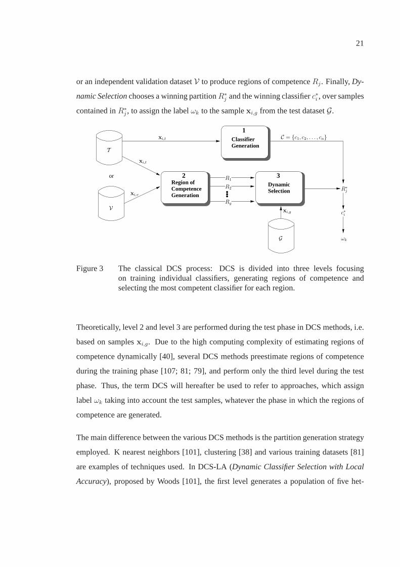
21

or an independent validation datasetV to produce regions of competenceRj . Finally,Dy-

namic Selectionchooses a winning partitionR∗j and the winning classifierc∗i , over samples

contained inR∗j , to assign the labelωk to the samplexi,g from the test datasetG.

Dynamic Selection

or

CompetenceGeneration

Generation

Region of

Classifier

V

3

G

...

T

xi,v

xi,t

xi,g

R∗j

xi,t

R1

R2

Ry

c∗i

ωk

C = c1, c2, . . . , cn

2

1

Figure 3 The classical DCS process: DCS is divided into threelevels focusingon training individual classifiers, generating regions of competence andselecting the most competent classifier for each region.

Theoretically, level 2 and level 3 are performed during the test phase in DCS methods, i.e.

based on samplesxi,g. Due to the high computing complexity of estimating regionsof

competence dynamically [40], several DCS methods preestimate regions of competence

during the training phase [107; 81; 79], and perform only thethird level during the test

phase. Thus, the term DCS will hereafter be used to refer to approaches, which assign

labelωk taking into account the test samples, whatever the phase in which the regions of

competence are generated.

The main difference between the various DCS methods is the partition generation strategy

employed. K nearest neighbors [101], clustering [38] and various training datasets [81]

are examples of techniques used. In DCS-LA (Dynamic Classifier Selection with Local

Accuracy), proposed by Woods [101], the first level generates a population of five het-

22

erogeneous classifiers through feature subset selection. The algorithm defines the local

regionR∗j as the set of k nearest neighbors fromT surroundingxi,g. Thus, at the third

level, the local accuracy of each classifierci is estimated, and the most locally accurate

classifierc∗i is then selected to estimate the true class ofxi,g. Giacinto and Roli [24] pro-

posed an approach very similar to Woods’ method. The difference is that the local region

used to estimate the individual performances of eachci is defined as the nearest neighbors

from V that have a similarity withxi,g that is higher than a threshold. Such a similarity

is measured by comparing the vector of class labels assignedby eachci to xi,g and to its

neighbors.

In the clustering and selection method proposed by Kuncheva[38], multilayer perceptrons

(MLPs) with different number of nodes in the hidden layer composeC. Thus, at the second

level, the feature space is partitioned into clusters usingK means, and cluster centroids are

computed. At the third level, the region with a cluster center nearest toxi,g is picked up

asR∗j and theci with the highest classification accuracy is nominated to label xi,g. In the

DCS method employed by Sohn and Shin [85],T is first divided inton clusters, cluster

centroids are computed and each cluster is used to train one classifier. The base algorithm

was a logistic model. The second level and the third level areconducted as in Kuncheva’s

method [38]. Liu et al. [45] presented a clustering and selection-based method that first

generates three heterogeneous classifiers to composeC. At the second level,T is divided

into two groups for eachci: (1) correctly classified training samples; and (2) misclassified

training samples. These two groups are further partitionedusing a clustering algorithm to

compose regions of competence, i.e. eachci has its own. At the dynamic selection level,

the cluster closest toxi,g from each ofci’s regions of competence is pointed out and the

most accurate classifier is chosen to assignxi,g’s label.

Singh and Singh [81] described a DCS method for image region labeling in which the first

level generatesC by training eachci (kNN classifiers) withn different training datasets

which are obtained through applyingn different texture analysis methods. The regions of

23

competence are defined at the second level as the class centroids of each training dataset.

The selection level measures the distance betweenxi,g and all the class centroids. Then,

theci responsible by the closest region is selected to classifyxi,g. In [107], a DCS method

for data stream mining applications is proposed. For the first level, T is divided into

n chunks which are further used to train then DT classifiers that composeC. Local

regions are generated with statistical information on the attribute values of samples from

V. Finally, at the third level, the most accurate classifier inthe region sharing the same

statistical information on attribute values withxi,g is selected to label it.

It is important to mention that all these methods pick up onlyone candidate classifier

to make the decision. This may lead to a classifier with a low level of confidence in its

decision, or even one with a wrong decision, being chosen. A combination of selection

and fusion has been investigated in the literature as a strategy for avoiding this drawback.

Kuncheva [39] proposed to use statistical tests to switch between selection and fusion.

The classifierc∗i , selected using clustering and selection [38], is employedto labelxi,g

only when it is significantly better than the remaining classifiers. Otherwise, all classifiers

in C are combined through decision templates. Gunes et al. [28] applied a fuzzy clustering

algorithm in combination with ambiguity rejection in ordermake it possible to deal with

overlapping regions of competence. They switch between classifyingxi,g using eitherc∗i or

the combination of the best adapted classifiers whetherxi,g falls into a single cluster or into

an ambiguous cluster, respectively. The k-nearest-oracles (KNORA) method proposed

by Ko et al. [36] explores the properties of the oracle concept [15] to select the most

suitable classifier ensemble for each test sample. KNORA first finds the set of k nearest

neighbors fromV surroundingxi,g. Then the algorithm selects each classifierci, which

correctly classifies this set of neighbors, to compose a classifier ensemble. This selected

classifier ensemble is then used for classifyingxi,g. In the method used by Tsymbal et

al. [92], called Dynamic Voting with Selection (DVS), a weight is determined for each

classifierci according to its local accuracy measured using the set of k nearest neighbors

24

from V surroundingxi,g. Then, the classifiers with the lowest accuracy are removed,

while the remaining classifiers are combined through weighted voting to assign the class

of xi,g. Finally, Soares et al. [84] have tailored Kuncheva’s method [39] to select candidate

classifiers based on accuracy and diversity.

Table I

Compilation of some of the results reported in the DCS literature highlighting the type ofbase classifiers, the strategy employed for generating regions of competence, and the

phase in which they are generated, the criteria used to perform the selection and whetheror not fusion is also used (Het: heterogeneous classifiers).

Reference Classifier Regions of Partition Selection SelectionNumber Members Competence Phase Criteria /fusion[107] DT Blocks of samples Training Accuracy Selection[24] Het kNN rule Test Accuracy Selection[101] Het kNN rule Test Accuracy Selection[81] kNN Different features Training Distance measure Selection[38] MLP Clustering Training Distance & accuracy Selection[85] Logistic Clustering Training Distance & accuracy Selection[45] Het Clustering Training Distance & accuracy Selection[39] MLP/Het Clustering Training Distance & accuracy Selection or fusion[28] Bayesian Clustering Training Distance measure Selection or fusion[36] kNN kNN rule Test Oracle Selection & fusion[92] Het kNN rule Test Accuracy Selection & fusion[84] Het Clustering Training Accuracy & diversity Selection & fusion

Table I summarizes the DCS methods reported in the literature and mentioned in this

section. It is interesting to note that heterogeneous classifiers at the first level, clustering

at the second level and accuracy as a selection criterion at the third level are most often

applied. An alternative to DCS is the overproduce-and-choose strategy, which allows the

selection of classifier ensembles instead of only one classifier. Hence, this strategy is also

based on combining selection and fusion, as it is explained in the next section.

25

1.2.2 Overproduce-and-Choose Strategy

Given the pool of classifiersC = c1, c2, . . . , cn generated using any ensemble creation

method, classifier fusion combines then classifiers assuming that they are all important

and independent. By contrast, classifier selection, especially DCS, selects one individual

classifierc∗i to assign the label of each sample contained in the test datasetG. A combina-

tion of both approaches is theoverproduce-and-choose strategy(OCS). The objective of

OCS is to find the most relevant subset of classifiers, based onthe assumption that clas-

sifiers inC are redundant [106]. Once the best subset of classifiers has been selected, the

output of its classifier members must be combined.

Methods based on OCS are divided into two phases: (1)overproduction; and (2)selection.

The first phase is related to the first level of DCS, here however, the overproduction phase

must construct an initiallargepool of candidate classifiersC, using the training datasetT .

The second phase is devoted to identify the best performing subset of classifiers inP(C).

As mentioned in the introduction,P(C) is the powerset ofC defining the population of all

possible candidate ensemblesCj. The selected ensembleC∗j is then combined to estimate

the class labels of the samples contained in the test datasetG. Figure 4 illustrates the OCS

phases.

OCS based in heuristic techniques has been proposed in the literature. Margineantu and

Dietterich [48] proposed an OCS to reduce the computationalcosts of boosting. The

pool C was composed of homogeneous DT generated by boosting. Then,pruning algo-

rithms were applied to select each classifierci used to formC∗j . The authors pointed

out a diversity-based pruning algorithm, which used Kappa diversity, as the best pruning

method. Partridge and Yates [58] generated the poolC using two types of Neural Net-

works, MLP and Radial Basis Function (RBF). The Neural Networks were trained using

different number of hidden units and weight initialization. They proposed the use of two

heuristics during the selection phase. The first heuristic relies on ranking the candidate

26

EnsembleGeneration

Method

OVERPRODUCTION PHASE SELECTION PHASE

T

cn

GC1

C2

Cw

Population

Pool of classifiersC

C∗j

xi,t c2

c1

P(C)

of ensembles

xi,g

ωk

Figure 4 Overview of the OCS process. OCS is divided into the overproductionand the selection phases. The overproduction phase createsa large pool ofclassifiers, while the selection phase focus on finding the most performingsubset of classifiers.

classifiers by its performance and selecting thek best to composeC∗j , wherek < n. The

second heuristic, picks the classifier with the highest performance, from each type of clas-

sifier, to composeC∗j . In the same light, Canuto et al. [9] generatedC using heterogeneous

classifiers such as MLP, RBF, SVM, kNN, and others, and testeddifferent fixed sizes of

classifier ensembles. Their selection phase took into account both performance and diver-

sity of each candidate ensemble generated. Aksela and Laaksonen [1] also generated a

poolC of heterogeneous classifiers at the overproduction phase. Neural Networks, SVM,

etc, are examples of classifiers used. The authors successfully applied an OCS for se-

lecting classifiers focusing on the diversity of errors. Thecandidate ensembles were also

generated using fixed ensembles’ size.

Although these heuristic-based approaches lead to reduce the complexity of the selection

phase, there is no guarantee that the optimal solution will be found. An alternative to

heuristic-based OCS is to use search algorithms. When performing OCS using search

27

algorithms, it is important to choose the best search criterion and the best search algo-

rithm for the classifier ensemble selection problem. Sharkey and Sharkey [78] proposed

an exhaustive search algorithm to findC∗j from an initial poolC composed of MLPs. The

classifiers were trained using different number of hidden units and different random initial

conditions. Thus, candidate ensembles’ performances wereused to guide the selection

phase. Based on the same idea, Zhou et al. [107] developed equations, which were used

to identify the classifiers that should be eliminated fromC in order to keep the combina-

tion with optimal accuracy. Their poolC was composed of different Neural Networks.

Nonetheless, non-exhaustive search algorithms might be used when a largeC is available

due to the high computing complexity of an exhaustive search, since the size ofP(C) is

2n.

Several non-exhaustive search algorithms have been applied in the literature for the selec-

tion of classifier ensembles. Zhou et al. [107] proposed GANSEN (GA-based Selective

Ensemble), which employs GAs to assign random weight to eachNeural Network and

evolves these weights by assessing the performance of the combination obtained when

each Neural Network is included in the ensemble. Then, each Neural Network whose

weight is higher than a fixed threshold is used to composeC∗j . Roli et al. [69] compared

forward (FS), backward (BS) and tabu (TS) search algorithms, guided by accuracy and

the following three diversity measures: generalized diversity (τ ), Q-statistic [44] (Φ) and

double-fault (δ), called by the authors compound diversity. Their initial pool C was com-

posed of heterogeneous classifiers such as MLP, kNN and RBF. They concluded that the

search criteria and the search algorithms investigated presented equivalent results. Follow-

ing the idea of identifying the best search criteria and search algorithm, Ruta and Gabrys

[70], used the candidate ensembles’ error rate and 12 diversity measures, including the

same measures investigated by Roli et al. [69], to guide the following 5 single-objective

search algorithms: FS, BS, GA, stochastic hill-climbing (HC) search and population-based

incremental learning (PBIL). They concluded that diversity was not a better measure for

28

finding ensembles that perform well than the candidate ensembles’ error rate. Their ini-

tial pool of candidate classifiers was composed of 15 heterogeneous classifiers, including

MLP, kNN, RBF, Quadratic Bayes, and others.

The combination of the error rate and diversity as search criteria allows the simultaneous

use of both measures in OCS. It is not surprising that this idea has already been inves-

tigated in the literature. Opitz and Shavlik [53] applied a GA using a single-objective

function combining both the error rate and ambiguity diversity measure (as defined in

[53]) to search forC∗j in a populationC of Neural Networks. They showed that this OCS

outperformed the combination of all classifiers inC. Zenobi and Cunningham [104] cre-

ated at the overproduction phase a poolC of kNN classifiers by applying a feature subset

selection approach. At the selection phase, ambiguity (as defined in [104]) and the error

rate were used to guide a hill-climbing search method. They showed that their combined

approach outperformed the ensembles selected using the error rate as the only objective

function. Tremblay et al. [89] used a MOGA (a modified versionof Non-dominated Sort-

ing GA - NSGA [11]) guided by pairs of objective functions compose of the error rate

with the following four diversity measures: ambiguity [104] (γ), fault majority [70] (λ),

entropy (ξ) and Q-statistic (Φ) [44]. They generated a poolC of kNN classifiers gener-

ated by the random subspace method at the overproduction phase. They concluded that

MOGA did not find better ensembles than single-objective GA using only the error rate

as the objective function. Finally, in the OCS proposed by Oliveira et al. [51], a feature

subset selection process was applied to generate a population of Neural Networks at the

overproduction phase. The selection phase was also guided by γ and the error rate as the

objective functions.

It is important to mention that, these previous works on OCS have one characteristic in

common: the solutionC∗j assumed to be the best candidate ensemble, found and analyzed

during the selection phase, is used to classify all samples contained inG. Due to this char-

acteristic, we call this methodstatic(SOCS). However, as mentioned in the introduction,

29

there is no guarantee that theC∗j chosen is indeed the solution most likely to be the correct

one for classifying each test samplexi,g individually. In Chapter 4, we propose a dynamic

OCS to avoid this drawback.

Table II presents some of the results reported in the literature dealing with OCS. It is im-

portant to see that heterogeneous classifiers at the overproduction phase and GA guided

by the error rate at the choice phase, are most often applied.Moreover, the error rate is

the search criterion most frequently pointed out as the bestevaluation function for select-

ing C∗j . These results show that the definition of the best search algorithm and the best

search criterion for the selection phase of OCS is still an open issue. Moreover, much less

work has been devoted to combining different search criteria in a multi-objective selection

phase. These issues are addressed in Chapter 2 of this thesis. In addition, as shown in Table

II, most of the search algorithms employed in OCS are stochastic search algorithms, such

as GA, HC and PBIL. However, taking into account that the problem of selecting classi-

fier ensembles can be assumed as a learning task, the literature has shown that stochastic

search algorithms are prone to overfitting when used in conjunction with Machine Learn-

ing techniques. In next section, the problem of overfitting in OCS is described.

Table II

Compilation of some of the results reported in the OCS literature (FSS: Feature SubsetSelection, and RSS: Random Subspace.

Reference Classifier Ensemble Search Search Best Searchnumber Members Method criterion algorithm criteria[107] NN NN Het Error rate GA -[58] NN NN Het Error rate N best -[78] NN NN Het Error rate Exhaustive -[70] Het Het Error rate and diversity(12) GA, FS, BS, HC and PBIL Error rate[9] Het Het δ andξ N best No best[69] Het Het Error rate,τ , ξ andδ FS, BS and TS -[48] DT Boosting Error rate, Kappa Pruning Kappa[1] Het Het Diversity (11) N best -[51] NN FSS A and Error rate NSGA -[89] kNN RSS Error rate,γ, λ, δ andξ NSGA Error rate

30

1.2.3 Overfitting in Overproduce-and-Choose Strategy

It has been shown in the last section that the research in classifier selection has focused

on the characteristics of the decision profiles of ensemble members in order to optimize

performance. These characteristics are particularly important in the selection of ensemble

members performed in OCS. However, the control of overfitting is a challenge in Machine

Learning, and it is difficult to monitor this when creating classifier ensembles.

Overfitting is a key problem in supervised classification tasks. It is the phenomenon de-

tected when a learning algorithm fits the training set so wellthat noise and the peculiarities

of the training data are memorized. As a result of this, the learning algorithm’s perfor-

mance drops when it is tested in an unknown dataset. The amount of data used for the

learning process is fundamental in this context. Small datasets are more prone to overfit-

ting than large datasets [37], although, due to the complexity of some learning problems,

even large datasets can be affected by overfitting. In an attempt to tackle this issue, sev-

eral Machine Learning studies have proposed solutions, such as: regularization methods,

adding noise to the training set, cross-validation and early stopping [64]. Early stopping

is the most common solution for overfitting.

Moreover, overfitting in pattern recognition has attractedconsiderable attention in opti-

mization applications. Llorà et al. [46] suggested the use of optimization constraints to

remove the overfitted solutions over the Pareto front in an evolutionary multi-objective

learning system. Wiegand et al. [100] [62] proposed global validation strategies for the

evolutionary optimization of Neural Network parameters. Loughrey and Cunningham [47]

presented an early-stopping criterion to control overfitting in wrapper-based feature subset

selection using stochastic search algorithms such as GA andSimulated Annealing. Finally,

Robilliard and Fonlupt [67] proposed “backwarding”, a method for preventing overfitting

in Genetic Programming.

31

Overfitting control methods applied to pattern recognitionproblems may be divided into

three categories. The first containsproblem-dependentmethods, which, as the name sug-

gests, cannot be widely reused [46; 91]. The second containsthe early stopping-based

methods [47], which can be directly used in single-objective optimization problems. The

method proposed in [47], for example, relies on determininga stopping generation number

by averaging the best solution from each generation over a set of 10-fold cross-validation

trials. However, defining an early-stopping criterion is more difficult when a Pareto front

(i.e. a set of non-dominated solutions) is involved due to the fact that comparing sets of

equal importance is a very complex task. Finally, the third contains thearchive-based

methods [62; 100; 67], which have been shown to be efficient tools for tackling overfitting

[100; 67] and may be widely reused in all optimization problems [62].

We show in the next Chapter that the selection phase of OCS maybe formulated as an

optimization problem. Hence, since it has been shown that the optimization process can

generate overfitted solutions [47; 65] and considering thatthe creation of classifier en-

sembles with a high level of generalization performance is the main objective in learning

problems [53], it is important to take the necessary precautions to avoid overfitting in

OCS. Even though, very few work has been devoted to the control of overfitting in clas-

sifier ensemble selection tasks. Tsymbal et al. [91] suggested that using individual mem-

ber accuracy (instead of ensemble accuracy) together with diversity in a genetic search

can overcome overfitting. Radtke et al. [62] proposed a global validation method for

multi-objective evolutionary optimization including ensemble selection. In Chapter 3 we

show how overfitting can be detected at the selection phase ofOCS and investigate three

different archive-based overfitting control method. They are analyzed in the context of

population-based evolutionary algorithms with single- and multi-objective functions.

32

1.3 Discussion

In this chapter we have presented a literature review of classifier ensembles related to

our research. It has been observed that classifier fusion andclassifier selection are the

two approaches available to designing classifier ensembles. In the context of classifier fu-

sion, different methods for generating classifier ensembles and fusion functions have been

briefly described. In terms of classifier selection, the two main methods for selecting clas-

sifiers have been presented and discussed. These methods aredynamic classifier selection

and overproduce-and-choose strategy.

It has been observed that the overproduce-and-choose strategy is the main topic of this

thesis. We have seen that, even though several important contributions have been made in

this topic, the definition of the best search criterion for finding the best subset of classifiers

is still an open question. Moreover, the control of overfitting in the overproduce-and-

choose strategy is often neglected. Finally, we have observed that the previous works on

overproduce-and-choose strategy define a single classifierensemble to label all samples

contained in the test dataset. This leads to a drawback sincethe selected ensemble is not

assured to be the most likely to be correct for classifying each test sample individually.

We have called this strategy as static overproduce-and-choose strategy. In the next chapter

we will analyze several search criteria and single- and multi-objective GA as the search

algorithms in the context of static overproduce-and-choose strategy.

CHAPTER 2

STATIC OVERPRODUCE-AND-CHOOSE STRATEGY

In the previous chapter we mentioned that the search for the best subset of classifiers

in SOCS is frequently conducted using search algorithms, when an initial large pool of

classifiersC is involved. Even though there is no guarantee that a particular non-exhaustive

search algorithm will find the optimal subset of classifiers,since the complete powerset

P(C) is not evaluated, search algorithms are employed in order toavoid both problems,

the high complexity of generating the powersetP(C) using an exhaustive enumeration and

the low number of candidate ensembles generated using heuristic-based approaches [69].

It is interesting to note that, when dealing with a non-exhaustive search, the selection

phase required by SOCS can be easily formulated as an optimization problem in which

the search algorithm operates by minimizing/maximizing one objective function or a set

of objective functions.

In Figure 5 it is shown how the selection phase may be implemented as an optimization

process. In the overproduction phase,T is used by any ensemble creation method to

generateC. Then, the selection phase performs an optimization process conducted by the

search algorithm, which calculates the objective functionusing samplesxi,o contained in

an optimization datasetO. The objective of the optimization process is to generate and test

different combinations of the initial classifiersci in order to identify the best performing

candidate ensemble.

We may categorize two general strategies for selecting classifier ensembles by performing

an optimization process: (1) selection without validation; and (2) selection with validation.

The first and simplest procedure relies on selecting the bestcandidate ensemble on the

same dataset as used during the search process. There is no independent validation dataset

here, but rather the optimization process is performed using a dataset for a fixed number

34

EnsembleGeneration

Method

OVERPRODUCTION PHASE SELECTION PHASE

OptimizationProcess

GT

xi,g

ωk

xi,t

V

O

xi,o

xi,v

C = c1, c2, . . . , cn

candidate

ensembles

C2 C∗′j

Cw

C1

Figure 5 The overproduction and selection phases of SOCS. The selection phase isformulated as an optimization process, which generates different candidateensembles. This optimization process uses a validation strategy to avoidoverfitting. The best candidate ensemble is then selected toclassify the testsamples.

of generations. A population of solutions is generated and analyzed. Then, the same

optimization dataset is used to identify the best performing candidate ensembleC∗j . This

procedure was applied in [90] for ensemble feature selection. However, it is well accepted

in the literature that an independent data set must be used tovalidate selection methods in

order to reduce overfitting and increase the generalizationability [78; 65].

Following this idea, in the second selection strategy when the optimization process is

finished, the best solutionC∗′j obtained on a validation datasetV is picked up to classify

the test samples inG. Tremblay et al. [89] have applied the second procedure in a classifier

ensemble selection problem. As is illustrated in Figure 5, the second strategy is employed

in this thesis. In the next chapter we describe how the validation procedure is conducted.

35

In this chapter, our focus is on the two important aspects that must be analyzed when deal-

ing with the optimization process using a non-exhaustive search: (1) the search algorithm;

and (2) the search criterion [70]. Evolutionary algorithmsappear to fit well with the se-

lection phase of SOCS in the context of optimization processes [82]. Moreover, Ruta and

Gabrys [70] observe that population-based evolutionary algorithms allow the possibility of

dealing with a population of classifier ensembles rather than one individual best candidate

ensemble. This important property enabled us to propose ourdynamic SOCS in chapter 5.

The problem of choosing the most appropriate search criterion is the challenge in the

literature. Although it is widely accepted that diversity is an important criterion, the re-

lationship between diversity and performance is unclear. As mentioned in the previous

chapter, the combination of the classification error rate and diversity as search criteria in

a multi-objective optimization approach, offers the possibility of enforcing both search

criteria at the selection phase of SOCS. Finally, it can be observed that, since SOCS re-

lies on the idea that component classifiers are redundant, ananalogy can be established

between feature subset selection and SOCS. Feature subset selection (FSS) approaches

work by selecting the most discriminant features in order toreduce the number of features

and to increase the recognition rate. Following this analogy, the selection phase of SOCS

could focus on discarding redundant classifiers in order to increase performance and re-

duce complexity. Based on these standpoints, our objectivein this chapter is to conduct

an experimental study to answer the following questions:

1. Which measure is the best objective function for finding high-performance classifier

ensembles?

2. Can we find better performing ensembles by including both performance and diver-

sity as objective functions in a multi-optimization process?

3. Is it possible to establish an analogy between FSS and SOCS, i.e. can we reduce the

number of classifiers while at the same time increasing performance?

36

In sections 2.1 and 2.2 we describe the details of both the overproduction and the selec-

tion phases. Then, a description of the parameter settings on experiments is presented in

section 2.3.1. Finally, the experiments and the results obtained are presented in section

2.3.

2.1 Overproduction Phase

Random Subspace-based ensembles of kNN are used to perform the overproduction phase

of the experiments carried out in this chapter. The Random Subspace (RSS) method is one

of the most popular ensemble construction methods apart from Bagging and Boosting. As

described in section 1.1.1, each randomly chosen subspace is used to train one individual

classifier. In this way, a small number of features are used, reducing the training-time

process and the so-called curse of dimensionality. Since the RSS method has the advantage

of being capable of dealing with huge feature spaces, kNN appears to be a good candidate

as a learner in a RSS-based ensemble. Indeed, Ho [31] maintains that, by using RSS to

generate ensembles of kNN, we may achieve high generalization rates and avoid the high

dimensionality problem, which is the main problem with kNN classifiers. We use in this

chapter an ensemble of 100 kNN classifiers, which was generated using the RSS method.

We present in section 2.3.1 details related to the set up of the parameters.

2.2 Selection Phase

We discuss in this section the search criteria and the searchalgorithm, which are the two

main factors analyzed when dealing with the optimization process at the selection phase.

2.2.1 Search Criteria

The previous works on classifier ensemble selection summarized in Table II have one

characteristic in common: performance of solutions was theonly criterion used to deter-

mine whether or not one selection criterion was better than the others. Although Ruta

37

and Gabrys [70] mentioned the necessity of dealing with performance, complexity and

overfitting in selecting classifier ensembles, they did not analyze all three aspects simulta-

neously. According to the authors, using the ensemble performance as the search criterion

meets the requirement for high performance, while using a search algorithm addresses the

complexity aspect and using a post-processing approach, such as the selection and fusion

approach that they propose, may reduce overfitting. However, as mentioned before, com-

plexity in terms of number of classifiers should also be addressed. Moreover, as it will be

detailed in the next chapter, an improvement in generalizedperformance can be obtained

by controlling overfitting during the optimization processwithout the need for a selection

fusion method.

Hence, ensemble error rate, ensemble size and diversity measures are the most frequent

search criteria employed in the literature [70]. The first, is the most obvious search cri-

terion. By applying a search on minimizing the error rate (ǫ), we may accomplish the

main objective in pattern recognition, which is to find high-performance predictors. In

terms of ensemble size, the minimization of the number of classifiers, which is inspired

by FSS methods through which it is possible to increase recognition rates while reducing

the number of features, appears to be a good objective function. The hope is to increase

the recognition rate while minimizing the number of classifiers in order to meet both the

performance and complexity requirements. Finally, the important role played by diversity

is clearly defined in the literature. Even though, Kuncheva and Whitaker [44] have shown

that diversity and accuracy do not have a strong relationship and concluded that accuracy

estimation cannot be substituted for diversity. These results were confirmed by Ruta and

Gabrys [70] in the context of classifier subset selection. They used diversity measures to

guide the selection of classifier ensembles in order to reduce the generalization error. They

concluded that diversity is not a better measure for finding ensembles that perform well

thanǫ. By contrast, Aksela and Laaksonen [1] successfully applied a method for selecting

classifiers focusing on the diversity of errors. Moreover, diversity measures appear to be

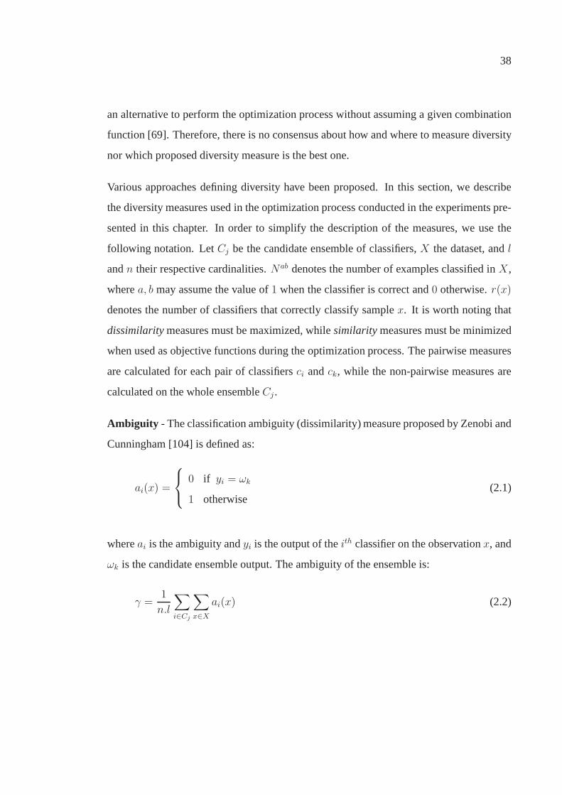
38

an alternative to perform the optimization process withoutassuming a given combination

function [69]. Therefore, there is no consensus about how and where to measure diversity

nor which proposed diversity measure is the best one.

Various approaches defining diversity have been proposed. In this section, we describe

the diversity measures used in the optimization process conducted in the experiments pre-

sented in this chapter. In order to simplify the descriptionof the measures, we use the

following notation. LetCj be the candidate ensemble of classifiers,X the dataset, andl

andn their respective cardinalities.Nab denotes the number of examples classified inX,

wherea, b may assume the value of1 when the classifier is correct and0 otherwise.r(x)

denotes the number of classifiers that correctly classify samplex. It is worth noting that

dissimilaritymeasures must be maximized, whilesimilarity measures must be minimized

when used as objective functions during the optimization process. The pairwise measures

are calculated for each pair of classifiersci andck, while the non-pairwise measures are

calculated on the whole ensembleCj .

Ambiguity - The classification ambiguity (dissimilarity) measure proposed by Zenobi and

Cunningham [104] is defined as:

ai(x) =

0 if yi = ωk

1 otherwise(2.1)

whereai is the ambiguity andyi is the output of theith classifier on the observationx, and

ωk is the candidate ensemble output. The ambiguity of the ensemble is:

γ =1

n.l

∑

i∈Cj

∑

x∈X

ai(x) (2.2)

39

Correlation Coefficient [44] - A pairwise similarity measure calculated as:

ρi,k =N11N00 −N01N10

√

(N11N10) + (N01N00) + (N11N00) + (N10N00)(2.3)

Difficulty Measure [44] - GivenF calculated from0l, 1l, . . . , 1, which represents the

number of classifiers inCj that correctly classify a patternx, this similarity measure may

be calculated as:

θ = V ar(F ) (2.4)

Disagreement[44] - A pairwise dissimilarity measure measured as:

ηi,k =N01 +N10

N11 +N10 +N01 +N00(2.5)

Double-fault [44] - A pairwise similarity measure defined as:

δi,k =N00

N11 +N10 +N01 +N00(2.6)

Entropy [44] - A dissimilarity measure which can be calculated as follows:

ξ =1

n

n∑

i=1

1

(l − ⌈l/2⌉)minr(xi), l − r(xi) (2.7)

Fault Majority - A pairwise dissimilarity measure proposed by Ruta and Gabrys [70]

which selects those classifiers with the highest probability of contributing to the majority

40

voting error of the classifier combination:

λ =

l∑

j=|l/2|

⌈l/2⌉∑

i∗=1

xi∗j (2.8)

xi∗j =

∑nk=1 .[1 − yi,k|m(xk) = 0]/n if j=0

l.∑n

k=1 .[1 − yi,k|m(xk) = 0]/nj otherwise(2.9)

wherem(xi) is the number of classifiers making error on observationxi, m(xi) = l −∑l

j=1 yi,j, and whereyi,j is 1 if correct and 0 otherwise, by classifierj and examplei.

Generalized Diversity [44] - A measure also based on the distributionY defined for the

coincident failure diversity. Lettingp(i), p(1), p(2) be the probability thati, 1 and 2

classifier(s) respectively, fail when classifying a samplex, we calculate:

p(1) =

l∑

i=1

i

lpi (2.10)

p(2) =

l∑

i=1

i

l

(i− 1)

(l − 1)pi (2.11)

The dissimilarity generalized diversity is calculated as:

τ = 1 −p(2)

p(1)(2.12)

Coincident Failure Diversity [44] - The result of a modification to Generalized Diver-

sity (Equation 2.12), which is based on the same distribution proposed for the difficulty

41

measure. Here, however,Y = il

denotes the proportion of classifiers that do not cor-

rectly classify a randomly chosen samplex. Therefore,Y = 1 − F (F from the difficulty

measure). It is also a dissimilarity measure, which is defined as follows:

σ =

0 p0 = 1.0

1(1−p0)

∑lq=1

ql

(q−1)(l−1)

pq p0 < 0(2.13)

Interrater Agreement [44] - A similarity measure written as:

κ = 1 −1l

∑ni=1 r(xi)(l − r(xi))

n(l − 1)p(1 − p)(2.14)

wherep is the average individual accuracy:

p =1

n.l

n∑

i=1

r(xi) (2.15)

Kohavi-Wolpert [44] - A dissimilarity measure calculated as:

ψ =1

n.l2

n∑

i=1

r(xi)(l − r(xi)) (2.16)

Q-Statics [44] - A pairwise measure calculated as:

Φi,k =N11N00 −N01N10

N11N00 +N01N10(2.17)

Summarizing, fourteen search criteria are used to guide theoptimization process of the

selection phase presented in this chapter. As shown in TableIII, these search criteria com-

prise twelve diversity measures, plus the ensemble’s combined error rate and ensemble

size.

42

Table III

List of search criteria used in the optimization process of the SOCS conducted in thischapter. The type specifies whether the search criterion must be minimized (similarity) or

maximized (dissimilarity)

Name Label TypeError rate ǫ SimilarityEnsemble size ζ SimilarityAmbiguity γ [104] DissimilarityCoincident failure diversity σ [44] DissimilarityCorrelation coefficient ρ [44] SimilarityDifficulty measure θ [44] SimilarityDisagreement η [44] DissimilarityDouble-fault δ [44] SimilarityEntropy ξ [44] DissimilarityFault majority λ [70] DissimilarityGeneralized diversity τ [44] DissimilarityInterrater agreement κ [44] SimilarityKohavi-Wolpert ψ [44] DissimilarityQ-statistic Φ [44] Similarity

2.2.2 Search Algorithms: Single- and Multi-Objective GAs

Single- andmulti-objectiveGA (MOGA) are the two strategies available when dealing

with GAs. Traditionally, when the optimization process is conducted as a single-objective

problem, GA is guided by an objective function during a fixed maximum number of gen-

erations (user definedmax(g)). The selection of classifier ensembles is applied in the

context of GA based on binary vectors. Each individual, called chromosome, is repre-

sented by a binary vector with a sizen, since the initial pool of classifiers is composed

of n members. Initially, a population with a fixed number of chromosomes is randomly

created, i.e. a random population of candidate classifier ensembles. Thus, at each genera-

tion stepg, the algorithm calculates fitness of each candidate ensemble in the population

C(g), which is the population of ensembles found at each generationg. The population is

evolved through the operators of crossover and mutation.

43

Figure 6(a) depicts an example of the evolution of the optimization process formax(g) =

1, 000 using GA as the search algorithm and the minimization of the error rateǫ as the

objective function. Even though we employedǫ as objective function, we show in Figure

6(a) plots ofǫ versus number of classifiersζ to better illustrate the problem. Each point on

the plot corresponds to a candidate ensembleCj taken fromP(C) and evaluated during the

optimization process. Indeed, these points represent the complete search space explored

for max(g) = 1, 000. The number of individuals at anyC(g) is 128. It is important to

mention that these candidate ensembles are projected onto the validation dataset in Figure

6(a), since our selection phase is conducted with validation. In SOCS, the solution with

lowest ǫ is selected as the best solutionC∗′j , which is further used to classify the test

samples, as shown in Figure 5. Diamond representsC∗′j in Figure 6(a).

10 20 30 40 50 60 70 80 90 100

4

6

8

10

12

14

Ensemble size

Err

or r

ate

Ensembles evaluated Cj

Best solution Cj*’

(a) GA guided byǫ

10 20 30 40 50 60 70 80 90 100

4

6

8

10

12

14

Ensemble size

Err

or r

ate

Ensembles evaluated C

j

Pareto front

Best solution Cj*’

(b) NSGA-II guided byǫ andζ

Figure 6 Optimization using GA with the error rateǫ as the objective function inFigure 6(a). Optimization using NSGA-II and the pair of objective functions:ǫ and ensemble sizeζ in Figure 6(b). The complete search space, the Paretofront (circles) and the best solutionC∗′

j (diamonds) are projected onto thevalidation dataset. The best performing solutions are highlighted by arrows.

MOGAs often constitute solutions to optimization processes guided by multi-objective

functions. Since the combination ofǫ and diversity measures as search criteria has been in-

vestigated in the literature as a strategy to select accurate and diverse candidate ensembles

44

[89; 104], MOGAs allow the simultaneous use of both measuresto guide the optimization

process of SOCS. These algorithms use Pareto dominance to reproduce the individuals.

A Pareto front is a set of nondominated solutions representing different tradeoffs between

the multi-objective functions. In our classifier ensemble selection application, a candi-

date ensemble solutionCi is said to dominate solutionCj , denotedCi Cj, if Ci is no

worse thanCj on all the objective functions andCi is better thanCj in at least one objec-

tive function. Based on this non-domination criterion, solutions over the Pareto front are

considered to be equally important.

Among several Pareto-based evolutionary algorithms proposed in the literature, NSGA-II

(elitist non-dominated sorting genetic algorithm) [11] appears to be interesting because

it has two important characteristics: a full elite-preservation strategy and a diversity-

preserving mechanism using the crowding distance as the distance measure. The crowding

distance does not need any parameter to be set [11]. Elitism is used to provide the means to

keep good solutions among generations, and the diversity-preserving mechanism is used

to allow a better spread among the solutions over the Pareto front. In addition, in appendix

1 we investigated three different MOGAs: (1) NSGA [11]; (2) NSGA-II [13]; and (3)

controlled elitist NSGA [14]. Our results indicated that the three MOGAs investigated

presented equivalent performances when guiding the optimization process.

NSGA-II [11] works as follows. At each generation stepg, a parent populationC(g) of

sizew evolves and an offspring populationCq(g), also of sizew, is created. These two

populations are combined to create a third populationCr(g) of size2w. The population

Cr(g) is sorted according to the nondominance criteria, and different nondominated fronts

are obtained. Then, the new populationC(g + 1) is filled by the fronts according to the

Pareto ranking. In this way, the worst fronts are discarded,since the size ofC(g + 1) is

w. When the last front allowed to be included inC(g + 1) has more solutions than the

C(g + 1) available free space, the crowding distance is measured in order to select the

45

most isolated solutions in the objective space in order to increase diversity. Algorithm 1

summarizes NSGA-II.

Algorithm 1 NSGA-II1: Creates initial populationC(1) of w chromosomes2: while g < max(g) do3: createsCq(g)4: setCr(g) = C(g) ∪C

q(g)5: perform a nondominated sorting toCr(g) and identify different frontsCk, k =

1, 2, . . . , etc6: while |C(g + 1)| + |Ck| ≤ w do7: setC(g + 1):=C(g + 1) ∪ Ck

8: setk:=k + 19: end while

10: perform crowding distance sort toCk

11: setC(g + 1):=C(g + 1) ∪ Ck⌊1 : (w − |C(g + 1)|)⌋12: createsCq(g + 1) from C(g + 1)13: setg:=g + 114: end while

The optimization process performed by NSGA-II formax(g) = 1, 000 is illustrated in

Figure 6(b). NSGA-II was employed, using the pair of objective functions: jointly mini-

mize the error rateǫ and the ensemble sizeζ . Circles on the plot represent the Pareto front.

Due to the fact that all solutions over the Pareto front are equally important, the selection

of the best candidate ensembleC∗′j is more complex. Several works reported in the liter-

ature take into account only one objective function to perform the selection. In [89], [51]

and [62], the candidate ensemble with lowestǫ was chosen as the best solutionC∗′j , even

though the optimization process was guided regarding multi-objective functions. We also

select the solution with lowestǫ asC∗′j , to classify the test samples in order to perform

SOCS in this chapter. Diamond indicates the solutionC∗′

j in Figure 6(b). In chapter 5 we

propose a dynamics SOCS to select the best candidate ensemble dynamically.

46

2.3 Experiments

A series of experiments has been carried out to investigate the search criteria and the search

algorithm we proposed to deal with at the beginning of this chapter. Our experiments are

broken down into three main series. In the first series, 13 different objective functions,

including the 12 diversity measures, are applied individually as single-objective functions.

In the second series, the diversity measures are used in pairs of objective functions com-

bined with the error rate in a multi-objective approach. Finally, the third series is per-

formed by applying pairs of objective functions combining either the diversity measures

or the error rate with ensemble size. We begin our analysis taking into account perfor-

mance (section 2.3.2), followed by a ensemble size analysis(section 2.3.3). It is important

to mention that all the experiments were replicated 30 timesand the results were tested

on multiple comparisons using the Kruskal-Wallis nonparametric statistical test by testing

the equality between mean values. The confidence level was 95% (α = 0.05), and the

Dunn-Sidak correction was applied to the critical values. First, we present a description

of the parameters settings on experiments.

2.3.1 Parameter Settings on Experiments

The details of the parameters used in our experiments are described here. These details

are related to the database, the ensemble construction method and the search algorithms.

Database

The experiments were carried out using the NIST Special Database 19 (NIST SD19)

which is a popular database used to investigate digit recognition algorithms. It is com-

posed of10 digit classes extracted from eight handwritten sample form(hsf) series, hsf-

0,1,2,3,4,6,7,8. It was originally divided into 3 sets: hsf-0123, hsf-7 and hsf-4. The

last two sets are referred here as data-test1 (60,089 samples) and data-test2 (58,646 sam-

ples). Data-test2 is well known to be more difficult to use forclassification than data-test1

47

[25]. On the basis of the results available in the literature, the representation proposed by

Oliveira et al. [52] appears to be well defined and well suitedto the NIST SD19 database.

The features are a combination of the concavity, contour andsurface of characters. The

final feature vector is composed of 132 components: 78 for concavity, 48 for contour and

6 for surface.

Ensemble Construction Method

As mentioned in section 2.1, RSS is used during the overproduction phase to generate an

initial pool of 100 kNN classifiers. Majority voting was usedas the combination func-

tion. This combination function is shown in Equation 1.1, chapter 1. In [89], rigorous

experimental tests were conducted to set up parameters suchas: k value and the number

of prototypes (to kNN classifiers), the number of subspace dimensions and the number of

classifier members to RSS, the size of the optimization and the size of the validation data

sets. The best parameters defined in [89] are used in this chapter. Table IV summarizes

the parameter sets used.

Table IV

Experiments parameters related to the classifiers, ensemble generation method anddatabase.

Number of nearest neighbors (k) 1Random subspace (number of features)32Training data set (hsf-0123) 5,000Optimization data set size (hsf-0123)10,000Validation data set (hsf-0123) 10,000Data-test1 (hsf-7) 60,089Data-test2 (hsf-4) 58,646

48

Genetic Algorithms

The population-based evolutionary algorithms used in thiswork are both single- and multi-

objective GAs. Since we use an initial pool composed of 100 classifiers, each individual is

represented by a binary vector with a size of 100. Experiments were carried out to define

the genetic parameters in [4]. Table V shows the parameter settings employed. The same

parameters were used for both GAs.

Table V

Genetic Algorithms parameters

Population size 128Number of generations 1000Probability of crossover 0.8Probability of mutation 0.01One-point crossover and bit-flip mutation

2.3.2 Performance Analysis

In order to define the best objective function for our problem, we carried out an experi-

mental investigation focusing on performance (recognition rate). The first question to be

answered is: Which measure is the best objective function for finding high-performance

classifier ensembles? Among the measures featured in section 2.2.1, the error rateǫ

(1−recognition rate) and the diversity measures are the most obvious candidates. The way

to compare these measures directly is to apply a single-objective optimization approach.

This direct comparison allows us to verify the possibility of using diversity insteadǫ to

find high-performance classifier ensembles.

Experiments with GA

GA-based experiments were conducted to compare 13 different objectives functions:ǫ

and the 12 diversity measures. As explained previously, each experiment was replicated

49

30 times in order to arrive at a better comparison of the results. Hence, each of the 13

objective functions employed generated 30 optimized classifier ensembles. Figure 7 shows

the comparison results of the 30 replications on data-test1(Figure 7(a)) and on data-test2

(Figure 7(b)).

ε γ σ ρ θ η δ ξ λ τ κ ψ Φ

3.5

4.0

4.5

5.0

5.5

6.0

6.5

7.0

Err

or r

ate

Objective Function

(a) data-test1

ε γ σ ρ θ η δ ξ λ τ κ ψ Φ

8.0

9.0

10

11

12

13

Err

or r

ate

Objective Function

(b) data-test2

Figure 7 Results of 30 replications using GA and 13 differentobjective functions. Theperformances were calculated on the data-test1 (Figure 7(a)) and on the data-test2 (Figure 7(b)).

These experiments show that:

a. Diversity measures are not better than the error rateǫ as an objective function for

generating high-performance classifier ensembles. The Kruskal-Wallis nonparamet-

ric statistical test shows thatǫ found ensembles which are significantly different

from those found by all the diversity measures.

b. The most successful diversity measure was the difficulty measureθ. However, the

performance of the classifier ensembles found using this measure was, on average,

0.12% (data-test1) and 0.31% (data-test2) worse than that of the ensembles found

usingǫ directly.

50

c. Fault majorityλ was the worst objective function. This is a different resultfrom

those presented by Ruta and Gabrys [70]. They observed that measures with better

correlation with majority voting error, i.e. fault majority and double-faultδ, are bet-

ter objective functions for generating high-performance ensembles than the others.

We found thatδ was the third best diversity measure andλ was the worst objective

function, even though there is no significant difference, according to the Kruskal-

Wallis statistical test, betweenλ, coincident failure, disagreement and entropy on

data-test1, and among the three first measures on data-test2.

The results achieved using GA were expected, apart from those for λ andδ. In fact, we

confirmed the results of previous work, e.g. [70] and [44], that diversity alone cannot

substitute forǫ as an objective function for finding the highest performing classifier en-

sembles. Since diversity alone is no better thanǫ, can we find better performing ensembles

by including both objective functions in the optimization process? We try to answer this

question using a multi-objective optimization approach inthe next section.

Experiments with NSGA-II

We continue our experimental study using NSGA-II as the search algorithm. The pre-

liminary study with GA suggested that diversity alone is notbetter thanǫ for generating

the best performing classifier ensemble. This observation led us to use bothǫ and diver-

sity jointly to guide the optimization process with NSGA-II, since we have the option of

combining different objective functions. The hope is that greater diversity between base

classifiers leads to the selection of high-performance classifier ensembles.

Each diversity measure mentioned in section 2.2.1 was combined withǫ to make up pairs

of objective functions to guide the optimization process. Again, the optimization process

using each pair of objective functions was replicated 30 times. Figure 8 shows the results

of 30 replications on data-test1 (Figure 8(a)) and data-test2 (Figure 8(b)). It is important

to mention that the first value corresponds to the results using GA as the search algorithm

51

ε ζ γ σ ρ θ η δ ξ λ τ κ ψ Φ3.40

3.45

3.50

3.55

3.60

3.65

3.70

3.75

3.80

3.85

Err

or r

ate

Objective Function

(a) data-test1

ε ζ γ σ ρ θ η δ ξ λ τ κ ψ Φ

7.4

7.5

7.6

7.7

7.8

7.9

8.0

8.1

8.2

8.3

Err

or r

ate

Objective Function

(b) data-test2

Figure 8 Results of 30 replications using NSGA-II and 13 different pairs of objectivefunctions. The performances were calculated on data-test1(Figure 8(a)) anddata-test2 (Figure 8(b)). The first value corresponds to GA with the error rateǫ as the objective function while the second value corresponds to NSGA-IIguided byǫ with ensemble sizeζ .

andǫ as the objective function. This means that we can compare thesingle- and multi-

objective results. The second value corresponds to the results using NSGA-II guided by

ensemble sizeζ , with ǫ as the objective functions (discussed in the next section).

Some observations can be made from these results:

a. By including both diversity andǫ in a multi-objective optimization process, we may

find more high-performance classifier ensembles than by using diversity alone; how-

ever, the performance of these ensembles is still worse thanthe performance of the

ensembles found usingǫ in the single-objective optimization process.

b. The best diversity measures are difficultyθ, interrater agreementκ, correlation co-

efficientρ and double-faultδ on data-test1. The Kruskal-Wallis test shows that the

first three measures found classifier ensembles with no significantly different mean

ranks from those found using GA withǫ as the objective function on data-test1. On

52

data-test2, almost all the diversity measure results were similar. According to the

Kruskal-Wallis statistical test, except for coincident failure σ andθ, all the diversity

measures found classifier ensembles with no significantly different mean ranks on

data-test2. It is important to note that the difference between ensembles found using

diversity (multi-objective optimization) and ensembles found using onlyǫ (single-

objective optimization) was dramatically less. The classifier ensembles found using

the three best diversity measures were, on average, 0.05% worse than those found

using onlyǫ on data-test1 and 0.13% worse on data-test2.

c. It is interesting to note thatθ found high-performance classifier ensembles on data-

test1, but, on data-test2,θ yielded one of the worst performances. Such behavior

shows that these two data sets are actually very different.

d. The two measures pointed out by Ruta and Gabrys [70] as the best diversity mea-

sures (δ andλ) found better classifier ensembles on multi-objective thanon single-

objective optimization, as was the case for all the measures. However, especially

on data-test1,λ was the worst measure, and, once again, was significantly different

from the other measures, as shown by the Kruskal-Wallis test.

As indicated in the beginning of this chapter, besides performance, we have to take into

account ensemble size when selecting classifier ensembles.In the following section, this

aspect is analyzed.

2.3.3 Ensemble Size Analysis

Our ensemble size analysis relies on the analogy between feature subset selection and

SOCS. In this sense, discarding redundant classifiers couldimprove performance. Hence,

the minimization of the ensemble sizeζ is the most obvious objective function to use to

achieve such a reduction in the number of classifiers. However, ζ cannot be used in a

single-objective optimization process, because it might be combined with other measures

53

in order to increase performance while reducing the number of classifiers. In line with

this idea, we combineζ with ǫ and the 12 diversity measures described in section 2.2.1

to make up pairs of objective functions to guide the optimization process using NSGA-

II. Figure 9 presents a graph containing the size of the classifier ensembles found in 30

replications generated by each pair of objective functions, while the performances are

shown in Figure 10 (10(a), data-test1 and 10(b), data-test2). The first value corresponds

to the results obtained using GA as the search algorithm andǫ as the objective function in

order to arrive at a better comparison.

ε ζ γ σ ρ θ η δ ξ λ τ κ ψ Φ

5

10

15

20

25

30

35

40

45

50

Ens

embl

e si

ze

Objective Function

Figure 9 Size of the classifier ensembles found using 13 different measures combinedwith ensemble sizeζ in pairs of objective functions used by NSGA-II.

We also show the ensemble size of the classifier ensembles found in the first two series

of experiments, i.e., single objective functions and diversity combined withǫ. This allows

us to better analyze the ensemble size issue. Figure 11 showsthe ensemble size of the

classifier ensembles found with GA (Figure 11(a)) and with NSGA-II combining ǫ with

diversity (Figure 11(b)). Based on all these results, we observe that:

a. Diversity combined withζ in pairs of objective functions does not find high-

performance classifier ensembles. Taking into account all the results obtained in all

the series of experiments, the performances of the ensembles found using these pairs

54

ε ζ γ σ ρ θ η δ ξ λ τ κ ψ Φ

3.5

4.0

4.5

5.0

5.5

6.0

6.5

Err

or r

ate

Objective Function

(a) data-test1

ε ζ γ σ ρ θ η δ ξ λ τ κ ψ Φ

7.5

8.0

8.5

9.0

9.5

Err

or r

ate

Objective Function

(b) data-test2

Figure 10 Performance of the classifier ensembles found using NSGA-II with pairs ofobjective functions made up of ensemble sizeζ and the 13 different measures.Performances were calculated on data-test1 (Figure 10(a))and on data-test2(Figure 10(b)).

ε γ σ ρ θ η δ ξ λ τ κ ψ Φ0

10

20

30

40

50

60

Ens

embl

e si

ze

Objective Function

(a) GA

ε ζ γ σ ρ θ η δ ξ λ τ κ ψ Φ0

10

20

30

40

50

60

Ens

embl

e si

ze

Objective Function

(b) NSGA-II

Figure 11 Ensemble size of the classifier ensembles found using GA (Figure 11(a)) andNSGA-II (Figure 11(b)). Each optimization process was performed 30 times.

of objective functions made up ofζ and diversity showed the worst performances.

In contrast, those ensembles were the smallest. It is interesting to note that, using

this combination of objective functions, NSGA-II converges to the same solution

55

at each replication, with the exception of the difficulty measureθ. The minimum

number of classifiers allowed by the search algorithms was 5.This fixed minimum

ensemble size was defined to avoid generating too small classifier ensembles.

b. The most successful diversity measure in terms of performance wasθ. However, the

performance of the ensembles obtained usingζ andǫ are better. According to the

Kruskal-Wallis statistical test, the performances are significantly different.

c. The analogy between FSS and SOCS may be established. The performance of our

baseline system, i.e. the pool of 100 kNN (96.28% on data-test1), is 0.07% worse

than the average result usingζ andǫ as the objective functions (average of 96.35%

on data-test1 (Figure 10), while the averaged ensemble sizeis 27 classifiers (Figure

40). However, better performing classifier ensembles can befound using GA and

ǫ. The Kruskal-Wallis statistical test showed that the performances are significantly

different. Moreover, the combination ofζ andǫ as the objective function did not

establish the best trade-off between these two measures. Interrater agreementκ

combined withǫ generated smaller (24 classifiers on average) and better performing

classifier ensembles (96.41% and 92.16%, on average, on data-test1 and on data-

test2 respectively, Figure 8).

d. Ambiguityγ combined withǫ, and Kohavi-Wolpertψ combined withǫ, found the

largest classifier ensembles (45 classifiers on average). What is more interesting is

that, although we found the best performing classifier ensemble using GA as the

search algorithm andǫ as the objective function, such single-objective functiondid

not find the largest solutions.

2.4 Discussion

This chapter presented the experimental results of a study using the single- and multi-

objective optimization processes to perform the selectionphase of SOCS. An ensemble

56

of 100 kNN classifiers generated using the Random Subspace method was used as the

initial pool of classifiers. Fourteen different objective functions were applied: 12 diversity

measures, error rate and ensemble size. The experiments were divided into three series. In

the first, the error rate and the 12 diversity measures were directly compared in a single-

optimization approach. In the second, the 12 diversity measures were combined with the

error rate to make up pairs of objective functions in a multi-optimization approach. Finally,

in the third, the error rate and the 12 diversity measures were combined with ensemble size

in pairs of objective functions, again in a multi-optimization approach.

The first series of experiments was conducted in order to answer the first question (1)

posed in the beginning of this chapter. Our results confirm the observation made in pre-

vious work that diversity alone cannot be better than the error rate at finding the most

accurate classifier ensembles. The difficulty measure was the best diversity measure when

the diversity measures are compared. In our attempt to answer question (2) when both the

error rate and diversity are combined in a multi-objective approach (second series of ex-

periments), we found that the performance of the solutions using diversity is much higher

than the performance of the solutions using diversity in a single-objective optimization

approach. However, the performance of the classifier ensembles found using diversity

measures combined with the error rate to guide the selectionwere still worse than the per-

formance of the ensembles found using only the error rate, although the difference was

reduced.

We are now able to establish an analogy between feature subset selection and SOCS, in

response to question (3). By combining ensemble size and theerror rate in a pair of ob-

jective functions, we increased the initial pool of classifier performances and decreased

the number of classifiers to 27, instead of 100, from the initial pool. In contrast, diversity

measures achieved the worst performance in the third seriesof experiments. Moreover,

the combined minimization of ensemble size and error rate was not the best pair of objec-

tive functions to accomplish the trade-off between complexity and performance. In fact,

57

interrater agreement combined with the error rate established the best trade-off between

performance and ensemble size. We conclude, therefore, that it is not necessary to include

ensemble size in the optimization process. The reduction inthe number of classifiers is a

consequence of the selection of classifiers, whatever the objective function used to guide

the search. Some objective functions generate smaller classifier ensembles, while others

generate bigger ones.

It is also important to observe that our experiments showed that ensemble size and di-

versity are not conflicting objective functions (see Figure9). We observe that we cannot

decrease the generalization error rate by combining this pair of objective functions. In

appendix 3, we present further evidence to show why diversity and ensemble size are not

conflicting objective functions. Moreover, we can see in Table XXIV and Table XXV in

appendix 2, that the results obtained using diversity measures in a single-objective opti-

mization approach are quite similar to the results obtainedusing diversity combined with

ensemble size in pairs of objective functions in a multi-objective optimization approach.

Hence, the minimum number of classifiers is achieved when using most of the diversity

measures in single-objective optimization (see Figure 11(a)). Thus, the results related to

the first series of our experiments may be different if the minimum number of classifiers

is fixed and larger than we have defined in this chapter, i.e. 5 classifiers.

Moreover, in this chapter, we conducted the optimization processes using, besides the

traditional optimization dataset, a validation dataset inorder to avoid overfitting during

the selection phase of SOCS. Despite such apparent overfitting control, we observed that

this strategy fails to address the overfitting phenomenon since, although an independent

dataset was used to validate the solutions, the overfitting phenomenon may still be present.

In the next chapter we show that overfitting can be detected atthe selection phase of SOCS

and present strategies to control overfitting.

CHAPTER 3

OVERFITTING-CAUTIOUS SELECTION OF CLASSIFIER ENSEMBLES

We show in this chapter that overfitting can be detected during the selection phase of

SOCS, this selection phase being formulated as an optimization problem. We attempt to

prove experimentally that an overfitting control strategy must be conductedduring the

optimization process. In order to pursue our analysis on population-based evolutionary

algorithms, we keep using both single- and multi-objectiveGA. Taking into account this,

we investigate the use of an auxiliary archiveA to store the best performing candidate

ensembles (or Pareto fronts in the MOGA case) obtained in a validation process using the

validation partitionV to control overfitting. Three different strategies for updateA have

been compared and adapted in this chapter to the context of the single- and multi-objective

selection of classifier ensembles: (1)partial validationwhereA is updated only in the last

generation of the optimization process; (2)backwarding[67] which relies on monitoring

the optimization process by updatingA with the best solution from each generation; and

(3) global validation[62] updatingA by storing in it the Pareto front (or the best solution

in the GA case) identified onV at each generation step.

Besides the ensemble of kNN created at the overproduction phase using the RSS method

in the previous chapter, two additional initial pool of classifiers are investigated in this

chapter: (1) a pool of DT created using bagging; and (2) a poolof DT created using the

RSS method. In addition, considering the results related tothe analysis of search criteria

obtained previously, we use only four diversity measures (described in section 2.2.1) andǫ

to guide the optimization process presented in this chapter. Diversity measures are applied

by NSGA-II in combination withǫ in pairs of objective functions. Moreover,ǫ, as well

as the diversity measures, are employed as single-objective functions by GA. To avoid

the problem of reaching a too small ensemble size, we defined alarge fixed minimum

ensemble size for all diversity measures in our experiments. It is important to mention

59

that in appendix 2, we carried out an overfitting analysis using both GA and NSGA-II,

guided by all the objective functions and combinations of objective functions discussed

previously.

In this chapter, the global validation strategy is presented as a tool to show the relationship

between diversity and performance, specifically when diversity measures are used to guide

GA. The assumption is that, if a strong relationship exists between diversity and perfor-

mance, the solution obtained by performing global validation solely guided by diversity

should be close, or equal, to the solution with the highest performance among all solutions

evaluated. This offers a new possibility for analyzing the relationship between diversity

and performance, which has received a great deal of attention in the literature [44; 17; 70].

Our objective in this chapter is to answer the following questions:

1. Which is the best strategy employing an archiveA for reducing overfitting at the

selection phase of SOCS when this selection is formulated asan optimization prob-

lem?

2. Are classifier ensembles generated by bagging and RSS equally affected by overfit-

ting in the selection of classifier ensembles?

The following section demonstrates the circumstances under which the process of classi-

fier ensemble selection results in overfitting. In section 3.2, three strategies used to control

overfitting are introduced. The parameters employed for theexperiments are described

in section 3.3, where the validation strategies are appliedusing holdout andk-fold cross-

validation schemes. Finally, experimental results are presented in section 3.3.

3.1 Overfitting in Selecting Classifier Ensembles

The problem of selecting classifier ensembles, using an optimization datasetO can be for-

mulated as a learning task, since the search algorithm operates by minimizing/maximizing

60

the objective function, such as maximizing the classification performance or maximizing

the diversity of the members of a given ensembleCj. Indeed, Radtke et al. [62] showed

that multi-objective evolutionary optimization, such as the selection of classifier ensem-

bles, is prone to overfitting. We may define overfitting in the context of ensemble selection

inspired by the definition provided by Mitchell [49] in the following way. LetC∗j andC∗′

j

be the best performing candidate ensembles found through calculating the error rateǫ for

each element ofP(C) over samples contained inO andV respectively. Consider the clas-

sification errorǫ of these two candidate ensembles measured using samples from V. We

will denote this classification error byǫ(V, C∗j ) andǫ(V, C∗′

j ). In this setting,C∗j is said

to overfit onO if an alternative candidate ensembleC∗′j ∈ P(C) can be found such that

ǫ(V, C∗j ) > ǫ(V, C∗′

j ).

The selection process for classifier ensembles in SOCS is illustrated in Figure 12. An en-

semble creation method is employed usingT to generate the initial pool of classifiersC.

Thus, the search algorithm calculates fitness onO by testing different candidate ensem-

bles. The best candidate ensembleC∗′j is identified inV to prevent overfitting. Finally, the

generalization performance ofC∗′j is measured using the test dataset (G). Hence, SOCS

requires at least these four datasets. It is important to mention thatV is different from

the validation dataset typically used to adjust base classifier parameters, such as weights

in MLP, the number of neighbors considered (k value) in kNN classifiers, etc. When

such parameter adjustment is necessary, a fifth dataset mustbe used, as was done in [62],

to avoid overly optimistic performance assessment. The following sections describe how

overfitting can be detected in single- and multi-objective optimization problems performed

by GAs.

3.1.1 Overfitting in single-objective GA

In Figure 13,ǫ is employed as the objective function to guide GA using the NIST-digits

database as the problem and RSS as the method to generateC as a pool of 100 kNN clas-

61

EnsembleGeneration

MethodProcess

# generations

ssentif

Optimization

G

C∗′j

O

C = c1, c2, . . . , cn

T

V

OV

C∗j

C∗′j fromA

xi,t xi,o

xi,v

ωk

OVERPRODUCTION PHASE SELECTION PHASE

xi,g

Figure 12 Overview of the process of selection of classifier ensembles and the points ofentry of the four datasets used.

sifiers. These same parameters were investigated in last chapter, section 2.3.1. Although

GA was only guided byǫ, we show plots ofǫ versus the ensemble’s size to better illustrate

the process.

We denoteC(g) as the population of candidate classifier ensembles found ateach genera-

tion g and the best candidate ensemble found by evaluating all individuals fromC(g) on

O by C∗j (g). Each point on the plot corresponds to a candidate ensembleCj taken from

P(C) and evaluated during the optimization process. Indeed, these points represent the

complete search space explored formax(g) = 1, 000. The number of individuals at any

C(g) is 128.

Actually, the overfitting phenomenon measured when selecting classifier ensembles

presents a behavior very similar to what is seen in a typical Machine Learning process,

i.e. the chance that the search algorithm will overfit on samples taken fromO increases

with the number of generations. This phenomenon can be observed in Figure 13(e), which

shows the evolution ofǫ(O, C∗′j ) in the search space. On the one hand, it is clear that the

optimization process could be stopped before overfitting starts to occur in this problem

62

20 30 40 50 60 70 80 90 1003.0

3.2

3.4

3.6

3.8

4.0

4.2

4.4

4.6

4.8

5.0

Ensemble size

Err

or r

ate

Cj (evaluated)

Cj*(1)

(a) O dataset andg = 1

20 30 40 50 60 70 80 90 1003.0

3.2

3.4

3.6

3.8

4.0

4.2

4.4

4.6

4.8

5.0

Ensemble size

Err

or r

ate

Cj (to evaluate)

Cj (evaluated)

Cj*(1)

(b) V dataset andg = 1

20 30 40 50 60 70 80 90 1003.0

3.2

3.4

3.6

3.8

4.0

4.2

4.4

4.6

4.8

5.0

Ensemble size

Err

or r

ate

Cj (to evaluate)

Cj (evaluated)

Cj*(52)

(c) O dataset andg = 52

20 30 40 50 60 70 80 90 1003.0

3.2

3.4

3.6

3.8

4.0

4.2

4.4

4.6

4.8

5.0

Ensemble size

Err

or r

ate

Cj (to evaluate)

Cj (evaluated)

Cj*(52)

(d) V dataset andg = 52

20 30 40 50 60 70 80 90 1003.0

3.2

3.4

3.6

3.8

4.0

4.2

4.4

4.6

4.8

5.0

Ensemble size

Err

or r

ate

Cj

Cj*

Cj*’

(e) O dataset andmax(g)

20 30 40 50 60 70 80 90 1003.0

3.2

3.4

3.6

3.8

4.0

4.2

4.4

4.6

4.8

5.0

Ensemble size

Err

or r

ate

Cj

Cj*

Cj*’

overfitting

(f) V dataset andmax(g)

Figure 13 Optimization using GA guided byǫ. Here, we follow the evolution ofC∗j (g)

(diamonds) fromg = 1 to max(g) (Figures 13(a), 13(c) and 13(e)) onthe optimization datasetO, as well as on the validation datasetV (Figures13(b), 13(d) and 13(f)). The overfitting is measured as the difference in errorbetweenC∗′

j (circles) andC∗j (13(f)). There is a 0.30% overfit in this example,

where the minimal error is reached slightly afterg = 52 onV, and overfittingis measured by comparing it to the minimal error reached onO. Solutions notyet evaluated are in grey and the best performing solutions are highlighted byarrows.

63

using GA. On the other, it is difficult to define a stopping criterion to control overfitting in

a multi-objective optimization process, as explained in section 3.1.2.

3.1.2 Overfitting in MOGA

Figure 14 (left) illustrates the optimization process performed formax(g) = 1, 000 using

NSGA-II guided by the following pair of objective functions: jointly minimize ǫ and dif-

ficulty measure (section 2.2.1) in the same problem investigated with GA in last section.

The Pareto front from populationC(g) found inO is denoted byCk(g). Thus,C∗k (dia-

monds) andC∗′

k (circles) represent the final Pareto fronts found inO andV respectively.

Especially noteworthy in Figure 14(f) is that, besides the fact that the solutions overC∗′

k

are different from solutions overC∗k, which was expected considering thatV andO are dif-

ferent datasets, the nondominated solutions overC∗′

k are discarded during the optimization

process (Figure 14(e)). Hence, the definition of a stopping criterion for multi-objective op-

timization problems is difficult for the following reasons:(1) solutions overCk(g) found

during the optimization process may not be nondominated solutions overV and (2) since

the evolution ofCk(g) must be monitored onV, comparing sets of equally important so-

lutions is a complex task. We show in the next section that theuse of an auxiliary archive

A makes it possible to control overfitting taking into accountthese aspects.

3.2 Overfitting Control Methods

The focus of this chapter is to evaluate strategies that relyon usingV to create an archive

A to control overfitting, since these memory-based strategies may be applied in any op-

timization problem. The idea is to use the error rate measured on V as an estimation

of the generalization error. In order to accomplish the objectives of this chapter, we have

adapted two overfitting control strategies to the context ofclassifier ensemble selection for

both single- and multi-objective optimization problems: (1) backwardingoriginally pro-

posed in [67] to prevent overfitting in GP; and (2)global validationproposed in [62] and

64

0.035 0.036 0.037 0.038 0.039 0.04 0.041 0.042 0.0433.0

3.2

3.4

3.6

3.8

4.0

4.2

4.4

4.6

4.8

5.0

Difficulty Measure

Err

or r

ate

Cj (to evaluate)

Cj (evaluated)

Ck(1)

(a) O dataset andg = 1

0.035 0.036 0.037 0.038 0.039 0.04 0.041 0.042 0.0433.0

3.2

3.4

3.6

3.8

4.0

4.2

4.4

4.6

4.8

5.0

Difficulty Measure

Err

or r

ate

Cj (to evaluate)

Cj (evaluated)

Ck(1)

(b) V dataset andg = 1

0.035 0.036 0.037 0.038 0.039 0.04 0.041 0.042 0.0433.0

3.2

3.4

3.6

3.8

4.0

4.2

4.4

4.6

4.8

5.0

Difficulty Measure

Err

or r

ate

Cj (to evaluate)

Cj (evaluated)

Ck(15)

(c) O dataset andg = 15

0.035 0.036 0.037 0.038 0.039 0.04 0.041 0.042 0.0433.0

3.2

3.4

3.6

3.8

4.0

4.2

4.4

4.6

4.8

5.0

Difficulty Measure

Err

or r

ate

Cj (to evaluate)

Cj (evaluated)

Ck(15)

(d) V dataset andg = 15

0.035 0.036 0.037 0.038 0.039 0.04 0.041 0.042 0.0433.0

3.2

3.4

3.6

3.8

4.0

4.2

4.4

4.6

4.8

5.0

Difficulty Measure

Err

or r

ate

Cj

Ck*

Ck*’

(e) O dataset andmax(g)

0.035 0.036 0.037 0.038 0.039 0.04 0.041 0.042 0.0433.0

3.2

3.4

3.6

3.8

4.0

4.2

4.4

4.6

4.8

5.0

Difficulty Measure

Err

or r

ate

Cj

Ck*

Ck*’

overfitting

(f) V dataset andmax(g)

Figure 14 Optimization using NSGA-II and the pair of objective functions: difficultymeasure andǫ. We follow the evolution ofCk(g) (diamonds) fromg = 1to max(g) (Figures 14(a), 14(c) and 14(e)) on the optimization dataset O,as well as on the validation datasetV (Figures 14(b), 14(d) and 14(f)). Theoverfitting is measured as the difference in error between the most accuratesolution inC

∗′

k (circles) and inC∗k (14(f)). There is a 0.20% overfit in this

example, where the minimal error is reached slightly afterg = 15 onV, andoverfitting is measured by comparing it to the minimal error reached onO.Solutions not yet evaluated are in grey.

65

[67] to control overfitting in multi-objective evolutionary optimization problems.Partial

validation, a control strategy traditionally used to avoid overfittingin classifier ensemble

selection problems [89] is also investigated. This is the strategy used in previous chapter.

It is interesting to note that these strategies can be ordered with respect to the cardinality

of the solution set used for overfitting control:partial validationuses only the last popu-

lation of solutions (orC∗k in the MOGA case) andbackwardingvalidates the best solution

(or C∗k(g)) at eachg, while global validationuses all solutions at eachg.

It is important to note that theglobal validationstrategy is employed in [62] in a complex

two-level system which includes feature extraction, feature selection and classifier ensem-

ble selection, all performed by MOGA. In this thesis, we adapt their strategy to single-

objective GA. As mentioned earlier, we use ensembles generated by bagging (BAG) and

RSS.

3.2.1 Partial Validation (PV)

The first and simplest procedure relies on selectingC∗′j at the end of the optimization

process by validating the last populationC(max(g)) (for GA) or C∗k (respectively for

MOGA). Consequently, in PV, it is assumed that,C∗′j ∈ C(max(g)) andC∗′

j ∈ C∗k.

Hence, there is only one update onA, more precisely formax(g). PV is summarized in

Algorithm 2.

Algorithm 2 Partial Validation1: Creates initial populationC(1) of w chromosomes2: A = ∅3: for each generationg ∈ 1, . . . , max(g) do4: perform all genetic operators and generate new populationC(g + 1).5: end for6: validate all solutions fromC(max(g)) (for GA) or C∗

k (for MOGA)7: choose asC∗′

j the solution with highest recognition rate8: updateA by storingC∗′

j

9: return C∗′j stored inA

66

3.2.2 Backwarding (BV)

Overfitting remains uncontrolled even when PV is used, becauseC(max(g)) (for GA)

or C∗k for MOGA are composed of overfitted solutions, as explained in section 3.1. An

alternative to PV is to validate not onlyC(max(g)) (or C∗k), but theC∗

j (g) (or Ck(g))

found at each generation. The BV method [67] proposed for GP problems is based on this

idea. The authors advocate that GP is prone to overfitting especially on later generations

as in Machine Learning tasks. Motivated by this observation, they proposed BV to control

overfitting by monitoring the optimization process onV to determine the point where GP

starts to overfitO. This approach usesA to store the best solution found before overfitting

starts to occur. Even thoughǫ is not the only objective function used to guide GA in this

chapter, we useǫ to represent the objective function in Algorithm 3, which shows how

BV is employed with GA. However, other objective functions can be used without loss of

generality.

Algorithm 3 Backwarding for GA1: Creates initial populationC(1) of w chromosomes2: A = ∅3: FindC∗

j (1) and setC∗′j := C∗

j (1)

4: StoreC∗′j in A

5: for each generationg ∈ 1, . . . , max(g) do6: perform all genetic operators7: generate new populationC(g + 1) and findC∗

j (g + 1) as usual8: if ǫ(V, C∗

j )(g + 1) < ǫ(V, C∗′

j ) then9: setC∗′

j := C∗j (g + 1)

10: updateA by storing in it the newC∗′j

11: end if12: end for13: return C∗′

j stored onA

Where multi-objective optimization is concerned, Pareto fronts must be stored inA instead

of individual solutions. Taking into account that BV relieson comparing each new solution

found onO to the solution stored onA, this fact leads to the following question: How can

67

Pareto fronts be compared so as to identify whether or not onePareto front is better than the

others. Because of the various tradeoffs over the Pareto front, the definition of a quality

measure is much more complex in multi-objective than in single-objective optimization

problems. Some quality measures such as the Pareto front spread, the objective functions

spread [103], the epsilon indicator and the coverage function [108] have been proposed. In

order to determine whether or not theCk(g) found at each generation is better than theC∗′

k

stored inA, we propose to use the Pareto quality measure called thecoveragefunction,

introduced by Zitzler et al. [108]. This measure was used in [61] to define a stopping

criterion for MOGAs.

The coverage function, measured onV, is based on the weak dominance criteria and indi-

cates the number of candidate ensembles inCk(g) that are weakly dominated by at least

one solution inC∗′

k . Given two solutionsCi ∈ C∗′

k andCj ∈ Ck(g), we may say thatCi

coversCj if Ci is not worse thanCj in all objective functions. The idea is to verify the

Pareto improvement among generations onA. Coverage can be denoted as:

cov(C∗′

k ,Ck(g)) (3.1)

In this way, the average number of solutions inC∗′

k covering the solutions onCk(g) is

calculated. Thus,cov(C∗′

k ,Ck(g)) < 1 or cov(C∗′

k ,Ck(g)) = 1, whetherC∗′

k covers the

entire ParetoCk(g) or not. The Pareto improvement at each generation is then measured

as:

imp(Ck(g),C∗′

k ) = 1 − cov(C∗′

k ,Ck(g)) (3.2)

Improvement reaches its maximum (imp = 1) when there is no solution onCk(g) cov-

ered by solutions onC∗′

k and its lowest possible value(imp = 0), when all solutions on

Ck(g) are covered by those onC∗′

k . Consequently, the update ofA is dependent on the

68

improvement obtained between these two Pareto fronts. Whenimp > 0, A is updated;

otherwise, there is no update. The BV for MOGA is summarized in Algorithm 4.

Algorithm 4 Backwarding for MOGA1: Creates initial populationC(1) of w chromosomes2: A = ∅3: FindCk(1) and setC∗′

k :=Ck(1)4: StoreC∗′

k in A5: for each generationg, g ∈ 1, . . . , max(g) do6: perform all genetic operators;7: generateC(g + 1) and findCk(g + 1) as usual8: if imp(Ck(g + 1),C∗′

k ) > 0 then9: setC∗′

k :=Ck(g + 1)10: updateA by storing in it the newC∗′

k

11: end if12: end for13: return C

∗′

k stored onA to pick upC∗′j .

3.2.3 Global Validation (GV)

There is a problem with BV because, since, at each generation, GA (or MOGA) creates

a population of solutions,C∗j (g) (or Ck(g) for MOGA) found onO may not be the best

solution (or Pareto front) onV. An approach avoiding such a limitation is global validation

GV [62; 100], which relies on usingA to validate the entire populationC(g) from each

generation.

GV works as follows in the context of multi-objective optimization (Algorithm 5): at each

g step, all solutions are validated, and thus the set of non-dominated solutions found onV

is stored inA. When the optimization process is completed, two sets of non-dominated

solutions are available: (1) the traditionalC∗k found onO; and (2)C∗′

k , the set of non-

dominated solutions found onV. In Figure 14(f), the solutions composingC∗′

k stored inA

are represented by circles. As can be observed in this figure,the solutions stored inA are

different from the solutions overC∗k.

69

Algorithm 5 Global Validation for MOGA1: Creates initial populationC(1) of w chromosomes2: A = ∅3: for each generationg ∈ 1, . . . , max(g) do4: perform all genetic operators5: generateC(g + 1)6: validate all solutions inC(g + 1) over samples contained inV7: perform a nondominated sorting toC(g + 1) ∪A to findC

∗′

k

8: updateA by storing in itC∗′

k

9: end for10: return C

∗′

k stored inA

We propose to change Radtke et al.’s method [62] slightly to adapt it to single-objective

optimization problems. Since no Pareto front is involved when using GA, we are interested

in the best solutionC∗′j . In this case, it is sufficient to validate all solutions at each new

generation, find the best solutionC∗′j (g) and compare it toC∗′

j , which is stored inA. In

this way, we keep the solutionC∗′

j found onV stored inA. Lettingǫ represent the objective

function, the complete GV algorithm for GA is described in Algorithm 6.

Algorithm 6 Global Validation for GA1: Creates initial populationC(1) of w chromosomes2: A = ∅3: Validate all solutions inC(1) over samples contained inV4: FindC∗′

j (1) from C(1)

5: SetC∗′j :=C∗′

j (1)6: for each generationg ∈ 1, . . . , max(g) do7: perform all genetic operations and generateC(g + 1)8: validate all solutions inC(g + 1)9: findC∗′

j (g + 1)

10: if ǫ(V, C∗′j )(g + 1) < ǫ(V, C∗′

j ) then11: setC∗′

j := C∗′j (g + 1)

12: updateA by storing in it the newC∗′j

13: end if14: end for15: return C∗′

j stored inA

An example of the GV strategy for single-objective GA is illustrated in Figure 13(f). This

figure shows overfitting when comparingǫ(V, C∗′j ) andǫ(V, C∗

j ). The ensembleC∗′j prob-

70

ably has higher generalization performance thanC∗j obtained inO. In section 3.3, we

analyze such an assumption experimentally.

3.3 Experiments

The parameters and the experimental protocol employed are described in sections 3.3.1

and 3.3.2 respectively.

3.3.1 Parameter Settings on Experiments

The databases, ensemble construction methods, search algorithms and objective functions

used to conduct the experiments are defined in this section.

Databases

It is important to note that the databases must be large enough to be partitioned into the four

above-mentioned datasets:T , O, V andG, to perform experiments using the holdout val-

idation strategy, as was done in the previous chapter. However, very few large databases

containing real classification problems are available in the literature. SOCS is general

enough to be conducted using small datasets by applyingk-fold cross-validation. Ac-

cordingly, we performed experiments using both the holdoutand 10-fold cross-validation

strategies. Another important aspect taken into account inselecting the databases for our

experiments is that relatively high-dimensional feature spaces are necessary for the RSS

method.

Two databases were used in the holdout validation experiments: (1) NIST Special

Database 19 containing digits (NIST SD19), used in the previous chapter, which we call

NIST-digits here; and (2) NIST SD19 containing handwrittenuppercase letters, which we

call NIST-letters here. We use the representation proposedby Oliveira et al. [52] for

both databases. Table VI lists important information aboutthese two databases and the

partitions used to compose the four separate datasets. These same partitions were used

71

in [89] for NIST-digits and in [61] for NIST-letters. We usedthe two test datasets from

NIST-digits, as was done in the previous chapter.

Table VI

Specifications of the large datasets used in the experimentsin section 3.3.3.

Dataset # of Training Optimization Validation Test Features PoolCfeatures Set (T ) Set (O) Set (V) Set (G) RSS size

NIST-digits 132 5,000 10,000 10,000 test1 60,089 32 100test2 58,646

NIST-letters 132 43,160 3,980 7,960 12,092 32 100

Table VII describes the three databases used in the 10-fold cross-validation experiments:

dna, texture and satimage. TheDna andsatimagedatasets are provided by Project Statlog

on www.niaad.liacc.up.pt/old/statlog; andtexture is available within the UCI machine

Learning Repository.

Table VII

Specifications of the small datasets used in the experimentsin section 3.3.4.

Dataset # of samples # of features Features RSS PoolC sizedna 3186 180 45 100texture 5500 40 20 100satimage 6435 36 18 100

Ensemble Construction Methods and Base Classifiers

We chose kNN and DT as the base classifiers in our experiments.The C4.5 algorithm [60]

(Release 8) was used to construct the trees with pruning. In addition, we usedk = 1 for

kNN classifiers in all databases without fine-tuning this parameter in order to avoid addi-

tional experiments. BAG and RSS were applied to generate theinitial pools of classifiers

in our experiments. Three initial pools of 100 classifiers were created: (1) 100 DT and (2)

72

100 kNN, which were generated using RSS, and (3) 100 DT, whichwas generated using

BAG (BAG is mostly effective with unstable classifiers, suchas DT). The size of the sub-

sets of features used by RSS is shown in Table VI for large datasets and in Table VII for

small datasets. The same subspaces are used for both kNN and DT classifiers. Majority

voting was used as the combination function.

Objective Functions

In order to reduce redundancy in our experiments, we chose toemploy only four diversity

measures: (1) difficulty measure (θ), which was pointed out as the best diversity measure

when the diversity measures were compared in single-objective optimization problems; (2)

double-fault (δ), which was one of the best diversity measure used in combination with the

error rate to guide NSGA-II, (3) coincident failure diversity (σ), which was chosen due to

the conclusions presented by Kuncheva and Whitaker [44] indicating that this measure is

less correlated to the other measures; (4) ambiguity (γ) as defined in [104], which was not

investigated in [44]. Kuncheva and Whitaker [44] studied ten diversity measures. They

conclude that these diversity measures may be divided into three different groups, taking

into account the correlation among measures: the double-fault alone; coincident failure

diversity (also alone); and the remaining eight diversity measures.

In terms of ensemble size, we have shown in the previous chapter that the reduction in

the number of classifiers is a consequence of the optimization task, whatever the objective

function used to guide the search. Hence, there is no need to explicitly include ensemble

size in the optimization process.

Genetic Algorithms

The same parameters used in the previous chapter is also employed in our experiments in

this chapter.

73

3.3.2 Experimental Protocol

Our experiments were broken down into three main series. In the first and second series,

the holdout and 10-fold cross-validation strategies were implemented to verify the impact

of overfitting in large and small databases respectively. The validation control methods

PV, BV and GV were also compared in order to determine the bestmethod for controlling

overfitting. Diversity measures were employed in pairs of objective functions combined

with ǫ by NSGA-II, and onlyǫ was used to guide GA in both series of experiments.

Finally, in the third series, diversity measures were applied individually as single-objective

functions. As a result of this last series of experiments, weshow that the relationship

between diversity and performance may be measured using theGV strategy.

The selection phase performed for large datasets was also replicated 30 times, as was

done in the previous chapter, owing to the use of stochastic search algorithms. To conduct

the 10-fold cross-validation experiments, the original whole datasets were divided into 10

folds. Each time, one of the 10 folds was used asG, another fold asV, a third asO and the

other 7 were put together to formT . Thus,T , O andV were used at the overproduction

phase to generate the initial pools of classifiers, to perform the optimization process and

to perform the three validation strategies respectively. This process was repeated 10 times,

i.e. the optimization process was repeated for 10 trials. Itis also important to mention that

the selection phase was replicated 30 times for each trial. Thus, the mean of the error rates

over 30 replications for each trial were computed and the error rates reported in all tables

of results were obtained as the mean of the error rates acrossall 10 trials.

Then, in both strategies, the best solution for each run was picked up according to the

overfitting control strategy employed. The solutions were tested on multiple comparisons

using the Kruskal-Wallis nonparametric statistical test by testing the equality between

mean values. The confidence level was 95% (α = 0.05), and the Dunn-Sidak correction

was applied to the critical values.

74

3.3.3 Holdout validation results

Table VIII shows the mean error rates obtained using both GA and NSGA-II search al-

gorithms inNIST-digits data-test1anddata-test2, and inNIST-letters. The error rates

obtained by combining the initial pool of 100 classifiers arealso included in this table as

well as the results with no overfitting control, denoted NV.

These experiments showed the following:

a. The results from the literature [37], which conclude thatcomplex learning problems

are more affected by overfitting, are confirmed. There are more problems presenting

overfitting inNIST-digits data-test2than indata-test1. As we mentioned in section

2.3.1,NIST-digits data-test2 is more difficult to use for classification.

b. NSGA-II is more prone to overfitting than GA. Even though, in the majority of the

experiments using GA, at least one of the validation methodsslightly decreased the

error rates when compared with NV, the differences are not significant. In contrast,

these differences are more likely to be significant in experiments with NSGA-II. Of

36 cases using NSGA-II, an overfitting control decreased theerror rates in 30. In 17

of these experiments, the differences were significant.

c. When overfitting was detected, GV outperformed both PV andBV. The Kruskal-

Wallis test shows that, among 19 cases where overfitting control decreased the error

rates significantly, GV was the best strategy in 18 problems.

d. In terms of ensemble creation methods, our results indicate an order relation be-

tween the methods investigated for theNIST-digits database. BAG was more prone

to overfitting than RSS. In addition, ensembles of DT were less prone to overfitting

than ensembles of kNN, both generated using RSS. For theNIST-letters database,

the results were equivalent.

75

Table VIII

Mean and standard deviation values of the error rates obtained on 30 replicationscomparing selection procedures on large datasets using GA and NSGA-II. Values in boldindicate that a validation method decreased the error ratessignificantly, and underlined

values indicate that a validation strategy is significantlybetter than the others.

NIST-digits - test1 (100kNN = 3.72; 100DT-RSS = 2.92; 100DT-BAG = 5.65)GA NSGA-II

Method Val error (ǫ) ambiguity (γ) coincident (σ) difficulty (θ) double-fault (δ)

kNN-RSS

NV 3.60 (0.06) 3.66 (0.06) 3.67 (0.03) 3.64 (0.05) 3.63 (0.07)PV 3.60 (0.06) 3.70 (0.07) 3.68 (0.04) 3.63 (0.05) 3.64 (0.07)BV 3.57 (0.07) 3.70 (0.07) 3.65 (0.03) 3.63 (0.07) 3.64 (0.07)GV 3.55(0.06) 3.63 (0.06) 3.62 (0.06) 3.60 (0.08) 3.60 (0.09)

DT-RSS

NV 2.82 (0.05) 2.96 (0.10) 2.92 (0.07) 2.81 (0.03) 2.81 (0.04)PV 2.80 (0.05) 2.97 (0.10) 2.97 (0.11) 2.83 (0.02) 2.82 (0.05)BV 2.83 (0.05) 2.97 (0.10) 2.97 (0.11) 2.83 (0.02) 2.82 (0.06)GV 2.84 (0.06) 2.94 (0.08) 2.94 (0.09) 2.82 (0.06) 2.84 (0.07)

DT-BAG

NV 5.20 (0.07) 5.73 (0.07) 5.87 (0.12) 5.67 (0.06) 5.73 (0.08)PV 5.18 (0.07) 5.71 (0.08) 5.86 (0.10) 5.68 (0.05) 5.73 (0.08)BV 5.18 (0.05) 5.71 (0.08) 5.85 (0.10) 5.69 (0.05) 5.72 (0.09)GV 5.18 (0.06) 5.54(0.06) 5.56(0.11) 5.55(0.09) 5.57(0.07)

NIST-digits - test2 (100kNN = 8.10; 100DT-RSS = 6.67; 100DT-BAG = 10.99)

kNN-RSS

NV 7.91 (0.14) 7.90 (0.14) 8.09 (0.16) 8.12 (0.09) 8.12 (0.09)PV 7.89 (0.12) 7.97 (0.15) 8.11 (0.18) 8.11 (0.11) 8.14 (0.12)BV 7.85 (0.17) 7.97 (0.15) 8.10 (0.18) 8.11 (0.10) 8.14 (0.14)GV 7.80 (0.13) 7.87 (0.13) 7.94(0.15) 7.93(0.10) 7.93(0.13)

DT-RSS

NV 6.53 (0.08) 6.76 (0.17) 6.77 (0.14) 6.59 (0.11) 6.60 (0.10)PV 6.50 (0.09) 6.79 (0.18) 6.88 (0.21) 6.69 (0.06) 6.65 (0.11)BV 6.53 (0.09) 6.79 (0.18) 6.88 (0.21) 6.69 (0.06) 6.65 (0.12)GV 6.53(0.09) 6.73 (0.13) 6.76 (0.12) 6.59 (0.09) 6.63 (0.13)

DT-BAG

NV 10.16(0.15) 10.99 (0.17) 11.28 (0.28) 11.05 (0.08) 11.13 (0.08)PV 10.11 (0.15) 10.96 (0.17) 11.25 (0.23) 11.06 (0.11) 11.12 (0.21)BV 10.11(0.13) 10.94 (0.17) 11.24 (0.24) 11.06 (0.10) 11.10 (0.14)GV 10.09(0.13) 10.68(0.11) 10.76(0.22) 10.76(0.15) 10.83(0.07)NIST-letter (100kNN = 6.60; 100DT-RSS = 6.06; 100DT-BAG = 7.63)

kNN-RSS

NV 6.49 (0.11) 6.58 (0.10) 6.73 (0.25) 6.41 (0.09) 6.55 (0.13)PV 6.50 (0.09) 6.58 (0.11) 6.71 (0.26) 6.43 (0.11) 6.60 (0.12)BV 6.47 (0.12) 6.58 (0.12) 6.71 (0.26) 6.43 (0.11) 6.58 (0.12)GV 6.49 (0.09) 6.54 (0.14) 6.50(0.13) 6.33 (0.16) 6.45(0.12)

DT-RSS

NV 6.03 (0.07) 6.24 (0.11) 6.34 (0.19) 5.93 (0.08) 6.10 (0.12)PV 6.03 (0.07) 6.25 (0.11) 6.34 (0.19) 5.92 (0.06) 6.11 (0.12)BV 6.05 (0.09) 6.24 (0.11) 6.34 (0.19) 5.92 (0.07) 6.03 (0.13)GV 6.01 (0.09) 6.08(0.09) 6.12(0.14) 5.89 (0.07) 6.02 (0.10)

DT-BAG

NV 7.71 (0.10) 7.68 (0.09) 8.00 (0.14) 7.56 (0.08) 7.78 (0.12)PV 7.69 (0.08) 7.64 (0.07) 8.08 (0.18) 7.51 (0.05) 7.78 (0.13)BV 7.71 (0.10) 7.64 (0.07) 8.03 (0.16) 7.51 (0.05) 7.76 (0.12)GV 7.70 (0.08) 7.64 (0.07) 7.87(0.14) 7.54 (0.08) 7.64(0.12)

76

e. Although this thesis does not focus on comparing ensemblecreation methods in

terms of performance, our results indicate that ensembles generated with BAG per-

formed worse than ensembles generated by RSS. Also, DT ensembles performed

better than kNN.

f. The selection of ensembles of classifiers was a better option than combining the

initial pools of classifiers. ForNIST-digits, GA usingǫ as the objective function,

and for NIST-letters, NSGA-II usingθ and ǫ as the pair of objective functions,

found solutions better than the baseline composed of 100 classifiers in all three

problems.

3.3.4 Cross-validation results

Table IX summarizes the mean values and the standard deviation values achieved on the

three small datasets presented in Table VII. We also report the error rates obtained on

combining the initial pools of classifiers by majority voting.

Based on these results, it may be observed that:

a. For small databases, NSGA-II was also more prone to overfitting than GA. The

overfitting control strategies significantly decreased theerror rates of the solutions

found by GA only in one case (dna with kNN-based ensembles) out of nine, while

they significantly reduced the error rates of the solutions found by NSGA-II in 16

of 36 cases.

b. In 15 cases in which overfitting was detected, the difference between the overfit-

ting control methods was significant. GV was also the best strategy for controlling

overfitting in this series of experiments.

c. Texture is a highly stable database: it has the same class distribution and it can be

easily classified, since the error rates can be lower than 1% (see results obtained

77

Table IX

Mean and standard deviation values of the error rates obtained on 30 replicationscomparing selection procedures on small datasets using GA and NSGA-II. Values in boldindicate that a validation method decreased the error ratessignificantly, and underlined

values indicate when a validation strategy is significantlybetter than the others.

Texture (100kNN = 1.11; 100DT-RSS = 2.56; 100DT-BAG = 3.60)GA NSGA-II

Method Val error (ǫ) ambiguity (γ) coincident (σ) difficulty (θ) double-fault (δ)

kNN-RSS

NV 1.09 (0.03) 1.28 (0.03) 1.19 (0.06) 0.87 (0.03) 0.90 (0.05)PV 1.09 (0.04) 1.40 (0.06) 1.21 (0.07) 0.84 (0.03) 0.94 (0.06)BV 1.08 (0.04) 1.41 (0.06) 1.21 (0.08) 0.88 (0.04) 0.89 (0.06)GV 1.11 (0.03) 1.26 (0.06) 1.18 (0.08) 0.95 (0.05) 0.98 (0.09)

DT-RSS

NV 2.54 (0.07) 2.94 (0.11) 3.16 (0.15) 2.40 (0.05) 3.00 (0.14)PV 2.52 (0.09) 3.03 (0.14) 3.41 (0.19) 2.41 (0.06) 3.09 (0.11)BV 2.55 (0.08) 3.04 (0.15) 3.42 (0.15) 2.44 (0.06) 3.10 (0.10)GV 2.51 (0.09) 2.93 (0.15) 3.20 (0.21) 2.41 (0.09) 2.91 (0.18)

DT-BAG

NV 3.58 (0.10) 3.60(0.09) 4.09 (0.15) 3.49 (0.09) 4.02 (0.14)PV 3.53 (0.08) 3.63 (0.13) 4.18 (0.20) 3.55 (0.08) 4.14 (0.19)BV 3.60 (0.08) 3.62 (0.11) 4.17 (0.18) 3.46 (0.12) 4.14 (0.20)GV 3.58 (0.08) 3.63 (0.10) 4.01 (0.15) 3.43 (0.11) 4.04 (0.22)

DNA (100kNN = 6.87; 100DT-RSS = 5.05; 100DT-BAG = 5.02)

kNN-RSS

NV 8.01 (0.27) 9.61 (0.36) 10.60 (0.51 8.86 (0.22 9.21 (0.35)PV 8.02 (0.2) 9.85 (0.35) 10.85 (0.55) 8.93 (0.20) 9.38 (0.39)BV 7.64(0.24) 9.82 (0.37) 10.76 (0.52) 8.85 (0.21) 9.37 (0.41)GV 7.69(0.23) 8.60(0.37) 8.75(0.45) 8.01(0.33) 8.36(0.30)

DT-RSS

NV 5.10 (0.24) 6.44 (0.25) 7.05 (0.43) 5.15 (0.18) 6.20 (0.27)PV 4.99 (0.18) 6.76 (0.31) 7.30 (0.46) 4.96 (0.12) 6.31 (0.30)BV 4.98 (0.25) 6.76 (0.30) 7.30 (0.47) 4.93 (0.14) 6.30 (0.30)GV 4.97 (0.16) 5.93(0.29) 6.36(0.42) 4.77(0.17) 5.67(0.33)

DT-BAG

NV 5.00(0.10) 5.35 (0.14) 5.51 (0.22) 5.13 (0.14) 5.55 (0.23)PV 4.99 (0.11) 5.50 (0.12) 5.69 (0.20) 5.08 (0.12) 5.35 (0.14)BV 4.98 (0.15) 5.51 (0.11) 5.69 (0.20) 4.99 (0.12) 5.38 (0.15)GV 4.99 (0.08) 5.36 (0.20) 5.41 (0.21) 4.93 (0.13) 5.54 (0.22)Satimage(100kNN = 8.59; 100DT-RSS = 8.64; 100DT-BAG = 9.59)

kNN-RSS

NV 8.64 (0.09) 8.76 (0.12) 9.12 (0.16) 8.81 (0.23) 9.15 (0.14)PV 8.62 (0.07) 8.76 (0.09) 9.25 (0.17) 8.88 (0.25) 9.28 (0.13)BV 8.57 (0.10) 8.75 (0.09) 9.23 (0.18) 8.88 (0.26) 9.33 (0.14)GV 8.58 (0.11) 8.69(0.10) 9.05 (0.17) 8.84 (0.18 9.15 (0.17)

DT-RSS

NV 8.83 (0.11) 8.92 (0.11) 9.44 (0.20 ) 8.88 (0.10) 9.25 (0.19)PV 8.80 (0.09) 9.00 (0.12) 9.63 (0.22) 8.93 (0.12) 9.38 (0.18)BV 8.81 (0.09) 9.00 (0.10) 9.61 (0.23) 8.94 (0.11) 9.39 (0.17)GV 8.82 (0.12) 8.77(0.11) 9.19(0.18) 8.75(0.13) 9.03(0.17)

DT-BAG

NV 9.63 (0.09) 9.81 (0.10) 10.40 (0.19) 9.91 (0.13) 10.14 (0.18)PV 9.61 (0.07) 9.81 (0.12) 10.55 (0.18) 9.89 (0.09) 10.34 (0.17)BV 9.65 (0.10) 9.82 (0.12) 10.53 (0.17) 9.91 (0.09) 10.35 (0.16)GV 9.63 (0.09) 9.65(0.14) 10.25 (0.22) 9.71(0.13) 10.10 (0.16)

78

usingθ andǫ to guide NSGA-II). Hence, it is not surprising that our results do not

show overfitting in this database.

d. For dna, overfitting was detected in the two problems involving ensembles gen-

erated using RSS. Forsatimage, DT-based ensembles generated using RSS were

more prone to overfitting than the other two methods. Thus, unlike theNIST-digits

results, BAG was less prone to overfitting than RSS for these two databases.

e. RSS-based ensembles presented lower error rates than BAG-based ensembles in all

three databases.

f. The solutions found by NSGA-II guided byθ andǫ were better than the baseline

combination fortexture anddna, except for ensembles of kNN fordna. However,

for satimage, selection did not outperform combination.

3.3.5 Relationship between performance and diversity

When GA was guided by diversity measures as single-objective functions, we observed

that a relationship between diversity measures and performance could be measured using

the GV strategy, as illustrated in Figure 15. The same optimization problem investigated

in section 3.1 is shown here. GA was guided by the minimization of θ as the objective

function. It is important to mention that the optimization was only guided byθ. The

reason for showing plots ofǫ versusθ in this figure is to demonstrate the relationship

between this diversity measure and performance.

Figure 15 shows allCj evaluated during the optimization process (points) andC∗j (in

terms ofθ values) found onO. It is interesting to note that Figure 16 confirms that the

overfitting problem is also detected whenθ is the objective function used to guide GA,

sinceǫ(V, C∗j ) > ǫ(V, C∗′

j ). Thus, in this example, there is an overfitting measured by

ǫ(V, C∗′

j )−ǫ(V, C∗j ) = 0.23. The use of GV allows us to keep (C∗′

j ) stored inA. However,

Figure 16 also shows thatC∗′j is not the solution with the smallestǫ among all candidate

79

0.035 0.036 0.037 0.038 0.039 0.04 0.041 0.042 0.0433.0

3.2

3.4

3.6

3.8

4.0

4.2

4.4

4.6

4.8

5.0

Difficulty Measure

Err

or r

ate

Cj

Cj*

Cj*’

Cj’

Figure 15 Optimization using GA with theθ as the objective function. allCj evaluatedduring the optimization process (points),C∗

j (diamonds),C∗′j (circles) andC

′

j

(stars) inO. Arrows highlightC′

j.

ensembles evaluated. In fact, the solution denotedC′

j is the candidate ensemble with

lowestǫ.

These observations lead us to propose the use of GV as a tool tomeasure the relationship

between diversity and performance. The assumption is that there is a relationship between

these two measures when the generalization performance is increased by keeping the so-

lutionC∗′j stored inA (based on diversity values). In addition, the relationshipmay range

from weak to strong, based on the difference (overfitting) betweenǫ(V, C∗′j ) andǫ(V, C

′

j).

For instance, sinceǫ(V, C′

j)− ǫ(V, C∗′j ) = 0.05 in Figure 16, a0.23% overfitting was con-

trolled using GV and a0.05% overfitting remains uncontrolled. Because this differenceis

close to0, θ is strongly related to performance in this problem.

Taking into account that the relationship between diversity and performance has been mea-

sured in the literature, using correlation measures [44] and kappa-error diagrams [17] for

example, the use of GV offers a different strategy for analyzing such a key aspect in the

80

0.035 0.036 0.037 0.038 0.039 0.04 0.041 0.042 0.0433.0

3.2

3.4

3.6

3.8

4.0

4.2

4.4

4.6

4.8

5.0

Difficulty Measure

Err

or r

ate

Cj

Cj*

Cj*’

Cj’

overfitting

uncontrolled overfitting

Figure 16 Optimization using GA with theθ as the objective function. AllCj evaluatedduring the optimization process (points),C∗

j (diamonds),C∗′j (circles) andC

′

j

(stars) inV. Controlled and uncontrolled overfitting using GV.

ensembles of classifiers literature. However, taking into account the results obtained previ-

ously, there may be a drawback to this strategy: diversity measures are not independent of

ensemble size, i.e. when diversity measures are employed assingle-objective functions, a

minimization of the number of classifiers may result. It is expected that ensembles which

are too small will perform considerably less well than otherapproaches [1; 50], such as

combining the initial pools of classifiers or selecting the best subset of classifiers using

GA only guided byǫ or MOGA guided byǫ combined with diversity.

To avoid the problem of reaching a too small ensemble size, wedefined a large fixed mini-

mum ensemble size for all diversity measures in this series of experiments. The minimum

ensemble size was fixed based on the median size of the ensembles obtained usingǫ as

a single-objective function calculated on the three small datasets described in Table VII.

Taking into account these results, we set the minimum ensemble size to 49 classifiers.

81

The four diversity measures investigated in this chapter were used in this series of experi-

ments. The objective of the experiments was to verify which measure is the most closely

related to performance. The relationship between the four diversity measures and perfor-

mance is measured by calculating the uncontrolled overfittingφ = ǫ(V, C′

j) − ǫ(V, C∗′j ).

The lowerφ, the stronger the relationship.

Table X summarizes the results obtained. We have also included the results achieved using

GA guided only byǫ, so that the solutions found by all five single-objective functions

investigated in this chapter can be compared. These resultsare the same as those shown

in Table IX.

Our results indicate that the differences among the resultsobtained with diversity measures

are small, except fordna in RSS-based ensembles. In fact, we confirmed the results of

previous work, e.g. [70] and [44], that diversity measures are highly correlated. However,

our experiments reveal important information about the relationship between performance

and diversity. Taking into account the assumption that the closer to zero the uncontrolled

overfitting, the stronger the relationship between the two measures, we can observe the

following results:

a. The diversity measureδ was more closely related to performance. The uncontrolled

overfittingφ was either zero or as close as possible to zero in 5 cases out ofa total

of 9 cases.

b. The diversity measureγ was less closely related to performance. The results ob-

tained usingγ presented the highestφ in 6 cases.

c. θ was highly related to performance and appears to be better thanǫ for guiding the

selection of the ensembles of classifiers. In 8 cases,θ found solutions better than

those found usingǫ as a single-objective function. In addition, the ensemblesfound

82

Table X

Mean and standard deviation values of the error rates obtained on measuring theuncontrolled overfitting. The relationship between diversity and performance is stronger

asφ decreases. The best result for each case is shown in bold.

TextureMethod Strategy ambiguity (γ) coincident (σ) difficulty (θ) double-fault (δ)

kNN-RSSǫ(V , C∗

′

j ) 1.20 (0.04) 1.12 (0.03) 1.01(0.03) 1.01 (0.02)ǫ(V , C

′

j) 1.12 (0.03) 1.09 (0.04) 1.09 (0.04) 1.09 (0.05)GA ǫ = 1.11 φ 0.08 (0.03) 0.03 (0.04) -0.08 (0.04) -0.08 (0.03)

DT-RSSǫ(V , C∗

′

j ) 2.80 (0.04) 2.50 (0.08) 2.40(0.06) 2.46 (0.07)ǫ(V , C

′

j) 2.63 (0.08) 2.50 (0.07) 2.43 (0.09) 2.46 (0.09)GA ǫ = 2.51 φ 0.18 (0.06) 0.00 (0.07) -0.03 (0.07) 0.00 (0.08)

DT-BAGǫ(V , C∗

′

j ) 3.59 (0.09) 3.56 (0.07) 3.48(0.06) 3.49 (0.06)ǫ(V , C

′

j) 3.61 (0.09) 3.61 (0.08) 3.54 (0.06) 3.57 (0.08)GA ǫ = 3.58 φ -0.02(0.09) -0.05 (0.08) -0.06 (0.06) -0.08 (0.07)

Dna

kNN-RSSǫ(V , C∗

′

j ) 10.6 (0.00) 8.33 (0.21) 7.50(0.25) 7.89 (0.16)ǫ(V , C

′

j) 9.05 (0.00) 8.00 (0.33) 8.44 (0.30) 7.75 (0.29)GA ǫ = 7.69 φ 1.56 (0.00) 0.33 (0.27) -0.94 (0.30) 0.14 (0.20)

DT-RSSǫ(V , C∗

′

j ) 7.40 (0.16) 5.01 (0.18) 4.50(0.16) 4.67 (0.10)ǫ(V , C

′

j) 5.17 (0.18) 5.09 (0.20) 5.24 (0.22) 4.91 (0.19)GA ǫ = 4.97 φ 2.23 (0.17) -0.07(0.19) -0.73 (0.19) -0.24 (0.14)

DT-BAGǫ(V , C∗

′

j ) 5.02 (0.11) 5.16 (0.10) 4.93(0.09) 4.94 (0.07)ǫ(V , C

′

j) 5.00 (0.10) 5.08 (0.10) 5.05 (0.12) 5.01 (0.09)GA ǫ = 4.99 φ 0.03 (0.10) 0.08 (0.10) -0.12 (0.10) -0.07 (0.08)

Satimage

kNN-RSSǫ(V , C∗

′

j ) 8.60 (0.09) 8.58(0.11) 8.64 (0.08) 8.62 (0.10)ǫ(V , C

′

j) 8.55 (0.07) 8.60 (0.08) 8.66 (0.12) 8.62 (0.09)GA ǫ = 8.58 φ 0.05 (0.08) -0.02 (0.09) -0.02 (0.10) 0.00 (0.09)

DT-RSSǫ(V , C∗

′

j ) 8.22(0.12) 8.77 (0.11) 8.34 (0.03) 8.67 (0.11)ǫ(V , C

′

j) 8.11 (0.12) 8.72 (0.11) 8.47 (0.14) 8.71 (0.11)GA ǫ = 8.82 φ 0.11 (0.12) 0.05 (0.11) -0.10 (0.08) -0.04 (0.10)

DT-BAGǫ(V , C∗

′

j ) 9.61 (0.09) 9.64 (0.13) 9.61(0.09) 9.71 (0.11)ǫ(V , C

′

j) 9.66 (0.15) 9.65 (0.13) 9.66 (0.12) 9.70 (0.10)GA ǫ = 9.63 φ -0.05 (0.12) -0.01 (0.13) -0.05 (0.10) 0.01 (0.10)

usingθ presented the highest negativeφ. What this means, in effect, is that guiding

GV usingθ is better than doing so usingǫ.

83

d. Our results indicate that diversity measures can be effective objective functions for

selecting high-performance ensembles of classifiers. Thisis a different result from

those presented in the previous chapter. The main problem isthat diversity measures

are critically affected by ensemble size. Since we have fixedquite a large ensemble

size, i.e. 49 classifiers, diversity measure performances exceeded those ofǫ.

3.4 Discussion

This chapter presented the experimental results of a study comparing three overfitting

control strategies adapted to the selection phase of SOCS, which is performed as an op-

timization problem using single- and multi-objective GAs.We showed that the task of

selecting classifier ensembles may be prone to overfitting, we pointed out the best strat-

egy for controlling overfitting and we presented a global validation strategy GV as a tool

to measure the relationship between diversity and performance. The following overfitting

control methods were investigated: (1) Partial Validation, in which only the last population

of solutions is validated; (2) Backwarding, which relies onvalidating each best solution

at each generation; and (3) GV, in which all solutions at eachgeneration are validated.

Three initial pools of 100 classifiers were generated: 100 kNN and 100 DT using RSS,

and a third pool of 100 DT using BAG. Five different objectivefunctions were applied: 4

diversity measures andǫ.

The experiments were divided into three series. The three overfitting control methods were

compared in two large databases (first series of experiments) and in three small datasets

(second series). The combination error rateǫ was employed as a single-objective function

by GA and the four diversity measures were combined withǫ to make up pairs of objective

functions to guide NSGA-II. Finally, in the third series of experiments, the four diversity

measures were directly applied by GA, and the GV strategy wasperformed to control

overfitting. The objective in this third series of experiments was to show that GV can be a

tool for identifying the diversity measure more closely related to performance.

84

The results show that overfitting can be detected at the selection phase of SOCS, espe-

cially when NSGA-II is employed as the search algorithm. In response to question (1)

posed in the beginning of this chapter, GV may be deemed to be the best strategy for con-

trolling overfitting. In all problems where overfitting was detected, in both large and small

databases, GV outperformed the other overfitting control methods. In response to ques-

tion (2), our results indicate that RSS-based ensembles aremore prone to overfitting than

BAG-based ones, even though the same behavior was not observed in all databases inves-

tigated. In terms of ensembles generated by RSS, our resultsglobally showed that kNN

ensembles and DT ensembles are equally affected by overfitting. This aspect is totally

problem-dependent.

Finally, our results outlined a relationship between performance and diversity. Double-

fault δ and ambiguityγ were the diversity measures more and less closely related toper-

formance respectively. Moreover, we show that the difficulty measureθ can be better than

ǫ as a single-objective function for selecting high-performance ensembles of classifiers. It

is important, however, to realize that quite a large minimumensemble size (49) was fixed

for all diversity measures. Such a size was defined based on the size of the ensembles

found by GA guided byǫ.

Although we were able to increase the generalization performance of the baseline initial

pools of classifiers by employing SOCS in chapter 2 and SOCS with overfitting control in

this chapter, the selection of only one candidate ensemble to classify the whole test dataset,

does not guarantee that the candidate ensemble most likely to be correct for classifying

each test sample individually is selected. In the next chapter of this thesis we propose

a dynamic OCS in order to investigate whether or not the gain in performance can be

increased still further.

CHAPTER 4

DYNAMIC OVERPRODUCE-AND-CHOOSE STRATEGY

In chapter 2 and chapter 3, we have considered static overproduce-and-choose strategy

(SOCS). We have investigated search criteria and search algorithms to guide the optimiza-

tion process and how this may be affected by the overfitting problem. We also presented

methods to control overfitting. The objective was to finding the most accurate subset of

classifiers during the selection phase, and using it to predict the class of all the samples in

the test dataset. In this chapter, we propose a dynamic overproduce-and-choose strategy,

which relies on combining optimization and dynamic selection to compose a two-level

selection phase. The optimization process is conducted to generate candidate classifier

ensembles and the dynamic selection is performed by calculating a measure of confidence

to allow the selection of the most confident subset of classifiers to label each test sample

individually.

In our approach, an ensemble creation method, such as bagging or the random subspace

method, is applied to obtain the initial pool of candidate classifiersC at the overproduction

phase. Thus, the optimization process described in chapter2 is assumed to be the first

level of the selection phase. At this first level, a population-based search algorithm is

employed to generate a populationC∗′ = C1, C2, . . . , Cw of highly accurate candidate

ensemblesCj . This population is denotedC∗′ to indicate that it was obtained by using the

validation process described in chapter 3. AssumingC∗ as the population found using the

optimization dataset,C∗′ is the alternative population found using the validation dataset

to avoid overfitting. At the second level proposed in this chapter, the candidate ensembles

in C∗′ are considered for dynamic selection in order to identify, for each test samplexi,g,

the solutionC∗′

j most likely to be correct for classifying it.

86

In the introduction of this thesis we mentioned that our objective by proposing a dynamic

overproduce-and-choose strategy is to overcome the following three drawbacks: Rather

than selecting only one candidate ensemble found during theoptimization level, as is done

in SOCS, the selection ofC∗′j is based directly on the test patterns. Our assumption is that

the generalization performance will increase, since all potential high accuracy candidate

ensembles from the populationC∗′ are considered to select the most competent solution

for each test sample. This first point is particularly important in problems involving Pareto-

based algorithms, because our method allows all equally competent solutions over the

Pareto front to be tested; (2) Instead of using only one localexpert to classify each test

sample, as is done in traditional classifier selection strategies (both static and dynamic),

the selection of a subset of classifiers may decrease misclassification; and, finally, (3)

Our dynamic selection avoids estimating regions of competence and distance measures in

selectingC∗′j for each test sample, since it relies on calculating confidence measures rather

than on performance.

Therefore, in this chapter, we present a new method for dynamic selection of classifier

ensembles. The proposed method relies on choosing dynamically from the population

C∗′ of highly accurate candidate ensembles generated at the optimization level, the candi-

date ensemble with the largest consensus to predict the testpattern class. We prove both

theoretically and experimentally that this selection permits an increase in the “degree of

certainty" of the classification [29], increasing the generalization performance as a conse-

quence. We propose in this thesis the use of three different confidence measures, which

measure the extent of consensus of candidate ensembles to guide the dynamic selection

level of our method. These measures are: (1)Ambiguity; (2) Margin; and (3)Strength

relative to the closest class.

The first measure is based on the definition of ambiguity shownin Equation 2.2, which in-

dicates that the solution with least ambiguity among its members presents high confidence

level of classification. The second measure, which is inspired by the definition of margin,

87

measures the difference between the number of votes assigned to the two classes with the

highest number of votes, indicating the candidate ensemble’s level of certainty about the

majority voting class. Finally, the third measure also measures the difference between the

number of votes received by the majority voting class and theclass with the second highest

number of votes; however, this difference is divided by the performance achieved by each

candidate ensemble when assigning the majority voting class for samples contained in a

validation dataset. This additional information indicates how often each candidate ensem-

ble made the right decision in assigning the selected class.Different candidate ensembles

may have different levels of confidence for the same class [8].

Besides these three new confidence measures, DCS-LA is also investigated. DCS-LA is

classical dynamic classifier selection method [101]. It hasbeen summarized in chapter

1, more precisely in section 1.2.1. We have tailored DCS-LA to the selection of classi-

fier ensembles to be compared to the three confidence-based dynamic selection methods.

Following the same experimental protocol employed in chapter 3, in this chapter, bagging

and the random subspace method are used to generate ensemblemembers, while DT and

kNN classifiers are used for the creation of homogeneous ensembles at the overproduction

phase, showing that the validity of our approach does not depend on the particulars of the

ensemble generation method. Single- and multi-objective GAs are used to perform the

optimization of our DOCS, employing the same five objective functions for assessing the

effectiveness of candidate ensembles.

This chapter is organized as follows. Our proposed DOCS is introduced in section 4.1.

Then, sections 4.2 and 4.3 describe the optimization and dynamic selection performed in

the two-level selection phase by population-based GAs and confidence-based measures

respectively. Finally, the parameters employed in the experiments and the results obtained

are presented in section 4.4. Conclusions are discussed in section 4.5.

88

4.1 The Proposed Dynamic Overproduce-and-Choose Strategy

The method proposed in this chapter does not follow the classical definition of DCS (see

section 1.2.1 in chapter 1), however, and so a partition generation procedure is not needed

and the selection level is not based on accuracy. Instead, our approach is based on the

definition of OCS. Traditionally, OCS is divided into two phases: (1) overproduction; and

(2) selection. The former is devoted to constructingC. The latter tests different combi-

nations of these classifiers in order to identify the optimalsolution,C∗′

j . Figure 17 shows

that, in SOCS,C∗′j is picked up from the population of candidate ensembles,C

∗′ , found

and analyzed during the selection phase, and is used to classify all samples contained in

G. However, as mentioned in the introduction, there is no guarantee that theC∗′j chosen is

indeed the solution most likely to be the correct one for classifying eachxi,g individually.

EnsembleGeneration

Method

OVERPRODUCTION PHASE

SelectionDynamic

Second level − Dynamic Selection

Optimization Process

SELECTION PHASE

Population solutionsof

SOCS

First level − Optimization

...

T O

V

G

Pool of classifiers

xi,gxi,o

xi,v

Population

xi,t

C∗′

C∗′j

C = c1, c2, . . . , cnC∗′j

C1

C2

Cw

ωk

Figure 17 Overview of the proposed DOCS. The method divides the selection phaseinto optimization level, which yields a population of ensembles, and dynamicselection level, which chooses the most competent ensemblefor classifyingeach test sample. In SOCS, only one ensemble is selected to classify thewhole test dataset.

We propose adynamicOCS in this chapter, as summarized in Figure 17 and Algorithm

7. The overproduction phase is performed, as defined in previous chapters, to generate

89

the initial pool of classifiersC. Thus, the selection phase is divided into two levels: (1)

optimization; and (2) dynamic selection. The optimizationis performed by GAs guided

by both single- and multi-objective functions as was done inall the experiments presented

throughout this thesis. According to the global validationstrategy defined in chapter 3 to

avoid overfitting at this level, the optimization dataset (O) is used by the search algorithm

to calculate fitness, and the validationV is used to keep stored, in the auxiliary archiveA,

the population ofn best solutions for the GA or the Pareto front for NSGA-II found before

overfitting starts to occur. As explained below, in the single-objective GA case, here we

keep stored inA the population ofn best solutions rather than only one solution, as was

done in chapter 3. The population of solutionsC∗′, is further used at the dynamic selection

level, which allows the dynamic choice ofC∗′j to classifyxi,g, based on the certainty of

the candidate ensemble’s decision. Finally,C∗′j is combined by majority voting.

4.1.1 Overproduction Phase

In the overproduction phase, any ensemble generation technique may be used, such as

varying the classifier type [70], the classifier architecture [78], the learning parameter ini-

tialization [107], boosting [48], the random subspace method [72], etc. In this chapter, we

employbagging(BAG) and therandom subspace(RSS) method to generateC. RSS [32]

works by randomly choosingn different subspaces from the original feature space. Each

random subspace is used to train one individual classifierci. BAG is a bootstrap technique

[5] which buildsn replicate training data sets by randomly sampling, with replacement,

from T . Thus, each replicated dataset is used to train oneci.

In the following sections we describe the two levels of the selection phase of our DOCS.

Since we have considered and described the optimization level in previous chapters, this

level is briefly presented. We concentrate here in our proposed dynamic selection level.

90

Algorithm 7 Dynamic Overproduce-and-Choose Strategy (DOCS)1: Design a pool of classifiersC.2: Perform the optimization level using a search algorithm to generate a population of

candidate ensemblesC∗′ .3: for each test samplexi,g do4: if all candidate ensembles agree on the labelthen5: classifyxi,g assigning it the consensus label.6: else7: perform the dynamic selection level calculating the confidence of solutions in

C∗′ ;

8: if a winner candidate ensemble is identifiedthen9: select the most competent candidate ensembleC∗′

j to classifyxi,g10: else11: if a majority voting class among all candidate ensembles with equal compe-

tence is identifiedthen12: assign the majority voting class toxi,g13: else14: select the second highest competent candidate ensemble15: if a majority voting class among all candidate ensembles with the first and

the second highest competence is identifiedthen16: assign the majority voting class toxi,g17: else18: randomly select a candidate ensemble to classifyxi,g

19: end if20: end if21: end if22: end if23: end for

4.2 Optimization Level

In order to clarify the proposed DOCS, we will use a case studyobtained in one replication

using the NIST-letters database (section 3.3.1) throughout this chapter. The initial pool of

DT classifiers was generated using RSS. The maximum number ofgenerations is fixed at

max(g) = 1, 000.

Figure 18(a) depicts the optimization level conducted as a single-objective problem. Al-

though GA was guided by the minimization of the error rateǫ as the objective function,

91

we show plots ofǫ versus the difficulty measureθ to better illustrate the process. Again,

each point on the plot corresponds to a candidate ensemble, i.e. they represent all solutions

evaluated formax(g). The populationC∗′ (circles) is composed of then best solutions.

We fixedn = 21 (see section 4.4). In Figure 18(c), only the 21 best solutions are shown.

In SOCS,C∗′j is assumed to be the solution with the lowestǫ (black circle in Figure 18(c)),

without knowing whether theC∗′

j chosen is indeed the best solution for correctly classify-

ing eachxi,g. Hence, the additional dynamic selection level proposed inthis chapter is a

post-processing strategy which takes advantage of the possibility of dealing with a set of

high-performance solutions rather than only one. In this way, the whole populationC∗′

is picked up at the dynamic selection level of our method. Theparametern should be

defined experimentally.

Figure 18(b) shows all the classifier ensembles evaluated using NSGA-II guided by the

following pair of objective functions: jointly minimizeθ andǫ. Here, the Pareto front is

assumed to beC∗′ (circles in Figures 18(b) and 18(d)). Although the solutions over the

Pareto front are equally important, the candidate ensemblewith the lowestǫ (black circle

in Figure 18(d)) is usually chosen to beC∗′j in classical SOCS, as was done in [72] and

[89].

Considering this case study, Table XI shows the results calculated using samples fromG

comparing SOCS and the combination of the initial pool of classifiersC. The selection

of a subset of classifiers using SOCS outperformed the combination ofC. It is interesting

to observe that NSGA-II was slightly superior to GA, and thatthe sizes of the candidate

ensembles inC∗′ found using both GAs were smaller than the initial pool size.In addition,

NSGA-II found aC∗′

j even smaller than the solution found by GA. The assumption of

proposing an additional dynamic selection level is that performance may still be increased

when selectingC∗′j dynamically for eachxi,g.

92

0.058 0.0585 0.059 0.0595 0.06 0.0605 0.061 0.0615 0.062 0.06257.0

7.5

8.0

8.5

Difficulty Measure

Err

or r

ate

Ensembles evaluated C

j

Population of the n best ensembles C*’

(a) GA - Evaluated solutions

0.058 0.0585 0.059 0.0595 0.06 0.0605 0.061 0.0615 0.062 0.06257.0

7.5

8.0

8.5

Difficulty Measure

Err

or r

ate

Ensembles evaluated C

j

Pareto front C*’

(b) NSGA-II - Evaluated solutions

0.0584 0.0586 0.0588 0.059 0.0592 0.0594 0.0596 0.0598 0.067.15

7.20

7.25

7.30

7.35

7.40

7.45

7.50

7.55

Difficulty Measure

Err

or r

ate

1 2 3 4

5 6 7 8 9 10

11 121314151617181920

21

(c) GA - nbest solutions

0.0584 0.0586 0.0588 0.059 0.0592 0.0594 0.0596 0.0598 0.067.15

7.20

7.25

7.30

7.35

7.40

7.45

7.50

7.55

Difficulty Measures

Err

or r

ate

1

2 3 4

5

6

7

8

9

10

11

12

(d) NSGA-II - Pareto front

Figure 18 Ensembles generated using single-objective GA guided byǫ in Figure 18(a)and NSGA-II guided byθ and ǫ in Figure 18(b). The output of theoptimization level obtained as then best solutions by GA in Figure 18(c) andthe Pareto front by NSGA-II in Figure 18(d). These results were calculatedfor samples contained inV. The black circles indicate the solutions withlowestǫ, which are selected when performing SOCS.

4.3 Dynamic Selection Level

The selection process in classical DCS approaches is based on the certainty of the classi-

fiers decision for each particularxi,g. Consequently, these methods explore the domain of

expertise of each classifier to measure the degree of certainty of its decision, as described

93

Table XI

Case study: the results obtained by GA and NSGA-II when performing SOCS arecompared with the result achieved by combining all classifier members of the poolC.

Optimization Error C∗′

j Average sizeLevel rate size ofCj ∈ C

∗′

Combination 6.06 100 -NSGA-II (ǫ & θ) 5.86 45 50 (2.50)GA (ǫ) 5.90 55 55 (3.89)

in section 1.2.1, chapter 1. The dynamic selection level proposed in this chapter is also

based on decision certainty. However, instead calculatingthe confidence of each individual

classifier, our method calculates the confidence of each candidate ensemble that composes

C∗′ , when assigning a label forxi,g. We show below that it is possible to calculate the

certainty of a candidate ensemble decision by measuring theextent of the consensus asso-

ciated with it. The standpoint is that the higher the consensus among classifier members,

the higher the level of confidence in the decision.

Considering a classification problem with the following setof class labelsΩ =

ω1, ω2 . . . , ωc, the confidence level is related to theposterior probabilityP (ωk|xi,g) that

xi,g comes from classωk. Hansen et al. [29] have observed thatP (ωk|xi,g) may be calcu-

lated in the context of an ensemble of classifiers by measuring the extent of the consensus

of ensembles, as given below:

Given the candidate ensembleCj = c1, c2, . . . , cl and the output of thei-th classifier

yi(xi,g), without loss of generality, we can assume that each classifier produces a class

label as output. The number of votesv(ωk|xi,g) for classωk given xi,g is obtained as

follows:

v(ωk|xi,g) = |ci : yi(xi,g) = ωk| (4.1)

94

Assuming majority voting as the combination function, the consensus decision is:

mv(xi,g) = argck=1 maxv(ωk|xi,g) (4.2)

Thus, the extent of consensus on samplexi,g is:

P (ωk|xi,g) =v(mv(xi,g)|xi,g)

|Cj|(4.3)

The extent of consensus measures the number of classifiers inagreement with the ma-

jority voting. Consequently, by maximizing the extent of consensus of an ensemble, the

degree of certainty that it will make a correct classification is increased. Another important

point to mention is that no information on the correctness ofthe output is needed. These

observations allow us to present three confidence measures that calculate the extent of

consensus of each candidate ensemble from the populationC∗′ , to be used at the dynamic

selection level of our DOCS: (1) ambiguity, (2) margin, and (3) strength relative to the

closest class. The first two measures are directly related tothe evaluation of the extent of

consensus. The third measure also considers the candidate ensembles’ performance mea-

sured for each class involved in the classification problem.This additional information is

calculated over samples contained inV. In addition, DCS-LA is adapted to the context of

DOCS to be compared to these three confidence-based strategies.

4.3.1 Ambiguity-Guided Dynamic Selection (ADS)

The classification ambiguity proposed by Zenobi and Cunningham [104] attempts to esti-

mate the diversity of opinions among classifier members. This diversity measure, which is

defined in Equation 2.2, chapter 2, appears to be well suited for the dynamic selection level

we are proposing, since it does not need knowledge on the correctness of the decision.

95

It is important to note in Equation 2.2 that, if we calculate the ambiguityγ for a particular

test samplexi,g instead of calculating it for the whole dataset,γ becomes the complement

of the extent of consensus in Equation 4.3. Denotingγ calculated for the givenxi,g asγ,

we may assumeγ + P (ωk|xi,g) = 1. Thus, Equation 2.2 simplifies to:

γ =1

|Cj|

∑

i∈Cj

ai(xi,g) (4.4)

Since such a local ambiguity measures the number of classifiers in disagreement with

the majority voting, the minimization ofγ leads to the maximization of the extent of

consensus. Consequently, the certainty of correct classification is increased. In addition,

althoughγ does not take into account the label of the given sample, the minimization

of γ also leads to the maximization of the margin in the case of a correct classification.

The so-called margin is a measure of confidence of classification. There are two general

definitions of margin reported in the literature [27]. The first definition is presented below

and the second is presented in section 4.3.2.

The classification margin for samplexi,g is the following:

µ(xi,g) = v(ωt|xi,g) −∑

k 6=t

v(ωk|xi,g) (4.5)

whereωt is the true class label ofxi,g. Hence, the margin measures the difference between

the number of votes assigned for the true class label and the number of votes given for

any other class. Consequently, the certainty of the classification is increased by trying to

maximize the margin. Based on the standpoints presented in this section, our dynamic

level guided byγ, denoted ADS, will pick upC∗′j as the candidate ensemble with lowest

γ. The assumption is that the candidate ensemble with the lowest γ presents the lowest

possibility of making a mistake when classifyingxi,g.

96

However, it is important to take into account the differencebetweenγ (Equation 2.2) and

γ (Equation 4.4). The former, called global ambiguity in thischapter, is used to guide the

optimization level, and it is calculated for the whole dataset (O or V). The latter, called

local ambiguity, is used in the dynamic selection level calculated for eachxi,g individually.

Since the global ambiguity is a dissimilarity measure (see III in chapter 2), it must be

maximized at the optimization level.

ADS is summarized in Figure 19. In this example, the output ofthe optimization level is

the Pareto front found by MOGA.γ is calculated for each solution over the Pareto front.

Thus, the solutionC∗′j with the lowestγ is selected and combined to assign the majority

voting classmv to the test samplexi,g.

4.3.2 Margin-based Dynamic Selection (MDS)

The second measure proposed for use in guiding dynamic selection in our approach has

been inspired by the second definition of the margin. Following this definition, the margin

of samplexi,g is computed as follows:

µ(xi,g) = v(ωt|xi,g) − maxk 6=tv(ωk|xi,g) (4.6)

This equation calculates the difference between the numberof votes given to the correct

classv(ωt|xi,g) and the number of votes given to the incorrect class label with the highest

number of votes. In our approach, however,v(ωt|xi,g) is unknown, since the dynamic

selection is performed for test samples. In order to employ this measure to guide the dy-

namic selection of our DOCS, we have tailored the margin measure defined in Equation

4.6 to our problem. Consideringv(mv|xi,g) as the number of votes assigned to the major-

ity voting class, we propose to replacev(ωt|xi,g) by v(mv|xi,g). In this way, the margin

97

Optimization Level Dynamic Selection Level

G

C1

Cw

C3

C2

γC1(xi,g)

xi,g

γC2(xi,g)

γC3(xi,g)

γCw(xi,g)

argwj=1 min γCj(xi,g)

C∗′j mv

Figure 19 Ambiguity-guided dynamic selection using a Pareto front as input. Theclassifier ensemble with least ambiguity among its members is selected toclassify each test sample.

of samplexi,g for eachCj from the populationC∗′ may be calculated as follows:

µ(xi,g) =v(mv|xi,g) − maxk 6=mvv(ωk|xi,g)

|Cj|(4.7)

Hence, our definition of margin measures the difference between the number of votes as-

signed to the majority voting class and the number of votes assigned to the class with

second highest result. Then, the margin value represents the confidence of the classifi-

cations, since the higher the margin from Equation 4.7, the higher the confidence of the

ensemble consensus decision. Thus, the dynamic selection level guided by the margin,

denoted MDS, will choose asC∗′j the candidate ensemble with the highest margin. For

instance, whenµ(xi,g) = 1 the majority voting matches well to just one class, indicating

the highest level of certainty of correct classification.

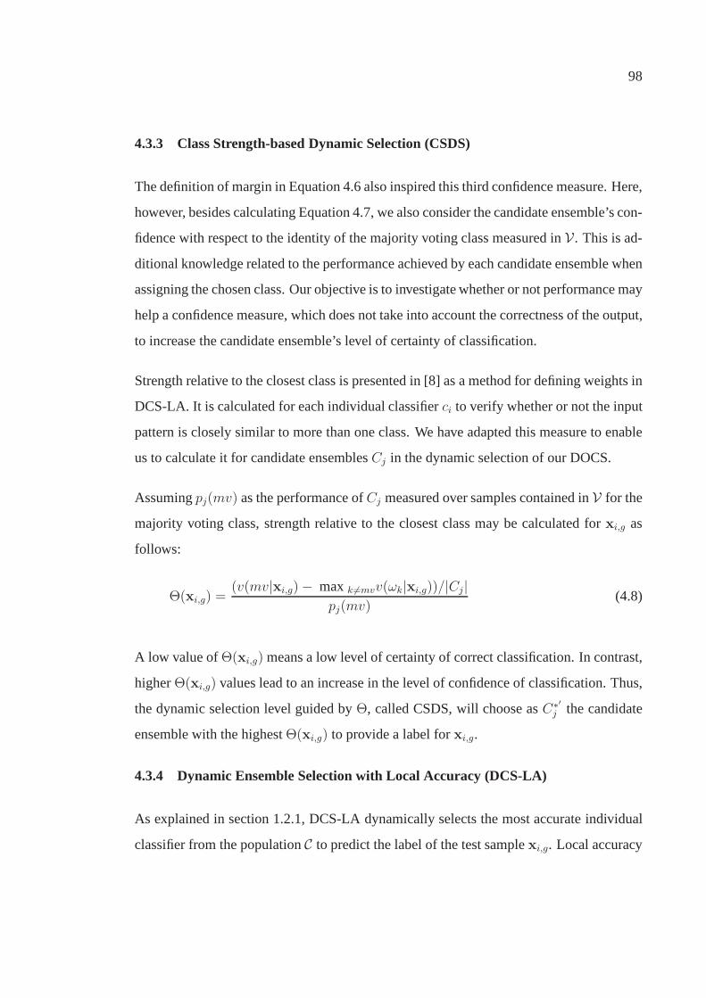
98

4.3.3 Class Strength-based Dynamic Selection (CSDS)

The definition of margin in Equation 4.6 also inspired this third confidence measure. Here,

however, besides calculating Equation 4.7, we also consider the candidate ensemble’s con-

fidence with respect to the identity of the majority voting class measured inV. This is ad-

ditional knowledge related to the performance achieved by each candidate ensemble when

assigning the chosen class. Our objective is to investigatewhether or not performance may

help a confidence measure, which does not take into account the correctness of the output,

to increase the candidate ensemble’s level of certainty of classification.

Strength relative to the closest class is presented in [8] asa method for defining weights in

DCS-LA. It is calculated for each individual classifierci to verify whether or not the input

pattern is closely similar to more than one class. We have adapted this measure to enable

us to calculate it for candidate ensemblesCj in the dynamic selection of our DOCS.

Assumingpj(mv) as the performance ofCj measured over samples contained inV for the

majority voting class, strength relative to the closest class may be calculated forxi,g as

follows:

Θ(xi,g) =(v(mv|xi,g) − maxk 6=mvv(ωk|xi,g))/|Cj|

pj(mv)(4.8)

A low value ofΘ(xi,g) means a low level of certainty of correct classification. In contrast,

higherΘ(xi,g) values lead to an increase in the level of confidence of classification. Thus,

the dynamic selection level guided byΘ, called CSDS, will choose asC∗′j the candidate

ensemble with the highestΘ(xi,g) to provide a label forxi,g.

4.3.4 Dynamic Ensemble Selection with Local Accuracy (DCS-LA)

As explained in section 1.2.1, DCS-LA dynamically selects the most accurate individual

classifier from the populationC to predict the label of the test samplexi,g. Local accuracy

99

is measured in the region of competence composed as the set ofk nearest neighbors fromT

surroundingxi,g. Woods et al. [101] compared two strategies to measure localaccuracy:

(1) overall local accuracy; and (2) local class accuracy. The overall local accuracy is

computed as the number of neighbors correctly classified by each classifierci. However,

in this chapter, we use the second strategy, since Woods et al. have concluded that this is

the strategy that achieves the better results.

Given the poolC and the class assigned by thei-th classifier,ωy, to the test samplexi,g,

we denoteNy as the number of neighbors ofxi,g for which classifierci has correctly

assigned classωy, and∑k

i=1Niy is the total number of neighbors labeled forci as classωy.

According to the definition provided in [101], local class accuracy estimation is computed

as follows:

αci(xi,g) =Ny

∑ki=1N

iy(4.9)

Taking into account that DCS-LA was originally proposed to deal with populations of

classifiers, as summarized in Equation 4.9, it cannot be directly employed in problems in-

volving populations of classifier ensembles. Thus, we propose to change the DCS-LA with

local class accuracy estimation slightly in order to allow it to be used to guide dynamic

selection in our proposed approach. Given a populationC∗′ of candidate ensembles, we

assumeωy as the class assigned by the candidate ensembleCj (composed ofl classifiers)

to the test patternxi,g. We define as region of competence the set of k nearest neighbors

from V surroundingxi,g. Clearly, DCS-LA can be critically affected by the choice ofthe

k parameter. The local candidate ensemble’s class accuracy is then estimated as follows:

αCj(xi,g) =

∑li=1 αci(xi,g)

|Cj|(4.10)

100

To summarize, in this chapter,αCjfor patternxi,g is calculated as the sum of the local class

accuracy (αci) of each classifier composingCj, divided by the size ofCj. The higherαCj,

the greater the certainty of the decision. Table XII shows a summary of the four different

strategies proposed for use at the dynamic selection level of our DOCS.

Table XII

Summary of the four strategies employed at the dynamic selection level. The arrowsspecify whether or not the certainty of the decision is greater if the strategy is lower (↓) or

greater (↑).

Name Label ↑ / ↓Ambiguity-Guided Dynamic Selection ADS (↓)Margin-based Dynamic Selection MDS (↑)Class Strength-based Dynamic Selection CSDS (↑)Dynamic Ensemble Selection with Local Accuracy DCS-LA (↑)

Using the case study mentioned in section 4.2, we compare, inTable XIII, the results

obtained inG using the combination of the initial poolC, SOCS and our DOCS employ-

ing the four dynamic strategies presented in this section. These preliminary results show

that, except for CSDS, our dynamic method guided by confidence measures outperformed

SOCS performed by NSGA-II. In terms of the single-objectiveGA, static and dynamic

selection methods presented similar results, except for CSDS and DCS-LA.

Table XIII

Case study: comparison among the results achieved by combining all classifiers in theinitial pool C and by performing classifier ensemble selection employing both SOCS and

DOCS.

Optimization Combination SOCS ADS MDS CSDS DCS-LANSGA-II (ǫ & θ) 6.06 5.86 5.74 5.71 6.01 5.74GA (ǫ) 6.06 5.90 5.90 5.88 6.13 5.98

101

Figures 20 and 21 show histograms of the frequency of selection of each candidate en-

semble performed using each dynamic selection strategy presented in this section. The

histograms in Figure 20 were obtained for the populationC∗′ composed ofn best candi-

date ensembles generated by GA shown in Figure 18(c), while the histograms in Figure

21 were obtained considering the Pareto front determined byII shown in Figure 18(d).

Especially noteworthy is the fact that the test setG used for the case study is composed

of 12,092 samples (Table VI), even though the dynamic selection level was conducted

over only 325 and 436 of test samples for MOGA and GA respectively. All candidate

ensembles inC∗′ agreed on the label for the remaining test samples.

It is also important to observe in Figure 21 that ADS, MDS and DCS-LA more often

selected asC∗′j the same candidate ensemble selected statically (C1 in Figure 18(d)). In

contrast, the opposite behavior is shown in Figure 20. Theseresults indicate why DOCS

did not outperform SOCS for the GA’s population of candidateensembles (see Table XIII).

In addition, two of the confidence-based dynamic strategies, namely ADS and MDS,

more frequently selected the same candidate ensembles as selected by DCS-LA, which

is an accuracy-oriented strategy. These results support our assumption that selecting the

candidate ensemble with the largest consensus improves theperformance of the system.

Moreover, considering the results obtained by CSDS, we can conclude that measures of

confidence that do not take into account the correctness of the output provide enough in-

formation about a candidate ensemble’s level of certainty of classification. The additional

information calculated by CSDS through measuring the performance of each candidate

ensemble over samples inV did not help in finding better performing ensembles. In next

section, we present experimental results to verify whetheror not these preliminary results

are general, considering other databases and ensemble generation methods.

102

0 1 2 3 4 5 6 7 8 9 10 11 12 13 14 15 16 17 18 19 20 210

10

20

30

40

50

60

70

80

Classifier Label

Sel

ectio

n F

requ

ency

(a) ADS

0 1 2 3 4 5 6 7 8 9 10 11 12 13 14 15 16 17 18 19 20 210

10

20

30

40

50

60

70

80

Classifier Label

Sel

ectio

n F

requ

ency

(b) MDS

0 1 2 3 4 5 6 7 8 9 10 11 12 13 14 15 16 17 18 19 20 210

10

20

30

40

50

60

70

80

Classifier Label

Sel

ectio

n F

requ

ency

(c) CSDS

0 1 2 3 4 5 6 7 8 9 10 11 12 13 14 15 16 17 18 19 20 210

10

20

30

40

50

60

70

80

Classifier Label

Sel

ectio

n F

requ

ency

(d) DCS-LA

Figure 20 Case study: histogram of the frequency of selection of candidate ensemblesperformed by each dynamic selection strategy. The population C

∗′ is thenbest solution generated by GA (see Figure 18(c)).

4.4 Experiments

A series of experiments has been carried out to determine thebest strategy for the dynamic

selection level proposed in our approach and to show whetheror not DOCS is better than

SOCS. As a consequence, we also point out the best method for the overproduction phase

on comparing RSS and BAG, and the best search algorithm and search criteria for the

optimization level. We used seven datasets divided into twogroups: (1) two large; and (2)

103

1 2 3 4 5 6 7 8 9 10 11 120

10

20

30

40

50

60

70

80

90

100

Classifier Label

Sel

ectio

n F

requ

ency

(a) ADS

1 2 3 4 5 6 7 8 9 10 11 120

10

20

30

40

50

60

70

80

90

100

Classifier Label

Sel

ectio

n F

requ

ency

(b) MDS

1 2 3 4 5 6 7 8 9 10 11 120

10

20

30

40

50

60

70

80

90

100

Classifier Label

Sel

ectio

n F

requ

ency

(c) CSDS

1 2 3 4 5 6 7 8 9 10 11 120

10

20

30

40

50

60

70

80

90

100

Classifier Label

Sel

ectio

n F

requ

ency

(d) DCS-LA

Figure 21 Case study: histogram of the frequency of selection of candidate ensemblesperformed by each dynamic selection method. The populationC

∗′ is thePareto front generated by NSGA-II (see Figure 18(d)).

five small, Tables VI and XIV respectively. The datasets fromgroup 1 are the same large

datasets used in chapter 3. Therefore, they are large enoughto be partitioned into the four

independent datasets, illustrated in Figure 17:T , O, V andG using the classical holdout

validation strategy for the evaluation of performance. By contrast, 10-fold cross-validation

is applied for the evaluation of performance using small datasets due to the small number

of samples available for evaluation.

104

Table XIV describes the five small datasets: theDna, satimageandtexture are the same

small datasets used in chapter 3. We used two additional small datasets in this chapter:

feltwell is a multisensor remote-sensing dataset [76] andship is a dataset composed of

forward-looking infra-red (FLIR) ship images [56]. The twonew datasets are traditionally

employed in works dealing with dynamic classifier selection.

Table XIV

Specifications of the small datasets used in the experiments.

Dataset Number of Number of Number of Features PoolCsamples classes features RSS size

Dna 3186 3 180 45 100Feltwell 10944 5 15 8 100Satimage 6435 6 36 18 100Ship 2545 8 11 6 100Texture 5500 11 40 20 100

In this chapter we follow the same experimental protocol employed in chapter 3. To

summarize, for the overproduction phase, three different initial pools of 100 homogeneous

classifiers were created: 100 kNN and 100 DT generated by RSS,and 100 DT generated

by BAG. The selection phase was divided into two levels: for the optimization level, each

diversity measure mentioned in section 3.3.1 was employed in combination withǫ to guide

NSGA-II, while onlyǫ was used to guide single-objective GA. For the dynamic selection

level, all four dynamic strategies defined in section 4.3 were tested so that they could be

compared. We setk = 10 for experiments with DCS-LA, as employed in [84] and [79].

The results obtained are given in subsequent sections.

4.4.1 Comparison of Dynamic Selection Strategies

A summary of the experimental results comparing the four dynamic selection strategies

defined in section 4.3 is given in Tables XV, XVI and XVII. The best result for each

dataset is shown in bold. These results indicate that ADS andMDS were the best strate-

105

Table XV

Mean and standard deviation values obtained on 30 replications of the selection phase ofour method. The overproduction phase was performed using aninitial pool of kNN

classifiers generated by RSS. The best result for each dataset is shown in bold.

Dataset Method NSGA-II GAambiguity coincident difficulty double-fault error

(γ) (σ) (θ) (δ) (ǫ)

DNA

DCS-LA 9.33 (0.27) 9.84 (0.28) 7.48 (0.24) 9.36 (0.30) 7.47 (0.15)ADS 10.31 (0.28) 9.72 (0.47) 7.51 (0.22) 9.30 (0.23) 7.24 (0.21)MDS 10.34 (0.30) 9.57 (0.41) 7.47 (0.21) 9.16 (0.28) 7.24(0.15)CSDS 10.56 (0.30) 9.89 (0.19) 7.48 (0.19) 8.36 (0.30) 7.25 (0.17)

Felwell

DCS-LA 11.17 (0.21) 10.46 (0.25) 9.70(0.14) 10.59 (0.31) 9.87 (0.13)ADS 10.51 (0.11) 10.34 (0.25) 9.82 (0.16) 10.62 (0.28) 9.95 (0.17)MDS 10.51 (0.11) 10.34 (0.26) 9.82 (0.14) 10.59 (0.29) 9.95 (0.16)CSDS 10.57 (0.10) 10.40 (0.25) 9.84 (0.14) 10.66 (0.32) 9.97(0.17)

Nist-digitsTest1

DCS-LA 4.12 (0.07) 4.59 (0.17) 3.72 (0.05) 4.43 (0.26) 3.60 (0.06)ADS 3.80 (0.04) 3.95 (0.05) 3.58 (0.03) 7.49 (2.29) 3.53 (0.05)MDS 3.80 (0.04) 3.94 (0.05) 3.58 (0.02) 7.46 (2.32) 3.53(0.05)CSDS 5.21 (0.09) 7.25 (0.26) 3.80 (0.04) 6.67 (0.22) 3.80 (0.06)

Nist-digitsTest2

DCS-LA 8.57 (0.14) 9.34 (0.28) 8.18 (0.11) 9.48 (0.43) 7.91 (0.10)ADS 8.11 (0.06) 8.55 (0.08) 7.97 (0.05) 8.40 (0.48) 7.78(0.10)MDS 8.12 (0.07) 8.53 (0.09) 7.97 (0.05) 8.36 (0.55) 7.78 (0.10)CSDS 9.95 (0.11) 9.89 (0.33) 8.21 (0.08) 9.42 (0.45) 8.09 (0.10)

Nist-letters

DCS-LA 7.63 (0.43) 8.22 (0.69) 6.48 (0.15) 7.20 (0.33) 6.55 (0.16)ADS 7.23 (0.17) 8.22 (0.12) 6.48 (0.07) 6.95 (0.12) 6.43 (0.06)MDS 7.16 (0.16) 7.07 (0.11) 6.27(0.07) 6.88 (0.12) 6.41 (0.08)CSDS 10.15 (0.45) 14.53 (0.63) 6.47 (0.14) 9.35 (0.41) 6.70 (0.09)

Satimage

DCS-LA 8.75 (0.08) 9.60 (0.15) 8.73 (0.13) 9.40 (0.13) 8.63 (0.07)ADS 8.67 (0.08) 9.05 (0.17) 8.64 (0.13) 9.16 (0.16) 8.61(0.09)MDS 8.68 (0.09) 9.04 (0.18) 8.65 (0.14) 9.16 (0.18) 8.61 (0.09)CSDS 8.96 (0.13) 10.13 (0.24) 8.80 (0.16) 9.78 (0.19) 8.67 (0.11)

Ship

DCS-LA 14.24 (0.32) 10.31 (0.29) 9.34 (0.24) 9.24 (0.23) 10.40 (0.20)ADS 13.25 (0.24) 9.60 (0.33) 9.25 (0.20) 9.13(0.21) 9.81 (0.16)MDS 13.37 (0.26) 9.66 (0.31) 9.24 (0.20) 9.15 (0.22) 9.83 (0.13)CSDS 14.06 (0.25) 10.17 (0.34) 9.39 (0.21) 9.31 (0.29) 10.23(0.18)

Texture

DCS-LA 1.51 (0.06) 1.64 (0.08) 0.97 (0.05) 1.02 (0.07) 1.18 (0.03)ADS 1.37 (0.05) 1.23 (0.09) 0.94(0.05) 0.98 (0.07) 1.11 (0.01)MDS 1.37 (0.05) 1.22 (0.09) 0.94 (0.05) 0.98 (0.07) 1.11 (0.02)CSDS 1.37 (0.07) 1.28 (0.10) 0.94 (0.06) 0.98 (0.09) 1.11 (0.03)

gies for performing the dynamic selection level of our approach, considering all three

ensemble creation methods investigated, i.e. (1) ensembleof kNN; (2) ensemble of DT

generated through RSS (Tables XV and XVI); and (3) ensemblesof DT generated by BAG

106

Table XVI

Mean and standard deviation values obtained on 30 replications of the selection phase ofour method. The overproduction phase was performed using aninitial pool of DT

classifiers generated by RSS. The best result for each dataset is shown in bold.

Dataset Method NSGA-II GAambiguity coincident difficulty double-fault error

(γ) (σ) (θ) (δ) (ǫ)

DNA

DCS-LA 7.05 (0.21) 7.54 (0.28) 4.63 (0.15) 7.23 (0.23) 5.14 (0.14)ADS 7.94 (0.23) 6.50 (0.29) 4.59(0.17) 6.27 (0.23) 4.95 (0.18)MDS 7.92 (0.23) 6.54 (0.30) 4.63 (0.17) 6.27 (0.19) 4.92 (0.19)CSDS 8.01 (0.24) 6.59 (0.28) 4.62 (0.17) 6.34 (0.22) 4.93 (0.19)

Felwell

DCS-LA 12.68 (0.19) 13.27 (0.47) 11.65 (0.32) 12.79 (0.51) 11.59 (0.14)ADS 11.60 (0.15) 12.71 (0.40) 11.65 (0.33) 12.51 (0.51)11.50(0.17)MDS 11.59 (0.14) 12.74 (0.42) 11.65 (0.32) 12.49 (0.48) 11.53 (0.16)CSDS 11.66 (0.15) 12.80 (0.43) 11.65 (0.32) 12.51 (0.50) 11.51 (0.16)

Nist-digitsTest1

DCS-LA 3.82 (0.12) 5.37 (0.29) 2.91 (0.04) 3.68 (0.20) 2.89 (0.04)ADS 3.35 (0.04) 4.11 (0.20) 2.77(0.03) 3.59 (0.23) 2.77(0.09)MDS 3.35 (0.04) 3.83 (0.13) 2.77 (0.02) 3.40 (0.12) 2.77 (0.04)CSDS 5.63 (0.09) 5.53 (0.12) 2.98 (0.06) 4.47 (0.78) 3.12 (0.06)

Nist-digitsTest2

DCS-LA 8.18 (0.18) 10.06 (0.50) 6.79 (0.09) 8.07 (0.37) 6.66(0.08)ADS 7.38 (0.07) 9.16 (0.32) 6.45(0.05) 8.11 (0.40) 6.45(0.05)MDS 7.34 (0.06) 8.61 (0.20) 6.50 (0.05) 7.80 (0.20) 6.45 (0.05)CSDS 9.05 (0.14) 8.77 (0.54) 6.50 (0.09) 8.69 (0.50) 6.98 (0.10)

Nist-letters

DCS-LA 7.57 (0.30) 6.12 (0.50) 6.03 (0.14) 7.20 (0.39) 6.17 (0.14)ADS 7.13 (0.09) 9.31 (0.29) 5.84(0.06) 7.12 (0.14) 5.96 (0.06)MDS 7.12 (0.09) 7.69 (0.19) 5.84 (0.06) 6.93 (0.10) 5.95 (0.06)CSDS 10.65 (0.11) 15.92 (0.14) 5.98 (0.08) 10.95 (0.46) 6.29(0.09)

Satimage

DCS-LA 9.30 (0.09) 10.66 (0.19) 8.97 (0.09) 10.12 (0.15) 8.96 (0.09)ADS 8.73 (0.10) 9.22 (0.19) 8.64 (0.10) 9.17 (0.15) 8.78 (0.12)MDS 8.73 (0.10) 9.22 (0.19) 8.63(0.09) 9.16 (0.15) 8.77 (0.13)CSDS 9.13 (0.13) 11.23 (0.24) 8.94 (0.12) 10.64 (0.26) 8.86 (0.12)

Ship

DCS-LA 10.65 (0.30) 9.16 (0.30) 7.53 (0.18) 7.93 (0.29) 7.24(0.14)ADS 8.86 (0.25) 8.26 (0.34) 7.17 (0.15) 7.72 (0.28) 6.98 (0.14)MDS 8.94 (0.26) 8.26 (0.32) 7.18 (0.15) 7.75 (0.29) 6.95(0.13)CSDS 9.97 (0.24) 9.15 (0.41) 7.18 (0.17) 8.03 (0.27) 7.35 (0.12)

Texture

DCS-LA 3.42 (0.17) 3.85 (0.14) 2.47 (0.07) 3.51 (0.16) 2.84 (0.09)ADS 2.98 (0.08) 3.02 (0.14) 2.35(0.06) 2.97 (0.14) 2.44) (0.05MDS 3.00 (0.08) 3.04 (0.14) 2.35 (0.05) 2.65 (0.16) 2.44 (0.05)CSDS 3.01 (0.08) 3.06 (0.15) 2.35 (0.05) 2.96 (0.16) 2.44 (0.06)

(Table XVII). These two dynamic strategies presented equivalent performances, which

confirms the preliminary results in our case-study problem (see Table XIII). CSDS was

the worst dynamic selection strategy for 1 and 3, while DCS-LA was most likely to be the

107

Table XVII

Mean and standard deviation values obtained on 30 replications of the selection phase ofour method. The overproduction phase was performed using aninitial pool of DTclassifiers generated by Bagging. The best result for each dataset is shown in bold.

Dataset Method NSGA-II GAambiguity coincident difficulty double-fault error

(γ) (σ) (θ) (δ) (ǫ)

DNA

DCS-LA 5.15 (0.15) 5.20 (0.18) 4.75(0.15) 5.30 (0.15) 4.88 (0.09)ADS 5.20 (0.16) 5.20 (0.16) 4.86 (0.11) 5.32 (0.21) 4.95 (0.06)MDS 5.17 (0.17) 5.20 (0.18) 4.86 (0.10) 5.31 (0.23) 4.95 (0.06)CSDS 5.19 (0.15) 5.22 (0.17) 4.86 (0.11) 5.36 (0.25) 4.97 (0.07)

Felwell

DCS-LA 12.50 (0.36) 12.47 (0.28) 12.00 (0.22) 12.40 (0.32)11.69(0.20)ADS 12.70 (0.21) 12.28 (0.34) 12.04 (0.18) 12.24 (0.31) 11.95 (0.14)MDS 12.70 (0.17) 12.28 (0.35) 12.03 (0.18) 12.24 (0.29) 11.94 (0.14)CSDS 12.75 (0.19) 12.38 (0.33) 12.04 (0.19) 12.34 (0.32) 11.98 (0.15)

Nist-digitsTest1

DCS-LA 5.74 (0.09) 6.72 (0.36) 5.67 (0.09) 6.04 (0.21) 5.23 (0.06)ADS 5.53 (0.05) 5.79 (0.11) 5.51 (0.05) 5.47 (0.10) 5.14(0.06)MDS 5.52 (0.05) 5.69 (0.10) 5.51 (0.05) 5.44 (0.09) 5.14 (0.05)CSDS 5.87 (0.12) 6.86 (0.56) 5.64 (0.09) 6.72 (0.41) 5.44 (0.06)

Nist-digitsTest2

DCS-LA 11.00 (0.16) 11.60 (0.55) 10.98 (0.15) 10.64 (0.37) 10.21 (0.12)ADS 10.71 (0.09) 10.81 (0.25) 10.71 (0.09) 10.59 (0.18)10.06(0.11)MDS 10.70 (0.09) 11.02 (0.24) 10.70 (0.10) 10.54 (0.12) 10.06 (0.10)CSDS 11.18 (0.20) 12.76 (0.91) 10.88 (0.12) 11.68 (0.61) 10.41 (0.11)

Nist-letters

DCS-LA 7.81 (0.17) 9.13 (0.62) 7.64 (0.12) 8.45 (0.44) 7.79 (0.12)ADS 7.61 (0.06) 8.36 (0.15) 7.50(0.06) 8.06 (0.17) 7.64 (0.07)MDS 7.63 (0.06) 8.30 (0.10) 7.50 (0.05) 8.02 (0.14) 7.64 (0.07)CSDS 7.85 (0.07) 10.16 (0.94) 7.60 (0.08) 9.84 (0.54) 7.78 (0.01)

Satimage

DCS-LA 9.70 (0.38) 11.35 (0.57) 9.81 (0.11) 10.99 (0.22) 9.74 (0.09)ADS 9.34 (0.43) 10.36 (0.60) 9.62 (0.09) 10.25 (0.13) 9.61 (0.11)MDS 9.21(0.37) 10.44 (0.58) 9.63 (0.07) 10.22 (0.11) 9.61 (0.12)CSDS 9.78 (0.17) 12.08 (0.22) 9.78 (0.11) 11.82 (0.28) 9.68 (0.12)

Ship

DCS-LA 7.79 (0.19) 8.32 (0.29) 7.81 (0.29) 8.58 (0.29) 7.72(0.13)ADS 8.14 (0.20) 8.70 (0.29) 8.36 (0.19) 8.83 (0.27) 8.07 (0.09MDS 8.16 (0.20) 8.71 (0.29) 8.38 (0.17) 8.84 (0.28) 8.05 (0.09)CSDS 8.46 (0.23) 9.04 (0.32) 8.53 (0.21) 9.12 (0.27) 8.15 (0.16)

Texture

DCS-LA 3.69 (0.09) 4.40 (0.43) 3.44 (0.09) 4.17 (0.13) 3.66 (0.07)ADS 3.57 (0.09) 4.02 (0.56) 3.41(0.008) 4.03 (0.15) 3.60 (0.06)MDS 3.56 (0.09) 3.93 (0.63) 3.42 (0.08) 4.04 (0.15) 3.60 (0.06)CSDS 3.63 (0.10) 4.01 (0.18) 3.43 (0.11) 3.43 (0.11) 3.58 (0.08)

worst dynamic selection strategy for ensembles of DT generated by RSS. In terms of the

optimization level, single-objective GA and NSGA-II presented equivalent performances

for ensembles of kNN generated by RSS and ensembles of DT generated by BAG, while

108

NSGA-II found the best results for populations of ensemblesof DT generated by RSS.θ

was clearly the best diversity measure for composing, withǫ, a pair of objective functions

to guide NSGA-II, whileγ andσ were the worst diversity measures.

It is important to note that DCS-LA was better than the other dynamic selection strategies

in 3 of the 8 datasets in problems involving DT generated by BAG. The reason for this

behavior is that BAG provides the complete representation of the problem to each classifier

member, whereas RSS provides only a partial representation. Thus, DCS-LA calculates

the local accuracy of each classifier more accurately when BAG is used as the ensemble

creation method. Also important is the fact that CSDS was less effective in problems

involving a large number of classes, such asNIST-letters, because it takes into account

the performance of the candidate ensembles for each class involved in the classification

problem, in addition to the extent of consensus of the ensembles. Moreover, for the same

reason, CSDS is much more critically affected by the qualityof the population of candidate

ensembles found at the optimization level. For instance, sinceγ andσ were the worst

objective functions when guiding the optimization level, CSDS was much worse than

the other three strategies when used to perform the dynamic selection on populations of

candidate ensembles found by these two diversity measures.

4.4.2 Comparison between DOCS and Several Methods

In this section, we summarize the best results obtained by our DOCS for each dataset, in

order to show that the proposed approach outperforms other related methods. Table XVIII

reports the results attained by the following methods:

• Fusion of the initial pool of classifiersC by majority voting;

• Selection of the best individual classifier from the initialpoolC;

• Individual kNNs and DTs trained using all available features;

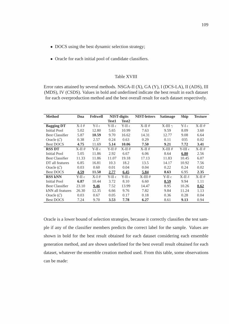
109

• DOCS using the best dynamic selection strategy;

• Oracle for each initial pool of candidate classifiers.

Table XVIII

Error rates attained by several methods. NSGA-II (X), GA (Y), I (DCS-LA), II (ADS), III(MDS), IV (CSDS). Values in bold and underlined indicate thebest result in each datasetfor each overproduction method and the best overall result for each dataset respectively.

Method Dna Feltwell NIST-digits NIST-letters Satimage Ship TextureTest1 Test2

Bagging DT X-I θ Y-I ǫ Y-II ǫ Y-II ǫ X-II θ X-III γ Y-I ǫ X-II θInitial Pool 5.02 12.80 5.65 10.99 7.63 9.59 8.09 3.60Best Classifier 5.87 10.59 9.70 16.62 14.31 12.77 9.08 6.64Oracle (C) 0.38 2.57 0.24 0.63 0.29 0.11 035 0.02Best DOCS 4.75 11.69 5.14 10.06 7.50 9.21 7.72 3.41RSS DT X-II θ Y-II ǫ Y-II θ X-II θ X-II θ X-III θ Y-III ǫ X-II θInitial Pool 5.05 11.86 2.92 6.67 6.06 8.64 6.80 2.56Best Classifier 11.33 11.86 11.07 19.18 17.13 11.83 10.45 6.07DT all features 6.85 16.81 10.3 18.2 13.5 14.17 10.92 7.56Oracle (C) 0.03 0.60 0.01 0.04 0.04 0.22 0.24 0.02Best DOCS 4.59 11.50 2.77 6.45 5.84 8.63 6.95 2.35RSS kNN Y-II ǫ X-I θ Y-II ǫ Y-II ǫ X-III θ Y-II ǫ X-II δ X-II θInitial Pool 6.87 10.44 3.72 8.10 6.60 8.59 9.94 1.11Best Classifier 23.10 9.46 7.52 13.99 14.47 8.95 10.26 0.62kNN all features 26.30 12.35 6.66 9.76 7.82 9.84 11.24 1.13Oracle (C) 0.03 0.67 0.05 0.17 0.18 0.36 0.28 0.04Best DOCS 7.24 9.70 3.53 7.78 6.27 8.61 9.13 0.94

Oracle is a lower bound of selection strategies, because it correctly classifies the test sam-

ple if any of the classifier members predicts the correct label for the sample. Values are

shown in bold for the best result obtained for each dataset considering each ensemble

generation method, and are shown underlined for the best overall result obtained for each

dataset, whatever the ensemble creation method used. From this table, some observations

can be made:

110

• Analyzing the results obtained for ensembles of DT generated using BAG, our

DOCS outperformed the other methods, except forfeltwell. The same scenario

was observed for ensembles of DT generated using RSS, but theexception was the

ship dataset. For ensembles of kNN generated using RSS, however,the proposed

method outperformed the other methods in only 4 of the 8 cases. For the remaining

4 datasets, our DOCS was the second best method. The combination of the initial

poolC was the best method fordna andsatimagewhile the individual best classifier

from C was the best method forfeltwell andtexture.

• Confidence-based dynamic strategies were better than DCS-LA for performing the

dynamic selection of the selection phase. Even though ADS and MDS presented

similar behavior, we show in Table XVIII values obtained using ADS to perform

the comparison in next section.

• The search algorithms presented equivalent performances.The best results found

using DOCS were obtained in populations of candidate ensembles optimized by

NSGA-II in 13 cases and by single-objective GA in 11 cases outof a total of 24

cases investigated.

• θ was the best diversity measure for combining withǫ to guide NSGA-II.

• RSS was better than BAG for use during the overproduction phase. Results obtained

using ensembles generated by RSS were both better than thoseobtained using en-

sembles generated by BAG.

• DT was the best classifier model to be used as a base classifier during the overpro-

duction phase. Five of the best overall results were obtained with ensembles of DT,

whereas in the remaining three datasets they were obtained with ensembles of kNN.

Both ensembles were generated by RSS.

111

Table XIX presents some of the results reported in the literature dealing with the selection

of classifiers, except for references [32] and [66], on the databases used in this chapter. In

this way, it is possible to gain an overview of the results obtained in the literature, even

though the method of partition of the data used in some of these works was not the same

as that used in this chapter.

Table XIX

The error rates obtained, the data partition and the selection method employed in workswhich used the databases investigated in this chapter (FSS:feature subset selection).

Database Reference Ensemble Classifiers Partition Selection ErrorNumber Creation Members Strategy Type (%)

Dna [32] RSS DT Holdout Fusion 9.19Feltwell [15] Het Het Cross-validation DCS-LA 13.62NIST-digits Test1 [89] RSS kNN Holdout SOCS 3.65NIST-letters [61] FSS MLP Holdout SOCS 4.02Satimage [15] Het Het Cross-validation DCS-LA 10.82Ship [66] Het Het Holdout Fusion 5.68Texture [101] DT Het Holdout DCS-LA 0.75

To verify whether or not our DOCS is better that the classicalSOCS, in the next section,

we concentrate our analysis on the methods that attained thebest results in this section,

i.e. DT ensembles generated by RSS, ADS as dynamic strategy;MOGA guided byθ in

combination withǫ; and GA guided byǫ.

4.4.3 Comparison of DOCS and SOCS Results

The static selection results were obtained by picking up thecandidate ensemble presenting

the lowestǫ value of all the solutions composing then best solution (for single-objective

GA) or the Pareto front (for NSGA-II). These ensembles are represented in Figures 18(c)

and 18(d) by black circles. It is important to mention that the results were tested on mul-

tiple comparisons using the Kruskal-Wallis nonparametricstatistical and the confidence

level was 95% (α = 0.05), as was done in previous chapters.

112

Table XX summarizes the mean and the standard deviation of the error rates obtained on

all eight databases comparing the static and dynamic OCS. These results indicate, without

exception, that our DOCS was better than the traditional SOCS. In two specific situations

(feltwell andNIST-letters), the differences between the two methods were not significant.

It is important to note that the results achieved using NSGA-II guided by bothθ and ǫ

outperformed the results found using GA guided byǫ the single-objective function. This

is a different result from those presented in [72] and [89]. It appears that performing

dynamic selection in the selection phase resulted in exploiting all possible potentials of

the population of candidate ensembles over the Pareto front, leading to more benefits for

NSGA-II with the new level. However, only with thetexture database was GA better than

NSGA-II in SOCS, whereas in DOCS the opposite is true.

Table XX

Mean and standard deviation values of the error rates obtained on 30 replicationscomparing DOCS and SOCS with no rejection. Values in bold indicate the lowest error

rate and underlined when a method is significantly better than the others.

Dataset SOCS DOCSNSGA-II (θ & ǫ) GA ǫ NSGA-II (θ & ǫ) GA ǫ

Dna 4.77 (0.17) 4.97 (0.16) 4.59(0.17) 4.95 (0.19)Feltwell 12.02 (0.38) 11.86 (0.06) 11.65 (0.33) 11.50(0.17)NIST-digits Test1 2.82 (0.06) 2.84 (0.06) 2.77(0.03) 2.77(0.03)NIST-digits Test2 6.59 (0.09) 6.53 (0.09) 6.45(0.05) 6.45(0.05)NISt-letters 5.89 (0.07) 6.02 (0.09) 5.84(0.06) 5.96 (0.06)Satimage 8.76 (0.13) 8.82 (0.12) 8.64(0.10) 8.78 (0.12)Ship 7.35 (0.17) 7.14 (0.23) 7.17 (0.15) 6.98(0.14)Texture 2.41 (0.09) 2.51 (0.09) 2.35(0.06) 2.44 (0.05)

All these results were obtained with a zero reject rate. However, as advocated by Hansen

et al. [29], the reject mechanism for an ensemble of classifiers is based on the extent of

consensus among its members. This means that the decision toreject a pattern is related

to the confidence level of the ensemble. They assume that it isbetter to reject the pattern

if the ensemble presents a low confidence level to take a decision. Such a confidence level

113

is clearly related toγ (Equation 4.4), which is used to guide ADS. Thus, sinceγ is the

criterion used to perform the reject mechanism, we might assume that the difference be-

tween SOCS and DOCS will increase as the rejection rate increases. We analyze such an

assumption in Figure 22 taking into account the case study problem investigated through-

out this chapter. This preliminary result does not confirm this assumption. Both the static

and the dynamic OCS presented similar error-reject curves for ensembles generated by

GA 22(a) and NSGA-II 22(b).

0% 5 % 10% 15% 20% 25% 30% 35% 40% 45% 50%0

1

2

3

4

5

6

Reject

Err

or

SOCSDOCS

(a) GA

0% 5% 10% 15% 20% 25% 30% 35% 40% 45% 50%0

1

2

3

4

5

6

Reject

Err

or

SOCSDOCS

(b) MOGA

Figure 22 Case Study: Error-reject curves for GA (22(a)) andNSGA-II (22(b)).

In order to show more general results about the error-rejecttradeoff, we fixed four different

reject rates: 0.5% and 1.0% (Table XXI), 5.0% and 10.0% (Table XXII), to investigate all

the problems dealt with in this chapter. These results confirm that we should not assume

that DOCS is more effective than SOCS when increasing the rejection rate.

4.5 Discussion

We propose a dynamic overproduce-and-choose strategy which is composed of the tradi-

tional overproduction and selection phases. The novelty isto divide the selection phase

into two levels: optimization and dynamic selection, conducting the second level using

114

Table XXI

Mean and standard deviation values of the error rates obtained on 30 replicationscomparing DOCS and SOCS with rejection. Values in bold indicate the lowest error rate

attained and underlined when a method is significantly better than the others.

Dataset SOCS DOCSNSGA-II (θ & ǫ) GA ǫ NSGA-II (θ & ǫ) GA ǫ

0.5%-rejectionDna 4.50 (0.18) 4.72 (0.18) 4.38(0.19) 4.78 (0.18)Feltwell 11.79 (0.38) 11.62 (0.24) 11.42 (0.33) 11.29(0.17)NIST-digits Test1 2.55 (0.06) 2.55 (0.06) 2.52(0.04) 2.53 (0.03)NIST-digits Test2 6.32 (0.10) 6.26 (0.08) 6.25 (0.05) 6.20(0.06)NIST-letters 5.60 (0.09) 5.71 (0.11) 5.53(0.07) 5.67 (0.06)Satimage 8.52 (0.13) 8.58 (0.13) 8.44(0.09) 8.54 (0.12)Ship 7.06 (0.17) 6.89 (0.24) 6.88 (0.18) 6.87(0.16)Texture 2.22 (0.10) 2.26 (0.09) 2.17(0.06) 2.25 (0.06)

1.0%-rejectionDna 4.29 (0.17) 4.54 (0.20) 4.22(0.18) 4.63 (0.19)Feltwell 11.53 (0.37) 11.38 (0.23) 11.14 (0.33) 11.08(0.17)NIST-digits Test1 2.30(0.06) 2.34 (0.06) 2.31 (0.04) 2.34 (0.03)NIST-digits Test2 6.04 (0.10) 5.99 (0.11) 6.09 (0.07) 5.97(0.06)NIST-letters 5.27 (0.08) 5.41 (0.11) 5.24(0.06) 5.41 (0.07)Satimage 8.31 (0.13) 8.38 (0.14) 8.24(0.11) 8.34 (0.12)Ship 6.74 (0.18) 6.59 (0.21) 6.57 (0.18) 6.52(0.17)Texture 2.04 (0.09) 2.07 (0.09) 2.01(0.06) 2.06 (0.05)

confidence measures based on the extent of consensus of ensembles. The two classical

ensemble creation methods, the random subspace method and bagging, were used for the

overproduction phase, while single- and multi-objective GAs were used at the optimization

level. The ensemble error rates and diversity measures guided the optimization. Finally,

three confidence measures were applied at the dynamic selection level: (1) ambiguity; (2)

margin; and (3) strength relative to the closest class. In addition, DCS-LA was compared

to the confidence-based strategies.

Experiments conducted using eight datasets demonstrated that the proposed approach out-

performs both static selection and the fusion of the initialpool of classifiers. Ambiguity

and margin were the best measures to use at the dynamic selection level, presenting equiva-

115

Table XXII

Mean and standard deviation values of the error rates obtained on 30 replicationscomparing DOCS and SOCS with rejection. Values in bold indicate the lowest error rate

attained and underlined when a method is significantly better than the others.

Dataset SOCS DOCSNSGA-II (θ & ǫ) GA ǫ NSGA-II (θ & ǫ) GA ǫ

5.0%-rejectionDna 3.13(0.15) 3.37 (0.14) 3.18 (0.17) 3.54 (0.16)Feltwell 9.70 (0.35) 9.46 (0.22) 9.48 (0.36) 9.26(0.20)NIST-digits Test1 1.21(0.05) 1.22 (0.04) 1.24 (0.05) 1.29 (0.02)NIST-digits test2 4.38 (0.14) 4.34(0.10) 4.41 (0.10) 4.44 (0.08)NIST-letters 3.64(0.11) 3.79 (0.10) 3.64(0.09) 3.83 (0.06)Satimage 6.72 (0.13) 6.71 (0.12) 6.68(0.12) 6.71 (0.11)Ship 5.05 (0.21) 4.99(0.17) 5.05 (0.16) 5.16 (0.17)Texture 1.01 (0.05) 1.03 (0.05) 0.98(0.07) 1.04 (0.04)

10.0%-rejectionDna 2.06 (0.18) 2.14 (0.18) 2.05(0.19) 2.36 (0.13)Feltwell 7.45 (0.40) 7.50 (0.20) 7.51 (0.29) 7.39(0.22)NIST-digits Test1 0.54(0.03) 0.56 (0.04) 0.54 (0.03) 0.58 (0.03)NIST-digits Test2 2.83(0.10) 2.83(0.10) 2.89 (0.09) 2.93 (0.09)NIST-letters 2.27(0.07) 2.30 (0.08) 2.31 (0.08) 2.42 (0.05)Satimage 5.05 (0.10) 5.02 (0.09) 5.02 (0.10) 4.98(0.09)Ship 3.59(0.13) 3.62 (0.11) 3.64 (0.14) 3.79 (0.12)Texture 0.39 (0.05) 0.37 (0.03) 0.37 (0.05) 0.36(0.04)

lent performances. It was shown that NSGA-II guided by the difficulty measure combined

with the error rate found better ensembles than single-objective GA guided only by the er-

ror rate. In addition, although not as clearly as one might have hoped, our results indicate

that our method is especially valuable for tasks using NSGA-II, since differences between

the results found using NSGA-II and GA are greater in the dynamic than in the static

overproduce-and-choose strategy. Ideally, we should exploit all the potential of the pop-

ulation of candidate ensembles over a Pareto front using theproposed dynamic selection

level.

However, the quality of the population of candidate ensembles found at the optimization

level critically affects the performance of our approach. We can confirm this observation

116

taking into account the concept of oracle. As mentioned before, the so-called oracle is a

lower bound of selection strategies. Table XXIII shows results attained by the fusion of the

initial pool of classifiersC and its oracle for the same case study investigated throughout

this chapter. Only NSGA-II guided byθ combined withǫ is considered in this example.

Table XXIII

Case study: comparing oracle results.

Fusion of Oracle of SOCS DOCS Oracle of populationinitial pool C initial pool C of ensemblesC∗

′

6.06 0.04 5.86 5.71 4.81

It is important to mention that, instead ofC, the Pareto front (population of ensemblesC∗′)

is the input to our dynamic selection level. Hence, we shouldconsider the oracle of the

populationC∗′ as the lower bound for our DOCS. Thus, it is assumed that oracle correctly

classifies the test sample if any of candidate ensembles inC∗′ predicts the correct label for

the sample. In Table XXIII, it is shown that our DOCS may not achieve an error rate lower

than4.81. The large difference between the results of theC andC∗′ oracles leads us to

conclude that there is a major loss of oracle power at the optimization level. Populations

of candidate ensembles with oracle error rates closer to those obtained usingC will bring

about an effective improvement in the performances attained by our method.

CONCLUSION

The focus of this thesis was the selection of classifier ensembles. Our efforts were concen-

trated towards the overproduction-and-choose strategy. We have seen that this strategy is

classically composed of the overproduction and selection phases. While the overproduc-

tion phase may be performed using any ensemble constructionstrategy and base classifier

model, the selection phase is the main challenge in the overproduction-and-choose strat-

egy, since it focuses on finding the best performing subset ofclassifiers. We have called

this approach static overproduction-and-choose strategydue to the fact that the candidate

ensemble selected as the best performing subset of classifiers is used to classify the whole

test dataset.

In our first investigation we analyzed the search criterion,which is one of the two main as-

pects that should be analyzed when the selection phase performs an optimization process

conducted by non-exhaustive search algorithms. Single- and multi-objective optimiza-

tion processes were conducted using GAs. NSGA-II was the multi-objective GA used (in

appendix 1 we show experimental results which support our choice). Fourteen different

objective functions were applied: 12 diversity measures, the error rate and ensemble size,

while an ensemble of 100 kNN classifiers generated using the random subspace method

was used as the initial pool of classifiers created at the overproduction phase. The re-

sults of our experiments have shown that diversity alone cannot be better than the error

rate at finding the most accurate classifier ensembles. However, when both the error rate

and diversity are combined in a multi-objective approach, we observed that the perfor-

mance of the solutions found using diversity is much higher than the performance of the

solutions found using diversity in a single-objective optimization approach. Finally, we

showed that it can be established an analogy between featuresubset selection and static

overproduction-and-choose strategy by combining ensemble size and the error rate in a

pair of objective functions. However, we observed that the reduction in the number of

classifiers is a consequence of the selection process, then,it is not necessary to include

118

explicitly ensemble size in the optimization process. Moreover, our experiments showed

that ensemble size and diversity are not conflicting objective functions, and should not

be used combined to guide the optimization process in a multi-objective approach. This

observation, which is also confirmed in appendix 3, leads to the conclusion that the results

obtained using single-objective GA in our experiments may be different if the minimum

number of classifiers is fixed and larger than we have defined inchapter 2.

We then proceeded to investigate the problem of overfitting detected at the optimization

process of the selection phase. We presented three overfitting control methods: (1) partial

validation; (2) backwarding; and (3) global validation. Three initial pools of 100 classifiers

were generated: 100 kNN and 100 Decision Trees using the random subspace method, and

a third pool of 100 Decision Trees using bagging. Five different objective functions were

applied: four diversity measures and the error rate were used to guide both single- and

multi-objective GAs. We confirmed that overfitting can be detected at the selection phase,

especially when NSGA-II is employed as the search algorithm. Global validation out-

performed the other overfitting control methods, while random subspace-based ensembles

were more prone to overfitting than bagging-based ones. We also proposed to use global

validation as a tool for identifying the diversity measure most closely related to perfor-

mance. Our results indicated that double-fault was the diversity measure more closely

related to performance. In addition, we showed that the difficulty measure can be better

than the error rate as a single-objective function for selecting high-performance ensem-

bles of classifiers. However, taking into account our previous experimental results, which

show that the minimum number of classifiers is achieved when using most of the diversity

measures in single-objective optimization, quite a large minimum ensemble size was fixed

in our experiments. Therefore, these results are still dependent of the minimum ensemble

size defined.

Lastly, we have proposed a dynamic overproduce-and-choosestrategy which combines

optimization and dynamic selection in a two-level selection phase to allow the selection of

119

the most confident subset of classifiers to label each test sample individually. In this way,

instead of choosing only one solution to classify the whole test dataset, all potential high

accuracy candidate ensembles from the population generated by the search algorithms,

are considered to select the most competent solution for each test sample. Moreover, we

proposed to conduct our dynamic selection level using confidence measures based on the

extent of consensus of candidate ensembles. These measureslead to the selection of the

solution with the highest level of confidence among its members, allowing an increase

in the “degree of certainty" of the classification. The same three initial pools of classi-

fiers, generated by the random subspace method and bagging, were used as output of the

overproduction phase. Single- and multi-objective GAs guided by the same five objective

functions, i.e. four diversity measures and the error rate,were used at the optimization

level. Finally, three different confidence measures were proposed to be used at the dy-

namic selection level.

Our experiments, which were carried out on eight real classification problems in-

cluding handwritten digits and letters, texture, multisensor remote-sensing images and

forward-looking infra-red ship images, demonstrated thatour method outperforms static

overproduce-and-choose strategy, a classical dynamic classifier selection method and the

combination of the decisions of the classifiers in the initial pools. In despite of these per-

formance improvements, we observed that the quality of the population of candidate en-

sembles found at the optimization level critically affectsthe performance of our approach.

Still more interesting is the observed major loss of oracle power at the optimization level.

Taking into account that oracle is the lower bound of selection strategies, the optimiza-

tion level of our method increases the lower bound, consequently avoiding the dynamic

selection level to attain more effective improvement in theperformances.

120

Future Works

Even though this thesis successfully investigated the static overproduce-and-choose strat-

egy and proposed a dynamic overproduce-and-choose strategy, some issues were not ad-

dressed owing to time. The following future directions are possible and worthy of investi-

gation:

• Determine strategies to improve the quality of the population of ensembles. We

believe that the optimization level can be improved in orderto decrease the lower

bound oracle for our dynamic overproduce-and-choose strategy.

• Investigate different strategies for the generation of thepopulation of classifier en-

sembles, which is the input of the dynamic selection level ofour method.

• Develop new confidence measures focusing on increasing the confidence of the de-

cisions.

• Investigate the impact of our dynamic overproduce-and-choose strategy in problems

involving missing features.

APPENDIX 1

Comparison of Multi-Objective Genetic Algorithms

122

Genetic Algorithms are the population-based search algorithms investigated in this thesis.

In chapter 2 we mentioned that single- and multi-objective GAs are two possible options

when dealing with GAs. Three MOGAs were investigated in order to allow us to define

the best option to be used in all the experiments conducted inthis thesis. The following

three MOGAs were investigated: (1) Non-dominated sorting GA (NSGA) [11]; (2) Fast

elitist non-dominated sorting GA (NSGA-II) [13]; and (3) controlled elitist NSGA [14].

The general GA parameters presented in Table V, chapter 2, are used for all three MOGAs.

However, NSGA and controlled elitist NSGA need some parameters to be set. In the first

case, a niche distance parameter must be defined. This parameter, which indicates the

maximum distance allowed between any two solutions to participate into a niche, is used

to control the number of solutions allowed to be concentrated over small regions (niches)

over the Pareto front. In the case of controlled elitist NSGA, the portion of the population

that is allowed to keep the best non-dominated solutions must be set, which controls the

extent of elitism.

The same initial pool of candidate classifiers generated at the overproduction phase in

chapter 2 is used here. This is a pool of 100 kNN classifiers (k=1) created using the ran-

dom subspace method. Moreover, the same NIST SD19 database is investigated. How-

ever, only data-test1 is concerned here. In Table IV, all these parameters are summarized.

The three main search criteria, i.e. combination performance, ensemble size and diversity

measures are employed in the experiments shown in this appendix. However, only ambi-

guity (as defined in Equation 2.1) is used as the diversity measure. Thus, the following

two pairs of objective functions are used to guide the three MOGAs: the maximization

of ambiguity combined with the minimization of the error rate; and the minimization of

ensemble size combined with the minimization of the error rate.

The level of elitism defined is equal to 50% for controlled elitist NSGA. In terms of

NSGA’s parameters, we set the best niche distance values defined by Tremblay in [88].

123

In his work an extensive experimental study was conducted inorder to determine the best

parameters considering the same two pairs of objective functions investigated in this ap-

pendix. Taking into account his results, we set the niche distance values as defined bellow.

The level of elitism for controlled elitist NSGA is also mentioned.

• NSGA guided by ambiguity and the error rate: niche distance=0.025;

• NSGA guided by ensemble size and the error rate: niche distance=0.05;

• Controlled elitist NSGA elitism level: 50%.

1.1 Performance Evaluation

Figure 23 shows the comparison results of 30 replications ondata-test1 obtained using

the first pair of objective functions. These results show that controlled elitism NSGA and

NSGA2 presented equivalent performances, while NSGA was slightly worse.

96 96.1 96.2 96.3 96.4 96.5 96.6

NSGA

NSGA−II

Control

Recognition rate

Sea

rch

Alg

orith

m

Figure 23 Results of 30 replications using NSGA, NSGA-II andcontrolled elitistNSGA. The search was guided using ambiguity and the error rate.

124

The results obtained by combining ensemble size and the error rate in a pair of objective

functions to guide the three MOGAs are shown in Figure 24. Using this second pair of

objective functions we observe that controlled elitism NSGA and NSGA presented equiv-

alent performances. Thus, unlike the previous pair of objective results, NSGA2 was the

worst search algorithm. However, it is important to note that the variance of the recogni-

tion rates achieved by each algorithm is small (from 96.1% to96,6%).

96.1 96.6 96.3 96.4 96.5 96.6

NSGA

NSGA−II

Control

Recognition rate

Sea

rch

Alg

orith

m

Figure 24 Results of 30 replications using NSGA, NSGA-II andcontrolled elitistNSGA. The search was guided using ensemble size and the errorrate.

Therefore, our results globally showed that the three MOGAsinvestigated in this appendix

are equally competent to guide the optimization process involved at the selection phase of

SOCS. Since no search algorithm can be claimed to be the best,NSGA-II is the MOGA

applied in the experiments presented throughout this thesis. This choice is specially due

to the fact that NSGA-II does not need any parameter to be set.

APPENDIX 2

Overfitting Analysis for NIST-digits

126

In this appendix we carried out a comparative study using only two overfitting control

strategies described in chapter 3: (1) partial validation PV; and (2) global validation GV.

The objective is to verify whether or not overfitting is detected in optimization process

using both GA and NSGA-II, guided by all the objective functions and combinations of

objective functions discussed in chapter 2. Hence, we show here the overfitting analysis

for the three series of experiments carried out in chapter 2:single-objective functions,

diversity measures combined with the error rateǫ and diversity measures combined with

ensemble sizeζ . The minimum number of classifiers allowed by the search algorithms

was 5 and the pool of 100 kNN classifiers generated with the random subspace method

was used in this experiments.

Table XXIV summarizes the average results on data-test1, and Table XXV summarizes the

results on data-test2. The results are shown in bold when GV decreased the generalization

error rate significantly, according to the Kruskal-Wallis statistical test. The results are

shown underlined when GV increased the generalization error rate. The results with no

overfitting control NV are also included in these tables.

Table XXIV

Comparing overfitting control methods on data-test1. Values are shown in bold when GVdecreased the error rates significantly, and are shown underlined when it increased the

error rates.

GA - Single objective functionsMethod ǫ γ σ ρ θ η δ ξ λ τ κ ψ Φ

NV 3.60 4.70 6.36 5.34 3.76 6.32 4.80 6.11 6.00 4.76 5.17 4.28 5.73PV 3.60 4.70 6.35 5.61 3.76 6.32 4.80 6.12 6.00 4.84 5.16 4.28 5.73GV 3.55 4.63 5.92 5.15 3.67 5.81 4.53 5.86 6.32 4.72 4.96 4.25 5.43

NSGA-II - Pairs of objective function with the error rate ǫNV - 3.66 3.67 3.60 3.64 3.66 3.63 3.66 3.69 3.65 3.62 3.67 3.65PV - 3.70 3.68 3.59 3.63 3.69 3.64 3.67 3.70 3.63 3.60 3.67 3.63GV - 3.63 3.62 3.59 3.60 3.64 3.60 3.63 3.65 3.61 3.59 3.63 3.60

NSGA-II - Pairs of objective function with ensemble sizeζNV 3.66 4.70 6.28 5.50 3.76 6.39 4.80 6.35 6.34 4.85 5.18 4.31 5.84PV 3.67 4.70 6.28 5.50 3.83 6.39 4.80 6.35 6.34 4.85 5.18 4.31 5.84GV 3.65 5.20 6.27 5.72 3.71 6.47 4.85 6.45 6.63 4.97 5.33 4.49 6.08

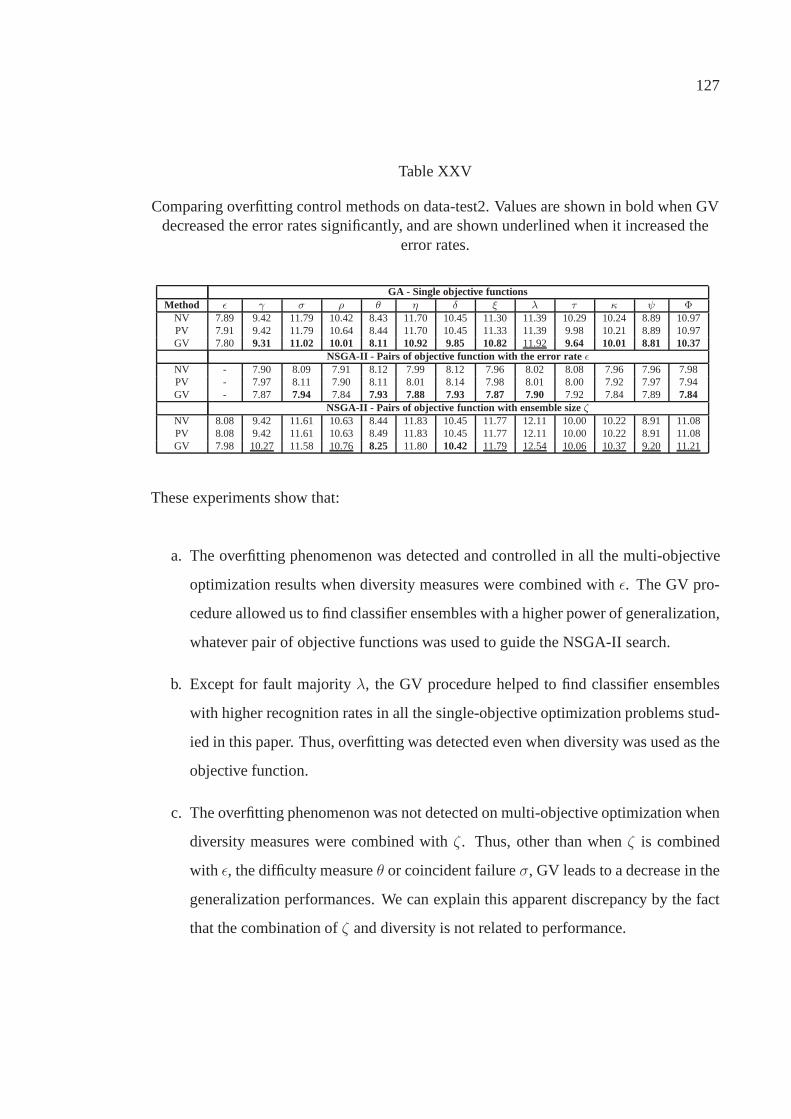
127

Table XXV

Comparing overfitting control methods on data-test2. Values are shown in bold when GVdecreased the error rates significantly, and are shown underlined when it increased the

error rates.

GA - Single objective functionsMethod ǫ γ σ ρ θ η δ ξ λ τ κ ψ Φ

NV 7.89 9.42 11.79 10.42 8.43 11.70 10.45 11.30 11.39 10.29 10.24 8.89 10.97PV 7.91 9.42 11.79 10.64 8.44 11.70 10.45 11.33 11.39 9.98 10.21 8.89 10.97GV 7.80 9.31 11.02 10.01 8.11 10.92 9.85 10.82 11.92 9.64 10.01 8.81 10.37

NSGA-II - Pairs of objective function with the error rate ǫNV - 7.90 8.09 7.91 8.12 7.99 8.12 7.96 8.02 8.08 7.96 7.96 7.98PV - 7.97 8.11 7.90 8.11 8.01 8.14 7.98 8.01 8.00 7.92 7.97 7.94GV - 7.87 7.94 7.84 7.93 7.88 7.93 7.87 7.90 7.92 7.84 7.89 7.84

NSGA-II - Pairs of objective function with ensemble sizeζNV 8.08 9.42 11.61 10.63 8.44 11.83 10.45 11.77 12.11 10.00 10.22 8.91 11.08PV 8.08 9.42 11.61 10.63 8.49 11.83 10.45 11.77 12.11 10.00 10.22 8.91 11.08GV 7.98 10.27 11.58 10.76 8.25 11.80 10.42 11.79 12.54 10.06 10.37 9.20 11.21

These experiments show that:

a. The overfitting phenomenon was detected and controlled inall the multi-objective

optimization results when diversity measures were combined with ǫ. The GV pro-

cedure allowed us to find classifier ensembles with a higher power of generalization,

whatever pair of objective functions was used to guide the NSGA-II search.

b. Except for fault majorityλ, the GV procedure helped to find classifier ensembles

with higher recognition rates in all the single-objective optimization problems stud-

ied in this paper. Thus, overfitting was detected even when diversity was used as the

objective function.

c. The overfitting phenomenon was not detected on multi-objective optimization when

diversity measures were combined withζ . Thus, other than whenζ is combined

with ǫ, the difficulty measureθ or coincident failureσ, GV leads to a decrease in the

generalization performances. We can explain this apparentdiscrepancy by the fact

that the combination ofζ and diversity is not related to performance.

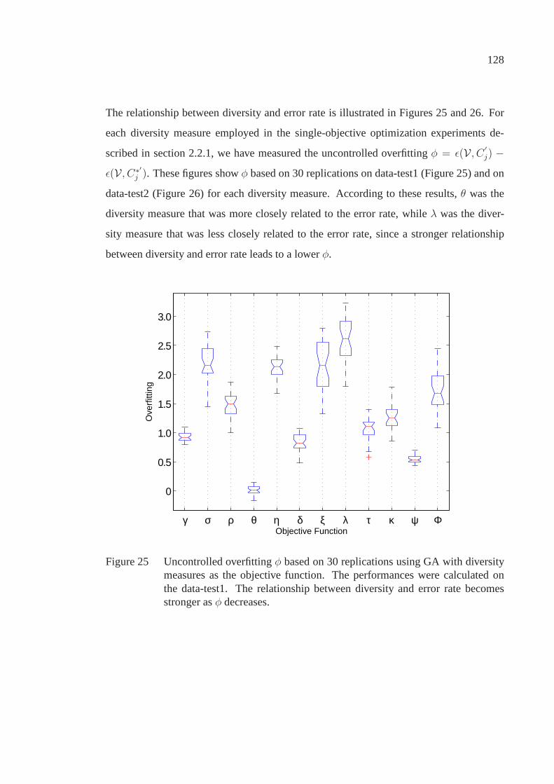
128

The relationship between diversity and error rate is illustrated in Figures 25 and 26. For

each diversity measure employed in the single-objective optimization experiments de-

scribed in section 2.2.1, we have measured the uncontrolledoverfittingφ = ǫ(V, C′

j) −

ǫ(V, C∗′j ). These figures showφ based on 30 replications on data-test1 (Figure 25) and on

data-test2 (Figure 26) for each diversity measure. According to these results,θ was the

diversity measure that was more closely related to the errorrate, whileλ was the diver-

sity measure that was less closely related to the error rate,since a stronger relationship

between diversity and error rate leads to a lowerφ.

γ σ ρ θ η δ ξ λ τ κ ψ Φ

0

0.5

1.0

1.5

2.0

2.5

3.0

Ove

rfitt

ing

Objective Function

Figure 25 Uncontrolled overfittingφ based on 30 replications using GA with diversitymeasures as the objective function. The performances were calculated onthe data-test1. The relationship between diversity and error rate becomesstronger asφ decreases.

129

γ σ ρ θ η δ ξ λ τ κ ψ Φ

0

0.5

1.0

1.5

2.0O

verf

ittin

g

Objective Function

Figure 26 Uncontrolled overfittingφ based on 30 replications using GA with diversitymeasures as the objective function. The performances were calculated onthe data-test2. The relationship between diversity and error rate becomesstronger asφ decreases.

However, the results related to the relationship between diversity measures and the error

rate may be different if the minimum number of classifiers is fixed and larger than we have

defined in this work, i.e. 5 classifiers. We investigate this aspect in chapter 3.

APPENDIX 3

Pareto Analysis

131

3.1 Introduction

Based on the results obtained in appendix 2 we observed that the performance of the so-

lutions found in both single- and multi-objective optimization processes was increased by

applying the global validation GV method to reduce overfitting. However, when ensemble

sizeζ and diversity were combined to make up pairs of objective functions to guide the

optimization and the validation processes, the results were very different. GV increased

the generalization error rates. We explained this behaviorin appendix 2 by the following

assumption: the combination ofζ and diversity is not related to the performance. First,

in despite of the fact that good results were obtained using GV guided by diversity in the

single-objective optimization approach, our experimentsoutlined that, although reduced,

overfitting was not totally controlled. Second, even if we can establish an analogy between

feature subset selection and SOCS, we cannot increase performance by selecting classifier

ensembles with the minimumζ , specially because we need to deal with a large initial pool

of classifiers. Therefore, we cannot decrease the generalization error rate by combining

this pair of objective functions.

In this appendix, we present further evidence on Pareto front analysis to show why diver-

sity andζ are not strongly related to the performance

3.2 Pareto Analysis

Objective functions in multi-objective optimization problems are often conflicting. Since

different tradeoffs are established over the Pareto front,when one solution is better ac-

cording to one objective, it is often worse according to the remaining objective functions.

Indeed, Deb [12] points out that, for instance in a two conflicting objective problem, if

a ranking of nondominated solutions is carried out in an ascending order according to

one objective function, a ranking in a descending order is obtained according to the other

objective function.

132

These observations are illustrated in Figure 27. NSGA-II was employed as the search

algorithm. In Figure 27(a) the search was guided by the minimization of the error rateǫ

and the difficulty measureθ. The Pareto front solutions are shown in an ascending order of

ǫ, consequently, in a descending order of theθ. Figure 27(b) shows the Pareto front found

using the following pair of objective functions: jointly minimizeǫ andζ . Once again, the

solutions were ordered according toǫ, and in a descending order ofζ . In Figure 27(c)

the pair of objective functions employed was the minimization of ζ andθ. The Pareto

solutions are shown in an ascending order ofθ (descending order ofζ). However, the

same behavior cannot be detected in Figure 27(d) where it is shown an example of the

evolution of the optimization process after 1,000 generations which was generated using

the following pair of objective functions: jointly minimize ζ and the interrater agreement

κ. It can be seen that only one solution was found over the Pareto front.

The first two figures show that eitherθ or ζ combined withǫ are conflicting objectives. In

Figure 27(c) it is shown thatθ andζ are also conflicting objectives. In contrast,κ andζ are

not conflicting objectives. In order to show whether or not the pairs of objective functions

applied in chapter 2 are conflicting objective functions we apply here two quality metrics

based on calculating the overall Pareto spread andkth objective Pareto spread introduced

by Wu and Azarm [103]. Given a multi-objective problem withm objective functions

f1, f2, . . . , fm, we show how to calculate the two measures of spread taking into account,

without loss of generality, all objective functions to be minimized and equally important.

Givensw be the possible worst solution andsb be the possible best solution, the objective

space should be scaled by the following equation:

fj(xk) =fj(xk) − f bjfwj − f bj

(3.1)

133

0.0359 0.036 0.036 0.0361 0.0361 0.0362 0.0362 0.03633.25

3.30

3.35

3.40

3.45

3.50

3.55

3.60

3.65

Difficulty

Err

or r

ate

(a)

4 6 8 10 12 14 16 183.2

3.4

3.6

3.8

4.0

4.2

4.4

4.6

4.8

5.0

Ensemble size

Err

or r

ate

(b)

4 6 8 10 12 14 16 18 20 220.035

0.036

0.037

0.038

0.039

0.040

0.041

0.042

Ensemble size

Diff

icul

ty

(c)

10 20 30 40 50 600.26

0.28

0.30

0.32

0.34

0.36

Ensemble size

Inte

rrat

erComplete search spaceNon−dominated solutions

(d)

Figure 27 Pareto front after 1000 generations found using NSGA-II and the pairs ofobjective functions: jointly minimize the error rate and the difficulty measure(a), jointly minimize the error rate and ensemble size (b), jointly minimizeensemble size and the difficulty measure (c) and jointly minimize ensemblesize and the interrater agreement (d).

In a two-objective problem, the scaled objective space is a hyper-rectangle, as shown in

Figure 28 defined by the scaled worst (1, 1) and best (0, 0) solutions. The overall Pareto

spread is defined as:

134

f 1

f 2

b

w

f 1min f, 2max( )

( f 1max, f2min )

s

s

Figure 28 Scaled objective space of a two-objective problemused to calculate theoverall Pareto spread and thekth objective Pareto spread.

OPS =

∏mi=1 |max

npk=1(pk)i −minnpk=1(pk)i|

∏mi=1 |(pw)i − (pb)i|

(3.2)

or

OPS =

m∏

i=1

|maxnpk=1[fi(xk)] −minnpk=1[fi(xk)] (3.3)

wherenp is the total number of Pareto solutions. When we are dealing with no conflicting

objective functionsOPS is equal to0. Hence, a wider spread leads to more diversity over

the Pareto front which is a desired Pareto property. However, OPS does not measure the

individual objective spread. For example, if instead of having 7 solutions over the Pareto

front as shown in Figure 28, we had only two solutions, for instance(f1min, f2max) and

(f1max, f2min), the sameOPS value would be obtained but the diversity over a Pareto with

only two solutions is much smaller than the diversity over a Pareto with 7 solutions. In

order to overcome this problem, thekth Objective Pareto Spread (IPS), also proposed by

Wu and Azarm[103], is applied. TheIPSk is calculated as:

135

IPSk =|maxnpi=1((pi)k) −minnpi=1((pi)k)|

|(pw)k − (pb)k|(3.4)

or

IPSk = |maxnpi=1(fk(xi)) −minnpi=1(fk(xi))| (3.5)

In the two-objective problem shown in Figure 28, thekth objective Pareto Spread and the

overall Pareto spread are respectively:

IPSf1 = |f1max − f1min| (3.6)

IPSf2 = |f2max − f2min| (3.7)

OPS = IPSf1IPSf2 (3.8)

The kth objective Pareto Spread is important to measure the diversity over the Pareto

front and to show whether or not spread is wider for one objective function than for the

others. We try to identify if there is more variation in one objective function or if the

objective functions are equally diverse. Table XXVI presents thekth objective Pareto

Spread and the overall Pareto spread calculated for each Pareto front shown in Figure 27.

136

The difficulty measureθ and the error rateǫ are conflicting objective functions but there

is much more variation amongǫ values than amongθ values. Ensemble sizeζ andǫ are

conflicting objective functions and there is more variationin ζ values than inǫ values. In

addition,θ andζ are conflicting objective functions but once again, there isless variation

amongθ values. It is important note that there is more variation among θ values when

this diversity measure is combined withζ than when it is combined withǫ. Finally, the

interrater agreementκ andζ are not conflicting objective functions.

Table XXVI

Worst and best points, minima and maxima points, thekth objective Pareto spread valuesand overall Pareto spread values for each Pareto front.

Objective Original values Scaled valuesFunctions sw sb min max sw sb min max IPS OPS

Difficulty θ (f1) 1 0 0.0359 0.0362 1 0 0.0359 0.0362 0.0003Error rateǫ (f2) 100 0 3.2800 3.5600 1 0 0.0328 0.0356 0.0028 0.1 x10−5

Ensemble sizeζ (f1) 100 0 5 17 1 0 0.0500 0.1700 0.1200Error rateǫ (f2) 100 0 3.2900 4.7000 1 0 0.0329 0.0470 0.0141 0.17 x10−2

Ensemble sizeζ (f1) 100 0 21 5 1 0 0.0500 0.2100 0.1600Difficulty θ (f2) 1 0 0.0415 0.0356 1 0 0.0356 0.0415 0.0059 0.9 x10−3

Ensemble sizeζ (f1) 100 0 5 5 1 0 0.0500 0.0500 0.0000Interraterκ (f2) 1 0 0.2752 0.2752 1 0 0.2752 0.2752 0.0000 0.0000

We have calculated both quality measures in order to show which measures are conflicting

or not. The same pairs of objective functions investigated in appendix 2 were used here:

diversity measures combined withǫ; diversity measures combined withζ andǫ combined

with ζ . Table XXVII shows the average results from 30 replicationsfor each pair of

objective functions. This table shows the values of thekth objective Pareto spread and the

overall Pareto spread, as well as the difference between thekth objective Pareto spreads.

This difference indicates the variation among objective functions values.

These results show that all diversity measures are conflicting objective functions when

combined withǫ. Except Kohavi-Wolpertψ, θ and ambiguityγ, there is more variation

among diversity values than amongǫ values. Ensemble sizeζ andǫ are also conflicting

137

objective functions and there is more variation amongζ values. However, there are only

three diversity measures which are conflicting objective functions when combined with

ensemble size, the sameψ, θ andγ.

Table XXVII

The averagekth objective Pareto spread values and the average overall Pareto spreadvalues for each pair of objective function.

Error rate Ensemble sizeDiversity IPSǫ IPSdiv IPSdiv − IPSǫ OPS IPSζ IPSdiv IPSζ − IPSdiv OPS

γ 0.0187 0.0254 0.0067 0.5 x10−3 0.0503 0.0030 -0.0474 0,0001σ 0.0134 0.0368 0.0234 0.5 x10−3 0.0000 0.0000 0.0000 0.0000ρ 0.0213 0.0442 0.0229 0.9 x10−3 0.0000 0.0000 0.0000 0.0000θ 0.0025 0.0006 -0.0019 0.2 x10−5 0.1733 0.0058 -0.1675 0.0010η 0.0330 0.0428 0.0098 0.14 x10−2 0.0000 0.0000 0.0000 0.0000δ 0.0159 0.0068 -0.0091 0.1 x10−3 0.0000 0.0000 0.0000 0.0000ξ 0.0249 0.0659 0.0410 0.17 x10−2 0.0000 0.0000 0.0000 0.0000λ 0.0192 0.0460 0.0268 0.9 x10−3 0.0000 0.0000 0.0000 0.0000τ 0.0150 0.0357 0.0207 0.5 x10−3 0.0000 0.0000 0.0000 0.0000κ 0.0159 0.0447 0.0288 0.7 x10−3 0.0000 0.0000 0.0000 0.0000ψ 0.0119 0.0113 -0.0006 0.1 x10−3 0.1000 0.0079 -0.0921 0.0008Φ 0.0265 0.0927 0.0662 0.25 x10−2 0.0000 0.0000 0.0000 0.0000

Ensemble sizeζ and Error rate ǫIPSǫ IPSζ IPSζ − IPSǫ OPS0.0119 0.2163 0.2045 0.0025

The literature has shown that the pairwise diversity measures andζ are not conflicting

objective functions. Aksela and Laaksonen [1] observe thatpairwise diversity measures

always try to find the two most diverse classifiers which leadsto the minimization of the

number of classifiers during the optimization process. Our results confirm this observation

since all pairwise measures (see Chapter 2, section 2.2.1 employed in our experiments are

not conflicting objective functions when combined withζ . However, our results show

that some of the nonpairwise measures lead also to the minimization ofζ . Three of the

nonpairwise measures employed:γ, θ andψ, do not minimizeζ .

According to Whitaker and Kuncheva [99] nonpairwise measures are calculated by using

either entropy or correlation between individual outputs and the ensemble’s output or dis-

tribution of “difficulty” of the data samples. Among the three diversity measures, which

138

are conflicting objective functions when combined withζ , two measures are based on

the variance over the dataset (θ andψ) andγ is based on the variance among ensemble’s

members. Thus, our observation is that, besides the pairwise diversity measures pointed

out by Aksela and Laaksonen [1], all non-pairwise diversitymeasures based on entropy or

correlation between individual outputs are also not able tofind the best ensemble’s size,

i.e. they minimizeζ during the optimization process.

Moreover, there is no guarantee of finding the best ensemble’s size using one of the three

diversity measures based on variance, specially ambiguity, which generates the less diverse

Pareto front (Table XXVII and Figure 29(a)) and the smallestclassifier ensembles (Figure

29(a)). However, these three measures have such a property that makes them able to

generate larger classifier ensembles, which is useful in OCSmethods since we deal with

a large initial pool of classifiers. The two diversity measures based on the variance over

the dataset found more diverse Pareto front and larger classifier ensembles than ambiguity

(based on the variance of the classifiers’ output). The difficulty measureθ was better than

Kohavi-Wolpertψ in these two aspects, as it can seen in Figure 29(b) forψ and in Figure

27(c) forθ, as well as in Table XXVII.

139

5 6 7 8 9 10 110.139

0.14

0.141

0.142

0.143

0.144

0.145

0.146

Ensemble Size

Am

bigu

ity

(a)

4 6 8 10 12 14 16 180.137

0.138

0.139

0.14

0.141

0.142

0.143

0.144

0.145

0.146

Ensemble Size

Koh

avi−

Wol

pert

(b)

Figure 29 Pareto front after 1000 generations found using NSGA-II and the pairs ofobjective functions: minimize ensemble size and maximize ambiguity (a)and minimize ensemble size and maximize Kohavi-Wolpert (b).

APPENDIX 4

Illustration of overfitting in single- and multi-objective GA

141

In this appendix we show the Figures 13 and 13, which illustrated the overfitting problem

in single- and multi-objective GA in chapter 3, in larger versions.

20 30 40 50 60 70 80 90 1003.0

3.2

3.4

3.6

3.8

4.0

4.2

4.4

4.6

4.8

5.0

Ensemble size

Err

or r

ate

Cj (evaluated)

Cj*(1)

(a) O dataset andg = 1

20 30 40 50 60 70 80 90 1003.0

3.2

3.4

3.6

3.8

4.0

4.2

4.4

4.6

4.8

5.0

Ensemble size

Err

or r

ate

Cj (to evaluate)

Cj (evaluated)

Cj*(1)

(b) V dataset andg = 1

Figure 30 Optimization using GA guided byǫ. Here, we follow the evolution ofC∗j (g)

(diamonds) forg = 1 (Figure 30(a)) on the optimization datasetO, as wellas on the validation datasetV (Figure 30(b)). Solutions not yet evaluated arein grey and the best performing solutions are highlighted byarrows.

142

20 30 40 50 60 70 80 90 1003.0

3.2

3.4

3.6

3.8

4.0

4.2

4.4

4.6

4.8

5.0

Ensemble size

Err

or r

ate

Cj (to evaluate)

Cj (evaluated)

Cj*(52)

(a) O dataset andg = 52

20 30 40 50 60 70 80 90 1003.0

3.2

3.4

3.6

3.8

4.0

4.2

4.4

4.6

4.8

5.0

Ensemble size

Err

or r

ate

Cj (to evaluate)

Cj (evaluated)

Cj*(52)

(b) V dataset andg = 52

Figure 31 Optimization using GA guided byǫ. Here, we follow the evolution ofC∗j (g)

(diamonds) forg = 52 (Figure 31(a)) on the optimization datasetO, as wellas on the validation datasetV (Figure 31(b)). The minimal error is reachedslightly afterg = 52 onV, and overfitting is measured by comparing it to theminimal error reached onO. Solutions not yet evaluated are in grey and thebest performing solutions are highlighted by arrows.

20 30 40 50 60 70 80 90 1003.0

3.2

3.4

3.6

3.8

4.0

4.2

4.4

4.6

4.8

5.0

Ensemble size

Err

or r

ate

Cj

Cj*

Cj*’

(a) O dataset andmax(g)

20 30 40 50 60 70 80 90 1003.0

3.2

3.4

3.6

3.8

4.0

4.2

4.4

4.6

4.8

5.0

Ensemble size

Err

or r

ate

Cj

Cj*

Cj*’

overfitting

(b) V dataset andmax(g)

Figure 32 Optimization using GA guided byǫ. Here, we follow the evolution ofC∗j (g)

(diamonds) formax(g) (Figure 32(a)) on the optimization datasetO, as wellas on the validation datasetV (Figure 32(b)). The overfitting is measured asthe difference in error betweenC∗′

j (circles) andC∗j (32(b)). There is a 0.30%

overfit in this example. Solutions not yet evaluated are in grey and the bestperforming solutions are highlighted by arrows.

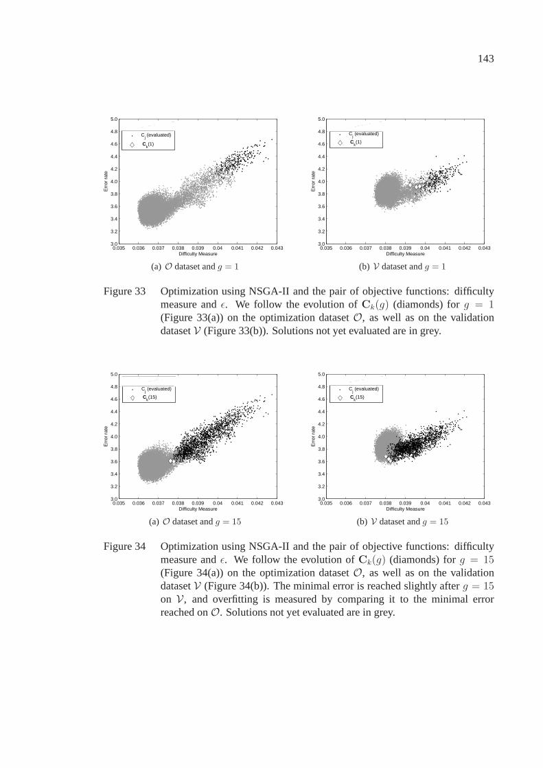
143

0.035 0.036 0.037 0.038 0.039 0.04 0.041 0.042 0.0433.0

3.2

3.4

3.6

3.8

4.0

4.2

4.4

4.6

4.8

5.0

Difficulty Measure

Err

or r

ate

Cj (to evaluate)

Cj (evaluated)

Ck(1)

(a) O dataset andg = 1

0.035 0.036 0.037 0.038 0.039 0.04 0.041 0.042 0.0433.0

3.2

3.4

3.6

3.8

4.0

4.2

4.4

4.6

4.8

5.0

Difficulty Measure

Err

or r

ate

Cj (to evaluate)

Cj (evaluated)

Ck(1)

(b) V dataset andg = 1

Figure 33 Optimization using NSGA-II and the pair of objective functions: difficultymeasure andǫ. We follow the evolution ofCk(g) (diamonds) forg = 1(Figure 33(a)) on the optimization datasetO, as well as on the validationdatasetV (Figure 33(b)). Solutions not yet evaluated are in grey.

0.035 0.036 0.037 0.038 0.039 0.04 0.041 0.042 0.0433.0

3.2

3.4

3.6

3.8

4.0

4.2

4.4

4.6

4.8

5.0

Difficulty Measure

Err

or r

ate

Cj (to evaluate)

Cj (evaluated)

Ck(15)

(a) O dataset andg = 15

0.035 0.036 0.037 0.038 0.039 0.04 0.041 0.042 0.0433.0

3.2

3.4

3.6

3.8

4.0

4.2

4.4

4.6

4.8

5.0

Difficulty Measure

Err

or r

ate

Cj (to evaluate)

Cj (evaluated)

Ck(15)

(b) V dataset andg = 15

Figure 34 Optimization using NSGA-II and the pair of objective functions: difficultymeasure andǫ. We follow the evolution ofCk(g) (diamonds) forg = 15(Figure 34(a)) on the optimization datasetO, as well as on the validationdatasetV (Figure 34(b)). The minimal error is reached slightly afterg = 15on V, and overfitting is measured by comparing it to the minimal errorreached onO. Solutions not yet evaluated are in grey.

144

0.035 0.036 0.037 0.038 0.039 0.04 0.041 0.042 0.0433.0

3.2

3.4

3.6

3.8

4.0

4.2

4.4

4.6

4.8

5.0

Difficulty Measure

Err

or r

ate

Cj

Ck*

Ck*’

(a) O dataset andmax(g)

0.035 0.036 0.037 0.038 0.039 0.04 0.041 0.042 0.0433.0

3.2

3.4

3.6

3.8

4.0

4.2

4.4

4.6

4.8

5.0

Difficulty Measure

Err

or r

ate

Cj

Ck*

Ck*’

overfitting

(b) V dataset andmax(g)

Figure 35 Optimization using NSGA-II and the pair of objective functions: difficultymeasure andǫ. We follow the evolution ofCk(g) (diamonds) formax(g)(Figure 35(a)) on the optimization datasetO, as well as on the validationdatasetV (Figure 35(b)). The overfitting is measured as the difference inerror between the most accurate solution inC

∗′

k (circles) and inC∗k (35(b)).

There is a 0.20% overfit in this example. Solutions not yet evaluated are ingrey.

APPENDIX 5

Comparison between Particle Swarm Optimization and Genetic Algorithm taking

into account overfitting

146

The objective of this appendix is to present the results of a short comparative study be-

tween Particle Swarm Optimization (PSO) [34] and GA in orderto show which algorithm

is more prone to overfitting. These experiments were conducted using only the error rate

ǫ as the objective function. The comparative study is focusedon detecting and controlling

overfitting in both GA and PSO search algorithms at the optimization process, by applying

the global validation strategy GV.

5.1 Particle Swarm Optimization

PSO simulates the behaviors of bird flocking or fish schooling. Each individual of the pop-

ulation is called particles. All particles have fitness values which are evaluated during the

optimization process of the selection phase of SOCS. Algorithm 8 summarizes the variant

of the PSO algorithm used in this appendix. This variant is called global neighborhood

[57] in the literature.

Algorithm 8 PSO1: for each particledo2: Initialize particle3: end for4: while maximum iterations or stop criteria are not attaineddo5: for each particledo6: Compute fitness value7: if fitness value is better than the best fitness (pBest) in historythen8: Set current value as the newpBest9: end if

10: end for11: Choose the particle with the best fitness as thegBest12: for each particledo13: Compute its velocity14: Update its position15: end for16: end while

147

The solutiongBest denotes the best particle in the whole population. In PSO thepopu-

lation is called swarm. LettingC(g) denote the swarm in iterationg andǫ represent the

objective function, the complete GV algorithm for PSO is described in Algorithm 9.

Algorithm 9 Global Validation for PSO1: Creates initial swarm2: A = ∅3: Validate all solutions inC(1) over samples contained inV4: FindC∗′

j (1) from C(1)

5: SetC∗′

j :=C∗′

j (1)6: for each iterationg ∈ 1, . . . , max(g) do7: run PSO and generateC(g + 1)8: validate all solutions inC(g + 1)9: findC∗′

j (g + 1)

10: if ǫ(V, C∗′j )(g + 1) < ǫ(V, C∗′

j ) then11: setC∗′

j := C∗′j (g + 1)

12: updateA by storing in it the newC∗′j

13: end if14: end for15: return C∗′

j stored inA

5.2 Experiments

In order to develop our experiments we use the two large datasets described in chapter

3, Table VI: NIST-digits and NIST-letters. The same initialpool of 100 kNN classifiers

generated by applying the Random Subspace method is investigated here.

Table XXVIII shows the average results from 30 replicationsobtained using NIST-digits

dataset. Values are shown in bold when GV decreased the generalization error signif-

icantly, according to the Kruskal-Wallis statistical test. The results with no overfitting

control NV are also included in this table. These initial results show that although both

search algorithms are prone to overfitting, GA appears to be more affected. It is important

to note that this behavior confirms Reunamen’s work [65]. He pointed out that the degree

of overfitting increases as the intensity of search increases. Figure 36(a) shows that GA

148

needs more generations to find the best solution during the optimization process than PSO.

On the other hand, the best solutionC∗′

j stored inA is found much earlier using GA than

PSO (Figure 36(b)). This result can be explained by the fact that, since during the opti-

mization process PSO keeps searching by solutions even worse thangBest, it is possible

to generate solutions that are better in generalization after findinggBest.

Table XXVIII

Comparing GA and PSO in terms of overfitting control on NIST-digits dataset. Valuesare shown in bold when GV decreased the error rates significantly. The results were

calculated using data-test1 and data-test2.

Validation Method GA PSOdata-test1 data-test2 data-test1 data-test2

NV 3.60 7.91 3.62 8.02GV 3.55 7.80 3.61 7.88

GA PSO

100

200

300

400

500

600

700

Gen

erat

ion

of B

est S

olut

ion

Search Algorithm

(a)

GA PSO

0

100

200

300

400

500

600

700

800

900

Gen

erat

ion

of B

est S

olut

ion

Search Algorithm

(b)

Figure 36 NIST-digits: the convergence points of GA and PSO.The generation whenthe best solution was found on optimization (36(a)) and on validation (36(b)).

However, the experiments with NIST-letters did not confirm our first observations. The

average results from 30 replications obtained using NIST-letters dataset are reported in

Table XXIX. These results show that GV only slightly decreased the generalization error

149

rate for NIST-letters. In despite of this, the results obtained using NIST-letters dataset

allow us to confirm that GA performs a more intense search process. Figure 37(a) shows

that GA needs more generations to find the best solution during the optimization process

than PSO also on NIST-letters dataset. Again, GA findsC∗′j much earlier than PSO (Figure

37(b)). Moreover, the performance of the solutions found byGA were slightly better

using both NIST-digits (Figure 38) and NIST-letters (Figure 39(a)) datasets. However,

the classifier ensembles found employing GA were larger thanthose found using PSO, as

illustrated in Figure 40 for NIST-digits and in Figure 39(b)for NIST-letters.

Table XXIX

Comparing GA and PSO in terms of overfitting control on NIST-letter dataset.

Data set No validation Global validationGA PSO GA PSO

NIST-letters 6.49 6.54 6.44 6.49

GA PSO

100

200

300

400

500

600

700

800

900

Gen

erat

ion

of B

est S

olut

ion

Search Algorithm

(a)

GA PSO

0

100

200

300

400

500

600

700

800

900

1000

Gen

erat

ion

of B

est S

olut

ion

Search Algorithm

(b)

Figure 37 NIST-letters: the convergence points of GA and PSO. The generation whenthe best solution was found on optimization (37(a)) and on validation (37(b)).

150

GA PSO

3.45

3.50

3.55

3.60

3.65

3.70

3.75

Err

or r

ate

Search Algorithm

(a)

GA PSO

7.6

7.7

7.8

7.9

8.0

8.1

8.2

Err

or r

ate

Search Algorithm

(b)

Figure 38 NIST-digits: error rates of the solutions found on30 replications using GAand PSO. The performances were calculated on the data-test1(38(a)) and onthe data-test2 (38(b)).

GA PSO6.2

6.3

6.4

6.5

6.6

6.7

6.8

6.9

7

7.1

Err

or r

ate

Search Algorithm

(a)

GA PSO

30

40

50

60

70

80

90

Ens

embl

e S

ize

Search Algorithm

(b)

Figure 39 NIST-letters: error rates of the solutions found on 30 replications using GAand PSO (39(a)). Size of the ensembles found using both GA andPSO searchalgorithms (39(b)).

151

GA PSO25

30

35

40

45

50

Ens

embl

e S

ize

Search Algorithm

Figure 40 NIST-digits: Size of the ensembles found using both GA and PSO searchalgorithms.

BIBLIOGRAPHY

[1] M. Aksela and J. Laaksonen. Using diversity of errors forselecting members of acommittee classifier.Pattern Recognition, 39(4):608–623, 2006.

[2] H. Altinçay. Ensembling evidential k-nearest neighborclassifiers through multi-modal pertubation.Applied Soft Computing, 7(3):1072–1083, 2007.

[3] S. Bandyopadhyay, S.K. Pal, and B. Aruna. Multiobjective gas, quantitative indices,and pattern classification.IEEE Transactions on System, Man, and Cybernetics -PartB, 34(5):2088–2099, 2004.

[4] N. Benahmed. Optimisation de réseaux de neurones pour lareconnaissance dechiffres manuscrits isolés: Sélection et pondération des primitives par algorithmesgénétiques. Master’s thesis, École de technologie supérieure, 2002.

[5] L. Breiman. Bagging predictors.Machine Learning, 24(2):123–140, 1996.

[6] L. Breiman. Randomizing outputs to increase predictionaccuracy. MachineLearning, 40(3):229–242, 2000.

[7] G. Brown, J. Wyatt, R. Harris, and X. Yao. Diversity creation methods: a surveyand categorisation.Information Fusion, 6(1):5–20, 2005.

[8] A. Canuto, G. Howells, and M. Fairhurst. The use of confidence measures toenhance combination strategies in multi-network neuro-fuzzy systems.ConnectionScience, 12(3/4):315–331, 2000.

[9] A. Canuto, M.C.C.Abreu, L.M. Oliveira, J.C. Xavier Jr.,and A. M. Santos.Investigating the influence of the choice of the ensemble members in accuracyand diversity of selection-based and fusion-based methodsfor ensembles.PatternRecognition Letters, 28:472–486, 2007.

[10] D. Corne and J. Knowles. No free lunch and free leftoverstheorems formultiobjective optimization problems. InProceedings of Evolutionary Multi-Criterion Optimization, pages 327–341, Faro, Portugal, 2003.

[11] K. Deb. Multi-Objective Optimization using Evolutionary Algorithms. John Wiley& Sons, LTD, 2001.

[12] K. Deb. Unveiling innovative design principles by means of multiple conflictingobjectives.Engineering Optimization, 35(5):445–470, 2003.

153

[13] K. Deb, S. Agrawal, A. Pratab, and T. Meyarivan. A fast elitist non-dominatedsorting genetic algorithm for multi-objective optimization: Nsga-ii. InProceedingsof the Parallel Problem Solving from Nature VI Conference, pages 849–858, Paris,France, 2000.

[14] K. Deb and T. Goel. Controlled elitist non-dominated sorting genetic algorithmsfor better convergence. InProceedings of First Evolutionary Multi-CriterionOptimization, pages 67–81, 2001.

[15] L. Didaci, G. Giacinto, F. Roli, and G.L. Marcialis. A study on the performancesof the dynamic classifier selection based on local accuracy estimation. PatternRecognition, 28:2188–2191, 2005.

[16] T. G. Dietterich. Ensemble methods in machine learning. In Proceedings of IInternational Workshop on Multiple Classifier System, pages 1–15, Cagliari, Italy,2000.

[17] T.G. Dietterich. An experimental comparison of three methods for constructingensembles of decision trees: Bagging, boosting, and randomization. MachineLearning, 40(2):139–158, 2000.

[18] T.G. Dietterich and G. Bakiri. Solving multiclass learning problems via error-correting output codes.Journal of Artificial Intteligence Research, 2:263–286,1995.

[19] P. Domingos. A unified bias-variance decomposition andits applications. InProc.17th International Conf. on Machine Learning, pages 231–238. Morgan Kaufmann,San Francisco, CA, 2000.

[20] J. Franke and M. Oberlander. Writing style detection bystatistical combinationof classifiers in form reader applications. InProceedings of II InternationalConference on Document Analysis and Recognition, pages 581–584, 1993.

[21] Y. Freund and R. Schapire. Experiments with a new boosting algorithm. InProceedings of XIII International Conference on Machine Learning, pages 148–156, 1996.

[22] H. Frohlich and O. Champelle. Feature selection for support vector machines bymeans of genetic algorithms. InProceedings of IEEE International Conference onTools with AI, pages 142–148, 2003.

[23] B. Gabrys and D. Ruta. Genetic algorithms in classifier fusion. Applied SoftComputing, 6(4):337–347, 2006.

154

[24] G. Giacinto and F. Roli. Dynamic classifier selection based on multiple classifierbehaviour.Pattern Recognition, 33:1879–1881, 2001.

[25] P.J. Gother. NIST Special Database 19 - Handprited forms and charactersdatabase. National Institute of Standard and Technology - NIST : database CDdocumentation, 1995.

[26] D. Greene, A. Tsymbal, N. Bolshakova, and P. Cunningham. Ensemble clusteringin medical diagnostics. InProceedings of the IEEE Symposium on Computer-BasedMedical Systems, pages 570–575, Bethesda, USA, 2004.

[27] A.J. Grove and D. Schuurmans. Boosting in the limit: Maximizing the marginof learned ensembles. InProceedings of 15th National Conference on ArtificialIntelligence, pages 692–699, 1998.

[28] V. Gunes, M. Menard, and P. Loonis. A multiple classifiersystem usingambiguity rejection for clustering-classification cooperation. International Journalof Uncertainty, Fuzziness and Knowledge-Based Systems, 8(6):747–762, 2000.

[29] L.K. Hansen, C. Liisberg, and P. Salomon. The error-reject tradeoff.Open Systems& Information Dynamics, 4(2):159–184, 1997.

[30] T. K. Ho. Multiple classifier combination: Lessons and next steps. In A. Kandel andH. Bunke, editors,Hybrid Methods in Pattern Recognition, pages 171–198. WorldScientific, 2002.

[31] T.K. Ho. Nearest neighbors in random subspaces. InProceedings of the SecondInternational Workshop on Statistical Techniques in Pattern Recognition, pages640–648, Sydney, Australia, 1998.

[32] T.K. Ho. The random subspace method for constructing decision forests. IEEETransactions on Pattern Analysis and Machine Intelligence, 20(8):832–844, 1998.

[33] Y.S. Huang and C. Suen. Combination of multiple expertsfor the recognition ofunconstrained handwritten numerals.IEEE Transactions on Pattern Analysis andMachine Intelligence, 17(1):90–94, 1995.

[34] J. Kennedy and R.C. Eberhart. Particle swarm intelligence. In Proceedings ofInternational Conference on Neural Network, pages 1942–1948, 1995.

[35] J. Kittler, M. Hatef, RPW. Duin, and J. Matas. On combining classifiers.IEEETransactions on Pattern Analysis and Machine Intelligence, 20(3):226–238, 1998.

155

[36] A. Ko, R. Sabourin, and A. Britto Jr. A new dynamic ensemble selection method fornumeral recognition. InProceedings of the 7th International Workshop on MultipleClassifier Systems, Prague-Czech Republic, 2007.

[37] R. Kohavi and D. Sommerfield. Feature subset selection using the wrapper model:Overfitting and dynamic search space topology. InProceedings of The FirstInternational Conference on Knowledge Discovery and Data Mining, pages 192–197, 1995.

[38] L.I. Kuncheva. Cluster-and-selection model for classifier combination. InProceedings of International Conference on Knowledge Based IntelligentEngineering Systems and Allied Technologies, pages 185–188, 2000.

[39] L.I. Kuncheva. Switching between selection and fusionin combining classifiers:An experiment.IEEE Transactions on Systems, Man, and Cybernetics, 32(2):146–156, 2002.

[40] L.I. Kuncheva. Combining Pattern Classifiers: Methods and Algorithms. JhonWiley & Sons, LTD, USA, 2004.

[41] L.I. Kuncheva, J. Bezdek, and R. Duin. Decision templates for multiple classifierfusion: an experimental comparison.Pattern Recognition, 34(2):299–314, 2001.

[42] L.I. Kuncheva, M.Skurichina, and R.P.W. Duin. An experimental study on diversityfor bagging and boosting with linear classifiers.Information Fusion, 3(4):245–258,2002.

[43] L.I. Kuncheva and J. Rodriguez. Classifier ensembles with a random linear oracle.IEEE Transactions on Knowledge and Data Engineering, 19(4):500–508, 2007.

[44] L.I. Kuncheva and C.J. Whitaker. Measures of diversityin classifier ensemblesan their relationship with the ensemble accuracy.Machine Learning, 51:181–207,2002.

[45] R. Liu and B. Yuan. Multiple classifiers combination by clustering and selection.Information Fusion, 2(4):163–168, 2001.

[46] X. Llorà, D.E. Goldberg, I. Traus, and E. Bernadó i Mansilla. Accuracy, parsimony,and generality in evolutionary learning systems via multiobjective selection. InInternational Workshop in Learning Classifier Systems, pages 118–142, 2002.

[47] J. Loughrey and P. Cunningham. Overfitting in wrapper-based feature subsetselection: The harder you try the worse it gets. InProceedings of InternationalConference on Innovative Techniques and Applications of AI, pages 33–43, 2004.

156

[48] D.D. Margineantu and T.G. Dietterich. Pruning adaptive boosting. InProceedingsof the International Conference on Machine Learning, pages 358–366, 1997.

[49] T. M. Mitchell. Machine Learning. McGraw-Hill, USA, 1997.

[50] N. Narasimhamurthy. Evaluation of diversity measuresfor binary classifierensembles. InProceedings of MCS, pages 267–277, Seaside, USA, 2005.

[51] L.S. Oliveira, M. Morita, R. Sabourin, and F. Bortolozi. Multi-objective geneticalgorithms to create ensemble of classifiers. InProceedings of the InternationalConference on Evolutionary Multi-Criterion Optimization, pages 592–606, 2005.

[52] L.S. Oliveira, R. Sabourin, F. Bortolozzi, and C.Y. Suen. Automatic recognitionof handwritten numerical strings: A recognition and verification strategy. IEEETransactions on Pattern Analysis and Machine Intelligence, 24(11):1438–1454,2002.

[53] D. W. Opitz and J. W. Shavlik. Actively searching for an effective neural-networkensemble.Connection Science, 8(3/4):337–353, 1996.

[54] N.C. Oza and K. Tumer. Classifier ensembles: select real-world applications.Information Fusion, 9(1):4–20, 2008.

[55] D. Parikh and R. Polikar. An ensemble-based incremental learning approach to datafusion. IEEE Transactions on Systems, Man, and Cybernetics-PartB, 37(2):500–508, 2007.

[56] Y. Park and J. Sklansky. Automated design of linear treeclassifiers. PatternRecognition, 23(12):1393–1412, 1990.

[57] K.E. Parsopoulos and M.N. Vrahatis. Recent approachesto global optimizationproblems through particle swarm optimization.Natural Computing, 1(2):235–306,2002.

[58] D. Partridge and W.B. Yates. Engineering multiversionneural-net systems.NeuralComputation, 8(4):869–893, 1996.

[59] M. Prior and T. Windeatt. Over-fitting in ensembles of neural networks classifierswithin ecoc frameworks. InProceedings of International Workshop on MultipleClassifier System, pages 286–295, Seaside, USA, 2005.

[60] J.R. Quinlan.Programs for Machine Learning. Morgan Kaufmann, 1993.

157

[61] P.V.W. Radtke. Classification Systems Optimization with Multi-ObjectiveEvolutionary Algorithms. PhD thesis, Ecole de Technologie Superieure - Universitedu Quebec, 2006.

[62] P.V.W. Radtke, R. Sabourin, and T. Wong. Impact of solution over-fit onevolutionary multi-objective optimization for classification systems. InProceedingsof IJCNN, Vancouver, Canada - accepted, 2006.

[63] G. Ratsch, T. Onoda, and K-R. Muller. An improvement of adaboost to avoidoverfitting. In Proceedings of The Fifth International Conference on NeuralInformation Processing, pages 506–509, Kitakyushu, Japan, 1998.

[64] R. Reed. Pruning algorithms - a survey.IEEE Transactions on Neural Networks,4(5):740–747, 1993.

[65] J. Reunanen. Overfitting in making comparisons betweenvariable selectionmethods.Journal of Machine Learning Research, 3:1371–1382, 2003.

[66] F. Rheaume, A-L. Jousselme, D. Grenier, E. Bosse, and P.ValinThomas. Newinitial basic probability assignments for multiple classifiers. InProceedings of XISignal Processing, Sensor Fusion, and Target Recognition, pages 319–328, 2002.

[67] D. Robilliard and C. Fonlupt. Backwarding: An overfitting control for geneticprogramming in a remote sensing application. InProceedings of the 5th EuropeanConference on Artificial Evolution, pages 245–254, 2000.

[68] G. Rogova. Combining the results of several neural network classifiers. NeuralNetworks, 7(5):777–781, 1994.

[69] F. Roli, G. Giacinto, and G. Vernazza. Methods for designing multiple classifiersystems. InProceedings of the International Workshop on Multiple ClassifierSystem, pages 78–87, 2001.

[70] D. Ruta and B. Gabrys. Classifier selection for majorityvoting. Information Fusion,6(1):163–168, 2005.

[71] D. Ruta and B. Gabrys. Neural network ensembles for timeseries prediction. InProceedings of the IEEE International Joint Conference on Neural Network, pages1204–1209, Orlando, USA, 2007.

[72] E.M. Dos Santos, R. Sabourin, and P. Maupin. Single and multi-objectivegenetic algorithms for the selection of ensemble of classifiers. InProceedings ofInternational Joint Conference on Neural Networks, pages 5377–5384, 2006.

158

[73] E.M. Dos Santos, R. Sabourin, and P. Maupin. Ambiguity-guided dynamicselection of ensemble of classifiers. InProceedings of International Conferenceon Information Fusion, Quebec, CA, 2007.

[74] E.M. Dos Santos, R. Sabourin, and P. Maupin. A dynamic overproduce-and-choosestrategy for the selection of classifier ensembles.Submitted to Pattern Recognition,2007.

[75] E.M. Dos Santos, R. Sabourin, and P. Maupin. Overfittingcautious selection ofclassifier ensembles with genetic algorithm.Submitted to Information Fusion, 2007.

[76] S.B. Serpico, L. Bruzzone, and F. Roli. An experimentalcomparison of neural andstatistical non-parametric algorithms for supervised classification of remote-sensingimages.Pattern Recognition Letters, 17(13):1331–1341, 1996.

[77] A.J.C. Sharkey. Multi-net systems. InCombining Artificial Neural Nets: Ensembleand Modular Multi-Net Systems, pages 1–27. Spring-Verlag, 1999.

[78] A.J.C. Sharkey and N.E Sharkey. The "test and select" approach to ensemblecombination. In J. Kittler and F. Roli, editors,Multiple Classifier System, pages30–44. Spring-Verlag, 2000.

[79] H.W. Shin and S.Y. Sohn. Combining both ensemble and dynamic classifierselection schemes for prediction of mobile internet subscribers. Expert Systemswith Applications, 25:63–68, 2003.

[80] H.W. Shin and S.Y. Sohn. Selected tree classifier combination based on bothaccuracy and error diversity.Pattern Recognition, 38(2):191–197, 2005.

[81] S. Singh and M. Singh. A dynamic classifier selection andcombination approachto image region labelling.Signal Processing: Image Communication, 20:219–231,2005.

[82] K. Sirlantzis, M.C. Fairhurst, and R.M. Guest. An evolutionary algorithmfor classifier and combination rule selection in multiple classifier system. InProceedings of ICPR, pages 771–774, 2002.

[83] P. C. Smits. Multiple classifier systems for supervisedremote sensing imageclassification based on dynamic classifier selection.IEEE Transactions onGeoscience and Remote Sensing, 40(4):801–813, 2002.

[84] R.G.F. Soares, A. Santana, A.M.P. Canuto, and M.C.P. deSouto. Using accuracyand diversity to select classifiers to build ensembles. InProceedings of InternationalJoint Conference on Neural Networks, pages 2289–2295, 2006.

159

[85] S.Y. Sohn and H.W. Shin. Experimental study for the comparison of classifiercombination methods.Pattern Recognition, 40(1):33–40, 2007.

[86] C.Y. Suen and Louisa Lam. Multiple classifier combination methodologies fordifferent output levels. InFirst International Workshop on Multiple ClassifierSystems, pages 52–66, London, UK, 2000.

[87] T. Suttorp and C. Igel. Multi-objective optimization of support vector machines.Studies in Computational Intelligence - Multi-objective Machine Learning, 16:199–220, 2006.

[88] G. Tremblay. Optimisation d’ensembles de classifieursnon paramétriques avecaprentissage par représentation partielle de l’information. Master’s thesis, École detechnologie supérieure, 2004.

[89] G. Tremblay, R. Sabourin, and P. Maupin. Optimizing nearest neighbour inrandom subspaces using a multi-objective genetic algorithm. In Proceedings ofInternational Conference Pattern Recognition, pages 208–211, Cambridge, UK,2004.

[90] A. Tsymbal, M. Pechenizkiy, and P. Cunningham. Diversity in search strategies forensemble feature selection.Information Fusion, 6(1):83–98, 2005.

[91] A. Tsymbal, M. Pechenizkiy, and P. Cunningham. Sequential genetic search forensemble feature selection. InProceedings of International Joint Conference onArtificial Intelligence, pages 877–882, 2005.

[92] A. Tsymbal, M. Pechenizkiy, P. Cunningham, and S. Puuronen. Dynamicintegration of classifiers for handling concept drift.Information Fusion, 9(1):56–68, 2008.

[93] G. Valentini. Ensemble methods based on bias-variance analysis. PhD thesis,Genova University, 2003.

[94] G. Valentini and T. Dietterich. Low bias bagged supportvector machines. InProc.International Conf. on Machine Learning, pages 776–783, 2003.

[95] G. Valentini and T. G. Dietterich. Bias-variance analysis and ensembles of svm. InF. Roli and J. Kittler, editors,Multiple Classifier System, pages 222–231. Spring-Verlag, 2002.

[96] X. Wang and H. Wang. Classification by evolutionary ensembles. PatternRecognition, 39(4):595–607, 2006.

160

[97] C. Wenzel, S. Baumann, and T. Jager. Advances in document classification byvoting of competitive approaches. In J.J. Hull and S. Lebowitz, editors,DocumentAnalysis Systems II, pages 385–405. World Scientific, 1998.

[98] K-D. Wernecke. A coupling procedure for the discrimination of mixed data.Biometrics, 48(2):497–506, 1992.

[99] C.J. Whitaker and L.I. Kuncheva. Examining the relationship between majorityvote accuracy and diversity in bagging and boosting. Technical report, School ofInformatics, Unversity of Wales, 2003.

[100] S. Wiegand, C. Igel, and U. Handmann. Evolutionary multi-objective optimizationof neural networks for face detection.International Journal of ComputationalIntelligence and Applications, 4(3):237–253, 2004.

[101] K. Woods. Combination of multiple classifiers using local accuracy estimates.IEEETransactions on Pattern Analysis and Machine Intelligence, 19(4):405–410, 1997.

[102] H. Wu and J.L. Shapiro. Does overfitting affect performance in estimationof distribution algorithms. InProceedings of the Genetic and EvolutionaryComputation Conference, pages 433–434, Seattle, USA, 2006.

[103] J. Wu and S. Azarm. Metrics for quality assessment of a multiobjective designoptimization solution set. Transactions ASME, Journal of Mechanical Design,123:18–25, 2001.

[104] G. Zenobi and P. Cunningham. Using diversity in preparing ensembles of classifiersbased on differente feature subsets to minimize generalization error. InProceedingsof XII European Conference on Machine Learning, pages 576–587, Freiburg,Germany, 2001.

[105] Z. Zhang. Mining relational data from text: From strictly supervised to weaklysupervised learning.Information Systems, In Press, 2008.

[106] Z-H. Zhou, J. Wu, and W. Tang. Ensembling neural networks: Many could be betterthan all.Artificial Intelligence, 137(1-2):239–263, 2002.

[107] X. Zhu, X. Wu, and Y. Yang. Dynamic selection for effective mining from noisydata streams. InProceedings of Fourth IEEE International Conference on DataMining, pages 305–312, 2004.

[108] E. Zitzler, L. Thiele, M. Laumanns, C.M. Fonseca, and V.G. Fonseca. Performanceassessment of multiobjective optimizers: An analysis and review. IEEETransactions on Evolutionary Computation, 7(2):117–132, 2003.