ÉCOLE DE TECHNOLOGIE SUPÉRIEURE … · for their leadership and support in NATO RTO ... This paper presents a design tool that includes FDerivatives code, ... REFERENCE NACA-TN-4077

ÉCOLE DE TECHNOLOGIE SUPÉRIEURE UNIVERSITÉ DU QUÉBEC

MANUSCRIPT-BASED THESIS PRESENTED TO ÉCOLE DE TECHNOLOGIE SUPÉRIEURE

IN PARTIAL FULLFILMENT OF THE REQUIREMENTS FOR THE DEGREE OF DOCTOR OF PHILOSPHY

Ph. D.

BY Nicoleta ANTON

THEORETICAL AND NUMERICAL METHODS USED AS DESIGN TOOL FOR AN AIRCRAFT: APPLICATION ON THREE REAL-WORLD CONFIGURATIONS

MONTRÉAL, AUGUST 5 2013

©Copyright 2013 reserved by Nicoleta Anton

© Copyright reserved

It is forbidden to reproduce, save or share the content of this document either in whole or in parts. The reader

who wishes to print or save this document on any media must first get the permission of the author.

BOARD OF EXAMINERS

THIS THESIS HAS BEEN EVALUATED

BY THE FOLLOWING BOARD OF EXAMINERS Dr. Ruxandra Botez, Thesis Supervisor Département de génie de la production automatisée à l’École de technologie supérieure Mr. François Morency, President of the Board of Examiners Département de génie mécanique à l’École de technologie supérieure Mr. Louis Dufresne, Member of the Board of Examiners Département de génie mécanique à l’École de technologie supérieure Mr. Adrian Hiliuta, External Member of the Board of Examiners CMC ELECTRONICS - ESTERLINE

THIS THESIS WAS PRESENTED AND DEFENDED

IN THE PRESENCE OF A BOARD OF EXAMINERS AND PUBLIC

ON JULY 16, 2013

AT ÉCOLE DE TECHNOLOGIE SUPÉRIEURE

ACKNOWLEDGMENT

The research presented in this thesis has been carried out at the Department of Automated

Production Engineering, Laboratory of Applied Research in Active Controls, Avionics and

AeroServoElasticity (LARCASE) at École de Technologie Supérieure.

First and foremost I want to thank my advisor, Dr. Ruxandra Botez for her continued

encouragement and invaluable suggestions during this work. I am also thankful for the

excellent example she has provided as a successful woman in the aerospace field and as a

professor. I would like to acknowledge the financial and academic support that provided the

required research support.

Special thanks go to CAE Inc. for the invaluable experimental data provided for Hawker

800XP aircraft and to the CRIAQ (Consortium for Research and Innovation in Aerospace in

Quebec) for the funding of the CRIAQ 3.2 project. I want to thank Dr. Andreas Schütte from

the German Aerospace Centre (DLR) and Dr. Russell Cummings from the USAF Academy

for their leadership and support in NATO RTO (Research & Technology Organization)

AVT–161 « Assessment of Stability and Control Prediction Methods for NATO Air and Sea

Vehicles” and for providing the wind tunnel test data within the DNW-NWB for the X-31

aircraft.

Thanks are also due to Mr Dumitru Popescu for his dedication in this work as well as to the

other students from LARCASE who worked together on this project: Arnaud Vergeon,

Chandane Zagjivan and Frédéric Lidove.

Finally, I want to express a huge thank you to my family. The encouragement and support I

received from my beloved husband Adrian and my daughter Sarah Jade was a powerful

source of inspiration and energy. Without them I would be a very different person, and it

would have certainly been much harder to finish a PhD. Still today, learning to love him and

VI

to receive his love makes me a better person. Last but not least, a very big thank you to my

sister Ramona Venera and to my parents for their never-ending support.

THEORETICAL AND NUMERICAL METHODS USED AS DESIGN TOOL FOR AN AIRCRAFT: APPLICATION ON THREE REAL-WORLD CONFIGURATIONS

Nicoleta ANTON

ABSTRACT

The mathematical models needed to represent the various dynamics phenomena have been

conceived in many disciplines related to aerospace engineering. Major aerospace companies

have developed their own codes to estimate aerodynamic characteristics and aircraft stability

in the conceptual phase, in parallel with universities that have developed various codes for

educational and research purposes.

This paper presents a design tool that includes FDerivatives code, the new weight functions

method and the continuity algorithm. FDerivatives code, developed at the LARCASE

laboratory, is dedicated to the analytical and numerical calculations of the aerodynamic

coefficients and their corresponding stability derivatives in the subsonic regime. It was

developed as part of two research projects. The first project was initiated by CAE Inc. and

the Consortium for Research and Innovation in Aerospace in Quebec (CRIAQ), and the

second project was funded by NATO in the framework of the NATO RTO AVT–161 «

Assessment of Stability and Control Prediction Methods for NATO Air and Sea Vehicles”

program. Presagis gave the « Best Simulation Award" to the LARCASE laboratory for

FDerivatives and data FLSIM applications. The new method, called the weight functions

method, was used as an extension of the former project. Stability analysis of three different

aircraft configurations was performed with the weight functions method and validated for

longitudinal and lateral motions with the root locus method. The model, tested with the

continuity algorithm, is the High Incidence Research Aircraft Model (HIRM) developed by

the Swedish Defense Research Agency and implemented in the Aero-Data Model In

Research Environment (ADMIRE).

Keywords: aerodynamics, FDerivatives, flight dynamics, root locus, stability derivatives, wind tunnel, weight functions, continuity algorithm.

MÉTHODES THÉORETIQUES ET NUMÉRIQUES UTILISÉES COMME OUTIL DE CONCEPTION D'UN AÉRONEF: APPLICATION SUR TROIS

CONFIGURATIONS RÉELLES

Nicoleta ANTON

RÉSUMÉ

La génération de modèles mathématiques d'aujourd'hui nécessaires pour représenter les

différents phénomènes dynamiques sont conçus dans de nombreuses disciplines liées à

l'ingénierie aérospatiale. Les grandes compagnies aérospatiales ont développé leurs propres

codes pour estimer les caractéristiques aérodynamiques et de stabilité des avions dans la

phase de conception. Parallèlement, les universitaires ont développé des codes différents

pour la recherche.

Cette thèse présente un nouvel outil de conception qui inclut le code FDerivatives, la

nouvelle méthode de la fonction du poids et l'algorithme de continuité. Le code FDerivatives,

développé au laboratoire LARCASE, a été consacré aux calculs analytiques et numériques

des coefficients aérodynamiques et leurs dérivées de stabilité pour le régime subsonique et il

a été conçu dans le cadre de grands projets de recherche. Le premier projet a été initié par

CAE Inc. et le Consortium de Recherche et d'Innovation en Aérospatiale au Québec

(CRIAQ), tandis que le second projet a été financé par l'OTAN dans le cadre de l'OTAN

RTO AVT-161 « Évaluation des méthodes de prédiction de la stabilité et de contrôle pour les

véhicules aériens et maritimes de l'OTAN", projet récompensé par le « Prix d'excellence

scientifique RTO 2012 », le prix le plus prestigieux offert à l'équipe de recherche AVT-161

de l'OTAN. Le prix pour « La meilleure simulation" a été donné a l'équipe de laboratoire

LARCASE par la compagnie Presagis pour l'analyse de la stabilité de l'avion Hawker 800XP

en utilisant les codes FDerivatives et FLSIM.

La nouvelle méthode appelée méthode de la fonction de poids a été utilisée pour l'analyse de

la stabilité des trois configurations d'avions différents, et ces résultats ont été validés avec la

méthode du lieu des racines. Le dernier modèle testé par l'algorithme de continuité est le

High Incidence Research Aircraft Model (HIRM) qui a été développé par l'Agence suédoise

X

de recherche pour la défense et implémenté dans le code appelé Aero-Data Model In

Research Environment (ADMIRE).

Mots-clés: aérodynamique, FDerivatives, la dynamique de vol, lieu des racines, dérivées de

stabilité, soufflerie, les fonctions de poids, algorithme de continuité.

TABLE OF CONTENTS

Page

INTRODUCTION .....................................................................................................................1 0.1 Objectives and originality ..............................................................................................5 0.2 Background theory on aircraft modelling ......................................................................7 0.3 DATCOM method .......................................................................................................14 0.4 FDerivatives code: Description and improvements .....................................................17 0.5 Stability analysis method .............................................................................................42 0.6 Continuity algorithm: application on High Incidence Research Model aircraft ..........52

CHAPTER 1 LITERATURE REVIEW ..................................................................................71 1.1 Methods used by semi-empirical codes to calculate the aerodynamics coefficients and

their stability derivatives ..............................................................................................71 1.2 Computational Fluid Dynamics (CFD) methods .........................................................78 1.3 Weight Functions Method............................................................................................80 1.4 Other methods in the literature ....................................................................................81

CHAPTER 2 ARTICLE 1: NEW METHODOLOGY AND CODE FOR HAWKER 800XP AIRCRAFT STABILITY DERIVATIVES CALCULATIONS FROM GEOMETRICAL DATA ...................................85

2.1 Introduction ..................................................................................................................86 2.2 Brief description of the DATCOM method .................................................................88 2.3 Aircraft model ..............................................................................................................89 2.4 FDerivatives’ new code ...............................................................................................90 2.5 DATCOM improvements for stability derivatives calculations ..................................94 2.6 Validation results obtained for the entire Hawker 800XP aircraft ............................105 2.7 Conclusions ................................................................................................................111

CHAPTER 3 ARTICLE 2: STABILITY DERIVATIVES FOR X-31 DELTA-WING AIRCRAFT VALIDATED USING WIND TUNNEL TEST DATA .........113

3.1 Introduction ................................................................................................................114 3.2 FDerivatives’ code description ..................................................................................116

3.2.1 FDerivatives: Logical scheme and graphical interface ........................... 117 3.2.2 FDerivatives: functions’ description ....................................................... 121 3.2.3 FDerivatives: Improvements of DATCOM method ............................... 122

3.3 Testing with the X-31 aircraft model .........................................................................124 3.4 Validation of the results obtained with the X-31 aircraft ..........................................126 3.5 Longitudinal motion analysis .....................................................................................135 3.6 Conclusions ................................................................................................................142

CHAPTER 4 ARTICLE 3: THE WEIGHT FUNCTIONS METHOD APPLICATION ON A DELTA-WING X-31 CONFIGURATION ......................................145

4.1 Introduction ................................................................................................................146

XII

4.2 Weight Functions Method description ...................................................................... 147 4.3 Application on X-31 aircraft .................................................................................... 148

4.3.1 Aircraft longitudinal motion analysis ..................................................... 149 4.3.2 Aircraft lateral analysis motion ............................................................... 153

4.4 Root Locus Map ........................................................................................................ 156 4.5 Conclusions ............................................................................................................... 160

CHAPTER 5 ARTICLE 4: WEIGHT FUNCTIONS METHOD FOR STABILITY ANALYSIS APPLICATIONS AND EXPERIMENTAL VALIDATION FOR HAWKER 800XP AIRCARFT ......................................................... 161

5.1 Introduction ............................................................................................................... 162 5.2 The Weight Functions Method ................................................................................. 164 5.3 Description of the model ........................................................................................... 166

5.3.1 Longitudinal motion ................................................................................ 166 5.3.2 Lateral motion ......................................................................................... 167

5.4 Results obtained using the weight functions method for the Hawker 800XP aircraft ............................................................................................. 168 5.4.1 Results obtained for longitudinal motion using the weight functions

method ..................................................................................................... 169 5.4.2 Results obtained for lateral motion using the weight functions method . 175

5.5 Eigenvalues stability analysis of linear small-perturbation equations ...................... 180 5.5.1 Longitudinal motion results .................................................................... 181 5.5.2 Lateral motion results ............................................................................. 184

5.6 Conclusions ............................................................................................................... 186

CHAPTER 6 APPLICATION OF THE WEIGHT FUNCTIONS METHOD ON A HIGH INCIDENCE REASEARCH AIRCRAFT MODEL .................................. 189

6.1 Introduction ............................................................................................................... 190 6.2 The HIRM: Model Description and its Implementation in Admire Code ................ 192 6.3 The Weight Functions Method ................................................................................. 196

6.3.1 Longitudinal aircraft model .................................................................... 197 6.3.2 Lateral aircraft model .............................................................................. 198

6.4 Results ....................................................................................................................... 201 6.4.1 Longitudinal motion ................................................................................ 201 6.4.2 Lateral motion ......................................................................................... 206

6.5 Conclusions ............................................................................................................... 210

GENERAL CONCLUSION ................................................................................................. 213

RECOMMANDATIONS ..................................................................................................... 217

APPENDIX A: GEOMETRICAL PARAMETERS OF THE AIRCRAFT PRESENTED IN REFERENCE NACA-TN-4077 ................................................................. 219

APPENDIX B: LONGITUDINAL AND LATERAL AERODYNAMIC DERIVATIVES 221

XIII

BIBLIOGRAPHY ..................................................................................................................225

LIST OF TABLES

Page

Table 0.1 Notations for speeds, positions, moments of inertia, forces and moments in

an aircraft’s reference axis .................................................................................8

Table 0.2 Hawker 800XP wing characteristics ................................................................10

Table 0.3 Geometrical parameters ....................................................................................11

Table 0.4 Summary of the HIRM aircraft's geometrical data, along with aircraft mass and mass distribution data ................................................................................13

Table 0.5 DATCOM method limitations .........................................................................16

Table 0.6 Inputs for Wing/Canard and Horizontal/Vertical Tail’s geometry ..................21

Table 0.7 Inputs for fuselage parameters .........................................................................22

Table 0.8 Leading edge radius calculated versus experimental .......................................40

Table 0.9 Validation of the method presented above for the leading edge radius estimation .........................................................................................................41

Table 0.10 Airplanes classification ....................................................................................47

Table 0.11 Levels of flying qualities ..................................................................................47

Table 0.12 Flight phase categories .....................................................................................48

Table 0.13 Points of equilibrium; initial conditions of continuity algorithm .....................59

Table 1.1 Outputs of Digital DATCOM code ..................................................................74

Table 2.1 Outputs for Wing – Body – Tail configuration ................................................94

Table 2.2 Wing characteristics .........................................................................................97

Table 2.3 Basic model geometrical characteristics ..........................................................98

Table 3.1 Geometrical parameters ..................................................................................125

Table 3.2 Relative errors of lift coefficient variation with angle of attack ....................127

Table 3.3 Relative errors of drag coefficient variation with angle of attack. .................129

XVI

Table 3.4 Short–period motion ...................................................................................... 136

Table 3.5 Phugoid motion ............................................................................................. 138

Table 3.6 Static values for short-period approximation ................................................ 141

Table 6.1 HIRM geometrical data ................................................................................. 195

LIST OF FIGURES

Page

Figure 0.1 The main methods used for aircraft analysis ......................................................2

Figure 0.2 Body axis system of the aircraft .........................................................................8

Figure 0.3 Three views of the Hawker 800XP aircraft ......................................................10

Figure 0.4 Body axes system of an HIRM aircraft ............................................................13

Figure 0.5 Logical diagram of the new FDerivatives code ...............................................19

Figure 0.6 Main window of the graphical interface for the FDerivatives code .................20

Figure 0.7 Root directory of the FDerivatives code ..........................................................23

Figure 0.8 Fuselage effect on the zero lift pitching moment coefficient for the wing-body configuration (median position of the wing) .................................28

Figure 0.9 Effect of compressibility on the wing or wing-body zero lift pitching moment coefficient .............................................................................29

Figure 0.10 Pitching moment coefficient versus angle of attack estimated with FDerivatives and Digital DATCOM codes, compared with the experimental results provided by Thomas et al. (1957) ...................................33

Figure 0.11 Pitching moment coefficient versus angles of attack for WB and WBT configurations estimated with the FDerivatives code and compared with experimental results provided by Thomas et al. (1957) ...................................33

Figure 0.12 The ellipse that approximates the leading edge radius for the NACA 65A008 airfoil ..................................................................................................40

Figure 0.13 Logical diagram for the weight functions method ...........................................44

Figure 0.14 Difference between Handling Qualities and Flying Qualities .........................45

Figure 0.15 Diagram for developing Handling Qualities criteria ........................................46

Figure 0.16 Cooper-Harper rating scale ..............................................................................49

Figure 0.17 Steps of the continuity algorithm ....................................................................52

Figure 0.18 Flight envelope of the HIRM aircraft ...............................................................53

XVIII

Figure 0.19 ADMIRE: Main graphical window simulation and the aircraft response ....... 55

Figure 0.20 Angle of attack, elevon angle and thrust variation versus airspeed V, starting at the initial conditions presented in Table 5.4 for H = 20 m and M = 0.22 .................................................................................................... 64



Figure 0.23 The flight envelope for HIRM aircraft stabilized with control laws ............... 69

Figure 1.1 3D aircraft’s visualization in Digital DATCOM code .................................... 76

Figure 1.2 Drag coefficient due to elevator deflection results obtained with aircraft_name.xml command for A-380 aircraft, presented in the example given by Digital DATCOM code .................................................................... 76

Figure 1.3 Other modality to view the results for each coefficient in Digital DATCOM code ............................................................................................... 77

Figure 2.1 Three views of the Hawker 800XP aircraft ..................................................... 89

Figure 2.2 Logical scheme of FDerivatives code ............................................................. 91

Figure 2.3 Graphical interface of the FDerivatives code .................................................. 93

Figure 2.4 Fuselage represented as a body of revolution ................................................. 94

Figure 2.5 Lift coefficient distribution for the W configuration at Re = 3.49·106 ............ 98

Figure 2.6 CL versus α (experimental versus calculated) for WB configuration............... 99

Figure 2.7 Cm versus α (experimental and calculated), WB configuration ..................... 101

Figure 2.8 CLq and Cmq versus α, Hawker 800XP, WBT configuration .......................... 102

Figure 2.9 CDq versus α at the altitude H = 30 ft and q = 5 deg/s ................................... 102

Figure 2.10 versus α at the altitude H = 30 ft ............................................................. 103

Figure 2.11 versus α at the altitude H = 30 ft ............................................................. 104

lβC &

yβC &

XIX

Figure 2.12 versus α at the altitude H = 30 ft .............................................................104

Figure 2.13 CL versus α at M = 0.4 ....................................................................................105

Figure 2.14 CD versus α at M = 0.4 ...................................................................................106

Figure 2.15 CL versus α at M = 0.5 ....................................................................................106

Figure 2.16 CD versus α at M = 0.5 ...................................................................................107

Figure 2.17 Cm versus α at Mach number = 0.3 ................................................................108

Figure 2.18 Cyβ versus α at Mach number = 0.3 ................................................................108

Figure 2.19 Clβ versus α at Mach number M = 0.3 ............................................................109

Figure 2.20 Cnβ versus α at Mach number M = 0.3 ...........................................................109

Figure 2.21 Cyp versus α at Mach number M = 0.3 ............................................................110

Figure 2.22 Cnp versus α at Mach number M = 0.3 ...........................................................110

Figure 2.23 Clp versus α at Mach number M = 0.3 ............................................................111

Figure 2.24 Cnr versus α at Mach number M = 0.3 ...........................................................111

Figure 3.1 FDerivatives’ logical scheme .........................................................................118

Figure 3.2 Main window ..................................................................................................119

Figure 3.3 Wing and Canard parameters .........................................................................119

Figure 3.4 Fuselage parameters .......................................................................................120

Figure 3.5 Vertical Tail parameters .................................................................................120

Figure 3.6 Wing geometry for X-31 model aircraft ........................................................122

Figure 3.7 Twisted nonlinear wing for the X-31 aircraft .................................................123

Figure 3.8 Three-views of the X-31 model .....................................................................125

Figure 3.9 Lift coefficient variations with angle of attack ..............................................127

Figure 3.10 Drag coefficient variations with angle of attack ............................................128

Figure 3.11 X–31 aircraft fuselage, modeled as a revolution body ...................................129

nβC &

XX

Figure 3.12 Pitching moment coefficient variations with angles of attack ...................... 130

Figure 3.13 Lift and pitch moment coefficients due to the pitch rate (CLq,Cmq ) versus the angle of attack ......................................................................................... 131

Figure 3.14 Yawing, side force and rolling moments due to the roll-rate derivatives’ variations with the angle of attack ................................................................. 132

Figure 3.15 Side force, yawing and rolling moments due to the sideslip angle derivatives’ variations with the angle of attack ............................................. 133

Figure 3.16 Side force, rolling and yawing moment coefficients variation with angle of attack ............................................................................................... 135

Figure 3.17 Short-period response to phasor initial condition ......................................... 138

Figure 3.18 Phugoid response to phasor initial condition ................................................ 140

Figure 3.19 Short-period response to elevator step input ................................................. 142

Figure 4.1 Coefficients ai and dj variation with the angle of attack ............................... 150

Figure 4.2 Weight functions chosen for longitudinal dynamics ..................................... 151

Figure 4.3 Stability analyses with the weight functions method for different values of constant w4 as a function of angle of attack .............................................. 152

Figure 4.4 The ci and bj coefficients’ variation with the angle of attack ........................ 154

Figure 4.5 Weight functions chosen for the lateral dynamics ........................................ 155

Figure 4.6 Lateral-Directional stability analysis with the weight functions method for different values of constant w3 as a function of angle of attack .............. 156

Figure 4.7 Root locus map longitudinal motion of the X-31 aircraft ............................. 158

Figure 4.8 Root locus map for lateral motion ................................................................. 159

Figure 5.1 The ai and dj coefficients’ variation with the angle of attack for Mach numbers M = 0.4 at altitude H = 3,000 m and M = 0.5 at H = 8,000 m ................................................................................................... 170

Figure 5.2 Weight functions w1long, w2long and w3long chosen for longitudinal dynamics at Mach numbers M = 0.4 and 0.5 corresponding to altitudes H = 3,000 and 8,000 m (left and right diagrams, respectively) ...................................... 172

Figure 5.3 Stability analysis with the WFM for different values of constant w4long as a function of angle of attack for Mach number M = 0.4 ........................... 173

XXI

Figure 5.4 Stability analysis with the WFM for different values of constant w4long as a function of angle of attack for Mach number M = 0.5 ............................174

Figure 5.5 Weight functions variation with the angle of attack for lateral-directional motion for M = 0.4 and H = 3,000 m (left) and M = 0.5 and H = 8,000 m (right) ..............................................................................................................176

Figure 5.6 Lateral-directional stability analysis with the WFM for different values of constant w4 as a function of the angle of attack for M = 0.4 ......................177

Figure 5.7 Lateral-directional stability analysis with the WFM for different values of constant w4lat as a function of the angle of attack for M = 0.5 ...................180

Figure 5.8 Root locus plot (Imaginary vs. Real eigenvalues) longitudinal motion representation for M = 0.4 and 0.5 .................................................................183

Figure 5.9 Root locus plot (Imaginary vs. Real eigenvalues) lateral directional motion representation for M = 0.4 and 0.5 .....................................................186

Figure 6.1 ADMIRE: Main graphical window simulation and Aircraft response ..........194

Figure 6.2 Total weight function W for a complete range angle of attack/elevon deflection, with a null canard deflection for longitudinal motion. .................202

Figure 6.3 Stability/instability fields for longitudinal motion using the Weight Functions Method with w2 = 1 .......................................................................203

Figure 6.4 Equilibrium curves for elevon and canard deflection angles versus angle of attack ................................................................................................204

Figure 6.5 Weight function W without/ with a control law at equilibrium for longitudinal motion ........................................................................................205

Figure 6.6 Total weight function W for a complete range of angle of attack/elevon deflection, for lateral motion ..........................................................................207

Figure 6.7 Equilibrium curves for elevon and rudder deflection angles versus angle of attack ................................................................................................208

Figure 6.8 Weight function W with and without a control law at equilibrium for lateral motion ..................................................................................................209

LIST OF ABREVIATIONS AND ACRRONYSMS

ADMIRE Aero-Data Model in Research Environment AG Action Group AOA Angle of attack AVT Applied Vehicle Technology CRIAQ Consortium for Research and Innovation in Aerospace in Quebec DLR German Aerospace Center (Deutsches Zentrum fűr Luft-und Raumfahrt e.V.) DNW–NWB Low–Speed Wind Tunnel of the German–Dutch Wind Tunnels GARTEUR Group for Aeronautical Research and Technology in EURope FM Flight Mechanics FOI Swedish Defence Research Agency HIRM High Incidence Research Aircraft Model HQM Handling Qualities Method NATO North Atlantic Treaty Organization LARCASE Laboratory of Research in Active Controls, Aeroservoelasticity and Avionics PIO Pilot-Involved (Pilot-Induced) ( Pilot-In-the-loop) Oscillations RTO Research and Technology Organization SAAB Saab AB WFM Weight Functions Method

LIST OF SYMBOLS

b Wing span c MAC (Mean Aerodynamic Chord) CA Axial-force coefficient CD Drag coefficient CDα Drag due to the angle of attack derivative CDq Drag due to the pitch rate derivative

DαC Drag due to the angle of attack rate derivative

(CH)A Control-surface hinge moment derivative due to angle of attack (CH)D Control-surface hinge moment derivative due to control deflection cL Local airfoil section lift coefficient CL Lift coefficient (CLA)D Lift-curve slope of the deflected, translated surface cLmax Maximum airfoil section lift coefficient CLmax Wing maximum lift–coefficient CLα Lift due to the angle of attack derivative CLq Lift due to the pitch rate derivative

mαC & Lift due to the angle of attack rate derivative

Cm Pitching moment coefficient Cm0 Zero pitching moment coefficient Cmα Static longitudinal stability moment with respect to the angle of attack derivative Cmq Pitching moment due to the pitch rate derivative

XXVI

mαC & Pitching moment due to the angle of attack rate derivative

CN Normal-force coefficient Clp Rolling moment due to the roll rate derivative Clr Rolling moment due to the yaw rate derivative Clβ Rolling moment due to the sideslip angle derivative

lβC Rolling moment due to the sideslip angle rate derivative

Cnp Yawing moment due to the roll rate derivative Cnr Yawing moment due to the yaw rate derivative Cnβ Yawing moment due to the sideslip angle derivative

nβC Yawing moment due to the sideslip angle rate derivative

CT Tangential force coefficient Cyp Side force due to the roll rate derivative Cyr Side force due to the yaw rate derivative Cyβ Side force due to the sideslip angle derivative

yβC Side force due to the sideslip angle rate derivative

DELTA Control-surface steamwise deflection angle DELTAT Trimmed control-surface steamwise deflection angle D(CDI) Incremental induced-drag coefficient due to flap deflection D(CD MIN) Incremental minimum drag coefficient due to control or flap deflection D(CL) Incremental lift coefficient in the linear-lift angle of attack range due to deflection of control surface D(CL MAX) Incremental maximum lift coefficient

XXVII

D(CM) Incremental pitching moment coefficient due to control surface deflection valid in the linear lift angle of attack fk Functions used for weight functions method g Gravity acceleration constant H Altitude Ix, Iy, Iz Moment of inertia about the X, Y and Z body axes, respectively Ixz Product of inertia Ixy x-y body axis product of inertia lβ Rolling moment due to the sideslip angle derivative lαβ Rolling moment due to the roll rate derivative and alpha derivative lαδa Rolling moment due to the aileron derivative and alpha derivative lδa Rolling moment due to the aileron derivative

lδr Rolling moment due to the rudder derivative lr Rolling moment due to the yaw rate derivative lp Rolling moment due to the roll rate derivative Lp Rolling moment due to roll rate Lr Rolling moment due to yaw rate Lβ Rolling moment due to sideslip Lδ Roll control derivative m Aircraft mass M Mach number Mq Pitching moment due to pitch rate Mu Pitching moment increment with increased speed

XXVIII

Mα Pitching moment due to incidence

αM Pitching moment due to the rate of change of the incidence

Mδ Pitching moment due to flaps deflection nβ Yawing moment due to the sideslip angle derivative nαp Yawing moment due to the roll rate derivative and alpha derivative nαδa Yawing moment due to the aileron derivative and alpha derivative nδa Yawing moment due to the aileron derivative

nδr Yawing moment due to the rudder derivative nr Yawing moment due to the yaw rate derivative np Yawing moment due to the roll rate derivative Np Yawing moment due to roll rate Nr Yawing moment due to yaw rate

Nβ Yawing moment due to sideslip

Nδ Yawing moment due to flap deflection

p Roll rate p, q, r Angular rates about the X, Y and Z body axes, respectively p,q, r Time rate of change of p, q, r q Pitch rate q/q∞ Dynamic pressure ratio q∞ Dynamic pressure r Yaw rate S Wing area t Time

XXIX

T Thrust Tp Phugoid mode period u Forward velocity u Time rate of change of u V Airspeed wk Weight functions W Total Weight functions xCG Distance between the centre of gravity of the aircraft and the quarter–chord point of wing MAC, parallel to MAC, positive for CG aft of MAC xeng x-position of the engine's center of gravity xk Unknown of the system used for weight functions method XCP Distance between the aircraft moment reference centre and the centre of pressure divided by the longitudinal reference length Xu Drag increment with increased speed Xα Drag due to incidence Xδ Drag due to flap deflection yβ Side force due to the sideslip angle derivative yδa Side force due to the aileron derivative

yδr Side force due to the rudder derivative yr Side force due to the yaw rate derivative yp Side force due to the roll rate derivative Yp Side force due to roll rate Yr Side force due to yaw rate Yβ Side force due to sideslip

XXX

Yδ Side force control derivative Zq Lift due to pitch rate Zu Lift increment due to speed increment Zα Lift due to incidence

αZ Lift due to the rate of change of incidence

Zδ Lift due to flap deflection α Angle of attack

α,β,θ Time rate of change of α, β, θ β Sideslip angle δ Control deflection δa Aileron deflection δc Canard deflection δe Elevator deflection δLEi Wing, leading-edge inner flaps δLEo Wing, leading-edge outer flaps δTE Wing, trailing-edge flaps δr Rudder deflection ΛLE Quarter–chord sweep angle at Leading Edge κLs Stall factor in the relation for maximum lift coefficient κLΛ Sweep factor in the relation for maximum lift coefficient κLθ Twist factor in the relation for maximum lift coefficient κΛ1, κΛ2 Sweep coefficients

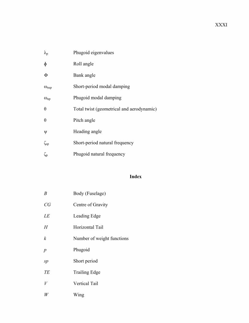
XXXI

λp Phugoid eigenvalues ɸ Roll angle Φ Bank angle ωnsp Short-period modal damping ωnp Phugoid modal damping θ Total twist (geometrical and aerodynamic) θ Pitch angle ψ Heading angle ζsp Short-period natural frequency ζp Phugoid natural frequency

Index

B Body (Fuselage) CG Centre of Gravity LE Leading Edge H Horizontal Tail k Number of weight functions p Phugoid sp Short period TE Trailing Edge V Vertical Tail W Wing

XXXII

WB Wing Body WBH Wing Body Horizontal Tail WBT Wing Body Tail

INTRODUCTION

For airplanes, one of the main concerns is that the vehicle is easily controllable and

maneuverable. Two different aspects are important: controllability and stability, concepts

which are not equivalent. A high number of airplanes considered excellent in terms of their

characteristics (dimensions, weights and performances) show a slight lateral instability called

divergence spiral. Instability is no longer a problem thanks to the fly–by–wire system which

replaces the conventional manual flight control. The automatic signals sent by the aircraft's

computers allows to perform functions without needing the pilot's input, as in systems that

automatically help stabilize the aircraft.

Today, generation of mathematical models needed to represent the various dynamics

phenomena are very important in the aerospace field. Such mathematical models are

conceived in many disciplines related to aerospace engineering. Major aerospace companies

have developed their own codes to estimate the aerodynamics characteristics and aircraft

stability in conceptual phase.

In parallel, universities have developed various codes for educational and research purpose.

At LARCASE laboratory, where the projects are focused mainly in aeronautical field, a code

called FDerivatives was dedicated to the analytical and numerical calculations of the

aerodynamics coefficients and their corresponding stability derivatives. This code is written

in MATLAB and has a user friendly graphical interface. Strongly linked to the aircraft

geometry and flight conditions, the aerodynamic derivatives are needed for its stability and

control analysis. Given the complexity and the scope of this project, the research was

performed on the aircraft flying in the subsonic regime. Presagis gave the « Best Simulation

Award » to the LARCASE laboratory for FDerivatives and data FLSIM applications.

This code can be used as a design tool, and new methods for aircraft's analysis have been

added, to be able to complete the aim of this thesis. The weight functions method was applied

2

to study the stability and a numerical application of the continuity algorithm is presented to

improve the flight envelope for minimum airspeeds.

Figure 0.1 The main methods used for aircraft analysis

This research thesis is part of two projects. The first project was initiated by CAE Inc. and

the Consortium for Research and Innovation in Aerospace in Quebec (CRIAQ) and the

second project was funded by NATO in the frame of the NATO RTO AVT–161 program,

«Assessment of Stability and Control Prediction Methods for NATO Air and Sea Vehicles ».

The latter project was awarded the « RTO Scientific Achievement Award 2012 », the most

prestigious award that has been offered to the AVT-161 NATO research team.

Three aircraft models were analyzed in this paper:

• The Hawker 800XP, a midsize twin–engine corporate aircraft with low swept–back

one–piece wing, a high tail plane and rear–mounted engines;

Aircraft's geometry

FDerivatives code: calculation of aerodynamic coefficients

and their derivatives (Hawker 800XP and X-31)

Weight Functions Method: stability analysis

• stable aircraft (Hawker 800XP and X-31)

• unstable aircraft (HIRM) - added control law

Continuity algorithm: improve the flight envelope using a control law

(HIRM)

3

• The X–31 aircraft, designed to break the « stall barrier », which allows it to fly at

angles of attack that would typically cause an aircraft to stall resulting in loss of

control; and

• The High Incidence Research Model (HIRM) of a generic fighter aircraft

implemented in Aero-Data Model In Research Environment (ADMIRE) code,

developed by the Swedish Defense Research Agency.

Four of the five journal papers presented in this thesis use the in-house results obtained with

FDerivatives code. The first two papers were written in collaboration with my colleagues at

the LARCASE laboratory. My contributions as main author, as well as the contributions of

colleagues to each article, are specified in the Objectives and Originality section. As Ph.D.

advisor, Dr. Botez is the co–author of these papers.

In the first paper, the aerodynamics and stability coefficients are estimated based for the

Hawker 800XP, a mid-size corporate aircraft, using the new in-house FDerivatives code.

These coefficients were further validated with the geometrical and experimental flight test

data provided by CAE Inc.

The second paper was also realized by use of the same in-house code, but for a different

aircraft configuration. The X–31 aircraft is a delta-wing configuration that was tested in the

Low–Speed Wind Tunnel of the German–Dutch Wind Tunnels (DNW–NWB). By taking

into account a minimum number of geometrical parameters delivered by German Aerospace

Center (DLR), the remaining geometrical data were calculated to complete the database of

the aircraft’s geometry. The aerodynamics and their stability coefficients, as well as the total

side force, rolling and yawing moments’ coefficients were validated with wing tunnel test

data. The longitudinal behavior of the aircraft about the pitch–axis reference frame was also

analyzed.

We began with a code based on the geometrical parameters of an airplane, and built on that

with a new method called the weight functions method. This method was applied for

4

longitudinal and lateral–directional dynamics studies in the last three papers. This method

extends the FDerivatives code so that it can produce a complex analysis of aircraft stability,

as a design tool, completed with the continuity algorithm used to estimate flight envelope

minimum airspeeds.

The development of a new interface that can unify FDerivatives code with the weight

functions method and a continuity algorithm could be a future project at LARCASE. Before

embarking on this new project it will be necessary to validate how to choose the weight

functions for similar aircraft configurations (classical configuration wing-body-tail, as in the

Hawker 800XP, a wing-delta configuration, as in the X-31, and a wing-delta configuration

equipped with thrust vectoring capability, as with the HIRM). Therefore, a minimum of three

different aircraft will analyzed with the weight functions method.

The weight functions method presented here is similar to the Lyapunov method, except for

how the weight functions are defined. In the Lyapunov method the functions are chosen

simultaneously, while for the weight functions method each weight function is selected step

by step. Numerical results are presented in the last three papers.

The continuity algorithm is described in this thesis as the last step in our analysis, and

numerical results are presented for HIRM aircraft in order to estimate the minimum airspeeds

of the flight envelope for the model stabilized by using the control law.

This thesis is organized as follows: A literature review is presented in Chapter 1 after a

detailed Introduction. A introduction to the first paper and to the FDerivatives code is

provided in Chapter 2, including the detailed results and description of the FDerivatives code

for the Hawker 800 XP configuration. The second paper is fully presented in Chapter 3. The

weight function and the handling qualities methods are introduced and presented in Chapter 4

(for the X-31 aircraft), Chapter 5 (for the Hawker 800 XP) and Chapter 6 (for HIRM model

aircraft). General conclusions and further work recommendations complete this thesis.

5

The following sections explain the objectives and the originality of the proposed work and

the applied theory is also summarized. A detailed introduction to the FDerivatives code, how

it works and its structure is presented. Stability analysis is covered in Section 0.5, where the

theory is developed for the weight functions method, the handling qualities method and the

continuity algorithm, with numerical results applied to HIRM aircraft.

0.1 Objectives and originality

The main objective of this thesis is to perform a more complete analysis of an aircraft in

subsonic regime as a design tool, based on geometrical parameters. Its originality lies in the

methods chosen to analyze the stability of three real aircraft, sustained with numerical

results. In order to accomplish this task, this research treats three categories:

• The new in–house FDerivatives code, developed at LARCASE laboratory, designed

to calculate the aerodynamic coefficient values and their derivatives. The results have

been validated numerically for two different aircraft configurations: the Hawker

800XP and X-31 aircraft.

• The Weight Functions Method (WFM) is used as a design tool to determine an

aircraft’s stability. The method was applied on the Hawker 800XP, the X-31 and a

High Incidence Research Aircraft Model (HIRM) aircraft.

• A continuity algorithm is used to estimate the minimum airspeeds for longitudinal

dynamics of the HIRM aircraft, stabilized with the control law.

To achieve this goal, the flight test data provided by CAE Inc for the Hawker 800XP and the

experimental results provided by the Low–Speed Wind Tunnel of the German–Dutch Wind

Tunnels (DNW–NWB) for the X–31 model have been invaluable. With their data, along with

the real airfoils’ coordinates, the FDerivatives code could be validated. The High Incidence

Research Aircraft Model (HIRM) developed by the Swedish Defense Research Agency and

implemented in Aero-Data Model In Research Environment (ADMIRE) code was used to

validate the WFM and the continuity algorithm. The flight configurations were selected

because they are among the flight conditions for Cat. II Pilot Induced Oscillation (PIO)

6

criteria validation, performed on the FOI aircraft model presented in the PIO Handbook by

the Group for Aeronautical Research and Technology in Europe, Flight Mechanics/Action

Group 12.

The first step was to help to define and complete the FDerivatives code, conceived and

developed to calculate the aerodynamic coefficients and static/dynamic stability derivatives

of an aircraft in subsonic regime, based on its geometrical data. FDerivatives is an

implementation in MATLAB of the DATCOM method, improved for estimating the pitching

moment coefficient, the lift curve slope, and for the calculus of the aerodynamic parameters

for airfoils specified by NACA. This will be detailed in Section 0.4, with the code description

and its improvements.

The first model implemented and tested in FDerivatives code was the geometry of a Hawker

800XP, thoroughly checked and verified for missing data (such as airfoils, fuselage

coordinates, among others). Each function contained in the DATCOM method was then

implemented in MATLAB with the relevant improvements. The task required teamwork, and

a large part of the implementation of the methods in FDerivatives code was accomplished by

Mr. Dumitru Popescu.

The checking and completing of the geometry in order to implement it in Digital DATCOM

and validate its first phase with flight test data was part of my work. Once the geometry was

validated I switched to the MATLAB code. I first verified all the functions written earlier by

my team, and then I continued to implement the derivatives functions regarding the sideslip,

the roll rate and the pitch moment coefficient.

While the FDerivatives code was being completed for a typical wing-body-tail configuration,

the canard model was implemented. The graphical interface was radically changed; this

change can be seen in the second journal publication. The results were validated using the X–

31 aircraft geometry and the wind tunnel experimental data for Mach number 0.18 at Sea

7

Level. This model was also tested in Digital DATCOM, where the wing was implemented as

a horizontal tail and the canard as the wing parameters.

Once the code was completed and validated for two real aircraft, with different

configurations, the second step was to choose and apply a new stability method called the

Weight Functions Method. This new method replaces the classical Lyapunov stability

criterion based on finding a Lyapunov function. Finding a Lyapunov function is not simple

task and it is not always guaranteed. The Lyapunov method is very useful, however, when

the linearization around the point of equilibrium leads to a matrix of evolution with

eigenvalues having zero real parts.

The difference between these two methods is that the WFM finds one function at a time, with

their number equal to the number of the first-order differential equations. The WFM’s basic

principle is to find three positive weight functions for a system with four first-order

differential equations, where the fourth weight function is a constant, imposed by the user.

Aircraft stability is determined from the sign of the total weight function; this sign should be

negative for a stable aircraft. The Root Locus method was used to validate this new method.

The first two aircraft models were stable, and so a third, nonlinear model was used. For

HIRM aircraft the WFM was applied to the original aerodynamics model implemented in

ADMIRE code, as well as for the model stabilized with control laws, defined for longitudinal

and lateral motions. Starting with its flight envelope, which has a non-typical shape, the

continuity algorithm was chosen to improve this envelope for a HIRM model stabilized with

the control law.

0.2 Background theory on aircraft modelling

The theoretical concepts on which the subsequent chapters are based are next described. An

aircraft is represented in Figure 0.2 in the body axis system, which is fixed in the aircraft’s

8

centre of gravity. The x– axis is positive forward through the nose, the y– axis is positive out

through the right wing and the z– axis is positive upward.

Figure 0.2 Body axis system of the aircraft

Table 0.1 presents the applied forces and moments, as well as the angular velocities and

positions found in the reference axis system.

Table 0.1 Notations for speeds, positions, moments of inertia, forces and moments in an aircraft’s reference axis

Axis Linear

speed

Angular

speed

Angular

position

Moment of

inertia

Moment

applied

Force

applied

x u p

roll rate

φ

roll angle

Ix

roll inertia L X

y v q

pitch rate

θ

pitch angle

Iy

pitch inertia M Y

z w r

yaw rate

ψ

yaw angle

Iz

yaw inertia N Z

The six equations of forces and moments (Etkin et al., 1996) used to analyze the Hawker

800XP and X-31 aircrafts are given by eq.(0.1):

9

( )( )( )

( ) ( )( ) ( )

( ) ( )2 2

sin

cos sin

cos cos

x z y xz

y xz x z

z xz y x

X m u qw rv g

Y m v ru pw g

Z m w pv qu g

L I p qr I I r qp I

M I q p r I pr I I

N I r qr p I pq I I

θθ φθ φ

= + − −

= + − −

= + − −

= + − − +

= + − + −

= + − + −

(0.1)

Three other equations are required to relate the angular rates p, q and r to the Euler angles: φ,

θ and ψ (see eq.(0.2)).

sin

cos cos sin

cos cos sin

p

q

r

φ ψ θθ φ ψ θ φψ φ θ θ φ

= −

= +

= −

(0.2)

The Euler rates are defined in eq.(0.3)

( )

sin tan cos tan

cos sin

sin cos sec

p q r

q r

q r

φ φ θ φ θθ φ φψ φ φ θ

= + +

= −= +

(0.3)

The model described by eqs (0.1), (0.2) and (0.3) was used to study the stability of two

different aircraft configurations, for the Hawker 800XP and the X31.

The first aircraft studied in this paper is the Hawker 800XP, a midsize twin–engine corporate

aircraft with low swept–back one–piece wings, a high tailplane and rear–mounted engines,

for which the maximum Mach number is equal to 0.9. This aircraft operates in the subsonic

and transonic regimes. Three views of the Hawker 800XP aircraft are represented in the

OXYZ reference system (Figure 0.3).

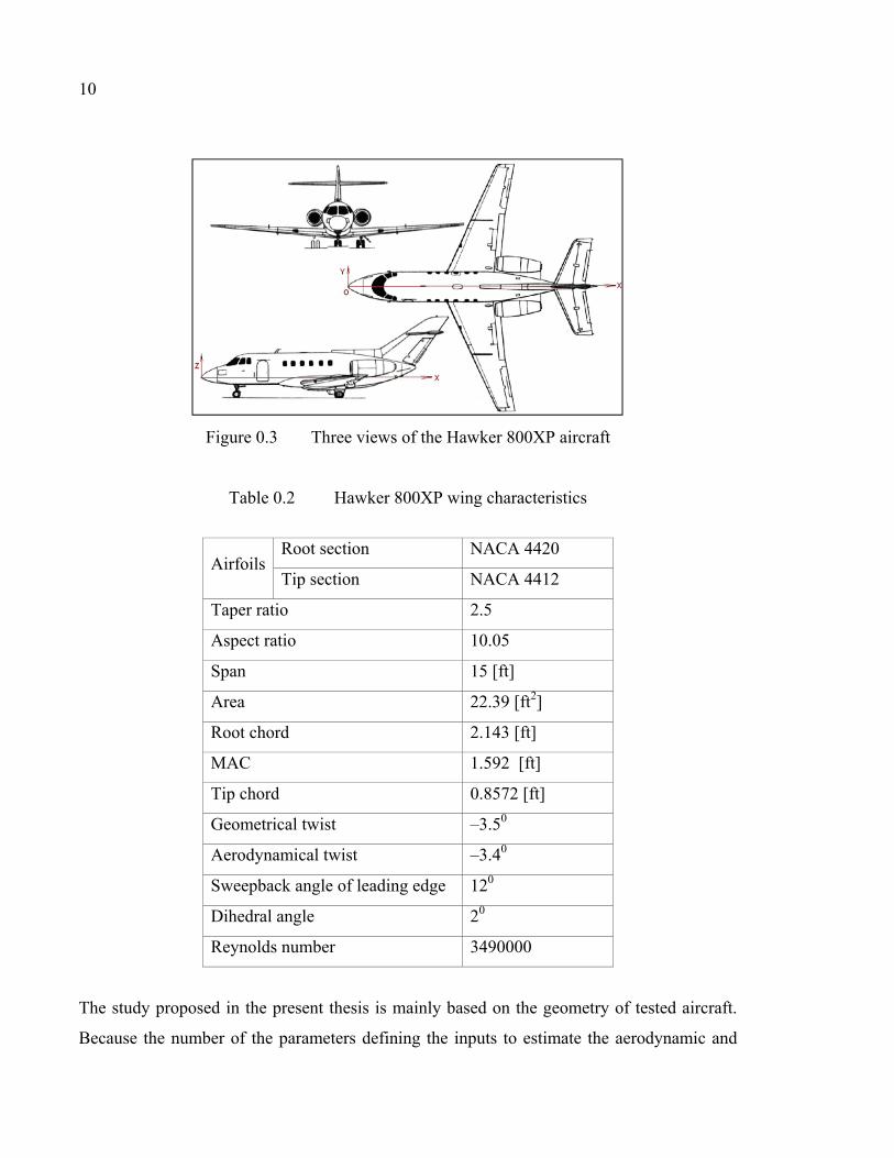
10

Figure 0.3 Three views of the Hawker 800XP aircraft

Table 0.2 Hawker 800XP wing characteristics

Airfoils Root section NACA 4420

Tip section NACA 4412

Taper ratio 2.5

Aspect ratio 10.05

Span 15 [ft]

Area 22.39 [ft2]

Root chord 2.143 [ft]

MAC 1.592 [ft]

Tip chord 0.8572 [ft]

Geometrical twist –3.50

Aerodynamical twist –3.40

Sweepback angle of leading edge 120

Dihedral angle 20

Reynolds number 3490000

The study proposed in the present thesis is mainly based on the geometry of tested aircraft.

Because the number of the parameters defining the inputs to estimate the aerodynamic and

11

stability coefficients in FDerivatives code is very large, it was sometimes necessary to

estimate the missing geometrical data. These parameters are detailed in the next section.

The X–31 aircraft, the second aircraft analyzed, was designed to break the « stall barrier »,

allowing it to fly at angles of attack that would typically cause an aircraft to stall resulting in

loss of control. The X–31 employs thrust vectoring paddles which are placed in the jet

exhaust, allowing the aircraft’s aerodynamic surfaces to maintain their control at very high

angles. For its control, the aircraft has a small canard, a single vertical tail with a

conventional rudder, and wing leading–edge and trailing–edge flaps.

The X–31 aircraft also uses computer controlled canard wings to stabilize the aircraft at high

angles of attack. The stall angle at low Mach numbers is α = 300. The X–31 model geometry

(Henne et al., 2005) was given by the DLR, at the scale 1:5.6 (Table 0.3) at the AVT–161

meeting.

Table 0.3 Geometrical parameters

Fuselage length 1.725 m

Wing span 1.0 m

Wing Mean Aerodynamic Chord (MAC) 0.51818 m

Wing reference area 0.3984 m2

Wing sweep angle, inboard 57 deg

Wing sweep angle, outboard 45 deg

Canard span 0.36342 m

Canard reference area 0.04155 m2

Canard sweep angle 45 deg

Vertical Tail reference area 0.0666 m2

Vertical Tail sweep angle 58 deg

12

The main part of the X–31 model is a wing–fuselage section with eight servo-motors for

changing the angles of the canard (δc), the wing Leading–Edge inner/outer flaps (δLei / δLEo),

wing Trailing–Edge flaps (δTE) and the rudder (δr) (Rein et al., 2008). The variation of these

angles, for each control surface, is given as:

o Canard: –700 ≤ δc ≤ 200,

o Wing inner Leading-Edge flaps: –700 ≤ δLEi ≤ 00,

o Wing outer Leading-Edge flaps: –400 ≤ δLEo ≤ 00,

o Wing Trailing-Edge flaps: –300 ≤ δTE ≤ 300,

o Rudder: –300 ≤ δr ≤ 300.

The wing parameters were introduced in Digital DATCOM for the horizontal tail and the

canard as a wing.

The third model in this study is the HIRM (High Incidence Research Model) (Admirer4p1),

(Lars et al., 2005), (Terlouw, 1996) of a generic fighter aircraft. This aircraft model has an

envelope defined by a Mach number between 0.15 and 0.5 and altitude of between 100 and

20,000 ft for the following angles: the angle of attack α = [-10 to 30] degrees, sideslip angle β

= [-10 to 10] degrees, elevon angle δe = [-30 to 30] degrees, canard angle δc = [-55 to 25]

degrees, and rudder angle δr = [-30 to 30] degrees.

The aerodynamics coefficients were obtained based on wind tunnel and flight tests

(Admirer4p1) for a model « ... originally designed to investigate flight at high angles of

attack ... but [that] does not include compressibility effects resulting from high subsonic

speeds. » (Terlouw, 1996, p 21).

13

Figure 0.4 Body axes system of an HIRM aircraft

Table 0.4 Summary of the HIRM aircraft's geometrical data, along with aircraft mass

and mass distribution data

Parameters Numerical values [Units]

Wing area S 45 m2

Wing span b 10 m

Wing Mean Aerodynamic Chord c 5.2 m

Mass m 9100 kg

x-body axis moment of inertia Ix 21000 kgm2

y-body axis moment of inertia Iy 81000 kgm2

z-body axis moment of inertia Iz 101000 kgm2

xz-body axis product of inertia Ixz 2500 kgm2

zeng -0.15 m

xcg 0.25 c

The HIRM aircraft was evaluated (see Figure 0.4 and Table 0.4) based on the nonlinear

system of equations given by eq.(0.4):

14

( )

( )( )

( ) ( )( ) ( ) ( )( ) ( ) ( )

00

2 21 2

1 2

sin

sin cos

cos cos

s

D E

Y

L

l x xz y x

m ATP ATP E x y xz z x

n ATP ATP E x z xz x y

q S C mg F m u qw rv

q S C mg m v ru pw

q S C mg m w pv qu

q S bC I p I r pq I I qr

q S c C Z Z F I q I r p I I rp

q S bC Y Y F I r I p qr I I pq

p q

ρθρ

φ θφ θ

φ

− + = + −

− + = + −

+ = + −

− = − + − −

− + + = − − − −

− − + = − − − −

= +

( )

( )

( )( )

( )( )

in cos tan

cos sin

sin cos

coscos cos cos cos sin sin cos

cos sin cos sin sin

sin cos sin sin sin cos cos

sin sin cos cos sin

sin cos sin cos cos

r

q r

q r

x u v

w

y u v

w

z u v w

φ φ θ

θ φ φφ φ

ψθ

ψ θ ψ θ φ ψ φψ θ φ ψ φ

ψ θ ψ θ φ ψ φψ θ φ ψ φ

θ θ φ θ φ

+= −

+=

= + − +

+ +

= + + +

+ −= − + +

(0.4)

0.3 DATCOM method

The aircraft geometrical parameters are: wing span, Mean Aerodynamic Chord (MAC),

sweep back angle of the leading edge, reference surface, weights, thrust, speeds (minimum

control speed on the ground (VMC Ground), take–off safety speed (V2) and landing

reference speed or threshold crossing speed (VREF), length, height, position of the

gravitational centre, position and number of the engines, among numerous others.

The required inputs are estimated as a function of the airfoils’ coordinates, while the aircraft

geometrical data is given in 3D coordinates.

15

A. Digital DATCOM limitations (Finck et al., 1978)

An aircraft’s stability is measured in terms of its derivatives - the rate of change of one

variable with respect to another variable. The DATCOM method, implemented in

FORTRAN and called the Digital DATCOM code presents several operational limitations

(Finck et al., 1978), (Williams et al., 1979a) (see Table 0.5).

• « The forward lifting surface is always input as the wing and the aft lifting surface as the horizontal tail. This convention is used regardless of the nature of the configuration.

• Twin vertical tail methods are only applicable to lateral stability parameters at subsonic speeds.

• Airfoil section characteristics are assumed to be constant across the airfoil span, or as an average for the panel. Inboard and outboard panels of a cranked or double–delta planform can have their individual panel leading edge radii and maximum thickness ratios specified separately.

• If airfoil sections are simultaneously specified for the same aerodynamic surface by an NACA designation and by coordinates, the coordinate information will take precedence.

• Jet and propeller power effects are only applied to the longitudinal stability parameters at subsonic speeds. Jet and propeller power effects cannot be applied simultaneously.

• Ground effect methods are only applicable to longitudinal stability parameters at subsonic speeds.

• Only one high lift or control device can be analyzed at a time. The effect of high lift and control devices on downwash is not calculated. The effects of multiple devices can be calculated by using the experimental data input option to supply the effects of one device and allowing Digital DATCOM to calculate the incremental effects of the second device.

• Jet flaps are considered to be symmetrical high lift and control devices. The methods are only applicable to the longitudinal stability parameters at subsonic speeds.

• The program uses the input namelist names to define the configuration components to be synthesized. For example, the presence of namelist HTPLNF causes

16

Digital DATCOM to assume that the configuration has a horizontal tail. » (Finck et al., 1978, p 17)

Table 0.5 DATCOM method limitations Source: Finck et al. (1978, p 6)

17

B. Classical aircraft configurations Wing – Body – Tail and Canard

This DATCOM reference treats the classical body–wing–tail stability and geometry

including control effectiveness for a variety of high–lift/control devices. The outputs for the

high–lift/control devices are usually expressed in terms of incremental effects due to control

surface deflections.

Digital DATCOM code is applied to the classical aircraft, including canard configurations, in

order to estimate the following characteristics:

Static stability characteristics. In Digital DATCOM, where the semi–empirical

DATCOM methods are computed, the longitudinal and the lateral–directional stability

derivatives have been calculated in the stability axis system. The outputs are: the normal

force CN and the axial force CA coefficients, the lift, drag and moment coefficients CL,

CD, and Cm ,as well as their corresponding longitudinal derivatives CLα, Cmα, Cyβ, Cnβ and

Clβ.

Dynamic stability lift, pitch, roll and yaw derivatives CLq, Cmq, Clp, Cnp, Clr, Cnr, , and .

High–lift and control characteristics including jet flaps, split, plain, single slotted,

double slotted, fowler and leading edge flaps and slats, trailing edge flap controls and

spoilers.

Trim data, which can be calculated only for subsonic speeds, where Cm = 0. The trim

option is available for the first mode configurations, as they have a trim control device

on the wing or horizontal tail, and for the second mode configurations, where the

horizontal tail is all–movable.

0.4 FDerivatives code: Description and improvements

With its projects focused mainly in the aerospace field, LARCASE identified the need to

develop a new code for educational and research purposes. This new code, called

FDerivatives, is dedicated to the analytical and numerical calculation of the aerodynamics

18

coefficients and their corresponding stability derivatives. FDerivatives is written in

MATLAB and has a user-friendly graphical interface. Strongly linked to aircraft geometry

and flight conditions, the aerodynamic coefficients and derivatives are needed for aircraft

stability and control analysis. Given the complexity and scope of this project, the research

was limited to aircraft flying in the subsonic regime.

C. Description of the FDerivatives code

The model implemented in the new FDerivatives code is based on the methodology used in

the DATCOM procedure (Williams et al., 1979a) for calculating the aerodynamic

coefficients and their stability derivatives for an aircraft. The main advantage of this new

code is the estimation of the lift, drag and moment coefficients and their corresponding

stability derivatives by use of relatively few aircraft geometrical data: area, aspect ratio, taper

ratio and sweepback angle for the wing and for the horizontal and vertical tails. In addition,

the airfoils for the wing, the horizontal and vertical tails, as well as the fuselage and nacelle

parameters, are designed in a three–dimensional plane.

A logical block diagram is presented in Figure 0.5, which shows how the code works, as a

function of the chosen configuration. The methods presented as a function of Mach number

for a WBT configuration are also given for the other two configurations WB and W in the

same four regimes: low-speed, subsonic, transonic and supersonic. The graphical interface is

designed to allow the user to select the desired configuration for the calculation of the

aerodynamic coefficients and stability derivatives.

19

Figure 0.5 Logical diagram of the new FDerivatives code

In the FDerivatives code, the Reynolds number and the airflow speed over the aircraft are

calculated by considering a theoretical atmospheric model such as the model defined by the

International Civil Aviation Organization (ICAO). This model is an ideal one, in which the

atmosphere is divided into seven different layers, with a linear distribution of temperature.

The main window of the graphical interface is presented in Figure 0.6. The flight

characteristics (altitude, Mach number and angle of attack), the type of the planform

(straight–tapered or non-straight–tapered wing or canard) and the configuration, ,Wing,

Wing–Body or Wing–Body–Tail must be defined before the outputs can be calculated.

20

Figure 0.6 Main window of the graphical interface for the FDerivatives code

Two types of input data are needed for the program. The first set are the geometrical

parameters defining the various components of an aircraft’s wing, fuselage and nacelles,

horizontal and vertical tails. The number of parameters is dictated by the geometry of each

element, and the input done manually, through the « Airplane Geometry » graphic of the

Stability Derivatives’ main window software. The second set of data is composed of the

coordinates of contour points, taken at representative locations on the surfaces, as well as

contact points of the contour of the fuselage and nacelles. A function is responsible for their

automatic import from Excel spreadsheets. The input parameters needed to calculate the

aerodynamic coefficients and their stability derivatives are described in Tables 0.6 and 0.7.

21

The input data for the fuselage and nacelles are coordinates taken as contour points in two

perpendicular planes: the horizontal plane parallel to the axis of reference of the aircraft and

the vertical plane containing the axis of symmetry. These data are used for calculating the

geometrical parameters required for asymmetric fuselage modeling.

Table 0.6 Inputs for Wing/Canard and Horizontal/Vertical Tail’s geometry Aspect ratio – AW = b2 /SW

Taper ratio – λW

Reference area [ft2] – SW

Quarter chord sweep angle [0] – (Λc/4)W

Dihedral angle [0] - ΓW

Airfoils given for Root, MAC and Tip section in 3D coordinates

Parameters to estimate the Wing/Canard and Horizontal/Vertical Tail’s geometry

Span [ft] – bW

Root chord [ft] – crW

Tip chord [ft] – ctW

Mean Aerodynamic Chord [ft] – c

Lateral position of the MAC [ft]

Sweepback angle at leading edge [0] – ΛLE

Sweepback angle at 25% chord line [0] – Λc/4

Sweepback angle at 50% chord line [0] – Λc/2

Sweepback angle at trailing edge [0] – ΛTE

Twist of tip respect to root, negative for washout [0] – θ

Span of the exposed surface [ft] – beW

Root chord of exposed surface [ft] – cRe

Tip chord of exposed surface [ft] – cTe

Area of exposed surface [ft2] – (Se)W

Sweepback angle of the exposed surface [0] – Λ(LE)We

Aspect ratio of exposed surface – AWe

22

Mean Aerodynamic Chord of the exposed surface [ft] – Wec

Lateral position of the MAC for exposed surface [ft]

Twist of tip respect to root, for exposed surface [0] – θWe

Sweepback angle at leading edge for exposed surface [0] – Λ(LE)We

Sweepback angle at 25% chord line for exposed surface [0] – Λ(c/4)We

Sweepback angle at 50% chord line for exposed surface [0] – Λ(c/2)We

Sweepback angle at trailing edge for exposed surface [0] – Λ(TE)We

Table 0.7 Inputs for fuselage parameters

Body section – circular or elliptical

Nose type – cone or ogive

Forebody – conical or parabolic profile

After body – conical or parabolic profile

Body length [ft]

Position of the gravity centre on x-axis [ft]

Position of the gravity centre on z-axis [ft]

Body coordinates in XOY plane and XOZ plane

Number of nacelles

Position Xo of the nacelle on x-axis [ft]

Nacelle length [ft] -

Nacelle coordinates in XOY plane and XOZ plane

Other usefully dimensions

Exposed wetted area of body (isolated body minus surface area covered by the wing at

wing-body junction) [ft2] – (Ss)e

Maximum fuselage diameter [ft] – d

Maximum cross-section area – SB

Lateral fuselage area – SSe

Body base area – Sbase

Body side area – SbS

23

Total body volume – VB

Wetted or surface body area excluding base area of wing at root – Ss

The new code is organized into several sub-directories, all grouped in a root directory called

FDerivatives_Matlab. Figure 0.7 shows the subdirectories and part of the contents of the root

directory of the code. Apart from sub-directories, this directory contains all the main

MATLAB functions: the FDerivatives.m function which manages the main graphics window

and the rest of the functions for calculating the aerodynamic coefficients and their stability

derivatives.

Figure 0.7 Root directory of the FDerivatives code

The subdirectories and their destinations are described below:

24

• Database folder contains all the text files containing the data obtained from the chart

scanning;

• Geometry folder keeps all the functions, is of secondary in importance in the

algorithm’s operation;

• Input_Data folder is reserved for the parameters from the Excel data files required

for the derivative calculation;

• Output folder represents the destination of the results at the end of program; and

• Photos folder stores the pictures, logos and designs used by the graphical interface.

In addition to the inputs of the Digital DATCOM code, FDerivatives code takes into account

the aerodynamic contributions of nacelles, without any restrictions on their position relative

to the fuselage or wing. However, for a given aircraft, the code considers only an even

number of nacelles, attached either to the fuselage or to the wings, with no possibility of a

combined arrangement (as in the Lockheed L1011 aircraft, for example, where the

contribution of the third engine’s nacelle, located on the dorsal part of the fuselage, is

neglected).

For canard configuration, the wing is treated as the horizontal tail, while the canard is treated

as the main wing. Neither the FDerivatives nor the Digital DATCOM code treat aircraft with

three lifting surfaces, as DATCOM’s methods lack that capability. By three lifting surfaces,

we refer here to airplanes equipped with two main wings, one above the other (the biplane

model), and aircraft with a main conventional wing, horizontal tail located at the rear and a

canard in addition. The codes do not treat the winglets or vertical stabilizers with more than

two lifting surfaces.

D. Improvements of the FDerivatives code to Digital DATCOM

From a methodological point of view, the new methods implemented in FDerivatives code

and presented in this thesis discus a qualitative approach. These methods promote the

25

approaches that we have used to produce a modern, user-friendly tool for calculating

aerodynamic coefficients and stability derivatives.

For the main functions, a general model to implement all the calculation methods was

developed and used in the new code. This model allows for easy replacement of the

methodologies implemented, including adding new methods, and simplifies the debugging

process.

Compared to Digital DATCOM’s applicability limits, the FDerivatives code adds several

enhancements. The possibilities of calculating have been extended to wings with variable

airfoils along the span and negative sweepback. Different approaches to calculate the drag

and pitching moment of the aircraft allow the results for

the drag coefficient to be refined, and significantly improve the coefficient of pitching

moment results. The improvements added to FDerivatives code versus Digital DATCOM

code are detailed in the paragraphs that follow.

D.1. Pitching moment estimation for Wing-Body configuration in Digital DATCOM code

The solution presented and used in Digital DATCOM code for the calculus of the pitching

moment estimated as a function of the angle of attack for the WB configuration is presented

in this section. The equation implemented in the code is:

( ) ( ) ( )0m m m mWB L DC C C C= + + (0.5)

where

(Cm0)WB is the zero lift pitching moment coefficient for the WB configuration

(Cm)L is the moment coefficient given by the lift force as a function of the angle of

attack

(Cm)D is the moment coefficient given by the drag force as a function of the angle of

attack

26

In Digital DATCOM code, for WB configuration the terms (Cm0)WB and (Cm)L are estimated

verifying if the applicability criteria of two methods, where the zero lift pitching moment is

estimated with eq.(0.6).

( ) ( ) ( ) ( )( )

( )0 0

0

mo Mm mo mWB W B W

mo M

CC C C

C=

= + (0.6)

where

(Cm0)W is the zero lift pitching moment for the wing alone

(Cm0)B(W) is the zero lift pitching moment coefficient given by the fuselage in the

presence of the wing

(Cm0)M /(Cm0)M=0 is a correction factor, estimated as a function of Mach number

The zero lift pitching moment coefficient given by the fuselage in the presence of the wing

presents an interesting concept. This coefficient is related to the wing position reported to the

fuselage (Multhopp, 1942). Wind tunnel tests prove that (Cm0)B(W) has a linear variation with

the slip angle of the wing and changes significantly with the fuselage volume, while the

longitudinal position of the wing and its height relative to the reference axis of the fuselage

has less influence (Anscombe et al., 1950). The wing position is totally neglected in the

DATCOM method, which causes a relatively large error in estimating the (Cm0)B(W)

coefficient, which in turn may influence the longitudinal stability derivatives calculations,

including the pitching moment slope (Cmα) for the WB configuration.

Method given in DATCOM shows an empiric correlation obtained by a linear regression

between 18 aerodynamics and geometrical parameters, appropriated to the WB configuration.

To apply this method, the DATCOM procedure gives the correlation coefficients for 14

Mach number values, between M = 0.4 and M = 2.5. The Digital DATCOM code applies this

method, making an extrapolation for Mach numbers up to 0.4. The DATCOM procedure

specifies the reduced precision for this method, but does not specify the errors.

27

D.2. Zero lift pitching moment coefficient estimated in FDerivatives code

Given the arguments presented above, the linear regression method is abandoned. Instead,

calculating the pitching moment coefficient given by the fuselage in the presence of the wing

(Cm0) B(W) is replaced with a semi–empirical method developed by the Royal Aeronautical

Society and presented in reference (Etkin et al., 1998). In the FDerivatives code, this

coefficient is calculated for the individual contributions of the wing, and then the fuselage

contribution is added, considering (of course) the interference effects. Its calculation is given

by eq.(0.7):

( ) ( ) ( ) ( )( )

( )0

0 0 0 00 0

m Mm m m mWB W B W

m M

CC C C C

C=

= + + Δ (0.7)

The first term, the zero lift pitching moment coefficient given only by the wing, (Cm0)W, is

calculated based on method 1 described by the DATCOM procedure; this method is valid for

all types of wings that have a the sweepback angle of equal to 45 degrees. The second term,

(Cm0)B(W) (eq.(0.8)), is calculated following analysis of the wind tunnel experimental data,

obtained as a linear function of the angle (iw)0 between the direction of zero lift of the wing

and the reference axis of the fuselage.

( ) ( )( )

( )( )0 0

0

0

term obtained by interpolation

w F Fref m Fm B W

w F F ref

i S lcS CC

i S l cS

=

(0.8)

The term in brackets is obtained by interpolation between the curves shown in Figure 0.8,

and is based on the geometric parameters related to the geometry of the WB configuration,

namely:

c Mean Aerodynamic Chord of the wing;

Sref wing area;

SF surface of the fuselage projection in the horizontal plane;

lF fuselage length;

w fuselage diameter, measured in the horizontal plane at the first quarter of the

28

MAC of the wing;

FS front surface of the fuselage projection in the horizontal plane, measured up the

first quarter of the wing MAC; and

Fl front length of the fuselage, measured in the longitudinal axis between the nose

and the first quarter of the wing MAC.

Figure 0.8 Fuselage effect on the zero lift pitching moment coefficient for the wing-body configuration (median position of the wing)

Source: This figure is a reproduction in MATLAB obtained by digitizing the curves of Figure B.8,2 (Etkin et al., 1998)

In the additional term ΔCm0 of eq.(0.9), the influence of the height position of the fuselage to

the longitudinal axis is included and its values are next given.

0

0.04 high wing

0 median wing

0.04 low wingmC

+Δ = −

(0.9)

The correction of the compressibility effect is given by the ratio (Cm0)M / (Cm0)M=0 and the

value is obtained by interpolation as a function of Mach number, estimated starting at the

curve presented in Figure 0.9.

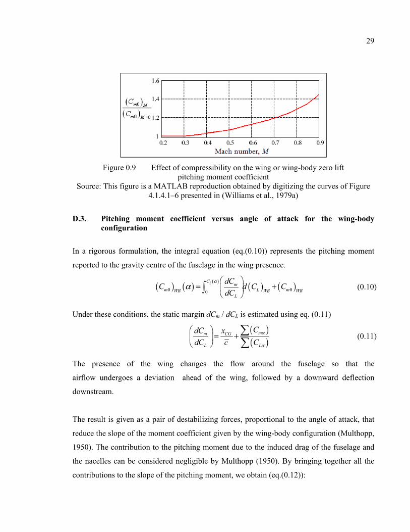
29

Figure 0.9 Effect of compressibility on the wing or wing-body zero lift pitching moment coefficient

Source: This figure is a MATLAB reproduction obtained by digitizing the curves of Figure 4.1.4.1–6 presented in (Williams et al., 1979a)

D.3. Pitching moment coefficient versus angle of attack for the wing-body configuration

In a rigorous formulation, the integral equation (eq.(0.10)) represents the pitching moment

reported to the gravity centre of the fuselage in the wing presence.

( ) ( ) ( ) ( ) ( )0 00

LCm

m L mWB WB WBL

dCC d C C

dC

αα

= +

(0.10)

Under these conditions, the static margin dCm / dCL is estimated using eq. (0.11)

( )( )

mm CG

L L

CdC x

dC c Cα

α

= +

(0.11)

The presence of the wing changes the flow around the fuselage so that the

airflow undergoes a deviation ahead of the wing, followed by a downward deflection

downstream.

The result is given as a pair of destabilizing forces, proportional to the angle of attack, that

reduce the slope of the moment coefficient given by the wing-body configuration (Multhopp,

1950). The contribution to the pitching moment due to the induced drag of the fuselage and

the nacelles can be considered negligible by Multhopp (1950). By bringing together all the

contributions to the slope of the pitching moment, we obtain (eq.(0.12)):

30

( ) ( ) ( ) ( ) ( ) ( ) ( ) ( ) ( ) ( )m m m m mBN W D W B B W B NC C C C Cα α α α α ε ε+ +

= + + + (0.12)

The sum of the lift contributions generated by the fuselage and the nacelles are given by the

term (Cmα)BN. For a body of revolution, the slope of the pitching moment coefficient is given

by eq.(0.13), and can be applied to the fuselage as well as to the nacelles.

( ) ( ) ( )

0

0

2 1 1

0

2 4 f

c

lx

m m d mF F x

k k dSC x x dx rc x x dx rad

V dx Vαα η −−

= − + − (0.13)

The contribution due to the wing’s drag is given by eq.(0.14):

( ) ( ) ( ) 2 Am LW D W

zC C

eA cα π = −

(0.14)

where:

(CL)W is the lift coefficient of the wing;

e is Oswald efficiency factor;

A is the wing aspect ratio; and

zA is the vertical distance between the first quarter of wing’s MAC and the aircraft

gravity centre.

The contribution of the lift for the exposed wing in the presence of the fuselage to the slope

of the pitching moment curve with respect to the center of gravity is given by the following

(eq.(0.15)):

( ) ( ) ( ) ( )exposedac rm LW B B W e

r ref

Sx cC n C

c c Sα α+

= −

(0.15)

where:

n is the distance between the wing leading edge at the root and at the gravity centre,

estimated as a function of the root chord (cr);

Sexposed is the exposed area of the wing; and

(CLα)e is the lift curve slope of the exposed wing.

31

'

tan2

e

e

rac acLE

r r r r

cx x d

c c c c

= + Λ

(0.16)

The last term of eq.(0.12) represents the contribution of the free moments due to the fuselage

and the nacelles. For an N numbers of nacelles, this value is given as:

( ) ( ) ( ) ( ) ( ) ( ) ( )m m mB N B NC C N Cα α αε ε ε ε+

= + (0.17)

The calculus method for the individual contributions of the fuselage and nacelles is detailed

in the DATCOM procedure.

The presence of nacelles generally has the effect of moving the aerodynamic centre forward

and providing a negative contribution to the pitching moment coefficient through the lift. As

we have seen, the contribution of the lift of the fuselage to the slope of pitching coefficient is

expressed using eq.(0.13), which can also be applied to the nacelles. As for their effect on the

position of the aerodynamic centre, the implemented method is based on the equation

suggested by Torenbeek (1976), in which the individual contribution of a platform is given

by eq.(0.18).

( )2

ac N Nn

r r ref L WB

x d lk

c c S C α

Δ =

(0.18)

where the proportionality coefficient as a function of the nacelle position by ratio of the wing

or fuselage is:

4 nacelle placed on the wing

-2.5 nacelle placed on the fuselagenk−

=

(0.19)

lN = nacelle length;

dN = maximal diameter of nacelle; and

(CLα)WB = lift curve slope for the WB configuration.

The expression (0.18), multiplied by the number N of the nacelles, is added to eq.(0.16) to

obtain the position of the aerodynamic center xac of the WB configuration.

32

D.4. Pitching moment coefficient for the wing-body-tail configuration

The total pitching moment coefficient for an aircraft is calculated as the sum of two major

contributions (see eq.(0.20)): wing-body-nacelles (Cm)WBN and the horizontal tail contribution

(Cm)H, considering the effects of interferences between the horizontal tail and the fuselage,

given by eq.(0.21) .

( ) ( )m m mWBN HC C C= + (0.20)

where:

( ) ( )CG Hm LH H

x xC C

c c = +

(0.21)

xCG is the longitudinal distance between the centre of gravity and the wing leading

edge at the root;

xH is the longitudinal distance between the first quarter of the horizontal tail’s root

chord and the wing leading edge at the root; and

(CL)H is the horizontal tail lift coefficient calculated in the wing-body presence.

Supplementary results are presented in this section for a simple configuration presented by

Thomas et al., (1957). Because the purpose of this work is to present the improvements

added to FDerivatives code versus the DATCOM method, and implicitly versus the Digital

DATCOM code, the moment coefficient for a third aircraft configuration was tested. The

geometrical data are given in APPENDIX A. The results are presented for Mach number

0.13, Reynolds number of 0.71·106 and aspect ratio AR = 4.

33

Figure 0.10 Pitching moment coefficient versus angle of attack estimated with FDerivatives and Digital DATCOM codes, compared with the

experimental results provided by Thomas et al. (1957)

Figure 0.11 Pitching moment coefficient versus angles of attack for WB and WBT configurations estimated with the FDerivatives code and compared with

experimental results provided by Thomas et al. (1957)

34

For all of the angles of attack presented in Figure 0.10 the pitching moment coefficient

provided by the FDerivatives code is closer to the experimental results. It can be seen that the

Digital DATCOM results are far from the experimental results. Therefore, in Figure 0.11 the

only the FDerivatives code results versus the experimental results are presented, for two

configurations: wing-body and wing-body-tail. It is obvious that the improvements to the

FDerivatives code are found in the accuracy of the results.

E. Estimation of geometrical parameters in FDerivatives code versus Digital DATCOM code

Some of the most important inputs in any code that depends on aircraft geometry are the

airfoil coordinates. The accuracy of their definition may change the results. Because the

DATCOM method has its limitations, the next two sections present the improvements

implemented in FDerivatives code for the airfoil coordinates and the calculus of the airfoil

radius at the leading edge.

E.1. Airfoil coordinates implementation

In Digital DATCOM code, there are three methods to define an airfoil. The first method is

the simplest: a NACA airfoil is defined by giving its standard name.

The second method is to provide an array of values, using the average curvature (the skeleton

of the profile) and the thickness. If this method is selected, then inputs to introduce are the

coordinates of a number of points, up to 50, situated on the curve of the average steepness of

the profile and expressed in an orthonormal frame, with its origin as the leading edge of the

profile. This distance, by definition, is the reference chord of the profile and of the x-axis.

The user must also enter the values of the thickness of the profile corresponding to the

abscissas of the points.

The third method consists of providing an array of values: the ordinates of the upper and

lower surfaces in an orthonormal system with its origin as the leading edge of the profile and

35

the string equal to unity as the axis abscissa. The user must provide the ordinates of a number

of points, up to 100, distributed evenly over the upper and lower profile (50 points for each

surface). In addition, the values of the corresponding abscissa of the upper points should

coincide with the abscissa values of the items on the lower surface.

E.2. Calculus of airfoil radius at the leading edge

The aerodynamic parameters, such as the ideal angle of attack, pitching moment and zero lift

angle of attack, are obtained using the thin airfoils theory. The airfoil lift curve slope clα is

calculated using the method developed by Weber (1955). The next step consists of correcting

the compressibility and viscosity effects.

Weber's method requires the explicit equation of the camber’s curve, the thickness

distribution around the camber and the radius of the leading edge (rLE) of the airfoil as input

data. It is impossible to obtain the analytical equation of the camber curve from the

coordinates of points of the airfoil contour. The Digital DATCOM code approximates it with

a function defined by fragments using a smoothing method. The quality of the smoothing

depends mainly on the optimal choice of contour points.

In the geometric sense, the radius of the leading edge is the radius of the minimum circle

closest to the curve of the airfoil at the leading edge. Called the circle of camber or the

osculating circle, it is located inside the concavity of the profile curve, tangent to the point

defining the curve. In other words, the osculating circle is the best approximation of the

curve in one point, a priori better than the tangent at this point. For a given function y(x),

twice differentiable, the radius of camber R (or the radius of the osculating circle) at any

point is given by eq.(0.22).

32 2

2

2

1dydx

Rd ydx

+ = (0.22)

36

The calculation of the radius of the leading edge using eq.(0.22) requires explicit knowledge

of the analytical expression of the function y(x). We suggest replacing this function y(x) by

the equation of the ellipse that approximates, as closely as possible, the leading edge of the

airfoil. The algorithm implemented in FDerivatives code is based on a non-iterative method

(Fitzgibbon et al., 1996) and perfected by Halĺiř et al. (1998) to identify the equation of the

ellipse, which is a special conic case with the general equation written as:

( ) 2 21 2 3 4 5 6, 0F x y AX a x a xy a y a x a y a= = + + + + + = (0.23)

By adding the condition 4a1a3 – a22 > 0 , eq. (0.23) becomes the ellipse equation. Suppose

that around the leading edge of the airfoil we have N points on its contour. Consider a point

Pi on the airfoil contour and replace the (xi, yi) coordinates in the equation of the ellipse,

eq.(0.23). Since the point Pi is not necessarily on the ellipse, its coordinates satisfy eq.(0.23)

to a residue such that F(xi, yi) = ri, ∈ , where ri is the absolute error.

Over one contour point of the airfoil is close to the ellipse, plus the value of error ri

approaches zero. Because the error ri can take negative values, it is more convenient to use

the positive value obtained by the error square. By calculating the residue ri for each point N

on the contour of the profile and making the sum of their squares, an expression g dependent

on the ellipse’s parameters ai, with i = 1 ÷ 6 , is obtained in the form of eq. (0.24):

( ) ( ) 22 21 6

1 1

,..., ,N N

i i ii i

g a a F x y A r= =

= = = D (0.24)

where D is the matrix of order (N, 6) constructed with the coordinates of N points situated

on the airfoil’s contour:

2 21 1 1 1 1 1

2 2

2 2

1

. . . . . .

1

. . . . . .

1

i i i i i i

N N N N N N

x x y y x y

x x y y x y

x x y y x y

=

D

The approximation problem at the leading edge of an ellipse is reduced by minimizing the

total squared errors (0.24) under the constraint of inequality. The values of the variables ai, i

37

= 1 ÷ 6 bring the function g(a1, ..., a6) to a minimum. They are the parameters of the ellipse

that best match the airfoil contour. In ideal circumstances, when the points N of the profile

simultaneously belong to the ellipse, the total square errors approaches zero. The classical

approach to solving an optimization with nonlinear constrained inequality is the application

of Lagrange’s multipliers method under the conditions of Karush-Kuhn-Tucker. In practice,

taking these conditions into account is complicated, as several possible aspects must be

considered without guaranteeing an optimal solution (Rao, 1996). Rao (1996) used the

invariance property of a conic with respect to multiplication with a scalar, which offers a

simplistic approach that reduces the optimization problem with inequality constraint to an

optimization problem with an equality constraint. According to Rao (1996), multiplying the

expression (0.23) by a real number of a particular value can make the inequality constraint

4a1a3 – a22 > 0 an equality constraint:

21 3 24 – 1a a a = . (0.25)

Using the matrix form, the identity defined by eq.(0.25) can be written in the following form

1T =A CA (0.26)

where C is the square matrix with constant coefficients of order 6 defined by eq. (0.27).

0 0 2 0 0 0

0 1 0 0 0 0

2 0 0 0 0 0

0 0 0 0 0 0

0 0 0 0 0 0

0 0 0 0 0 0

−

=

C (0.27)

Using Lagrange's multipliers method to minimize the function given by eq.(0.24) under its

constraint the function L(λ, A) defined by eq.(0.28) is given, where the parameter λ is a real

number, known as the Lagrange parameter.

( ) ( )2, 1Tλ λ= + −L A DA A CA (0.28)

The equivalent matrix system of equations obtained by applying the gradient operator is

written as:

38

1

T

T

λ =

=

D DA CA

A CA (0.29)

To approach an ellipse, for a minimum number of points N = 5, the system (0.29) admits a

solution set consisting of six pairs (λj, Aj), of which only one minimizes the total squared

error. What can be remarked? The first observation is that the total square error ||DA||2 ,

which can be written using the properties of matrices as eq.(0.30), establishes the equivalence

between the total squared error and the variable λ of the system (eq.(0.29)):

2 T T Tλ λ= = =

I

DA A D DA A CA (0.30)

The second remark relates to the shape of the first equation of system (0.29), which is

actually an equation for eigenvalues λ and eigenvectors (CA). Among the solutions of the

system (0.29), of the six eigenvalues λi, only one is positive and corresponds to the minimal

value of the total squared error expressed by eq.(0.30). This reduces the minimization

problem in searching for the positive eigenvalue whose corresponding eigenvector is

composed by the ellipse’s coefficients that best approximate the curve of the airfoil.

In summary, the smallest positive eigenvalues λ of the matrix M = (DTDC-1) represent the

minimum total square error given by eq.(0.30). Matrix C is a singular matrix because of its

particular shape.

( ) 1 1T

λ−

=C D D CA CA (0.31)

Using eq.(0.31) avoids the singularity problem of matrix C, but introduces a new problem

with a possible singularity of the matrix S = DTD. Theoretically, matrix S is singular if all N

points satisfy the equation for the same ellipse (Rao, 1996).

In practice, because of the inaccuracy of the rounding errors for a large number of points

belonging to an ellipse, matrix S is singular and Fitzgibbon's algorithm can be applied

without problems. This probability rapidly becomes significant for a small number of points,

as in the case of the FDerivatives code, which only uses the coordinates of 11 points from the

39

leading edge of the airfoil. To avoid these singularity problems, we use an approach proposed

by Halĺiř et al. (1998) that divides the matrix S into three sub-matrices of order 3 by the

process:

4 3 2 2 3 2 22

3 2 2 3 2 2 2

2 2 3 4 2 3 2

1 2

2 3

1 2 2, ,

1

T

x x y x y x x y x xy xx

xy xy yx y x y xy x y xy y

x yx y xy y xy y y

=

= = =

S SS

S S

S S S S S S S S S

S S S S S S S S S S S S

S S S S S S S S

(0.32)

The elements of these matrices are given by:

1

m m

Nm mi ix y

i

S x y=

= (0.33)

Next, the authors replace the singular matrix C, associated with condition (0.26), with the

regular matrix C1 (eq.(0.34)), and reduce the matrix M at a 3-dimensional square matrix M1

given by eq.(0.34) (Halĺiř et al., 1998):

1 11 1 1 2 3 2 1

0 0 2

, 0 1 0

2 0 0

T− −

= − = −

M C S S S S C (0.34)

The matrix M1 has two negative eigenvalues and one positive (or zero if all points belong to

an ellipse) which coincide with the only positive eigenvalue of matrix M. It should be noted

that the matrix S3 can be singular only if the N chosen points are collinear.

FDerivatives uses a code, apart from the leading edge, composed of the coordinates of 5

points situated on the upper surface and of 5 points that belong to the lower surface. Initially

the code built the matrix D using the coordinates of 11 points situated at the leading edge.

Next, the code constructs matrices S1, S2, S3 and matrix M1. Finally, the code calculates the

matrix M1 and retains the positive eigenvalues with which the code constructs the

correspondent eigenvector. Once the ellipse equation has been determined, the FDerivatives

code calculates the camber radius at the airfoil’s leading edge, using eq.(0.22). The results for

40

the NACA 65A008 airfoil (Thomas et al., 1957) are presented in Figure 0.12 to verify the

FDerivatives calculations.

Figure 0.12 The ellipse that approximates the leading edge radius for the NACA 65A008 airfoil

Relative error of this method versus the experimental results is given in Table 0.8 for the

NACA 65A008.

Table 0.8 Leading edge radius calculated versus experimental

NACA-TN-4077

(Thomas et al., 1957)FDerivatives code

Digital DATCOM

code

Leading edge radius 0.00408 0.0038 0.00293

Relative error 6.86% 28.18%

Ten other airfoils were tested and the relative errors have been estimated for experimental

versus FDerivatives and Digital DATCOM codes (see Table 0.8). It can be seen that the

method used in our code is better than the method implemented in Digital DATCOM,

because in Digital DATCOM code the results are similar for the 4-digit or 6-series of NACA

41

airfoils with the same maximum thickness as chord percentages. The maximum camber, the

camber position and the location of the minimum pressure coefficient are not considered in

the calculus of the radius airfoil at the leading edge.

Table 0.9 Validation of the method presented above for the leading edge radius estimation

Airfoil Test

value

FDerivatives

code

Digital

DATCOM code

Relative error (vs.

FDerivatives)

Relative error

(vs. Digital

DATCOM)

NACA 1410 0.0110 0.01101 0.01102 -0.09% -0.18%

NACA 2410 0.0110 0.01101 0.01102 -0.09% -0.18%

NACA 63210 0.0770 0.07680 0.01102 0.26% 85.68%

NACA 65210 0.0687 0.06850 0.01102 0.29% 83.95%

NACA 2415 0.0248 0.02480 0.02479 0.0% 0.04%

NACA 4415 0.0248 0.02480 0.02479 0.0% 0.04%

NACA 23015 0.0248 0.02481 0.02479 -0.04% 0.04%

NACA 632615 0.01594 0.01601 0.02546 -0.044% -59.72%

NACA 2418 0.0356 0.03562 0.03570 -0.056% -0.28%

NACA 66206 0.00223 0.00225 0.00397 -0.89% -79.02%

42

0.5 Stability analysis method

This section provides theoretical descriptions of the methods used in the stability analysis:

the Weight Functions Method (WFM), the Handling Qualities Method (HQM) and the

continuity algorithm. The stability analysis results are presented for X-31 aircraft (Chapter

3), for the Hawker 800XP (Chapter 4) and for the HIRM aircraft (Chapter 5). The continuity

algorithm is applied to the HIRM in section 0.4.4, along with the new flight envelope based

on the model with control law. The mathematical formulas for stability derivative

calculations are given in APPENDIX B.

F. Weight functions method (WFM)

In most practical problems, the differential equations that model the behavior of a dynamic

system often depend on one or more parameters. The WFM is more efficient than the

classical Lyapunov function method, since only one function has to be found at a time. The

Lyapunov stability criteria are based on finding a Lyapunov function, which is not simple

and is not always guaranteed. The Lyapunov method is very useful, however, when the

linearization around the point of equilibrium leads to a matrix of evolution with eigenvalues

having zero real parts.

The WFM replaces the classical Lyapunov function-finding problem with a method that finds

a number of weight functions equal to the number of first-order differential equations that

model the system (Stroe, 2008), (Stroe et al., 2008).

Theorem (Stroe, 2008): Let the autonomous system be ( ) , nf x x= ∈x& ¡ and consider the

existence of n positive functions ( )1 2, ,...,k nw x x x of the class C1 in the neighborhood 0x δ≤

of the origin. The function 1

n

k k kk

W x w f=

=

is formed so that the differentials form

43

1

n

k k kk

dV x w dx=

= to be a total exact differential. The stability of the null solution of the

system is given by the following conditions:

¬ If W is a negative-defined function for any solution x(t) of the given system, with

( ) 00x δ< , then the null solution is an asymptotic stable one;

¬ If W is a null function for any solution x(t) of the given system, with ( ) 00x δ< , then

the null solution is a simple stable one; and

¬ If W is a positive-defined function for any solution x(t) of the given system, with

( ) 00x δ< , then the null solution is unstable.

The difference between the two methods is that the Lyapunov method finds all the functions

simultaneously, while the WFM finds one function at a time, with their total number equal to

the number of first-order differential equations.

To better visualize this method, a logical diagram is presented in Figure 0.13 with its basic

principle defined by the following system equation (eq.(0.35)). The coefficients a1i, b1i, c1i,

and d1i, with i = 1 ÷ 4 contain the stability derivatives terms. The x1, x2, x3, and x4 coefficients

represent the system unknowns.

1 11 1 12 2 13 3 14 4

2 11 1 12 2 13 3 14 4

3 11 1 12 2 13 3 14 4

4 11 1 12 2 13 3 14 4

f a x a x a x a x

f b x b x b x b x

f c x c x c x c x

f d x d x d x d x

= + + + = + + + = + + + = + + +

(0.35)

For a definition of this system, a function 4

1k k k

k

W w x f=

= is found, whose signs will be

studied. In the generic model, w1, w2, w3 and w4 are the weight functions that compose the

total function W given by eq.(0.36) :

( ) ( )( ) ( )

1 1 11 1 12 2 13 3 14 4 2 2 11 1 12 2 13 3 14 4

3 3 11 1 12 2 13 3 14 4 4 4 11 1 12 2 13 3 14 4

W w x a x a x a x a x w x b x b x b x b x

w x c x c x c x c x w x d x d x d x d x

= + + + + + + + +

+ + + + + + + + (0.36)

44

Figure 0.13 Logical diagram for the weight functions method

Three of the four functions, wi ,will be positively defined based on the sign of the coefficients

a1i, b1i, c1i, and d1i with i = 1 ÷ 4. The last function will be constant and imposed by the

author, w4 > 0. If the positive weight functions can be well defined, then the sign of the total

function W will be analyzed in order to identify the stability or instability areas of the system.

G. Handling Qualities Method

The handling and flying qualities are described qualitatively and formulated in terms of pilot

opinions by Cooper et al. (1969). These descriptions reveal the properties that describe the

easiness and effectiveness with which an aircraft responds to pilot commands in the

execution of a flight or of mission tasks. Consequently, they tend to be subjective. The

definition for the handling qualities for an aircraft can be paraphrased as: « Handling

qualities are those qualities or characteristics which govern the ease and precision with which

45

an operator is able to perform the tasks required in support of the vehicle role. » (Cooper et

al., 1969)

A distinction between the handling and flying qualities is shown in Figure 0.14, where it can

be seen that they are interdependent and in practice are probably inseparable. The flying

qualities are related to the mission task, while the handling qualities are related to the

description of the short term dynamic response to controls in the execution of flight tasks.

Figure 0.14 Difference between Handling Qualities and Flying Qualities

The handling qualities exact method was used in this thesis to validate the WFM results

obtained for the aircraft stability analysis. Handling qualities involve the study and

evaluation of the aircraft stability and control characteristics for all five of the dynamic

modes of motion that describe the aircraft's response to an initial condition of any origin

(turbulence, control input, etc.).

« Handling qualities criteria typically define a set of dynamic response characteristics of the vehicle that influence the operator-mission performance. Examples of criteria for aircraft include defined handling quality levels for the response rise time resulting from a step input, the control system bandwidth, and modal frequencies and damping. Traditionally, these response characteristics are necessary but not sufficient to attain satisfactory handling qualities. That is, if the vehicle violates one of these dynamic requirements, the handling qualities of the vehicle will be degraded. On the other hand, the

46

vehicle may meet all the formal dynamic requirements and still not possess satisfactory handling qualities due to some other phenomena for which there are no criteria. » (RTO Technical Report 61, 2002)

A diagram for the qualitative and quantitative analysis of an aircraft is presented in Fig. 0.15.

The Handling Qualities (HQ’s) specified by the MIL-F-8785C document (MIL-F-8785C,

1996) are those defined in our method. This document is the most current military reference

for defining the HQ specifications for military aircraft, and is widely used as a standard for

civilian aircraft. The airplanes are divided by size and weight into four classes, as seen in

Table 0.10. The flying quality levels are shown in Table 0.11 and the flight phases in Table

0.12 (MIL-F-8785C, 1996).

Figure 0.15 Diagram for developing Handling Qualities criteria Source: Reproduction of Figure presented in RTO Technical Report 61 (2002, p.95)

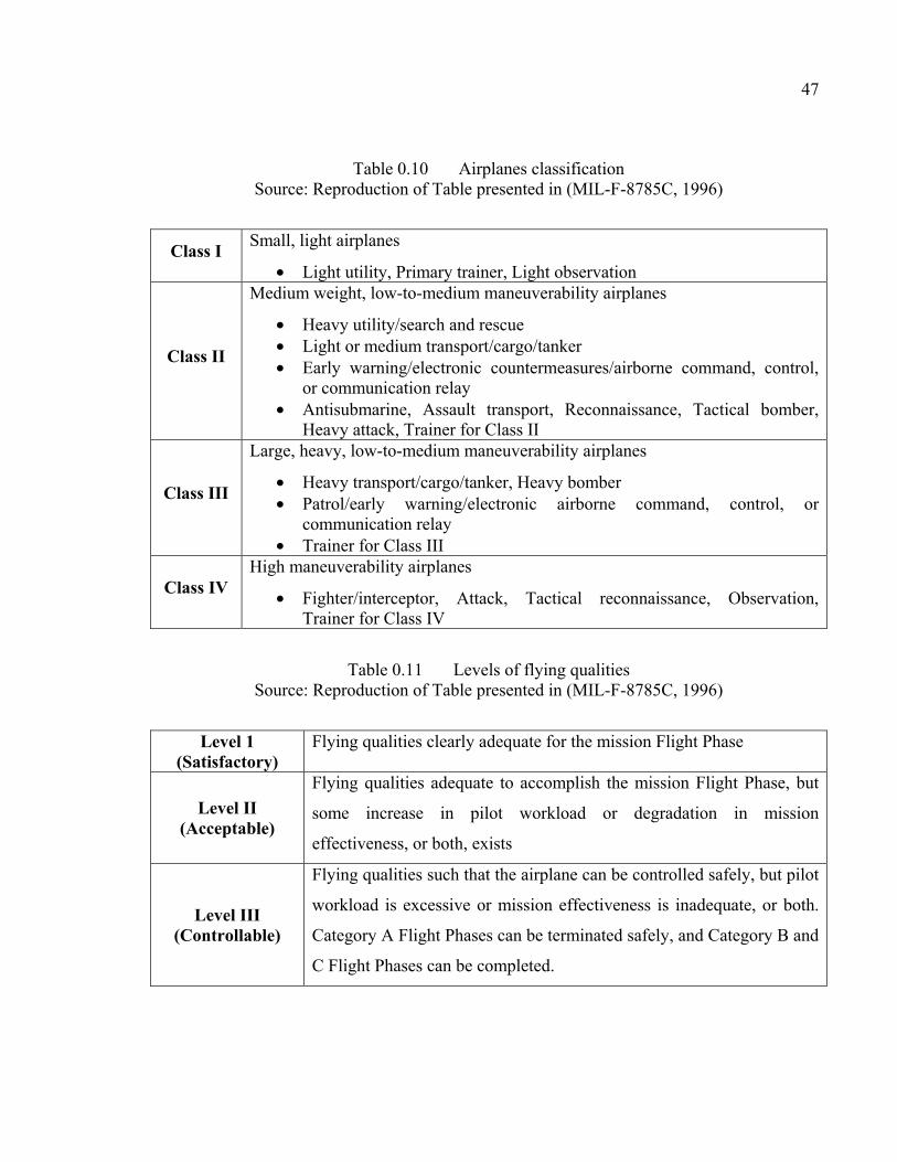
47

Table 0.10 Airplanes classification Source: Reproduction of Table presented in (MIL-F-8785C, 1996)

Class I Small, light airplanes

• Light utility, Primary trainer, Light observation

Class II

Medium weight, low-to-medium maneuverability airplanes

• Heavy utility/search and rescue • Light or medium transport/cargo/tanker • Early warning/electronic countermeasures/airborne command, control,

or communication relay • Antisubmarine, Assault transport, Reconnaissance, Tactical bomber,

Heavy attack, Trainer for Class II

Class III

Large, heavy, low-to-medium maneuverability airplanes

• Heavy transport/cargo/tanker, Heavy bomber • Patrol/early warning/electronic airborne command, control, or

communication relay • Trainer for Class III

Class IV High maneuverability airplanes

• Fighter/interceptor, Attack, Tactical reconnaissance, Observation, Trainer for Class IV

Table 0.11 Levels of flying qualities Source: Reproduction of Table presented in (MIL-F-8785C, 1996)

Level 1 (Satisfactory)

Flying qualities clearly adequate for the mission Flight Phase

Level II (Acceptable)

Flying qualities adequate to accomplish the mission Flight Phase, but

some increase in pilot workload or degradation in mission

effectiveness, or both, exists

Level III (Controllable)

Flying qualities such that the airplane can be controlled safely, but pilot

workload is excessive or mission effectiveness is inadequate, or both.

Category A Flight Phases can be terminated safely, and Category B and

C Flight Phases can be completed.

48

Table 0.12 Flight phase categories Source: Reproduction of Table presented in (MIL-F-8785C, 1996)

Non-terminal Flight Phase

Category A

Require rapid maneuvering, precision tracking, or precise flight

path control

Air-to-air combat (CO) Ground attack (GA) Weapon delivery/launch (WD) Aerial recovery (AR) Reconnaissance (RC) In-flight refuelling (receiver) (RR) Terrain following (TF) Antisubmarine search (AS) Close formation flying (FF)

Category B

Normally accomplished using gradual maneuvers and without

precision tracking, although accurate flight path control may be

required

Climb (CL) Cruise (CR) Loiter (LO) In-flight refuelling (tanker) (RT) Descent (D) Emergency descent (ED) Emergency deceleration (DE) Aerial delivery (AD)

Terminal Flight Phase

Category C

Normally accomplished using gradual maneuvers and usually

requires accurate flight path control

Take-off (TO) Catapult take-off (CT) Approach (PA) Wave-off/go-around (WO) Landing (L)

The decision route used by flight-tests engineers and pilots to turn qualitative opinions of

aircraft performance into a quantitative rating is provided by the Cooper-Harper rating scale,

as illustrated in Figure 0.16 (Botez, 2004), (Hodgkinson, 1999), (Hahn et al., 1981).

49

Figure 0.16 Cooper-Harper rating scale

H. Root Locus method

The Root Locus method developed by Walter R. Evans to determine the stability of a system

is in fact a graphical method which examines how the roots of a system change with the

variation of certain system parameters. This method was applied here for longitudinal and

lateral dynamic analysis of the three types of aircraft.

The five modes of an aircraft are: the short period and the long period for longitudinal motion

and the roll, Dutch roll and spiral for lateral motion. The natural frequency (ωn) and the

50

damping ratio (ζ) are defined for each mode from the eigenvalues. For the longitudinal

stability analysis, two modes are studied: the short period and the phugoid. The short-term

pitch is a second order response. The phugoid mode is the long–term motion of an aircraft

after a disturbance.

The mathematical model of longitudinal dynamics is given in eq.(0.37) (Botez, 2004):

0

0,

0

0 0 1 0

, ,

0

u

qu

long

quu q

long long long e

X gX

V VV ZV Z Z

V Z V Z V Z

V ZV Z M Z MV M M M M

V Z V Z V Z

X

Vu

Z

V Z uq

Z MM

V Z

α

α

α α α

α α αα α

α α α

δ

δ

α

δ αδ

α

αδ

θ

−

+ − − −=

+ + + + − − −

Δ Δ −= = = Δ Δ +Δ −

A

x B

(0.37)

The roots of the characteristic equation det(λ I – Along) = 0 are used to determine the

eigenvalues λ1 to λ4. For both longitudinal modes, the natural frequency ωn and the damping

ratio ζ are estimated directly from the characteristic equation 0=− longAIλ , as a function of

the longitudinal eigenvalues (eq.(0.38)); the eigenvalues λ1,2 correspond to short-period and

λ3,4 to phugoid modes.

( )

( )( )

( )1,2 3,4

2 21,2 3,4

Re Re,

1 Im 1 Im

n n

n n

ςω λ ςω λ

ω ς λ ω ς λ

= =

− = − =

(0.38)

The matrices of the aircraft lateral model are defined in eq.(0.39) (Botez, 2004).

51

00

cos

0,

0

0 1 0 0

,

p r

x z x z x zp p r r

x x xlat

x z x z x zp p r r

z z z

x z

lat lat

YY Y V g

V V V u

I I IG L N G L N G L N

I I I

I I IG N L G N L G N L

I I I

Y

VI

G L Np

r

β

β β

β β

δ

δ δ

θ

β

φ

− + + + =

+ + +

Δ +Δ = = Δ Δ

A

x B ,

0

x lat a

x z

z

I u

IG N L

Iδ δ

δ

= Δ + (0.39)

Three modes are considered in the aircraft lateral motion modelling:

• Spiral mode, representing a convergent or a divergent motion;

• Roll mode, representing a fast convergent motion, and

• Dutch roll mode, representing a lightly-damped oscillatory motion with a low

frequency.

These modes are significant factors, mainly in the uniform cruise flight. For the lateral

aircraft motion modeling, two real roots correspond to the roll and spiral modes, and a pair of

complex roots correspond to the Dutch roll mode, obtained from the characteristic equation

0=− latAIλ .

The rolling motion is generally quite damped, and reaches the steady state in a very short

time. An unstable spiral mode results in a turning flight path. The Dutch roll is a nuisance

mode that appears in the basic roll response to lateral control that can induce uncontrolled

and undesired motions in roll and yaw modes. These motions have a serious impact on the

ability of the pilot to control lateral–directional motions with precision.

52

0.6 Continuity algorithm: application on High Incidence Research Model aircraft

This section presents the continuity algorithm (Hacker, 1992) and its application on the

HIRM aircraft for longitudinal motion. For a better grasp of this procedure, a graphical

scheme is very helpful; Fig. 0.17 shows the continuity algorithm broken into steps .

Figure 0.17 Steps of the continuity algorithm

Longitudinal model equation

of the aircraft (nonlinear

system) (eq.(5.9))

For the aircraft studied in this

paper, the aerodynamics

coefficients are CN, CT, CM = f (V,

α, δe) and the thrust T = f (V, δT)

Airspeed (or Mach number)

selected as parameter of continuity

With the H and V constants (defined in the flight envelope) we calculated

the initial condition for continuity algorithm, based on eq. (5.9)

N linear equations with N +1 unknowns ( , , ,e T Vα δ ) are solved based on

• Gaussian elimination with total pivoting, and

• The Adams-Bashforth method

The minimum airspeeds calculated above will define

the flight envelope

53

The continuity algorithm is applied in this thesis for longitudinal dynamics modeling of a

High Incidence Research Model (HIRM) aircraft implemented on the Aero-Data Model In

Research Environment (ADMIRE) model developed by the Swedish Defense Research

Agency FOI (Sweden), based on the Generic Aerodata Model (GAM) developed by SAAB

AB in the framework of the GARTEUR Group: « The ADMIRE describes a generic small-

single seated, single-engine fighter aircraft with a delta-canard configuration, implemented in

MATLAB/SIMULINK Release 13 » (Lars et al., 2005, p iii].

The HIRM of a generic fighter aircraft was used in this study ((Admirer4p1), (Lars et al.,

2005), (Terlouw et al., 1996)). Its flight envelope is presented in Figure 0.18 and its shape

shows how this model was chosen for the continuity algorithm. In the minimum airspeeds

range this envelope can be improved, stabilized with control laws.

Figure 0.18 Flight envelope of the HIRM aircraft Source: Reproduction of Figure presented by Lars et al., (2005)

The aerodynamics coefficients were obtained based on wind tunnel and flight tests

(Admirer4p1) for a model « ... originally designed to investigate flight at high angles of

54

attack ... but [that] does not include compressibility effects resulting from high subsonic

speeds. » (Terlouw et al., 1996, p 21). These coefficients were further implemented in the

ADMIRE model using the main graphical window simulation presented in Figure 0.19,

which also shows the response of the aircraft model. The tests and analyses provided in the

GARTEUR program were focused on PIO detection, while this paper evaluates a new

method to investigate the model’s stability.

« The ADMIRE contains twelve states (VT, α, β, pb, qb, rb, ψ, θ, φ, xv, yv, zv) plus additional states due to actuators and [the] Flight Control System (FCS). Available control effectors are left- and right canard, leading edge flap, four elevons, rudder and throttle setting. The model is also equipped with thrust vectoring capability and an extendable landing gear. The model is prepared for the use of atmospheric turbulence as external disturbance. The ADMIRE is augmented with an FCS in order to provide stability and sufficient handling qualities within the operational envelope (altitude <6 km, Mach < 1.2). The FCS contains a longitudinal and a lateral part. (...) The lateral controller enables the pilot to perform roll control where the roll motion is initiated around the velocity vector of the a/c, and [at the] angle of sideslip control. Sensor models are incorporated. The 20 ms flight computer delay on the actuator inputs that is implemented in other versions of ADMIRE was not used here. The model has the facility to define model uncertainties, but this was not used. ADMIRE is implemented in MATLAB and SIMULINK using a combination of standard SIMULINK blocks and S-functions written in C. » (GARTEUR FM(AG12), 2001, p 36).

55

Figure 0.19 ADMIRE: Main graphical window simulation and the aircraft response Source: Screenshot from Admirer4p1 interface

56

I. Mathematical model of the continuity algorithm

Let us consider that the system dynamics is expressed by the following autonomous non-

linear equation (Hacker, 1992):

( ),x f x u= (0.40)

with the output ( ),y g x u= . We assume that dim dimy u= . When a transition from one

regime to another is performed, the constant command value u must be determined. This

command corresponds to a steady state; its attraction area contains the initial state and the

output has the required steady state y , with the condition that the permanent regime is located

in an allowed given area. A continuous motion, given by a constant command u, described by

a stationary solution of the studied system, satisfies the nonlinear system of eq.(0.41)

( ), 0f x u = (0.41)

If required output value is defined as ˆ constanty y= = , a corresponding command will be

given by one of the values of u that satisfies the system equations with (n+p) unknowns (x

and u).

( )ˆ, , 0F x u y = (0.42)

If the matrix ( )ˆ ˆ,f

x ux

∂∂

is a Hurwitz matrix (i.e., all eigenvalues have negative real parts), the

asymptotic stability of the point x is ensured. Obtaining the desired regime depends, in

general, on the initial regime; it does not depend on the starting point from where the

command u is applied.

Assume that the airplane is in its flight mode corresponding to the stationary point

x0, the command u0 and the output 0y , so that f(x0, u0) = 0. x0 is stable and ( )0 0,f

x ux

∂∂

is a

57

Hurwitz matrix, with ( )0 0det , 0f

x ux

∂ ≠∂

. Then, the implicit function theorem can be applied;

in this theorem a function x is defined in the neighborhood of u0, with values in the vicinity

of x0, with ( )0 0 0x u x= and ( ) , 0f x u u ≡ through (x0, u0).

A path is considered, which connects u0 to u without leaving the area where ( ) ,f

x u ux

∂ ∂

remains a Hurwitz matrix; the command changes the value u0 into a value u1 that corresponds

to the regime ( )1x u , neighbor to x0. That point x0 is close to ( )1x u and is within its attraction

field after a short phase, so that we can consider that the state ( )1x u is reached. The

command then changes to the neighbor value u2 to reach the state ( )2x u and the process

continues in the same manner until a stable, steady branch of the stationary regime past state

x is reached.

Any asymptotically stable steady state x can be achieved based on other stable steady state x0

values, if there is at least one branch of a stable stationary regime with acceptable values («

allowed ») which link them together.

The equilibrium points defined as pairs of (α, δe, T) at a constant Mach number and altitude

for the HIRM model stabilized with control laws are defined based on system eq.(0.43). They

are subsequently used in the continuity algorithm by integration of the same system

equations.

J. Application on the longitudinal motion of the HIRM aircraft

The longitudinal system of equations (Lars et al., 2005) is given by eq.(0.43)

58

( )

( )

[ ]

1cos sin

1 1sin cos

1

D

L

m CG T ey

V qSC T gm

qSC T gmV V

q qScC x qSC z TI

q

α γ

γ α γ

α

= − − − = + −

= + + =

(0.43)

for which the altitude H is constant and the output is defined in the range of [Vmin, Vmax]. The

system variables are ( ), , andV qγ α with a command defined by ( ),e Tδ δ . The aim is to find

the values of (α, δe and T) of the nonlinear system's solutions found by using

cos sin 0

sin cos 0

0

D

L

m CG T e

qSC T mg

qSC T mg

qScC x qSC z T

α γα γ

− + = + − = + + =

(0.44)

based on the equilibrium points.

If conditions such as γ =const. and 0cδ = are imposed, the equation system of eq.(0.44) can

also be written as:

cos 0sin cos

sin 0 , where cos sin

0

DD N T

LL N T

m CG T e

qSC TC C C

qSC T mgC C C

qScC x qSC z T

αα α

αα α

− == + + − = = − + + =

(0.45)

The thrust is calculated using eq. (0.46).

cos

DqSCT

α=

(0.46)

The following combinations of altitude and Mach number were chosen from the flight

envelope: case 1 (20 m, 0.22), case 2 (3,000 m, 0.22) and case 3 (6,000 m. 0.55). The control

law is defined as δe = δe0 + kαα + kqq, where the regulator gains are known from the model

implemented in ADMIRE simulation (Admirer4p1). Based on the system of eq.(0.45), for all

three study cases the points of equilibrium (or the critical points) and the gain values are

59

presented in Table 0.15. For each combination of altitude and airspeed the aerodynamic

coefficients are known.

Table 0.13 Points of equilibrium; initial conditions of continuity algorithm

Case 1 Case 2 Case 3

Altitude H = 20 m H = 3000 m H = 6000 m

Mach number (M) 0.22 0.22 0.55

Angle of attack (α0) 9.5537 deg 13.0627 deg 3.5522 deg

Elevon angle (δe0) 3 deg 5 deg 0 deg

Thrust (T) 13683.47 N 18654.87 N 8481.61 N

kα 0.4321 0.4630 0.4574

kq 1.5729 0.8810 0.4693

Based on the differentiation method with respect to a parameter z(α) proposed by Davidenko

(1953), the following eq.(0.47) is considered:

( )( ), 0F z α α = (0.47)

where the solution is given as z(α0) = z0.

Because the aerodynamic coefficients CN, CT and CM depend on (V, α and δe) and the thrust

T is a function of (V and δT), the airspeed (or Mach number) was chosen to be a parameter of

the continuity algorithm.

We can now define all of the functions of the continuity algorithm for γ = 0 (see eq.(0.48))

( )( )( )

1 cos

2 sin

3

D

L

m CG T e

F qSC T

F qSC T mg

F qScC x qSC z T

αα

= −

= + −

= + +

(0.48)

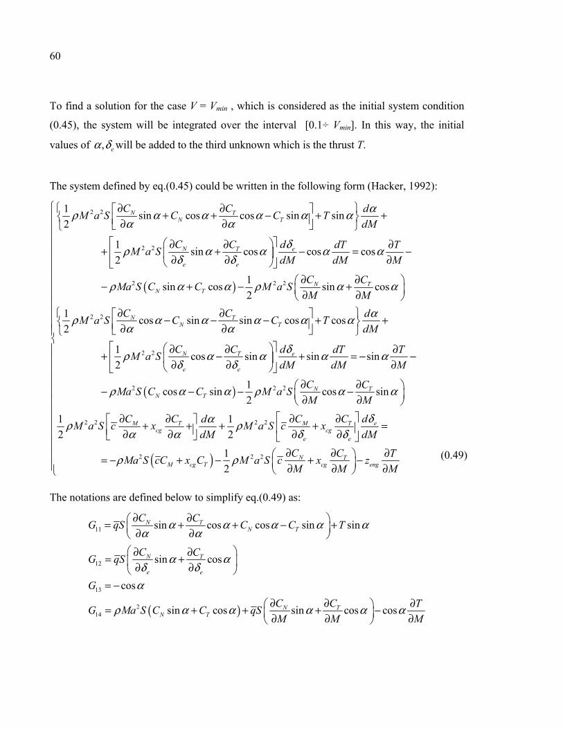
60

To find a solution for the case V = Vmin , which is considered as the initial system condition

(0.45), the system will be integrated over the interval [0.1÷ Vmin]. In this way, the initial

values of , eα δ will be added to the third unknown which is the thrust T.

The system defined by eq.(0.45) could be written in the following form (Hacker, 1992):

( )

2 2

2 2

2 2 2

2 2

1sin cos cos sin sin

2

1sin cos cos cos

2

1sin cos sin cos

2

1cos

2

N TN T

N eT

e e

N TN T

N

C C dM a S C C T

dM

C dC dT TM a S

dM dM M

C CMa S C C M a S

M M

CM a S

αρ α α α α αα α

δρ α α α αδ δ

ρ α α ρ α α

ρ αα

∂ ∂ + + − + + ∂ ∂ ∂ ∂ ∂+ + − = − ∂ ∂ ∂

∂ ∂ − + − + ∂ ∂ ∂∂

( )

2 2

2 2 2

2 2

sin sin cos cos

1cos sin sin sin

2

1cos sin cos sin

2

1

2

TN T

N eT

e e

N TN T

M Tcg

C dC C T

dM

C dC dT TM a S

dM dM M

C CMa S C C M a S

M M

C C dM a S c x

d

αα α α αα

δρ α α α αδ δ

ρ α α ρ α α

αρα α

∂ − − − + + ∂ ∂ ∂ ∂+ − + = − − ∂ ∂ ∂

∂ ∂ − − − − ∂ ∂

∂ ∂ + + ∂ ∂

( )

2 2

2 2 2

1

2

1

2

eM Tcg

e e

N TM cg T cg eng

dC CM a S c x

M dM

C C TMa S cC x C M a S c x z

M M M

δρδ δ

ρ ρ

∂ ∂ + + = ∂ ∂

∂ ∂ ∂ = − + − + − ∂ ∂ ∂ (0.49)

The notations are defined below to simplify eq.(0.49) as:

( )

11

12

13

214

sin cos cos sin sin

sin cos

cos

sin cos sin cos cos

N TN T

N T

e e

N TN T

C CG qS C C T

C CG qS

G

C C TG Ma S C C qS

M M M

α α α α αα α

α αδ δ

α

ρ α α α α α

∂ ∂ = + + − + ∂ ∂ ∂ ∂= + ∂ ∂

= −∂ ∂ ∂ = + + + − ∂ ∂ ∂

61

( )

21

22

23

224

cos sin sin cos cos

cos sin

sin

cos sin cos sin sin

N TN T

N T

e e

N TN T

C CG qS C C T

C CG qS

G

C C TG Ma S C C qS

M M M

α α α α αα α

α αδ δ

α

ρ α α α α α

∂ ∂ = − − − + ∂ ∂ ∂ ∂= − ∂ ∂

=∂ ∂ ∂ = − + − + ∂ ∂ ∂

(0.50)

( )

31

32

33

234

cos

cos

M Tcg

M Tcg

e e

eng

M TM cg T cg eng

C CG qS c x

C CG qS c x

G z

C C TG Ma S cC x C qS c x z

M M M

αα α

αδ δ

ρ

∂ ∂ = + ∂ ∂ ∂ ∂= + ∂ ∂

=

∂ ∂ ∂ = + + + + ∂ ∂ ∂

The following eq.(0.51) is equivalent with eq.(0.49) and (0.50):

11 12 13 14

21 22 23 24

31 32 33 34

e

e

e

dd dTG G G G

dM dM dMdd dT

G G G GdM dM dM

dd TG G G G

dM dM M

δα

δα

δα

+ + = + + =

∂ + + = − ∂

(0.51)

The following algorithm allows N linear equations with N +1 unknowns ( , , ,e T Vα δ ) to be

solved, based on Gaussian elimination with total pivoting (Olson, 2006)] and the Adams-

Bashforth method (Hoffman, 2001). The Gaussian algorithm with total pivoting is

performed in two steps:

• forward elimination when a matrix is transformed into an upper triangular equivalent

matrix; and

• backward substitution.

62

The pivot element is chosen as the greatest element, in absolute value, between the elements

that are found in the upper triangular equivalent matrix; once the greatest element is

identified, an interchange is performed between the rows and columns.

The Adams-Bashforth method is an explicit linear multistep method that depends on multiple

previous solution points for solving initial value problems for ordinary differential equations.

It is a numerical method to solve an ordinary differential equation (ODE) to obtain an

approximate solution, step-by-step in discrete increments across the interval of integration.

The system of eq.(0.51) is integrated with initial conditions defined as points of equilibrium,

and the minimum airspeed is calculated using the principle presented before. Starting from

the initial pair of equilibrium points, a new asymptotically stable steady state is found at each

integration step and a branch of the stable stationary regime is defined.

The range variation of Mach number is M = [Mmin÷0.22], for H = 20 m, 3,000 m M =

[Mmin÷0.55] for H = 6,000 m with angle of attack α = [-10÷30]0 and elevon angle δe = [-

30÷30]0. The results are presented in Figures 0.20 to 0.22 for each case studied, for angle of

attack α, elevon angle δe and thrust T versus airspeed V.

63

64

Figure 0.20 Angle of attack, elevon angle and thrust variation versus airspeed V, starting at the initial conditions presented in Table 5.4 for H = 20 m

and M = 0.22

65

66


and M = 0.22

67

68


and M = 0.55

All three minimum airspeeds for the initial conditions (α, δe and T) presented in Table 0.13

have been determined, such as Vcase1 = 62.09 m/s, Vcase2 = 63.15 m/s, and Vcase3 = 111.8 m/s.

The new flight envelope for HIRM aircraft stabilized with control laws is presented in Figure

0.23.

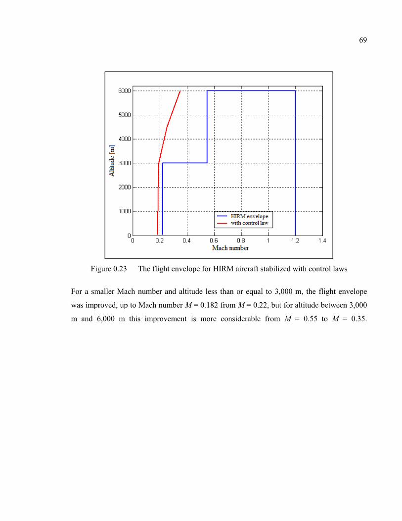
69

Figure 0.23 The flight envelope for HIRM aircraft stabilized with control laws

For a smaller Mach number and altitude less than or equal to 3,000 m, the flight envelope

was improved, up to Mach number M = 0.182 from M = 0.22, but for altitude between 3,000

m and 6,000 m this improvement is more considerable from M = 0.55 to M = 0.35.

The literature review is explained in different sections. The first section presents the

bibliographical research on the semi–analytical techniques needed to calculate stability

derivatives from aircraft geometry using parameter estimation methods. The theory of the

Computational Fluid Dynamics method required for the calculation of aerodynamics

coefficients and their derivatives is presented in the second section, and the weight functions

method review is in the third. Independent codes have been developed based on the

DATCOM or vortex methods.

1.1 Methods used by semi-empirical codes to calculate the aerodynamics coefficients and their stability derivatives

The aerodynamic coefficients and their stability derivatives based on the DATCOM method

have been estimated in the literature. Some methods were adapted directly from the original

method and others combined DATCOM with the vortex–lattice method. Grasmeyer (1998)

has estimated the stability and control derivatives of Boeing 747–100 aircraft using a method

adapted from the USAF Stability and Control DATCOM (Williams et al., 1979a).

MacMillin (1996) has used a similar approach for the High–Speed Civil Transport (HSCT).

The baseline stability and control derivatives were estimated using the vortex–lattice method,

and then the DATCOM method was used to increase these baseline values with the effects

due to vertical tail geometry changes.

A computer code for calculating the dynamic stability derivatives of an airplane from static

wind tunnel tests was developed by Chang et al. (2004). This methodology was mainly based

on the DATCOM method, but the wing and tail static coefficients were obtained from

breakdowns of body, wing–body, and tail–body tests instead of from direct tests of each

CHAPTER 1

LITERATURE REVIEW

72

component. Evaluation of the code was carried out for a Standard Dynamic Model of a twin

prop airplane. The results of this code were better than results achieved with DATCOM.

1.1.A Digital DATCOM (DATCOM+) code description

Digital DATCOM code (Galbraith), also known as DATCOM+, is the first implementation

of the DATCOM procedures in an automatic calculation code. The software is a portable

application, directly executable. Input data, consisting of geometric and aerodynamic

parameters of the aircraft and flight conditions, are introduced through a text file called «

aircraft_name.dcm » whose format is specific to the software. The input format of Digital

DATCOM is a series of NAMELIST statements. The data entry file can contain more than

300 variables for a complete aircraft configuration.

The DATCOM+ program calculates the static stability, the high lift and control, and the

dynamic derivative characteristics. This program applies to aircraft flying in the subsonic,

transonic and supersonic regimes, more precisely to traditional wing-body-tail and canard-

equipped aircraft. DATCOM+ offers a trim option that computes the control deflections and

aerodynamic data needed to trim the aircraft in the subsonic Mach regimes. The program has

a modular basis with 3 master routines:

Main programs

Perform the executive functions of organizing and

directing the operations performed by other program

components.

Executive subroutines Perform user–oriented non-method operations such as

ordering input data, switching logic, input error analysis,

and output format selection.

Utility subroutines Perform mathematical tasks repetitively, using

subroutines.

Module 1/ Module 3 / Module 5 Contain the coefficients at the angle of attack for the

subsonic, transonic, and supersonic regime (CD, CL, Cm,

73

CN, CLα, and Cmα).

Module 2 / Module 4 / Module 6

Contain the coefficients at the sideslip angle for the

subsonic, transonic, supersonic regime (Cyβ, Cnβ, and

Clβ).

Module 7

Gives the low-aspect wing-body ratio at subsonic speeds

for different configurations, with a trim option.

Module 8

Provides aerodynamic control effectiveness at

hypersonic speeds for special configurations. A special

configuration means the low aspect ratio wing or wing-

body configurations (lifting bodies) are treated in

subsonic regimes, and the two-dimensional flap and

transverse jet effects are treated in hypersonic regimes.

Module 9

Provides traverse-jet control effectiveness at hypersonic

speeds for special configurations.

Module 10

Gives the dynamic derivatives at the subsonic, transonic,

and supersonic regimes (CLq, Cmq, , ,Clp, Cyp, Cnp,

Cnr, Clr).

Module 11

Acts as a high lift and control device for subsonic,

transonic, supersonic regimes.

Once the airplane’s geometry is defined, the outputs can be obtained rapidly; their accuracy

depends mainly on the accuracy of the inputs. Despite its drawbacks, there remains

significant interest in the Digital DATCOM code in the aviation field.

For an input file called aircraft_name.dcm, the outputs of DATCOM+ are given in the

following formats:

• aircraft_name.out – contains values of the inputs defined in aircraft_name.dcm. For

each section of wing, horizontal tail, vertical tail and canard (if it exists), the

following 11 parameters are estimated.

74

Ideal angle of attack = value (deg)

Zero lift angle of attack = value (deg)

Ideal lift coefficient = value

Zero lift pitching moment coefficient = value

Mach zero lift-curve-slope = Value (1/deg)

Leading Edge radius = value (Chord fraction)

Maximum airfoil thickness = value (Chord fraction)

Delta-y = value (Percent chord)

Mach = value

Lift-curve-slope = value (1/deg)

xAC = value

Complete aircraft configuration results are presented in Table 1.1, as functions of the flight

conditions and reference dimensions.

Table 1.1 Outputs of Digital DATCOM code

------------------------------------------------ FLIGHT CONDITIONS ----------------------------------------------------- MACH_NUMBER ALTITUDE VELOCITY PRESSURE TEMPERATURE REYNOLD_NUMBER FT FT/SEC LB/FT2 DEG R 1/FT ---------------------------------------------- REFERENCE DIMENSIONS ------------------------------------------------- REF._AREA REFERENCE_LONG. LENGTH_LAT. MOMENT_REF._HORIZ. CENTER_VERT FT2 FT FT FT FT ---------------------------------------------DERIVATIVE (PER RADIAN) ------------------------------------------------ ALPHA CD CL CM CN CA XCP CLA CMA CYB CNB CLB

ALPHA Q/QINF EPSLON D(EPSLON)/D(ALPHA)

----------------------------------------- DYNAMIC DERIVATIVES (PER RADIAN) ---------------------------------- -----PITCHING---- ---ACCELERATION--- ---------ROLLING---------- ------YAWING----- ALPHA CLQ CMQ CLAD CMAD CLP CYP CNP CNR CLR

BASIC BODY PROPERTIES WETTED

AREA

XCG ZCG BASE

AREA

ZERO LIFT

DRAG

BASE

DRAG

FRICTION

DRAG

PRESSURE

DRAG

XCG RELATIVE TO THEORETICAL LEADING EDGE MAC

75

BASIC PLANFORM PROPERTIES

AREA TAPER

RATIO

ASPECT

RATIO

QUARTER

CHORD

SWEEP

MAC QUARTER

CHORD

X(MAC)

Y(MAC) ZERO

LIFT

DRAG

FRICTION

COEFFICIENT

Estimated for:

• Wing - total theoretical and total exposed

• Horizontal Tail - total theoretical and total exposed

• Vertical Tail - total theoretical and total exposed

CHARACTERISTICS OF HIGH LIFT AND CONTROL DEVICES TAIL PLAIN TRAILING-EDGE

FLAP CONFIGURATION

--------INCREMENTS DUE TO DEFLECTION------ ---DERIVATIVES (PER DEGREE)---

DELTA D(CL) D(CM) D(CL MAX) D(CD MIN) (CLA)D (CH)A (CH)D

--------- INDUCED DRAG COEFFICIENT INCREMENT , D(CDI) , DUE TO DEFLECTION ---------

For each delta(trailing-edge flap, in this case) as function of angle of attack α

CHARACTERISTICS OF HIGH LIFT AND CONTROL DEVICES WING-BODY-TAIL TRIM WITH

CONTROL DEVICE ON TAIL

----UNTRIMMED--- --------------------------AT TRIM DEFLECTION----------------------------------

ALPHA CL CD CM DELTAT D(CL) D(CL MAX) D(CDI) D(CD MIN) CH(A) CH(D)

• aircraft_name.ac – shows the 3D aircraft visualization

76

Figure 1.1 3D aircraft’s visualization in Digital DATCOM code

• aircraft_name.xml – generates a folder called aircraft_name.jiff which contains

images with extension .png for all outputs computed with Digital DATCOM code.

Figure 1.2 Drag coefficient due to elevator deflection results obtained with aircraft_name.xml command for A-380 aircraft, presented in the example given by Digital

DATCOM code

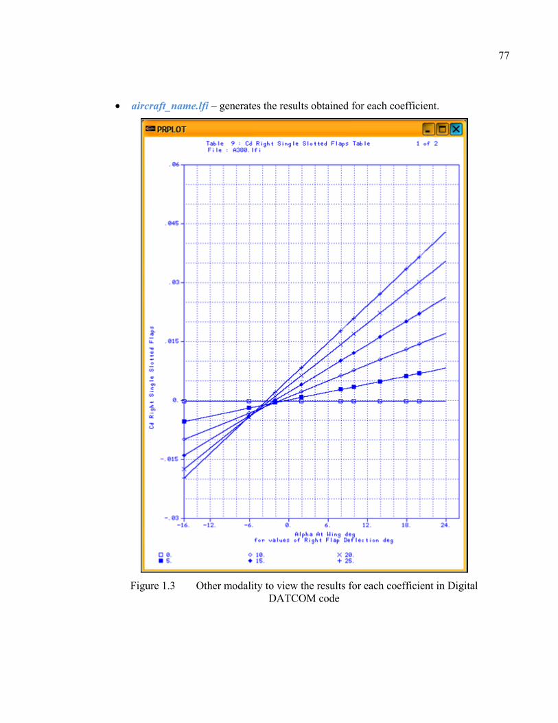
77

• aircraft_name.lfi – generates the results obtained for each coefficient.

Figure 1.3 Other modality to view the results for each coefficient in Digital DATCOM code

78

1.1.B Advanced Aircraft Analysis (AAA) code

ADVANCED AIRCRAFT ANALYSIS (AAA) (Advanced Aircraft Analysis 3.3 code) is a

code created by the Design, Analysis and Research Corporation (DARcorporation), an

American company. This code is a computational tool utilized in an iterative process for

preliminary aircraft design. AAA uses methodologies, statistical databases, formulas and

drawings described in the following books: Airplane Design (Roskam, 2000), Airplane Flight

Dynamics and Automatic Flight Controls (Roskam, 1995) and Airplane Aerodynamics and

Performance (Lan et al., 1981), . AAA is the industry standard aircraft design, stability and

control analysis code; it can be used for small civil, military and transport aircrafts. The

software has 10 independent modules, including one that estimates the aerodynamic

coefficients and stability derivatives for the subsonic regime. Other modules estimate the

weight, aerodynamics, performance, geometry, propulsion, stability and control, dynamics,

loads, structures, cost analysis, atmosphere and flight conditions.

1.1.C MISSILE code

The MISSILE code (Champigny et al., 2004) was developed by the National Office for

Studies and Research Aerospace (ONERA) in France to provide rapid estimations of

aerodynamic missiles’ characteristics, for Mach numbers up to 10, angles of attack up to 400,

angles of control surfaces of maximum ± 300 and different roll angles. The methodology used

in this code is based on the concept that the angle of incidence is equivalent to the

integration of vortex effects. It relies on semi–empirical theoretical methods and database

correlations. The MISSILE code uses DATCOM’s methods.

1.2 Computational Fluid Dynamics (CFD) methods

Another, more expensive method in terms of computational resources, and therefore in

calculation time, is the use of CFD methods, fundamentally based on the Navier–Stokes

equations. The steady (time–invariant) aerodynamic forces and moments are defined at

79

different flight conditions expressed in terms of Mach numbers and angles of attack

(Limache, 2000). This model required the extension of standard (inertial) CFD formulations

to non–inertial reference coordinates systems, in which the aerodynamic forces

corresponding to the steady flows around the moving aircraft are numerically calculated. The

advantage of a CFD method lies in the way in which the aerodynamic forces are defined as

functions of motion variables.

A low–order panel method code on a simplified F–16XL fighter configuration was presented

in Green et al., 2004, where the twist effects on the performance of a finite wing of arbitrary

shape were also determined. This approach was based on Prandtl’s classical lifting–line

theory, where the Fourier coefficients depended only on the wing geometry.

In (Phillips et al., 2006), the predicted results obtained with the new lifting–line method were

compared with the results predicted from computational fluid dynamics (CFD) solutions. In

every case, the CFD solutions showed that the drag reduction achieved with optimum twist

was equal to or greater than that predicted by the lifting–line method.

The CFD method predicted the maximum lift coefficient for a finite wing from knowledge of

the wing geometry and maximum lift coefficient for an airfoil section (Alley et al., 2007).

The method used a correlation obtained from grid–resolved CFD solutions for 25 different

wing geometries. These wings had aspect ratios ranging from 4 to 20, taper ratios from 0.5 to

1.0, quarter–chord sweep angles from 0 to 30 degrees, and linear geometric washout ranging

from 0 to 8 degrees. For these ranges of parameters, the ratio of maximum wing lift to

maximum airfoil section lift coefficients varied from about 0.70 to 0.98, with high aspect

ratio tapered wings producing the highest lift coefficient values and low aspect ratio wings

with washout and sweep producing the lowest lift coefficient values.

A novel CFD method of calculating dynamic stability derivatives was presented in Murman,

(2005). This method used a non–linear reduced–frequency approach to simulate the response

to a forced oscillation using a single frequency component at the forcing frequency. The

80

reduced–frequency approach was implemented using an automated Cartesian mesh scheme.

This combination of Cartesian meshing and a reduced–frequency solver enables damping

derivatives for arbitrary flight condition and geometric complexity to be efficiently and

accurately calculated. The method was validated for 3D reference missile and aircraft

dynamic test configurations during transonic and high–alpha flight regimes.

Babcock and Arena (2004) developed a CFD method for the determination of rate dependent

aerospace vehicle stability derivatives based on finite element analysis. This method

implemented an Euler routine capable of solving flow equations in a non–inertial reference

frame. The non–inertial boundary condition equation of the flow solver was modified in

order to decouple the position and velocity boundary conditions. The decoupled boundary

condition method gave reliable results comparable to the results obtained by theoretical

equations, empirical methods, and experimental data over a range of Mach numbers and

geometric complexities, including results for the F–18 aircraft in the transonic regime.

1.3 Weight Functions Method

The Weight Functions Method (WFM) has been applied in various engineering fields. For

example, it has been used to determine stress factors for crack problems. The WFM was

applied by Yoichi et al. (2003) to solve two- and three-dimensional crack problems and to

calculate stress intensity factors for arbitrary loading conditions. Their application has been

generalized to calculate the response analysis of structures and to solve two-dimensional

elasticity and plate bending problems. The weight functions method was found to be useful

for analyzing structures subjected to a variety of loading conditions, since the responses

expressed in terms of displacements and stresses may be calculated by integrating the inner

product of a universal weight function and a load vector. The stress intensity factor for a

patched crack within an infinite plate was successfully numerically validated using the WFM

(Kim et al., 2000).

81

Paris et al. (1976) presented a method that is an alternate use of Bueckner and Rice’s

proposal (Rice, 1972) for the deviation of a two-dimensional weight function to eliminate

crack tip stress intensity factors. A generalized weight functions method was developed by

Wu et al. (1983) based on applying Maxwell-Betti's reciprocal theorem to the equivalent

cracks problem involving mixed boundary conditions. Fett (1991) contributed an analytical

solution for determining stress distribution using a weight function based on the Boundary

Collocation Method. Schneider et al. (1989) used a closed-form weight function formula to

calculate the stress intensity factor of an edge crack for an elastic disc. A three-dimensional

linear elastic fracture mechanics (LEFM) problem was also solved using the WFM

(Vainshtok et al., 1987).

Stroe (2008) solved the Lurie-Postnikov problem using general vibration equations involving

linear transformations. Stroe also analyzed a holonomic system with dependent variable

equations, where the WFM was applied to vibration and stability studies in cases of damped

holonomic systems (Stroe et al., 2008).

The selections of H∞ weighting functions were presented for practical applications by

Jiankun et al. (2000), where the authors showed that an H∞ weighting function for a single-

input single-output system could be obtained by considering it as a series of connections of

elementary low-order systems. For a constrained control effort, an explicit weighting

function was obtained. They proposed a novel method for the selection of weighting

functions in an H∞ mixed sensitivity design to directly control the percentage overshoot.

Real-time experimental results were presented for the roll-angle control of a laboratory scale

model of a vertical take-off aircraft (Jiankun et al., 2000).

1.4 Other methods in the literature

Bryson developed a technique to determine static and dynamic stability derivatives of in

slender bodies. The technique was based on the transformation of three-dimensional flow

problems into two-dimensional, incompressible flow problems applied on the cross section

82

perpendicular to the long axis of the body, and used the concept of apparent–mass

coefficients (Bryson, 1953).

An adaptive estimation method for determining unknown parameters in linear time invariant

state equations was presented (Nakamura et al., 2002). The system was described using

multiple observers for virtual systems with linear combinations. This method was applied to

estimate the stability derivatives for an aircraft and proved its usefulness. It utilizes the

subspace method with the coefficient matrices derived from input and output data to identify

the state space models.

A new parameter identification algorithm called the Modified–Gain Extended Kalman Filter

(MGEKF) was applied of an F–111 aircraft to solve the on-line state estimation and

identification of the stability derivatives (Speyer et al., 1987). The filter formulation included

a simplified Dryden wind gust model. The inclusion of the wind gust model resulted mainly

in a slow response in the estimation of the stability derivatives associated with the

acceleration state; estimates of the stability derivatives with the pitch rate were also

calculated.

Using the concepts of aerodynamic and structural influence coefficients, Roskam (1973) has

presented a method for estimating longitudinal stability derivatives for rigid and elastic

airplanes. The structure of the airplane was divided into a large number of surface panels.

The elastic properties of the airplane were represented by a flexibility influence coefficient

matrix. Matrix algebra was used to obtain explicit expressions for longitudinal stability

derivatives, with angles of attack α, speeds on the x-axis u, and pitch rates q. To validate this

method, comparisons were performed with wind tunnel data for angles of attack α– and

speeds on the z-axis w; derivatives obtained with a Boeing 707 model and with rigid and

elastic models of a variable sweep supersonic transport configuration. There was very good

agreement between the theory and tunnel data.

Vorstab95 (online source) is a computer program developed at Kansas University for aircraft

aerodynamic coefficients and stability derivatives predictions for any aircraft configuration.

This code uses the vortex method to predict stability derivatives at high angles of attack.

83

Vorstab95 calculates the lift, drag, side force, pitching moment, rolling moment, yawing

moment, hinge moment, torsional moment, bending moment, longitudinal stability

derivatives and lateral directional stability derivatives.

Nicoleta Anton, Ruxandra Mihaela Botez and Dumitru Popescu École de Technologie Supérieure, Montréal, Canada

Laboratory of Research in Active Controls, Aeroservoelasticity and Avionics This article was published in The Aeronautical Journal, Vol. 114, No. 1156,

June 2010, Paper No. 3454

Résumé

Le nouveau programme FDerivatives a été conçu et développé pour calculer des dérivées de

stabilité statiques et dynamiques d’un aéronef en régime subsonique, en se basant sur ses

données géométriques. Le code est robuste et utilise les données géométriques et les

conditions du vol pour calculer les dérivées de stabilité de l'avion. Le programme

FDerivatives contient des nouveaux algorithmes et des nouvelles méthodes qui ont été

ajoutés à la méthode classique DATCOM, présentée dans la référence « USAF Stability and

Control DATCOM ». Le nouveau code a été écrit en utilisant MATLAB et il possède une

structure complexe, qui contient une interface graphique pour faciliter le travail des

potentiels utilisateurs. Les résultats obtenus avec le nouveau code ont été évalués et validés

avec des données d'essais en vol prévus par CAE Inc. pour l’avion d'affaires Hawker 800XP.

Abstract

The new FDerivatives code was conceived and developed for calculating static and dynamic

stability derivatives of an aircraft in the subsonic regime, based on its geometrical data. The

code is robust and it uses geometries and flight conditions to calculate the aircraft’s stability

derivatives. FDerivatives contains new algorithms and methods that have been added to

DATCOM’s classical method, presented in a USAF Stability and Control DATCOM

reference. The new code was written using MATLAB and has a complex structure which

CHAPTER 2

ARTICLE 1: NEW METHODOLOGY AND CODE FOR HAWKER 800XP AIRCRAFT STABILITY DERIVATIVES

CALCULATIONS FROM GEOMETRICAL DATA

86

contains a graphical interface to facilitate the work of potential users. Results obtained with

the new code were evaluated and validated with flight test data provided by CAE Inc. for the

Hawker 800XP business aircraft.

2.1 Introduction

In this paper, we describe how we used and improved DATCOM procedures (Finck et al.,

1978) for the estimation of the semi–empirical aerodynamic coefficients and stability

derivatives, based on geometrical aircraft data. The main advantage of these procedures is

their collection of non–iterative faster methods – in terms of execution time – compared with

the numerical aerodynamic computational fluid dynamics methods used within the

aeronautical field.

Digital DATCOM (Galbraith) is the first implementation of the DATCOM procedures in an

automatic calculations code. Better estimation has been presented by Blake et al. (2005) for

the cambered fuselage pitching moment, compared to the one given in the DATCOM

procedures. In this new estimation, the equations using the thin airfoil theories for the

calculation were modified ((Williams et al., 1979a), (Williams et al., 1979b)). The results

obtained with this new estimation, expressed in terms of the cambered fuselage pitching

moment, were different for an asymmetric fuselage with respect to the DATCOM procedure,

but remained the same for the symmetric fuselage.

The ADVANCED AIRCRAFT ANALYSIS (AAA) is a code, created by the American

company Design, Analysis and Research Corporation (DARcorporation). This code is a

computational tool used in the iterative process for preliminary aircraft design, and uses

methodologies described in the Roskam (1973, 1995) and Roskam et al. (1997) books. This

code has 10 independent modules, including one which provides the estimation of

aerodynamic coefficients and stability derivatives for the subsonic regime (Advanced

Aircraft Analysis 3.3 code).

87

The MISSILE code (Champigny et al., 2004) was developed by ONERA, in France, for the

aerodynamic characteristics estimation of missiles at angles of attack up to 40°, for control

surfaces angles of ± 30° and at different rolling angles. The MISSILE and AAA codes use

the DATCOM methods.

The DATCOM procedures review allowed us to discover its lack of methods for the

calculation of the angle of attack at zero lift (α0) and the pitching moment coefficient at zero

lift (Cm0). Furthermore, the available methods in the procedures for the wing lift–curve slope

calculations have not taken into account the aerodynamic twist, the stall angle (αCLmax) and

the maximum lift–coefficient estimations. Almost all methods of DATCOM procedure,

concerning the fuselage aerodynamic, are applied to bodies of revolution.

Stability derivatives are considered to be part of an aircraft’s intrinsic parameters, as they are

dependent on its geometry and flight condition. A cost–effective way to reduce the necessary

amount of flight test data is to estimate the aircraft’s stability derivatives from its geometrical

data, by use of efficient numerical prediction methods.

In Section 2.2 a brief description of the classical DATCOM method is presented, followed by

the Hawker 800XP aircraft presentation given in Section 2.3.

The new FDerivatives code and its graphical interface (Section 2.4) does not only allow

designers to evaluate derivatives, but also to evaluate new aircraft design concepts, to predict

their performance, and to make modifications before performing more detailed design

evaluations.

This section also contains a logical description of the code. All of the parameters involved in

the stability derivatives estimation procedure are calculated with the new code for the

following three configurations: Wing alone (W), Wing – Body (WB), and Wing – Body –

Tail (WBT), from the essential geometrical data.

88

All improvements that were added to the DATCOM method (Popescu, 2009) are covered in

Section 2.5. For example, the wing lift–distribution method is improved, the drag coefficient

for WB configuration is calculated using a new nonlinear regression analysis, the longitudinal

dynamic stability coefficients CLq and Cmq are estimated by considering their dependence on

the dynamic–pressure ratio, and new functions are implemented for rolling–moment, side–

force and yawing–moment coefficients due to the time variation in the sideslip angle, for the

WBT configuration.

In Section 2.6, the stability derivatives obtained with FDerivatives are validated and

presented for various flight cases, expressed in terms of Mach numbers and altitudes, for

which experimental and geometrical Hawker 800XP aircraft data is available.

The aircraft data (geometrical and experimental) available in the literature is used for

validation of the FDerivatives code and methodologies for the W and WB configurations.

The flight test and geometrical data for the Hawker 800 XP were provided by CAE Inc. at

subsonic speeds and since their numerical values are confidential, they are not presented.

Results obtained with the FDerivatives code were validated at an altitude of 30 ft and a Mach

number between 0.2 and 0.6 for the WBT configuration of the Hawker 800 XP. For future

work, we are considering the validation of the stability derivatives obtained with

FDerivatives code for the WBT configuration of the Hawker 800 XP aircraft on a Cessna

Citation X research aircraft simulator at the LARCASE laboratory.

2.2 Brief description of the DATCOM method

The static and dynamic derivatives may be estimated from a knowledge of aircraft geometry

alone (Finck et al., 1979a), using the DATCOM method. The traditional WBT geometries,

including the control effectiveness for a variety of high–lift/control devices, are treated in the

USAF’s Stability and Control DATCOM program. The Digital DATCOM program written

in FORTRAN (Galbraith) is used to validate a number of stability derivatives obtained with

FDerivatives code, which are the ones described in the next two paragraphs.

89

• All of the static stability derivatives (longitudinal and the lateral–directional) are

expressed in the stability–axis system. The body–axis normal force and the axial–force

coefficients are also estimated. For various flight conditions, i.e. Mach numbers (speeds)

and angles of attack, and for all three configurations, the longitudinal drag, lift, moment,

normal and axial coefficients CD, CL, Cm, CN and CA and their corresponding lift, moment,

side–force, normal and roll derivatives with respect to the angle of attack and sideslip

angle CLα, Cmα, Cyβ, Cnβ and Clβ are obtained.

• The lift, moment, roll, side–force, and normal dynamic derivatives with respect to the

pitch, angle of attack, roll and yaw rates , , , , , ,Lq mq L m lp np nrC C C C C C Cα α& & and lrC are also

obtained. In the FDerivatives code, other functions available within the DATCOM

method are implemented for the calculation of drag, side force, normal and roll derivatives

with respect to the sideslip angle rate β& such as , ,D y nC C Cα β β& && and

lC β&.

2.3 Aircraft model

The Hawker 800XP is a midsize twin–engine corporate aircraft with low swept–back one–

piece wings, a high tailplane and rear–mounted engines, for which the maximum Mach

number is equal to 0.9. This aircraft operates in the subsonic and transonic regimes. Three

views of the Hawker 800XP aircraft are represented in the OXYZ reference system (Figure

2.1).

Figure 2.1 Three views of the Hawker 800XP aircraft

90

The most important geometrical characteristics of the Hawker aircraft, estimated from its

geometrical drawings and verified with other methods available in the literature, are found

for two different surfaces – fuselage and lift surfaces such as wing, horizontal tail and

vertical tail:

• The length and the position of the gravity centre for the body;

• The reference area, span, aspect ratio, Mean Aerodynamic Chord (MAC), thickness

ratio, leading–edge sweep (inboard/outboard), semi–span of exposed surface, root

chord, tip chord and MAC for the wing, horizontal tail and vertical tail surfaces.

2.4 FDerivatives’ new code

The new features (i.e. advantages) of the FDerivatives code, developed at the LARCASE

laboratory with respect to the Digital DATCOM code, are described next.

The principal main advantage of this new code is the estimation of the lift, drag and moment

coefficients and their corresponding stability derivatives by use of a select few aircraft

geometrical data: area, aspect ratio, taper ratio and sweepback angle for the wing and the

horizontal and vertical tails. In addition, the airfoils for wing, horizontal and vertical tail, as

well as the fuselage and nacelle parameters, are introduced in a three–dimensional plane.

The FDerivatives code was written on MATLAB and has a complex structure which contains

a graphical interface to facilitate the work of potential users. The code uses a total of 82

MATLAB functions; the aerodynamic coefficients and their stability derivatives are

calculated with 24 of these:

• 3 functions for estimation of the lift, drag and moment coefficients CL, CD and Cm;

• 6 functions for estimation of the static derivatives CLα, CDα, Cmα, Cyβ, Cnβ and Clβ;

• 15 functions for estimation of the dynamic derivatives:

i. 3 pitch rate (q) derivatives CLq, Cmq and CDq;

ii. 3 angle of attack rate ( Cα&) derivatives ,L mC Cα α& &and DC α&;

iii. 3 roll rate (p) derivatives Clp, Cnp and Cyp;

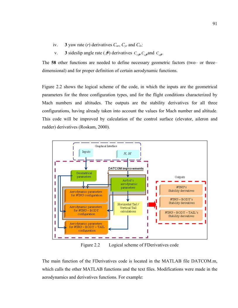
91

iv. 3 yaw rate (r) derivatives Cnr, Cyr and Clr;

v. 3 sideslip angle rate ( β&) derivatives ,Y n

C Cβ β& &and n

C β&.

The 58 other functions are needed to define necessary geometric factors (two– or three–

dimensional) and for proper definition of certain aerodynamic functions.

Figure 2.2 shows the logical scheme of the code, in which the inputs are the geometrical

parameters for the three configuration types, and for the flight conditions characterized by

Mach numbers and altitudes. The outputs are the stability derivatives for all three

configurations, having already taken into account the values for Mach number and altitude.

This code will be improved by calculation of the control surface (elevator, aileron and

rudder) derivatives (Roskam, 2000).

Figure 2.2 Logical scheme of FDerivatives code

The main function of the FDerivatives code is located in the MATLAB file DATCOM.m,

which calls the other MATLAB functions and the text files. Modifications were made in the

aerodynamics and derivatives functions. For example:

92

• The wing lift–distribution is calculated using the method presented by Sivells et al.

(1947) and Phillips et al. (2007). In this paper it is assumed that airfoil section

characteristics are not constant across the airfoil span;

• For WB configuration, the drag coefficient is calculated using a new nonlinear regression

analysis and the pitching moment was improved ((Multhopp, 1942), (Etkin et al., 1996));

• The longitudinal dynamic stability coefficients CLq and Cmq are estimated by considering

their dependence on the dynamic–pressure ratio;

• The new functions were implemented for rolling–moment, side–force and yawing–

moment coefficients due to a time variation in the sideslip angle, for WBT configuration.

The primary functions for the aircraft and airfoils’ geometry estimation are

aircraft_geometry.m, which has the global aim to determine the Wing, Horizontal/Vertical

Tail, Body and Nacelles geometries, while the function airfoil_properties.m is used to define

the geometrical and aerodynamic characteristics of different airfoils (two–/three–

dimensional).

The zero–lift angle and pitching moment for a wing section are calculated using the thin

wing section theory (Abbot et al., 1959). The details are presented in the section 0.4.

The graphical interface for the stability derivatives calculations (Figure 2.3) allows users to

make changes easily and rapidly in the aircraft geometrical data, and to choose different

flight conditions. For the same aircraft configuration, it will be possible to change only the

airfoil’s geometries.

93

Figure 2.3 Graphical interface of the FDerivatives code

In the main window, called Stability Derivatives, the platform’s (wing) type, configuration,

flight conditions (Mach numbers, altitudes and angles of attack ranges) are defined. It is

possible to fix the wing position and its roughness. For each of the three major components

(Wing, Horizontal/Vertical Tail), global parameters and airfoil coordinates situated at the

root, MAC and tip sections are considered. The Horizontal stabilizer may be positioned on

the fuselage or on the Vertical stabilizer. The inputs to the body configuration are the three

global parameters: body length, position of the gravitational centre and the fuselage

coordinates (in three dimensions) relative to the reference system (Figure 2.4). The positions

of the nacelles are described by their number, axial positions, lengths and coordinates relative

to the reference system.

94

Figure 2.4 Fuselage represented as a body of revolution

The outputs of the FDerivatives code are saved in three formats: jpeg, MATLAB figures, and

text files, which contain all of the numerical data.

2.5 DATCOM improvements for stability derivatives calculations

In the new FDerivatives code, it has implemented an additional number of derivatives,

calculated with DATCOM methods, which are not implemented in the Digital DATCOM

code. In addition, the method for lift–coefficient estimation has also been improved, and lift–

coefficient values were found that are closer to the experimental values than are Digital

DATCOM values. Table 2.1 shows all of the improvements associated with the FDerivatives

code.

Table 2.1 Outputs for Wing – Body – Tail configuration

Static derivatives

CL CD Cm CLα CDα Cmα Clβ Cnβ Cyβ

● ● ● ■ ● ● ● ●

Dynamic derivatives

CLq CDq Cmq CLαdot CDαdot Cmαdot Clp Cnp Cyp

● ● ● ● ■ ● ● ● ●

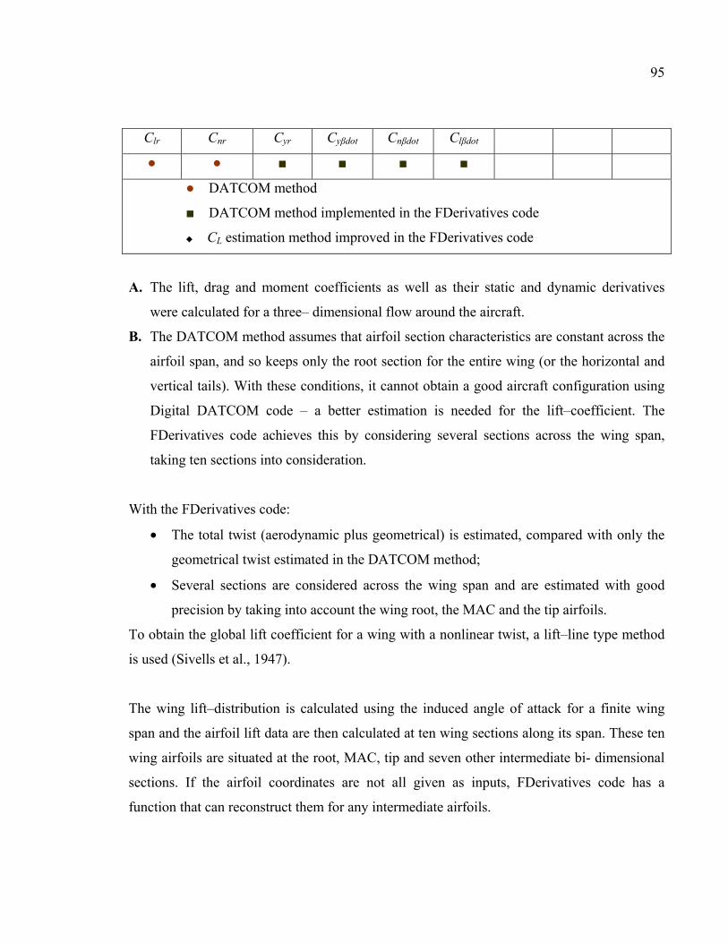
95

Clr Cnr Cyr Cyβdot Cnβdot Clβdot

● ● ■ ■ ■ ■

● DATCOM method

■ DATCOM method implemented in the FDerivatives code

CL estimation method improved in the FDerivatives code

A. The lift, drag and moment coefficients as well as their static and dynamic derivatives

were calculated for a three– dimensional flow around the aircraft.

B. The DATCOM method assumes that airfoil section characteristics are constant across the

airfoil span, and so keeps only the root section for the entire wing (or the horizontal and

vertical tails). With these conditions, it cannot obtain a good aircraft configuration using

Digital DATCOM code – a better estimation is needed for the lift–coefficient. The

FDerivatives code achieves this by considering several sections across the wing span,

taking ten sections into consideration.

With the FDerivatives code:

• The total twist (aerodynamic plus geometrical) is estimated, compared with only the

geometrical twist estimated in the DATCOM method;

• Several sections are considered across the wing span and are estimated with good

precision by taking into account the wing root, the MAC and the tip airfoils.

To obtain the global lift coefficient for a wing with a nonlinear twist, a lift–line type method

is used (Sivells et al., 1947).

The wing lift–distribution is calculated using the induced angle of attack for a finite wing

span and the airfoil lift data are then calculated at ten wing sections along its span. These ten

wing airfoils are situated at the root, MAC, tip and seven other intermediate bi- dimensional

sections. If the airfoil coordinates are not all given as inputs, FDerivatives code has a

function that can reconstruct them for any intermediate airfoils.

96

The determining lift–distribution method used in this code uses successive approximations.

For each airfoil section, a section lift–coefficient distribution is assumed, and then the bi–

dimensional lift coefficients are calculated. Equation (2.1) developed by Phillips et al. (2007)

is used here to estimate the maximum lift coefficient CLmax

( )max max0max0

LL Ls L L L L

L

cC c C

c θ αθ

κ κ κ θΛ=

Λ=

= −

(2.1)

This method applies to any wing geometry, including a twisted wing, and is intended to

replace the old algorithm used in the DATCOM method for a linear twisted wing.

The original formula contained a stall correction factor Lsκ which was eliminated in

FDerivatives code. The maximum lift coefficient for the entire wing is then calculated for

various flight conditions with the following equation:

( )max max0max0

LL L L L L

L

cC c C

c θ αθ

κ κ θΛ=

Λ=

= −

(2.2)

The sweep correction factor depends on the aspect and taper ratios, as shown in eq.(2.3)

1.21 21Lκ κ κΛ Λ Λ≅ + Λ − Λ (2.3)

The maximum lift coefficient of the section maxLc used in eq.(2.2) is calculated in the section

for which the lift coefficient has the highest value. After obtaining the lift distribution along

the wing span, the stall coefficient (corresponding to the maximum lift coefficient) of the

entire wing is obtained using eq.(2.2).

Because the experimental data for W and WB configurations for the Hawker 800XP are

unavailable (are provided by CAE Inc. just for WBT configuration), we need to validate the

results obtained with the FDerivatives code by using other aircraft models founded in the

literature for which experimental data are available for complete aircraft configurations.

The first set of results expressed in terms of lift–coefficient versus the angle of attack is

shown in Figure 2.4 for the wing characteristics (Table 2.2) at Mach number 0.35 and

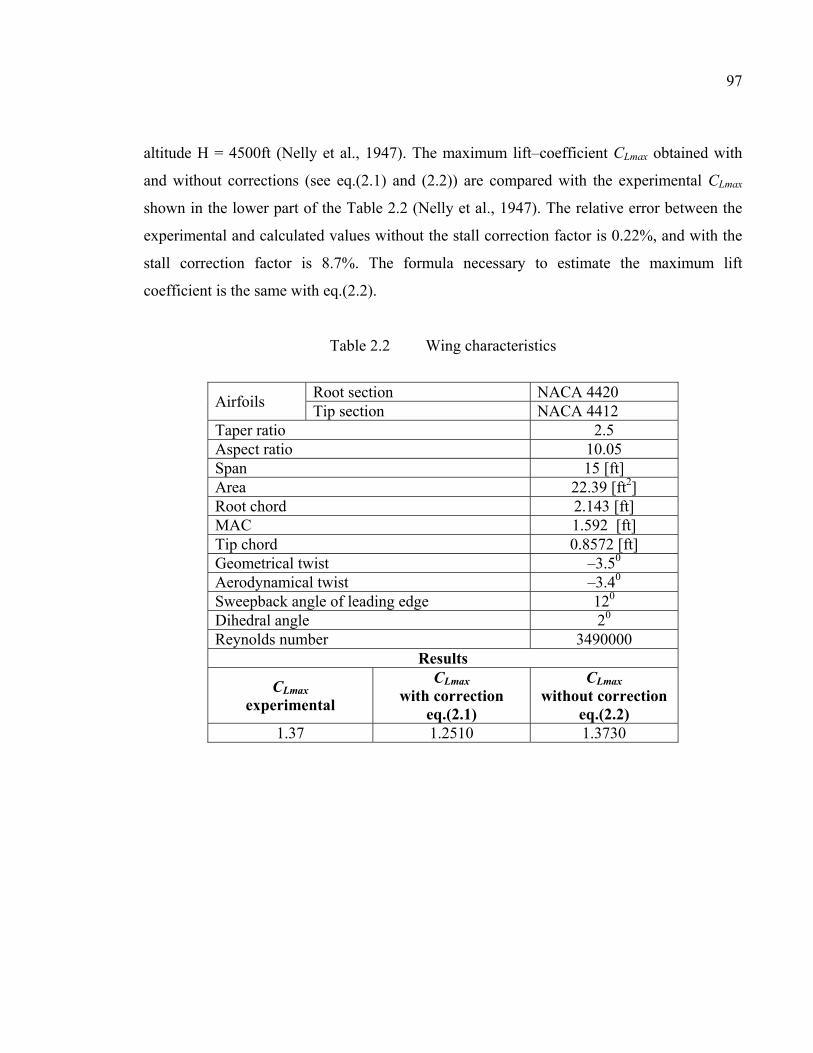
97

altitude H = 4500ft (Nelly et al., 1947). The maximum lift–coefficient CLmax obtained with

and without corrections (see eq.(2.1) and (2.2)) are compared with the experimental CLmax

shown in the lower part of the Table 2.2 (Nelly et al., 1947). The relative error between the

experimental and calculated values without the stall correction factor is 0.22%, and with the

stall correction factor is 8.7%. The formula necessary to estimate the maximum lift

coefficient is the same with eq.(2.2).

Table 2.2 Wing characteristics

Airfoils Root section NACA 4420 Tip section NACA 4412

Taper ratio 2.5 Aspect ratio 10.05 Span 15 [ft] Area 22.39 [ft2] Root chord 2.143 [ft] MAC 1.592 [ft] Tip chord 0.8572 [ft] Geometrical twist –3.50

Aerodynamical twist –3.40

Sweepback angle of leading edge 120 Dihedral angle 20 Reynolds number 3490000

Results

CLmax

experimental

CLmax

with correction eq.(2.1)

CLmax

without correction eq.(2.2)

1.37 1.2510 1.3730

98

Figure 2.5 Lift coefficient distribution for the W configuration at Re = 3.49·106

The lift–coefficient’s curve (Figure 2.5) estimated with the method implemented in

FDerivatives code is contained in the marginal error calculated for the experimental data.

This error represents 3.5% of maximum lift–coefficient provided by the experimental. On the

other hand, the results provided by DATCOM method are quite far from experimental, where

the slope of the lift–coefficient is different and the maximum lift–coefficient appears for a

lower stall angle.

The WB model configuration is presented by Letko et al. (1950), in which the lift and drag

coefficients obtained experimentally for a Mach number of 0.166 and an altitude of 2,075 ft

are also given. The geometrical characteristics for the wing and fuselage are given in Table

2.3.

Table 2.3 Basic model geometrical characteristics

Fuselage Length 40.0 [in] Fineness ratio 6.67

Wing Span 36 [in] Area 324 [in2]

99

Aspect ratio 4.0 Taper ratio 0.6 MAC 9.19 [in] Quarter-chord sweepback angle 00 Twist 00

Dihedral angle 00 Airfoil section NACA 65A008

Figure 2.6 shows the very good validation (near–overlap) of calculated with experimental

lift–coefficient, both versus angle of attack data, using the new FDerivatives code.

Figure 2.6 CL versus α (experimental versus calculated) for WB configuration

C. Better estimation of drag for the WB configuration by using a new nonlinear regression

analysis. Better estimation of pitching moments for the WB configuration.

This method evaluates and combines the isolated moment due to lift of the wing and of the

body, with allowance for their effect on each other. The wing pitching moments due to

effective wing lift includes the effects of body up–wash on the wing and wing carryover onto

the fuselage. These are accounted for on the basis of relations already in the DATCOM

method. Fuselage and nacelles’ free moments due to induced flow from the wing can be

estimated by the technique developed by Multhopp (1942). The sum of these two

100

contributions added to the wing pitching moment due to wing drag gives a better estimation

of the pitching moment than the linear regression analysis method in DATCOM for a WB

configuration.

The new FDerivatives code has changed the way the total moment coefficient is computed.

The nacelles’ contribution is included and the total moment is presented as a sum of the

moment given by the Wing–Body–Nacelles (WBN) and the Horizontal Tail (HT)

contributions:

( ) ( ) ( )0m m mtotal WBN HTC C C= + (2.4)

( )( )

( ) ( )0

0

LC

mm L mWBN WBN WBN

L CG

dCC d C C

dC

α = +

(2.5)

where ( )( )

mm CG

L LCG

CdC x

dC c Cα

α

= +

is estimated as a function of gravitational centre position

and

( ) ( ) ( ) ( ) ( ) ( ) ( )m m m m mfree drag BN W B B WC C C C Cα α α α α +

= + + +

( ) ( ) ( ) ( )( )

00 0 0 0

0 0

m Mm m m mWBN W BN

m M

CC C C C

C=

= + + Δ .

The moment coefficient’s contribution to the body ( )0m BC is defined by Etkin et al. (1996),

where the fuselage’s zero pitching moment coefficients and the two–times–zero pitching

moment coefficients provided by the nacelles are also given. Figure 2.7 shows the moment

coefficients (experimental and calculated) versus the angle of attack.

101

Figure 2.7 Cm versus α (experimental and calculated), WB configuration

D. The longitudinal dynamic stability coefficients CLq and Cmq computed in Digital

DATCOM are assumed to be linear. In the FDerivatives code, these derivatives are

estimated by considering their dependence on the dynamic–pressure ratio ( )q q∞ .These

two derivatives are represented for different Mach numbers versus the angle of attack at

the altitude of 30 ft in Figure 2.8. The linearity appears only if the ratio 1q q∞ = .

102

Figure 2.8 CLq and Cmq versus α, Hawker 800XP, WBT configuration

In addition, CDq is computed in the new code using the method described in DATCOM, and

depends on the pitching rate q, which is defined in the interval [0 to 10] deg/s. The variation

of CDq with the angle of attack for different Mach numbers is presented in Figure 2.9 for M =

0.2 to 0.6 and altitude H = 30 ft in the WBT configuration, where the pitch rate q = 5 deg/s.

Figure 2.9 CDq versus α at the altitude H = 30 ft and q = 5 deg/s

103

E. The zero–lift angle and pitching moment for a wing section are also calculated in the

FDerivatives code, using the thin wing section theory (Abbot, 1959) and a Fourier

method. Very good approximations for the zero–lift coefficients and pitching moments

are obtained using the Pankhurst method (Abbot, 1959).

F. In the subsonic regime, the new FDerivatives code was improved by taking into account

equations for the following dynamic stability derivatives (with the results presented in

Figures 2.10 to 2.12):

• Rolling moment coefficient due to a time variation in the sideslip anglel

C β&for the

WBT configuration,

Figure 2.10 versus α at the altitude H = 30 ft

• Side–force coefficient due to a time variation in the sideslip angley

C β&for the

WBT configuration,

lβC &

104


• The yawing–moment coefficient due to a time variation in the sideslip anglen

C β&

for the WBT configuration.


yβC &

nβC &

105

2.6 Validation results obtained for the entire Hawker 800XP aircraft

Results are presented in terms of stability derivatives for the flight cases expressed by the

following air conditions:

• Altitude = 30.0 ft;

• Mach numbers = 0.2, 0.3, 0.4, 0.5 and 0.6;

• Angle of attack = –5 to 20 deg.

To validate the results, expressed in terms of lift and drag coefficients obtained with the

FDerivatives code, these types of results are compared with the numerical results obtained

from the Digital DATCOM code and experimental Hawker 800XP results (that means the

flight tests), as shown in Figures 2.13 to 2.16, for Mach number M = 0.4, 0.5. The

FDerivatives curves are closer for the experimental data, then the Digital DATCOM code

are. The flight test and geometrical data were provided by CAE Inc for the Hawker 800 XP,

and for this reason, the results are confidential and no numbers are shown on the graphs.

Figure 2.13 CL versus α at M = 0.4

106

Figure 2.14 CD versus α at M = 0.4

Figure 2.15 CL versus α at M = 0.5

107

Figure 2.16 CD versus α at M = 0.5

From the above figures, we can see that differences appear for angles of attack greater than

10 degrees.

Results expressed in terms of derivatives with the exception of the three results presented in

part F (Figures 2.10 to 2.12) obtained with the new FDerivatives code are slightly different

from those obtained with the Digital DATCOM program (Figures 2.17 to 2.24), due to the

fact that FDerivatives code is improved with respect to the DATCOM method implemented

in Digital DATCOM code.

108

Figure 2.17 Cm versus α at Mach number = 0.3

Figure 2.18 Cyβ versus α at Mach number = 0.3

109

Figure 2.19 Clβ versus α at Mach number M = 0.3

Figure 2.20 Cnβ versus α at Mach number M = 0.3

110

Figure 2.21 Cyp versus α at Mach number M = 0.3

Figure 2.22 Cnp versus α at Mach number M = 0.3

111

Figure 2.23 Clp versus α at Mach number M = 0.3

Figure 2.24 Cnr versus α at Mach number M = 0.3

2.7 Conclusions

The new FDerivatives code was conceived by using different methods found in the literature,

along with the main method presented in DATCOM. This new code was designed to obtain

all of the aircraft stability derivatives by considering only a small amount of geometrical data

as inputs. The code is very easy to modify, as it gives the user the possibility to choose the

112

number of derivatives, the aircraft configuration and the flight cases. All the outputs become

inputs for a model that will be implemented in an aircraft simulator at LARCASE laboratory.

The lift–coefficient method implemented in the presented code is better than the lift

calculated with the DATCOM method due to better evaluation of the wing geometry – much

closer to a real wing with changes in geometry and airfoil characteristics, and with a

nonlinear twist. Other derivatives, which are not calculated in the Digital DATCOM code,

are implemented in this new FDerivatives code.

To estimate the aerodynamic characteristics and stability derivatives for a single aircraft

configuration, FDerivatives provides the best results. The user needs only to employ the

proper dimensions for the desired configuration. This code represents a significant amount of

work – it contains over 10,000 lines of MATLAB and 226 text files. Its methodology and a

part of results are validated using the Hawker 800XP aircraft flight tests and the rest of them

are verified with the Digital DATCOM results.

Nicoleta Anton, Ruxandra Mihaela Botez and Dumitru Popescu École de Technologie Supérieure, Montréal, Canada

Laboratory of Research in Active Controls, Aeroservoelasticity and Avionics This article was published in Proceeding of the Institution of Mechanical Engineers, Vol.225,

Part G, Journal of Aerospace Engineering, pp. 403-416, April 2011 DOI: 10.1243/09544100JAERO799

Résumé

Le calcul et la validation des coefficients aérodynamiques et des dérivées de la stabilité de

l'avion X–31 font l'objet de cette étude. Afin d'améliorer les calculs des dérivées de stabilité

d'un avion à aile delta en régime subsonique, un recueil de nouvelles méthodes est

programmé dans un nouveau code, FDerivatives, et ajouté à la méthode classique DATCOM.

Le code FDerivatives est décrit, de même que les améliorations obtenues pour la

configuration de l’avion avec le canard. Toutes les données géométriques requises pour

l'estimation des coefficients aérodynamiques de l'avion X–31 sont calculées pour la

configuration totale de l’avion (aile – fuselage – empennage). Le code Digital DATCOM a

été utilisé pour valider la géométrie et les coefficients aérodynamiques, ainsi que la méthode

implicite et la méthode de Jorgensen. Les résultats expérimentaux sont fournis pour le

modèle X–31 dans la soufflerie à basse vitesse allemande – hollandais (DNW–NWB). Le

code FDerivatives donne de très bons résultats en comparaison avec ces résultats

expérimentaux obtenus en soufflerie. Une analyse du mouvement longitudinal de l’avion X-

31 basée sur des résultats obtenus avec le code FDerivatives, est présentée à la fin de

l’article.

CHAPTER 3

ARTICLE 2: STABILITY DERIVATIVES FOR X-31 DELTA-WING AIRCRAFT VALIDATED USING WIND TUNNEL TEST DATA

114

Abstract

The calculation and validation of the aerodynamic coefficients and stability derivatives for

the X–31 model aircraft are the focus of this study. To improve the stability derivative

calculations for a delta–wing aircraft in the subsonic regime, a compendium of new methods

is programmed into a new code, FDerivatives, and added to the classical DATCOM method.

The FDerivatives code is described, as are the improvements achieved in the aircraft canard

configuration. All of the required geometrical data relative to the aerodynamic coefficient

estimation of the X–31 aircraft are calculated for the Wing–Body–Tail configuration. Digital

DATCOM code was used to validate the geometry and the aerodynamic coefficients, as well

as the implicit method and the Jorgensen method. Experimental results are provided for the

X–31 model in the Low–Speed Wind Tunnel of the German–Dutch Wind Tunnels (DNW–

NWB). The FDerivatives code gives very good results in comparison with experimental

results. An analysis of longitudinal motion, based on FDerivatives results, is presented at the

end.

3.1 Introduction

From a methodological perspective, this paper discusses a qualitative approach and presents

the approaches we used to produce a tool for calculating the aerodynamic coefficients and

derivatives of stability in an open and cooperative fashion. One of the most difficult aspects

of aircraft development is defining the stability and control characteristics. To predict these

characteristics, some tools can be used – wind tunnel tests and flight tests. Flight testing is

more accurate, but it is very expensive. Other methods work with models that have different

levels of fidelity, such as Computational Fluid Dynamics (CFD) for a nonlinear aircraft

model.

Several studies have been conducted on the X–31 aircraft. Yeh et al. (1991) performed

numerical calculations for pre–stall and post–stall flight regimes, including variable canard

115

deflection settings, and the numerical results were compared with wind tunnel and flight test

data.

Phenomena such as wing rock, spins, and departures, which can dominate the high–alpha

behavior of the X–31 configuration and restrict its usable flight envelope, were identified

(Croom et al., 1993) by using dynamic model testing techniques for high angle–of–attack.

The results of these tests have been used to design flight control concepts and configuration

modifications to minimize the adverse effects of these phenomena.

The self–induced roll characteristics of a 2% subscale X–31 aircraft model were investigated

by Williams et al. (1994). Some unusual aerodynamic phenomena have emerged during X–

31 model testing, namely wing rock, HIKR departure, and autorotation.

A method for determining the yawing moment asymmetry from flight data was developed

along with an analysis of the various configuration changes (Cobleigh, 1994). Several

aerodynamic modifications were made to the X–31 forebody with the goal of minimizing the

asymmetry. Applying symmetrical boundary–layer transition strips along the forebody sides

increased the magnitude of the asymmetry and widened the angle-of-attack range over which

the largest asymmetry acted.

For the model at scale 1:5.6 tested in the German–Dutch Wind Tunnels (DNW–NWB), very

few stability derivatives results have been published. Boelens (2009) presents the results

from lift, drag and pitching–moment coefficients and pressure coefficients using the

Computational Fluid Dynamics method employing three leading–edge configurations: all

leading edge flap gaps, only the longitudinal flap gaps, and with no leading edge flap gaps.

In this context, we chose to use the new code, FDerivatives ((Anton et al., 2009), (Popescu,

2009)), developed at the LARCASE laboratory, to estimate the aerodynamic coefficients and

their corresponding stability derivatives. This code was written in MATLAB language and

has a complex structure which contains a graphical interface to facilitate the work of

116

potential users. The static and dynamic derivatives may be estimated based only on

knowledge of the aircraft geometry, using the DATCOM method (Williams et al., 1979a).

The DATCOM procedure is one of the best compilations of knowledge in the field of

analytical calculation of aircraft aerodynamic coefficients and stability derivatives. Designed

as a tool for the evaluation of aerodynamic coefficients and stability derivatives for

preliminary aircraft design, DATCOM provides methods for making these calculations for

various aircraft configurations and different flight regimes, based on the wing geometry. For

the main functions of calculation, the implementation of the general model has been

developed and applied to all the calculation methods used in the code. This facilitates the

replacement of calculation methods, including adding new methods, and simplifies

troubleshooting throughout the code. Also, we have developed a process for the systematic

utilization of various monograms in the DATCOM procedure, incorporating MATLAB’s

interpolation tools.

After these stability derivatives have been calculated, an aircraft’s stability can be determined

for longitudinal and lateral motions. This paper considers only an aircraft’s longitudinal

behavior about the pitch–axis reference frame, presented in the last section. The set of the

first-order linear differential equations was solved for short–period and phugoid motions.

Numerical results are given as eigenvalues, modal damping, natural frequency, magnitude

and phasing, magnitude scaling and phase angle difference. Time–history traces of the short–

period and phugoid responses due to an initial condition of the eigenvector are also

presented. The system’s control response has been investigated using a step control input for

the short–period approximation.

3.2 FDerivatives’ code description

The first main advantage of the FDerivatives code (Anton et al., 2009, Popescu, 2009)

developed at the LARCASE laboratory (www.larcase.etsmtl.ca) with respect to Digital

DATCOM code (Galbraith) is the estimation of the lift, drag and moment coefficients and

their corresponding stability derivatives by use of a minimum of aircraft geometrical data.

117

This data are the area, aspect ratio, taper ratio, sweepback angle and dihedral angle for the

wing, canard and vertical tail. In addition, their coordinates and body parameters are also

determined in the three–dimensional planes.

The FDerivatives program was written based on MATLAB, and has a complex structure

which contains a graphical interface to facilitate the work of potential users.

3.2.1 FDerivatives: Logical scheme and graphical interface

Figure 3.1 shows a brief logical scheme of this code, which works in two steps. The first step

is the pre-processing level, in which the geometry is completely calculated based on initial

characteristics such as the length and the gravity centre position for the fuselage and the

reference area, and on the span, aspect ratio, Mean Aerodynamic Chord (MAC), thickness

ratio, leading–edge sweep (inboard/outboard), semi–span of exposed surface, root chord, tip

chord and MAC for the wing, canard and vertical tail. During the second step, the

aerodynamic coefficients (lift, drag, normal and pitching moment coefficient) for different

flight conditions are calculated. The accuracy of these four aerodynamic coefficients directly

influences the calculation of stability derivatives.

118

Figure 3.1 FDerivatives’ logical scheme

The graphical interface (Figures 3.2 to 3.5) allows users to easily and rapidly change the

aircraft geometrical data for different flight conditions (for the same aircraft configuration, it

will be possible to change only the geometry).

The principle images of the graphical interface are shown for the main window (Figure 3.2),

Wing and Canard parameters (Figure 3.3), Fuselage parameters (Figure 3.4) and Vertical Tail

parameters (Figure 3.5). The results obtained for the Hawker 800XP aircraft, and thus for a

classical Wing–Body–Tail aircraft, were presented by Anton et al. (2009). To obtain the

results presented in this paper for the X–31 aircraft, the code and graphical interface for the

Hawker 800XP were changed, due to the canard configuration, and therefore new functions

were added. FDerivatives code can also be used for a non straight–tapered (double

trapezoidal) wing, and not just for a straight–tapered wing configuration (see Figure 3.3).

119

Figure 3.2 Main window

Figure 3.3 Wing and Canard parameters

120

Figure 3.4 Fuselage parameters

Figure 3.5 Vertical Tail parameters

In the main window, entitled Stability Derivatives (Figure 3.2), the configuration type and

the flight conditions (Mach numbers, altitudes and angles of attack ranges) are defined. It is

possible to fix the wing position and its roughness. For each of the three major surfaces

(Wing, Canard and Vertical Tail), the global parameters and the airfoil coordinates situated at

121

the root, MAC and tip sections are considered. The inputs to the body configuration are the

three parameters: fuselage length, position of the gravitational centre, and fuselage

coordinates (in three dimensions), measured with respect to the reference system.

3.2.2 FDerivatives: functions’ description

FDerivatives code uses a total of 82 MATLAB functions; the aerodynamic coefficients and

their stability derivatives are calculated with 24 of these functions, which are the following:

• 3 functions for lift, drag and moment coefficient estimation (CL, CD and Cm);

• 6 functions for the static derivatives estimation: lift, drag and pitching

moment derivatives due to the angle of attack (CLα, CDα, Cmα); side–force,

yawing, and rolling moments due to the sideslip angle (Cyβ, Cnβ, Clβ); and

• 15 functions for the estimation of the following dynamic derivatives: lift, drag

and pitching moments due to pitch rate derivatives (CLq, CDq, Cmq); lift, drag

and pitching moments due to angle of attack rate derivatives ( ααα DmL CCC ,, );

side–force, rolling and yawing moments due to roll rate derivatives (Cyp, Clp,

Cnp); side–force, rolling and yawing moment due to yaw rate derivatives

(Cyr, Clr, Cnr); and side–force, rolling and yawing moments due to sideslip

angle rate derivatives ( βββ nlY CCC ,, ).

The 58 other functions are needed to calculate the geometrical factors (two- or three-

dimensional) and the aerodynamic functions. The main function of the FDerivatives code is

found in the MATLAB file DATCOM.m, which calls the rest of the MATLAB functions

and text files. The main functions for the aircraft and airfoils’ geometry estimation are

aircraft_geometry.m, to determine the Wing, Canard, Vertical Tail and Body geometries,

and the function airfoil_properties.m which is used to define the geometrical and

aerodynamic characteristics of different airfoils (two- and three- dimensional). The zero–lift

angle and the pitching moment for a wing section are calculated using thin wing section

theory.

122

The inputs to the body configuration are three global parameters: body length, centre of

gravity position at the fuselage station and at the wing level and the fuselage coordinates (in

three–dimensions). The final numerical results are saved in three formats: jpeg, MATLAB

figures and text files.

3.2.3 FDerivatives: Improvements of DATCOM method

All of the improvements have been given in detail ((Anton et al., 2009), (Popescu, 2009)).

Only the improvements that are proposed in the FDerivatives code with respect to the

classical DATCOM method are summarized in this paper. These improvements are:

The lift, drag and moment coefficients as well as their static and dynamic derivatives

calculations for the three- dimensional flow around the aircraft.

The consideration of several sections across the wing span and their estimations with

good precision, found by taking into account the wing root, the MAC and the tip airfoils

(Figure 3.6).

Figure 3.6 Wing geometry for X-31 model aircraft

¬ The obtaining of the lift coefficient CL for a nonlinear twist wing (Figure 3.7).

123

Figure 3.7 Twisted nonlinear wing for the X-31 aircraft

¬ The lift–line type method is used to obtain the global lift coefficient for a

nonlinear twist wing (Sivells et al., 1947).

The wing lift–distribution is calculated using the induced angle of attack for a finite wing

span, while the airfoil lift data are calculated at ten wing sections along its span. These ten

wing airfoils are found at the root, the MAC, the tip and seven other intermediate sections. If

the airfoil coordinates are not all given as inputs, the FDerivatives code has a function that

could reconstruct them for any intermediate airfoils.

A lift-distribution method, using successive approximations, is used in the FDerivatives code.

For each airfoil section, a section lift–coefficient distribution is assumed, for which the two–

dimensional lift coefficients are calculated. Equation (3.1) developed by Phillips et al. (2007)

is used to estimate the maximum lift coefficient CLmax.

( )max max0max0

LL L L L L

L

cC c C

c θ αθ

κ κ θΛ=

Λ=

= −

(3.1)

This method applies to any wing geometry, including to a nonlinear twisted wing, and

replaces the old algorithm used in the DATCOM method for a linear twisted wing.

The sweep correction factor depends on the aspect and taper ratios, as shown in eq.(3.2)

1.21 21Lκ κ κΛ Λ Λ≅ + Λ − Λ (3.2)

The section maximum lift coefficient used in eq.(3.1) is calculated in the section where the

lift coefficient has the highest value. After obtaining the lift distribution along the wing span,

124

the stall coefficient (corresponding to the maximum lift coefficient) is obtained for the entire

wing.

¬ With respect to Digital DATCOM code, the new FDerivatives code, for WB

configuration, gives better estimation of drag using a nonlinear regression

analysis and better estimation of pitching moments.

This method evaluates and combines the isolated moment due to the lift for the WB

configuration, with allowance for their effect on each other. The wing pitching moments due

to the effective wing lift include the effects of body up–wash on the wing and of the wing

carryover onto the fuselage. Fuselage and nacelles’ free moments due to wing-induced flow

can be estimated by the technique developed by Multhopp (1942). The sum of these two

contributions added to the wing pitching moment due to its drag gives a better estimation of

the pitching moment than the linear regression analysis method in the Digital DATCOM

code for a WB configuration.

¬ The zero–lift angle and the pitching moment for a wing section are also

calculated with FDerivatives code using the thin wing section theory (Abbot,

1959) and the Fourier method. Very good approximations for the zero lift

coefficients and pitching moments are obtained using the Pankhurst method

(Abbot, 1959).

3.3 Testing with the X-31 aircraft model

The X–31 aircraft was designed to break the « stall barrier », allowing it to fly at angles of

attack which would typically cause an aircraft to stall resulting in loss of control. The X–31

employs thrust vectoring paddles which are placed in the jet exhaust, allowing the aircraft’s

aerodynamic surfaces to maintain their control at very high angles. For its control, the aircraft

has a small canard, a single vertical tail with a conventional rudder, and wing Leading–Edge

and Trailing–Edge flaps.

125

Figure 3.8 Three-views of the X-31 model

The X–31 aircraft also uses computer controlled canard wings to stabilize the aircraft at high

angles of attack. The stall angle at low Mach numbers is α = 300. The X–31 model geometry

was given by the DLR, at the scale 1:5.6 (Table 3.1) in the AVT–161 meeting. The

geometrical parameters are detailed (Henne et al., 2005).

Table 3.1 Geometrical parameters

Fuselage length 1.725 m

Wing span 1.0 m

Wing Mean Aerodynamic Chord (MAC) 0.51818 m

Wing reference area 0.3984 m2

Wing sweep angle, inboard 57 deg

Wing sweep angle, outboard 45 deg

Canard span 0.36342 m

Canard reference area 0.04155 m2

Canard sweep angle 45 deg

Vertical Tail reference area 0.0666 m2

Vertical Tail sweep angle 58 deg

The main part of the X–31 model (Figure 3.8) is a wing–fuselage section with eight servo-

motors for changing the angles of the canard (δc), the wing Leading–Edge inner/outer flaps

126

(δLei / δLEo), wing Trailing–Edge flaps (δTE) and the rudder (δr) (Rein et al., 2008). The

variation of these angles, for each control surface, is given as:

o Canard: –700 ≤ δc ≤ 200,

o Wing inner Leading-Edge flaps: –700 ≤ δLEi ≤ 00,

o Wing outer Leading-Edge flaps: –400 ≤ δLEo ≤ 00,

o Wing Trailing-Edge flaps: –300 ≤ δTE ≤ 300,

o Rudder: –300 ≤ δr ≤ 300.

The Wing parameters were introduced in Digital DATCOM for the Horizontal Tail and the

Canard as a Wing.

3.4 Validation of the results obtained with the X-31 aircraft

The VN01004 test run was selected from the wind tunnel test data (Henne et al., 2005). This

test took place for angles of attack α = –6° to 55°. The wind tunnel speed was 60 m/s, which

corresponds to Mach number 0.18. The Reynolds number based on the MAC value was Re =

2.07•106, the pressure P = 101045 N/m2 at temperature T = 293.7K, and the altitude was H =

Sea Level. Results are presented in this paper for α = –2° to 20°.

To validate the lift, drag and moment coefficients obtained with both codes, as shown in

Figures 3.9, 3.10 and 3.12, the wind tunnel tests presented in ((Boelens, 2009), (Henne et al.,

2005), (Schütte, 2009)) were chosen. The default method and the Jorgensen method were

both used for this validation. Jorgensen (1978) generated a semi–empirical method to predict

the normal and pitching-moment coefficients, as well as the aerodynamic centre position for

circular and elliptical bodies with and without wings. Method validity is in the range for an

angle of attack of between 0 to 90 degrees.

127

Figure 3.9 Lift coefficient variations with angle of attack

Following the results analysis, shown in Figures 3.9, 3.10 and 3.12, one can say that very

good approximations were obtained with all methods for the range of angle of attack in the

linear zone. Because two codes were used in the paper to generate the results, their

interpretations are made for two zones: the linear zone and the close–to–stall angle zone.

¬ The slopes of the lift coefficient versus the angle of attack are similar, but the

closest curve to the experimental results is obtained with the FDerivatives code.

Table 3.2 Relative errors of lift coefficient variation with angle of attack

Alpha [deg]

Digital DATCOM default method [%]

Digital DATCOM Jorgenson method [%]

FDerivatives code[%]

-2 23.930 31.458 20.735

0 19.134 27.578 18.156

2 16.601 23.205 15.012

4 12.838 19.896 14.012

6 4.647 4.441 7.957

8 4.088 4.262 2.075

10 10.674 11.949 1.885

12 12.931 14.852 1.820

14 15.258 18.005 3.079

16 16.128 19.229 3.722

128

18 16.051 19.120 4.553

20 16.650 19.976 7.197

Relative errors were calculated with the classical formula 100WTT calc

WTT

x xe

x

−= × , where e is the

relative error and xWTT is the value obtained in the wind tunnel. The FDerivatives code results

are the closest to the WTT results, with a relative error smaller than 18% (see Table 3.2).

The fuselage was modeled as a body of revolution using the DLR Wind Tunnel model (see

Figure 3.11).

Figure 3.10 Drag coefficient variations with angle of attack

129

Figure 3.11 X–31 aircraft fuselage, modeled as a revolution body

For angles of attack between 0 and 20 degrees, the best drag coefficient values are obtained

with FDerivatives (see Figure 3.10 and Table 3.3).

Table 3.3 Relative errors of drag coefficient variation with angle of attack.

Alpha

[deg]

Digital DATCOM

default method [%]

Digital DATCOM

Jorgenson method [%]

FDerivatives

code[%]

-2 11.679 9.938 28.286

0 22.071 16.581 12.216

2 32.280 21.749 0.449

4 39.047 24.624 7.670

6 44.470 26.676 11.739

8 50.077 28.596 14.236

10 57.856 30.975 16.498

12 59.603 31.469 15.478

14 53.499 29.681 11.398

16 43.270 26.239 4.901

18 34.429 22.704 2.094

20 26.598 19.012 8.861

130

The pitching moment coefficient is very sensitive to geometrical changes and to the aircraft’s

centre of gravity position. Because all the coefficients presented in this paper were calculated

from the aircraft’s geometry, by considering only a small amount of geometrical data as

inputs, the final results were not the best when extended for moment coefficients. The curve

shapes are similar for the moment coefficient (Figure 3.12), but the maximum and minimum

values obtained by the default method of Digital DATCOM are higher than the wind tunnel

test data. The FDerivatives Cm values are good compared with the wind tunnel tests. The

main structure of the aircraft, without any approximation (the fuselage is not considered as a

revolution body), is modeled using CFD (Boelens, 2009). Differences in results are mainly

seen for angles of attack between 10 to 20 degrees.

Figure 3.12 Pitching moment coefficient variations with angles of attack

Figures 3.13 to 3.15 show the comparison between the stability derivative values obtained

with FDerivatives versus those obtained with Digital DATCOM codes (default & Jorgensen

method).

131

Figure 3.13 Lift and pitch moment coefficients due to the pitch rate (CLq,Cmq ) versus the angle of attack

A very small difference can be seen in Figure 3.14 for lift and pitching moment coefficients

due to the pitch rate calculated with the FDerivatives & Digital DATCOM codes. Very good

results are obtained for yawing and rolling moments and side forces due to roll–rate

derivatives (Figure 3.15).

132

Figure 3.14 Yawing, side force and rolling moments due to the roll-rate derivatives’ variations with the angle of attack

133

Figure 3.15 Side force, yawing and rolling moments due to the sideslip angle derivatives’ variations with the angle of attack

134

135

Figure 3.16 Side force, rolling and yawing moment coefficients variation with angle of attack

Side force, rolling, and yawing moment coefficients are shown in Figure 3.16 with wind

tunnel test data (Schütte, 2009). These derivatives were calculated based on the aircraft’s

geometrical data, which implies the occurrence of small errors, and one can see, in Figure

3.16, the small side force coefficient variation with angle of attack with FDerivatives code, as

well as with the Digital DATCOM code. Very good results were obtained using the

FDerivatives codes for rolling and yawing moment coefficients variation with angle of

attack, and the wind tunnel tests results (see Figure 3.16).

3.5 Longitudinal motion analysis

This paper considers only the aircraft’s longitudinal behavior about the pitch–axis reference

frame. The numerical cases are presented here for three high angles of attack, α = 200, 280,

380, based on the previous results.

We start from the decoupled equations for longitudinal motion with commands fixed. An

aircraft’s mathematical model for longitudinal motion can be represented by a differential

equations system of the form (Schmidt, 1998).

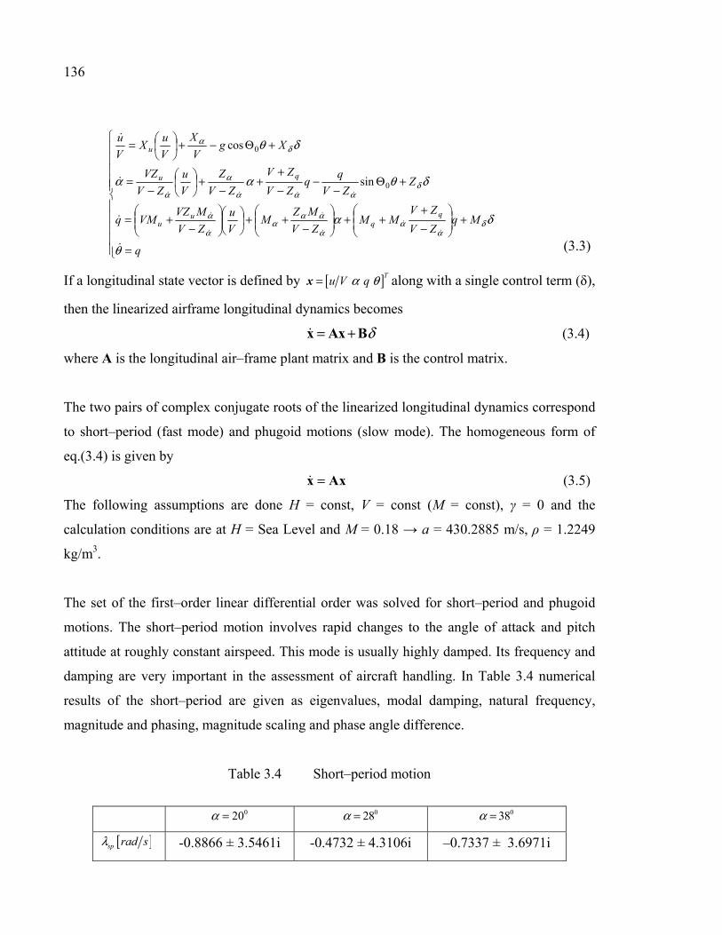
136

=

+

−+

++

−

++

−

+=

+Θ−

−−+

+−

+

−=

+Θ−+

=

q

MqZV

ZVMM

ZV

MZM

V

u

ZV

MVZVMq

ZZV

qq

ZV

ZV

ZV

Z

V

u

ZV

VZ

XgV

X

V

uX

V

u

qq

uu

qu

u

θ

δα

δθαα

δθ

δα

αα

ααα

α

α

δααα

α

α

δα

0

0

sin

cos

(3.3)

If a longitudinal state vector is defined by [ ]Tu V qα θ=x along with a single control term (δ),

then the linearized airframe longitudinal dynamics becomes

δ= +x Ax B (3.4)

where A is the longitudinal air–frame plant matrix and B is the control matrix.

The two pairs of complex conjugate roots of the linearized longitudinal dynamics correspond

to short–period (fast mode) and phugoid motions (slow mode). The homogeneous form of

eq.(3.4) is given by

=x Ax (3.5)

The following assumptions are done H = const, V = const (M = const), γ = 0 and the

calculation conditions are at H = Sea Level and M = 0.18 → a = 430.2885 m/s, ρ = 1.2249

kg/m3.

The set of the first–order linear differential order was solved for short–period and phugoid

motions. The short–period motion involves rapid changes to the angle of attack and pitch

attitude at roughly constant airspeed. This mode is usually highly damped. Its frequency and

damping are very important in the assessment of aircraft handling. In Table 3.4 numerical

results of the short–period are given as eigenvalues, modal damping, natural frequency,

magnitude and phasing, magnitude scaling and phase angle difference.

Table 3.4 Short–period motion

020α = 028α = 038α =

[ ]sp rad sλ -0.8866 ± 3.5461i -0.4732 ± 4.3106i –0.7337 ± 3.6971i

137

[ ]nsp rad sω 3.6553 4.3365 3.7692

spς 0.2425 0.1091 0.1947

u V

q

α

θ

0

0

0

0

0.1386 74.0162

1 0

3.6832 85.2549

1.0076 18.7821

∠ ∠

∠ ∠ −

0

0

0

0

0.1640 89.6792

1 0

4.5056 92.7223

1.0390 3.5417

∠ ∠

∠ ∠ −

0

0

0

0

0.1635 87.1089

1 0

3.8826 87.2358

1.0301 13.989

∠ ∠

∠ ∠ −

q 3.6831 4.5056 3.8827

spφΔ 104.03710 96.26410 101.22500

The pitch attitude appears smaller in magnitude as the angle of attack. A time–history trace

of the short–period response due to an initial condition of the eigenvector is shows in Figure

3.17. The angle of attack and pitch attitude responses are nearly the same for all three angles

of attack. For angles of attack equal to 20 and 38 degrees the response becomes stable at 7

seconds, but for a value of angle of attack close to the stall angle the stabilization time is

more than 10 seconds.

138

Figure 3.17 Short-period response to phasor initial condition

The phugoid mode involves a trade–off between kinetic and potential energy. In this mode,

the aircraft, at nearly constant angle of attack, climbs and slows, then dives, losing altitude

while picking up speed.

Table 3.5 Phugoid motion

020α = 028α = 038α =

[ ]p rad sλ –0.1171 ± 0.3643i –0.2521 ± 0.3491i –0.3936 ± 0.1624i

[ ]np rad sω

0.3826 0.4306 0.4258

pς 0.3060 0.5854 0.9244

139

u V

q

α

θ

0

0

0

0

1 0

0.0434 146.717

0.9069 2.3979

2.3701 110.2176

∠ ∠ −

∠ − ∠ −

0

0

0

0

1 0

0.0296 137.3727

1.1276 0.3939

2.6188 126.2279

∠ ∠ −

∠ − ∠ −

0

0

0

0

1 0

0.0221 145.4172

1.1167 0.4837

2.6225 158.062

∠ ∠ −

∠ − ∠ −

q 0.9068 1.1277 1.1167

[ ]pT s 17.2489 17.9992 38.6864

The angle of attack component is smaller than the u/V component. For this reason, a modal

approximation would typically be based on the assumption that the oscillation occurs with

the aircraft remaining at a constant lift coefficient. The time–history response is shown in

Figure 3.18.

140

Figure 3.18 Phugoid response to phasor initial condition

The stabilization time differs for the three cases. The longest time is for α = 200, up to 50

seconds, after that it diminishes until the 20 seconds for α = 380, and between them the time

of 30 seconds corresponds to α = 280.

The system’s control response has been investigated using a step control input. The

mathematical model which describes the short–period approximation is given by eq.(3.6).

141

( )q

Z Zq

V VZ M Z M

q M M M q MV V

α δ

α α δ αα α δ

α α δ

α δ

= + +

= + + + + +

(3.6)

The control input is a step elevator input with the form given by eq. (2.7)

( ) ( )00

0, 0

, 0e

for tt t

for tδ δ

δ<

= = > (3.7)

The time–history plots of α/δ0 and q/δ0 are shown in Figure 3.19, for time varying from t = 0

to 10 seconds for α = 200 and 380, and from t = 0 to 15 seconds for α = 280. The stabilized

values are shown in Table 3.6.

Table 3.6 Static values for short-period approximation

020α = 028α = 038α =

α/δ0 [rad/rad] -0.2018 2.3857 1.0657 q/δ0 [rad/rad-s] 1.1459 1.3313 1.0308

The positive elevator deflection corresponds to the trailing–edge moving down, which

normally results in negative values for both parameters (α and q) when the aircraft is stable.

Based on the short–period approximation results, the conclusion is that the X–31 aircraft is

not stable for these three angles of attack.

142

Figure 3.19 Short-period response to elevator step input

3.6 Conclusions

The aerodynamic coefficients of the X–31 model aircraft and their stability derivatives were

calculated based on its geometrical data. The codes used to analyze the model were the

classical Digital DATCOM and the FDerivatives code developed at LARCASE laboratory.

Following the AVT–168 meeting, the run test VN01004 (M = 0.18, Re = 2.07•106, P

=101045 N/m2, T = 293.7K) performed in the Low Speed Wind Tunnel of the German–

Dutch Wind Tunnels (DNW–NWB) was used.

143

By taking into account the small number of geometrical parameters, the remaining

geometrical data were calculated to complete the aircraft’s geometry knowledge. The

fuselage was modeled as a body of revolution and the wing was considered as an equivalent

straight tapered platform.

Proper geometry modelling is essential to obtain correct aerodynamic coefficients and their

derivatives. Pitching moment coefficient analysis demonstrates how a correct approximation

of the aircraft’s geometry could be obtained. Lift, drag and pitching moment coefficients, for

angles of attack between –2 and 20 degrees, were calculated with very good accuracy by the

FDerivatives code. In addition, rolling and yawing moment coefficients and side force

coefficients were well–estimated.

For short–period motion the pitch attitude appears smaller in magnitude than the angle of

attack. The angle of attack and pitch attitude responses are nearly the same for all three

angles of attack. For angles of attack of 20 and 38 degrees the response becomes stable at 7

seconds, but for a value of angle of attack close to stall angle the stabilization time is more

than 10 seconds. A modal approximation would typically be based on the assumption that

the oscillation occurs with the aircraft remaining at a constant lift coefficient. Based on the

short–period approximation results, the conclusion is that the X–31 aircraft is not stable for

these three angles of attack.

Nicoleta Anton and Ruxandra Mihaela Botez École de Technologie Supérieure, Montréal, Canada

Laboratory of Research in Active Controls, Aeroservoelasticity and Avionics This article was published in INCAS Bulletin, Vol. 3, Issue 4/2011,

pp. 3-16, ISSN 2066-8201

Résumé

L'analyse de la stabilité d'une configuration de l'avion est étudiée en utilisant une nouvelle

méthode appelé la méthode de la fonctions du poids. Cette nouvelle méthode trouve un

certain nombre de fonctions du poids qui sont égales au nombre d'équations différentielles du

premier ordre. Cette méthode est appliquée sur un avion à aile delta, le X-31, pour les

mouvements longitudinaux et latéraux. Les coefficients aérodynamiques et les dérivés de

stabilité obtenues en utilisant le code numérique Digital DATCOM ont été validés avec les

expériences à basse vitesse en soufflerie données obtenues à l'aide de la soufflerie germano-

néerlandaise (DNW-NWB). La méthode du lieu des racines est utilisée pour valider la

méthode proposée dans cet article.

Abstract

The stability analysis of an aircraft configuration is studied using a new system stability

method called the weight functions method. This new method finds a number of weight

functions that are equal to the number of first-order differential equations. This method is

applied for longitudinal and lateral motions on a delta-wing aircraft, the X-31, designed to

break the « stall barrier ». Aerodynamic coefficients and stability derivatives obtained using

the Digital DATCOM code have been validated with the experimental Low-Speed Wind

CHAPTER 4

ARTICLE 3: THE WEIGHT FUNCTIONS METHOD APPLICATION ON A DELTA-WING X-31 CONFIGURATION

146

tunnel data obtained using the German–Dutch Wind Tunnel (DNW–NWB). Root Locus

Method is used to validate the method proposed in this paper.

4.1 Introduction

Modern fighter aircraft are designed with an unstable configuration or a marginal stability,

and control laws are needed to stabilize the aircraft. A new method for systems stability

analysis, called the Weight Functions Method, is used to analyze the longitudinal and lateral

motions of the X-31.

The X-31 aircraft was designed to achieve its best performance, flexibility and effectiveness

in air combat, due to its canard configuration that provided a better longitudinal

maneuverability. Its aerodynamics contains degrees of non linearity’s that are representative

for a modern fighter aircraft, that was designed to investigate its behavior at high angles of

attack (-5 to 56) degrees.

The mathematical model uses aerodynamic data obtained from wind tunnel tests and the

results provided by Digital DATCOM code, for subsonic speeds. Digital DATCOM code

(Galbraith), known also as DATCOM+, is the first implementation of the DATCOM

procedures in an automatic calculations code. The software is a directly executable portable

application.

Input data, consisting of geometric and aerodynamic parameters of the aircraft, and flight

conditions, are introduced through a text file called « aircraft_name.dcm » whose format is

specific to the software.

The DATCOM+ program calculates the static stability, the high lift and control, and the

dynamic derivative characteristics. This program applies to aircraft flying in the subsonic,

transonic and supersonic regimes, more precisely to traditional wing–body–tail and canard–

equipped aircraft.

147

The computer program offers a trim option that computes control deflections and

aerodynamic data needed to trim the aircraft in the subsonic Mach regimes.

4.2 Weight Functions Method description

In most practical problems, differential equations that model the behaviour of a dynamical

system often depend on more than one parameter. The Lyapunov stability criterion is based

on finding a Lyapunov function. It is not simple and is not always guaranteed to find a

Lyapunov function. The Lyapunov method is very useful, however, when the linearization

around the point of equilibrium leads to a matrix of evolution with eigenvalues having zero

real parts (Stroe, 2008).

The Weight Functions Method (WFM) replaces the classical Lyapunov function finding

problem with a method that finds a number of weight functions equal to the number of the

first order differential equations modeling the system ((Stroe, 2008), (Stroe et al., 2008)).

The difference between the two methods is that the Lyapunov method finds all functions

simultaneously, while the weight functions method finds one function at a time, with their

total number equal to the number of the first order differential equations. For this reason

WFM is found to be more efficient than the Lyapunov method.

For a better understanding of this method, its basic principle is defined in the next system of

eq.(4.1). The coefficients a1i, b1i, c1i, d1i, i = 1÷4 contain the stability derivatives terms. The

x1, x2, x3, x4 represent the unknowns of the system of equations:

1 11 1 12 2 13 3 14 4

2 11 1 12 2 13 3 14 4

3 11 1 12 2 13 3 14 4

4 11 1 12 2 13 3 14 4

f a x a x a x a x

f b x b x b x b x

f c x c x c x c x

f d x d x d x d x

= + + + = + + + = + + + = + + +

(4.1)

148

The total weight function W is defined, in which w1, w2, w3 and w4 are the weight functions

whose sign should be negative to ensure the aircraft stability. In the aircraft model, the sign

of the total function W given by eq.(4.2) should be negative to ensure the aircraft stability.

1 1 11 1 12 2 13 3 14 4 2 2 11 1 12 2 13 3 14 4

3 3 11 1 12 2 13 3 14 4 4 4 11 1 12 2 13 3 14 4

( ) ( )

( ) ( )

W w x a x a x a x a x w x b x b x b x b x

w x c x c x c x c x w x d x d x d x d x

= + + + + + + + ++ + + + + + + +

(4.2)

In our paper, three of the four functions wi : w1, w2 and w3 will be positively defined based on

the sign of the coefficients a1i, b1i, c1i, d1i with i = 1÷4. The last one will be constant and

imposed by the author, w4 > 0. If the positive weight functions will be well defined, then the

sign of total function W will be analyzed in order to identify the stability or instability areas

of the system.

4.3 Application on X-31 aircraft

The X–31 aircraft was designed to break the « stall barrier », allowing the aircraft to remain

under control at very high angles of attack. The X–31 aircraft employs thrust vectoring

paddles which are placed in the jet exhaust, allowing its aerodynamic surfaces to maintain

their control at very high angles.

For its control, the aircraft has a canard, a vertical tail with a conventional rudder, and wing

Leading–Edge and Trailing–Edge flaps.

The main part of the X–31 aircraft model is a wing–fuselage section with eight servo–motors

for changing the canard angles (–700 ≤ δc ≤ 200), the wing Leading-Edge inner/outer flaps (–

700 ≤ δLEi ≤ 00) /(–400 ≤ δLEo ≤ 00 ), the wing Trailing-Edge flaps (–300 ≤ δTE ≤ 300) and the

rudder (–300 ≤ δr ≤ 300) angles (Williams et al., 1994). The X–31 aircraft is capable of flying

at high angles of attack [–50 to 560] and at sideslip angles [–200 to 200].

The aircraft geometrical data are: reference wing area of 0.3984 m2, MAC of 0.51818 m,

reference wing span of 1.0 m. In addition, its mass is 120 kg at Mach number of 0.18 and sea

149

level. The variations of aerodynamic coefficients with angle of attack used in this analysis

have been estimated using the Digital DATCOM code ((Anton et al., 2011), (Anton et al.,

2010)).

4.3.1 Aircraft longitudinal motion analysis

If a longitudinal state vector [ ] [ ]TT xxxxqVu 4321/ == θαx is defined along with a single

control term δ (elevator), then the aircraft’s linearized longitudinal dynamics becomes

(Schmidt, 1999)

long longδ= +x A x B (4.3)

where A is the system matrix and B is the control matrix.

The two pairs of complex conjugate roots of the linearized longitudinal dynamics correspond

to short–period (fast mode) and phugoid (slow mode).

The non dimensional longitudinal equations of motion (4.1) are written, with x1 = u/V, x2 = α,

x3 = q and x4,= θ as follows:

( )( )( )

1 1 2 3 1

2 4 5 6 7 2

3 8 9 10 3

4 11

/

/

/

f a u V a a d

f a u V a a q a d

f a u V a a q d

f a q

α θ δα θ δα δ

= + + +

= + + + +

= + + + =

(4.4)

where the coefficients a1 to a11 are determined with eq.(4.5):

1 2 3 0 4 5 6

7 0 8 9

10 11 1 2 3

, , cos , , , ,

sin , , ,

, 1, , ,

quu

uu

qq

V ZX V Z Zga X a a a a a

V V V Z V Z V Z

V Z M Z Mga a V M a M

V Z V Z V Z

V Z X Z Z Ma M M a d d d M

V Z V V Z V Z

α α

α α α

α α αα

α α α

δ δ δ αα δ

α α α

+= = = − Θ = = =

− − −

= − Θ = + = + − − −

+ = + = = = = + − − −

(4.5)

150

The term (u/V) is then replaced with u . By taking into account eq.(4.4) and (4.5), knowing

the term a7 = 0 (because θ = 0), the final total weight function W becomes:

( ) ( )

( ) ( ) ( )

42 2 2

1 1 2 5 3 10 1 2 2 41

2 6 3 9 3 8 1 3 4 11 1 1 2 2 3 3

k k kk

W w x f w a u w a w a q u w a w a

q w a w a u w a q w a w a q w d u w d w d q

α α

α θ θ δ α=

= = + + + + +

+ + + + + + +

(4.6)

In order to analyze the sign of the total weight function W, it is needed to analyze the signs of

all terms ai, i = 1÷11 and dj, j = 1÷3.

For this reason, the graphs of the variations of coefficients a1 to a11 and d1 to d3 with angle of

attack are shown in Figure 4.1, where it can be seen that the coefficients

1 3 6 110, 0, 0, 0a a a a< < > > as well as other coefficients have fluctuant behavior.

All three terms dj have a oscillating behavior.

Figure 4.1 Coefficients ai and dj variation with the angle of attack

151

The weight functions are chosen considering the signs of the coefficients ai, dj and the tested

cases for the pitch angles θ = [–20 to 20]0 and pitch rates q = [–10 to 10]0/s. The aim of the

WFM is to find 3 positive weighting functions w1, w2 and w3 presented in Figure 4.2, based

on the coefficients variations presented in Figure 4.1.

For the flight case configuration presented in this paper, it is considered that the canard angle

δc = 00 and the flap angle δ = 50. The positive weight functions are defined as:

( )( )( )

2

1 1 2 3 1

222 4 5 6 2

223 8 9 10 3

3 1,100

w u a u a a d

w a u a a q d

w q a u a a q d

w

α θ δ

α α δ

α δ

= + + +

= + + +

= + + +=

(4.7)

and the corresponding final form of the total weight function W is given by eq.(4.8).

( )

( ) ( )

432

1 1 2 2 3 3 4 4 1 2 3 11

3 33 34 5 6 2 6 9 10 3 4 11

k k kk

W w x f w f u w f w f q w f u a u a a d

a u a a d q a u a a q d w q a

α θ α θ δ

α α θ δ α δ θ=

= = + + + = + + +

+ + + + + + + + +

(4.8)

Figure 4.2 Weight functions chosen for longitudinal dynamics

152

a)

b)

c) d)

e) f)

Figure 4.3 Stability analyses with the weight functions method for different values

of constant w4 as a function of angle of attack

Two positives values for w4 are chosen: 1 and 100. It can be observed in Figure 4.3 that the

shape of the stability curve does not change with the values of pitch angle θ and pitch rate q,

153

probably because the terms multiplying the pitch angle are small and constant (a3 = 0.1601

and a11 = 1) as seen also on Figure 4.1; for this reason, their contributions are quite

insignificant in comparison with the rest of the coefficients. Under these circumstances, for

any considered range of pitch rates q and pitch angles θ the system remains always stable.

4.3.2 Aircraft lateral analysis motion

Next, the non-dimensional lateral–directional equations of motion are given in eq.(4.9).

1 2 3 4 1

5 6 7 2

8 9 10 3

11

c c p c c r b

p c c p c r b

r c c p c r b

c p

β β ϕ δβ δβ δ

ϕ

= + + + + = + + +

= + + + =

(4.9)

where

1 2 3 0 4 1

5 6 7

2 8 9

10 3

, , cos , ,

, , ,

, , ,

,

p r

x z x z x zp p r r

x x x

x z x z x zp p

x z z

x z x zr r

z

YY YY Vgc c c c b

V V V V VI I I

c G L N c G L N c G L NI I I

I I Ib G L N c G N L c G N L

I I I

I Ic G N L b G N L

I

β δ

β β

δ δ β β

δ δ

−= = = Θ = =

= + = + = +

= + = + = +

= + = +

11, 1

z

cI

=

(4.10)

The weighting function W can be thus written under the following form, where x1 = β

(sideslip rate), x2 = p (roll rate), x3 = r (yaw rate), x4 = φ (bank angle), x5 = δ:

4

1 1 2 4 3 11

2 6 5 7 2 3 10 8 9 3 4 11

( )

( ) ( )

k k kk

W w x f w c c p c r c b

w p c p c c r b w r c r c c p b w c p

β β ϕ δ

β δ β δ ϕ=

= = + + + + +

+ + + + + + + +

(4.11)

All possible positive and negative values of sideslip rate, roll rate, yaw rate and bank angle

were considered. To analyze the sign of the weight function W, the sign of terms ci, i =

1÷11and bj, j = 1÷3 where analyzed. In Figure 4.4, it can be observed that b1, b2, b3 < 0, c1,

154

c2, c4, c5, c9 < 0 and c3, c11 > 0, while a non linear behavior can be seen for the other four

coefficients c6, c7, c8 and c10 presented.

In eq.(4.11), the parenthesis which multiplies the first term is negative

)( 13421 bcrcpcc δφβ ++++ . For positive values of β, this term is always negative. We

know that c1 < 0, and for this reason the first weighting function w1 = c12/β2. Equation (4.11)

becomes:

21

1 2 4 3 1 2 6 5 7 22

3 10 8 9 3 4 11

( ) ( )

( )

cW c c p c r c b w p c p c c r b

w r c r c c p b w c p

β β ϕ δ β δβ

β δ ϕ

= + + + + + + + + +

+ + + + (4.12)

Figure 4.4 The ci and bj coefficients’ variation with the angle of attack

The parenthesis which multiplies w2p is also negative 0)( 2756 <+++ brccpc δβ . Based on

its sign the second function w2 are defined as 22756

22 )( brccpcpw δβ +++= .

155

The total function W is now given by eq.(4.13).

22 21

1 2 4 3 1 6 5 7 22

6 5 7 2 3 10 8 9 3 4 11

( ) ( )

( ) ( )

cW c c p c r c b p c p c c r b

p c p c c r b w r c r c c p b w c p

β β ϕ δ β δβ

β δ β δ ϕ

= + + + + + + + + ×

+ + + + + + + + (4.13)

At this point it is possible to define w3 or w4 as a positive constant. Because c11 > 0, it was

chosen φpcw 114 = . The final form of function W is given by eq.(4.14).

23 31

1 2 4 3 1 6 5 7 2

23 10 8 9 3 11

23 2 2 2 3 311 2 4 3 1 11 6 5 7 2

3 10 8 9 3

( ) ( )

( ) ( )

( ) ( )

( )

cW c c p c r c b p c p c c r b

w r c r c c p b c p

cc c p c r c b c p p c p c c r b

w r c r c c p b

β ϕ δ β δβ

β δ ϕ

ϕ δ ϕ β δβ

β δ

= + + + + + + + + +

+ + + + + =

= + + + + + + + + + +

+ + + +

(4.14)

Two of the weighting functions chosen have a constant variation with angle of attack (w1 and

w4); w2 is variable and the last one is defined as w3 = 1 and 100.

It was considered that the roll rate p = [–6 to 6]0/s, the yaw rate r = [–2 to 2]0/s, the sideslip

rate β = [–10 to 10]0 and the bank angle Φ = [–30 to 30]0.

Figure 4.5 Weight functions chosen for the lateral dynamics

156

a)

b)

c)

d)

Figure 4.6 Lateral-Directional stability analysis with the weight functions method for different values of constant w3 as a function of angle of attack

For the lateral motion, the weight functions are overlapped only if p, r, β and φ are zero; that

means the value chosen for the weight function w3 have no influence on the total weight

function W. The system is stable for roll, spiral and Dutch roll modes as the total weight

function W is negative as shown in Figure 4.6 for extreme values chosen for p, r, β and φ .

For the studied case, the X-31 aircraft is stable for any type of motion within limits for p, r,

β , φ (short-period, phugoid, roll, Dutch roll and spiral modes).

4.4 Root Locus Map

The five modes of motion for the X-31 aircraft are: the short period and the long period for

longitudinal motion of the aircraft and the roll, Dutch roll and spiral for lateral motion. The

157

natural frequency (ωn) and the damping ratio (ζ) are defined for each mode from the values

of the eigenvalues. For the longitudinal stability analysis, two modes are studied: the short

period and the phugoid. The short term pitch is a second order response. The phugoid mode

is the long–term motion of an aircraft after a disturbance.

The matrices of eq.(4.3) are given in the next eq.(4.15), as described by Schmidt (1999):

0

0,

0

0 0 1 0

, ,

0

u

qu

long

quu q

long long long e

X gX

V VV ZV Z Z

V Z V Z V Z

V ZV Z M Z MV M M M M

V Z V Z V Z

X

Vu

Z

V Z uq

Z MM

V Z

α

α

α α α

α α αα α

α α α

δ

δ

α

δ αδ

α

αδ

θ

−

+ − − −=

+ + + + − − −

Δ Δ −= = = Δ Δ +Δ −

A

x B

(4.15)

The roots of the characteristic equation det (λ I – Along) = 0 gave these eigenvalues λ1 to λ4.

For both longitudinal modes, the natural frequency ωn and damping ratio ζ are estimated

directly from the characteristic equation 0=− longAIλ , as function of the longitudinal

eigenvalues (eq.(4.16)); the eigenvalues λ1,2 correspond to short-period and λ3,4 to phugoid

modes.

( )

( )( )

( )1,2 3,4

2 21,2 3,4

Re Re,

1 Im 1 Im

n n

n n

ςω λ ςω λ

ω ς λ ω ς λ

= =

− = − =

(4.16)

158

A representation of the eigenvalues obtained for the longitudinal motion of an X-31 aircraft

is shown in Figure 4.7. All real parts of eigenvalues are negative, which means that the X-31

aircraft is stable in its longitudinal motion.

Figure 4.7 Root locus map longitudinal motion of the X-31 aircraft

The matrices of the aircraft lateral model are next defined in eq.(4.17), based on (Schmidt,

1998).

00

cos

0,

0

0 1 0 0

,

p r

x z x z x zp p r r

x x xlat

x z x z x zp p r r

z z z

x z

lat lat

YY Y V g

V V V u

I I IG L N G L N G L N

I I I

I I IG N L G N L G N L

I I I

Y

VI

G L Np

r

β

β β

β β

δ

δ δ

θ

β

φ

− + + + =

+ + +

Δ +Δ = = Δ Δ

A

x B ,

0

x lat a

x z

z

I u

IG N L

Iδ δ

δ

= Δ + (4.17)

159

Three modes are considered in the aircraft lateral motion modeling:

• Spiral mode representing, a convergent or a divergent motion;

• Roll mode representing a fast convergent motion, and

• Dutch roll mode representing a light damped oscillatory motion with a low frequency.

These modes are significant factors mainly in the uniform cruise flight. For the lateral aircraft

motion modelling, two real roots correspond to roll and spiral modes, and a pair of complex

roots correspond to Dutch roll mode obtained from the characteristic equation 0=− latAIλ .

The rolling motion is generally very much damped and reaches the steady state in a very

short time. An unstable spiral mode results into a turning flight path. The Dutch roll is a

nuisance mode that appears in the basic roll response to lateral control and can induce non–

controlled and non–desired motions in roll and yaw modes. These motions can significantly

influence the ability of the pilot to control the lateral–directional motions with precision.

The eigenvalues for all three motions described above for X-31 aircraft are represented in

Figure 4.8: blue for Dutch Roll, red for spiral and green for roll mode.

Figure 4.8 Root locus map for lateral motion

160

Results obtained with the weight functions method shown in Figure 4.6, have proven that the

aircraft is stable in its lateral motion. Results presented with root locus map presented in

Figure 4.8 show that the X-31 aircraft has a stable lateral motion, because all eigenvalues

calculated with the root locus map are situated in the negative plane. The Handling Qualities

Method could be used in further studies to determine the aircraft stability (Hodgkinson,

1999), (Bihrle, 1965), (Cotting, 2010).

4.5 Conclusions

A stability analysis based on the null solutions stability studies for differential equation

systems was presented in this paper. The main aim was to found the positive weight

functions in order to analyze the X-31 aircraft stability. The aerodynamics coefficients and

their stability derivatives were determined with Digital DATCOM code. Based on the

aircraft’s aerodynamic model in the WFM, 3 functions were defined as function of stability

derivatives terms, and the last fourth function was considered positive and chosen to be 1 and

100. The WFM was applied for longitudinal and lateral motions. A discussion of results was

done for each case, and the stability was defined and is summarized in the previous sections.

HQM was also applied to validate the aircraft stability results found with WFM.

X-31 has a stable longitudinal and lateral dynamics. For the considered altitude and Mach

number, the aircraft was found to be stable, regardless the angle of attack. Both modes tested

here, the slow and the fast, did not induced any oscillations and/or instabilities.

CHAPTER 5

ARTICLE 4: WEIGHT FUNCTIONS METHOD FOR STABILITY ANALYSIS APPLICATIONS AND EXPERIMENTAL VALIDATION FOR HAWKER 800XP

AIRCARFT


Laboratory of Research in Active Controls, Aeroservoelasticity and Avionics This article was presented at AIAA Modeling and Simulation Technologies Conferance 13-

16 August 2012, Minneapolis, Minnesota, DOI: 10.2514/6.2012-4718

Résumé

Les coefficients de portance, traînée et du moment ainsi que leurs dérivées de stabilité ont été

obtenues en utilisant le code récent FDerivatives développé à LARCASE et le code Digital

DATCOM écrit en Fortran. Les résultats obtenus par l'utilisation de ces codes ont été validées

avec les données d'essais en vol fourni par CAE Inc., pour le Hawker 800XP, un avion

d'affaires de taille moyenne, bimoteur avec les ailes d'une seule pièce. Ensuite, à l'aide de

deux méthodes, ces résultats ont été utilisées pour analyser la stabilité de l’aéronef: 1) La

méthode des fonctions du poids (WFM) et 2) La méthode des qualités de vol (HQM). La

méthode WFM trouve un nombre de fonctions de poids qui sont égales au nombre

d'équations différentielles nécessaires à la modélisation du système. La méthode HQM

détermine la stabilité de l’avion à partir du signe de la partie réelle des valeurs propres. Le

WFM détermine la stabilité de l'avion en fonction du signe de la fonction total du poids. Les

signes devraient être négatifs dans les deux méthodes. Les cas de vol suivants sont

considérés: le nombre de Mach = 0.4 et 0.5, altitude = 5000 m, 8000 m et 10000 m, et les

angles d'attaque α = -50 à 200. Par conséquent, la stabilité des avions est validée en utilisant

deux méthodes: le WFM et HQM. L'originalité du travail se trouve dans la validation de la

WFM à une analyse de stabilité appliquée à un avion réel.

162

Abstract

A new method for system stability analysis, the weight functions method, is applied to

estimate the longitudinal and lateral stability of a Hawker 800XP aircraft. This paper assesses

the application of the weight functions method to a real aircraft and a method validation with

an eigenvalues stability analysis of linear small-perturbation equations. The method consists

of finding the weight functions that are equal to the number of differential equations required

for system modelling. The aircraft’s stability is determined from the sign of the total weight

function - the sign should be negative for a stable model. Aerodynamic coefficients and

stability derivatives of the mid-size twin-engine corporate aircraft Hawker 800XP are

obtained using the in-house FDerivatives code, recently developed at our laboratory of

applied research in active controls, avionics and aeroservoelasticity LARCASE, with the

results validated with the flight test data supplied by CAE Inc. This aircraft model was

selected because it was part of a research project for FDerivatives code; continued with the

weight functions method for stability analysis in order to develop a design tool, based only

on aircraft geometrical parameters for the subsonic regime. The following flight cases are

considered: Mach numbers = 0.4 and 0.5, altitudes = 3000 m, 5000 m, 8000 m and 10000 m,

and angles of attack α = -50 to 200.

5.1 Introduction

Modern fighter aircraft are designed with an unstable configuration which gives marginal

stability. A control law is necessary to stabilize the aircraft. Aerodynamic models contain

nonlinearities representative of a modern fighter. The stability analysis for a real aircraft was

done in this paper using the longitudinal and the lateral-directional motion mathematical

model. The mid-size Hawker 800XP is a twin-engine corporate aircraft with low swept-back

one-piece wings, a high tailplane and rear-mounted engines, for which the maximum Mach

number is 0.9. This aircraft operates in the subsonic and transonic regimes; the flight test data

were provided by CAE Inc. A new method for systems stability analysis, the weight

functions method, was used to replace the use of Lyapunov functions. This method can be

163

used as a design tool because it can be applied if an aircraft's geometrical parameters are

known.

The Weight Functions Method (WFM) has been used mostly for crack problems, to

determine stress factors. The method was applied by Yoichi et al. (2003) to solve two- and

three-dimensional crack problems, to calculate stress intensity factors for arbitrary loading

conditions. The stress intensity factor for a patched crack within an infinite plate was

successfully numerically validated using the WFM (Kim et al., 2000). Different formula to

calculate the stress intensity factor are presented by (Paris et al., 1976), (Wu et al., 1983),

(Fett, 1991), (Schneider et al., 1989).

A different approach was presented by Stroe (2008), who solved the Lurie-Postnikov

problem using general equations for linear or nonlinear vibrations by linear transformations.

Stroe also analyzed a holonomic system with dependent variable equations where the weight

functions method was applied for vibration and stability studies in the cases of linear and

nonlinear damped holonomic systems (Stroe et al., 2008).

The WFM has been applied in the aerospace industry for the modelling of the longitudinal

motion of a canard configuration generic fighter aircraft, called the High Incidence Research

Model (HIRM) by the first author of this paper, Anton (2005). The HIRM, a non-linear

aircraft model developed by FOI, the Swedish Defense Research Agency based on the

Generic Aerodata Model (GAM) developed by SAAB AB, has been the subject of

collaboration within the Group for Aeronautical Research and Technology in EURope

(GARTEUR Action Group FM (AG08)). The results were presented for a complete range of

angle of attack [-10 to 30]0 and elevon deflection angle [-30 to 30]0, constant value of Mach

number of 0.25 and altitude 500 m. The WFM was applied in the case of short-period

longitudinal approximations for the system of equations with unstable characteristics given

by the pitching-moment coefficients, and the aircraft model was stabilized using control

laws. The stability field was augmented from an angle of attack of 10.9 degrees up to 26

164

degrees. This model had increased complexity because the thrust component was included in

the system equations.

In this paper, the WFM and the eigenvalues stability method are applied to study the Hawker

800XP aircraft’s stability, based on aerodynamic coefficients and their derivatives provided

by the FDerivatives code (Anton et al., 2010). This is the first time that the weight functions

method is being used to analyze longitudinal and lateral aircraft model stability. The WFM is

used here to model the stability of a mid-size business aircraft with a typical wing-body-tail

configuration and three basic control surfaces: the ailerons, elevator and rudder, designed to

change and control the moments about the reference axis. This airplane has swept-back

wings that are used to delay the drag divergence.

The results, expressed in terms of weighting functions for the WFM, and in terms of damping

and frequency for the eigenvalues method, are presented for the subsonic regime

characterized by Mach numbers equal to 0.4 and 0.5, and four altitudes: 3,000 m, 5000 m,

8000 m and 10000 m. The pitch angles θ = [-20 to 20]0 and pitch rates q = [-3.5 to 3.5] 0/s are

the longitudinal motion variables, and the roll rate p = [-6 to 6]0/s, yaw rate r = [-2 to 2]0/s,

sideslip angle β = [-5 to 5] 0 and roll angle Φ = [-15 to 15] 0 are the variables for lateral

motion. It was also considered that we have a value δ = 50 for the control term. In the

following sections, the WFM and root locus method are described and the related results

using both methods are presented.

5.2 The Weight Functions Method

Quadratic forms have a matrix representation, and studying their representation can be

reduced to a study of symmetric matrices. Consider the function F: R2→R, where F = a11x12

+ a12x1x2 + a22x22 (Wilde, 2011). This quadratic form in Rn is ( )

, 1

n

ij i ji j

F x a x x=

= , where x = (x1, ...,

xn), and the matrix A is a unique and n x n symmetric matrix. The matrix A is:

1) positive definite if F(x) > 0, for x ≠ 0 in Rn. x = 0 is a unique global minimum of the

quadratic form given by A.

165

2) positive semidefinite if F(x) ≥ 0, for x ≠ 0 in Rn. x = 0 is a global minimum, but not a

unique global one, of the quadratic form given by A.

3) negative definite if F(x) < 0, for x ≠ 0 in Rn. x = 0 is a unique global maximum of the

quadratic form given by A.

4) negative semidefinite if F(x) ≤ 0, for x ≠ 0 in Rn. x = 0 is a global maximum, but not a

unique global one, of the quadratic form given by A.

5) indefinite if F(x) > 0, for some x ∈Rn and < 0 for some other x ∈Rn. x = 0 is neither a

maximum nor a minimum of the quadratic form given by A.

In most practical problems, differential equations that model the behavior of a dynamic

system often depend on more than one parameter. For example, the WFM is more efficient

than the classical Lyapunov functions method since only one function has to be found at a

time, while the Lyapunov method finds all the functions simultaneously. In fact, the

Lyapunov stability criteria are based on finding only one Lyapunov function. Finding a

Lyapunov function is not simple and is not guaranteed.

The WFM finds a number of weight functions that is equal to the number of the first-order

differential equations modelling the system (Stroe, 2008), (Stroe et al., 2008).

Theorem (Stroe et al., 2008): Given the autonomous system ( ) , nx f x x R= ∈ , if wk (x1, x2... xn)

exist such that 1

n

k k kk

dV x w dx=

= is a total exact differential, then the stability is given by

1

n

k k kk

W x w f−

= as follows: W is negative-definite, the solution is asymptotic stable; W is the null

function, the solution is simple stable; W is positive-definite, the solution is unstable.

wk represents the weight functions, with k = number of equations and unknowns, and fk are

the functions equivalent to the derivatives of xk variables.

Four positive-defined weight functions are considered in this paper; three expressed as

functions of the system’s coefficients and determined gradually, and the last being positive-

166

constant defined. The fourth weight function, defined as 1 (the smaller positive integer) or

100 (a high positive integer) are utilized to analyze the longitudinal and lateral-directional

stability of the Hawker 800XP aircraft. Both values of the last weight function have been

considered in order to determine if the stability does (or does not) depend on its order of

measure. The analysis of the WFM results was conducted based on the values of the

aerodynamic coefficients and stability derivatives estimated from the aircraft geometry, and

were validated with flight test data.

5.3 Description of the model

5.3.1 Longitudinal motion

Longitudinal dynamic stability is characterized by short-period and phugoid modes (Schmidt,

1998). If a longitudinal state vector [ ]Tu V qα θ=x is defined along with a single control

term δ, then the aircraft’s equations of motion for the linearized longitudinal motion become:

x = Ax + Bδ (5.1)

where A is the plant matrix and B is the control matrix. The two pairs of complex conjugate

roots of the linearized longitudinal dynamics correspond to the short-period (fast) and

phugoid (slow) modes. The homogeneous form of eq.(5.1) is given by

x = Ax& (5.2)

Equation (5.1) can be further represented as eq.(5.3), using following notations:

( )( )( )

1 1 2 3 1

2 4 5 6 7 2

3 8 9 10 3

4 11

f a u V a a d

f a u V a a q a d

f a u V a a q d

f a q

α θ δα θ δα δ

= + + +

= + + + +

= + + + =

(5.3)

where the functions f1, f2, f3 and f4 are equivalent to derivatives of x1, x2, x3 and x4. The right

hand coefficients of eq.(5.3) are the following:

167

1 2 3 0

4 5

16 7 0

2

38 9

4

10 11

1

, , cos ,

, ,

, sin

,, ,

, 1

u

u

qlong

long

ulongu

long

qq

X ga X a a

V VVZ Z

a aV Z V Z

V Z gx u Va a

V Z V Zx

VZ M Z Mx q a VM a MV Z V Zx

V Za M M a

V Z

Xd

α

α

α α

α α

α α αα

α α

αα

α

θ

= = = − Θ

= =− −+= = = − Θ − −=

= = + = + − − =+

= + = −

=

& &

& &

& &

& &

&&

2 3, ,Z Z M

d d MV V Z V Z

δ δ δ αδ

α α

= = + − −&

& &

(5.4)

In the next equation, the term (u/V) is then replaced withu . By taking the above two

equations into account and knowing that the term a7 = 0, and that the unknowns x1long, x2long,

x3long and x4long have been defined in eq.(5.4), the total weight function Wlong is defined by:

( ) ( )

( )

4

1 1 2 3 1 2 5 4 6 21

3 10 9 8 3 4 11

long k k k long longk

long long

W w x f w u a u a a d w a a u a q d

w q a q a a u d w a q

α θ δ α α δ

α δ θ=

= = + + + + + + + +

+ + + + +

% % %

% (5.5)

5.3.2 Lateral motion

Lateral-directional motion equations are given in matrix form as eq.(5.1). Therefore, the

initial system can be written as follows:

1 1 2 3 4 1

2 5 6 7 2

3 8 9 10 3

4 11

f c c p c c r b

f c c p c r b

f c c p c r b

f c p

β φ δβ δβ δ

= + + + + + + + = + + + =

= (5.6)

where f1, f2, f3 and f4 are given by the left hand side of eq.(5.7) and the coefficients of eq.(5.6)

are expressed as functions of the stability derivative values on the right hand side of eq.(5.7):

168

1 2 3 0 4 1

5 6

17 2

2

38 9

4

, , cos , ,

, ,

,

,

,

p r

xz xzp p

x x

xz xzlatr r

x xlat

lat xz xzp p

z zlat

YY YY Vgc c c c b

V V V V V

I Ic L N c G L N

I I

I Ix c G L N b G L NI Ix p

x r I Ic N L c G N L

I Ix

G

G

β δ

β β

δ δ

β β

β

φ

−= = = Θ = =

+ = +

= = + = + =

= = + = + =

=

10 3

11 1 2 3

,

,

1, , ,

xz xzr r

z z

xz xz

x z

I Ic G N L b G N L

I I

Y I Ic b b G L N b G N L

V I I

δ δ

δδ δ δ δ

= + = +

= = = + = +

(5.7)

The function Wlat can be written for aircraft lateral motion in the following general form,

where x1lat = β, x2lat = p, x3lat = r and x4lat = φ:

( )

( ) ( )

4

1 1 2 4 3 11

2 6 5 7 2 3 10 8 9 3 4 11

lat k k k latk

lat lat lat

W w x f w c c p c r c b

w p c p c c r b w r c r c c p b w c p

β β φ δ

β δ β δ φ=

= = + + + + +

+ + + + + + + + +

(5.8)

5.4 Results obtained using the weight functions method for the Hawker 800XP aircraft

The Hawker 800 XP aircraft has the following main geometrical characteristics: reference

wing area of 34.75 m2, reference wing span of 15.66 m, mean aerodynamic chord of 2.44 m

and a mass of 12,701 kg. The flight cases are characterized by two Mach numbers: 0.4 and

0.5, four altitudes of 3,000 m, 5,000 m, 8,000 m and 10,000 m, and various angles of attack

between -40 and 200.

Stability derivatives for the Hawker 800XP aircraft were determined using the new

FDerivatives code (Anton et al., 2010), (Anton et al., 2011) dedicated to the analytical and

numerical calculation of aerodynamic coefficients and their corresponding stability

derivatives.

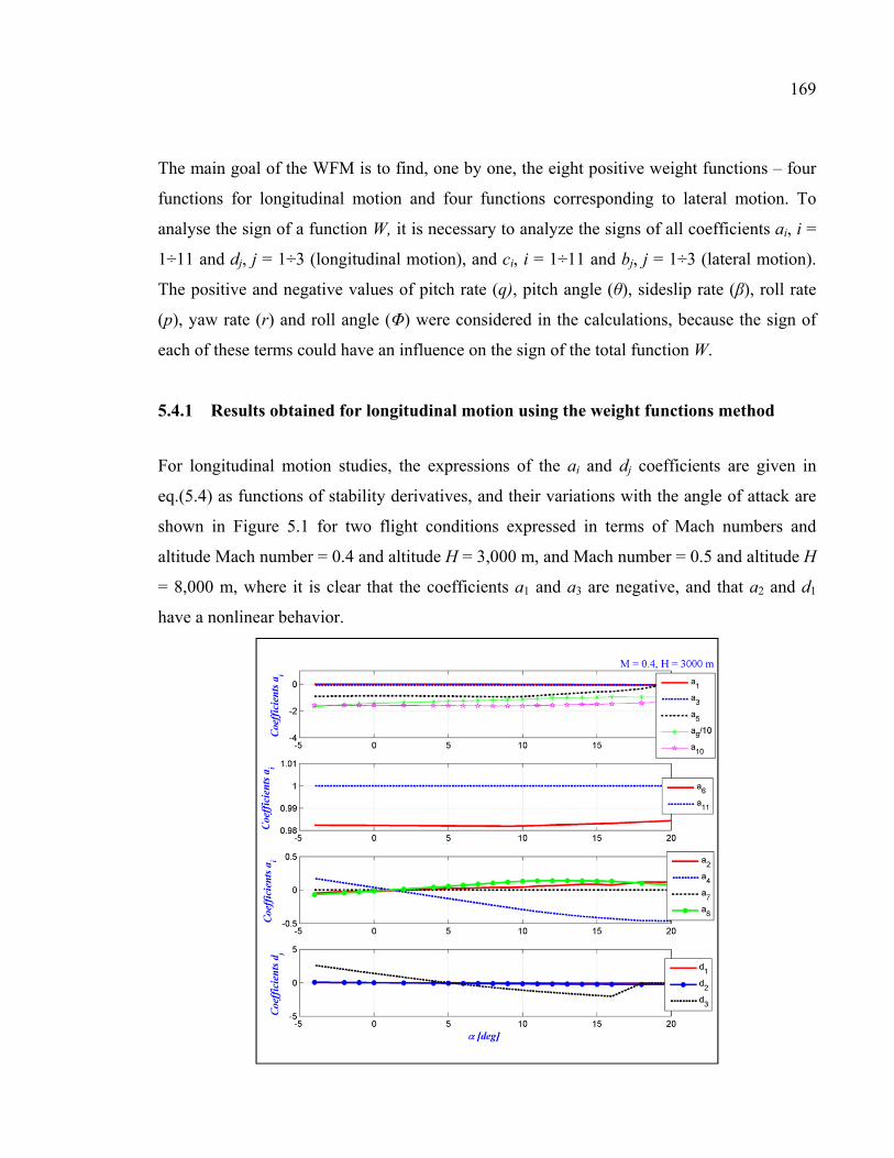
169

The main goal of the WFM is to find, one by one, the eight positive weight functions – four

functions for longitudinal motion and four functions corresponding to lateral motion. To

analyse the sign of a function W, it is necessary to analyze the signs of all coefficients ai, i =

1÷11 and dj, j = 1÷3 (longitudinal motion), and ci, i = 1÷11 and bj, j = 1÷3 (lateral motion).

The positive and negative values of pitch rate (q), pitch angle (θ), sideslip rate (β), roll rate

(p), yaw rate (r) and roll angle (Φ) were considered in the calculations, because the sign of

each of these terms could have an influence on the sign of the total function W.

5.4.1 Results obtained for longitudinal motion using the weight functions method

For longitudinal motion studies, the expressions of the ai and dj coefficients are given in

eq.(5.4) as functions of stability derivatives, and their variations with the angle of attack are

shown in Figure 5.1 for two flight conditions expressed in terms of Mach numbers and

altitude Mach number = 0.4 and altitude H = 3,000 m, and Mach number = 0.5 and altitude H

= 8,000 m, where it is clear that the coefficients a1 and a3 are negative, and that a2 and d1

have a nonlinear behavior.

170

Figure 5.1 The ai and dj coefficients’ variation with the angle of attack for Mach numbers M = 0.4 at altitude H = 3,000 m and M = 0.5 at

H = 8,000 m

The first term of eq.(5.5), ( )1 1 2 3 1longw u a u a a dα θ δ+ + +% % ,, is negative, since

( )221 2 3 1longw u a a dα θ δ= + +% is positive, and the quantity within the parenthesis multiplying

w1long should be negative to respect the stability requirements.

( ) ( )

( )

331 2 3 1 2 5 4 6 2

3 10 9 8 3 4 11

long long

long long

W u a u a a d w a a u a q d


α θ δ α α δ

α δ θ

= + + + + + + + +

+ + + + +

% % %

% (5.9)

In the second term of eq.(5.9), which should be negative to respect the stability requirements,

the coefficient multiplying w2long should also be negative, since 2 22 5 0longw aα= > .

( ) ( )

( )

33 2 21 2 3 1 5 5 4 6 2

3 10 9 8 3 4 11

long

long long

W u a u a a d a a a u a q d


α θ δ α α δ

α δ θ

= + + + + + + + +

+ + + + +

% % %

% (5.10)

171

In the third term of eq.(5.10), the third weighting function is

( )223 8 9 3 0longw q a u a dα δ= + + >% . The last positive function is defined as w4long = 1 or 100.

( ) ( )( ) ( )

33 2 21 2 3 1 5 5 4 6 2

238 9 3 10 9 8 3 4 11

long

long

W u a u a a d a a a u a q d

q a u a d a q a a u d w a q

α θ δ α α δ

α δ α δ θ

= + + + + + + + +

+ + + + + + +

% % %

% % (5.11)

In the new wi functions defined above (eq.(5.9) to (5.11)) we have obtained the final form of

the Wlong function for the aircraft longitudinal motion, expressed in the following equation:

( )( )( )

( ) ( )

231 2 3 1 2 3 1

3 4 2 3 2 3 2 35 4 5 5 6 5 2

2310 9 8 3 8 9 3 4 11

long

long

W u a u a a d a a d

a a a u a a q a d

q a q a a u d a u a d w a q

α θ δ α θ δ

α α α δα

α δ α δ θ

= + + + + + +

+ + + + +

+ + + + + + +

% %

%

% %

(5.12)

For two cases: Mach numbers 0.4 and 0.5 with corresponding altitudes of 3,000 m and 8,000

m, respectively, the variations of the positive weight functions w1long, w2long and w3long are

shown in Figure 5.2, while w4long is constant and equal to 1 or 100.

172

Figure 5.2 Weight functions w1long, w2long and w3long chosen for longitudinal dynamics at Mach numbers M = 0.4 and 0.5 corresponding to altitudes H = 3,000

and 8,000 m (left and right diagrams, respectively)

To demonstrate the validity range of the WFM, various combinations of pitch angle θ and

pitch rate q are considered. Passenger’s comfort limits were taken into account to define

these two parameters. These combinations were taken between the null value (θ, q) = (00,

00/s) and the upper and lower limits (θ, q) = (±200, ±3.50/s), (θ, q) = (00, ±3.50/s) and (θ, q) =

(±200, 00/s). The total weighting function W’s variation with angle of attack remains negative

for the flight conditions expressed by Mach numbers M = 0.4 and 0.5 and four altitudes H =

3,000 m, 5,000 m, 8,000 m and 10,000 m, and for the considered pairs of pitch angle/pitch

rate θ/q ,as shown in Figures 5.3 and 5.4.

173

a)

b)

c)

d)

Figure 5.3 Stability analysis with the WFM for different values of constant w4long as a function of angle of attack for Mach number M = 0.4

174

a) b)

c)

d)

Figure 5.4 Stability analysis with the WFM for different values of constant w4long as a function of angle of attack for Mach number M = 0.5

It can be seen that for the selected w4 > 0 (1 or 100), the W function is always negative, which

allows us to conclude that the longitudinal dynamics of the Hawker 800XP remains stable

for any combination of pitch angle/pitch rate θ/q. We then found the three positive weight

functions for which the sign of the total function W can be analyzed. The most stable case

was obtained for the combination of θ/q= (00,00/sec) (see Figures 5.3.a) and 5.4.a)), and for

the cases where θ/q= (-200,00/sec) (Figure 5.4.b)) and θ/q= (-200,-3.50/sec) (Figure 5.4.d)) the

stability field becomes almost unstable. We can conclude that a stability limit should be

defined for Mach number 0.5.

175

5.4.2 Results obtained for lateral motion using the weight functions method

To study the stability of the aircraft, the same type of analysis is done for the lateral motion

as for the longitudinal motion. The first term of eq.(5.8), ( )1 1 2 4 3 1latw c c p c r c bβ β φ δ+ + + + , is

negative when ( )2 21 2 3latw c p c φ β= + and the term multiplying w1lat is negative,

( ) ( )

( )

221 2 4 3 1 2 6 5 7 2

3 10 8 9 3 4 11

lat lat

lat lat

W c c p c r c b w p c p c c r b


β β φ δ β δβ δ φ

= + + + + + + + + +

+ + + + + (5.13)

while for the second term of eq.(5.13) c5, and c6 are negative and w2lat is defined as

( )2 2 22 7 2 0latw c r b pδ= + > :

( ) ( )( )

( )

22 2 21 2 4 3 1 7 2 6 5 7 2

3 10 8 9 3 4 11

lat

lat lat

W c c p c r c b c r b c p c c r b p


β β φ δ δ β δ

β δ φ

= + + + + + + + + + +

+ + + + + (5.14)

In the third term of eq.(5.14) the function w3lat was chosen to be ( )223 9 3 0latw r c p b δ= + > ,

and so the term multiplying it will be negative, in order to ensure airplane stability.

( ) ( )( )

( ) ( )

22 2 21 2 4 3 1 7 2 6 5 7 2

229 3 10 8 9 3 4 11

lat

lat

W c c p c r c b c r b c p c c r b p

r c p b c r c c p b w c p

β β φ δ δ β δ

δ β δ φ

= + + + + + + + + + +

+ + + + + + (5.15)

In the fourth term of eq.(5.15), the last function is defined as w4lat = 1, 100, and the

variations of the other three functions, w1lat, w2lat and w3lat (eq.(5.13), (5.14), (5.15)) are

shown in Figure 5.5 with their angles of attack for Mach numbers 0.4 and 0.5 and altitudes

3,000 m and 8,000 m. It is assumed that their variations, based on the limits of passenger

comfort, are thus obtained for roll rate p = [-6 to 6]0/s, yaw rate r = [-2 to 2]0/s, sideslip angle

β = [-5 to 5] 0 and roll angle Φ = [-15 to 15]0.

176

Figure 5.5 Weight functions variation with the angle of attack for lateral-directional motion for M = 0.4 and H = 3,000 m (left) and M = 0.5 and H = 8,000 m

(right)

By replacing the values of w1lat, w2lat and w3lat, the final form of the weight function Wlat for

lateral motion can be written in the following form:

( ) ( )

( )( )

( ) ( )

2

2 3 1 2 4 3 1

2 27 2 6 5 7 2

239 3 10 8 9 3 4 11

1

1

lat

lat

W c p c c c p c r c b

c r b c p c c r bp

r c p b c r c c p b w c p

φ β φ δβ

δ β δ

δ β δ φ

= + + + + + +

+ + + + + +

+ + + + + +

(5.16)

Figures 5.6 and 5.7 show he variation of the weighting function Wlat with the angle of

attack α for various values of w1lat, w2lat and w3lat and for combinations between the extreme

values of p, r, β and φ defined in the above paragraphs.

177

a) b)

c) d)

e) f)

Figure 5.6 Lateral-directional stability analysis with the WFM for different values of constant w4 as a function of the angle of attack for M = 0.4

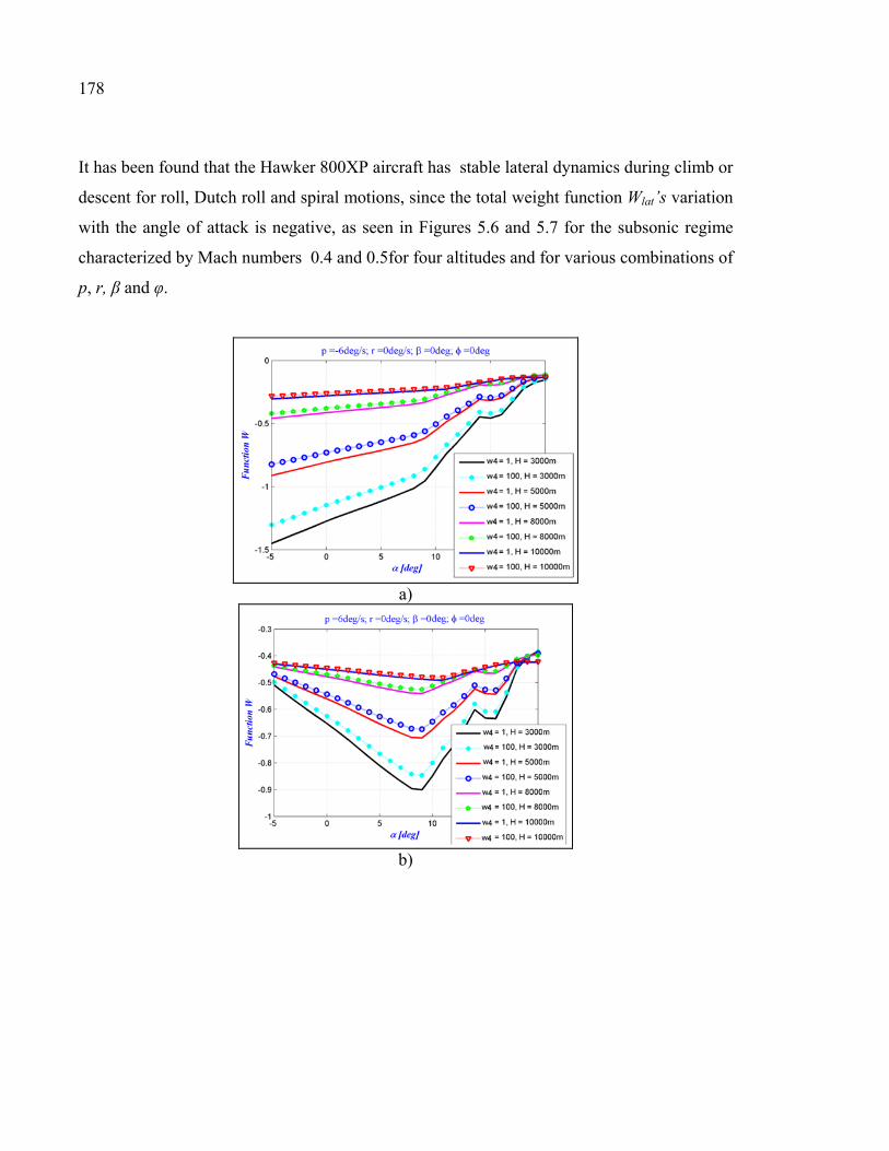
178

It has been found that the Hawker 800XP aircraft has stable lateral dynamics during climb or

descent for roll, Dutch roll and spiral motions, since the total weight function Wlat’s variation

with the angle of attack is negative, as seen in Figures 5.6 and 5.7 for the subsonic regime

characterized by Mach numbers 0.4 and 0.5for four altitudes and for various combinations of

p, r, β and φ.

a)

b)

179

c)

d)

e)

180

f)

Figure 5.7 Lateral-directional stability analysis with the WFM for different values of constant w4lat as a function of the angle of attack for M = 0.5

The stability fields for lateral motion are presented in Figures 5.6 and 5.7. We can see that

instability can occur for M = 0.4 if the limits are increased, for high angles of attack in the

cases presented in Figures 5.6a), b), and e), and for M = 0.5 for the cases presented in Figures

5.7a) and e). Meanwhile, for small angles of attack we can have stability fields if the limits

presented in Figures 5.6c), d) and f), 5.7c) and d) are increased.

The Hawker 800XP is proven to be a stable aircraft in its longitudinal and lateral motions

because the sign of the W function remains negative. The next section presents a stability

analysis using the eigenvalues method to and validate and compare the results obtained with

the WFM.

5.5 Eigenvalues stability analysis of linear small-perturbation equations

The eigenvalues stability analysis was used to validate the results obtained with the Weight

Functions Method, based on the aerodynamic coefficients and their derivatives obtained with

FDerivatives code. Five dynamic modes of motion describe the aircraft's response to an

initial condition of any origin (turbulence, control input, etc.). These five modes are: the short

period and the long period for the longitudinal aircraft motion, and the roll, Dutch roll and

spiral for the lateral motion. These modes are separated as they are defined by the equations

181

described in sections 5.5.1 and 5.5.2 for longitudinal and lateral motions, respectively. Their

estimation is made in open-loop.

5.5.1 Longitudinal motion results

The longitudinal motion can be divided into two motions: short period and phugoid. The

short period pitch response is the short answer (from 1 sec to 4 sec) of a longitudinal motion

to a disturbance, and is extremely useful to investigate. The main variables are the angle of

attack α, the load factor n and the pitch angle θ. It is interesting to find the relationships

between the damping ratio of the short period oscillation (ζsp), the undamped natural

frequency of the short period oscillation (ωsp), and the change in steady state normal

acceleration per unit change in angle of attack for incremental pitch control deflections at

constant airspeeds and Mach numbers.

The mathematical model (Hodgkinson, 1999) describing this longitudinal motion can be

represented in the form of the state space first equation (eq.(5.2)) :

0

0,

0

0 0 1 0

, ,

0

u

qu

long

quu q

long long long e

X gX

V VV ZVZ Z

V Z V Z V ZAV ZVZ M Z M

VM M M MV Z V Z V Z

X

Vu

Z

V Zx B uq

Z MM

V Z

α

α

α α α

α α αα α

α α α

δ

δ

α

δ αδ

α

αδ

θ

−

+ − − −=

+ + + + − − −

Δ Δ −= = = Δ Δ +Δ −

(5.17)

182

For both longitudinal modes, the natural frequency ωn and the damping ratio ξ are estimated

from the characteristic equation 0longI Aλ − = as functions of the eigenvalues λ1, λ2, λ3 and λ4

(eq.(5.18)), with the specification that λ1,2 correspond to short-period and λ3,4 correspond to

phugoid motions.

( )

( )( )

( )1,2 3,4

2 21,2 3,4

Re Re,

1 Im 1 Im

n n

n n

ζω λ ζω λ

ω ζ λ ω ζ λ

= =

− = − =

(5.18)

The natural frequencies ωn and the damping ξof short-period and phugoid modes verify the

next eq.(5.19).

( )( )2 2 2 22 2 0p p np np sp sp nsp nspζ ζ ω ω ζ ζ ω ω+ + + + = (5.19)

The imaginary parts of the eigenvalues are presented as functions of their real parts in Figure

5.8, where it can be observed that all the real parts of the eigenvalues are negative, which

means that, in terms of stability, the aircraft longitudinal mode is stable in both short-period

and phugoid modes. For the phugoid mode, the real parts of eigenvalues are negative, but

they are very close to positive values if the limits are increased, which means pitch angles θ

that are greater than 200 or smaller than -200 and pitch rates q less than -3.5 0/s or greater than

3.5 0/s.

183

Figure 5.8 Root locus plot (Imaginary vs. Real eigenvalues) longitudinal motion representation for M = 0.4 and 0.5

184

5.5.2 Lateral motion results

Based on eq. (5.1) and (5.2) the system can be written in the following form (Hodgkinson,

1999):

00

cos

0, ,

0

0 1 0 0

p r

xz xz xzp p r r

x x xlat lat

xz xz xzp p r r

z z z

xz

lat

YY Y V g

V V V u

I I IL N G L N G L N p

I I IA xr

I I IN L G N L G N L

I I I

Y

V

IG L N

B

G

G

β

β β

β β

δ

δ δ

θ

β

ϕ

− Δ + + + Δ = = Δ Δ+ + +

+= ,

0

x lat a

xz

z

I u

IG N L

Iδ δ

δ

= Δ + (5.20)

Generally, the eigenvalues λ1, λ2, λ3 and λ4 of the characteristic equation 0latI Aλ − =

for

lateral motion are composed of two real eigenvalues and a pair of complex eigenvalues. The

eigenvalues are chosen so that the response of the aircraft is characterized by the following

modes:

• A Spiral mode characterized by convergent or divergent motions;

• A Roll mode characterized by fast convergent motion; and

• A Dutch Roll mode characterized by lightly damped oscillatory motion with a low

frequency.

The rolling motion is generally quite damped, and reaches the steady state in a very short

time. In the case of a roll mode, the desired roll rates and angles can be obtained. The

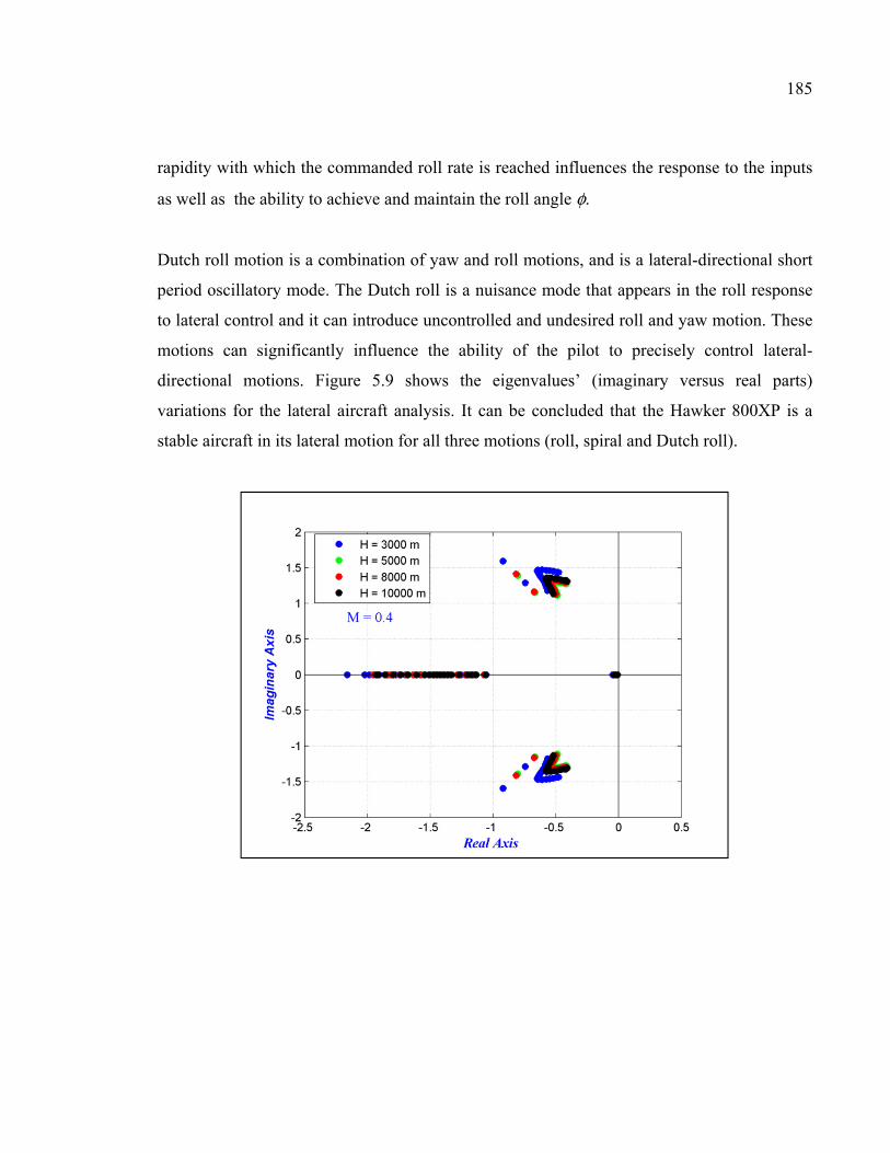
185

rapidity with which the commanded roll rate is reached influences the response to the inputs

as well as the ability to achieve and maintain the roll angle φ.

Dutch roll motion is a combination of yaw and roll motions, and is a lateral-directional short

period oscillatory mode. The Dutch roll is a nuisance mode that appears in the roll response

to lateral control and it can introduce uncontrolled and undesired roll and yaw motion. These

motions can significantly influence the ability of the pilot to precisely control lateral-

directional motions. Figure 5.9 shows the eigenvalues’ (imaginary versus real parts)

variations for the lateral aircraft analysis. It can be concluded that the Hawker 800XP is a

stable aircraft in its lateral motion for all three motions (roll, spiral and Dutch roll).

186

Figure 5.9 Root locus plot (Imaginary vs. Real eigenvalues) lateral directional motion representation for M = 0.4 and 0.5

We can see that for the highest altitude the stability field is close to instability, meaning that

any change of limits defined as roll rate p = [-6 to 6]0/s, yaw rate r = [-2 to 2]0/s, sideslip

angle β = [-5 to 5] 0 and roll angle Φ = [-15 to 15] 0 could induce instability.

5.6 Conclusions

The main objective of this study was to determine, as a design tool, the positive weight

functions by the Weight Functions Method as a means to analyze the stability fields of a

Hawker 800XP configuration. eigenvalues stability analysis of linear small-perturbation

equations was the selected validation method since eigenvalues can be determined quickly

for any flight condition as well as from the stability derivatives for a particular flight case.

The aerodynamic coefficients and their stability derivatives were found with our new in-

house FDerivatives code.

Based on the aircraft’s aerodynamic model calculated with the WFM, three functions were

defined in terms of stability derivatives terms, and the last function was considered to be

187

positive and chosen to be 1 or 100. The WFM was applied for longitudinal and lateral

motion studies.

For all four altitudes, considered at two Mach numbers, the longitudinal dynamics of the

Hawker 800XP remains stable for any combination of pitch angle/pitch rate θ/q. It was

determined that the Hawker 800XP aircraft has a stable lateral dynamic in climb or in

descent for roll, Dutch roll and spiral motions, as the total weight function W variation with

the angle of attack is negative for the subsonic regime characterized by Mach numbers 0.4

and 0.5 and at four altitudes, for combinations of p, r, β and φ.

Both methods indicate a stability field and that, for certain combinations, instability can

occur if the limits are exceeded:

• longitudinal motion at M = 0.5:

- θ smaller than -200 with q = 00/sec;

- θ smaller than -200 and q smaller than -3.50/sec

• lateral motion for high angles of attack at M = 0.4:

- p smaller than -60/s, with β = 00, r = 00/s and φ = 00 ;

- p greater than -60/s, with β = 00, r = 00/s and φ = 00 ;

• lateral motion for high angles of attack at M = 0.5:

- p smaller than -60/s, with β = 00, r = 00/s and φ = 00 ;

• lateral motion for small angles of attack at M = 0.4 :

- r smaller than -20/s, β smaller than -50 with p = 00/s and φ = 00 ;

- r greater than -20/s, β greater than -50 with p = 00/s and φ = 00;

- r smaller than -20/s or β smaller than -50 or p smaller than -60/s or φ smaller than -

150;

• lateral motion for small angles of attack at M = 0.5:

- r smaller than -20/s, β smaller than -50 with p = 00/s and φ = 00 ;

- r greater than -20/s, β greater than -50 with p = 00/s and φ = 00.


Laboratory of Research in Active Controls, Aeroservoelasticity and Avionics This article was accepted to be published in The Aeronautical Journal, Paper 3921

Résumé

Ce document évalue l'application d'une nouvelle méthode d'analyse de la stabilité du

système, la méthode des fonctions du poids, pour les mouvements longitudinaux et latéraux

d'un modèle d'aéronef qui s'appelle HIRM (High Incidence Research Aircraft Model). Le

procédé consiste à trouver le nombre de fonctions de poids qui est égal au nombre

d'équations différentielles nécessaires à la modélisation du système. La stabilité de l'aéronef

est déterminé à partir du signe de la fonction de poids total, qui doit être négatif pour un

modèle stable. Le modèle Aero-Data Model In Research Environment (ADMIRE),

développé par l'Agence suédoise de recherche pour la défense, a été utilisé pour la

modélisation aérodynamique de l'avion, avec les configurations suivantes: nombre de Mach =

0.25, altitude = 500 m, l'angle d'attaque [-10 à 30]0, angle de déflexion élevon [-30 à 30]0,

déviation canard [00 et 250] et les angles de déviation du gouvernail [-300 et 300]. Ces

configurations de vol ont été choisis parce qu'elles sont parmi les conditions de vol pour Cat.

II Oscillations Induites par le Pilote (PIO) critères de validation, effectuées sur le modèle des

avions accès à l'information présentée dans le PIO Handbook by the Group for Aeronautical

Research and Technology in Europe, Flight Mechanics/Action Group 12. Ce modèle d'avion

a une instabilité connue pour des mouvements longitudinaux et latéraux et ainsi une loi de

commande a été introduit pour stabiliser son vol.

CHAPTER 6

APPLICATION OF THE WEIGHT FUNCTIONS METHOD ON A HIGH INCIDENCE REASEARCH AIRCRAFT MODEL

190

Abstract

This paper assesses the application of a new method for system stability analysis, the weight

functions method, to the longitudinal and lateral motions of a High Incidence Research

Aircraft Model. The method consists of finding the number of weight functions that is equal

to the number of differential equations required for system modelling. The aircraft’s stability

is determined from the sign of the total weight function; which should be negative for a

stable model. The Aero-Data Model In Research Environment (ADMIRE), developed by the

Swedish Defense Research Agency, was used for the aerodynamic aircraft modelling, with

the following configurations: Mach number = 0.25, altitude = 500 m, angle of attack [-10 to

30]0, elevon deflection angle [-30 to 30]0, canard deflection [00 and 250] and rudder

deflection angles [-300 and 300]. These flight configurations were selected because they are

among the flight conditions for Cat. II Pilot Induced Oscillation (PIO) criteria validation,

performed on the FOI aircraft model presented in the PIO Handbook by the Group for

Aeronautical Research and Technology in Europe, Flight Mechanics/Action Group 12. This

aircraft model has a known instability for longitudinal and lateral motions and so a control

law was introduced to stabilize its flight.

6.1 Introduction

The Weight Function Method (WFM) has been applied in various engineering fields. For

example, it has been used to determine stress factors for crack problems. The WFM was

applied by Yoichi et al. (2003) to solve two- and three-dimensional crack problems and to

calculate stress intensity factors for arbitrary loading conditions. Their application has been

generalized to calculate the response analysis of structures and to solve two-dimensional

elasticity and plate bending problems. The weight function method was found to be useful

for analyzing structures subjected to a variety of loading conditions because the responses

expressed in terms of displacements and stresses may be calculated by integrating the inner

product of a universal weight function and a load vector. The stress intensity factor for a

191

patched crack within an infinite plate was successfully numerically validated using the WFM

(Kim et al., 2000).

Paris et al. (1976) presented an alternate method of Bueckner and Rice for the deviation of a

two-dimensional weight function to eliminate crack tip stress intensity factors. A generalised

weight function method was developed by Wu et al. (1983), based on Betti's reciprocal

theorem application to the equivalent cracks problem involving mixed boundary conditions.

Fett (1991) contributed an analytical solution for determining stress distribution using a

weight function based on the Boundary Collocation Method. Schneider et al. (1989) used a

closed-form weight function formula to calculate the stress intensity factor of an edge crack

for an elastic disc. A three-dimensional linear elastic fracture mechanics (LEFM) problem

was also solved using the WFM (Vainshtok et al., 1987).

Stroe (2008) solved the Lurie-Postnikov problem using general vibration equations involving

linear transformations. Stroe also analyzed a holonomic system with dependent variable

equations in (Stroe et al., 2008), where the WFM was applied to vibration and stability

studies in cases of damped holonomic systems.

The selections of H∞ weighting functions were presented for practical applications by

Jiankun et al. (2000), where the authors showed that an H∞ weighting function for a single-

input single-output system could be obtained by considering it as a series of connections of

elementary low-order systems. For a constrained control effort, an explicit weighting

function was obtained. They proposed a novel method for the selection of weighting

functions in an H∞ mixed sensitivity design to directly control the percentage overshoot.

Real-time experimental results were presented for the roll-angle control of a laboratory scale

model of a vertical take-off aircraft (Jiankun et al., 2000).

Our analysis of longitudinal and lateral motions using the WFM was performed on the Aero-

Data Model In Research Environment model (ADMIRE) developed by the FOI

(Admirer4p1), based on the Generic Aerodata Model (GAM) developed by SAAB AB in the

framework of the GARTEUR Group (GARTEUR FM(AG12), 2001). « The ADMIRE

192

describes a generic small-single seated, single-engine fighter aircraft with a delta-canard

configuration, implemented in MATLAB/SIMULINK Release 13 » (Lars et al., 2005, pp iii).

The stability domains were determined for each flight case for the given configurations.

This paper is part of a project developed at LARCASE laboratory to perform a more

complete analysis of an aircraft in subsonic regime as a design tool, based on geometrical

parameters. Three real different configurations were analyzed and HIRM model was chosen

for its instability well known. The WFM was applied to the original non-linear aerodynamics

model implemented in ADMIRE simulation, as well as for the model stabilized with control

laws, in order to stabilize its flight.

6.2 The HIRM: Model Description and its Implementation in Admire Code

The HIRM (High Incidence Research Model) (Admirer4p1), (Lars et al., 2005), (Terlouw,

1996) of a generic fighter aircraft was used in this study. This aircraft model has an envelope

defined by a Mach number between 0.15 and 0.5 and altitude of between 100 and 20,000 ft

for the following angles: the angle of attack α = [-10 to 30] degrees, sideslip angle β = [-10

to 10] degrees, elevon angle δe = [-30 to 30] degrees, canard angle δc = [-55 to 25] degrees,

and rudder angle δr = [-30 to 30] degrees.

The aerodynamics coefficients were obtained based on wind tunnel and flight tests for a

model « ... originally designed to investigate flight at high angles of attack ... but [that] does

not include compressibility effects resulting from high subsonic speeds. » (Terlouw, 1996, p

21). These coefficients were further implemented in the ADMIRE model using the main

graphical window simulation presented in Figure 5.1, which also shows the response of the

aircraft model. The tests and analyses provided in the GARTEUR program were focused on

PIO detection, while this paper evaluates a new method to investigate the model’s stability.

« The ADMIRE contains twelve states (VT, α, β, pb, qb, rb, ψ, θ, φ, xv, yv, zv) plus additional states due to actuators and Flight Control System (FCS). Available control effectors are left- and right canard, leading edge flap, four elevons, rudder and

193

throttle setting. The model is also equipped with thrust vectoring capability and an extendable landing gear. The model is prepared for the use of atmospheric turbulence as external disturbance. The ADMIRE is augmented with an FCS in order to provide stability and sufficient handling qualities within the operational envelope (altitude <6 km, Mach < 1.2). The FCS contains a longitudinal and a lateral part. ... The lateral controller enables the pilot to perform roll control where the roll motion is initiated around the velocity vector of the a/c, and angle of sideslip control. Sensor models are incorporated. The 20 ms flight computer delay on the actuator inputs that is implemented in other versions of ADMIRE was not used here. The model has the facility to define model uncertainties, but this was not used. ADMIRE is implemented in MATLAB and SIMULINK using a combination of standard SIMULINK blocks and S-functions written in C. » (GARTEUR FM(AG12), 2001, p 36).

Figure 6.1 is a screenshot of the ADMIRE window simulation and it is presented here to

understand how this model works. Each block is define on different level and for Aircraft

Response a screen shot was considered necessary, because of the ADMIRE_main block

which contains the non-linear coefficients given as tables.

194

Figure 6.1 ADMIRE: Main graphical window simulation and Aircraft response Source: Screenshot from graphical interface (Admirer4p1)

195

The following table contains a summary of the aircraft geometrical data, along with aircraft

mass and mass distribution data (Lars et al., 2005).

Table 6.1 HIRM geometrical data

Parameters Numerical values [Units] Wing area S 45 m2

Wing span b 10 mWing Mean Aerodynamic Chord c 5.2 m

Mass m 9100 kgx-body axis moment of inertia Ix 21000 kgm2

y-body axis moment of inertia Iy 81000 kgm2

z-body axis moment of inertia Iz 101000 kgm2

xz-body axis product of inertia Ixz 2500 kgm2

zeng -0.15 mxcg 0.25 c

Let us consider a model defined by a nonlinear autonomous system of equations for the

longitudinal motion and for its lateral motion, given below as (6.1) and (6.2), respectively

(Lars et al., 2005), (Terlouw, 1996), (Schmidt, 1998).

[ ]

1cos sin

1sin cos

1

D

L

m CG T ey

qSV C T g

m mqS g

C T mmV mV V

q qScC x qSC z TI

q

α γ

γ α γ

θ

= − + − = + − = + + =

(6.1)

( )

( ) ( )

cos

1

1

y

z y lx

y x n cg yz

qS gp r C sin

mV V

p I I qr qSbCI

r I I pq qS cC x CI

p

β α φ θ

φ

= − − + = − − +

= − − + − =

(6.2)

196

The aerodynamic force and moment coefficients contain degrees of non-linearities, as shown

in the next eq.(6.3). Their values were obtained from the ADMIRE simulation

(Admirere4p1):

( ) ( ) ( ) ( )( ) ( ) ( )( ) ( ) ( ) ( ) ( )

( ) ( )

( ) ( ) ( ) ( ) ( )

1 2 3 4

1 2 3

1 2 3 4 5

6 7

1 2 3 4 5

, , , ,

, ,

, , ,

, , ,

sin cos

cos sin

, , , , ,

N N N e N c N e

T T T e T c

m m m e m c m m c

m c m a

D N T

L N T

y y y r y a y ca y

C C C C C

C C C C

C C C C C C q

C C

C C C

C C C

C C C C C C p

α α δ α δ α β δα α δ α δ

α α δ α δ α α α δ

α β δ α δα αα α

α β α β δ α δ α δ α β

= + + +

= + + = + + + + +

+ +

= + = −

= + + + +

( )( ) ( ) ( ) ( ) ( ) ( )( ) ( ) ( ) ( ) ( ) ( )

6

1 2 3 4 5 6

1 2 3 4 5 6

,

, , , , , , ,

, , , , , , , ,

y

l l l r l a l c ca l l

n n n r n a n c ca n n

C r

C C C C C C p C r

C C C C C C p C r

α β

α β α β δ α δ α δ δ α β α β

α β α β δ α β δ α δ δ α β α β

+ = + + + + +

= + + + + + (6.3)

6.3 The Weight Functions Method

The main objective of this paper is to study, based on the above eq.(6.1) and (6.3), the HIRM

stability when the Weight Function Method (WFM ) is applied. The WFM is based on the

following theorem:

Theorem (Stroe et al., 2008): Given the autonomous system ( ) , nx f x x R= ∈ , if wk (x1, x2...

xn) exists such that 1

n

k k kk

dV x w dx=

= is a total exact differential, then its stability is given by

1

n

k k kk

W x w f−

= as follows:

• if W is negative-definite, the solution is asymptotically stable;

• if W is the null function, the solution is neutrally stable; or

• if W is positive-definite, the solution is unstable.

197

The WFM replaces the classical Lyapunov function by finding a problem with a method

which obtains a number of weight functions equal to the number of the first-order differential

equations modelling the system (Stroe, 2008), (Stroe et al., 2008). The difference between

these two methods is that the weight functions method finds one function at a time, with their

number equal to the number of the first-order differential equations.

The WFM’s basic principle is to find three positive weight functions for a system with four

first-order differential equations, where the fourth weight function is a constant, imposed by

the author. The total weight function 4

1k k k

k

W w x f=

= is defined, and its sign should be

negative to ensure the stability of the aircraft.

6.3.1 Longitudinal aircraft model

For longitudinal aircraft modeling, it was assumed that 0, andV const h constγ = = = ; with

these conditions, the first two equations of eq.(6.1) become equivalent to

( )sin cos sin sinD L TT mg qS C C mg qSCα α α α= + − = + (6.4)

and the longitudinal model is described by .

( ) ( ) ( ) ( )( )

( ) ( ) ( ) ( ) ( )( ) ( )

( )

1 2 3

1 2 3 4 5

6 7

1 2

, , sin

, , ,

, , ,

or

sin

cg e T T e T c ey

m m e m c m m c

y m c m a

M cg e T e My y

q

qS mgq x z C C C z

I qS

C C C C C qqSc

I C C

q

qS mg qSq cC x z C z cC q

I qS I

α

α α δ α δ α

α α δ α δ α α α δ

α β δ α δ

α

α

= = + + + + +

+ + + + + + + +

=

= + + + +

(6.5)

where CM1 is the sum of Cm1, Cm2, Cm3, Cm6 and Cm7 , and CM2 = Cm4 + Cm5.

198

The total weight function Wlong is given by eq.(6.6), where 1 2,f f qα= = :

( )

( ) ( )( )

2

1 1 2 21

1 2 1 2

1 2 2 1 2

sin

sin

long k k k long longk

long long M cg e T e My y

long long e long M M cg e Ty y

W w x f w f w qf

qS mg qSw q w q cC x z C z cC q

I qS I

mg qSq w w z w q c C C q x z C

I I

α

α α

ααα

=

= = + =

= + + + + + =

= + + + + +

(6.6)

In the first parenthesis of eq.(6.6) that multiplies the term αq, the first weight function wlong1

is defined as 1 2

sin0long long e

y

mgw w z

I

αα

= − > , for any positive value of wlong2, because ze = -

0.15 m is negative from the aircraft geometry, a value implemented in the ADMIRE

simulation.

The next step consists of replacing wlong1 in eq.(6.6) and obtaining the total longitudinal

weight function Wlong , as defined in eq.(6.7), where its sign depends on the sign of q.

( ) ( )( )2 1 2long long M M cg e Ty

qSW w q c C C q x z C

I

= + + +

(6.7)

6.3.2 Lateral aircraft model

The lateral model was given in eq.(6.2), and using the following notations: ( )

1z y

x

I Ii I

−= ,

( )3

y x

z

I Ii I

−= , eq. (6.2) is written in the form:

199

( ) ( )( ) ( ) ( )

( ) ( )

1

3

1

3

or

1a r

r a a

r a a

y

lx

n cg yz

p r a r

p r r a

p p r r a

qSp r C

mVqSb

p i qr CI

qSr i pq cC x C

I

p

y y p y r y y

p l l l p l i q r l l l

r n n n i q p n r n n n

p

β δ δ

β αβ δ δ αδ

β α δ δ αδ

β α

φ

β β α δ δ

α β δ α δ

β α δ α δ

φ

= − − = − +

= − + − = = + + + − + + = + + + − + + + = + + + + + + +

=

(6.8)

The system of eq.(6.8) can be simplified as follows:

1

2

3

4

a r

r a

r a

p r a r

p r r a

p r r a

f y Y p Y r y y

f L l p L r l L

f n N p n r n N

f p

β δ δ

β δ δ

β δ δ

β δ δβ δ δβ δ δ

= + + + + = + + + +

= + + + + =

(6.9)

where 1 2 3 4, , ,f f p f r fβ φ= = = = , and

( ) ( )( ) ( ) ( )( ) ( )

1

3

, 1

, ,

,

a a a

a a a

p p r r

r r

p p p

Y y Y y

L l l L l i q L l l

N n n i q N n n

β β αβ δ δ αδ

α δ δ αδ

α

α α

α α

= + = −

= + = − = +

= + + = +

(6.10)

By denoting the state vector [ ] ,T

kx p rβ φ= the lateral weighting function is then given

as:

( ) ( )( )

( )

4

1 1 2 2 3 3 4 41

1 2

3 4

1 3

a r r a

r a

r a

lat latk k k lat lat lat latk

lat p r a r lat p r r a

lat p r r a lat

lat lat r lat p r r a

W w x f w f w pf w rf w f

w y Y p Y r y y w p L l p L r l L

w r n N p n r n N w p

W w Y w N p n r n N r

β δ δ β δ δ

β δ δ

δ δ

β φ

β β δ δ β δ δ

β δ δ φ

β δ δ β

=

= = + + + =

= + + + + + + + + + +

+ + + + + +

= + + + + +

( )( ) ( )

1 3

1 2 4a r r a

lat lat

lat p a r lat p r r a lat

w y w n r

w Y p y y w p L l p L r l L w p

β β

δ δ β δ δ

β

β δ δ β δ δ φ

+ +

+ + + + + + + + +

(6.11)

200

To solve the stability analysis problem, the first weight function is defined from the third

term of the lateral weighting function, eq.(6.11), where wlat3 is a constant defined by the

authors as equal to 1 in this paper, so that:

1 3lat lat

n rw w

yβ

β β= − (6.12)

Equation (6.12) is replaced in eq.(6.11), to obtain:

( )

( ) ( )

3 2 4

3 2

2 3

a r

r a r a

lat lat p p lat p lat

lat r a r lat r

lat r a lat r r a

nW w r N Y w l p w p

y

nw Y r y y w L p r

y

w p L l L w n r n N r

β

β

βδ δ

β

β δ δ δ δ

φ

δ δ

β δ δ δ δ

= − + + +

+ − + + + +

+ + + + + +

(6.13)

The second weight function, wlat2 , can be defined as a function of the wlat3 positive function:

( )2 3 a rlat lat r a rr

nw w Y r y y

y L pβ

δ δβ

δ δ= + + (6.14)

The last step in our analysis is to find the total Wlat lateral weight function, defined in

eq.(6.15), so that the wlat4 function can be given in eq.(6.16) as a function of wlat3.

( )

( )( )

( )

3 4

3

a r

a r r a

r a

plat lat a r lat

r

r a r r ar

lat

pr r a p p

r

n lW w y y w p

y L r

nY y y L l L

y Lw

lnn r n N r N rp p Y

y L r

βδ δ

β

βδ δ β δ δ

β

βδ δ

β

δ δ φ

δ δ β δ δ

δ δ

= + + +

+ + + + +

+ + + + + −

(6.15)

( )4 3 a r

plat lat a r

r

n lw w y y

y L rβ

δ δβ

δ δφ

= − + (6.16)

Finally, the final weight function Wlat is determined from wlat1, wlat2 and wlat4 , given by

eq.(6.12), (6.14) and (6.16) as a functionof wlat3,

201

( )( )

( )3

a r r a

r a

r a r r ar

lat lat

pr r a p p

r

nY y y L l L

y LW w

lnn r n N N p r p Y

y L r

βδ δ β δ δ

β

βδ δ

β

δ δ β δ δ

δ δ

+ + + + +

= + + + + + −

(6.17)

6.4 Results

The longitudinal motion's results are presented for a range of angles of attack, elevon angles

and canard angles defined as α = [-10 to 30]0, δe = [-30 to 30]0 , δc = 00, and sideslip angle β

= 20 . For the lateral motion, the roll rate p = [–10 to 10]0/s, the yaw rate r = [–5 to 5]0/s, the

sideslip rate β = [0 to 10]0 and the bank angle Φ = [–20 to 20]0.

The system defined by eq.(6.1) and (6.2) is linearized about a specific equilibrium point, and

the results are presented for longitudinal and lateral motions with and without control laws in

Figures 6.5 and 6.8, respectively. In this context, investigations based on the HIRM database

and using the WFM have shown the stability and instability fields and the simple stable

solutions for the different system configurations.

6.4.1 Longitudinal motion

An analysis of the mathematical model was performed, based on the weight function wlong1

given by eq. (6.6) and with wlong2 positively defined. The results are for a system with Mach

number M = 0.25, an altitude of 500 m, a null canard angle, sideslip angle β = 10, and for the

same variation of angle of attack and elevon deflection as presented for the equilibrium

solution.

In this case, based on eq. (6.7), a dependence on the sign of q can be observed. The weight

function wlon2 is equal to 1, the smallest integer. The variation of the total weight function W

versus the angle of attack and elevon deflection are given in Figure 6.2 (a) for negative

values, q = -5 0/s and in Figure 6.2 (b) for positive values, q = 5 0/s. The sign of q changes

202

when the stability field is unstable, and vice versa. The aircraft is simple stable for the pairs

of angle of attack and elevator angle given in Figure 6.3.

a)

b)

Figure 6.2 Total weight function W for a complete range angle of attack/elevon deflection, with a null canard deflection for longitudinal motion.

203

Figure 6.3 Stability/instability fields for longitudinal motion using the Weight Functions Method with w2 = 1

The simple stable solution varies between (α = -100, δe = -140) and (α = 25.40, δe = 29.930), as

shown in Figure 6.3.

The two equilibrium curves for elevon and canard deflection angles versus angle of attack are

shown in Figure 6.4, for an altitude of 500 m and Mach number M = 0.25. The symmetrical

elevon deflection angle was estimated using eq.(6.18) and (6.19):

_ _

_ _

,2

ei lie in rie inei eye

ey loe in roe in

δ δ δδ δδ

δ δ δ= +− = = + (6.18)

where :

_

_

_

_

left outboard elevon angle

right outboard elevon angle

left inboard elevon angle

right inboard elevon angle

lie in

rie in

loe in

roe in

δδδδ

−

−

−

−

(6.19)

204

Figure 6.4 Equilibrium curves for elevon and canard deflection angles versus angle of attack

The total weight function variation with α for the longitudinal motion, for wlong2 = 1, is given

by eq.(6.7) and is shown in Figure 6.5. The smallest integer 1 was used for wlong2 ,which

multiplies a term whose sign is analyzed here (w1), so that for any higher value of the

constant wlong2, the variation of W is the same only its value increases. The red curve shows

the variation of the total weight function with α in Figure 6.5, where it can be seen that for:

• α = [-100 ÷ 10.87760) and δe = (-40 ÷ 3.5850) the aircraft is asymptotically stable;

• α = 10.87760 and δe = 3.5850 the aircraft is simple stable;

• α = (10.87760 ÷300] and δe = (3.5850 ÷ 190) the aircraft is unstable;

205

Figure 6.5 Weight function W without/ with a control law at equilibrium for longitudinal motion

To stabilize the model, a control law was used for the longitudinal aircraft motion, given by:

0e e qk k qαδ δ α= + + (6.20)

Using this control law with the regulator gains kα = 0.4 and kq = 1.284 (Admirer4p1), the

stability field increases, as shown by the total weight function W, represented by the green

curve in Figure 6.5. In order to analyze aircraft's stability as function of α and δe, the value of

δe at equilibrium corresponding to the angle of attack α was obtained from Figure 6.4. It was

concluded that, with aircraft longitudinal motion, for:

• α = (-0.640 ÷ 300] and δe = (-1.0630 ÷ 260) the aircraft is asymptotically stable;

• α = -0.640 and δe = -1.0630 the aircraft is simple stable;

• α = [-100 ÷ -0.640] and δe = (-100 ÷ -1.0630) the aircraft is unstable.

206

6.4.2 Lateral motion

Based on the weight functions wlat1, wlat2 and wlat4 given in eq.(6.12), (6.14), (6.16) and with

wlat3 positively defined by the authors, results are presented for a Mach number M = 0.25,

altitude H = 500 m, sideslip angle β = 20, roll rate p = [–10 to 10]0/s, yaw rate r = [–5 to 5]0/s,

bank angle Φ = [–20 to 20]0 , and the same variation of angle of attack and elevon deflection

presented for longitudinal motion in this paper. The sign of eq.(6.17) depends on the signs of

p, r and ɸ.

The weight function wlat3 has the same value as that of the longitudinal motion, the smallest

integer equal to 1, and the variations of the total weight function W versus angle of attack and

elevon deflection are given in Figure 6.6 ((a) for negative value p = -100/s, r = -50/s, Φ = -200

, (b) for null values p = 00/s, r = 00/s, Φ = 00 and (c) for positive values p = 100/s, r = 50/s, Φ

= 200). Figure 6.6 (b) is a section with the plane, i.e. W =0.

a)

207

b)

c)

Figure 6.6 Total weight function W for a complete range of angle of attack/elevon deflection, for lateral motion

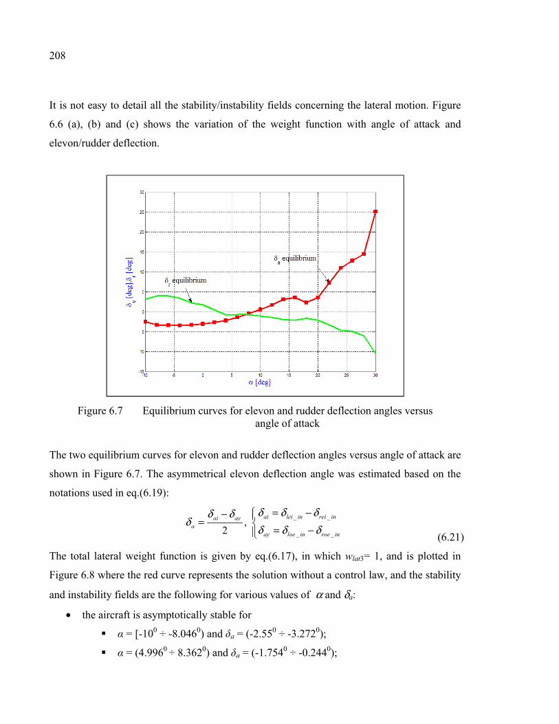
208

It is not easy to detail all the stability/instability fields concerning the lateral motion. Figure

6.6 (a), (b) and (c) shows the variation of the weight function with angle of attack and

elevon/rudder deflection.

Figure 6.7 Equilibrium curves for elevon and rudder deflection angles versus angle of attack

The two equilibrium curves for elevon and rudder deflection angles versus angle of attack are

shown in Figure 6.7. The asymmetrical elevon deflection angle was estimated based on the

notations used in eq.(6.19):

_ _

_ _

,2

ai lei in rei inai aya

ay loe in roe in

δ δ δδ δδ

δ δ δ= −− = = − (6.21)

The total lateral weight function is given by eq.(6.17), in which wlat3= 1, and is plotted in

Figure 6.8 where the red curve represents the solution without a control law, and the stability

and instability fields are the following for various values of α and δa:

• the aircraft is asymptotically stable for

α = [-100 ÷ -8.0460) and δa = (-2.550 ÷ -3.2720);

α = (4.9960 ÷ 8.3620) and δa = (-1.7540 ÷ -0.2440);

209

α = (12.290 ÷ 19.3890) and δa = (1.9240 ÷ 3.2010);

α = (22.970 ÷ 300) and δa = (9.070 ÷ 25.150);

• the aircraft is simple stable for:

α = -8.0460 and δa = -3.2720 ;

α = 4.9960 and δa = -1.7540 / α = 8.3620 and δa =-0.244 0;

α = 12.290 and δa = 1.9240 / α = 19.389 and δa = 3.2010;

α = 22.970 and δa = 9.070;

• the aircraft is unstable for:

α = (-8.0460 ÷ 4.9960) and δa = (-3.2720 ÷ -1.7540);

α = (8.3620 ÷ 12.290) and δa = (-0.2440 ÷ 1.9240);

α = (19.3890 ÷ 22.97) and δa = (3.2010 ÷ 9.070);

A control law was used to stabilize the model, given by:

0

0

a a p

r r

k p k

k k

φ

β β

δ δ φ

δ δ β β

= + +

= + +

(6.22)

Figure 6.8 Weight function W with and without a control law at equilibrium for lateral motion

210

This control law was used with the regulator gains given as kp = 0.52106, kφ = -0.27704, kβ =

7.6727, and kβdot = -4.9301 (Admirer4p1); the field of stability increases for the range of

angles of attack from -10 to 15.67 degrees (see the blue curve in Figure 5.8), as shown next

for different values of α and δa:

• asymptotically stable for:

α = (-100 ÷ 15.670) and δa = (-2.5510 ÷ 3.470)

α = (19.450 ÷ 20.730) and δa = (3.1860 ÷ 4.8940)

α = (23.210 ÷ 300) and δa = (9.7120 ÷ 25.150);

• simple stable for:

α = 15.670 and δa = 3.470;

α = 19.450 and δa = 3.1860;

α = 20.730 and δa = 4.8940;

α = 23.310 and δa = 9.7120;

• unstable for:

α = (15.670 ÷ 19.450) and δa = (3.470 ÷ 3.1860) ;

α = (20.730 ÷ 23.210) and δa = (4.8940 ÷ 9.7120).

6.5 Conclusions

The maneuverability of an aircraft is determined by its ability to change its attitude and speed

about three axes (longitudinal, lateral and vertical). The main aim of this paper was to

determine the positive weight functions by using the Weight Functions Method to analyze

the stability/instability fields of an HIRM model and to stabilize this model using control

laws.

For the autonomous system of differential equations used in this paper, the WFM gives the

stability and instability fields. Based on the analysis presented above for the nonlinear model,

the oscillatory behavior was observed for the lateral motion, equivalent to an unstable one,

and for longitudinal motion it could be seen that the sign of q changes the stability field to

unstable and vice versa.

211

The HIRM is an unstable model and the control law introduced for each motion, longitudinal

and lateral, was used to stabilize its flight in the range of α = (-0.640 ÷ 300] and δe = (-1.0630

÷ 260) for longitudinal motion, and α = (-100 ÷ 15.670) and δa = (-2.5510 ÷ 3.470) for lateral

motion.

GENERAL CONCLUSION

In this thesis, a new code FDerivatives was used to determine the aerodynamic coefficients

and their derivatives. Utilizing those derivatives, a new method, called the Weight Functions

Method, was applied for stability analysis of three aircrafts. In addition, a continuity

algorithm was used to define the minimum airspeed of flight envelope. The main

contribution of this thesis consisted on the application of these approaches to define a new

stability analysis design tool, a lower cost paid to defined the stability fields for an aircraft

versus a CFD method.

Based on the DATCOM method and using the geometrical parameters of two real aircraft as

input, a new code called FDerivatives was developed at the LARCASE laboratory.

FDerivatives is an in-house code developed for the subsonic regime for classical Wing-

Body-Tail configurations and applied on the Hawker 800XP aircraft and a delta-wing

configuration, tested on X-31 aircraft. The work developed and validated for the X-31 was

part of a major project funded by NATO in the framework of NATO RTO AVT–161 «

Assessment of Stability and Control Prediction Methods for NATO Air and Sea Vehicles »,

This project was awarded with the « RTO Scientific Achievement Award 2012 »,that is the

most prestigious award given to NATO’s AVT-161 research team .

Compared to the applicability limits of the Digital DATCOM, the FDerivatives code adds

several enhancements by taking into account a smaller number of the geometrical parameters

of an airplane, with the fuselage modeled as a body of revolution and using the real airfoil

coordinates. In the new code, the calculation possibilities have been extended to wings with

variable airfoils along the span and with negative sweepback. Different approaches to

calculate the drag and pitching moment must still refine the results for the drag coefficient

and to significantly improve those of the coefficient of pitching moment. Presagis gave the «

Best Simulation Award » to the LARCASE laboratory for FDerivatives and data FLSIM

applications.

214

The results for both aircraft are presented in Chapter 2 and in Chapter 3, validated with flight

test data provided by CAE Inc. for Hawker 800XP business aircraft and with the

experimental data provided in the Low–Speed Wind Tunnel of the German–Dutch Wind

Tunnels (DNW–NWB) for the X–31 model.

Proper geometric modelling is essential to correctly obtain aerodynamic coefficients and

their derivatives. Pitching moment coefficient analysis demonstrated how a correct

approximation of an aircraft’s geometry can be obtained. Lift, drag and pitching moment

coefficients, for angles of attack between –2 and 20 degrees, were calculated with very good

accuracy by the FDerivatives code. In addition, rolling and yawing moment coefficients and

side force coefficients were well–estimated.

The weight functions method (WFM) was chosen as the means to study the airplane's

stability for longitudinal and lateral motions. This new method determines a number of

weight functions that are equal to the number of first-order differential equations. The WFM

was selected because this thesis serves as a summary of the code(s) and methods needed to

perform a complete aircraft analysis at the design phase, based only on its geometrical

parameters. A stability analysis based on the null solutions stability studies for differential

equation systems was presented in Chapters 4, 5 and 6. The main aim was to find the positive

weight functions in order to analyze aircraft stability, considering the negative sign of the

total weight function. Hawker 800XP and X-31 aircraft were determined to be stable for the

configurations considered. The weight functions method was validated with the root locus

method.

A third model was analyzed to validate the new method and the continuity algorithm. The

High Incidence Research Aircraft Model (HIRM) developed by the Swedish Defense

Research Agency and implemented in Aero-Data Model In Research Environment

(ADMIRE) code was chosen because it is known to be an instable model. Its stability and

instability fields have been determined, as well as an equilibrium configuration for

215

longitudinal and lateral motions. Control laws, introduced in Chapter 5, were utilized to

stabilize the aircraft and to determine the new stability fields.

These fields are for:

• angle of attack α = (-0.640 ÷ 300] and elevon angle δe = (-1.0630 ÷ 260) for

longitudinal motion; and

• angle of attack α = (-100 ÷ 15.670) and aileron angle δa = (-2.5510 ÷ 3.470) for lateral

motion.

The continuity algorithm was presented in Section 0.6. This method was used to define the

new minimum airspeeds of the flight envelope for the HIRM model stabilized with a control

laws and validated with numerical results. The initial conditions were calculated for three

Mach number/Altitude pairs: (M = 0.22, H = 20m), (M = 0.22, H = 3000m) and (M = 0.55, H

= 6000m). For smaller Mach numbers and altitudes less than or equal to 3000 m we have

improved the flight envelope, up to Mach number M = 0.182. For altitudes values situated

between 3000 m and 6000 m the flight envelope the improvement was considerable.

The most important steps of this thesis are found in the journal publications as follows:

• The development and use of a new code, FDerivatives, to estimate aerodynamic

coefficients and their derivatives, based on the geometrical parameters presented in

the first two papers;

• The identification and use of the weight functions method for the longitudinal and

lateral stability of three real aircraft in the third, fourth and fifth papers;

• The continuity algorithm presented in section 0.6.

RECOMMANDATIONS

The research presented in this thesis could be improved in many ways or be used as a starting

point to undertake many other research projects:

1. Complete the FDerivatives code with the stability derivatives related to control

surfaces;

2. The weight functions defined for a typical aircraft configuration could be further

generalized by use of new similar configurations. The Weigh Function Method was

never used for aircrafts stability and for this reason a general model can be useful. It

would be suitable to keep or modify and validate this method with the aim of model

generalization;

3. Define a new code to implement all methods and the code FDerivatives presented in

this thesis into a single code, based only on the geometrical parameters of an aircraft,

completed by the airfoils coordinates.

APPENDIX A: GEOMETRICAL PARAMETERS OF THE AIRCRAFT

PRESENTED IN REFERENCE NACA-TN-4077

Fuselage

Length, [ft] 3.750

Finesse ratio 7.50

Mounting point, distance measured from nose of fuselage parallel to the fuselage

reference line, [ft]

2.125

Diameter at c/4 of tail group, [ft] 0.170

Vertical tail

Aspect ratio 1.4

Sweep angle of quarter-chord line, [deg] 45

Taper ratio 0.6

Span, [ft] 0.688

Root chord, [ft] 0.614

Tip chord, [ft] 0.368

Mean aerodynamic chord, cV, [ft] 0.502

xV, [ft] 0.468

zV, [ft] 0.315

Area ratio, SV / SW 0.15

NACA airfoil section in planes parallel to the fuselage centre line 65A008

Horizontal tail

Aspect ratio 2.77

Sweep angle of quarter-chord line, [deg] 45

Taper ratio 0.60

Span, [ft] 1.117

Root Chord, [ft] 0.504


Mean aerodynamic chord, cH, [ft] 0.412

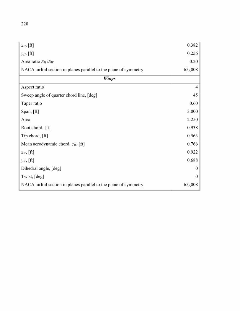
220

xH, [ft] 0.382

yH, [ft] 0.256

Area ratio SH /SW 0.20

NACA airfoil section in planes parallel to the plane of symmetry 65A008

Wings

Aspect ratio 4

Sweep angle of quarter chord line, [deg] 45

Taper ratio 0.60

Span, [ft] 3.000

Area 2.250

Root chord, [ft] 0.938


Mean aerodynamic chord, cW, [ft] 0.766

xW, [ft] 0.922

yW, [ft] 0.688

Dihedral angle, [deg] 0

Twist, [deg] 0

NACA airfoil section in planes parallel to the plane of symmetry 65A008

APPENDIX B: LONGITUDINAL AND LATERAL AERODYNAMIC DERIVATIVES

The non-dimensional aerodynamic derivatives for conventional aircraft are next presented, divided

into two groups, longitudinal and lateral (Schmidt, 1998).

There are three categories of derivatives: static, dynamic and control.

• Static derivatives include all those derivatives concerned with the angle of attack α and

the sideslip angle β; they give the force and moment variations with respect to changes in

the aircraft position.

• Dynamic derivatives include the force and moment derivatives, with respect to time, of

the change of angle of attack α, of sideslip angle β and of roll rate p, pitch rate q and yaw

rate r.

• Control derivatives result from the control actuation.

B.1 Longitudinal parameters

Short-period derivatives

Heavy damping lift curve slope

( )w D L

Z qSZ C C

V mVα

α= = − +%

Longitudinal static stability

my

qScM C

Iα α=%

Pitch damping /pitching moment due to pitch rate

2q mqy

qSc cM C

I V=

%

Pitching moment due to angle of attack rate

2 my

qSc cM C

I Vα α=& &

%

Phugoid derivatives

Phugoid damping parameters

222

2u D

qSX C

mV= −

%

Vertical speed stiffness parameters

2u L

qSZ C

mV= −

%

B.2 Lateral directional derivatives

Roll mode derivatives

Roll damping

2p lpx

qSb bL C

I V =

%

Lateral control effectiveness

a l ax

qSbL C

Iδ δ=%

Dutch roll derivatives

The weathercock

nz

N qSbN C

V VIβ

ν β= =%

Yaw damping

2r nrz

qSb bN C

I V =

%

Side force due to velocity

y

qSY C

mν β=%

The directional control

r n rz

qSbN C

Iδ δ=%

223

Lateral-directional cross derivatives

Dihedral effect

lx

L qSbL C

V VIβ

ν β= = %

Rolling due to yawing

2r lrx

qSb bL C

I V =

%

Yawing due to rolling

2p npz

qSb bN C

I V =

%

BIBLIOGRAPHY

Abbot, Ira H. and A.E. von Doenhoff. 1959. Theory of wing sections, Including a Summary of Airfoil Data, New York: Dover Publication Inc.

Admirer4p1. Online < http://www.foi.se/en/Our-Knowledge/Aeronautics Admire/ Downloads >. Verified March, 29 2013. Advanced Aircraft Analysis 3.3 code. Online < http://www.darcorp.com/Software/AAA/ >.

Verified April, 04 2013. Alley, N.R., Phillips, W.F. and Spall, R.E. 2007. « Predicting Maximum Lift Coefficient for

Twisted Wings Using Computational Fluid Dynamics ». Journal of Aircraft, Vo.44, No 3.

Anscombe, A. and Raney, D.J. 1950. Low-speed tunnel investigation of the effect of the body

on Cm0 and aerodynamic centre of unswept wing-body combinations. (ARC)/CP-16, Aeronautical Research Council.

Anton, Nicoleta. 2005. « Analiza miscarii longitudinale a unui avion de mare manevrabilitate

prin metoda bifurcatie ». “AEROSPACE 2005” Conference, October 11–12, Bucharest.

Anton, Nicoleta, Botez, Ruxandra Mihaela and Popescu, Dumitru. 2011. « Stability

derivatives for X-31 delta-wing aircraft validated using wind tunnel test data ». Proceeding of the Institution of Mechanical Engineers, Vol. 225, Part G, Journal of Aerospace Engineering, pp 403-416.

Anton, Nicoleta, Botez, Ruxandra Mihaela and Popescu, Dumitru. 2010. « New

methodology and code for Hawker 800XP aircraft stability derivatives calculations from geometrical data ». The Aeronautical Journal, Vol. 114, No. 1156, Paper No. 3454.

Anton, Nicoleta, Botez, Ruxandra Mihaela and Popescu, Dumitru. August 10-13, 2009. «

New methodologies for aircraft stability derivatives determination from its geometrical data ». AIAA Atmospheric Flight Mechanics Conference. AIAA 2009-6064, Chicago, Illinois.

Babcock, D.A. and A.S. Arena Jr., 2004. « Estimating Aircraft Stability Derivatives through

Finite Element Analysis ». AIAA 2004–5174. Bihrle, W. 1965. A Handling Qualities Theory for Precise Flight Path Control, Tech. Rep.

AFFDL-TR-65-195, AFRL, Wright Patterson AFB, OH.

226

Blake, William B. and Etan D. Karni. June, 2005. « A Cambered Body Method for Missile DATCOM ». 23rd AIAA Applied Aerodynamics Conference, Toronto, Ontario Canada. p. 11.

Boelens, O.J. June 22 – 25, 2009. « CFD Analysis of the Flow around the X-31 Aircraft at

High Angle of Attack ». 27th AIAA Applied Aerodynamics Conference. AIAA 2009–3628–968, San Antonio, Texas.

Botez, Ruxandra. 2004. Notes de cours GPA740: Système informatique embarqués, École de

Technologie Supérieure, Montréal. Bryson, A.E. Jr. 1953. « Stability Derivatives for a Slender Missile with Application to a

Wing Body Vertical Tail Configuration ». Journal of the Aeronautical Sciences, Vol. 20, No. 5.

Champigny, P. and P. Denis. 2004. The ONERA aero prediction code « MISSILE », ONERA–

TP–04–112, France. Chang Byeong-Hee, Cho Sang-Oh, Cho Tae-Hwan. January 2004. « Development of

dynamic stability derivatives of an airplane from static wind tunnel tests ». AIAA 2004-1142.

Christoffer M. Cotting, 2010. « Evoluation of flying qualities analysis: Problems for the new

generation of aircraft ». PhD Thesis, Faculty of the Virginia Polytechnic Institute and State University, Blacksburg, Virginia.

Cobleigh, B.R. 1994. « High-Angle-of-Attack Yawing Moment Asymmetry of the X-31

Aircraft from Flight Test ». AIAA 94–1803–735. Croom, M.A., Fratello, D.J. and Whipple, R.D. 1993. « Dynamic Model Testing of the X-31

Configuration For High-Angle-of-Attack Flight Dynamics Research ». AIAA–93–3674–CP.

Cooper, G.E. and Harper, R.P. April 1969. The Use of Pilot Rating in the Evaluation of

Aircraft Handling Qualities. NASA TN D5153. DARcorporation. online < http://www.darcorp.com >, Verified April, 04 2013. Davidenko, F. 1953. On a New Method of Numerical Solution of Systems of Nonlinear

Equations. (in Russian), Dokl. Akad. Nauk SSSR 88, 601-602. Digital DATCOM, online < http://www.pdas.com/datcom.htm >, Verified April, 04 2013. Etkin, Bernard and Lloyd D. Reid. 1996. Dynamics of Flight, Stability and Control (3rd

edition), Third Edition, John Wiley & Sons. Chapter 2, p. 25.

227

Fett, T. 1991. « An analysis of the three-point bending bar by use of the weight function method ». Engineering Fracture Mechanics, Vol. 40, Issue 3, pp. 683-686.

Finck, R.D. et al. April 1978, updated December 1999. The USAF Stability and Control

DATCOM (Data Compendium), AFWAL-TR-79-3032. Air Force Wright Aeronautical Laboratories, 3200 p.

Fitzgibbon, A., Pilu, M. and Fisher, R. 1996. « Direct least-square fitting of ellipses ».

International Conference on Pattern Recognition, Vienna, august 1996. Galbraith, Bill. DATCOM+ Pro version 3.0. Online < http://www.holycows.net/ datcom / >.

Verified April, 04 2013. GARTEUR FM(AG12), 2001. PIO Analysis of a Highly Augmented Aircraft,

GARTEUR/TP-120-07. Grasmeyer, Joel. 1998. « Stability and Control derivative Estimation and Engine-Out

Analysis ». Ph.D. Thesis. Faculty of the Virginia Polytechnic Institute, VPI-AOE-254. Green, L.L. and Spence, A.M. 2004. « Applications of computational methods for dynamic

stability and control derivatives ». AIAA 2004–0377. Hacker T. 1992. Studii privind bazele teoretice ale dinamicii zborului: stabilitate, comandă,

optimizare, robusteţe, (in Romanian) Contract 711/IS. Hahn, H. and Herz, B. 1981. Higher Order Root-Locus Technique with Applications in

Control System Design, International Publishers Service, Incorporate. Halĺiř, R. and Flusser, J. 1998. « Numerically Stable Direct Least Squares Fitting of Ellipses

». Proceedings of the 6th International Conference in Central Europe on Computer Graphics and Visualization. Plzen, Czech Republic.

Henne, U., Höhler, G., Klein, Chr., Rein, M., Sachs, W. and Schütte, A. 23.09.2005. Steady

state pressure measurements using PSP – « Pressure Sensitive Paint » and PSI pressure tubes, as well as forces and moments measurements of the X-31 configuration in the low speed wind tunnel Braunschweig DNW-NWB. DLR IB_224-2005_A16, DLR.

Hodgkinson, J. 1999. Aircraft Handling Qualities, AIAA Education Series. Hoffman, J.D. 2001. Numerical methods for engineers and scientists, Second Edition . Jiankun, H., Bohn, C., and Wu, H.R. 200. « Systematic H∞ weighting function selection and

its application to the real–time control of a vertical take–off aircraft ». Control Engineering Practice, Vol. 8, pp. 241–252.

228

Jorgensen, L.H. 1978. Prediction of Aerodynamic Characteristics for Slender Bodies Alone and Width Lifting Surfaces to High Angles of Attack. AGARD–CP–247.

Kim, J.H., and Lee, S.B. 2000. « Calculation of stress intensity factor using weight function

method for a patched crack with debonding region ». Engineering Fracture Mechanics, Vol. 67, pp. 303–310.

Lan, C.E. and Roskam, Jan. 1981. Airplane aerodynamics and performance, Roskam

Aviation and Engineering Corporation, Ottawa, Kansas. Lars, F. Ulrik, N. 2005. ADMIRE The Aero-Data Model In a Research Environment Version

4.0, Model Description. FOI-R-1624-SE, ISSN-1650-1942. Letko, William and Donald R. Riley. August, 1950. Effect of an unswept wing on the

contribution of unswept-tail configurations to the low-speed static- and rolling-stability derivatives of a midwing airplane model. NACA TN 2175, Washington, pp 25–26.

Limache, A.C. 2000. « Aerodynamic Modeling Using Computational Fluid Dynamics and

Sensitivity Equations ». Faculty of the Virginia Polytechnic Institute. MacMillin, P.E., Golovidov, O.B., Mason, W.H., Grossman, B. and Haftka, R.T. 1996. Trim,

Control, and Performance Effects in Variable-Complexity High-Speed Civil Transport Design. MAD 96-07-01.

Multhopp, H. December 1942. Aerodynamics of the Fuselage. NACA–TM–1036.

Washington. 47 p. Murman, S.M. 2005. A Reduced–Frequency Approach for Calculating Dynamic Derivatives.

AIAA 2005–0840. Nakamura, Y., Muramatsu, E., Okubo, H. and Tokutake, H. 2002. Adaptive Estimation of

Stability Derivatives via Multiple Observers. TEA18–2. Nelly, Robert H. and Thomas V. Bollech. May, 1947. Experimental and calculated

characteristics of several NACA 44–series wings with aspect ratios of 8, 10, and 12 and taper ratios of 2.5 and 3.5. NACA–TN–1270, Washington.

Olson, L. 2006. « Lecture 8 Gaussian Elimination with Pivoting ». Online <

http://www.cs.uiuc.edu/class/fa06/cs257/lecture/lecture08.pdf >. Verified April, 04 2013.

Paris, P.C, McMeeking, R.M and Tada, H. 1976. « The Weight Function Method for

Determining Stress Intensity factors ». Cracks and Fracture - Proceedings of the Ninth national Symposium on Fracture Mechanics, 76–1712, pp. 471–489.

229

Phillips, W.F. and Alley, N.R. May/June 2007. « Predicting Maximum Lift Coefficient for Twisted Wings Using Lifting–Line Theory ». AIAA Journal of Aircraft, Vol. 44, No. 3.

Phillips, W.F., Fugal, S.R. and Spall, R.E. 2006. « Minimizing Induced Drag with Wing

Twist, Computational–Fluid–Dynamics Validation ». Journal of Aircraft, Vo.43, No 2. Popescu, Dumitru. 2009. « Nouvelle implémentation de la procédure DATCOM pour le

calcul des coefficients aérodynamiques et des dérivées de stabilité dans le domaine subsonique de vol ». Thesis M. Eng., Montréal, École de Technologie Supérieure.

Rao, S.S. 1996. Engineering Optimization: Theory and Practice, 3rd Edition, New York. Rein, M., Höhler, G., Schütte, A., Bergmann, A. and Löser, T. January/February 2008. «

Ground-Based Simulation of Complex Manoeuvres of a Delta-Wing Aircraft ». Journal of Aircraft, Vol. 45, No. 1.

Rice, J.R. 1972. « International Journal of Solids and Structures ».Vol. 8, pp. 751-756. Roskam, Jan. 1973. Methods for Estimating Stability and Control Derivatives for

Conventional Subsonic Airplane, Lawrence, Kansas. Roskam, Jan. 1995. Airplane Flight Dynamics and Automatic Flight Controls, Lawrence,

Kansas: DARcorporation. Roskam, Jan. and Lan, C.T.E. 1997. Airplane Aerodynamics and Performances, Lawrence,

Kansas: DARcorporation. Roskam, Jan. 2000. Airplane design Part VI: Preliminary Calculation of Aerodynamic,

Thrust and Power Characteristics, Lawrence, Kansas: DARcorporation. Roskam, Jan. 1973. Methods for Estimating Stability and Control Derivatives for Standard

Subsonic Airplanes, Lawrence, Kansas. RTO Technical Report 61. 2002. Collaboration for Land, Air, Sea and Space Vehicles:

Developing the Common Ground in Vehicle Dynamics, System Identification, Control and Handling Qualities. RTO-TR-061 AC/323(SCI-053) TP/51, North Atlantic Treaty Organization, Research and Technology Organization.

Schmidt, L.V. 1998. Introduction to Aircraft Flight Dynamics, AIAA Education Series,

Reston, Virginia. Schneider, G.A. and Danzer, R. 1989. « Calculation of stress intensity factor of an edge crack

in a finite elastic disc using the weight function method ». Engineering Fracture Mechanics, Vol. 34, Issue 3, pp. 547-552.

230

Schütte, A. 2009. X-31 Integral PSI Steady State Plots. DLR, Braunschweig, pp 25–121. Sivells, James C. and Neely, R.H. April 1947. Method for calculating wing characteristics by

lifting-line theory using nonlinear section lift data. NACA–TN–1269, Washington. Speyer, J.L. and Crues, E.Z. 1987. « On–line Aircraft State and Stability Derivatives

Estimation Using the Modified–Gain Extended Kalman Filter ». Journal of Aircraft, Vol. 10, No. 3

Stroe, Ion. 2008. « Weight Functions Method in stability study of vibrations ». SISOM 2008

and Session of the Commission of Acoustics, Bucharest 29–30 May, 2008. Stroe, Ion., and Parvu, Petrisor. 2008. « Weight Functions Method in Stability Study of

Systems ». PAMM, Proc. Appl. Math. Mech. 8, 10385 – 10386 (2008) / DOI 10.1002/pamm.200810385.

Terlouw, J.C. et al. 1996. Robust flight control design challenge. Problem formulation and

manual: The high incidence research model (HIRM). GARTEUR/FM/AG-08 TP-088-4.

Thomas, David F. Jr. and Wolhart, Walter D. 1957. Static longitudinal and lateral stability

characteristics at low speed of 45 degree sweptback-midwing models having wings with an aspect ratio of 2, 4, or 6, NACA-TN-4077. Langley Research Centre.

Torenbeek, Egbert. 1976. Synthesis of subsonic airplane design. An introduction to the

preliminary design of subsonic general aviation and transport aircraft, with emphasis on layout, aerodynamic design, propulsion and performance. Delft, Holland, Delft University Press, 598 p.

MIL-F-8785C .United States Air Force. 1996. MIL-F-8785C Notice 2 – Military

Specification Flying Qualities of Piloted Airplanes. Vainshtok, V.A. amd Varfolomeyev, I.V. 1987. « Application of the weight function method

for determining stress intensity factors of semi-elliptical cracks ». International journal of Fracture, Vol. 35, Number 3, pp. 175-186, DOI: 10.1007/BF00015587.

Vorstab95, Online < http://archive.nrc-cnrc.gc.ca/eng/programs/iar/parameter-

estimation.html >http://iar-ira.nrc-cnrc.gc.ca/flight/flight_6b_e.html, Verified April, 05 2013

Yeh, D.T., George, M.W., Clever, W.C., Tam, C.K. and Woan, C.J. June 24–26, 1991. «

Numerical Study of the X-31 High Angle-of-Attack Flow Characteristics ». AIAA 22nd Fluid Dynamics, Plasma Dynamics & Lasers Conference. AIAA–91–1630, Honolulu, Hawaii.

231

Yoichi, S., and Yasumi, K. 2003. « Numerical Weight Function Method for Structural Analysis Formulation for two– dimensional elasticity and plate structures ». Journal of the Society of Naval Architects of Japan, ISSN 0514–8499, Vol. No. 193, pp. 33–38.

Weber, J. June 1955. The calculation of the pressure distribution on the surface of thick

cambered wings and the design of wings with given pressure distribution. Royal Aircraft Establishment, Report No. AERO 2548.

Wilde, J. August 26, 2011. « Linear Algebra II: Quadratic Forms and Definiteness ». Online

< http://www.econ.brown.edu/students/Takeshi_Suzuki/Math_Camp_2011/LA2-2011.pdf > Verified April, 04 2013.

Williams, John E. and Vukelich, Steven R. 1979a. The USAF Stability and Control Digital

DATCOM, Volume I. Users Manual, AFFDL-TR-79-3032, St. Louis, Missouri: McDonnell Douglas Astronautics Company, St. Louis Division, Wright – Patterson Air Force Base, 1979a, 317 p.

Williams, John E. and Vukelich, Steven R. 1979b. The USAF Stability and Control Digital

DATCOM, Volume II. Implementation of DATCOM Method, AFFDL-TR-79-3032. 155. St. Louis, Missouri: McDonnell Douglas Astronautics Company, St. Louis Division, Wright - Patterson Air Force Base.

Williams, D.L.II and Nelson, R.C. January 10–13, 1994. « An investigation of X-31 Roll

Characteristics at High Angle-of-Attack Through Subscale Model Testing ». 32nd Aerospace Sciences Meeting & Exhibit. AIAA 94–0806, Reno, NV.

Wu, X.R. and Carlsson, J. 1983. « The generalised weight function method for crack

problems with mixed boundary conditions ». Journal of the Mechanics and Physics of solids, Vol. 31, Issue 6, pp. 485–497.

Documents

ÉCOLE DE TECHNOLOGIE SUPÉRIEURE … · for their leadership and support in NATO RTO ... This paper presents a design tool that includes FDerivatives code, ... REFERENCE NACA-TN-4077