Embed Size (px)
Citation preview

Microeconomics –ECO402 VU
© Copyright Virtual University of Pakistan 1
Lesson 1
ECONOMICS
Economics is the study of how societies use scarce resources to produce valuable commodities and distribute them among different people.
Microeconomics deals with: • Behavior of individual units
• When Consuming; How we choose what to buy • When Producing; How we choose what to produce
• Markets: The interaction of consumers and producers • Analysis of aggregate issues:
Economic growth Inflation Unemployment
Microeconomics vs. Macroeconomics Microeconomics is the foundation of macroeconomic analysis. Themes of Microeconomics
According to Mick Jagger & the Rolling Stones, “You can’t always get what you want”. Why Not?
Limited Resources Unlimited Wants
Allocation of Scarce Resources and Trade-offs In a planned economy In a market economy
Microeconomics and Optimal Trade-offs 1. Consumer Theory 2. Workers 3. Theory of the Firm
Microeconomics and Prices – The role of prices in a market economy – How prices are determined
Theories and Models
Microeconomic Analysis – Theories are used to explain observed phenomena in terms of a set of basic
rules and assumptions. For example – The Theory of the Firm – The Theory of Consumer Behavior
– Models: A mathematical representation of a theory used to make a prediction.
– Validating a Theory The validity of a theory is determined by the quality of its prediction, given the assumptions.
– Evolving the Theory Testing and refining theories is central to the development of the science of economics.
Positive versus Normative Economics Positive Economics
Positive economics deals with the observations or predictions of the facts of economic life. For example: What will be the impact of an increase in wages on the price of a product?
Microeconomics –ECO402 VU
© Copyright Virtual University of Pakistan 2
Normative Economics
Normative Economics is the value judgments about how economics should operate, based on certain moral principles or preferences?” For example:
What wage rate should be paid to the auto workers to make them an active member of the society?
What is a Market?
Markets A geographically defined area where buyers and sellers interact to determine the price of a product or a set of products.
Markets vs. Industries Industries are the supply side of the market.
Defining the Market The market parameters must be set before an analysis of the market can take place.
Arbitrage Buying a product at a low price in one location and selling at a high price in another.
Competitive vs. Noncompetitive Markets – Competitive Markets
Because of the large number of buyers and sellers, no individual buyer or seller can influence the price.
Example: Most agricultural markets – Noncompetitive Markets
Markets where individual producers can influence the price. Example: OPEC
Market Price – Competitive markets establish one price. – Noncompetitive markets may set many prices for the same product.
Market Definition - The Extent of a Market – Market Definition
Which buyers and sellers should be included in a given market? – Market Extent
Defines the boundaries of the market Geographic Range of products
– Examples – Geographic boundaries
Gold: Lahore vs. Karachi Housing: Islamabad vs. Rawalpindi
– Range of Products Gasoline: regular, super, & diesel Cameras: Polaroid, point & shoot, digital
– Markets for Prescription Drugs Well-defined markets - therapeutic drugs Ambiguous markets – painkillers
Microeconomics –ECO402 VU
© Copyright Virtual University of Pakistan 3
Lesson 2
Economics; Another Perspective Economics is the study of the choices made by people who are faced with scarcity. Scarcity is a situation in which resources are limited but can be used in different ways;
so one good or service must be sacrificed for another.
Society’s Choices The decisions of producers, consumers and government determine how an economic
system answers three fundamental questions: 1. What products do we produce? 2. How do we produce these products? 3. Who consumes the products?
Factors of Production Factors of production are the resources that are used to produce goods and services:
1. Natural resources: The things created by acts of nature such as land, water, mineral, oil and gas deposits, renewable and nonrenewable resources.
2. Labor: The human effort, physical and mental, used by workers in the production of goods and services.
3. Physical capital. All the machines, buildings, equipment, roads and other objects made by human beings to produce goods and services.
4. Human capital: The knowledge and skills acquired by a worker through education and experience.
5. Entrepreneurship: The effort to coordinate the production and sale of goods and services. Entrepreneurs take risk and commit time and money to a business without any guarantee of profit.
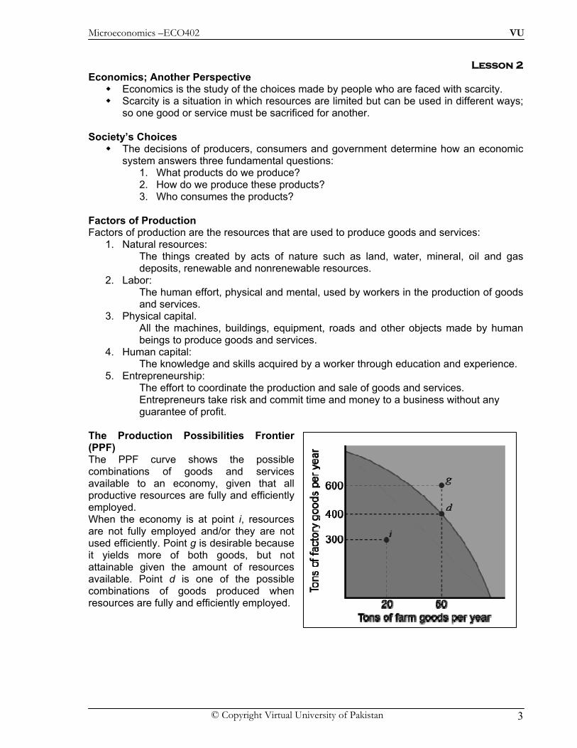
The Production Possibilities Frontier (PPF) The PPF curve shows the possible combinations of goods and services available to an economy, given that all productive resources are fully and efficiently employed. When the economy is at point i, resources are not fully employed and/or they are not used efficiently. Point g is desirable because it yields more of both goods, but not attainable given the amount of resources available. Point d is one of the possible combinations of goods produced when resources are fully and efficiently employed.

Microeconomics –ECO402 VU
© Copyright Virtual University of Pakistan 4
Scarcity and the PPF To increase the amount of farm goods by 10 tons, we must sacrifice 100 tons of factory goods. The PPF curve is bowed out because resources are not perfectly adaptable to the production of the two goods. As we increase the production of one good, we sacrifice progressively more of the other. Shifting the PPF Curve To increase the production of one good without decreasing the production of the other, the PPF curve must shift outward. The PPF curve shifts outward as a result of an increase in the economy’s resources OR a technological innovation that increases the output obtained from a given amount of resources. From point d, an additional 200 tons of factory goods or 20 tons of farm goods are now possible (or any combination in between).
Microeconomics –ECO402 VU
© Copyright Virtual University of Pakistan 5
Lesson 3
REAL VERSUS NOMINAL PRICES
Nominal price is the absolute or current dollar price of a good or service when it is sold. Real price is the price relative to an aggregate measure of prices or constant dollar
price. The Consumer Price Index (CPI) is an aggregate measure. Real prices are
emphasized to permit the analysis of relative prices.
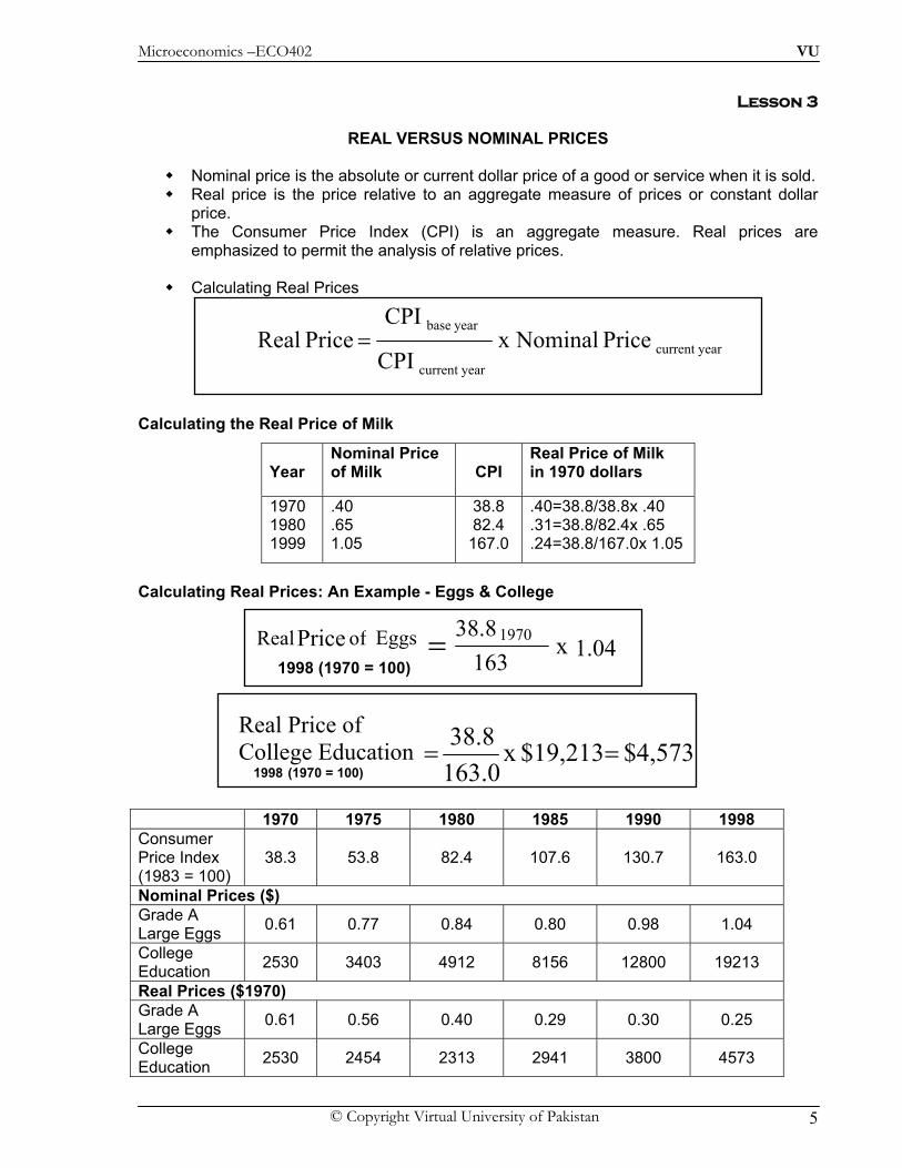
Calculating Real Prices
Calculating the Real Price of Milk
Calculating Real Prices: An Example - Eggs & College
1970 1975 1980 1985 1990 1998 Consumer Price Index (1983 = 100)
38.3 53.8 82.4 107.6 130.7 163.0
Nominal Prices ($) Grade A Large Eggs 0.61 0.77 0.84 0.80 0.98 1.04
College Education 2530 3403 4912 8156 12800 19213
Real Prices ($1970) Grade A Large Eggs 0.61 0.56 0.40 0.29 0.30 0.25
College Education 2530 2454 2313 2941 3800 4573
Year Nominal Price of Milk
CPI
Real Price of Milk in 1970 dollars
1970 1980 1999
.40
.65 1.05
38.8 82.4
167.0
.40=38.8/38.8x .40
.31=38.8/82.4x .65
.24=38.8/167.0x 1.05
yearcurrent yearcurrent
year basePrice Nominal x
CPI
CPI Price Real =
1.04x163
38.8Eggsof Price Real 1970=1998 (1970 = 100)
Real Price of College Education 1998 (1970 = 100)
$4,573$19,213x 163.038.8 ==
Microeconomics –ECO402 VU
© Copyright Virtual University of Pakistan 6
D
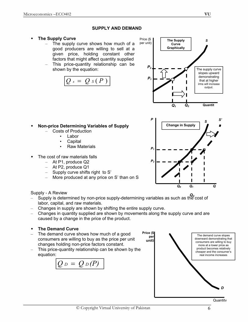
The demand curve slopes downward demonstrating that consumers are willing to buy
more at a lower price as product becomes relatively
cheaper and the consumer’s real income increases
Quantity
Price ($ per
unit)
SUPPLY AND DEMAND
The Supply Curve
– The supply curve shows how much of a good producers are willing to sell at a given price, holding constant other factors that might affect quantity supplied
– This price-quantity relationship can be shown by the equation:
Non-price Determining Variables of Supply – Costs of Production
• Labor • Capital • Raw Materials
The cost of raw materials falls
– At P1, produce Q2 – At P2, produce Q1 – Supply curve shifts right to S’ – More produced at any price on S’ than on S
Supply - A Review – Supply is determined by non-price supply-determining variables as such as the cost of
labor, capital, and raw materials. – Changes in supply are shown by shifting the entire supply curve. – Changes in quantity supplied are shown by movements along the supply curve and are
caused by a change in the price of the product.
The Demand Curve – The demand curve shows how much of a good
consumers are willing to buy as the price per unit changes holding non-price factors constant.
– This price-quantity relationship can be shown by the equation:
P S Change in Supply
Q
P1
P2
Q1 Q0
S’
)( PQQ Ss =
Q2
S
The supply curve slopes upward demonstrating that at higher
irms will increase output.
The Supply Curve
Graphically
Quantit
Price ($ per unit)
P1
P2
Q2 Q1
(P)QQ DD =

Microeconomics –ECO402 VU
© Copyright Virtual University of Pakistan 7
Non-price Determining Variables of Demand
– Income – Consumer Tastes – Price of Related Goods
• Substitutes • Complements
Income Increases – At P1, produce Q2 – At P2, produce Q1 – Demand Curve shifts right – More purchased at any price on D’
than on D
Demand - A Review – Demand is determined by non-price demand-determining variables, such as,
income, price of related goods, and tastes. – Changes in demand are shown by shifting the entire demand curve. – Changes in quantity demanded are shown by movements along the demand
curve.
The Market Mechanism Characteristics of the equilibrium or market
clearing price: – QD = QS – No shortage – No excess supply – No pressure on the price to change
The market price is above equilibrium – There is excess supply – Producers lower prices – Quantity demanded increases and
quantity supplied decreases – The market continues to adjust until
the equilibrium price is reached.
Quantity
D
S
The curves intersect at equilibrium, or market clearing, price. At P0 the
quantity supplied is equal to the quantity
demanded at Q0 .
P0
Price($ per
unit)
Q0
D P
QQ1
P2
Q0
P1
D’
Q2
Change in Demand
Quantity
D
S
P2
Q3
Assume the price is P1,then: 1) Qs : Q1 > Qd : Q2 2) Excess supply is Q1:Q2. 3) Producers lower price. 4) Quantity supplied decreases and quantity demanded increases. 5) Equilibrium at P2Q3
P1
Surplus
Price($ per unit) A Surplus
Q1 Q2

Microeconomics –ECO402 VU
© Copyright Virtual University of Pakistan 8
The market price is below equilibrium:
– There is a shortage – Producers raise prices – Quantity demanded decreases and
quantity supplied increases – The market continues to adjust until the
new equilibrium price is reached.
Market Mechanism Summary 1) Supply and demand interacts to determine the market-clearing price. 2) When not in equilibrium, the market will adjust to alleviate a shortage or surplus and return the market to equilibrium. 3) Markets must be competitive for the mechanism to be efficient.
D
S
Q1 Q2
P2
Shortage
Quantity
Price($ per unit)
Assume the price is P2,: 1) Qd : Q2 > Qs : Q1 2) Shortage is Q1:Q2. 3) Producers raise price. 4) Quantity supplied increases and quantity demanded decreases. 5) Equilibrium at P3, Q3
Q3
P3
Shortage

Microeconomics –ECO402 VU
© Copyright Virtual University of Pakistan 9
Lesson 4
Changes in Market Equilibrium
Equilibrium prices are determined by the relative level of supply and demand. Supply and demand are determined by particular values of supply and demand
determining variables. Changes in any one or combination of these variables can cause a change in the
equilibrium price and/or quantity.
Raw material prices fall – S shifts to S’ – Surplus @ P1 of Q1, Q2 – Equilibrium @ P3, Q3
Raw material prices Rise – S shifts to S’ – Shortage @ P1 of Q1, Q2 – Equilibrium @ P3, Q3
Income Increases – Demand shifts to D’ Shortage @ P1 of
Q1, Q2 – Equilibrium @ P3, Q3
S’
Q2
P
Q
S D
P3
Q3 Q1
P1
S’ S
Q2
P
Q
D
Q3
P3
P1
Q1
D’ S D
Q3
P3
Q2
P
Q Q1
P1

Microeconomics –ECO402 VU
© Copyright Virtual University of Pakistan 10
Income Decreases
– Demand shifts to D’ – Surplus @ P1 of Q1, Q2 – Equilibrium @ P3, Q3
Income Increases & raw material prices fall – The increase in D is greater than the increase
in S – Equilibrium price and quantity increase to P2,
Q2
Income Increases & raw material prices fall
– The increase in D is less than the increase in S
– Equilibrium price decrease to P2and quantity increase to Q2
Income Decreases & raw material prices Fall – The decrease in D is greater than the
increase in S – Equilibrium price and quantity decrease to P2
Q2
D S D’
Q1
P1
Q2
P
Q Q3
P3
D’ S’ P
Q
S
P2
Q2
D
P1
Q1
D’ S’
P
Q
S
P2
Q2
D
P1
Q1
D S’ P
Q
S
P2
Q2
D’
P1
Q1
Microeconomics –ECO402 VU
© Copyright Virtual University of Pakistan 11
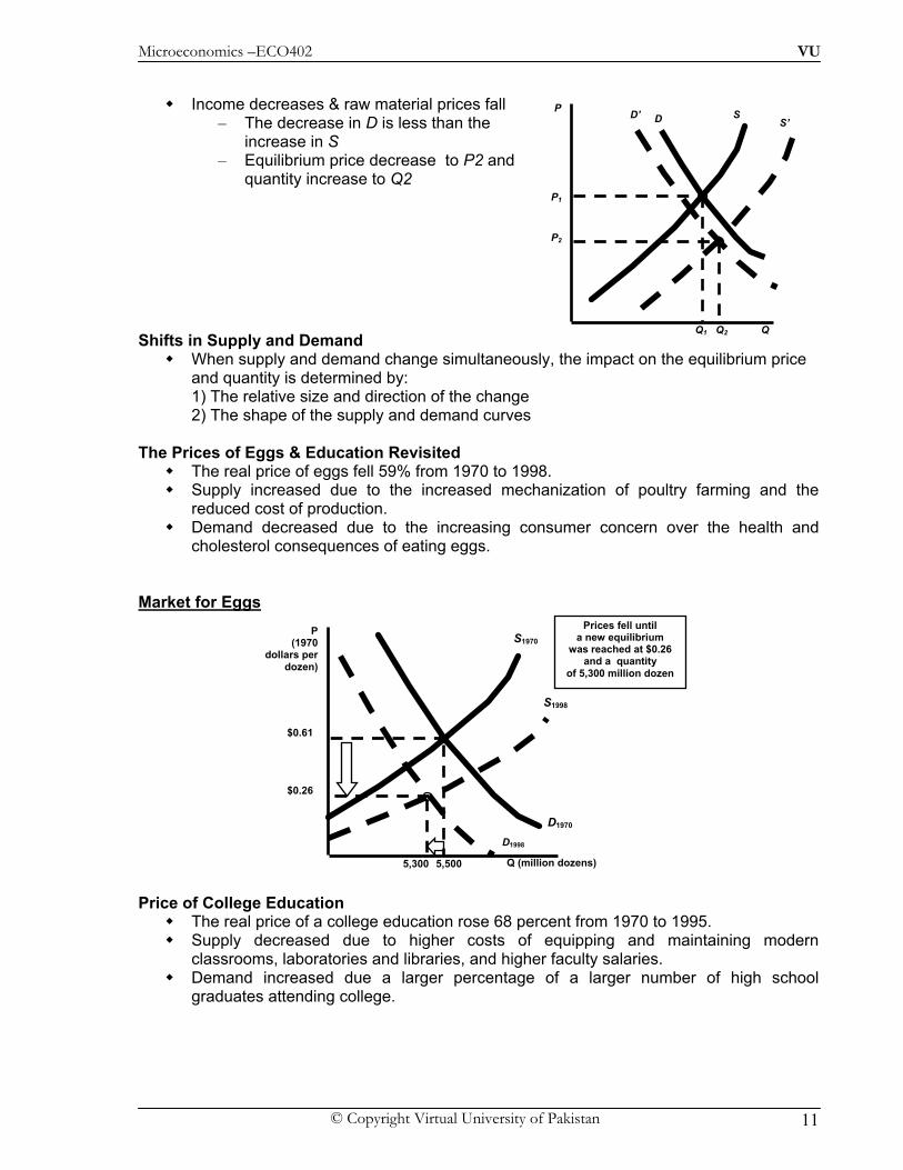
Income decreases & raw material prices fall
– The decrease in D is less than the increase in S
– Equilibrium price decrease to P2 and quantity increase to Q2
Shifts in Supply and Demand
When supply and demand change simultaneously, the impact on the equilibrium price and quantity is determined by:
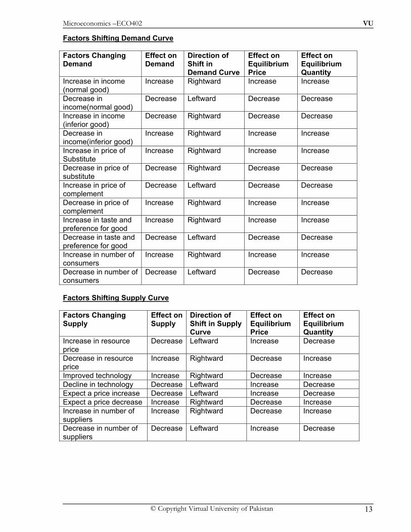
1) The relative size and direction of the change 2) The shape of the supply and demand curves The Prices of Eggs & Education Revisited
The real price of eggs fell 59% from 1970 to 1998. Supply increased due to the increased mechanization of poultry farming and the
reduced cost of production. Demand decreased due to the increasing consumer concern over the health and
cholesterol consequences of eating eggs. Market for Eggs Price of College Education
The real price of a college education rose 68 percent from 1970 to 1995. Supply decreased due to higher costs of equipping and maintaining modern
classrooms, laboratories and libraries, and higher faculty salaries. Demand increased due a larger percentage of a larger number of high school
graduates attending college.
D S’ P
Q
S
P2
Q2
D’
P1
Q1
Q (million dozens)
P (1970
dollars per dozen)
D1970
S1970
$0.61
5,500
D1998
S1998
Prices fell until a new equilibrium
was reached at $0.26 and a quantity
of 5,300 million dozen
$0.26
5,300

Microeconomics –ECO402 VU
© Copyright Virtual University of Pakistan 12
Market for College Education The Long-Run Behavior of Natural Resource Prices
Observations – Consumption of copper has increased about a hundred fold from 1880 through
1998 indicating a large increase in demand. – The real price for copper has remained relatively constant.
Changes in Market Equilibrium
Conclusion – Decreases in the costs of production have increased the supply by more than
enough to offset the increase in demand.
S1998
D1998 D1900
S1900 S1950
D1950
Long-Run Path of Price and
Price
Quantity
Q (millions of students enrolled)
P (annual cost
in 1970 dollars)
D1970
S1970
S1995
D1995
$4,573
12.3
Prices rose until a new equilibrium
was reached at $4,573 and a quantity
of 12.3 million students
$2,530
8.6
Microeconomics –ECO402 VU
© Copyright Virtual University of Pakistan 13
Factors Shifting Demand Curve Factors Changing Demand
Effect on Demand
Direction of Shift in Demand Curve
Effect on Equilibrium Price
Effect on Equilibrium Quantity
Increase in income (normal good)
Increase Rightward Increase Increase
Decrease in income(normal good)
Decrease Leftward Decrease Decrease
Increase in income (inferior good)
Decrease Rightward Decrease Decrease
Decrease in income(inferior good)
Increase Rightward Increase Increase
Increase in price of Substitute
Increase Rightward Increase Increase
Decrease in price of substitute
Decrease Rightward Decrease Decrease
Increase in price of complement
Decrease Leftward Decrease Decrease
Decrease in price of complement
Increase Rightward Increase Increase
Increase in taste and preference for good
Increase Rightward Increase Increase
Decrease in taste and preference for good
Decrease Leftward Decrease Decrease
Increase in number of consumers
Increase Rightward Increase Increase
Decrease in number of consumers
Decrease Leftward Decrease Decrease
Factors Shifting Supply Curve Factors Changing Supply
Effect on Supply
Direction of Shift in Supply Curve
Effect on Equilibrium Price
Effect on Equilibrium Quantity
Increase in resource price
Decrease Leftward Increase Decrease
Decrease in resource price
Increase Rightward Decrease Increase
Improved technology Increase Rightward Decrease Increase Decline in technology Decrease Leftward Increase Decrease Expect a price increase Decrease Leftward Increase Decrease Expect a price decrease Increase Rightward Decrease Increase Increase in number of suppliers
Increase Rightward Decrease Increase
Decrease in number of suppliers
Decrease Leftward Increase Decrease
Microeconomics –ECO402 VU
© Copyright Virtual University of Pakistan 14
ELASTICITIES OF SUPPLY AND DEMAND
Generally, elasticity is a measure of the sensitivity of one variable to another. It tells us the percentage change in one variable in response to a one percent change
in another variable. Price Elasticity of Demand
Measures the sensitivity of quantity demanded to price changes. It measures the percentage change in the quantity demanded for a good or
services that results from a one percent change in the price of that good or service.
The price elasticity of demand is:
Percentage change in Quantity Demanded Percentage change in Price
– The percentage change in a variable is the absolute change in the variable divided by the original level of the variable.
– So the price elasticity of demand is also:
PQ /Q P Q
E P /P Q P
Δ Δ= =
Δ Δ
Interpreting Price Elasticity of Demand Values 1) Because of the inverse relationship between P and Q; EP is negative. 2) If IEPI > 1, the percent change in quantity is greater than the percent change in price. We say the demand is price elastic.
3) If IEPI < 1, the percent change in quantity is less than the percent change in price. We say the demand is price inelastic.
The primary determinant of price elasticity of demand is the availability of substitutes. – Many substitutes demand is price elastic – Few substitutes demand is price inelastic –
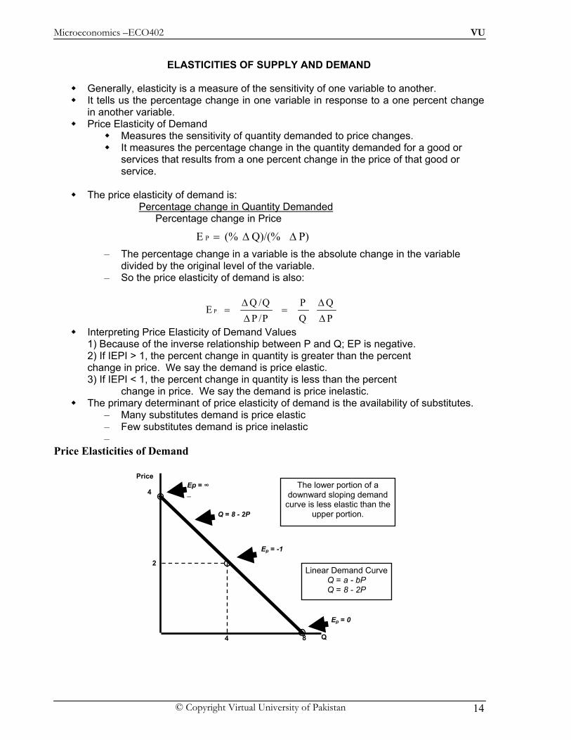
Price Elasticities of Demand
P)Q)/(%(% E P ΔΔ=
Q
Price
Q = 8 - 2P
Ep = -1
Ep = 0
The lower portion of a downward sloping demand
curve is less elastic than the upper portion.
4
8
Ep = ∞ _
2
4
Linear Demand CurveQ = a - bP Q = 8 - 2P
Microeconomics –ECO402 VU
© Copyright Virtual University of Pakistan 15
Q
Price
2 3 6 100
3
6
9
12
D
A
B
C
D
Ep = -1
Ep = -0.4
Ep = -3
Quantity
Price
Q*
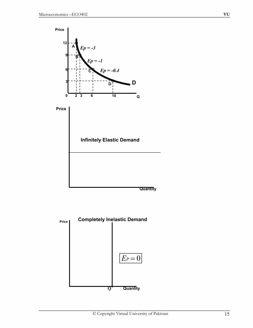
0 EP =
Quantity
Price Completely Inelastic Demand
Infinitely Elastic Demand
Microeconomics –ECO402 VU
© Copyright Virtual University of Pakistan 16
LESSON 5
Elasticities of supply and demand
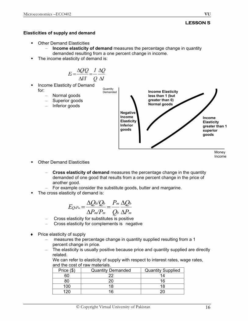
Other Demand Elasticities – Income elasticity of demand measures the percentage change in quantity
demanded resulting from a one percent change in income. The income elasticity of demand is:
IQ/Q I Q
E I/I Q I
Δ Δ= =Δ Δ
Income Elasticity of Demand for:
– Normal goods – Superior goods – Inferior goods
Other Demand Elasticities
– Cross elasticity of demand measures the percentage change in the quantity demanded of one good that results from a one percent change in the price of another good.
– For example consider the substitute goods, butter and margarine. The cross elasticity of demand is:
– Cross elasticity for substitutes is positive – Cross elasticity for complements is negative
♦ Price elasticity of supply
– measures the percentage change in quantity supplied resulting from a 1 percent change in price.
– The elasticity is usually positive because price and quantity supplied are directly related. We can refer to elasticity of supply with respect to interest rates, wage rates, and the cost of raw materials.
Price ($) Quantity Demanded Quantity Supplied 60 22 14 80 20 16
100 18 18 120 16 20
m
b
b
m
mm
bbPQ
PQ
QP
/PP/QQ E mb
ΔΔ
=ΔΔ
=
Negative Income Elasticity Inferior goods
Income Elasticity less than 1 (but greater than 0) Normal goods
Income Elasticity greater than 1 superior goods
Quantity Demanded
Money Income

Microeconomics –ECO402 VU
© Copyright Virtual University of Pakistan 17
Recall
PQ/Q P Q
E P/P Q P
Δ Δ= =
Δ Δ
Elasticity of demand when price is $80 is
Ep = 80/20 x -2/20 = -0.40 Elasticity of demand when price is $100 is
Ep = 100/18 x -2/20 = -0.56 Elasticity of supply when price is $80 is
Ep = 80/16 x 2/20 = 0.50 Elasticity of supply when price is $100 is
Ep = 100/18 x 2/20 = 0.56
The Market for Wheat – 1981 Supply Curve for Wheat
– QS = 1,800 + 240P – 1981 Demand Curve for Wheat
– QD = 3,550 - 266P – Equilibrium: Q S = Q D
1,800 240 3,550 266P P+ = −
506 1,750P = 3.46 /P bushel= 1,800 (240)(3.46) 2, 630 million bushelsQ = + =
3.46( 2.66) .035 Inelastic
2, 630D DP
QPE
Q PΔ
= = − = −Δ
3.46(2.40) .032 Inelastic
2,630S SP
QPE
Q PΔ
= = =Δ
– Assume the price of wheat is $4.00/bushel
3,550 (266)(4.00) 2, 486DQ = − =
4.00( 266) 0.43
2, 486DPQ = − = −
Supply (Qs) Demand (Qd) Equilibrium Price Qs = Qd
1981 1800 + 240P 3550 – 266P 1800 + 240P = 3550 – 266P 506P = 1750 P1981 = $3.46 / bushel
1998 1944 + 207P 3244 – 283P 1944 +207P = 3244 – 283P P1998 = $2.65 / bushel
Short-Run Versus Long-Run Elasticities
Price elasticity of demand varies with the amount of time consumers have to respond to a price.
Most goods and services: Short-run elasticity is less than long-run elasticity. (e.g. gasoline, Drs.)
Other Goods (durables): Short-run elasticity is greater than long-run elasticity (e.g. automobiles)

Microeconomics –ECO402 VU
© Copyright Virtual University of Pakistan 18
Gasoline: Short-Run and Long-Run Demand Curves Automobiles: Short-Run and Long-Run Demand Curves
Income elasticity also varies with the amount of time consumers have to respond to an income change.
Most goods and services: Income elasticity is greater in the long-run than in the short run.
Higher incomes may be converted into bigger cars so the income elasticity of demand for gasoline increases with time.
Other Goods (durables): Income elasticity is less in the long-run than in the short-run.
Originally, consumers will want to hold more cars. Later, purchases will only to be to replace old cars.
Gasoline and Automobiles are complementary goods. Gasoline
The long-run price and income elasticities are larger than the short-run elasticities.
Automobiles The long-run price and income elasticities are smaller than the short-run
elasticities.
DSR
DLR
People may put off immediate consumption, but eventually older cars
must be replaced.
Automobiles
Quantity
Price
DSR
DLR
People tend to drive smaller and more fuel efficient
cars in the long-run
Gasoline
Quantity
Price
Microeconomics –ECO402 VU
© Copyright Virtual University of Pakistan 19
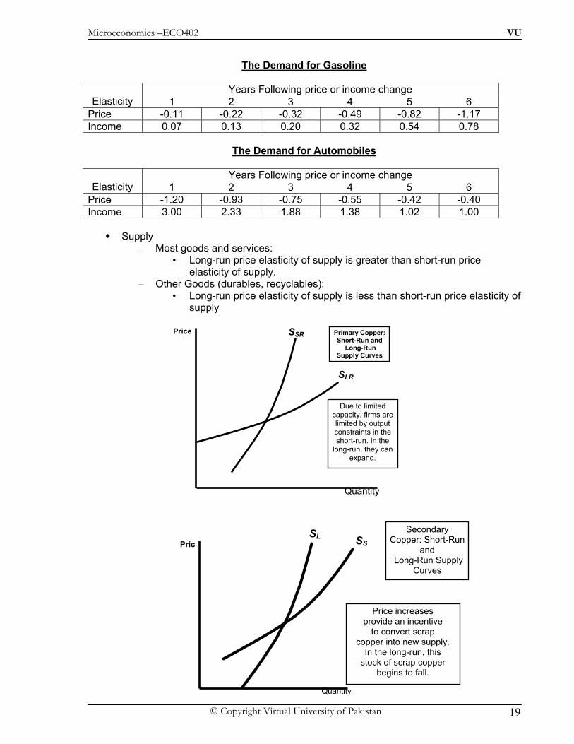
The Demand for Gasoline
Years Following price or income change
Elasticity 1 2 3 4 5 6 Price -0.11 -0.22 -0.32 -0.49 -0.82 -1.17 Income 0.07 0.13 0.20 0.32 0.54 0.78
The Demand for Automobiles
Years Following price or income change Elasticity 1 2 3 4 5 6
Price -1.20 -0.93 -0.75 -0.55 -0.42 -0.40 Income 3.00 2.33 1.88 1.38 1.02 1.00
Supply
– Most goods and services: • Long-run price elasticity of supply is greater than short-run price
elasticity of supply. – Other Goods (durables, recyclables):
• Long-run price elasticity of supply is less than short-run price elasticity of supply
SSR Primary Copper: Short-Run and
Long-Run Supply Curves
Quantity
Price
SLR
Due to limited capacity, firms are limited by output constraints in the short-run. In the
long-run, they can expand.
SS
Secondary Copper: Short-Run
and Long-Run Supply
Curves
Quantity
PricSL
Price increases provide an incentive
to convert scrap copper into new supply.
In the long-run, this stock of scrap copper
begins to fall.

Microeconomics –ECO402 VU
© Copyright Virtual University of Pakistan 20
Supply of Copper Price Elasticity of: Short Run Long run Primary Supply 0.20 1.60 Secondary Supply 0.43 0.31 Total Supply 0.25 1.50
Weather in Brazil and the price of Coffee in New York
Elasticity explains why coffee prices are very volatile. – Due to the differences in supply elasticity in the long-run and short run.
D
S
P0
Q0 Quantity
Price
P1
Short-Run 1) Supply is completely inelastic 2) Demand is relatively inelastic 3) Very large change in price
A freeze or drought decreases the
supply
S’
Q1
Coffee
Microeconomics –ECO402 VU
© Copyright Virtual University of Pakistan 21
D
S P0
Q0
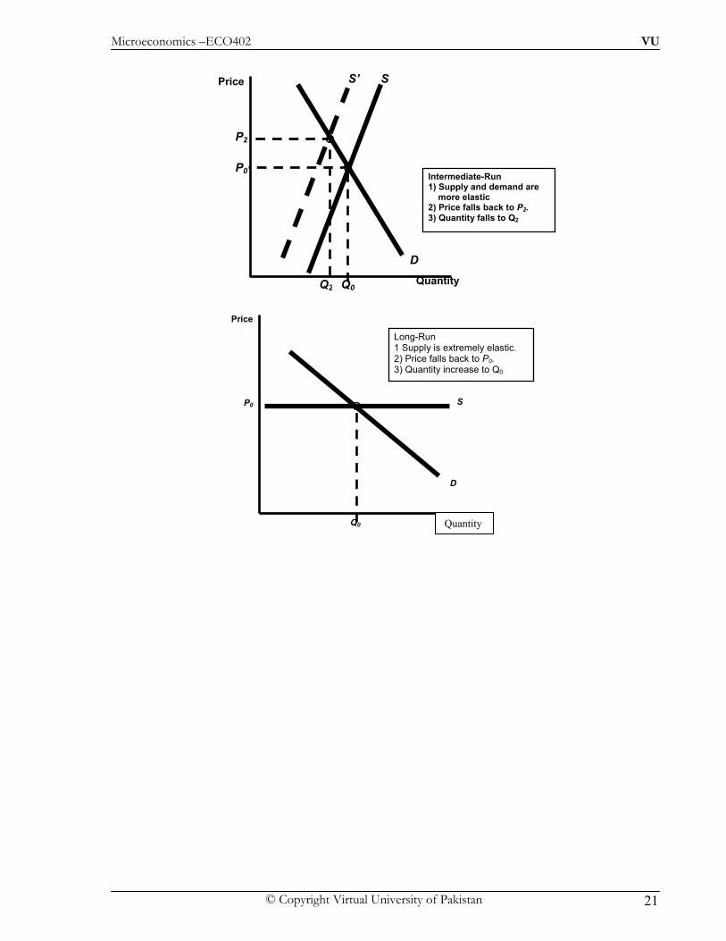
Long-Run 1 Supply is extremely elastic. 2) Price falls back to P0. 3) Quantity increase to Q0.
Price
Quantity
S’
D
S
P0
Q0
P2
Q2
Intermediate-Run1) Supply and demand are more elastic 2) Price falls back to P2. 3) Quantity falls to Q2
Quantity
Price

Microeconomics –ECO402 VU
© Copyright Virtual University of Pakistan 22
Lesson 6
Consumer Behavior
The explanation of how consumers allocate their resources (income) to the purchase of different goods and services to maximize their well being.
There are three steps involved in the study of consumer behavior. 1) We will study consumer preferences.
• To describe how and why people prefer one good to another. 2) Then we will turn to budget constraints.
• People have limited incomes. 3) Finally, we will combine consumer preferences and budget constraints
to determine consumer choices. • What combination of goods will consumers buy to maximize their
satisfaction? Consumer Preferences • Market Baskets
• A market basket is a collection of one or more commodities. • One market basket may be preferred over another market basket containing a
different combination of goods. • Three Basic Assumptions
1) Preferences are complete. 2) Preferences are transitive. 3) Consumers always prefer more of any good to less.
Market Basket Units of Food Units of Clothing A 20 30 B 10 50 D 40 20 E 30 40 G 10 20 H 10 40
Indifference curves represent all combinations of market baskets that provide the
same level of satisfaction to a person.
The consumer prefers A to all combinations in the blue box, while all those in the yellow box are preferred to A.
Food (units per week)
10
20
30
40
10 20 30 40
Clothing (units per week)
50
G
A
EH
B
D

Microeconomics –ECO402 VU
© Copyright Virtual University of Pakistan 23
Indifference Curves – Indifference curves slope downward to the right.
• If it sloped upward it would violate the assumption that more of any commodity is preferred to less.
– Any market basket lying above and to the right of an indifference curve is preferred to any market basket that lies on the indifference curve.
An indifference map is a set of indifference curves that describes a person’s
preferences for all combinations of two commodities. – Each indifference curve in the map shows the market baskets among which the
person is indifferent.
U1
Combination B,A, & D yield the same satisfaction
•E is preferred to U1
•U1 is preferred to H & G
Food(units per week)
10
20
30
40
10 20 30 40
Clothing (units per
week) 50
GD
A
EH
B
U2
U3
Food (units per week)
Clothing (units per
week)
U1
AB
D
Market basket A is preferred to B. Market basket B is preferred to D.

Microeconomics –ECO402 VU
© Copyright Virtual University of Pakistan 24
Indifference Curves – Finally, indifference curves cannot cross.
• This would violate the assumption that more is preferred to less.
The marginal rate of substitution (MRS) quantifies the amount of one good a consumer will give up to obtain more of another good.
– It is measured by the slope of the indifference curve.
UU
Food (units per week)
Clothing (units per week)
A
D
B
The consumer should be indifferent between A, B and D. However, B contains more of both goods than D.
Indifference Curves Cannot Cross
A
B
D
EG-1
-6
1
1
-4
-21
1
Observation: The amount of clothing given up for a unit of food decreases from 6 to 1
Food (units per week)
Clothing (units
per week)
2 3 4 51
2
4
6
8
10
12
14
16
Food (units per week)
Clothing (units
per week)
2 3 4 51
2
4
6
8
10
12
14
16 A
B
D
EG
-6
1
1
11
-4
-2-1
MRS = 6
MRS = 2
FCMRS Δ
Δ−=

Microeconomics –ECO402 VU
© Copyright Virtual University of Pakistan 25
We will now add a fourth assumption regarding consumer preference:
– Along an indifference curve there is a diminishing marginal rate of substitution. • Note the MRS for AB was 6, while that for DE was 2.
Marginal Rate of Substitution – Indifference curves are convex because as more of one good is consumed, a
consumer would prefer to give up fewer units of a second good to get additional units of the first one.
– Consumers prefer a balanced market basket – Perfect Substitutes and Perfect Complements
• Two goods are perfect substitutes when the marginal rate of substitution of one good for the other is constant.
• Two goods are complements when the indifference curves for the goods are shaped as right angles.
BADS – Things for which less is preferred to more
Example – Air pollution
Designing New Automobiles – Automobile executives must regularly decide when to introduce new models
and how much money to invest in restyling. – An analysis of consumer preferences would help to determine when and if car
companies should change the styling of their cars.
Orange Juice (glasses)
Apple Juice
(glasses)
2 3 41
1
2
3
4
0
PerfectSubstitutes
Right Shoes
Left Shoes
2 3 41
1
2
3
4
0
Perfect Complements

Microeconomics –ECO402 VU
© Copyright Virtual University of Pakistan 26
Designing New Automobiles – What Do You Think?
• How can we determine the consumers preference? Designing New Automobiles
– A recent study of automobile demand in the USA shows that over the past two decades most consumers have preferred styling over performance.
Growth of Japanese Imports – 1970’s and 1980’s
• 15% of domestic cars underwent a style change each year • This compares to 23% for imports
These consumers are willing to give up
considerable styling for additional
performance
Styling
Performance
Consumer Preference A:
High MRS
These consumers are willing to give up
considerable performance for additional styling
Styling
Performance
Consumer Preference B:
Low MRS
Microeconomics –ECO402 VU
© Copyright Virtual University of Pakistan 27
LESSON 7
CONSUMER PREFERENCES
Utility
– Numerical score representing the satisfaction that a consumer gets from a given market basket.
– If buying 3 copies of Microeconomics makes you happier than buying one shirt, then we say that the books give you more utility than the shirt.
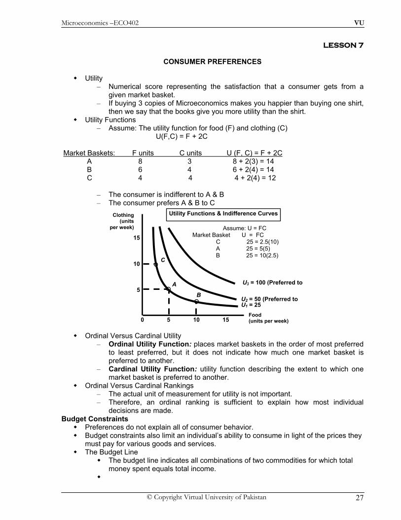
Utility Functions – Assume: The utility function for food (F) and clothing (C)
U(F,C) = F + 2C
Market Baskets: F units C units U (F, C) = F + 2C A 8 3 8 + 2(3) = 14 B 6 4 6 + 2(4) = 14 C 4 4 4 + 2(4) = 12
– The consumer is indifferent to A & B – The consumer prefers A & B to C
Ordinal Versus Cardinal Utility – Ordinal Utility Function: places market baskets in the order of most preferred
to least preferred, but it does not indicate how much one market basket is preferred to another.
– Cardinal Utility Function: utility function describing the extent to which one market basket is preferred to another.
Ordinal Versus Cardinal Rankings – The actual unit of measurement for utility is not important. – Therefore, an ordinal ranking is sufficient to explain how most individual
decisions are made. Budget Constraints
Preferences do not explain all of consumer behavior. Budget constraints also limit an individual’s ability to consume in light of the prices they
must pay for various goods and services. The Budget Line
The budget line indicates all combinations of two commodities for which total money spent equals total income.
Food (units per week) 10 155
5
10
15
0
Clothing (units
per week)
U1 = 25 U2 = 50 (Preferred to
U3 = 100 (Preferred to A
B
C
Assume: U = FC
Market Basket U = FC C 25 = 2.5(10) A 25 = 5(5) B 25 = 10(2.5)
Utility Functions & Indifference Curves

Microeconomics –ECO402 VU
© Copyright Virtual University of Pakistan 28
The Budget Line Let F equal the amount of food purchased, and C is the amount of clothing. Price of food = Pf and price of clothing = Pc Then Pf F is the amount of money spent on food, and Pc C is the amount of
money spent on clothing. The budget line then can be written:
Market Basket Food (F) Clothing (C) Total Spending Pf = ($1) Pc = ($2) PfF + PcC = I
A 0 40 $80 B 20 30 $80 D 40 20 $80 E 60 10 $80 G 80 0 $80
The Budget Line – As consumption moves along a budget line from the intercept, the consumer
spends less on one item and more on the other. – The slope of the line measures the relative cost of food and clothing. – The slope is the negative of the ratio of the prices of the two goods. – The slope indicates the rate at which the two goods can be substituted without
changing the amount of money spent. – The vertical intercept (I/PC), illustrates the maximum amount of C that can be
purchased with income I. – The horizontal intercept (I/PF), illustrates the maximum amount of F that can be
purchased with income I.
The Effects of Changes in Income and Prices – Income Changes
An increase in income causes the budget line to shift outward, parallel to the original line (holding prices constant).
A decrease in income causes the budget line to shift inward, parallel to the original line (holding prices constant).
ICPFP CF =+
Budget Line F + 2C = $80
CF/PPFC - 21- / Slope ==ΔΔ=1
2
(I/PC) = 40
40 60 80 = (I/PF) 20
10
20
30
0
A
B
D
E
G
Clothing (units
per week) Pc = $2 Pf = $1 I = $80
Food (units per week)

Microeconomics –ECO402 VU
© Copyright Virtual University of Pakistan 29
– Price Changes
• If the price of one good increases, the budget line shifts inward, pivoting from the other good’s intercept.
• If the price of one good decreases, the budget line shifts outward, pivoting from the other good’s intercept.
The Effects of Changes in Income and Prices – Price Changes
• If the two goods increase in price, but the ratio of the two prices is unchanged, the slope will not change.
• However, the budget line will shift inward to a point parallel to the original budget line.
• If the two goods decrease in price, but the ratio of the two prices is unchanged, the slope will not change.
• However, the budget line will shift outward to a point parallel to the original budget line.
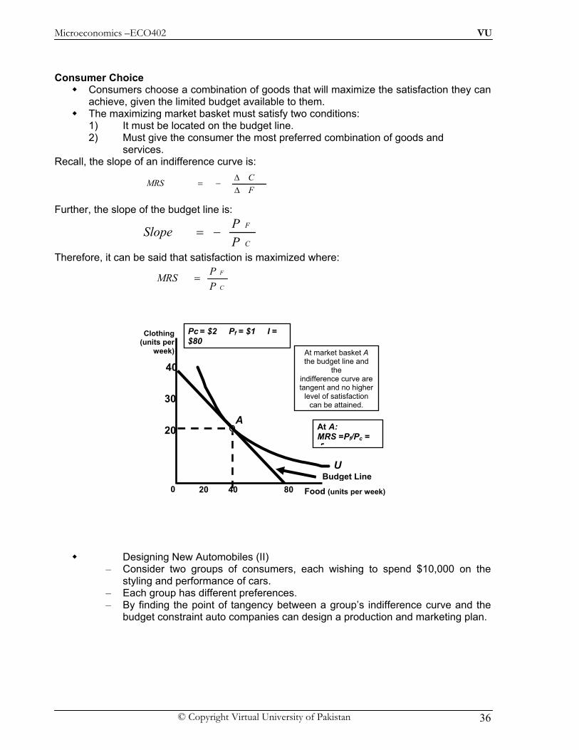
Consumer Choice Consumers choose a combination of goods that will maximize the satisfaction they can
achieve, given the limited budget available to them. The maximizing market basket must satisfy two conditions:
1) It must be located on the budget line.
Food (units per week)
Clothing(units
per week)
80 120 16040
20
40
60
80
0
A increase in income shifts
the budget line outward
(I = L2
(I = L1
L3
(I = $40
A decrease in income shifts
the budget line inward
Food (units per week)
Clothing (units
per week)
80 120 16040
40
(PF = 1)
L1
An increase in the price of food to $2.00 changes the slope of the budget line and rotates it inward.
L3
(PF = 2) (PF = 1/2)
L2
A decrease in the price of food to $.50 changes
the slope of the budget line and
rotates it outward.
Microeconomics –ECO402 VU
© Copyright Virtual University of Pakistan 30
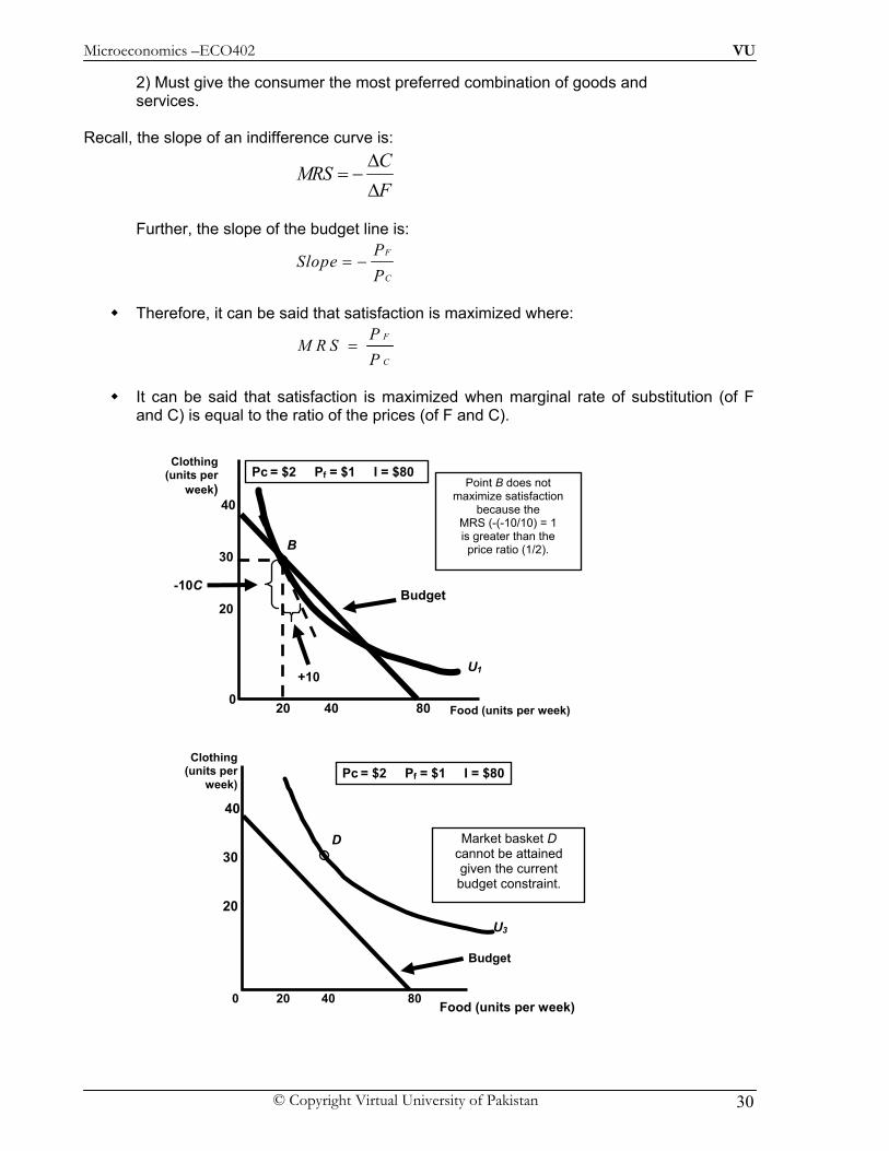
2) Must give the consumer the most preferred combination of goods and services. Recall, the slope of an indifference curve is:
CMRS
FΔ
= −Δ
Further, the slope of the budget line is:
F
C
PSlope
P= −
Therefore, it can be said that satisfaction is maximized where:
F
C
PM R S
P=
It can be said that satisfaction is maximized when marginal rate of substitution (of F
and C) is equal to the ratio of the prices (of F and C).
Food (units per week)
Clothing (units per
week)
40 8020
20
30
40
0
U1
B
Budget
Pc = $2 Pf = $1 I = $80Point B does not
maximize satisfaction because the
MRS (-(-10/10) = 1 is greater than the price ratio (1/2).
-10C
+10
Budget
U3
D Market basket D cannot be attained given the current budget constraint.
Pc = $2 Pf = $1 I = $80
Food (units per week)
Clothing (units per
week)
40 8020
20
30
40
0

Microeconomics –ECO402 VU
© Copyright Virtual University of Pakistan 31
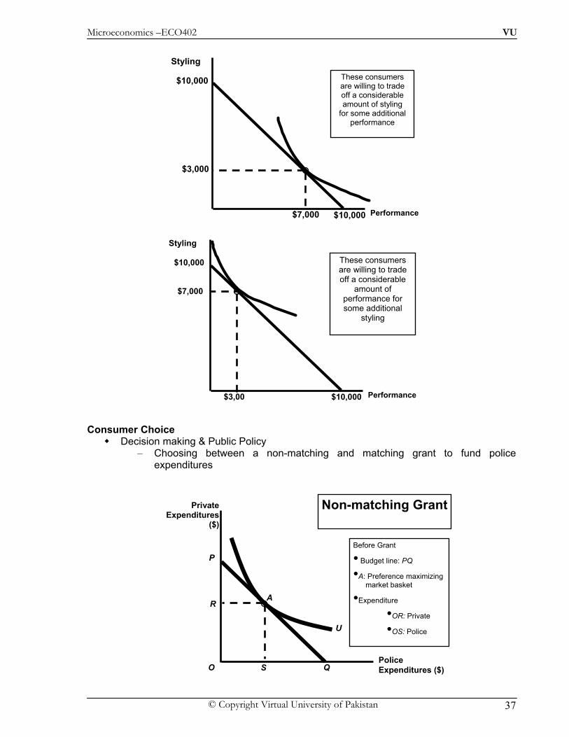
Designing New Automobiles (II)
– Consider two groups of consumers, each wishing to spend $10,000 on the styling and performance of cars.
– Each group has different preferences. – By finding the point of tangency between a group’s indifference curve and the – budget constraint auto companies can design a production and marketing plan.
U2
Pc = $2 Pf = $1 I = $80
Budget
A
At market basket A the budget line and the indifference curve are tangent and no higher
level of satisfaction can be attained.
At A: MRS =Pf/Pc = .5
Food (units per week)
Clothing (units per
week)
40 8020
20
30
40
0
Styling
Performance$10,000
$10,000
$3,000
These consumers are willing to trade off a considerable amount of styling
for some additional performance
$7,000
Styling
$10,000
$10,000
$3,000
These consumers are willing to trade off a considerable
amount of performance for some additional
styling
$7,000
Performance
Microeconomics –ECO402 VU
© Copyright Virtual University of Pakistan 32
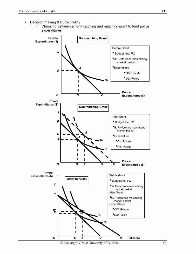
Decision making & Public Policy
– Choosing between a non-matching and matching grant to fund police expenditures
Non-matching Grant
PoliceExpenditures ($)
Private Expenditures ($)
O
P
Q
U1
A
Before Grant
• Budget line: PQ
•A: Preference maximizing market basket
•Expenditure
•OR: Private
•OS: Police
R
S
V
T
U3
U1
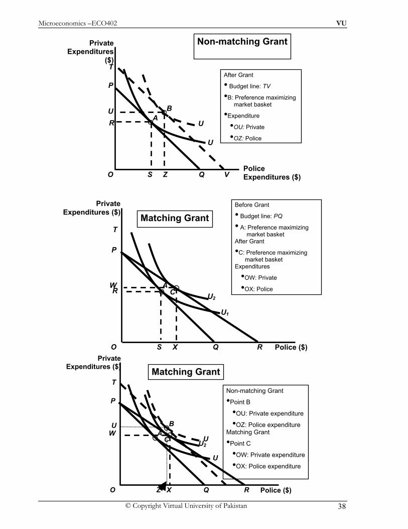
After Grant
• Budget line: TV
•B: Preference maximizing market basket
•Expenditure
•OU: Private
•OZ: Police
BU
Z
R
Non-matching Grant
P
PoliceExpenditures ($)
Private Expenditures ($)
O S Q
A
P
R
U2
T
U1
Matching Grant
Police ($)
Private Expenditures ($)
O QS
R
Before Grant
• Budget line: PQ
• A: Preference maximizing market basket After Grant
•C: Preference maximizing market basket Expenditures
•OW: Private
•OX: Police C
X
W
Microeconomics –ECO402 VU
© Copyright Virtual University of Pakistan 33
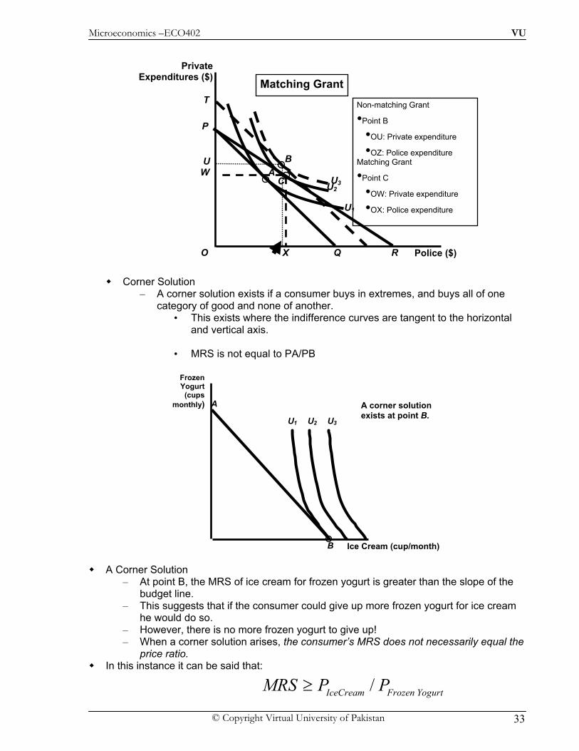
Corner Solution – A corner solution exists if a consumer buys in extremes, and buys all of one
category of good and none of another. • This exists where the indifference curves are tangent to the horizontal
and vertical axis. • MRS is not equal to PA/PB
A Corner Solution – At point B, the MRS of ice cream for frozen yogurt is greater than the slope of the
budget line. – This suggests that if the consumer could give up more frozen yogurt for ice cream
he would do so. – However, there is no more frozen yogurt to give up! – When a corner solution arises, the consumer’s MRS does not necessarily equal the
price ratio. In this instance it can be said that:
/IceCream Frozen YogurtMRS P P≥
T
U3
U1
Non-matching Grant
•Point B
•OU: Private expenditure
•OZ: Police expenditure Matching Grant
•Point C
•OW: Private expenditure
•OX: Police expenditure
W
X
Matching Grant
P
Police ($)
Private Expenditures ($)
O Q
AU2
C
R
BU
Ice Cream (cup/month)
Frozen Yogurt
(cups monthly)
B
A
U2 U3 U1
A corner solution exists at point B.

Microeconomics –ECO402 VU
© Copyright Virtual University of Pakistan 34
– If the MRS is, in fact, significantly greater than the price ratio, then a small decrease in the price of frozen yogurt will not alter the consumer’s market basket.
– A college Trust Fund – Suppose Jane Doe’s parents set up a trust fund for her college education. – Originally, the money must be used for education. – If part of the money could be used for the purchase of other goods, her
consumption preferences change.
The trust fund shifts the budget line
P
Q Education ($)
Other Consumption
($)
U
A College Trust Fund
A
U
A: Consumption before the trust fund
B
B: Requirement that the trust fund must be spent on education C
U C: If the trust could be spent on other goods
Microeconomics –ECO402 VU
© Copyright Virtual University of Pakistan 35
LESSON 8
Note it is repeated Consumer Preferences
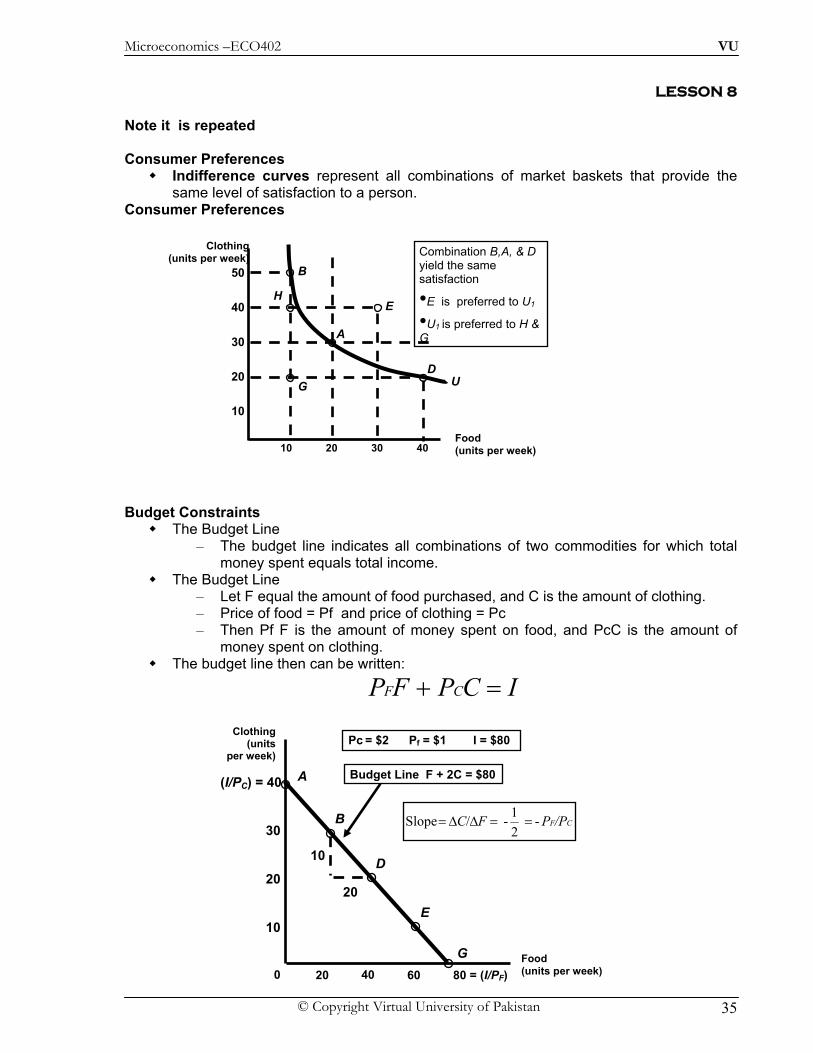
Indifference curves represent all combinations of market baskets that provide the same level of satisfaction to a person.
Consumer Preferences Budget Constraints
The Budget Line – The budget line indicates all combinations of two commodities for which total
money spent equals total income. The Budget Line
– Let F equal the amount of food purchased, and C is the amount of clothing. – Price of food = Pf and price of clothing = Pc – Then Pf F is the amount of money spent on food, and PcC is the amount of
money spent on clothing. The budget line then can be written:
F CP F P C I+ =
U
Combination B,A, & D yield the same satisfaction
•E is preferred to U1
•U1 is preferred to H & G
Food (units per week)
10
20
30
40
10 20 30 40
Clothing (units per week)
50
G D
A
EH
B
Budget Line F + 2C = $80
CF/PPFC - 21- / Slope ==ΔΔ=
10
20
(I/PC) = 40
Food (units per week) 40 60 80 = (I/PF)20
10
20
30
0
A
B
D
E
G
Clothing (units
per week) Pc = $2 Pf = $1 I = $80
Microeconomics –ECO402 VU
© Copyright Virtual University of Pakistan 36
Consumer Choice
Consumers choose a combination of goods that will maximize the satisfaction they can achieve, given the limited budget available to them.
The maximizing market basket must satisfy two conditions: 1) It must be located on the budget line. 2) Must give the consumer the most preferred combination of goods and services. Recall, the slope of an indifference curve is: Further, the slope of the budget line is: Therefore, it can be said that satisfaction is maximized where:
Designing New Automobiles (II) – Consider two groups of consumers, each wishing to spend $10,000 on the
styling and performance of cars. – Each group has different preferences. – By finding the point of tangency between a group’s indifference curve and the
budget constraint auto companies can design a production and marketing plan.
FCMRS
ΔΔ
−=
C
F
PPSlope −=
C
F
PPMRS =
U
Pc = $2 Pf = $1 I = $80
Budget Line
A
At market basket A the budget line and
the indifference curve are tangent and no higher
level of satisfaction can be attained.
At A:MRS =Pf/Pc = 5
Food (units per week)
Clothing(units per
week)
40 8020
20
30
40
0
Microeconomics –ECO402 VU
© Copyright Virtual University of Pakistan 37
Styling
Performance $10,000
$10,000
$3,000
These consumers are willing to trade off a considerable amount of styling
for some additional performance
$7,000
Consumer Choice
Decision making & Public Policy – Choosing between a non-matching and matching grant to fund police
expenditures
Styling
$10,000
$10,000
$3,00
These consumers are willing to trade off a considerable
amount of performance for some additional
styling
$7,000
Performance
Non-matching Grant
Police Expenditures ($)
Private Expenditures
($)
O
P
Q
U
A
Before Grant
• Budget line: PQ
•A: Preference maximizing market basket
•Expenditure
•OR: Private
•OS: Police
R
S
Microeconomics –ECO402 VU
© Copyright Virtual University of Pakistan 38
P
R
U2
T
U1
Matching Grant
Police ($)
Private Expenditures ($)
O QS
R
Before Grant
• Budget line: PQ
• A: Preference maximizing market basket After Grant
•C: Preference maximizing market basket Expenditures
•OW: Private
•OX: Police C
X
W A
T
U
U
Non-matching Grant
•Point B
•OU: Private expenditure
•OZ: Police expenditure Matching Grant
•Point C
•OW: Private expenditure
•OX: Police expenditure
W
X
Matching Grant
P
Police ($)
Private Expenditures ($)
O Q
A U2
C
R
BU
Z
V
T
U
U
After Grant
• Budget line: TV
•B: Preference maximizing market basket
•Expenditure
•OU: Private
•OZ: Police
BU
Z
R
Non-matching Grant
P
Police Expenditures ($)
Private Expenditures
($)
O S Q
A
Microeconomics –ECO402 VU
© Copyright Virtual University of Pakistan 39
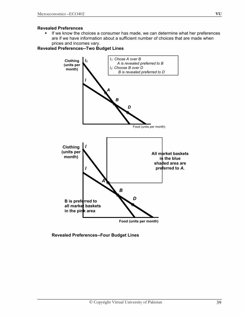
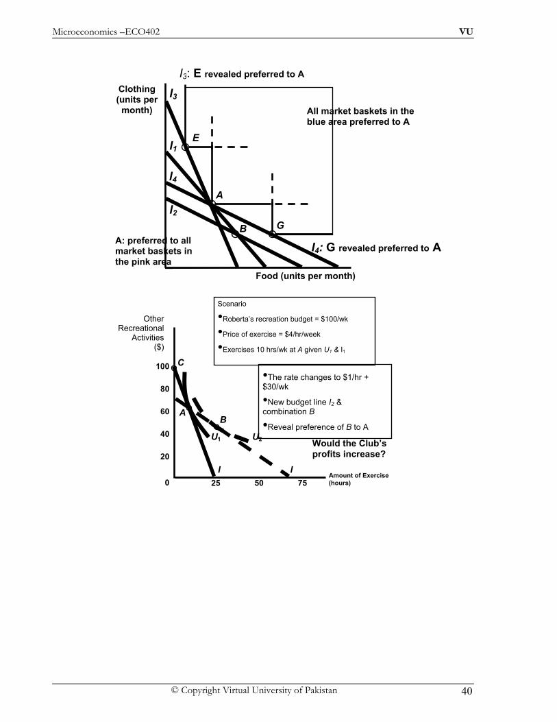
Revealed Preferences
If we know the choices a consumer has made, we can determine what her preferences are if we have information about a sufficient number of choices that are made when prices and incomes vary.
Revealed Preferences--Two Budget Lines Revealed Preferences--Four Budget Lines
D
l1
l
B
A
I1: Chose A over B A is revealed preferred to B l2: Choose B over D B is revealed preferred to D
Food (units per month)
Clothing (units per
month)
B is preferred to all market baskets in the pink area
l
B
l
D
A
All market baskets in the blue
shaded area are preferred to A.
Food (units per month)
Clothing (units per
month)
Microeconomics –ECO402 VU
© Copyright Virtual University of Pakistan 40
All market baskets in the blue area preferred to A
Food (units per month)
Clothing (units per
month)
l1
l2
l3
l4
A: preferred to all market baskets in the pink area
E
B
A
G
I3: E revealed preferred to A
I4: G revealed preferred to A
Amount of Exercise (hours)
Other Recreational
Activities ($)
0 25 50 75
20
40
60
80
100
l
C
l
U2
B
•The rate changes to $1/hr + $30/wk
•New budget line I2 & combination B
•Reveal preference of B to A U1
A
Scenario
•Roberta’s recreation budget = $100/wk
•Price of exercise = $4/hr/week
•Exercises 10 hrs/wk at A given U1 & I1
Would the Club’s profits increase?
Microeconomics –ECO402 VU
© Copyright Virtual University of Pakistan 41
Lesson 9
MARGINAL UTILITY AND CONSUMER CHOICE
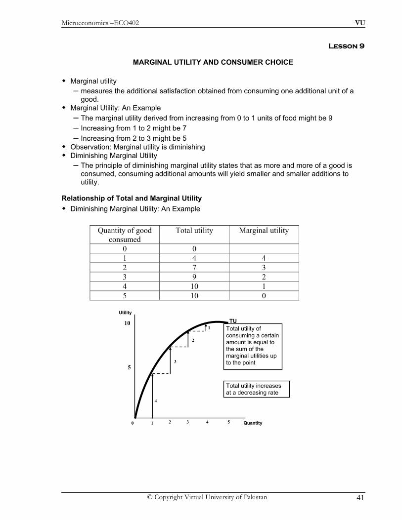
Marginal utility – measures the additional satisfaction obtained from consuming one additional unit of a
good. Marginal Utility: An Example
– The marginal utility derived from increasing from 0 to 1 units of food might be 9 – Increasing from 1 to 2 might be 7 – Increasing from 2 to 3 might be 5
Observation: Marginal utility is diminishing Diminishing Marginal Utility
– The principle of diminishing marginal utility states that as more and more of a good is consumed, consuming additional amounts will yield smaller and smaller additions to utility.
Relationship of Total and Marginal Utility Diminishing Marginal Utility: An Example
Quantity of good consumed
Total utility Marginal utility
0 0 1 4 4 2 7 3 3 9 2 4 10 1 5 10 0
5
10
0 5 4 3 2 1
Utility
Quantity
Total utility of consuming a certain amount is equal to the sum of the marginal utilities up to the point
Total utility increases at a decreasing rate
TU
4
3
2
1

Microeconomics –ECO402 VU
© Copyright Virtual University of Pakistan 42
Marginal Utility and Consumer Choice
Marginal Utility and the Indifference Curve – If consumption moves along an indifference curve, the additional utility derived from an
increase in the consumption of one good, food (F), must balance the loss of utility from the decrease in the consumption in the other good, clothing (C).
Formally:
Rearranging:
Because: ( )/ of F for CC F MRS− Δ Δ =
F CMRS MU /MU=
When consumers maximize satisfaction the: F CMRS P /P=
Since the MRS is also equal to the ratio of the marginal utilities of consuming F and C, it follows that:
F C F CMU/MU P /P=
Which gives the equation for utility maximization?
/ /F F C CMU P MU P=
Total utility is maximized when the budget is allocated so that the marginal utility per dollar of expenditure is the same for each good.
This is referred to as the equal marginal principle.
0 = MUF (ΔF) + MUC (ΔC)
- (ΔC/ ΔF) = MUF / MUC
5
0 5 4 3 2 1
Marginal Utility
Quantity
The fact that total utility increases at a decreasing rate is shown by negative slope of marginal utility curve
MU
3 2
1
4
Microeconomics –ECO402 VU
© Copyright Virtual University of Pakistan 43
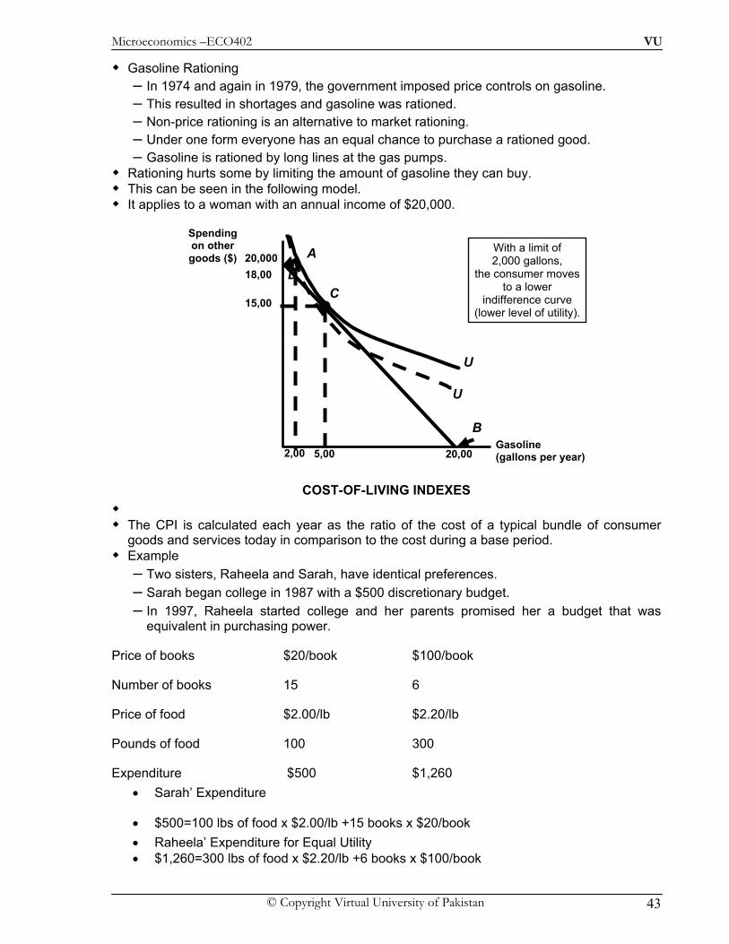
Gasoline Rationing – In 1974 and again in 1979, the government imposed price controls on gasoline. – This resulted in shortages and gasoline was rationed. – Non-price rationing is an alternative to market rationing. – Under one form everyone has an equal chance to purchase a rationed good. – Gasoline is rationed by long lines at the gas pumps.
Rationing hurts some by limiting the amount of gasoline they can buy. This can be seen in the following model. It applies to a woman with an annual income of $20,000.
COST-OF-LIVING INDEXES The CPI is calculated each year as the ratio of the cost of a typical bundle of consumer
goods and services today in comparison to the cost during a base period. Example
– Two sisters, Raheela and Sarah, have identical preferences. – Sarah began college in 1987 with a $500 discretionary budget. – In 1997, Raheela started college and her parents promised her a budget that was
equivalent in purchasing power.
Price of books $20/book $100/book
Number of books 15 6
Price of food $2.00/lb $2.20/lb
Pounds of food 100 300
Expenditure $500 $1,260 • Sarah’ Expenditure
• $500=100 lbs of food x $2.00/lb +15 books x $20/book • Raheela’ Expenditure for Equal Utility • $1,260=300 lbs of food x $2.20/lb +6 books x $100/book
B
20,00
A
Gasoline (gallons per year)
Spending on other goods ($) 20,000
5,00
U
C15,00
2,00
D
With a limit of 2,000 gallons,
the consumer moves to a lower
indifference curve (lower level of utility).
18,00
U
Microeconomics –ECO402 VU
© Copyright Virtual University of Pakistan 44
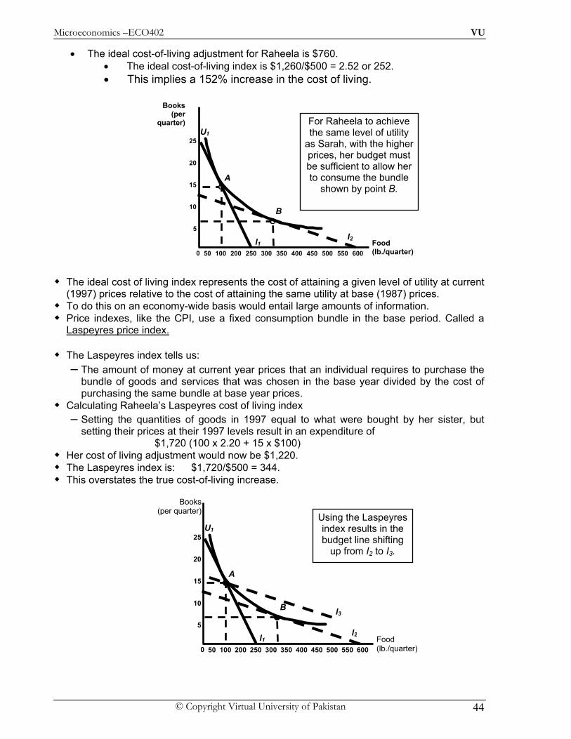
• The ideal cost-of-living adjustment for Raheela is $760. • The ideal cost-of-living index is $1,260/$500 = 2.52 or 252. • This implies a 152% increase in the cost of living.
The ideal cost of living index represents the cost of attaining a given level of utility at current (1997) prices relative to the cost of attaining the same utility at base (1987) prices.
To do this on an economy-wide basis would entail large amounts of information. Price indexes, like the CPI, use a fixed consumption bundle in the base period. Called a
Laspeyres price index.
The Laspeyres index tells us: – The amount of money at current year prices that an individual requires to purchase the
bundle of goods and services that was chosen in the base year divided by the cost of purchasing the same bundle at base year prices.
Calculating Raheela’s Laspeyres cost of living index – Setting the quantities of goods in 1997 equal to what were bought by her sister, but
setting their prices at their 1997 levels result in an expenditure of $1,720 (100 x 2.20 + 15 x $100)
Her cost of living adjustment would now be $1,220. The Laspeyres index is: $1,720/$500 = 344. This overstates the true cost-of-living increase.
For Raheela to achieve the same level of utility
as Sarah, with the higher prices, her budget must be sufficient to allow her to consume the bundle
shown by point B.
l2
B
l1
U1
A
Food (lb./quarter)
Books (per
quarter)
450
25
20
15
10
5
0 60050 100 200 250 300 350 400 550500
l2
Using the Laspeyres index results in the budget line shifting
up from I2 to I3.
l3 B
l1
U1
A
Food (lb./quarter)
Books (per quarter)
450
25
20
15
10
5
0 60050 100 200 250 300 350 400 550500

Microeconomics –ECO402 VU
© Copyright Virtual University of Pakistan 45
What Do You Think? – Does the Laspeyres index always overstate the true cost-of-living index?
Yes! – The Laspeyres index assumes that consumers do not alter their consumption patterns
as prices change. – By increasing purchases of those items that have become relatively cheaper, and
decreasing purchases of the relatively more expensive items consumers can achieve the same level of utility without having to consume the same bundle of goods.
The Paasche Index – Calculates the amount of money at current-year prices that an individual requires to
purchase a current bundle of goods and services divided by the cost of purchasing the same bundle in the base year.
Comparing the Two Indexes – Suppose: – Two goods: Food (F) and Clothing (C)
Comparing the Two Indexes – Let:
• PFt & PCt be current year prices
• PFb & PCb be base year prices
• Ft & Ct be current year quantities
• Fb & Cb be base year quantities – Both indexes involve ratios that involve today’s current year prices, PFt and PCt. – However, the Laspeyres index relies on base year consumption, Fb and Cb. – Whereas, the Paasche index relies on today’s current consumption, Ft and Ct .
Then a comparison of the Laspeyres and Paasche indexes gives the following equations:
– Sarah
(1990)
• Cost of base-year bundle at current prices equals $1,720 (100 lbs x $2.20/lb + 15 books x $100/book)
• Cost of same bundle at base year prices is $500 (100 lbs x $2.00/lb + 15 books x $20/book)
– Sarah (1990)
1 720344
500$ ,
LI$
= =
• Cost of buying current year bundle at current year prices is $1,260 (300 lbs x $2.20/lb + 6 books x $100/book)
PFt Fb + PCt Cb
PFb Fb + PCb Cb
PI = ------------------------ PFt Ft + PCt Ct PFb Ft + PCb Ct
LI = -----------------------

Microeconomics –ECO402 VU
© Copyright Virtual University of Pakistan 46
• Cost of the same bundle at base year prices is $720 (300 lbs x $2/lb + 6 books x $20/book)
1 260
175720
$ ,PI
$= =
The Paasche index will understate the cost of living because it assumes that the individual will buy the current year bundle in the base year.
Microeconomics –ECO402 VU
© Copyright Virtual University of Pakistan 47
Lesson 10
Review of Consumer Equilibrium Consumer Preferences Budget Constraint Consumer Choices
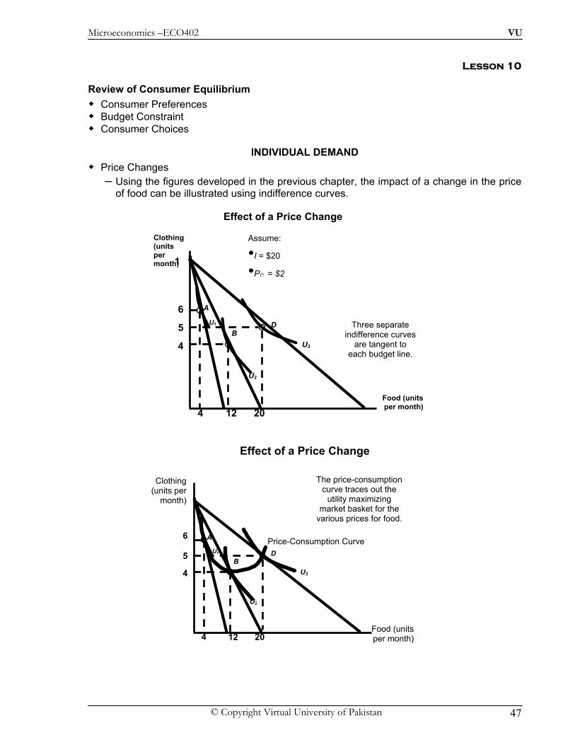
INDIVIDUAL DEMAND Price Changes
– Using the figures developed in the previous chapter, the impact of a change in the price of food can be illustrated using indifference curves.
Effect of a Price Change
Effect of a Price Change
Food (units per month)
Clothing (units per month)
Assume:
•I = $20
•PC = $21
4
5
6
U2
U3
A
BDU1
4 12 20
Three separate indifference curves
are tangent to each budget line.
Price-Consumption Curve
Food (units per month)
Clothing (units per
month)
4
5
6
U2
U3
A
BDU1
4 12 20
The price-consumption curve traces out the
utility maximizing market basket for the
various prices for food.
Microeconomics –ECO402 VU
© Copyright Virtual University of Pakistan 48
Effect of a Price Change
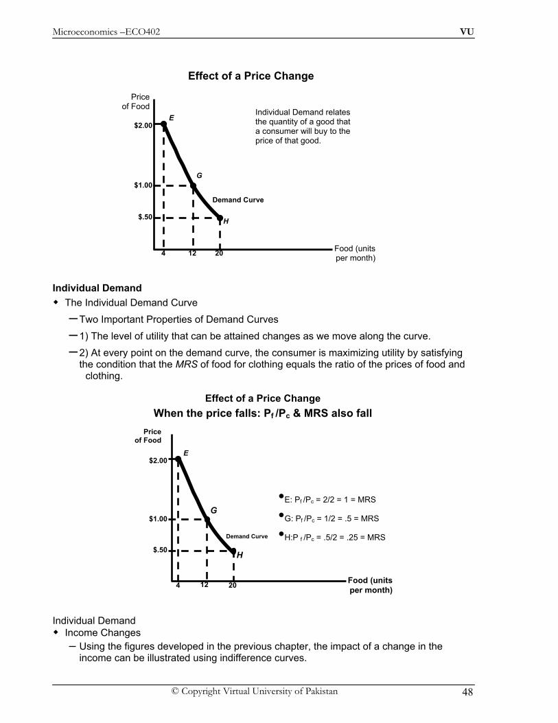
Individual Demand The Individual Demand Curve
– Two Important Properties of Demand Curves
– 1) The level of utility that can be attained changes as we move along the curve. – 2) At every point on the demand curve, the consumer is maximizing utility by satisfying
the condition that the MRS of food for clothing equals the ratio of the prices of food and clothing.
Effect of a Price Change When the price falls: Pf /Pc & MRS also fall
Individual Demand
Income Changes – Using the figures developed in the previous chapter, the impact of a change in the
income can be illustrated using indifference curves.
Demand Curve
Individual Demand relates the quantity of a good that a consumer will buy to the price of that good.
Food (units per month)
Price of Food
H
E
G
$2.00
4 12 20
$1.00
$.50
Demand Curve
•E: Pf /Pc = 2/2 = 1 = MRS
•G: Pf /Pc = 1/2 = .5 = MRS
•H:P f /Pc = .5/2 = .25 = MRS
Food (units per month)
Price of Food
H
E
G
$2.00
4 12 20
$1.00
$.50

Microeconomics –ECO402 VU
© Copyright Virtual University of Pakistan 49
Effects of Income Changes
Effects of Income Changes
– The income-consumption curve traces out the utility-maximizing combinations of food and clothing associated with every income level.
– An increase in income shifts the budget line to the right, increasing consumption along the income-consumption curve.
– Simultaneously, the increase in income shifts the demand curve to the right. Normal Good vs. Inferior Good
– Income Changes
• When the income-consumption curve has a positive slope:
–The quantity demanded increases with income.
–The income elasticity of demand is positive.
–The good is a normal good.
• When the income-consumption curve has a negative slope:
Food (units per month)
Clothing (units per
month)
An increase in income, with the prices fixed,
causes consumers to alter their choice of market basket.
Income-Consumption Curve
3
4
A U1
5
10
BU2
D7
16
U3
Assume: Pf = $1 Pc = $2 I = $10, $20, $30
Food (units per month)
Price of
food An increase in income, from $10 to $20 to $30, with the prices fixed, shifts the consumer’s demand curve to the right.
$100
4
D1
E
10
D2
G
16
D3
H

Microeconomics –ECO402 VU
© Copyright Virtual University of Pakistan 50
Tea (units per month)
Coffee(units per
month)
15
30
U3
C
Income-ConsumptionCurve
…but Tea becomes an inferior good when the income
consumption curve bends backward
between B and C.
105 20
5
10
A U1
B
U2
Both Tea and Coffee behave as a normal good, between A and B...
–The quantity demanded decreases with income.
–The income elasticity of demand is negative.
–The good is an inferior good.
An Inferior Good
Engel Curves Engel Curves
–Engel curves relate the quantity of good consumed to income. –If the good is a normal good, the Engel curve is upward sloping. –If the good is an inferior good, the Engel curve is downward sloping.
Food (unitsper month)
30
4 8 12
10
Income ($ per
month)
20
160
Engel curves slope
upward for normal goods.
Engel curves slope backward bending for inferior goods.
Inferior
Normal
Food (units per month)
30
4 8 12
10
Income($ per
month)
20
160
Microeconomics –ECO402 VU
© Copyright Virtual University of Pakistan 51
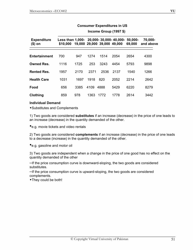
Consumer Expenditures in US
Entertainment 700 947 1274 1514 2054 2654 4300
Owned Res. 1116 1725 253 3243 4454 5793 9898
Rented Res. 1957 2170 2371 2536 2137 1540 1266
Health Care 1031 1697 1918 820 2052 2214 2642
Food 656 3385 4109 4888 5429 6220 8279
Clothing 859 978 1363 1772 1778 2614 3442
Individual Demand Substitutes and Complements
1) Two goods are considered substitutes if an increase (decrease) in the price of one leads to an increase (decrease) in the quantity demanded of the other.
•e.g. movie tickets and video rentals
2) Two goods are considered complements if an increase (decrease) in the price of one leads to a decrease (increase) in the quantity demanded of the other.
•e.g. gasoline and motor oil
3) Two goods are independent when a change in the price of one good has no effect on the quantity demanded of the other –If the price consumption curve is downward-sloping, the two goods are considered substitutes. –If the price consumption curve is upward-sloping, the two goods are considered complements.
They could be both!
Expenditure Less than 1,000- 20,000- 30,000- 40,000- 50,000- 70,000- ($) on $10,000 19,000 29,000 39,000 49,000 69,000 and above
Income Group (1997 $)
Microeconomics –ECO402 VU
© Copyright Virtual University of Pakistan 52
Lesson 11
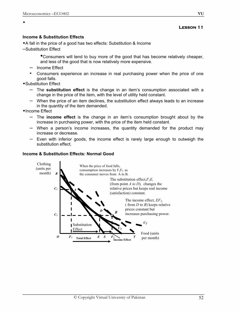
Income & Substitution Effects A fall in the price of a good has two effects: Substitution & Income
–Substitution Effect
•Consumers will tend to buy more of the good that has become relatively cheaper, and less of the good that is now relatively more expensive.
– Income Effect • Consumers experience an increase in real purchasing power when the price of one
good falls. Substitution Effect
– The substitution effect is the change in an item’s consumption associated with a change in the price of the item, with the level of utility held constant.
– When the price of an item declines, the substitution effect always leads to an increase in the quantity of the item demanded.
Income Effect – The income effect is the change in an item’s consumption brought about by the
increase in purchasing power, with the price of the item held constant. – When a person’s income increases, the quantity demanded for the product may
increase or decrease. – Even with inferior goods, the income effect is rarely large enough to outweigh the
substitution effect.
Income & Substitution Effects: Normal Good
Food (units per month)O
Clothing (units per
month) R
F1 S
C1 A
U1
The income effect, EF2, ( from D to B) keeps relative prices constant but increases purchasing power.
Income Effect
C2
F2 T
U2
B
When the price of food falls, consumption increases by F1F2 as the consumer moves from A to B.
E Total Effect
Substitution Effect
D
The substitution effect,F1E, (from point A to D), changes the relative prices but keeps real income (satisfaction) constant.
Microeconomics –ECO402 VU
© Copyright Virtual University of Pakistan 53
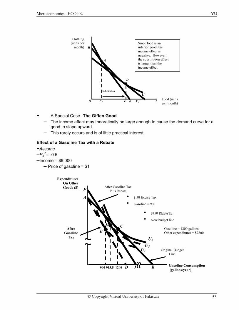
A Special Case--The Giffen Good – The income effect may theoretically be large enough to cause the demand curve for a
good to slope upward. – This rarely occurs and is of little practical interest.
Effect of a Gasoline Tax with a Rebate Assume
–Ped = -0.5
–Income = $9,000 – Price of gasoline = $1
Food (units per month)
O
R
Clothing (units per
month)
F1 S F2 T
A
U1
E
Substitution Effect
D
Since food is an inferior good, the income effect is negative. However, the substitution effect is larger than the income effect.
Gasoline Consumption (gallons/year)
Expenditures On Other Goods ($)
A
C Gasoline = 1200 gallons Other expenditures = $7800
U2
1200
Original Budget Line
BD
U1
900
After Gasoline
Tax E
• $.50 Excise Tax
• Gasoline = 900
J
F
H
913.5
After Gasoline Tax Plus Rebate
U3
• $450 REBATE
• New budget line
Microeconomics –ECO402 VU
© Copyright Virtual University of Pakistan 54
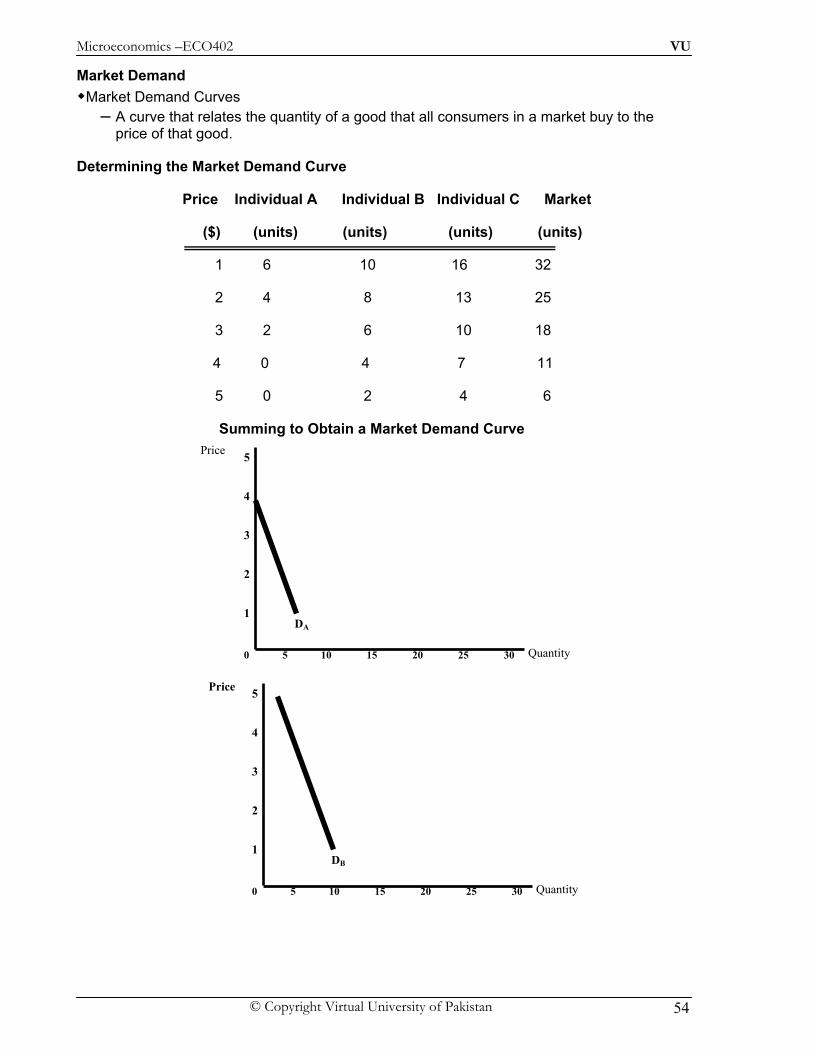
Market Demand Market Demand Curves
– A curve that relates the quantity of a good that all consumers in a market buy to the price of that good.
Determining the Market Demand Curve
Price Individual A Individual B Individual C Market
($) (units) (units) (units) (units)
1 6 10 16 32
2 4 8 13 25
3 2 6 10 18
4 0 4 7 11
5 0 2 4 6
Summing to Obtain a Market Demand Curve
Quantity
1
2
3
4
Price
0
5
5 10 15 20 25 30
DB
Quantity
1
2
3
4
Price
0
5
5 10 15 20 25 30
DA
Microeconomics –ECO402 VU
© Copyright Virtual University of Pakistan 55
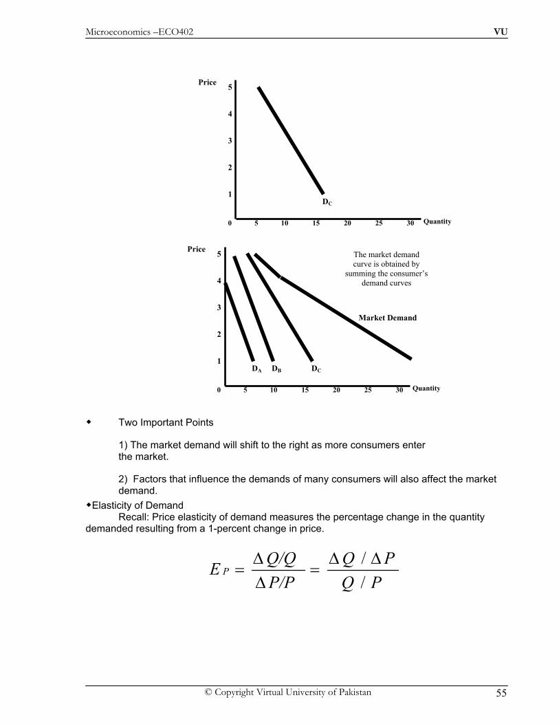
Two Important Points
1) The market demand will shift to the right as more consumers enter the market.
2) Factors that influence the demands of many consumers will also affect the market demand.
Elasticity of Demand Recall: Price elasticity of demand measures the percentage change in the quantity demanded resulting from a 1-percent change in price.
Quantity
1
2
3
4
Price
0
5
5 10 15 20 25 30
DC
Quantity
1
2
3
4
Price
0
5
5 10 15 20 25 30
DB DCDA
Market Demand
The market demand curve is obtained by
summing the consumer’s demand curves
PQPQ
P/PQ/Q E P
// ΔΔ
=ΔΔ
=
Microeconomics –ECO402 VU
© Copyright Virtual University of Pakistan 56
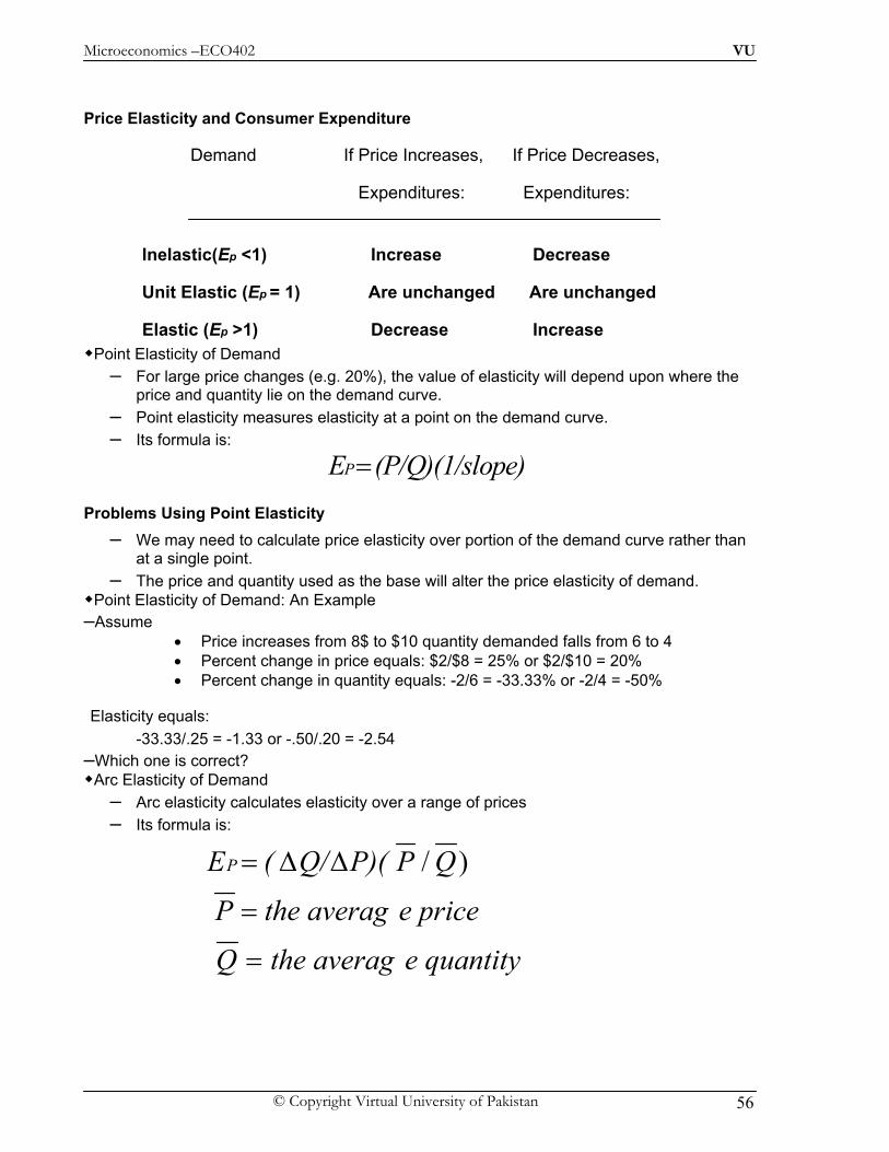
Price Elasticity and Consumer Expenditure
Demand If Price Increases, If Price Decreases,
Expenditures: Expenditures:
Inelastic(Ep <1) Increase Decrease
Unit Elastic (Ep = 1) Are unchanged Are unchanged
Elastic (Ep >1) Decrease Increase Point Elasticity of Demand
– For large price changes (e.g. 20%), the value of elasticity will depend upon where the price and quantity lie on the demand curve.
– Point elasticity measures elasticity at a point on the demand curve. – Its formula is:
P E (P/Q)(1/slope)=
Problems Using Point Elasticity – We may need to calculate price elasticity over portion of the demand curve rather than
at a single point. – The price and quantity used as the base will alter the price elasticity of demand.
Point Elasticity of Demand: An Example –Assume
• Price increases from 8$ to $10 quantity demanded falls from 6 to 4 • Percent change in price equals: $2/$8 = 25% or $2/$10 = 20% • Percent change in quantity equals: -2/6 = -33.33% or -2/4 = -50%
Elasticity equals: -33.33/.25 = -1.33 or -.50/.20 = -2.54 –Which one is correct?
Arc Elasticity of Demand – Arc elasticity calculates elasticity over a range of prices – Its formula is:
e quantitythe averagQ
e pricethe averagP
QPP)(Q/( E P
=
=
ΔΔ=
)/

Microeconomics –ECO402 VU
© Copyright Virtual University of Pakistan 57
Arc Elasticity of Demand: An Example
8.1)5/9)($2$/2(
52/10&92/184,6,10,8
)/2121
−=−=====
====ΔΔ=
pEQP
QQPPQPP)(Q/( E P
Microeconomics –ECO402 VU
© Copyright Virtual University of Pakistan 58
Lesson 12
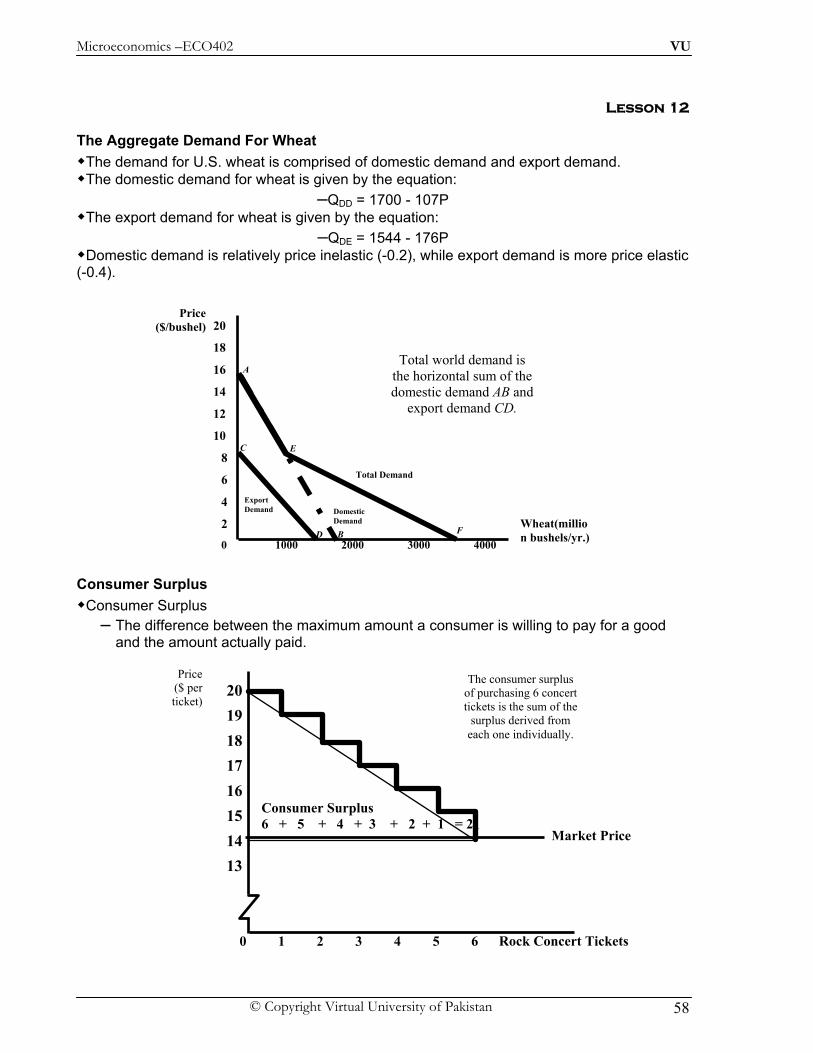
The Aggregate Demand For Wheat The demand for U.S. wheat is comprised of domestic demand and export demand. The domestic demand for wheat is given by the equation:
–QDD = 1700 - 107P The export demand for wheat is given by the equation:
–QDE = 1544 - 176P Domestic demand is relatively price inelastic (-0.2), while export demand is more price elastic
(-0.4).
Consumer Surplus Consumer Surplus
– The difference between the maximum amount a consumer is willing to pay for a good and the amount actually paid.
The consumer surplus of purchasing 6 concert tickets is the sum of the
surplus derived from each one individually.
Consumer Surplus 6 + 5 + 4 + 3 + 2 + 1 = 21
Rock Concert Tickets
Price ($ per ticket)
2 3 4 5 6
13
0 1
14 15 16 17 18 19 20
Market Price
C
D
Export Demand
A
B
Domestic Demand
Total world demand is the horizontal sum of the domestic demand AB and
export demand CD.
F
Total Demand
E
Wheat(million bushels/yr.)
Price ($/bushel)
0
2
4
6
8
10
12
14
16
18
20
1000 2000 3000 4000

Microeconomics –ECO402 VU
© Copyright Virtual University of Pakistan 59
The stepladder demand curve can be converted into a straight-line demand curve by making the units of the good smaller.
Combining consumer surplus with the aggregate profits that producers obtain we can evaluate:
1) Costs and benefits of different market structures
2) Public policies that alter the behavior of consumers and firms
An Example: The Value of Clean Air Air is free in the sense that we don’t pay to breathe it. Question: Are the benefits of cleaning up the air worth the costs? People pay more to buy houses where the air is clean. Data for house prices among neighborhoods of Lahore and Rawalpindi were compared with
the various air pollutants.
The shaded area gives the consumer surplus generated
when air pollution is reduced by 5 parts per 100 million of nitrous oxide at
a cost of $1000 per part reduced.
2000
100
1000
5
A
NOX (pphm)Pollution
Reduction
($Value per puma
of reduction)
Demand
Consumer Surplus
Actual Expenditur
$19,50014)x6,5001/2x(20 =−
Consumer Surplusfor the Market Demand
Rocket concert tickets
Price ($ per ticket)
2 3 4 5 6
13
0 1
14 15 16 17 18 19 20
Market
Microeconomics –ECO402 VU
© Copyright Virtual University of Pakistan 60
NETWORK EXTERNALITIES Up to this point we have assumed that people’s demands for a good are independent of one
another. If fact, a person’s demand may be affected by the number of other people who have
purchased the good. If this is the case, a network externality exists. Network externalities can be positive or negative. A positive network externality exists if the quantity of a good demanded by a consumer
increases in response to an increase in purchases by other consumers. Negative network externalities are just the opposite.
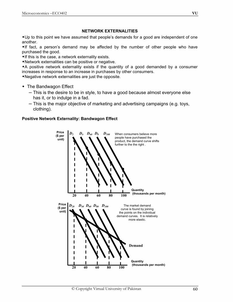
The Bandwagon Effect
– This is the desire to be in style, to have a good because almost everyone else has it, or to indulge in a fad.
– This is the major objective of marketing and advertising campaigns (e.g. toys, clothing).
Positive Network Externality: Bandwagon Effect
Quantity (thousands per month)
Price ($ per
unit)
D2
20 40
When consumers believe more people have purchased the product, the demand curve shifts further to the the right .
D4
60
D60
80
D8
100
D100
Demand
Quantity (thousands per month)
Price ($ per
unit)
D20
20 40 60 80 100
D40 D60 D80 D100 The market demand curve is found by joining
the points on the individual demand curves. It is relatively
more elastic.

Microeconomics –ECO402 VU
© Copyright Virtual University of Pakistan 61
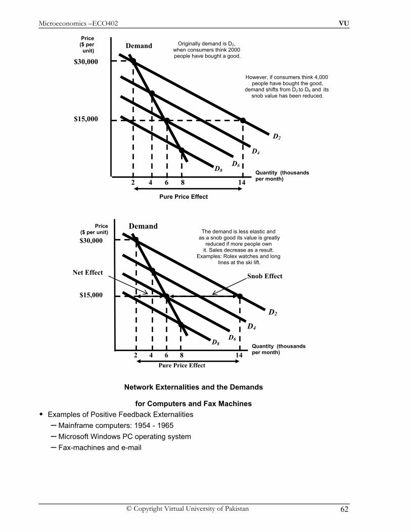
The Snob Effect – If the network externality is negative, a snob effect exists.
The snob effect refers to the desire to own exclusive or unique goods. The quantity demanded of a “snob” good is higher the fewer the people who own it.
Demand
Quantity (thousands per month)
Price ($ per
unit) D20
20 40 60 80 100
D40 D60 D80 D100
Pure Price Effect
48
Suppose the price falls from $30 to $20. If there
were no bandwagon effect, quantity demanded would only increase to 48,000
$20
$30
Demand
Quantity (thousands per month)
Price ($ per
unit) D20
20 40 60 80 100
D40 D60 D80 D100
Pure Price Effect
$20
48
Bandwagon Effect
But as more people buy the good, it becomes stylish to own it and
the quantity demanded increases further.
$30
Microeconomics –ECO402 VU
© Copyright Virtual University of Pakistan 62
Network Externalities and the Demands
for Computers and Fax Machines Examples of Positive Feedback Externalities
– Mainframe computers: 1954 - 1965 – Microsoft Windows PC operating system – Fax-machines and e-mail
Quantity (thousands per month)
Price ($ per
unit) Demand
2
D2
$30,000
$15,000
14
Pure Price Effect
Originally demand is D2, when consumers think 2000 people have bought a good.
4 6 8
D4
D6D8
However, if consumers think 4,000 people have bought the good,
demand shifts from D2 to D6 and its snob value has been reduced.
Quantity (thousands per month) 2 4 6 8
The demand is less elastic and as a snob good its value is greatly
reduced if more people own it. Sales decrease as a result.
Examples: Rolex watches and long lines at the ski lift.
Price ($ per unit)
D2
$30,000
$15,000
14
D4
D6D8
Demand
Pure Price Effect
Snob EffectNet Effect

Microeconomics –ECO402 VU
© Copyright Virtual University of Pakistan 63
Lesson 13
Introduction Choice with certainty is reasonably straightforward. How do we choose when certain variables such as income and prices are uncertain (i.e.
making choices with risk)?
Describing Risk To measure risk we must know:
1) All of the possible outcomes.
2) The likelihood that each outcome will occur (its probability). Interpreting Probability
– The likelihood that a given outcome will occur – Objective Interpretation
• Based on the observed frequency of past events – Subjective
• Based on perception or experience with or without an observed frequency – Different information or different abilities to process the same information can
influence the subjective probability Expected Value
– The weighted average of the payoffs or values resulting from all possible outcomes. • The probabilities of each outcome are used as weights • Expected value measures the central tendency; the payoff or value expected on
average – An Example
• Investment in drilling exploration: • Two outcomes are possible
– Success -- the stock price increase from $30 to $40/share – Failure -- the stock price falls from $30 to $20/share
• Objective Probability – 100 explorations, 25 successes and 75 failures – Probability (Pr) of success = 1/4 and the probability of failure = 3/4
EV Pr(success)($40/share) Pr(failure)($20/share)= +
E V 1 4 ( $ 4 0 / s h a r e ) 3 4 ( $ 2 0 / s h a r e )= +
E V $ 2 5 /sh are= Given:
– Two possible outcomes having payoffs X1 and X2
– Probabilities of each outcome is given by Pr1 & Pr2 Generally, expected value is written as:
1 1 2 2 n nE(X) PrX Pr X ... Pr X= + + +

Microeconomics –ECO402 VU
© Copyright Virtual University of Pakistan 64
Variability
– The extent to which possible outcomes of an uncertain event may differ Variability: A Scenario
– Suppose you are choosing between two part-time sales jobs that have the same expected income ($1,500)
– The first job is based entirely on commission. – The second is a salaried position. – There are two equally likely outcomes in the first job--$2,000 for a good sales job and
$1,000 for a modestly successful one. – The second pays $1,510 most of the time (.99 probability), but you will earn $510 if the
company goes out of business (.01 probability).
Income from Sales Jobs
Outcome 1 Outcome 2
Probability Income($) probability Income($) Expected income
Job 1: Commission .5 2000 .5 1000 1500
Job 2: Fixed salary .99 1510 .01 510 1500
Job 2 Expected Income
While the expected values are the same, the variability is not. Greater variability from expected values signals greater risk. Deviation
– Difference between expected payoff and actual payoff
Deviations from Expected Income ($) Outcome 1 Deviation Outcome 2 Deviation
Job 1 $2,000 $500 $1,000 -$500
Job 2 1,510 10 510 -900
– Adjusting for negative numbers
– The standard deviation measures the square root of the average of the squares of the deviations of the payoffs associated with each outcome from their expected value.
– The standard deviation is written:
1500$ .5($1000).5($2000))E(X1 =+=
$1500.01($510).99($1510) )E(X2 =+=
[ ] [ ]222
211 )(Pr)(Pr XEXXEX −+−=σ

Microeconomics –ECO402 VU
© Copyright Virtual University of Pakistan 65
Calculating Variance ($)
Deviation Deviation Deviation Standard Outcome 1 Squared Outcome 2 Squared Squared Deviation
Job 1 $2,000 $250,000 $1,000 $250,000 $250,000 $500.00
Job 2 1,510 100 510 980,100 9,900 99.50 The standard deviations of the two jobs are:
The standard deviation can be used when there are many outcomes instead of only two. An Example
– Job 1 is a job in which the income ranges from $1000 to $2000 in increments of $100 that are all equally likely.
– Job 2 is a job in which the income ranges from $1300 to $1700 in increments of $100 that, also, are all equally likely.
Outcome Probabilities of Two Jobs (unequal probability of outcomes) – Job 1: greater spread & standard deviation
50.99900,9$
00).01($980,1.99($100
500000,250$
0.5($250,000).5($250,00
2
2
2
1
1
1
==
+=
==
+=
σσ
σ
σσ
σ
*Greater Risk
Income
0.1
$1000 $1500 $2000
0.2
Job 1
Job 2
Job 1 has greater spread: greater standard deviation and greater risk than Job 2.
Probability
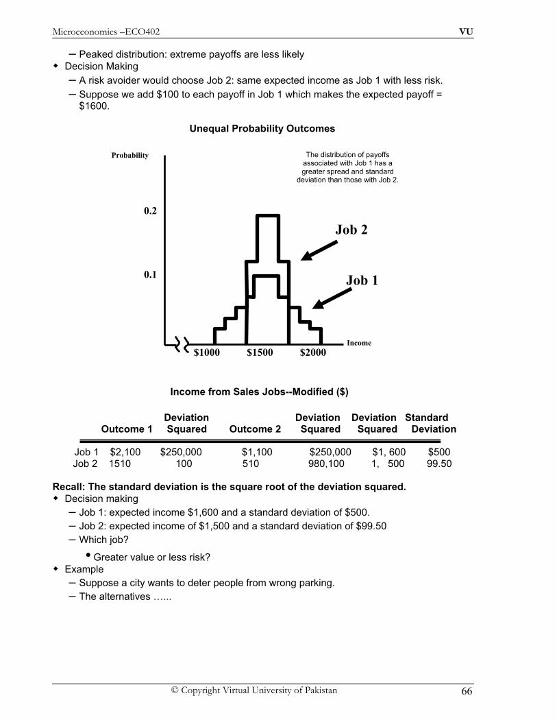
Microeconomics –ECO402 VU
© Copyright Virtual University of Pakistan 66
– Peaked distribution: extreme payoffs are less likely Decision Making
– A risk avoider would choose Job 2: same expected income as Job 1 with less risk. – Suppose we add $100 to each payoff in Job 1 which makes the expected payoff =
$1600.
Unequal Probability Outcomes
Income from Sales Jobs--Modified ($)
Deviation Deviation Deviation Standard Outcome 1 Squared Outcome 2 Squared Squared Deviation
Job 1 $2,100 $250,000 $1,100 $250,000 $1, 600 $500 Job 2 1510 100 510 980,100 1, 500 99.50
Recall: The standard deviation is the square root of the deviation squared.
Decision making – Job 1: expected income $1,600 and a standard deviation of $500. – Job 2: expected income of $1,500 and a standard deviation of $99.50 – Which job?
• Greater value or less risk? Example
– Suppose a city wants to deter people from wrong parking. – The alternatives …...
Job 1
Job 2
The distribution of payoffs associated with Job 1 has a greater spread and standard
deviation than those with Job 2.
Income
0.1
$1000 $1500 $2000
0.2
Probability

Microeconomics –ECO402 VU
© Copyright Virtual University of Pakistan 67
Assumptions:
1) Wrong parking saves a person $5 in terms of time spent searching for a parking space.
2) The driver is risk neutral.
3) Cost of apprehension is zero. A fine of $5.01 would deter the driver from double parking.
– Benefit of wrong parking ($5) is less than the cost ($5.01) equals a net benefit that is less than 0.
Increasing the fine can reduce enforcement cost: – A $50 fine with a .1 probability of being caught results in an expected penalty of $5. – A $500 fine with a .01 probability of being caught results in an expected penalty of $5.
The more risk averse drivers are, the lower the fine needs to be in order to be effective.

Microeconomics –ECO402 VU
© Copyright Virtual University of Pakistan 68
Lesson 14
PREFERENCES TOWARD RISK Choosing Among Risky Alternatives
– Assume – Consumption of a single commodity – The consumer knows all probabilities – Payoffs measured in terms of utility – Utility function given
Example – A person is earning $15,000 and receiving 13 units of utility from the job. – She is considering a new, but risky job.
She has a .50 chance of increasing her income to $30,000 and a .50 chance of decreasing her income to $10,000.
She will evaluate the position by calculating the expected value (utility) of the resulting income.
The expected utility of the new position is the sum of the utilities associated with all her possible incomes weighted by the probability that each income will occur.
The expected utility can be written: – E(u) = (1/2)u($10,000) + (1/2)u($30,000)
= 0.5(10) + 0.5(18) = 14
– E(u) of new job is 14 which is greater than the current utility of 13 and therefore preferred.
Different Preferences Toward Risk
– People can be • Risk averse • Risk neutral or • Risk loving
– Risk Averse: – A person who prefers a certain given income to a risky income with the same expected
value. – A person is considered risk averse if they have a diminishing marginal utility of income
– The use of insurance demonstrates risk aversive behavior. Risk Averse: A Scenario
– A person can have a $20,000 job with 100% probability and receive a utility level of 16. – The person could have a job with a .5 chance of earning $30,000 and a .5 chance of
earning $10,000. Expected Income =
(0.5)($30,000) + (0.5) ($10,000) = $20,000 Expected income from both jobs is the same -- risk averse may choose current job The expected utility from the new job is found:
– E(u) = (1/2)u ($10,000) + (1/2)u($30,000) – E(u) = (0.5)(10) + (0.5)(18) = 14
– E(u) of Job 1 is 16 which is greater than the E(u) of Job 2 which is 14.
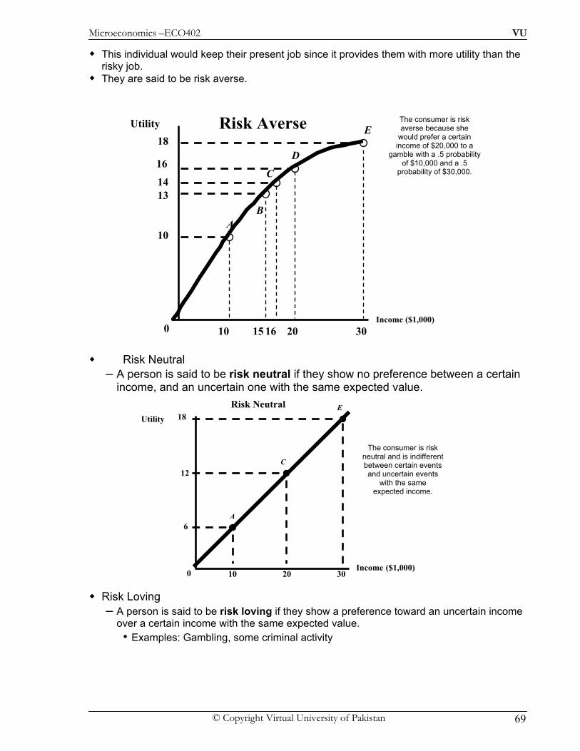
Microeconomics –ECO402 VU
© Copyright Virtual University of Pakistan 69
This individual would keep their present job since it provides them with more utility than the risky job.
They are said to be risk averse.
Risk Neutral – A person is said to be risk neutral if they show no preference between a certain
income, and an uncertain one with the same expected value.
Risk Loving – A person is said to be risk loving if they show a preference toward an uncertain income
over a certain income with the same expected value. • Examples: Gambling, some criminal activity
Income ($1,000)
Utility The consumer is risk averse because she
would prefer a certain income of $20,000 to a
gamble with a .5 probability of $10,000 and a .5
probability of $30,000.
E
10
10 15 20
13 14
16
18
0 16 30
AB
C
D
Risk Averse
Income ($1,000) 10 20
Utility
0 30
6 A
E
C 12
18
The consumer is risk neutral and is indifferent between certain events and uncertain events
with the same expected income.
Risk Neutral
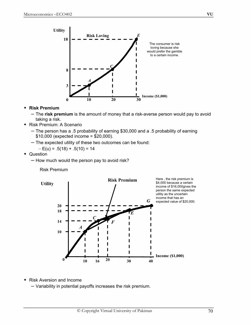
Microeconomics –ECO402 VU
© Copyright Virtual University of Pakistan 70
Risk Premium – The risk premium is the amount of money that a risk-averse person would pay to avoid
taking a risk. Risk Premium: A Scenario
– The person has a .5 probability of earning $30,000 and a .5 probability of earning $10,000 (expected income = $20,000).
– The expected utility of these two outcomes can be found: – E(u) = .5(18) + .5(10) = 14
Question – How much would the person pay to avoid risk?
Risk Aversion and Income – Variability in potential payoffs increases the risk premium.
Utility
0
3
10 20 30
A
E
C8
18 The consumer is risk loving because she
would prefer the gamble to a certain income.
Risk Loving
Income ($1,000)
Income ($1,000)
Utility
0
Risk Premium
10 16
Here , the risk premium is $4,000 because a certain income of $16,000gives the person the same expected utility as the uncertain income that has an expected value of $20,000.
10
18
30 40
20
14 A
C E
G
20
F
Risk Premium
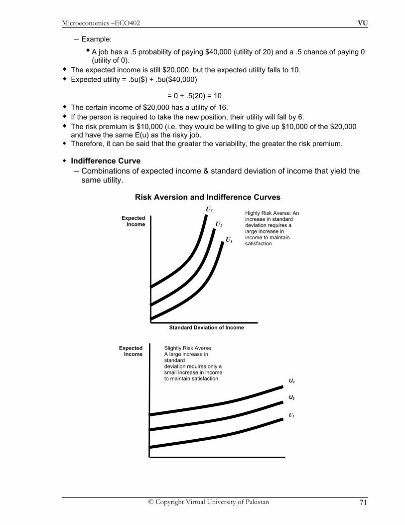
Microeconomics –ECO402 VU
© Copyright Virtual University of Pakistan 71
– Example:
• A job has a .5 probability of paying $40,000 (utility of 20) and a .5 chance of paying 0 (utility of 0).
The expected income is still $20,000, but the expected utility falls to 10. Expected utility = .5u($) + .5u($40,000)
= 0 + .5(20) = 10 The certain income of $20,000 has a utility of 16. If the person is required to take the new position, their utility will fall by 6. The risk premium is $10,000 (i.e. they would be willing to give up $10,000 of the $20,000 and have the same E(u) as the risky job.
Therefore, it can be said that the greater the variability, the greater the risk premium.
Indifference Curve – Combinations of expected income & standard deviation of income that yield the
same utility.
Risk Aversion and Indifference Curves
Expected Income
Highly Risk Averse: An increase in standard deviation requires a large increase in income to maintain satisfaction.
U1
U2
U3
Standard Deviation of Income
Expected Income
Slightly Risk Averse: A large increase in standard deviation requires only a small increase in income to maintain satisfaction.
U1
U2
U3
Microeconomics –ECO402 VU
© Copyright Virtual University of Pakistan 72
Business Executives and the Choice of Risk Example
– Study of 464 executives found that:
• 20% were risk neutral
• 40% were risk takers
• 20% were risk averse
• 20% did not respond Those who liked risky situations did so when losses were involved. When risks involved gains the same, executives opted for less risky situations. The executives made substantial efforts to reduce or eliminate risk by delaying decisions
and collecting more information.
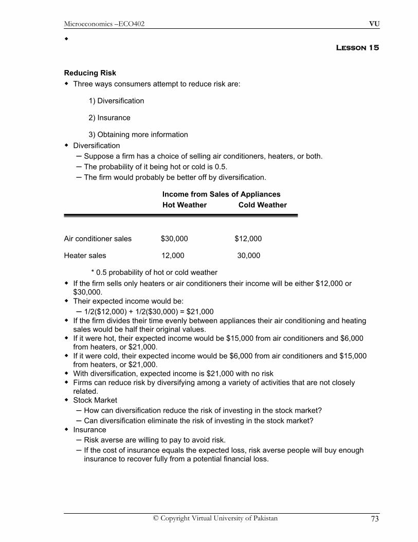
Microeconomics –ECO402 VU
© Copyright Virtual University of Pakistan 73
Lesson 15
Reducing Risk Three ways consumers attempt to reduce risk are:
1) Diversification
2) Insurance
3) Obtaining more information Diversification
– Suppose a firm has a choice of selling air conditioners, heaters, or both. – The probability of it being hot or cold is 0.5. – The firm would probably be better off by diversification.
Income from Sales of Appliances Hot Weather Cold Weather
Air conditioner sales $30,000 $12,000
Heater sales 12,000 30,000
* 0.5 probability of hot or cold weather If the firm sells only heaters or air conditioners their income will be either $12,000 or
$30,000. Their expected income would be:
– 1/2($12,000) + 1/2($30,000) = $21,000 If the firm divides their time evenly between appliances their air conditioning and heating
sales would be half their original values. If it were hot, their expected income would be $15,000 from air conditioners and $6,000
from heaters, or $21,000. If it were cold, their expected income would be $6,000 from air conditioners and $15,000
from heaters, or $21,000. With diversification, expected income is $21,000 with no risk Firms can reduce risk by diversifying among a variety of activities that are not closely
related. Stock Market
– How can diversification reduce the risk of investing in the stock market? – Can diversification eliminate the risk of investing in the stock market?
Insurance – Risk averse are willing to pay to avoid risk. – If the cost of insurance equals the expected loss, risk averse people will buy enough
insurance to recover fully from a potential financial loss.
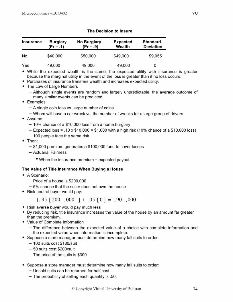
Microeconomics –ECO402 VU
© Copyright Virtual University of Pakistan 74
The Decision to Insure Insurance Burglary No Burglary Expected Standard (Pr = .1) (Pr = .9) Wealth Deviation
No $40,000 $50,000 $49,000 $9,055
Yes 49,000 49,000 49,000 0 While the expected wealth is the same, the expected utility with insurance is greater
because the marginal utility in the event of the loss is greater than if no loss occurs. Purchases of insurance transfers wealth and increases expected utility. The Law of Large Numbers
– Although single events are random and largely unpredictable, the average outcome of many similar events can be predicted.
Examples – A single coin toss vs. large number of coins – Whom will have a car wreck vs. the number of wrecks for a large group of drivers
Assume: – 10% chance of a $10,000 loss from a home burglary – Expected loss = .10 x $10,000 = $1,000 with a high risk (10% chance of a $10,000 loss) – 100 people face the same risk
Then: – $1,000 premium generates a $100,000 fund to cover losses – Actuarial Fairness
• When the insurance premium = expected payout
The Value of Title Insurance When Buying a House A Scenario:
– Price of a house is $200,000 – 5% chance that the seller does not own the house
Risk neutral buyer would pay:
Risk averse buyer would pay much less By reducing risk, title insurance increases the value of the house by an amount far greater
than the premium. Value of Complete Information
– The difference between the expected value of a choice with complete information and the expected value when information is incomplete.
Suppose a store manager must determine how many fall suits to order: – 100 suits cost $180/suit – 50 suits cost $200/suit – The price of the suits is $300
Suppose a store manager must determine how many fall suits to order:
– Unsold suits can be returned for half cost. – The probability of selling each quantity is .50.
000,190]0[05.]000,200[95(. =+

Microeconomics –ECO402 VU
© Copyright Virtual University of Pakistan 75
The Decision to Insure Expected
Sale of 50 Sale of 100 Profit
1. Buy 50 suits $5,000 $5,000 $5,000
2. Buy 100 suits 1,500 12,000 6,750
With incomplete information: – Risk Neutral: Buy 100 suits – Risk Averse: Buy 50 suits
The expected value with complete information is $8,500. – 8,500 = .5(5,000) + .5(12,000)
The expected value with uncertainty (buy 100 suits) is $6,750. The value of complete information is $1,750, or the difference between the two (the amount
the store owner would be willing to pay for a marketing study). An Example
– Per capita packed milk consumption has fallen over the years – The milk producers engaged in market research to develop new sales strategies to
encourage the consumption of packed milk. Findings
– Packed milk demand is seasonal with the greatest demand in the summer – Ep is negative and small – EI is positive and large
Milk advertising increases sales most in the summer. Allocating advertising based on this information in Karachi increased sales by Rs. 400,000
and profits by 9%. The cost of the information was relatively low, while the value was substantial.
The Demand for Risky Assets Assets
– Something that provides a flow of money or services to its owner. – The flow of money or services can be explicit (dividends) or implicit (capital gain).
Capital Gain – An increase in the value of an asset, while a decrease is a capital loss.
Risky & Riskless Assets – Risky Asset
• Provides an uncertain flow of money or services to its owner.
• Examples – Apartment rent, capital gains, corporate bonds, stock prices
– Riskless Asset
• Provides a flow of money or services that is known with certainty.
• Examples – Short-term government bonds, short-term certificates of deposit

Microeconomics –ECO402 VU
© Copyright Virtual University of Pakistan 76
Asset Returns – Return on an Asset
– The total monetary flow of an asset as a fraction of its price. – Real Return of an Asset
– The simple (or nominal) return less the rate of inflation. Asset Returns
Monetary FlowAsset Return
Purchase Price=
Flow $100/yr.Asset Return 10%
Bond Price $1,000= = =
Expected vs. Actual Returns – Expected Return
• Return that an asset should earn on average – Actual Return
• Return that an asset earns – Higher returns are associated with greater risk. – The risk-averse investor must balance risk relative to return
Risk and Budget Line
Expected return, RP, increases as risk increases.
The slope is the price of risk or the risk-return trade-off.
Choosing Between Risk and Return
0
Expected Return, Rp
U2 is the optimal choice of those obtainable, since it gives the highest return for a given risk and is tangent to the budget
line.
Rf
Budget Line
mσ
Rm
∗σ
R*
U2U1
U3
σ* σm Standard Deviation of Return, σp
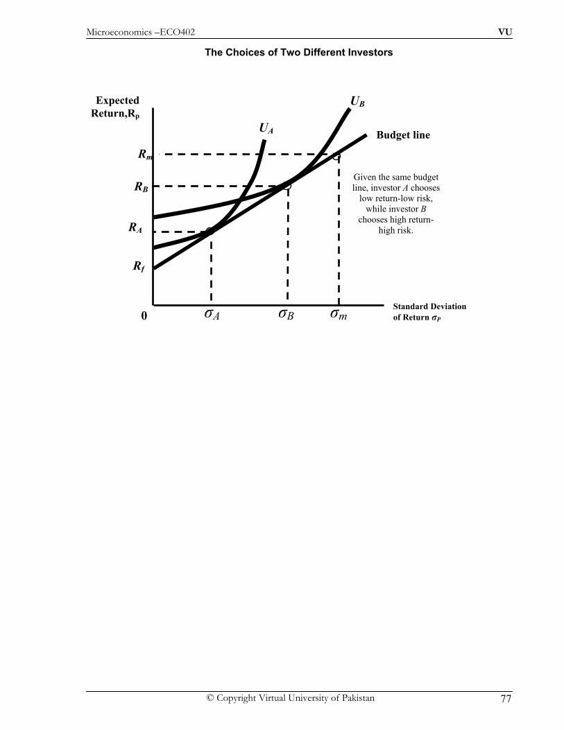
Microeconomics –ECO402 VU
© Copyright Virtual University of Pakistan 77
The Choices of Two Different Investors
Rf
Budget line
0
Expected Return,Rp
Given the same budget line, investor A chooses
low return-low risk, while investor B
chooses high return- high risk.
UA
RA
UB
RB
Rm
Standard Deviation of Return σP σA σB σm

Microeconomics –ECO402 VU
© Copyright Virtual University of Pakistan 78
Lesson 16
Introduction Our focus is the supply side. The theory of the firm will address:
– How a firm makes cost-minimizing production decisions – How cost varies with output – Characteristics of market supply
The Technology of Production The Production Process
– Combining inputs or factors of production to achieve an output Categories of Inputs (factors of production)
– Labor – Materials – Capital
Production Function: – Indicates the highest output that a firm can produce for every specified combination of
inputs given the state of technology. – Shows what is technically feasible when the firm operates efficiently.
The production functions for two inputs:
Q = F(K,L)
Q = Output, K = Capital, L = Labor For a given technology
Isoquants Assumptions
– Food producer has two inputs
• Labor (L) & Capital (K) Observations:
1) For any level of K, output increases with more L.
2) For any level of L, output increases with more K.
3) Various combinations of inputs produce the same output. Isoquants
– Curves showing all possible combinations of inputs that yield the same output
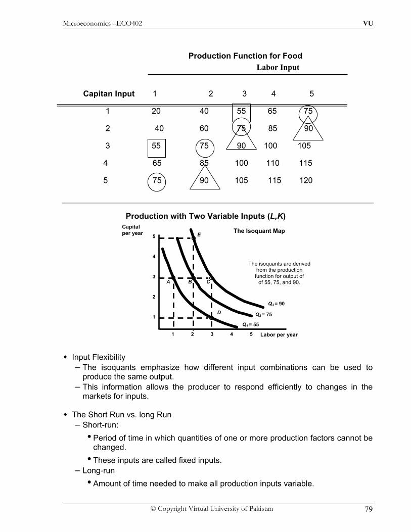
Microeconomics –ECO402 VU
© Copyright Virtual University of Pakistan 79
Production Function for Food Labor Input
Capitan Input 1 2 3 4 5
1 20 40 55 65 75
2 40 60 75 85 90
3 55 75 90 100 105
4 65 85 100 110 115
5 75 90 105 115 120
Production with Two Variable Inputs (L,K)
Input Flexibility – The isoquants emphasize how different input combinations can be used to
produce the same output. – This information allows the producer to respond efficiently to changes in the
markets for inputs.
The Short Run vs. long Run – Short-run:
• Period of time in which quantities of one or more production factors cannot be changed.
• These inputs are called fixed inputs. – Long-run
• Amount of time needed to make all production inputs variable.
Labor per year
1
2
3
4
1 2 3 4 5
5
Q1 = 55
The isoquants are derived from the production function for output of
of 55, 75, and 90. A
D
B
Q2 = 75
Q3 = 90
C
ECapital per year The Isoquant Map

Microeconomics –ECO402 VU
© Copyright Virtual University of Pakistan 80
Production with One Variable Input (Labor) Amount Amount Total Average Marginal of Labor (L) of Capital (K) Output (Q) Product Product
0 10 0 --- ---
1 10 10 10 10
2 10 30 15 20
3 10 60 20 30
4 10 80 20 20
5 10 95 19 15
6 10 108 18 13
7 10 112 16 4
8 10 112 14 0
9 10 108 12 -4
10 10 100 10 -8 Observations:
1) With additional workers, output (Q) increases, reaches a maximum, and then decreases.
2) The average product of labor (AP), or output per worker, increases and then decreases. 3) The marginal product of labor (MP), or output of the additional worker, increases rapidly initially and then decreases and becomes negative..
LQ
Input LaborOutput AP ==
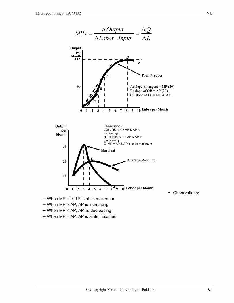
Microeconomics –ECO402 VU
© Copyright Virtual University of Pakistan 81
Observations: – When MP = 0, TP is at its maximum – When MP > AP, AP is increasing – When MP < AP, AP is decreasing – When MP = AP, AP is at its maximum
Total Product
A: slope of tangent = MP (20) B: slope of OB = AP (20) C: slope of OC= MP & AP
Labor per Month
Output per
Month
60
112
0 2 3 4 5 6 7 8 9 101
A
B
C
D
LQ
Input LaborOutput MP L
ΔΔ
=Δ
Δ=
Average Product
8
10
20
Output per
Month
0 2 3 4 5 6 7 9 101 Labor per Month
30
E
Marginal
Observations: Left of E: MP > AP & AP is increasing Right of E: MP < AP & AP is decreasing E: MP = AP & AP is at its maximum

Microeconomics –ECO402 VU
© Copyright Virtual University of Pakistan 82
AP = slope of line from origin to a point on TP, lines b, & c. MP = slope of a tangent to any point on the TP line, lines a & c.
The Law of Diminishing Marginal Returns
– As the use of an input increases in equal increments, a point will be reached at which the resulting additions to output decreases (i.e. MP declines).
– When the labor input is small, MP increases due to specialization. – When the labor input is large, MP decreases due to inefficiencies.
The Law of Diminishing Marginal Returns – Can be used for long-run decisions to evaluate the trade-offs of different plant
configurations – Assumes the quality of the variable input is constant – Explains a declining MP, not necessarily a negative one – Assumes a constant technology
The Effect of Technological Improvement
Laborper Month
Output per
Month
60
112
0 2 3 4 5 6 7 8 9 101
A
B
C
D
8
10
20E
0 2 3 4 5 6 7 9 10 1
30
Outputper
Month
Labor per Month
Labor pertime period
Output per
time period
50
100
0 2 3 4 5 6 7 8 9 101
A
O1
C
O3
O2
B
Labor productivity can increase if there are improvements in
technology, even though any given production
process exhibits diminishing returns to
labor.
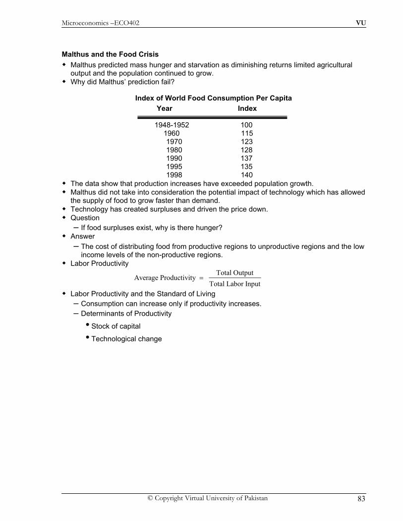
Microeconomics –ECO402 VU
© Copyright Virtual University of Pakistan 83
Malthus and the Food Crisis Malthus predicted mass hunger and starvation as diminishing returns limited agricultural
output and the population continued to grow. Why did Malthus’ prediction fail?
Index of World Food Consumption Per Capita Year Index
1948-1952 100 1960 115 1970 123 1980 128 1990 137 1995 135 1998 140
The data show that production increases have exceeded population growth. Malthus did not take into consideration the potential impact of technology which has allowed
the supply of food to grow faster than demand. Technology has created surpluses and driven the price down. Question
– If food surpluses exist, why is there hunger? Answer
– The cost of distributing food from productive regions to unproductive regions and the low income levels of the non-productive regions.
Labor Productivity Total Output
Average Productivity Total Labor Input
=
Labor Productivity and the Standard of Living – Consumption can increase only if productivity increases. – Determinants of Productivity
• Stock of capital
• Technological change
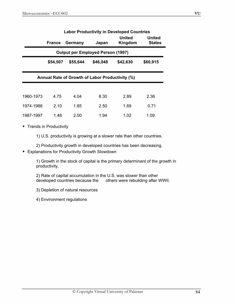
Microeconomics –ECO402 VU
© Copyright Virtual University of Pakistan 84
Labor Productivity in Developed Countries United United France Germany Japan Kingdom States
Output per Employed Person (1997)
$54,507 $55,644 $46,048 $42,630 $60,915
Annual Rate of Growth of Labor Productivity (%)
1960-1973 4.75 4.04 8.30 2.89 2.36
1974-1986 2.10 1.85 2.50 1.69 0.71
1987-1997 1.48 2.00 1.94 1.02 1.09
Trends in Productivity
1) U.S. productivity is growing at a slower rate than other countries.
2) Productivity growth in developed countries has been decreasing. Explanations for Productivity Growth Slowdown
1) Growth in the stock of capital is the primary determinant of the growth in productivity.
2) Rate of capital accumulation in the U.S. was slower than other developed countries because the others were rebuilding after WWII.
3) Depletion of natural resources
4) Environment regulations
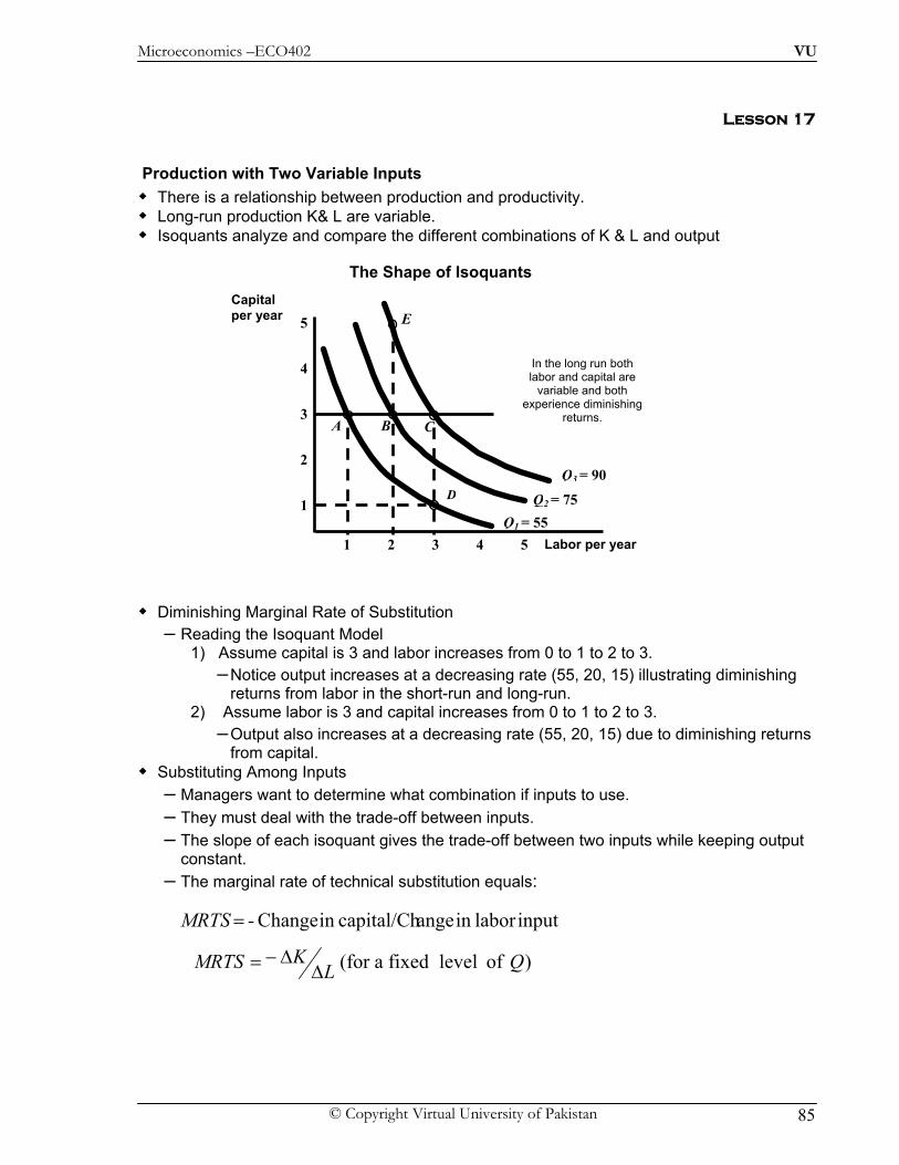
Microeconomics –ECO402 VU
© Copyright Virtual University of Pakistan 85
Lesson 17
Production with Two Variable Inputs There is a relationship between production and productivity. Long-run production K& L are variable. Isoquants analyze and compare the different combinations of K & L and output
The Shape of Isoquants
Diminishing Marginal Rate of Substitution
– Reading the Isoquant Model 1) Assume capital is 3 and labor increases from 0 to 1 to 2 to 3.
– Notice output increases at a decreasing rate (55, 20, 15) illustrating diminishing returns from labor in the short-run and long-run.
2) Assume labor is 3 and capital increases from 0 to 1 to 2 to 3. – Output also increases at a decreasing rate (55, 20, 15) due to diminishing returns
from capital. Substituting Among Inputs
– Managers want to determine what combination if inputs to use. – They must deal with the trade-off between inputs. – The slope of each isoquant gives the trade-off between two inputs while keeping output
constant. – The marginal rate of technical substitution equals:
Labor per year
1
2
3
4
1 2 3 4 5
5
In the long run both labor and capital are
variable and both experience diminishing
returns.
Q1 = 55Q2 = 75
Q3 = 90
Capital per year
A
D
B C
E
inputlabor in angecapital/Chin Change - MRTS =
) of level fixed a(for QLK MRTS Δ
Δ−=
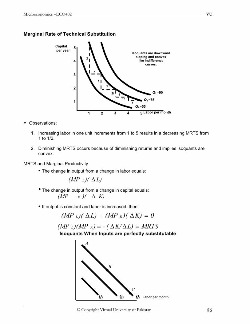
Microeconomics –ECO402 VU
© Copyright Virtual University of Pakistan 86
Marginal Rate of Technical Substitution
Observations:
1. Increasing labor in one unit increments from 1 to 5 results in a decreasing MRTS from 1 to 1/2.
2. Diminishing MRTS occurs because of diminishing returns and implies isoquants are convex.
MRTS and Marginal Productivity • The change in output from a change in labor equals:
• The change in output from a change in capital equals:
• If output is constant and labor is increased, then:
Isoquants When Inputs are perfectly substitutable
Labor per month
1
2
3
4
1 2 3 4 5
5 Capital per year
Isoquants are downwardsloping and convex
like indifference curves.
1
1
1
1
2
1
2/
1/
Q1 =55
Q2 =75
Q3 =90
L))((MP L Δ
K))((MP K Δ
0 K))((MP L))((MP KL =Δ+Δ MRTS L)K/(- ))(MP(MP KL =ΔΔ=
Labor per month Q1 Q2 Q3
A
B
C

Microeconomics –ECO402 VU
© Copyright Virtual University of Pakistan 87
Perfect Substitute Observations when inputs are perfectly substitutable:
1) The MRTS is constant at all points on the isoquant.
2) For a given output, any combination of inputs can be chosen (A, B, or C) to generate the same level of output (e.g. toll booths & musical instruments).
Fixed-Proportions Production Function Fixed-Proportions Production Function
– Observations when inputs must be in a fixed-proportion: 1) No substitution is possible. Each output requires a specific amount of each input (e.g. labor and jackhammers). 2)To increase output requires more labor and capital (i.e. moving from A to B to C which is technically efficient).
A Production Function for Wheat Farmers must choose between a capital intensive or labor intensive technique of
production.
Labor per month
Capital per
month
L1
K1 Q1
Q2
Q3
A
B
C
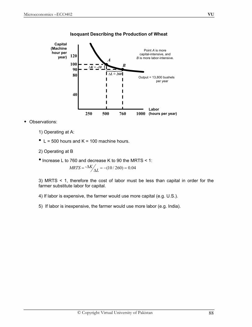
Microeconomics –ECO402 VU
© Copyright Virtual University of Pakistan 88
Isoquant Describing the Production of Wheat
Observations:
1) Operating at A:
• L = 500 hours and K = 100 machine hours.
2) Operating at B
• Increase L to 760 and decrease K to 90 the MRTS < 1: (10 / 260) 0.04- KMRTS L
Δ= = − =Δ
3) MRTS < 1, therefore the cost of labor must be less than capital in order for the farmer substitute labor for capital.
4) If labor is expensive, the farmer would use more capital (e.g. U.S.).
5) If labor is inexpensive, the farmer would use more labor (e.g. India).
Labor(hours per year)
Capital (Machine hour per
year)
250 500 760 1000
40
80
120
100 90
Output = 13,800 bushels per year
AB
Point A is more capital-intensive, and
B is more labor-intensive.
∆K = -10
∆L = 260

Microeconomics –ECO402 VU
© Copyright Virtual University of Pakistan 89
Returns to Scale Measuring the relationship between the scale (size) of a firm and output
1. Increasing returns to scale: output more than doubles when all inputs are doubled – Larger output associated with lower cost (autos) – One firm is more efficient than many (utilities) – The isoquants get closer together
2. Constant returns to scale: output doubles when all inputs are doubled. • Size does not affect productivity • May have a large number of producers • Isoquants are equidistant apart
Decreasing returns to scale: output less than doubles when all inputs are doubled
Labor (hours)
Capital (machine
hours)
10
20
30
Increasing Returns: The isoquants move closer together
5 10
2
4
0
A
Labor (hours)
Capital (machine
hours)
Constant Returns:Isoquants are equally spaced
10
20
30
15 5 10
2
4
0
A
6

Microeconomics –ECO402 VU
© Copyright Virtual University of Pakistan 90
3. Decreasing returns to scale: output less than doubles when all inputs are doubled • Decreasing efficiency with large size • Reduction of entrepreneurial abilities • Isoquants become farther apart
Returns to Scale in the Carpet Industry The carpet industry has grown from a small industry to a large industry with some very large
firms. Question
– Can the growth be explained by the presence of economies to scale?
The U.S. Carpet Industry Carpet Shipments, 1996 (Millions of Dollars per Year)
1. Shaw Industries $3,202 6. World Carpets $475
2. Mohawk Industries 1,795 7. Burlington Industries 450
3. Beaulieu of America 1,006 8. Collins & Aikman 418
4. Interface Flooring 820 9. Masland Industries 380
5. Queen Carpet 775 10. Dixied Yarns 280 Are there economies of scale?
– Costs (percent of cost)
• Capital -- 77%
• Labor -- 23% Large Manufacturers
– Increased in machinery & labor – Doubling inputs has more than doubled output – Economies of scale exist for large producers
Small Manufacturers – Small increases in scale have little or no impact on output – Proportional increases in inputs increase output proportionally
Labor (hours)
Capital (machine
hours) Decreasing Returns: Isoquants get further apart
10 20
30
5 10
2
4
0
A
Microeconomics –ECO402 VU
© Copyright Virtual University of Pakistan 91
– Constant returns to scale for small producers

Microeconomics –ECO402 VU
© Copyright Virtual University of Pakistan 92
– Lesson 18
Introduction The production technology measures the relationship between input and output. Given the production technology, managers must choose how to produce. To determine the optimal level of output and the input combinations, we must convert from
the unit measurements of the production technology to dollar measurements or costs.
Measuring Cost: Which Costs Matter? Accounting Cost vs. Economic Cost
– Accounting Cost
• Actual expenses plus depreciation charges for capital equipment – Economic Cost
• Cost to a firm of utilizing economic resources in production, including opportunity cost Opportunity cost.
– Cost associated with opportunities that are foregone when a firm’s resources are not put to their highest-value use.
An Example – A firm owns its own building and pays no rent for office space – Does this mean the cost of office space is zero?
Sunk Cost – Expenditure that has been made and cannot be recovered – Should not influence a firm’s decisions.
An Example – A firm pays $500,000 for an option to buy a building. – The cost of the building is $5 million or a total of $5.5 million. – The firm finds another building for $5.25 million. – Which building should the firm buy?
Fixed and Variable Costs – Total output is a function of variable inputs and fixed inputs. – Therefore, the total cost of production equals the fixed cost (the cost of the fixed inputs)
plus the variable cost (the cost of the variable inputs), or…
– Fixed Cost
• Does not vary with the level of output – Variable Cost
• Cost that varies as output varies Fixed Cost
– Cost paid by a firm that is in business regardless of the level of output Sunk Cost
– Cost that have been incurred and cannot be recovered Personal Computers: most costs are variable
– Components, labor Software: most costs are sunk
– Cost of developing the software
VC FC TC +=
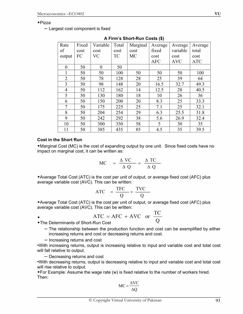
Microeconomics –ECO402 VU
© Copyright Virtual University of Pakistan 93
Pizza – Largest cost component is fixed
A Firm’s Short-Run Costs ($) Rate of output
Fixed cost FC
Variable cost VC
Total cost TC
Marginal cost MC
Average fixed cost AFC
Average variable cost AVC
Average total cost ATC
0 50 0 50 1 50 50 100 50 50 50 100 2 50 78 128 28 25 39 64 3 50 98 148 20 16.5 32.7 49.3 4 50 112 162 14 12.5 28 40.5 5 50 130 180 18 10 26 36 6 50 150 200 20 8.3 25 33.3 7 50 175 225 25 7.1 25 32.1 8 50 204 254 29 6.3 25.5 31.8 9 50 242 292 38 5.6 26.9 32.4 10 50 300 350 58 5 30 35 11 50 385 435 85 4.5 35 39.5
Cost in the Short Run Marginal Cost (MC) is the cost of expanding output by one unit. Since fixed costs have no
impact on marginal cost, it can be written as:
Average Total Cost (ATC) is the cost per unit of output, or average fixed cost (AFC) plus
average variable cost (AVC). This can be written:
Average Total Cost (ATC) is the cost per unit of output, or average fixed cost (AFC) plus average variable cost (AVC). This can be written:
The Determinants of Short-Run Cost
– The relationship between the production function and cost can be exemplified by either increasing returns and cost or decreasing returns and cost.
– Increasing returns and cost •With increasing returns, output is increasing relative to input and variable cost and total cost will fall relative to output.
– Decreasing returns and cost •With decreasing returns, output is decreasing relative to input and variable cost and total cost will rise relative to output.
For Example: Assume the wage rate (w) is fixed relative to the number of workers hired. Then:
VCMC
QΔ
=Δ
QTC
QVC MC
ΔΔ
=Δ
Δ=
QTVC
QTFC ATC +=
QTCor AVC AFC ATC +=
Microeconomics –ECO402 VU
© Copyright Virtual University of Pakistan 94
VC Lw=
LMC
QwΔ
=Δ
LMP LQΔ
Δ =Δ
L
L 1L for a 1 unit Q
Q MPΔ
Δ Δ = =Δ Δ
In conclusion:
LMC
MPw
=
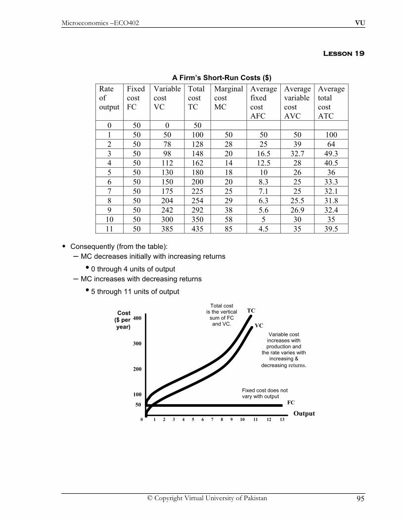
Microeconomics –ECO402 VU
© Copyright Virtual University of Pakistan 95
Lesson 19
A Firm’s Short-Run Costs ($) Rate of output
Fixed cost FC
Variable cost VC
Total cost TC
Marginal cost MC
Average fixed cost AFC
Average variable cost AVC
Average total cost ATC
0 50 0 50 1 50 50 100 50 50 50 100 2 50 78 128 28 25 39 64 3 50 98 148 20 16.5 32.7 49.3 4 50 112 162 14 12.5 28 40.5 5 50 130 180 18 10 26 36 6 50 150 200 20 8.3 25 33.3 7 50 175 225 25 7.1 25 32.1 8 50 204 254 29 6.3 25.5 31.8 9 50 242 292 38 5.6 26.9 32.4 10 50 300 350 58 5 30 35 11 50 385 435 85 4.5 35 39.5
Consequently (from the table):
– MC decreases initially with increasing returns
• 0 through 4 units of output – MC increases with decreasing returns
• 5 through 11 units of output
Output
Cost ($ per year)
100
200
300
400
0 1 2 3 4 5 6 7 8 9 10 11 12 13
VCVariable cost increases with production and
the rate varies with increasing &
decreasing returns.
TCTotal cost
is the verticalsum of FC and VC.
FC 50
Fixed cost does not vary with output

Microeconomics –ECO402 VU
© Copyright Virtual University of Pakistan 96
The line drawn from the origin to the tangent of the variable cost curve:
– Its slope equals AVC
– The slope of a point on VC equals MC
– Therefore, MC = AVC at 7 units of output (point A) Unit Costs
– AFC falls continuously
– When MC < AVC or MC < ATC, AVC & ATC decrease
– When MC > AVC or MC > ATC, AVC & ATC increase
– MC = AVC and ATC at minimum AVC and ATC
– Minimum AVC occurs at a lower output than minimum ATC due to FC
The User Cost of Capital User Cost of Capital = Economic Depreciation + (Interest Rate)(Value of Capital)
– Example
• An Airline buys a Boeing 737 for $150 million with an expected life of 30 years – Annual economic depreciation = $150 million/30 = $5 million – Interest rate = 10%
• User Cost of Capital = $5 million + (.10) ($150 million – depreciation) – Year 1 = $5 million + (.10)($150 million) = $20 million – Year 10 = $5 million + (.10) ($100 million) = $15 million
– Rate per dollar of capital
• r = Depreciation Rate + Interest Rate – Airline Example
• Depreciation Rate = 1/30 = 3.33/yr
• Rate of Return = 10%/yr – User Cost of Capital
• r = 3.33 + 10 = 13.33%/yr
Output (units/yr.)
Cost ($ per unit)
25
50
75
100
0 1 2 3 4 5 6 7 8 9 10 11
MC
ATC
AVC
AFC

Microeconomics –ECO402 VU
© Copyright Virtual University of Pakistan 97
The Cost Minimizing Input Choice – Assumptions
• Two Inputs: Labor (L) & capital (K)
• Price of labor: wage rate (w)
• The price of capital – R = depreciation rate + interest rate
– Question
• If capital was rented, would it change the value of r ? The Isocost Line
– C = wL + rK – Isocost: A line showing all combinations of L & K that can be purchased for the same
cost – Rewriting C as linear:
• K = C/r - (w/r)L
• Slope of the Isocost:
( )Δ = −ΔwK
L r
is the ratio of the wage rate to rental cost of capital. This shows the rate at which capital can be substituted for labor with no
change in cost.
Choosing Inputs • We will address how to minimize cost for a given level of output. • We will do so by combining Isocosts with Isoquants
Producing a Given Output at Minimum Cost
Labor per year
Capital per
year
Q1
Q1 is an isoquant for output Q1.
Isocost curve C0 shows all combinations of K and Lthat can not produce Q1 at
this
C0 C1 C2
CO C1 C2 arethree
Isocost lines AK1
L1
K3
L3
K2
L2
Isocost C2 shows quantity Q1 can be produced with
combination K2L2 or K3L3. However, both of these
are higher cost combinations than K1L1.

Microeconomics –ECO402 VU
© Copyright Virtual University of Pakistan 98
Input Substitution When an Input Price Change
Isoquants and Isocosts and the Production Function
LK
- MPMRTS MPK
LΔ= =Δ
Slope of isocost line wKL r
Δ= = −Δ
and L
K
MP wMP r= =
The minimum cost combination can then be written as: L KMP MP
w r=
– Minimum cost for a given output will occur when each dollar of input added to the production process will add an equivalent amount of output.
Question – If w = $10, r = $2, and MPL = MPK, which input would the producer use more of? Why?
The Effect of Effluent Fees on Firms’ Input Choices
The Effect of Effluent Fees on Firms’ Input Choices Firms that have a by-product to production produce an effluent. An effluent fee is a per-unit fee that firms must pay for the effluent that they emit. How would a producer respond to an effluent fee on production? The Scenario: Steel Producer
C2
This yields a new combination of K and L to produce Q1.
Combination B is used in place of combination A.
The new combination represents the higher cost of labor relative to capital and therefore capital
is substituted for labor.
K2
L2
B
C1
K1
L1
A
Q1
If the price of labor changes, the Isocost curve
becomes steeper due to the change in the slope -(w/L).
Labor per year
Capital per
year
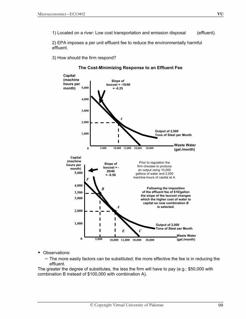
Microeconomics –ECO402 VU
© Copyright Virtual University of Pakistan 99
1) Located on a river: Low cost transportation and emission disposal (effluent).
2) EPA imposes a per unit effluent fee to reduce the environmentally harmful effluent.
3) How should the firm respond?
The Cost-Minimizing Response to an Effluent Fee
Observations: – The more easily factors can be substituted; the more effective the fee is in reducing the
effluent. The greater the degree of substitutes, the less the firm will have to pay (e.g.: $50,000 with combination B instead of $100,000 with combination A).
Waste Water (gal./month)
Capital (machine hours per month)
Output of 2,000 Tons of Steel per Month
A
10,000 18,000 20,0000 12,000
Slope of Isocost = -10/40
= -0.25
2,000
1,000
4,000
3,000
5,000
5,000
Output of 2,000 Tons of Steel per Month
2,000
1,000
4,000
3,000
5,000
10,000 18,000 20,0000 12,000
Capital (machine hours per
month)
E
5,000
3,500
Slope of Isocost = -
20/40 = -0.50
B Following the imposition of the effluent fee of $10/gallon
the slope of the Isocost changes which the higher cost of water to
capital so now combination B is selected. A
Prior to regulation the firm chooses to produce an output using 10,000
gallons of water and 2,000 machine-hours of capital at A.
C
F
Waste Water (gal./month)
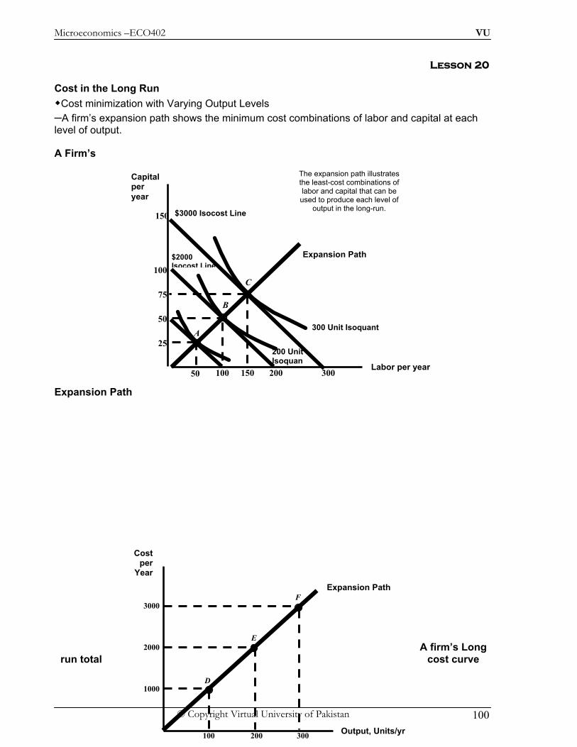
Microeconomics –ECO402 VU
© Copyright Virtual University of Pakistan 100
Lesson 20
Cost in the Long Run Cost minimization with Varying Output Levels
–A firm’s expansion path shows the minimum cost combinations of labor and capital at each level of output.
A Firm’s
Expansion Path
A firm’s Long
run total cost curve
Labor per year
Capital per year
Expansion Path
The expansion path illustrates the least-cost combinations of labor and capital that can be used to produce each level of
output in the long-run.
25
50
75
100
150
100 50 150 300200
A
$2000 Isocost Line
200 UnitIsoquan
B
$3000 Isocost Line
300 Unit Isoquant
C
Output, Units/yr
Cost per
Year
Expansion Path
1000
100 300200
2000
3000
D
E
F

Microeconomics –ECO402 VU
© Copyright Virtual University of Pakistan 101
Long-Run Versus Short-Run Cost Curves What happens to average costs when both inputs are variable (long run) versus only having
one input that is variable (short run)?
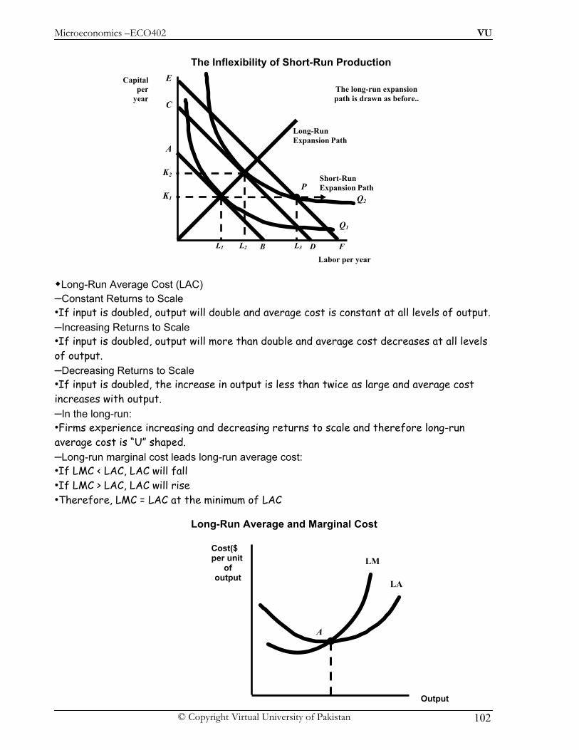
Microeconomics –ECO402 VU
© Copyright Virtual University of Pakistan 102
The Inflexibility of Short-Run Production
Long-Run Average Cost (LAC) –Constant Returns to Scale •If input is doubled, output will double and average cost is constant at all levels of output. –Increasing Returns to Scale •If input is doubled, output will more than double and average cost decreases at all levels of output. –Decreasing Returns to Scale •If input is doubled, the increase in output is less than twice as large and average cost increases with output. –In the long-run: •Firms experience increasing and decreasing returns to scale and therefore long-run average cost is “U” shaped. –Long-run marginal cost leads long-run average cost: •If LMC < LAC, LAC will fall •If LMC > LAC, LAC will rise •Therefore, LMC = LAC at the minimum of LAC
Long-Run Average and Marginal Cost
Long-Run Expansion Path
The long-run expansion path is drawn as before..
Labor per year
Capital per
year
L2
Q2
K2
D
C
F
E
Q1
A
BL1
K1
L3
PShort-Run Expansion Path
Output
Cost($ per unit
of output
LA
LM
A

Microeconomics –ECO402 VU
© Copyright Virtual University of Pakistan 103
Question
–What is the relationship between long-run average cost and long-run marginal cost when long-run average cost is constant?
Economies and Diseconomies of Scale –Economies of Scale •Increase in output is greater than the increase in inputs. –Diseconomies of Scale •Increase in output is less than the increase in inputs.
Measuring Economies of Scale
Therefore, the following is true: –EC< 1: MC < AC •Average cost indicate decreasing economies of scale –EC = 1: MC = AC •Average cost indicate constant economies of scale –EC > 1: MC > AC •Average cost indicate increasing economies of scale
The Relationship Between Short-Run and Long-Run Cost –We will use short and long-run cost to determine the optimal plant size
Long-Run Cost with Constant Returns to Scale
Observation –The optimal plant size will depend on the anticipated output (e.g. Q1 choose SAC1,etc). –The long-run average cost curve is the envelope of the firm’s short-run average cost curves.
Question –What would happen to average cost if an output level other than that shown is chosen?
cE Cost output elasticity %Δ in cost from a 1% increase in output
= −
=
LAC = LMC
With many plant sizes with SAC = $10 the LAC = LMC and is a straight line
Output
Cost ($ per unit of output
Q3
SAC3
SMC3
Q2
SAC2
SMC2
Q1
SAC1
SMC
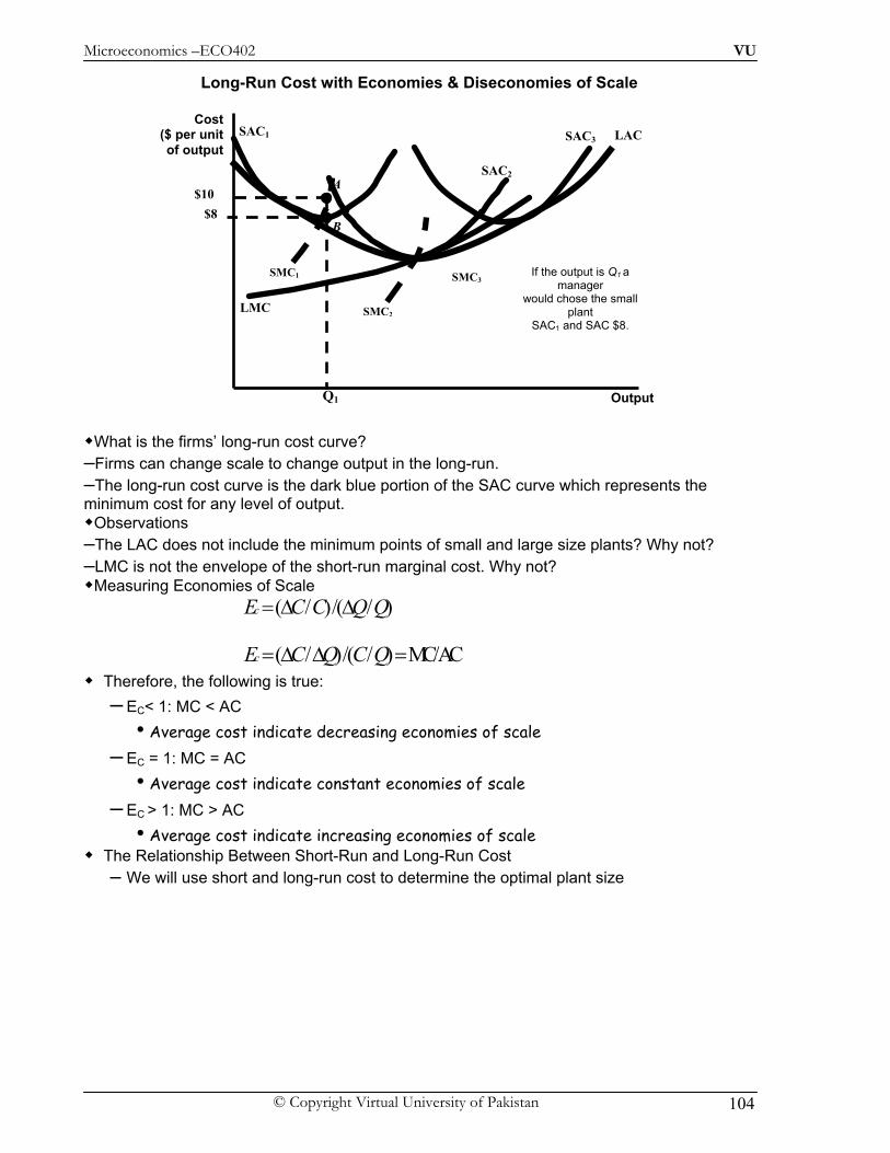
Microeconomics –ECO402 VU
© Copyright Virtual University of Pakistan 104
Long-Run Cost with Economies & Diseconomies of Scale
What is the firms’ long-run cost curve? –Firms can change scale to change output in the long-run. –The long-run cost curve is the dark blue portion of the SAC curve which represents the minimum cost for any level of output.
Observations –The LAC does not include the minimum points of small and large size plants? Why not? –LMC is not the envelope of the short-run marginal cost. Why not?
Measuring Economies of Scale ( / )/( / )cE C C Q Q= Δ Δ
( / )/( / ) MC/ACcE C Q C Q= Δ Δ =
Therefore, the following is true: – EC< 1: MC < AC
• Average cost indicate decreasing economies of scale – EC = 1: MC = AC
• Average cost indicate constant economies of scale – EC > 1: MC > AC
• Average cost indicate increasing economies of scale The Relationship Between Short-Run and Long-Run Cost
– We will use short and long-run cost to determine the optimal plant size
Output
Cost ($ per unit of output
SMC1
SAC1
SAC2
SMC2LMC
If the output is Q1 a manager
would chose the small plant
SAC1 and SAC $8.
$10
Q1
$8 B
A
LAC SAC3
SMC3
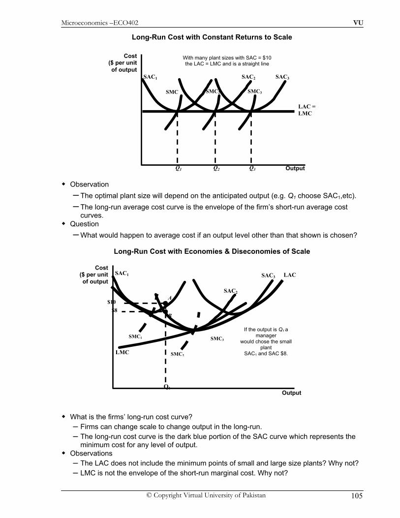
Microeconomics –ECO402 VU
© Copyright Virtual University of Pakistan 105
Long-Run Cost with Constant Returns to Scale
Observation – The optimal plant size will depend on the anticipated output (e.g. Q1 choose SAC1,etc). – The long-run average cost curve is the envelope of the firm’s short-run average cost
curves. Question
– What would happen to average cost if an output level other than that shown is chosen?
Long-Run Cost with Economies & Diseconomies of Scale
What is the firms’ long-run cost curve? – Firms can change scale to change output in the long-run. – The long-run cost curve is the dark blue portion of the SAC curve which represents the
minimum cost for any level of output. Observations
– The LAC does not include the minimum points of small and large size plants? Why not? – LMC is not the envelope of the short-run marginal cost. Why not?
LAC = LMC
With many plant sizes with SAC = $10 the LAC = LMC and is a straight line
Output
Cost ($ per unit of output
Q3
SAC3
SMC3
Q2
SAC2
SMC2
Q1
SAC1
SMC
Output
Cost ($ per unit of output
SMC1
SAC1
SAC2
SMC2LMC
LAC SAC3
SMC3
If the output is Q1 a manager
would chose the small plant
SAC1 and SAC $8.
$10
Q1
$8 B
A
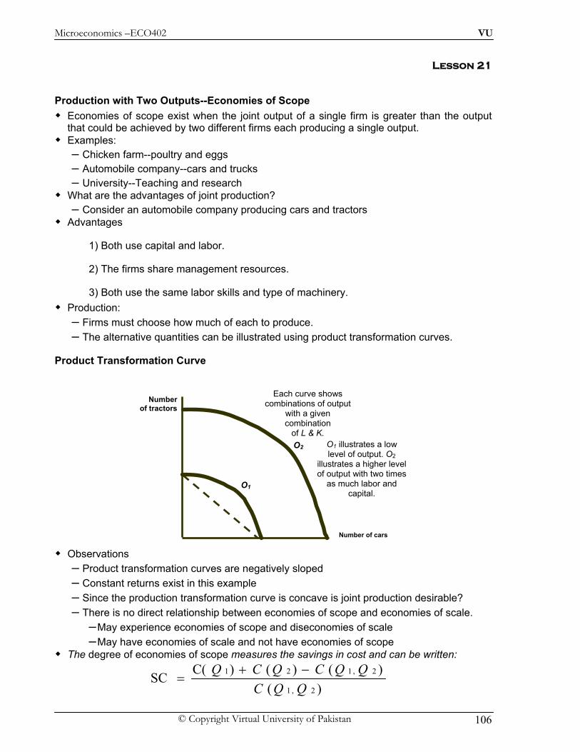
Microeconomics –ECO402 VU
© Copyright Virtual University of Pakistan 106
Lesson 21
Production with Two Outputs--Economies of Scope Economies of scope exist when the joint output of a single firm is greater than the output
that could be achieved by two different firms each producing a single output. Examples:
– Chicken farm--poultry and eggs – Automobile company--cars and trucks – University--Teaching and research
What are the advantages of joint production? – Consider an automobile company producing cars and tractors
Advantages
1) Both use capital and labor.
2) The firms share management resources.
3) Both use the same labor skills and type of machinery. Production:
– Firms must choose how much of each to produce. – The alternative quantities can be illustrated using product transformation curves.
Product Transformation Curve
Observations – Product transformation curves are negatively sloped – Constant returns exist in this example – Since the production transformation curve is concave is joint production desirable? – There is no direct relationship between economies of scope and economies of scale.
– May experience economies of scope and diseconomies of scale – May have economies of scale and not have economies of scope
The degree of economies of scope measures the savings in cost and can be written:
)()()()C( SC
2,1
2,121
QQCQQCQCQ −+
=
Number of cars
Number of tractors
O2 O1 illustrates a low level of output. O2
illustrates a higher level of output with two times
as much labor and capital.
O1
Each curve shows combinations of output
with a given combination
of L & K.

Microeconomics –ECO402 VU
© Copyright Virtual University of Pakistan 107
– C(Q1) is the cost of producing Q1
– C(Q2) is the cost of producing Q2
– C(Q1Q2) is the joint cost of producing both products Interpretation:
– If SC > 0 -- Economies of scope – If SC < 0 -- Diseconomies of scope
Issues – Truckload versus less than truck load – Direct versus indirect routing – Length of haul
Economies of Scope in the Trucking Industry Questions:
– Economies of Scope – Are large-scale, direct hauls cheaper and more profitable than individual hauls by
small trucks? – Are there cost advantages from operating both direct and indirect hauls?
Empirical Findings – An analysis of 105 trucking firms examined four distinct outputs.
– Short hauls with partial loads – Intermediate hauls with partial loads – Long hauls with partial loads – Hauls with total loads
– Results – SC = 1.576 for reasonably large firm – SC = 0.104 for very large firms
– Interpretation – Combining partial loads at an intermediate location lowers cost management
difficulties with very large firms.
Dynamic Changes in Costs--The Learning Curve The learning curve measures the impact of worker’s experience on the costs of
production. It describes the relationship between a firm’s cumulative output and amount of inputs
needed to produce a unit of output.
Cumulative number of machine lots produced
Hours of labor per machine lot
10 20 30 40 500
2
4
6
8
10

Microeconomics –ECO402 VU
© Copyright Virtual University of Pakistan 108
The horizontal axis measures the cumulative number of hours of machine tools the firm has
produced The vertical axis measures the number of hours of labor needed to produce each lot. The learning curve in the figure is based on the relationship:
L = A + BN-β
If N=1
– L equals A + B and this measures labor input to produce the first unit of output – If β = 0
– Labor input remains constant as the cumulative level of output increases, so there is no learning
If β > 0 and N increases – L approaches A, and A represent minimum labor input/unit of output after all learning
has taken place. – The larger β:
– The more important the learning effect.
Observations
1) New firms may experience a learning curve, not economies of scale.
2) Older firms have relatively small gains from learning.
Economies of Scale Versus Learning
Cumulative number of machine lots produced
Hours of labor per
machine lot
10 20 30 40 500
2
4
6
8
10
The chart shows a sharp drop in lots to a cumulative amount of
20, then small savings at higher levels.
Doubling cumulative output causesa 20% reduction in the difference between the input required and
minimum attainable input requirement
β = 0.31
Output
Cost ($ per unit of output)
AC1
B
Economies of Scale
A
AC2Learning C

Microeconomics –ECO402 VU
© Copyright Virtual University of Pakistan 109
Predicting the Labor Requirements of Producing a Given Output Cumulative Output Per-Unit Labor Requirement Total Labor (N) for each 10 units of Output (L) Requirement
10 1.00 10.0
20 .80 18.0 (10.0 + 8.0)
30 .70 25.0 (18.0 + 7.0)
40 .64 31.4 (25.0 + 6.4)
50 .60 37.4 (31.4 + 6.0)
60 .56 43.0 (37.4 + 5.6)
70 .53 48.3 (43.0 + 5.3)
80 and over .51 53.4 (48.3 + 5.1) The learning curve implies:
1) The labor requirement falls per unit.
2) Costs will be high at first and then will fall with learning.
3) After 8 years the labor requirement will be 0.51 and per unit cost will be half what it was in the first year of production?
Learning Curve in Practice Scenario
– A new firm enters the chemical processing industry. Do they:
1) Produce a low level of output and sell at a high price? 2) Produce a high level of output and sell at a low price?
How would the learning curve influence your decision? The Empirical Findings
– Study of 37 chemical products – Average cost fell 5.5% per year – For each doubling of plant size, average production costs fall by 11% – For each doubling of cumulative output, the average cost of production falls by 27%
Which is more important, the economies of scale or learning effects? Other Empirical Findings
– In the semi-conductor industry a study of seven generations of DRAM semiconductors from 1974-1992 found learning rates averaged 20%.
– In the aircraft industry the learning rates are as high as 40%. Applying Learning Curves
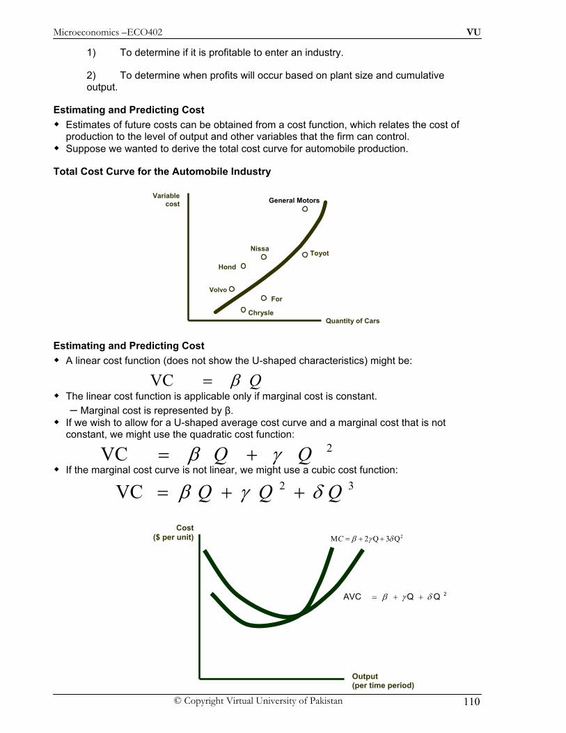
Microeconomics –ECO402 VU
© Copyright Virtual University of Pakistan 110
1) To determine if it is profitable to enter an industry.
2) To determine when profits will occur based on plant size and cumulative output.
Estimating and Predicting Cost Estimates of future costs can be obtained from a cost function, which relates the cost of
production to the level of output and other variables that the firm can control. Suppose we wanted to derive the total cost curve for automobile production.
Total Cost Curve for the Automobile Industry
Estimating and Predicting Cost A linear cost function (does not show the U-shaped characteristics) might be:
The linear cost function is applicable only if marginal cost is constant. – Marginal cost is represented by β.
If we wish to allow for a U-shaped average cost curve and a marginal cost that is not constant, we might use the quadratic cost function:
If the marginal cost curve is not linear, we might use a cubic cost function:
Qβ= VC
2 VC QQ γβ +=32 VC QQQ δγβ ++=
Quantity of Cars
Variable cost General Motors
Toyot
For
Chrysle
Volvo
Hond
Nissa
Output(per time period)
Cost ($ per unit)
2QQAVC δγβ ++=
2M 2 Q 3 QC β γ δ= + +
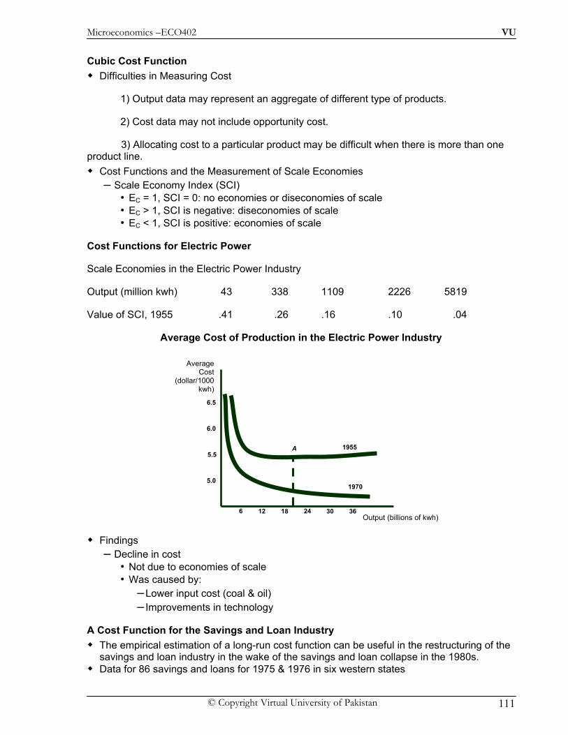
Microeconomics –ECO402 VU
© Copyright Virtual University of Pakistan 111
Cubic Cost Function Difficulties in Measuring Cost
1) Output data may represent an aggregate of different type of products.
2) Cost data may not include opportunity cost.
3) Allocating cost to a particular product may be difficult when there is more than one product line.
Cost Functions and the Measurement of Scale Economies – Scale Economy Index (SCI)
• EC = 1, SCI = 0: no economies or diseconomies of scale • EC > 1, SCI is negative: diseconomies of scale • EC < 1, SCI is positive: economies of scale
Cost Functions for Electric Power
Scale Economies in the Electric Power Industry
Output (million kwh) 43 338 1109 2226 5819
Value of SCI, 1955 .41 .26 .16 .10 .04
Average Cost of Production in the Electric Power Industry
Findings – Decline in cost
• Not due to economies of scale • Was caused by:
– Lower input cost (coal & oil) – Improvements in technology
A Cost Function for the Savings and Loan Industry The empirical estimation of a long-run cost function can be useful in the restructuring of the
savings and loan industry in the wake of the savings and loan collapse in the 1980s. Data for 86 savings and loans for 1975 & 1976 in six western states
Output (billions of kwh)
Average Cost
(dollar/1000 kwh)
5.0
5.5
6.0
6.5
6 12 18 24 30 36
1955
1970
A

Microeconomics –ECO402 VU
© Copyright Virtual University of Pakistan 112
– Q = total assets of each S&L – LAC = average operating expense – Q & TC are measured in hundreds of millions of dollars – Average operating cost are measured as a percentage of total assets.
A quadratic long-run average cost function was estimated for 1975:
Minimum long-run average cost reaches its point of minimum average total cost when total
assets of the savings and loan reach $574 million. Average operating expenses are 0.61% of total assets. Almost all of the savings and loans in the region being studied had substantially less than
$574 million in assets. Questions
1) What are the implications of the analysis for expansion and mergers?
2) What are the limitations of using these results?
20.0536Q 0.6153Q - 2.38 LAC +=
Microeconomics –ECO402 VU
© Copyright Virtual University of Pakistan 113
Lesson 22
Perfectly Competitive Markets Characteristics of Perfectly Competitive Markets
1) Price taking
2) Product homogeneity
3) Free entry and exit Price Taking
– The individual firm sells a very small share of the total market output and, therefore, cannot influence market price.
– The individual consumer buys too small a share of industry output to have any impact on market price.
Product Homogeneity – The products of all firms are perfect substitutes. – Examples
• Agricultural products, oil, copper, iron, lumber Free Entry and Exit
– Buyers can easily switch from one supplier to another. – Suppliers can easily enter or exit a market.
Discussion Questions – What are some barriers to entry and exit? – Are all markets competitive? – When is a market highly competitive?
Do firms maximize profits? – Possibility of other objectives
• Revenue maximization • Dividend maximization • Short-run profit maximization
– Implications of non-profit objective • Over the long-run investors would not support the company • Without profits, survival unlikely
– Long-run profit maximization is valid and does not exclude the possibility of altruistic behavior.
Marginal Revenue, Marginal Cost & Profit Maximization Determining the profit maximizing level of output
– Profit (π ) = Total Revenue - Total Cost – Total Revenue (R) = Pq – Total Cost (C) = Cq – Therefore:
( ) ( ) ( )q R q C qπ = −

Microeconomics –ECO402 VU
© Copyright Virtual University of Pakistan 114
Profit Maximization in the Short Run
Marginal Revenue, Marginal Cost & Profit Maximization Marginal revenue is the additional revenue from producing one more unit of output. Marginal cost is the additional cost from producing one more unit of output.
0
Cost, Revenue,
Profit ($s per
year)
Output (units per year)
R(q) Total Revenue
Slope of R(q) = MR
0
Cost, Revenue,
Profit $ (per year)
Output (units per year)
C(q)
Total Cost
Slope of C(q) = MC
Why is cost positive when q is zero?
0
Cost, Revenue,
Profit ($s per year)
Output (units per year)
R(q)
C(q)
A
B
q0 q*
π (q)
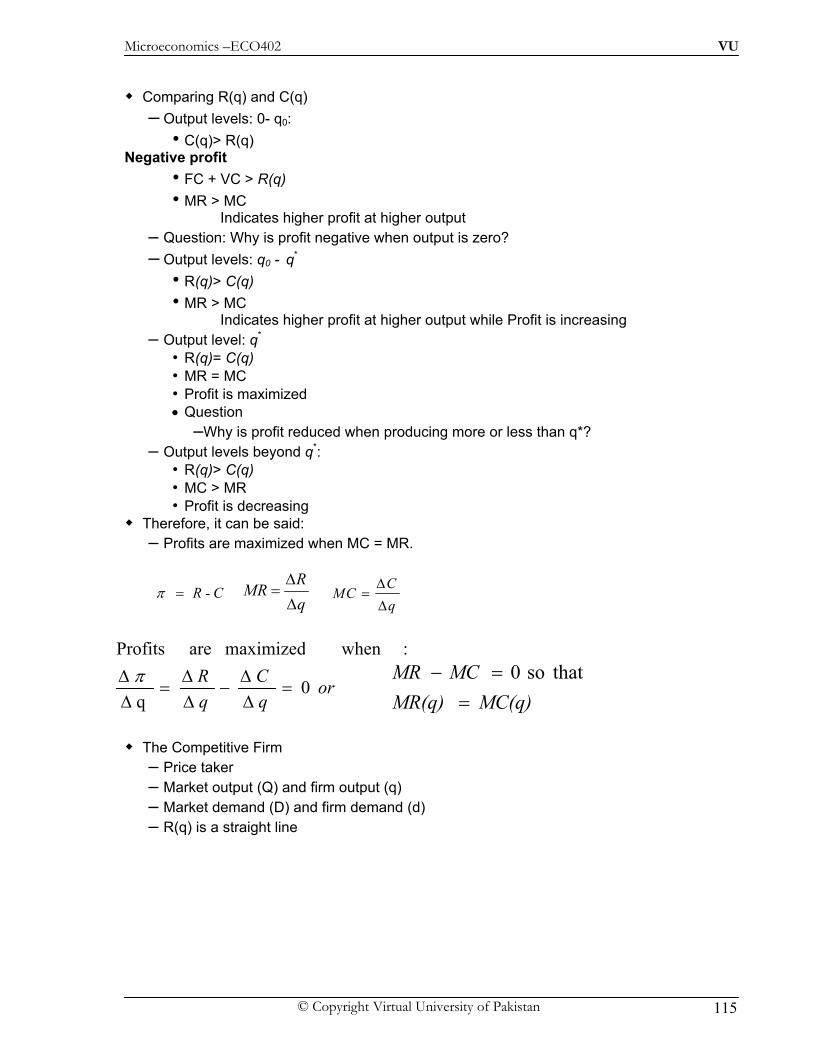
Microeconomics –ECO402 VU
© Copyright Virtual University of Pakistan 115
Comparing R(q) and C(q)
– Output levels: 0- q0: • C(q)> R(q)
Negative profit • FC + VC > R(q) • MR > MC
Indicates higher profit at higher output – Question: Why is profit negative when output is zero? – Output levels: q0 - q*
• R(q)> C(q) • MR > MC
Indicates higher profit at higher output while Profit is increasing – Output level: q*
• R(q)= C(q) • MR = MC • Profit is maximized • Question
–Why is profit reduced when producing more or less than q*? – Output levels beyond q*:
• R(q)> C(q) • MC > MR • Profit is decreasing
Therefore, it can be said: – Profits are maximized when MC = MR.
R - Cπ = RMR
qΔ
=Δ
CMC
qΔ
=Δ
The Competitive Firm – Price taker – Market output (Q) and firm output (q) – Market demand (D) and firm demand (d) – R(q) is a straight line
orqC
qR 0
q
:whenmaximized are Profits
=ΔΔ
−ΔΔ
=ΔΔ π
MC(q)MR(q)MCMR=
=− thatso0
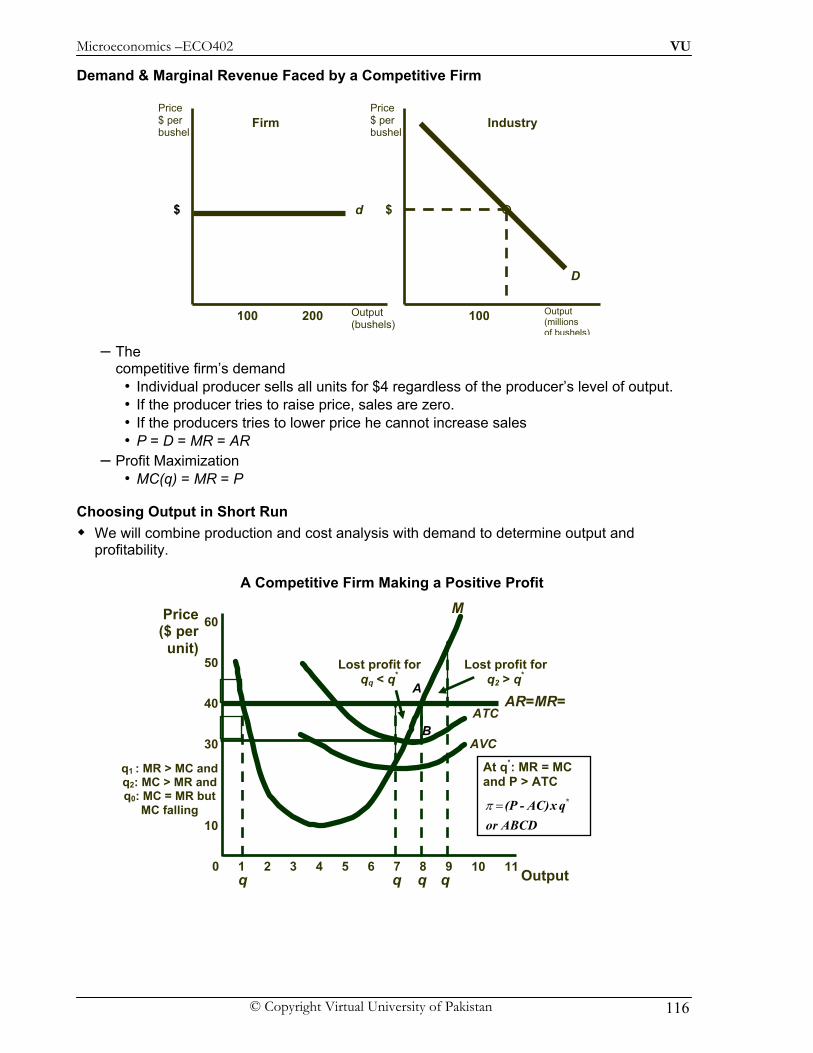
Microeconomics –ECO402 VU
© Copyright Virtual University of Pakistan 116
Demand & Marginal Revenue Faced by a Competitive Firm
– The competitive firm’s demand
• Individual producer sells all units for $4 regardless of the producer’s level of output. • If the producer tries to raise price, sales are zero. • If the producers tries to lower price he cannot increase sales • P = D = MR = AR
– Profit Maximization • MC(q) = MR = P
Choosing Output in Short Run We will combine production and cost analysis with demand to determine output and
profitability.
A Competitive Firm Making a Positive Profit
Output (bushels)
Price $ per bushel
Price $ per bushel
Output (millions of bushels)
d$
100 200 100
Firm Industry
D
$
q
Lost profit forqq < q*
Lost profit forq2 > q*
q q
AR=MR=
10
30
40
Price ($ per
unit)
0 1 2 3 4 5 6 7 8 9 10 11
50
60 M
AVC
ATC
Outputq*
At q*: MR = MC and P > ATC
ABCDorqx AC) -(P *= π
D A
BC
q1 : MR > MC and q2: MC > MR and q0: MC = MR but
MC falling
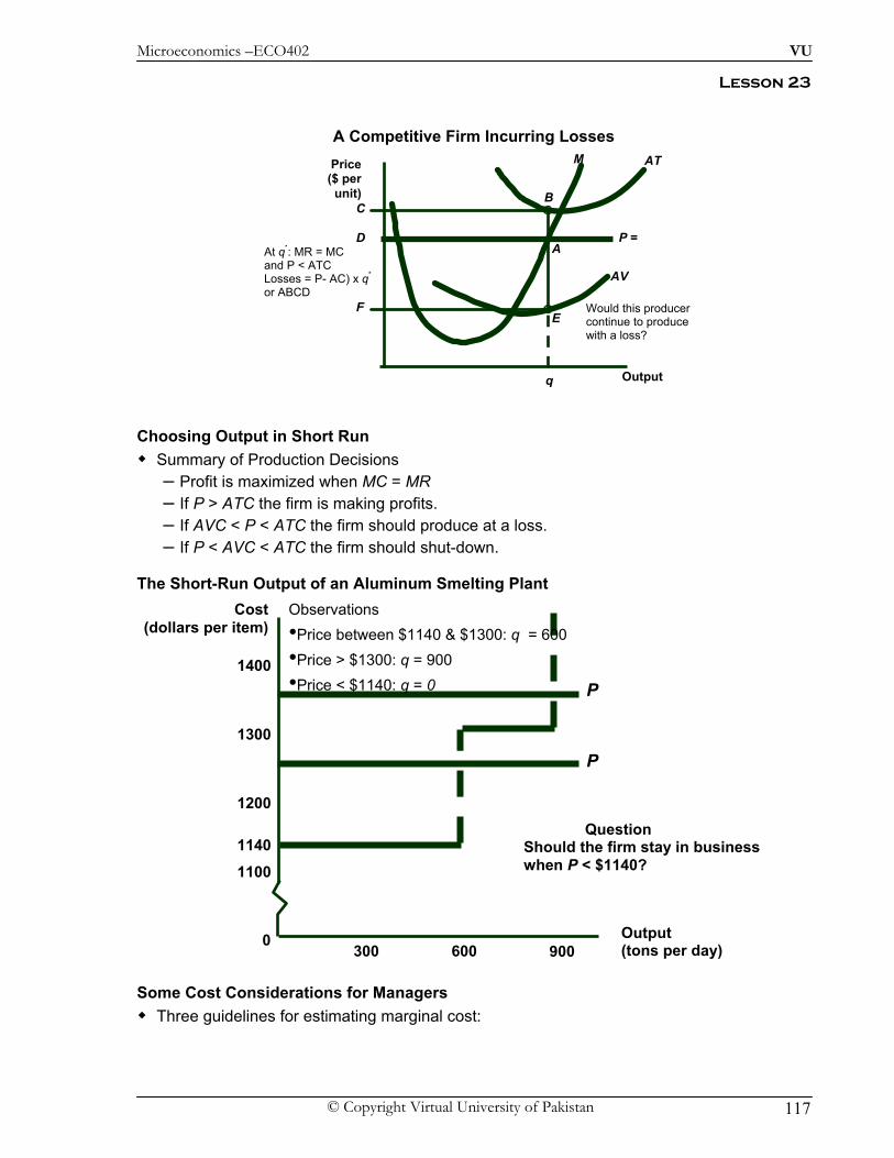
Microeconomics –ECO402 VU
© Copyright Virtual University of Pakistan 117
Lesson 23
A Competitive Firm Incurring Losses
Choosing Output in Short Run Summary of Production Decisions
– Profit is maximized when MC = MR – If P > ATC the firm is making profits. – If AVC < P < ATC the firm should produce at a loss. – If P < AVC < ATC the firm should shut-down.
The Short-Run Output of an Aluminum Smelting Plant
Some Cost Considerations for Managers Three guidelines for estimating marginal cost:
Output (tons per day)
Cost(dollars per item)
300 600 9000
1100
1200
1300
1400
1140
P
P
Observations •Price between $1140 & $1300: q = 600 •Price > $1300: q = 900 •Price < $1140: q = 0
Question Should the firm stay in business when P < $1140?
Would this producer continue to produce with a loss?
Price($ per
unit)
Output
AV
ATM
q*
P =
B
F
C
A
E
DAt q*: MR = MC and P < ATC Losses = P- AC) x q* or ABCD

Microeconomics –ECO402 VU
© Copyright Virtual University of Pakistan 118
1) Average variable cost should not be used as a substitute for marginal cost.
2) A single item on a firm’s accounting ledger may have two components, only one of which involves marginal cost.
3) All opportunity cost should be included in determining marginal cost.
A Competitive Firm’s Short-Run Supply Curve
Observations: – P = MR – MR = MC – P = MC
Supply is the amount of output for every possible price. Therefore: – If P = P1, then q = q1
– If P = P2, then q = q2
Observations:
– Supply is upward sloping due to diminishing returns. – Higher price compensates the firm for higher cost of additional output and increases
total profit because it applies to all units. Firm’s Response to an Input Price Change
Price ($ per
unit)
Output
MC
AVC
ATC
P = AVC What happens
if P < AVC?
P2
q2
P1
q1
The firm chooses the output level where MR = MC, as long as the firm is able to cover its variable cost of
production.
Price ($ per
unit) MC
Output
AVC
ATC
P = AVC
P1
P2
q1 q2
S = MC above AVC
Shut-down
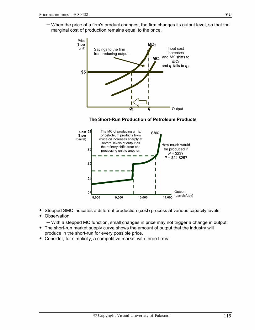
Microeconomics –ECO402 VU
© Copyright Virtual University of Pakistan 119
– When the price of a firm’s product changes, the firm changes its output level, so that the marginal cost of production remains equal to the price.
The Short-Run Production of Petroleum Products
Stepped SMC indicates a different production (cost) process at various capacity levels. Observation:
– With a stepped MC function, small changes in price may not trigger a change in output. The short-run market supply curve shows the amount of output that the industry will
produce in the short-run for every possible price. Consider, for simplicity, a competitive market with three firms:
$5
MC2
q2
Input cost increases
and MC shifts to MC2
and q falls to q2.
MC1
q
Price ($ per
unit)
Output
Savings to the firm from reducing output
Cost ($ per
barrel)
Output (barrels/day) 8,000 9,000 10,000 11,000
23
24
25
26
27 SMC
How much would be produced if
P = $23? P = $24-$25?
The MC of producing a mix of petroleum products from
crude oil increases sharply at several levels of output as the refinery shifts from one processing unit to another.
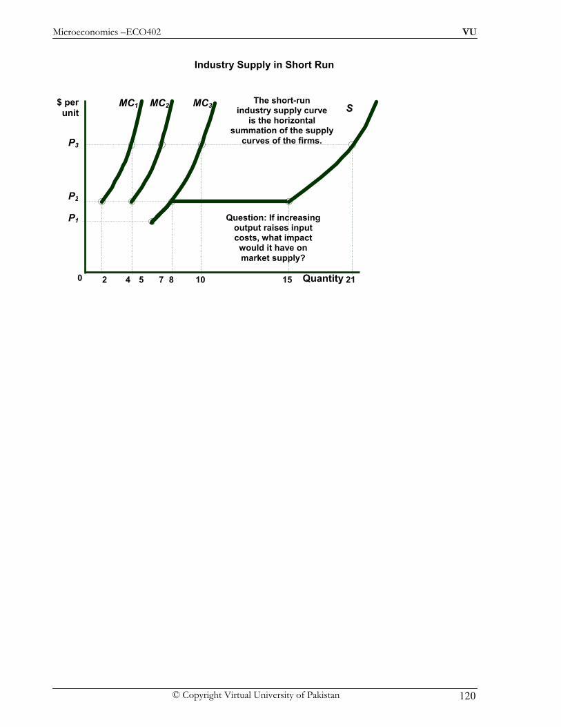
Microeconomics –ECO402 VU
© Copyright Virtual University of Pakistan 120
Industry Supply in Short Run
MC3 $ per unit
0 2 4 8 10 5 7 15 21
MC1 SS The short-run
industry supply curve is the horizontal
summation of the supply curves of the firms.
Quantity
MC2
P1
P3
P2
Question: If increasingoutput raises input costs, what impact would it have on market supply?

Microeconomics –ECO402 VU
© Copyright Virtual University of Pakistan 121
Lesson 24
Elasticity of Market Supply
• Perfectly inelastic short-run supply arises when the industry’s plant and equipment are so
fully utilized that new plants must be built to achieve greater output. • Perfectly elastic short-run supply arises when marginal costs are constant.
The World Copper Industry (1999)
Annual Production Marginal Cost Country (thousand metric tons) (dollars/pound) Australia 600 0.65 Canada 710 0.75 Chile 3660 0.50 Indonesia 750 0.55 Peru 450 0.70 Poland 420 0.80 Russia 450 0.50 United States 1850 0.55
The Short-Run World Supply of Copper
Producer Surplus in the Short Run – Firms earn a surplus on all but the last unit of output. – The producer surplus is the sum over all units produced of the difference between the
market price of the good and the marginal cost of production.
)//()/( PPQQE s ΔΔ=
Production (thousand metric tons)
Price ($ per pound)
0 2000 4000 6000 8000 10000 0.40
0.50
0.60
0.70
0.80
0.90
MCC,MCMCJ,MC
MCMCP,MCU
MCC
MCP

Microeconomics –ECO402 VU
© Copyright Virtual University of Pakistan 122
Producer Surplus in the Short-Run Producer Surplus PS R - VC= = P ro fit - R - V C - F Cπ=
Observation – Short-run with positive fixed cost
P S π>
Producer Surplus for a Market
Choosing Output in Long Run In the long run, a firm can alter all its inputs, including the size of the plant. We assume free entry and free exit.
MC
Price ($ per
unit of output)
Output00
PP
qq**
At q* MC = MR. Between 0 and q ,
MR > MC for all units.
AA
DD
BB
CC
Producer Surplus
Alternatively, VC is the sum of MC or ODCq* . R is P x q* or OABq*. Producer surplus = R - VC or ABCD.
AVC
D
Price ($ per
unit of output)
Output
S
P*
Q*
Producer
Market producer surplus is the difference between P*
and S from 0 to Q*.
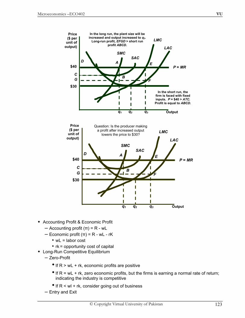
Microeconomics –ECO402 VU
© Copyright Virtual University of Pakistan 123
Accounting Profit & Economic Profit – Accounting profit (π) = R - wL – Economic profit (π) = R - wL - rK
• wL = labor cost • rk = opportunity cost of capital
Long-Run Competitive Equilibrium – Zero-Profit
• If R > wL + rk, economic profits are positive
• If R = wL + rk, zero economic profits, but the firms is earning a normal rate of return; indicating the industry is competitive
• If R < wl + rk, consider going out of business – Entry and Exit
q1
A
BC
D
In the short run, the firm is faced with fixed inputs. P = $40 > ATC. Profit is equal to ABCD.
Price ($ per
unit of output)
Output
P = MR $40
SACSMC
In the long run, the plant size will be increased and output increased to q3.
Long-run profit, EFGD > short run profit ABCD.
q3 q2
G F$30
LAC
E
LMC
q1
A
BC
D
Price ($ per
unit of output)
Output
P = MR $40
SACSMC
Question: Is the producer makinga profit after increased output
lowers the price to $30?
q3 q2
G F$30
LAC
E
LMC

Microeconomics –ECO402 VU
© Copyright Virtual University of Pakistan 124
• The long-run response to short-run profits is to increase output and profits.
• Profits will attract other producers.
• More producers increase industry supply which lowers the market price.
Long-Run Competitive Equilibrium
Long-Run Competitive Equilibrium
1) MC = MR
2) P = LAC
• No incentive to leave or enter
• Profit = 0
3) Equilibrium Market Price Questions
1) Explain the market adjustment when P < LAC and firms have identical costs.
2) Explain the market adjustment when firms have different costs.
3) What is the opportunity cost of land? Economic Rent
– Economic rent is the difference between what firms are willing to pay for an input less the minimum amount necessary to obtain it.
An Example – Two firms A & B – Both own their land – A is located on a river which lowers A’s shipping cost by $10,000 compared to B –
S
Output Output
$ per unit ofoutput
$ per unit of output
$40 LAC
LMC
D
SP
Qq2
Firm Industry
$30
Q2
P2
•Profit attracts firms •Supply increases until profit = 0
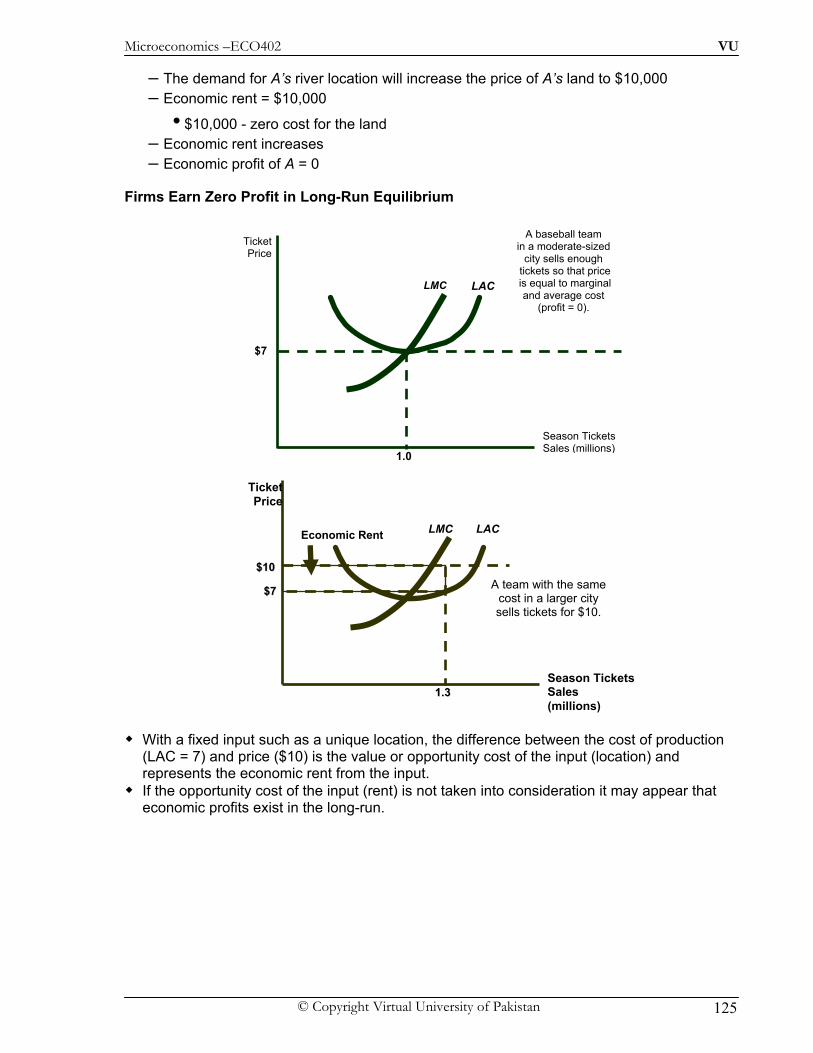
Microeconomics –ECO402 VU
© Copyright Virtual University of Pakistan 125
– The demand for A’s river location will increase the price of A’s land to $10,000 – Economic rent = $10,000
• $10,000 - zero cost for the land – Economic rent increases – Economic profit of A = 0
Firms Earn Zero Profit in Long-Run Equilibrium
With a fixed input such as a unique location, the difference between the cost of production (LAC = 7) and price ($10) is the value or opportunity cost of the input (location) and represents the economic rent from the input.
If the opportunity cost of the input (rent) is not taken into consideration it may appear that economic profits exist in the long-run.
Ticket Price
Season Tickets Sales (millions)
LAC
$7
1.0
A baseball team in a moderate-sized
city sells enough tickets so that price is equal to marginal
and average cost (profit = 0).
LMC
11..33
$$1100
Economic Rent
Ticket Price
$$77
LAC
A team with the same cost in a larger city sells tickets for $10.
Season Tickets Sales (millions)
LMC

Microeconomics –ECO402 VU
© Copyright Virtual University of Pakistan 126
Lesson 26
The Industry’s Long-Run Supply Curve Long-Run Elasticity of Supply
1) Constant-cost industry
• Long-run supply is horizontal
• Small increase in price will induce an extremely large output increase
• Long-run supply elasticity is infinitely large
• Inputs would be readily available
2) Increasing-cost industry
• Long-run supply is upward-sloping and elasticity is positive
• The slope (elasticity) will depend on the rate of increase in input cost
• Long-run elasticity will generally be greater than short-run elasticity of supply
The Industry’s Long-Run Supply Curve Question:
– Describe the long-run elasticity of supply in a decreasing -cost industry.
The Long-Run Supply of Housing Scenario 1: Owner-occupied housing
– Suburban or rural areas – National market for inputs
Questions – Is this an increasing or a constant-cost industry? – What would you predict about the elasticity of supply?
Scenario 2: Rental property – Urban location – High-rise construction cost
Questions – Is this an increasing or a constant-cost industry? – What would you predict about the elasticity of supply?
The Industry’s Long-Run Supply Curve The Effects of a Tax
– In an earlier chapter we studied how firms respond to taxes on an input. – Now, we will consider how a firm responds to a tax on its output.

Microeconomics –ECO402 VU
© Copyright Virtual University of Pakistan 127
Effect of an Output Tax on a Competitive Firm’s Output
Effect of an Output Tax on Industry Output
Evaluating the Gains & Losses from Government Policies:
Consumer & Producer Surplus Review
– Consumer surplus is the total benefit or value that consumers receive beyond what they pay for the good.
– Producer surplus is the total benefit or revenue that producers receive beyond what it cost to produce a good.
Price ($ per
unit of output)
Output
AVC
MC
P
q
The firm will reduce output to
the point at which the marginal cost
plus the tax equals the price.
q
tt
MC2 = MC1 + tax
AVC
An output tax raises the firm’s
marginal cost by the amount of the tax.
Price ($ per
unit of output)
Output
D
P
S
Q
P
Q
S2 = S1 + t
tTax shifts S1 to S2 and output falls to Q2. Price
increases to P2.
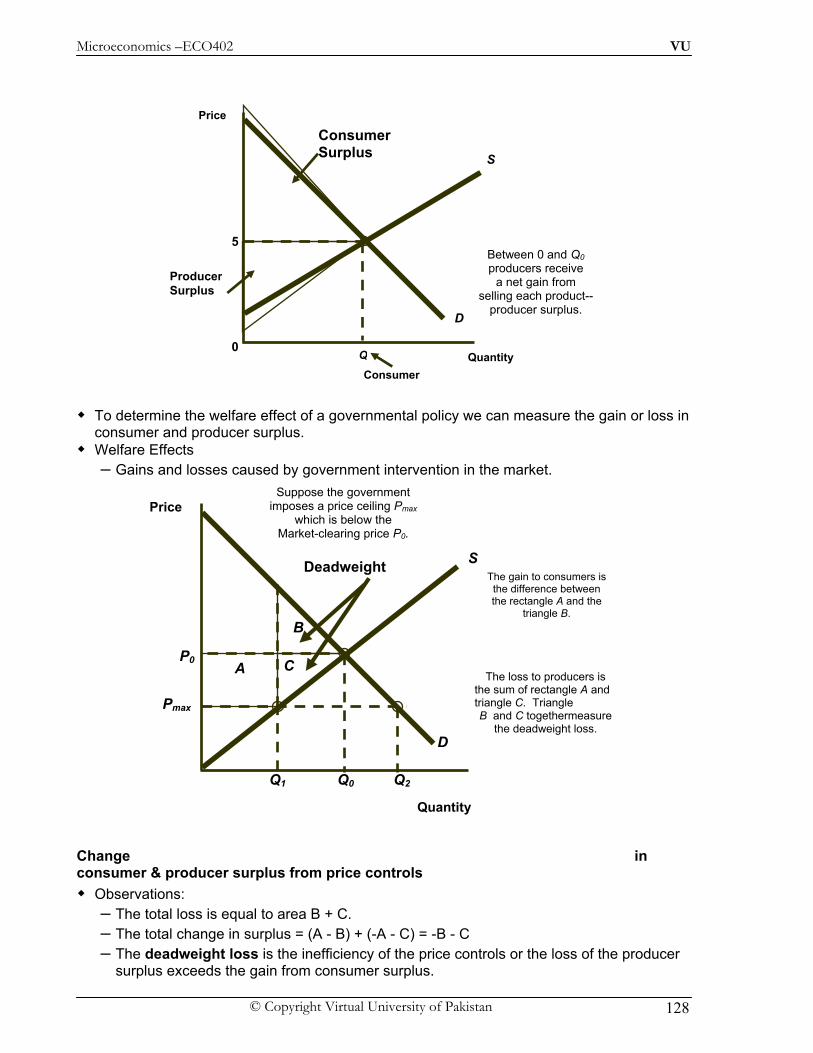
Microeconomics –ECO402 VU
© Copyright Virtual University of Pakistan 128
To determine the welfare effect of a governmental policy we can measure the gain or loss in consumer and producer surplus.
Welfare Effects – Gains and losses caused by government intervention in the market.
Change in consumer & producer surplus from price controls
Observations: – The total loss is equal to area B + C. – The total change in surplus = (A - B) + (-A - C) = -B - C – The deadweight loss is the inefficiency of the price controls or the loss of the producer
surplus exceeds the gain from consumer surplus.
Producer Surplus
Between 0 and Q0 producers receive
a net gain from selling each product--
producer surplus.
Consumer Surplus
Quantity0
Price
S
D
5
Q
Consumer
The loss to producers is the sum of rectangle A and triangle C. Triangle B and C togethermeasure
the deadweight loss.
B
A C
The gain to consumers is the difference between the rectangle A and the
triangle B.
Deadweight
Quantity
Price
S
D
P0
Q0
Pmax
Q1 Q2
Suppose the government imposes a price ceiling Pmax
which is below the Market-clearing price P0.
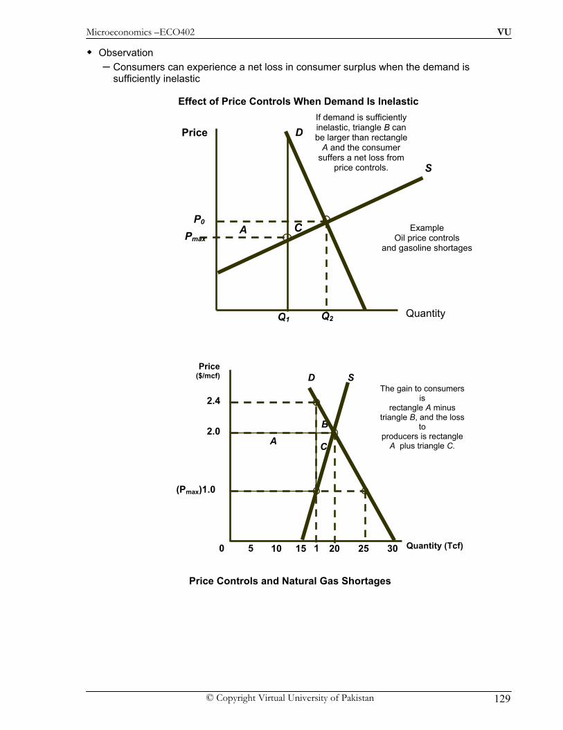
Microeconomics –ECO402 VU
© Copyright Virtual University of Pakistan 129
Observation – Consumers can experience a net loss in consumer surplus when the demand is
sufficiently inelastic
Effect of Price Controls When Demand Is Inelastic
Price Controls and Natural Gas Shortages
APmax C
Q1
If demand is sufficiently inelastic, triangle B can be larger than rectangle
A and the consumer suffers a net loss from
price controls.
Example Oil price controls
and gasoline shortages
S
D
Quantity
Price
P0
Q2
B
A
2.4
C
The gain to consumers is
rectangle A minus triangle B, and the loss
to producers is rectangle
A plus triangle C.
SD
2.0
Quantity (Tcf)0
Price ($/mcf)
5 10 15 20 25 30 1
(Pmax)1.0
Microeconomics –ECO402 VU
© Copyright Virtual University of Pakistan 130
The Efficiency of a Competitive Market When do competitive markets generate an inefficient allocation of resources or market
failure?
1) Externalities
• Costs or benefits that do not show up as part of the market price (e.g. pollution)
2) Lack of Information
• Imperfect information prevents consumers from making utility-maximizing decisions. Government intervention in these markets can increase efficiency. Government intervention without a market failure creates inefficiency or deadweight loss.

Microeconomics –ECO402 VU
© Copyright Virtual University of Pakistan 131
Lesson 27
Welfare loss if price is held below market-clearing level
Welfare loss if price is held above market-clearing level
P
Q
A
B
C
When price is regulated to be no higher than P1, the
deadweight loss given by triangles B and C results.
Quantity
Price
S
D
P
Q
Quantity
Price
P
Q
A B
C
Q
What would the deadweight loss be if QS = Q2?
When price is regulated to be no
lower than P2 only Q3 will be demanded. The
deadweight loss is given by triangles B and C S
D
P
Q
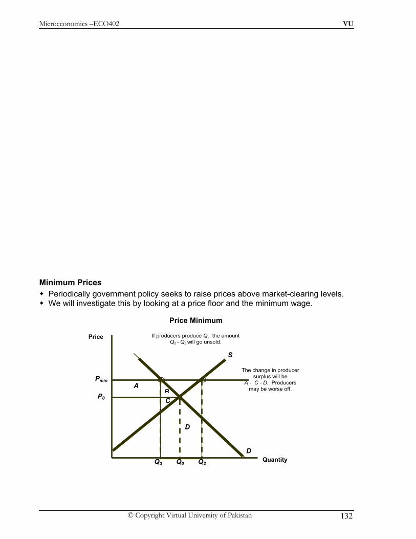
Microeconomics –ECO402 VU
© Copyright Virtual University of Pakistan 132
Minimum Prices Periodically government policy seeks to raise prices above market-clearing levels. We will investigate this by looking at a price floor and the minimum wage.
Price Minimum
BA
The change in producer surplus will be
A - C - D. Producers may be worse off.
C
D
Quantity
Price
S
D
P0
Q0
Pmin
Q3 Q2
If producers produce Q2, the amount Q2 - Q3 will go unsold.
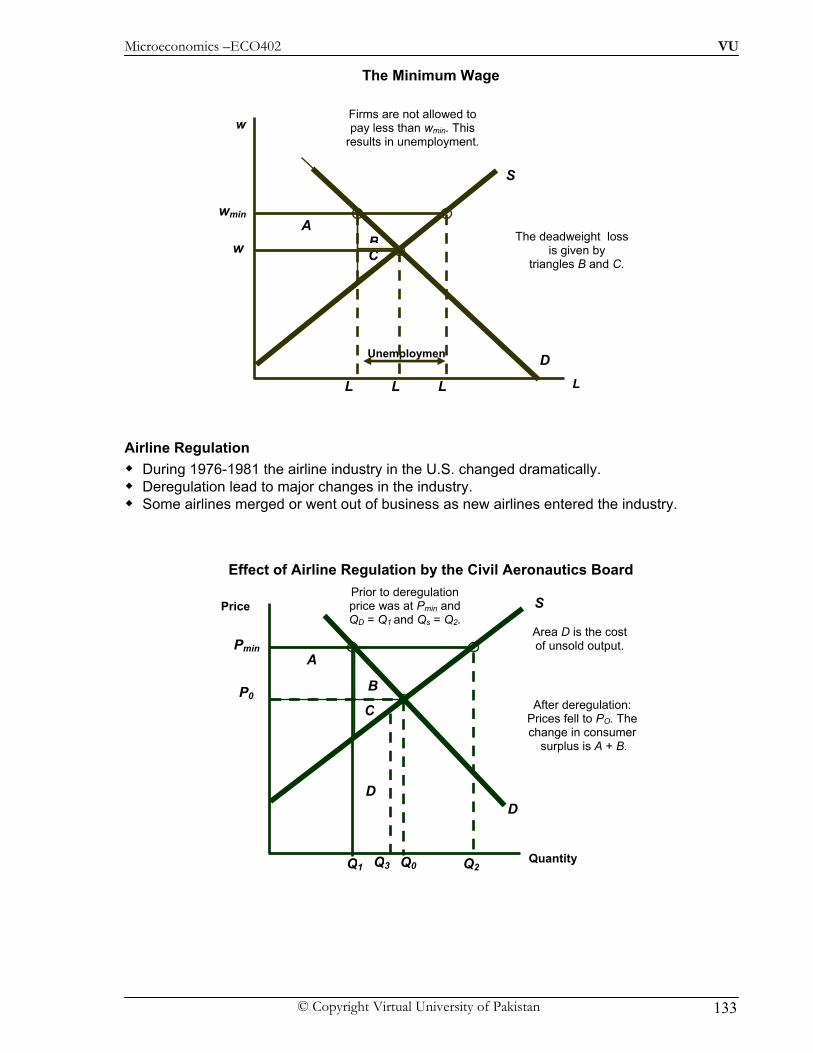
Microeconomics –ECO402 VU
© Copyright Virtual University of Pakistan 133
The Minimum Wage
Airline Regulation During 1976-1981 the airline industry in the U.S. changed dramatically. Deregulation lead to major changes in the industry. Some airlines merged or went out of business as new airlines entered the industry.
Effect of Airline Regulation by the Civil Aeronautics Board
B The deadweight loss is given by
triangles B and C. C
A wmin
L L
Unemploymen
Firms are not allowed to pay less than wmin. This
results in unemployment.
S
D
w
L L
w
B
A
C After deregulation: Prices fell to PO. The change in consumer
surplus is A + B.
Q3
D
Area D is the cost of unsold output.
Quantity
Price S
D
P0
Q0 Q1
Pmin
Q2
Prior to deregulation price was at Pmin and QD = Q1 and Qs = Q2.

Microeconomics –ECO402 VU
© Copyright Virtual University of Pakistan 134
Lesson 28
Price Supports
Question: – Is there a more efficient way to increase farmer’s income by A + B + D?
Price Supports and Production Quotas Production Quotas
– The government can also cause the price of a good to rise by reducing supply. What is the impact of controlling entry into the taxicab market?
BDA
To maintain a price Ps the government buys
quantity Qg . The change in consumer surplus = -A - B, and the change in producer
surplus is A + B + D
D +
Q
Quantity
Price S
D
P
Q
P
D +
Q
B A
Quantity
Price S
D
P0
Q0
Ps
Q2Q1
The cost to the government is the speckled rectangle
Ps(Q2-Q1)
D
Total Welfare
Loss
Total welfare loss D-(Q2-Q1)ps

Microeconomics –ECO402 VU
© Copyright Virtual University of Pakistan 135
Supply Restrictions
∆PS =A - C + B + C + D =A + B + D.
The change in consumer and producer surplus is the same as with price supports. ∆welfare = -A - B + A + B + D - B - C - D = -B - C.
Questions:
– How could the government reduce the cost and still subsidize the farmer? – Which is more costly: supports or acreage limitations?
•CS reduced by A + B
•Change in PS = A - C C
D
Quantity
Price
D
P
Q
SPS
S’
Q
• Supply restricted to Q1
• Supply shifts to S’ @ Q1
B
A
C
D
Quantity
Price
D
P
Q
S
P
S
Q
•Ps is maintained with and incentive
•Cost to government = B + C + D
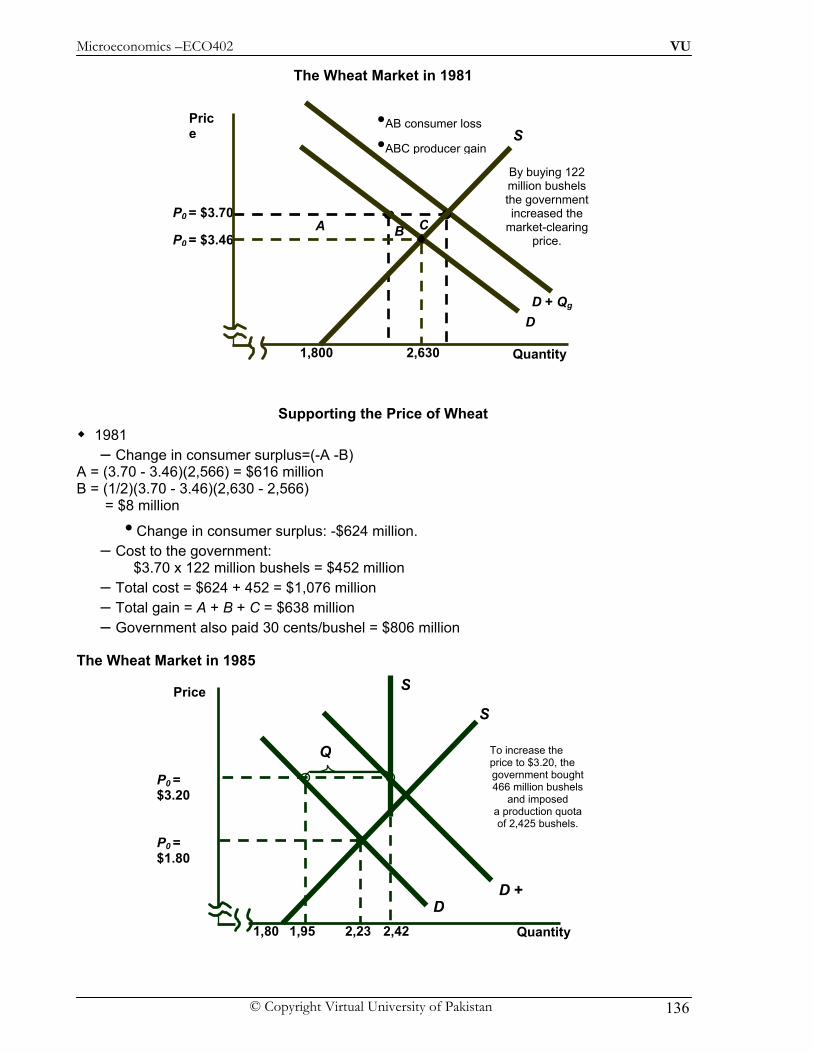
Microeconomics –ECO402 VU
© Copyright Virtual University of Pakistan 136
The Wheat Market in 1981
Supporting the Price of Wheat 1981
– Change in consumer surplus=(-A -B) A = (3.70 - 3.46)(2,566) = $616 million B = (1/2)(3.70 - 3.46)(2,630 - 2,566) = $8 million
• Change in consumer surplus: -$624 million. – Cost to the government:
$3.70 x 122 million bushels = $452 million – Total cost = $624 + 452 = $1,076 million – Total gain = A + B + C = $638 million – Government also paid 30 cents/bushel = $806 million
The Wheat Market in 1985
D + Qg
By buying 122 million bushels the government increased the
market-clearing price.
P0 = $3.70
2,56 2,68
A B C
Q
•AB consumer loss
•ABC producer gainS
D
P0 = $3.46
2,6301,800 Quantity
Price
Quantity
Price
1,80
S
D
P0 = $1.80
2,23
To increase the price to $3.20, the government bought 466 million bushels
and imposed a production quota of 2,425 bushels.
D +
S
P0 = $3.20
1,95 2,42
Q
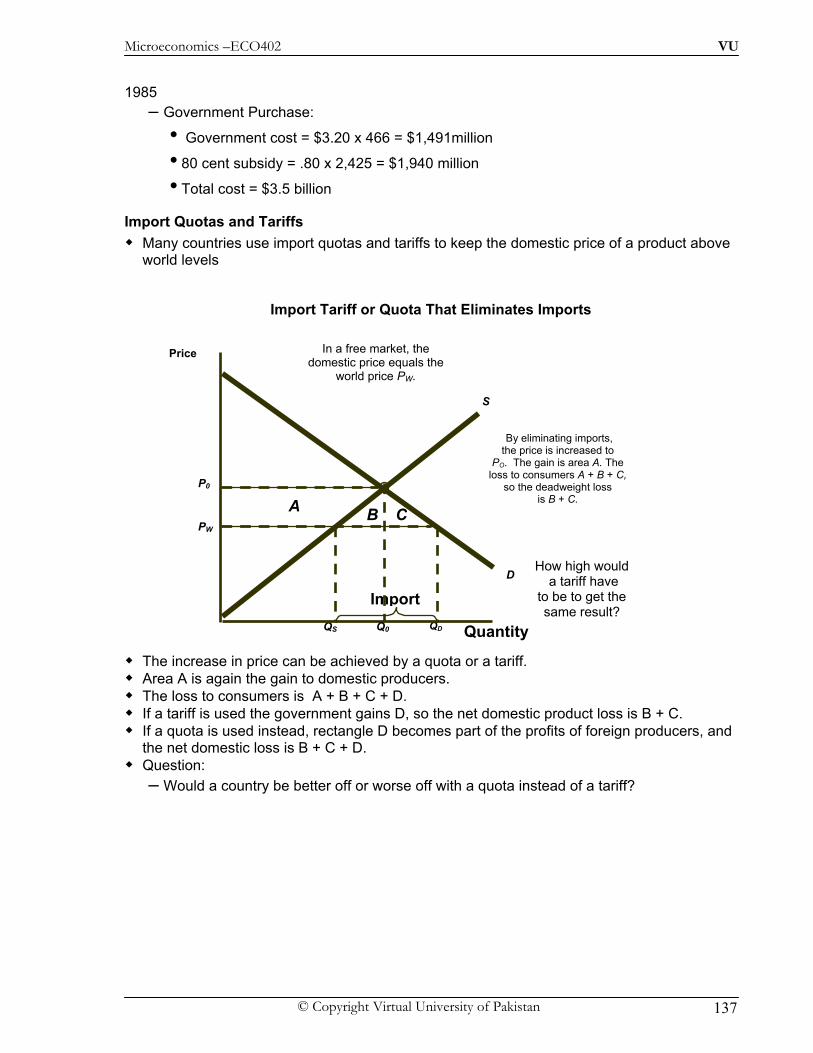
Microeconomics –ECO402 VU
© Copyright Virtual University of Pakistan 137
1985
– Government Purchase:
• Government cost = $3.20 x 466 = $1,491million
• 80 cent subsidy = .80 x 2,425 = $1,940 million
• Total cost = $3.5 billion
Import Quotas and Tariffs Many countries use import quotas and tariffs to keep the domestic price of a product above
world levels
Import Tariff or Quota That Eliminates Imports
The increase in price can be achieved by a quota or a tariff. Area A is again the gain to domestic producers. The loss to consumers is A + B + C + D. If a tariff is used the government gains D, so the net domestic product loss is B + C. If a quota is used instead, rectangle D becomes part of the profits of foreign producers, and
the net domestic loss is B + C + D. Question:
– Would a country be better off or worse off with a quota instead of a tariff?
QS QD
PW
Import
A B C
By eliminating imports, the price is increased to
PO. The gain is area A. The loss to consumers A + B + C,
so the deadweight loss is B + C.
Quantity
Price
How high would a tariff have
to be to get the same result?
D
P0
Q0
S
In a free market, the domestic price equals the
world price PW.

Microeconomics –ECO402 VU
© Copyright Virtual University of Pakistan 138
– Lesson 29
The Sugar Quota The world price of sugar has been as low as 4 cents per pound, while in the U.S. the price
has been 20-25 cents per pound. The Impact of a Restricted Market (1997)
– U.S. production = 15.6 billion pounds – U.S. consumption = 21.1 billion pounds – U.S. price = 22 cents/pound – World price = 11 cents/pound
Sugar Quota in 1997
C
D
B
QS = 4.0 Q’S = 15.6 Q’d = 21.1
Qd = 24.2
A
Quantity (billions of pounds)
Price (cents/lb.)
SUS DUS
5 10 15 20 250
4
8
11
16
20
PW = 11
PUS = 21.9
30
Rectangle D was the gain to foreign producers
who obtained quota allotments, or $600 million.
Triangles B and C representthe deadweight loss of
$800 million.
C
D
B
QS = 4.0 Q’S = 15.6 Q’d = 21.1
Qd = 24.2
A The cost of the quotas
to consumers was A + B + C + D, or $2.4b. The gain to producers
was area A, or $1b.
Quantity (billions of pounds)
Price (cents/lb.)
SUS DUS
5 10 15 20 250
4
8
11
16
20
PW = 11
PUS = 21.9
30
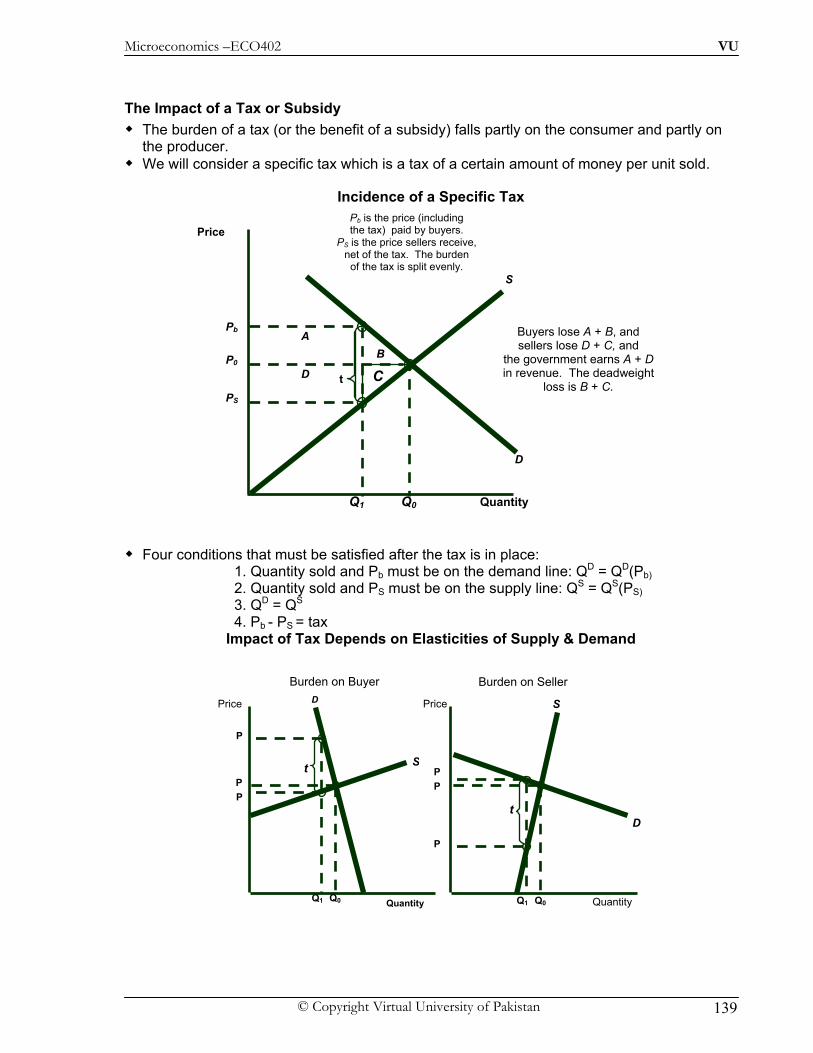
Microeconomics –ECO402 VU
© Copyright Virtual University of Pakistan 139
The Impact of a Tax or Subsidy The burden of a tax (or the benefit of a subsidy) falls partly on the consumer and partly on
the producer. We will consider a specific tax which is a tax of a certain amount of money per unit sold.
Incidence of a Specific Tax
Four conditions that must be satisfied after the tax is in place: 1. Quantity sold and Pb must be on the demand line: QD = QD(Pb) 2. Quantity sold and PS must be on the supply line: QS = QS(PS) 3. QD = QS 4. Pb - PS = tax
Impact of Tax Depends on Elasticities of Supply & Demand
D
S
B
D
A Buyers lose A + B, and sellers lose D + C, and
the government earns A + D in revenue. The deadweight
loss is B + C. C
Quantity
Price
P0
Q0 Q1
PS
Pb
t
Pb is the price (including the tax) paid by buyers.
PS is the price sellers receive, net of the tax. The burden
of the tax is split evenly.
Quantity Quantity
Price Price
S
D S
D
Q0
P P
Q0 Q1
P
P
t
Q1
P
P
t
Burden on Buyer Burden on Seller
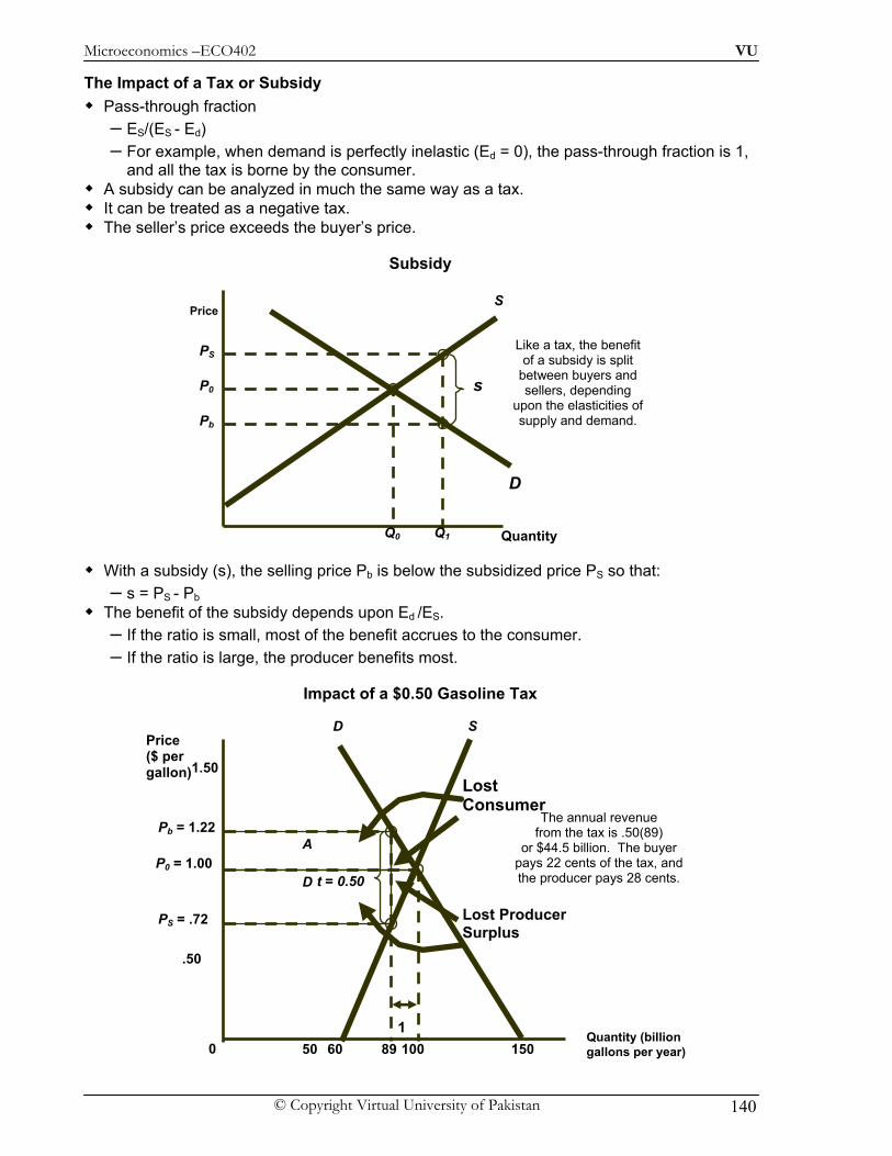
Microeconomics –ECO402 VU
© Copyright Virtual University of Pakistan 140
The Impact of a Tax or Subsidy Pass-through fraction
– ES/(ES - Ed) – For example, when demand is perfectly inelastic (Ed = 0), the pass-through fraction is 1,
and all the tax is borne by the consumer. A subsidy can be analyzed in much the same way as a tax. It can be treated as a negative tax. The seller’s price exceeds the buyer’s price.
Subsidy
With a subsidy (s), the selling price Pb is below the subsidized price PS so that: – s = PS - Pb
The benefit of the subsidy depends upon Ed /ES. – If the ratio is small, most of the benefit accrues to the consumer. – If the ratio is large, the producer benefits most.
Impact of a $0.50 Gasoline Tax
D
S
Quantity
Price
P0
Q0 Q1
PS
Pb
s
Like a tax, the benefit of a subsidy is split
between buyers and sellers, depending
upon the elasticities of supply and demand.
S D
60
D
A
Lost Consumer
Lost Producer Surplus
PS = .72
Pb = 1.22
Quantity (billion gallons per year)
Price ($ per gallon)
0 50 150
.50
100
P0 = 1.00
1.50
89
t = 0.50
1
The annual revenue from the tax is .50(89)
or $44.5 billion. The buyer pays 22 cents of the tax, and the producer pays 28 cents.
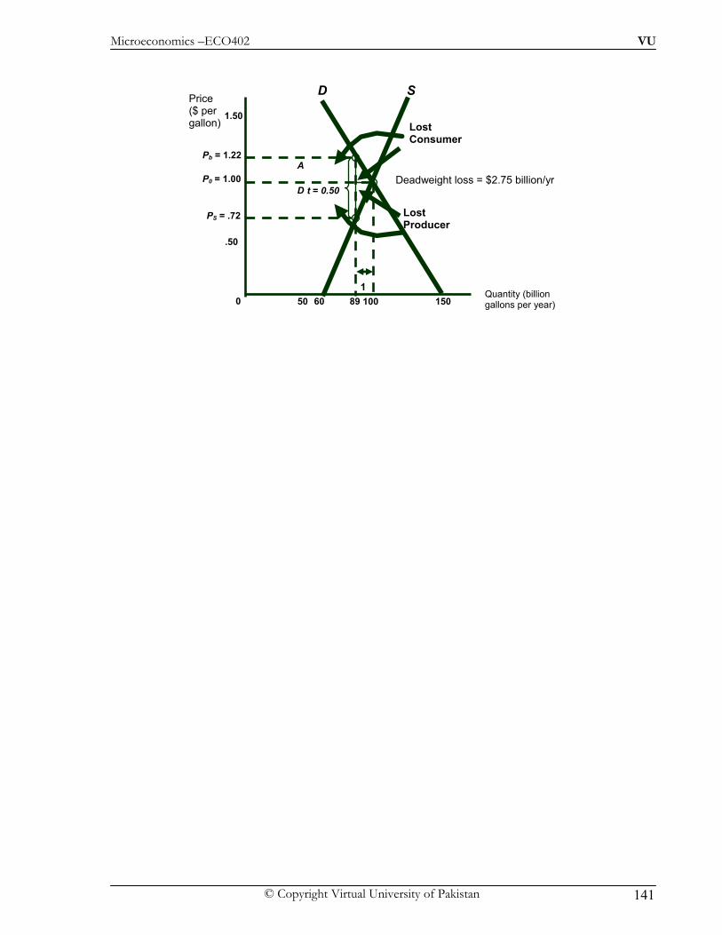
Microeconomics –ECO402 VU
© Copyright Virtual University of Pakistan 141
SD
60
D
A
Lost Consumer
Lost Producer
PS = .72
Pb = 1.22
Price ($ per gallon)
0 50 150
.50
100
P0 = 1.00
1.50
89
t = 0.50
1
Deadweight loss = $2.75 billion/yr
Quantity (billion gallons per year)
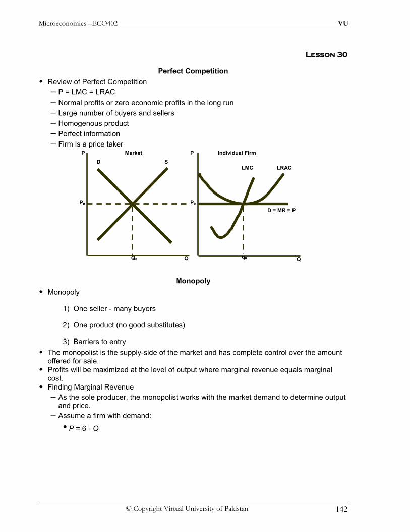
Microeconomics –ECO402 VU
© Copyright Virtual University of Pakistan 142
Lesson 30
Perfect Competition Review of Perfect Competition
– P = LMC = LRAC – Normal profits or zero economic profits in the long run – Large number of buyers and sellers – Homogenous product – Perfect information – Firm is a price taker
Monopoly Monopoly
1) One seller - many buyers
2) One product (no good substitutes)
3) Barriers to entry The monopolist is the supply-side of the market and has complete control over the amount
offered for sale. Profits will be maximized at the level of output where marginal revenue equals marginal
cost. Finding Marginal Revenue
– As the sole producer, the monopolist works with the market demand to determine output and price.
– Assume a firm with demand:
• P = 6 - Q
Q Q
P PMarket Individual FirmD S
Q0
P0 P0
D = MR = P
q0
LRAC LMC
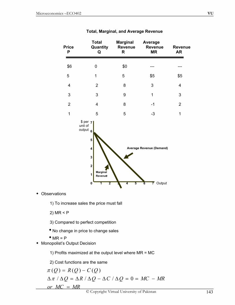
Microeconomics –ECO402 VU
© Copyright Virtual University of Pakistan 143
Total, Marginal, and Average Revenue
Total Marginal Average Price Quantity Revenue Revenue Revenue
P Q R MR AR
$6 0 $0 --- ---
5 1 5 $5 $5
4 2 8 3 4
3 3 9 1 3
2 4 8 -1 2
1 5 5 -3 1
Observations
1) To increase sales the price must fall
2) MR < P
3) Compared to perfect competition
• No change in price to change sales
• MR = P Monopolist’s Output Decision
1) Profits maximized at the output level where MR = MC
2) Cost functions are the same
Output 0
1
2
3
$ per unit of output
1 2 3 4 5 6 7
4
5
6
7
Average Revenue (Demand)
Marginal Revenue
MRMCorMRMCQCQRQ
QCQRQ
=−==ΔΔ−ΔΔ=ΔΔ
−=0///
)()()(π
π

Microeconomics –ECO402 VU
© Copyright Virtual University of Pakistan 144
Maximizing Profit When Marginal Revenue Equals Marginal Cost The Monopolist’s Output Decision
– At output levels below MR = MC the decrease in revenue is greater than the decrease in cost (MR > MC).
– At output levels above MR = MC the increase in cost is greater than the decrease in revenue (MR < MC)
Monopoly
The Monopolist’s Output Decision – An Example
• By setting marginal revenue equal to marginal cost, it can be verified that profit is maximized at P = $30 and Q = 10.
• This can be seen graphically:
Example of Profit Maximization
Lost profit
P1
Q
Lost profit
MC
A
Quantity
$ per unit of output
D = AR
M
P*
Q
P2
Q
Quantity
$
0 5 10 15 20
100
150
200
300
400
50
R
Profitst
t
c
c
C

Microeconomics –ECO402 VU
© Copyright Virtual University of Pakistan 145
Observations
– Slope of rr’ = slope cc’ and they are parallel at 10 units – Profits are maximized at 10 units – P = $30, Q = 10, TR = P x Q= $300 – AC = $15, Q = 10, TC = AC x Q = 150
– Profit = TR - TC • $150 = $300 - $150
Observations
– AC = $15, Q = 10, TC = AC x Q =150
– Profit = TR = TC = $300 - $150= $150 or
– Profit = (P-AC) x Q = ($30 -$15)(10) = $150
Profit
AR
MR
MC
AC
Quantity
$/Q
0 5 10 15 20
10
20
30
40
15

Microeconomics –ECO402 VU
© Copyright Virtual University of Pakistan 146
Lesson 31
A Rule of Thumb for Pricing
– We want to translate the condition that marginal revenue should equal marginal cost into a rule of thumb that can be more easily applied in practice.
– This can be demonstrated using the following steps:
( )( ) 14 .
15 .
d
d
Q PP Q E
M R P PE
Δ =Δ
= +⎛ ⎞⎜ ⎟⎝ ⎠
= the markup over MC as a percentage of price (P-MC)/P 8. The markup should equal the inverse of the elasticity of demand.
( )
( )
9. 11
4 9
9 9 $12
.7511 4
d
d
MCP
E
AssumeE MC
P
=+
= − =
= = =+ −
Monopoly pricing compared to perfect competition pricing: – Monopoly
P > MC – Perfect Competition
P = MC Monopoly pricing compared to perfect competition pricing:
⎟⎠⎞⎜
⎝⎛
ΔΔ⎟
⎠⎞⎜
⎝⎛=
⎟⎟⎠
⎞⎜⎜⎝
⎛ΔΔ
⎟⎠⎞
⎜⎝⎛+=
ΔΔ
+=
ΔΔ
=ΔΔ
=
PQ
QPE
QP
PQPP
QPQPMR
QPQ
QRMR
d.3
.2
)(.1
( )D
DD
E11MCP
EE1P P
MC MR @ maximized is
+=
−=⎥⎦
⎤⎢⎣
⎡+
=
1
.6 π
dE1.7 −

Microeconomics –ECO402 VU
© Copyright Virtual University of Pakistan 147
– The more elastic the demand the closer price is to marginal cost. – If Ed is a large negative number, price is close to marginal cost and vice versa.
A Monopolist’s Pricing The Monopolist’s Output Decision
– Price of Medicine A = $3.50/daily dose – Price of Medicine B and Medicine C = $1.50 - $2.25/daily dose – MC of Medicine A = 30 - 40 cents/daily dose
♦The Monopolist’s Output Decision ♦Price of $3.50 is consistent with “the rule of thumb pricing”
Shifts in Demand – In perfect competition, the market supply curve is determined by marginal cost. – For a monopoly, output is determined by marginal cost and the shape of the demand
curve.
Shift in Demand Leads to Change in Price but Same Output
[ ] [ ]
( ) 89.3$09.35.
91.1
1.11135.
11
==−+
=−+
=+
=
MCE
MCPD
D2
MR2
D1
MR1
Quantity
MC $/Q
P2
P1
Q1= Q2
D
MR1
MC$/Q
MR2
D2P1 = P2
Q1 Q Quantity
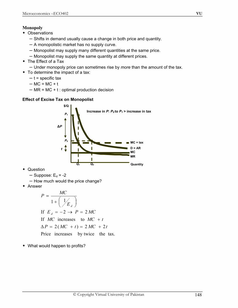
Microeconomics –ECO402 VU
© Copyright Virtual University of Pakistan 148
Monopoly
Observations – Shifts in demand usually cause a change in both price and quantity. – A monopolistic market has no supply curve. – Monopolist may supply many different quantities at the same price. – Monopolist may supply the same quantity at different prices.
The Effect of a Tax – Under monopoly price can sometimes rise by more than the amount of the tax.
To determine the impact of a tax: – t = specific tax – MC = MC + t – MR = MC + t : optimal production decision
Effect of Excise Tax on Monopolist
Question – Suppose: Ed = -2 – How much would the price change?
Answer
What would happen to profits?
tax. theby twice increases Price22)(2
toincreases If22If
11
tMCtMCPtMCMC
MCPEE
MCP
d
d
+=+=Δ+
=→−=
⎟⎠⎞⎜
⎝⎛+
=
Quantity
$/Q
MC D = AR
MR
Q0
P0 MC + tax
t
Q1
P1 Increase in P: P0 to P1 > increase in tax
ΔP

Microeconomics –ECO402 VU
© Copyright Virtual University of Pakistan 149
Lesson 32
Monopoly The Multiplant Firm
– For many firms, production takes place in two or more different plants whose operating cost can differ.
– Choosing total output and the output for each plant:
• The marginal cost in each plant should be equal.
• The marginal cost should equal the marginal revenue for each plant. – Algebraically:
– – Algebraically:
21
22
11
Output Total2Plant for Cost &Output &
1Plant for Cost &Output &
QQQCQCQ
T +==⇒⇒
0)()()(
1
1
11
2211
=ΔΔ
−Δ
Δ=
ΔΔ
−−=
QC
QPQ
Q
QCQCPQ
T
T
ππ
1
1
1
1
0)()()(
MCMRQCMC
QPQMR T
=
=ΔΔ
−Δ
Δ
21
2
1
MCMCMRMCMRMCMR
===−
Quantity
$/Q
D = AR
MR
MC1 MC2
MCT
MR*
Q1 Q Q
P*
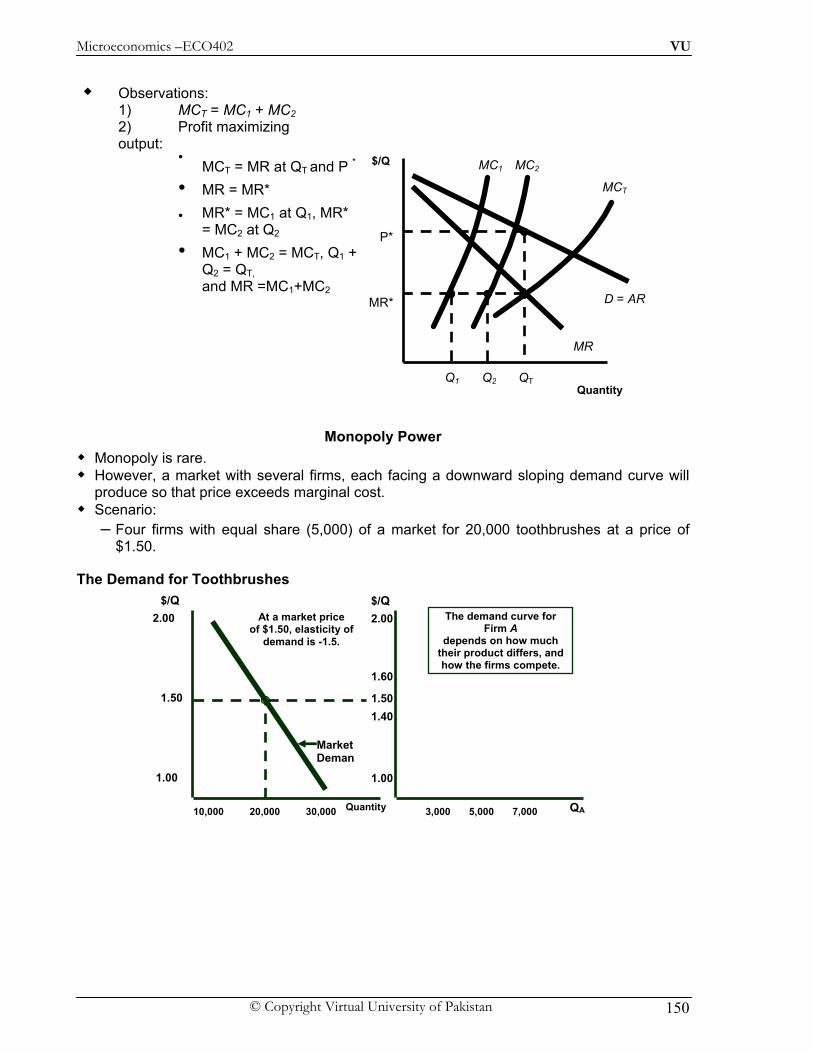
Microeconomics –ECO402 VU
© Copyright Virtual University of Pakistan 150
Monopoly Power
Monopoly is rare. However, a market with several firms, each facing a downward sloping demand curve will
produce so that price exceeds marginal cost. Scenario:
– Four firms with equal share (5,000) of a market for 20,000 toothbrushes at a price of $1.50.
The Demand for Toothbrushes
Quantity10,000
2.00
QA
$/Q $/Q
1.50
1.00
20,000 30,000 3,000 5,000 7,000
2.00
1.50
1.00
1.40
1.60
At a market price of $1.50, elasticity of
demand is -1.5.
Market Deman
The demand curve for Firm A
depends on how much their product differs, and how the firms compete.
Observations: 1) MCT = MC1 + MC2 2) Profit maximizing
output: • MCT = MR at QT and P *
• MR = MR*
• MR* = MC1 at Q1, MR* = MC2 at Q2
• MC1 + MC2 = MCT, Q1 + Q2 = QT, and MR =MC1+MC2
Quantity
$/Q
D = AR
MR
MC1 MC2
MCT
MR*
Q1 Q2 QT
P*

Microeconomics –ECO402 VU
© Copyright Virtual University of Pakistan 151
Measuring Monopoly Power – In perfect competition: P = MR = MC – Monopoly power: P > MC
Lerner’s Index of Monopoly Power – L = (P - MC)/P
• The larger the value of L (between 0 and 1) the greater the monopoly power. – L is expressed in terms of Ed
• L = (P - MC)/P = -1/Ed
• Ed is elasticity of demand for a firm, not the market Monopoly power does not guarantee profits. Profit depends on average cost relative to price. The Rule of Thumb for Pricing
– Pricing for any firm with monopoly power
• If Ed is large, markup is small
• If Ed is small, markup is large
Elasticity of Demand and Price Markup
( )dEMCP
11 +=
At a market price of $1.50, elasticity of
demand is -1.5.
Quantity10,000
2.00
QA
$/Q $/Q
1.50
1.00
20,000 30,000 3,000 5,000 7,000
2.00
1.50
1.00
1.40
1.60
DA
MR
Market Demand
Firm A sees a much more elastic demand curve due to competition--Ed = -.6. Still
Firm A has some monopoly power and charges a price
which exceeds MC.
MC
$/Q $/Q
Quantity Quantity
A
M
M
A
M M
Q* Q*
P*
P*
P*-MC
The more elastic is demand, the less the
markup.
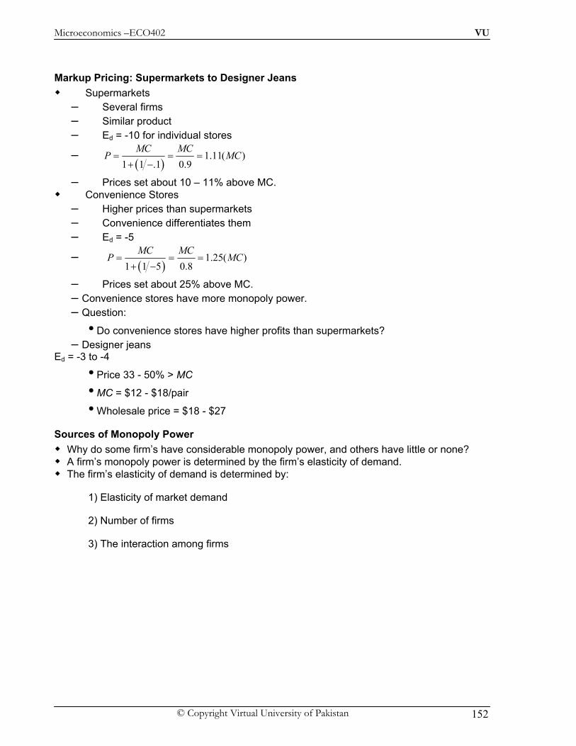
Microeconomics –ECO402 VU
© Copyright Virtual University of Pakistan 152
Markup Pricing: Supermarkets to Designer Jeans Supermarkets
– Several firms – Similar product – Ed = -10 for individual stores
– ( )
1.11( )1 1 .1 0.9
MC MCP MC= = =
+ −
– Prices set about 10 – 11% above MC. Convenience Stores
– Higher prices than supermarkets – Convenience differentiates them – Ed = -5
– ( )
1.25( )1 1 5 0.8
MC MCP MC= = =
+ −
– Prices set about 25% above MC. – Convenience stores have more monopoly power. – Question:
• Do convenience stores have higher profits than supermarkets? – Designer jeans
Ed = -3 to -4
• Price 33 - 50% > MC
• MC = $12 - $18/pair
• Wholesale price = $18 - $27
Sources of Monopoly Power Why do some firm’s have considerable monopoly power, and others have little or none? A firm’s monopoly power is determined by the firm’s elasticity of demand. The firm’s elasticity of demand is determined by:
1) Elasticity of market demand
2) Number of firms
3) The interaction among firms
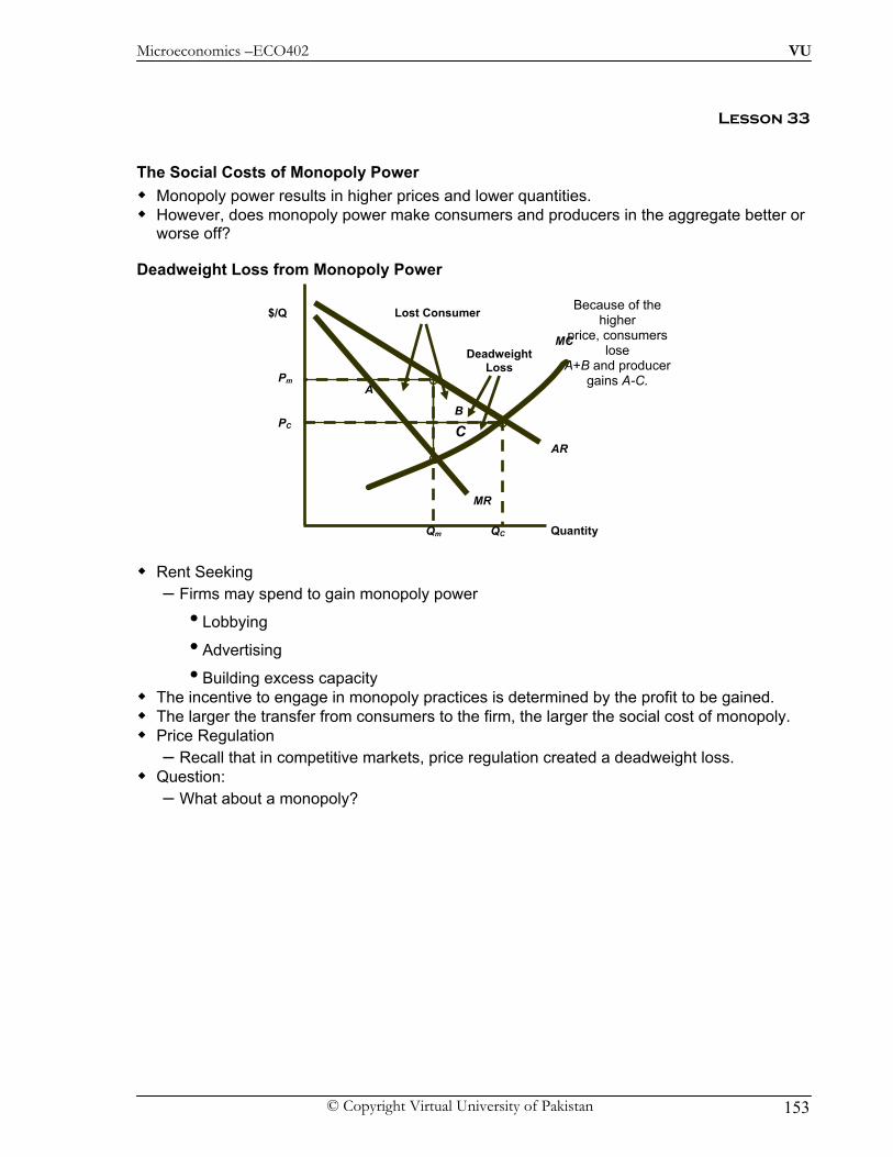
Microeconomics –ECO402 VU
© Copyright Virtual University of Pakistan 153
Lesson 33
The Social Costs of Monopoly Power Monopoly power results in higher prices and lower quantities. However, does monopoly power make consumers and producers in the aggregate better or
worse off?
Deadweight Loss from Monopoly Power
Rent Seeking – Firms may spend to gain monopoly power
• Lobbying
• Advertising
• Building excess capacity The incentive to engage in monopoly practices is determined by the profit to be gained. The larger the transfer from consumers to the firm, the larger the social cost of monopoly. Price Regulation
– Recall that in competitive markets, price regulation created a deadweight loss. Question:
– What about a monopoly?
B
A
Lost Consumer
Deadweight Loss
Because of the higher
price, consumers lose
A+B and producer gains A-C.
C
Quantity
AR
MR
MC
QC
PC
Pm
Qm
$/Q
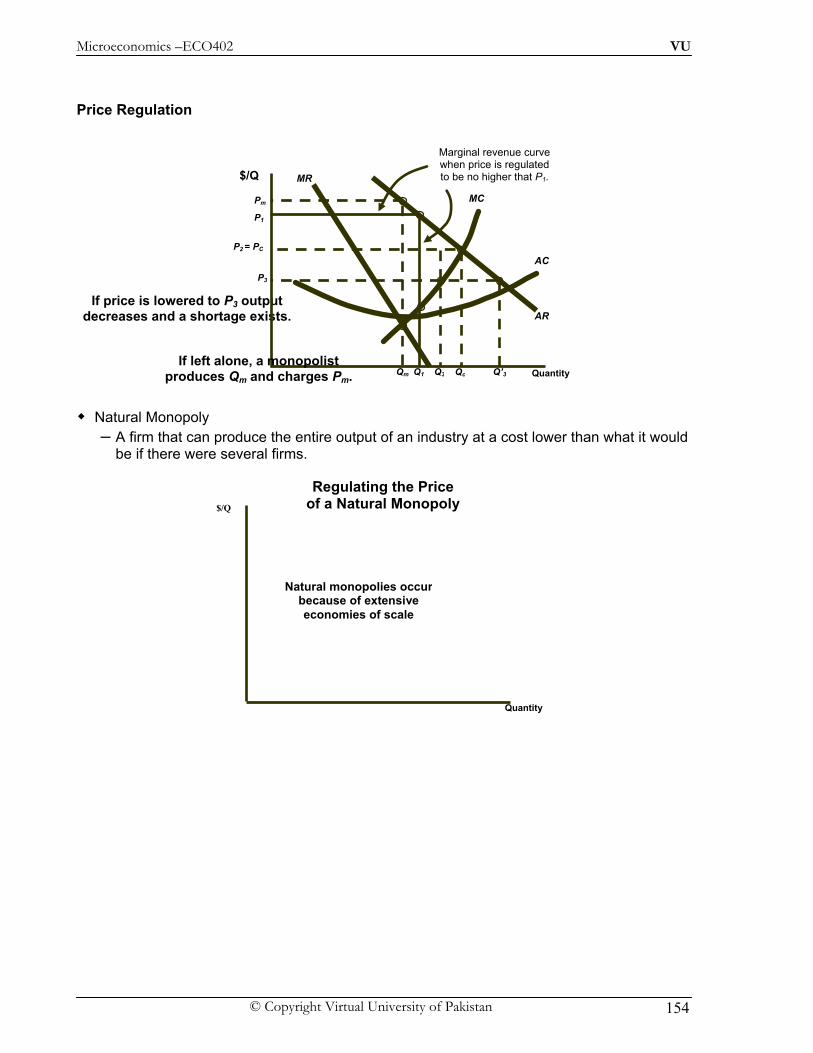
Microeconomics –ECO402 VU
© Copyright Virtual University of Pakistan 154
Price Regulation
Natural Monopoly – A firm that can produce the entire output of an industry at a cost lower than what it would
be if there were several firms.
Regulating the Price of a Natural Monopoly
$/Q
Natural monopolies occurbecause of extensive economies of scale
Quantity
If price is lowered to P3 output decreases and a shortage exists. AR
MR
MCPm
Qm
AC
P1
Q1
Marginal revenue curve when price is regulated to be no higher that P1.
If left alone, a monopolist produces Qm and charges Pm.
$/Q
Quantity
P2 = PC
Qc
P3
Q3 Q’3
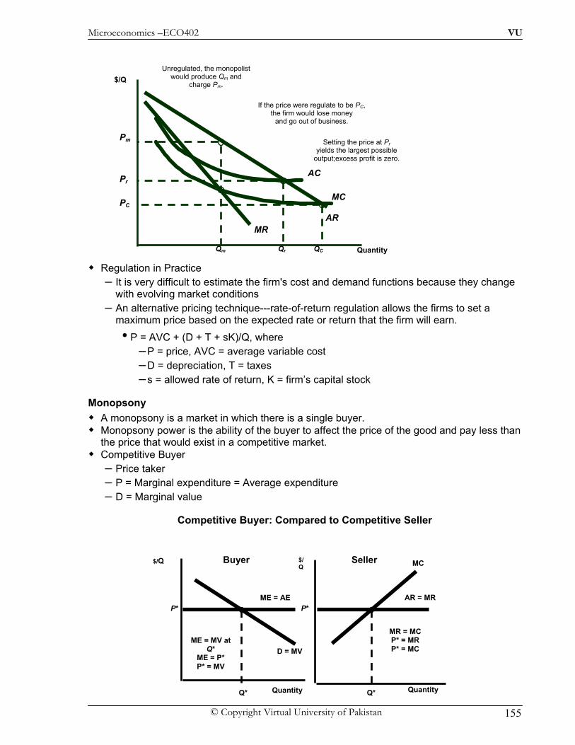
Microeconomics –ECO402 VU
© Copyright Virtual University of Pakistan 155
Regulation in Practice – It is very difficult to estimate the firm's cost and demand functions because they change
with evolving market conditions – An alternative pricing technique---rate-of-return regulation allows the firms to set a
maximum price based on the expected rate or return that the firm will earn.
• P = AVC + (D + T + sK)/Q, where – P = price, AVC = average variable cost – D = depreciation, T = taxes – s = allowed rate of return, K = firm’s capital stock
Monopsony A monopsony is a market in which there is a single buyer. Monopsony power is the ability of the buyer to affect the price of the good and pay less than
the price that would exist in a competitive market. Competitive Buyer
– Price taker – P = Marginal expenditure = Average expenditure – D = Marginal value
Competitive Buyer: Compared to Competitive Seller
MC
AC
ARMR
$/Q
Quantity
Setting the price at Pr yields the largest possible
output;excess profit is zero.
Qr
Pr
PC
QC
If the price were regulate to be PC, the firm would lose money
and go out of business.
Pm
Qm
Unregulated, the monopolist would produce Qm and
charge Pm.
Quantity Quantity
$/Q $/Q
AR = MR
D = MV
ME = AE P*
Q*
ME = MV at Q*
ME = P* P* = MV
P*
Q*
MC
MR = MC P* = MR P* = MC
Buyer Seller

Microeconomics –ECO402 VU
© Copyright Virtual University of Pakistan 156
Monopsonist Buyer
Monopoly and Monopsony
ME
S = AE
The market supply curve is the monopsonist’s average expenditure curve
Quantity
$/Q
MV
Q*m
P*m
Monopsony
•ME > P & above S
PC Competitive
•P = PC
•Q = QC
QC
Quantity
AR
MR
MC
$/Q
QC
PC
Monopoly Note: MR = MC;
AR > MC; P > MC
P*
Q*
Quantity
$/Q
MV
ME
S = AE
Q*
P*
PC
QC
Monopsony Note: ME = MV;
ME > AE; MV > P
Microeconomics –ECO402 VU
© Copyright Virtual University of Pakistan 157
Monopoly
– MR < P
– P > MC
– Qm < QC
– Pm > PC
Monopsony
– ME > P
– P < MV
– Qm < QC
– Pm < PC
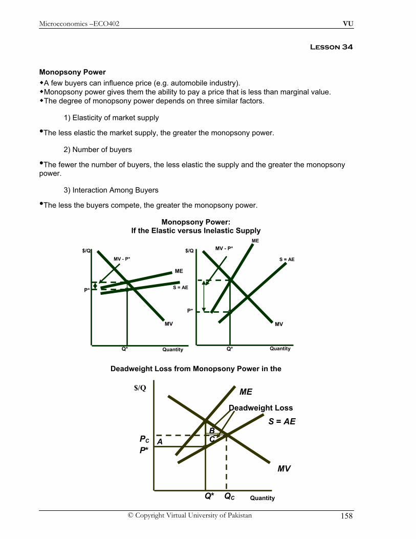
Microeconomics –ECO402 VU
© Copyright Virtual University of Pakistan 158
Lesson 34
Monopsony Power A few buyers can influence price (e.g. automobile industry). Monopsony power gives them the ability to pay a price that is less than marginal value. The degree of monopsony power depends on three similar factors.
1) Elasticity of market supply
•The less elastic the market supply, the greater the monopsony power.
2) Number of buyers
•The fewer the number of buyers, the less elastic the supply and the greater the monopsony power.
3) Interaction Among Buyers
•The less the buyers compete, the greater the monopsony power.
Monopsony Power: If the Elastic versus Inelastic Supply
Deadweight Loss from Monopsony Power in the
ME
S = AE
ME
S = AE
Quantity Quantity
$/Q $/Q
MV MV
Q*
P*
MV - P*
P*
Q*
MV - P*
A
Quantity
$/Q
MV
ME
S = AE
Q*
P* PC
QC
BC
Deadweight Loss
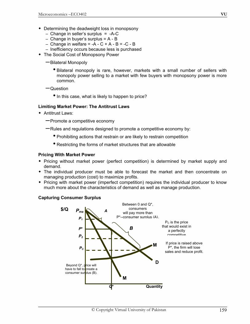
Microeconomics –ECO402 VU
© Copyright Virtual University of Pakistan 159
Determining the deadweight loss in monopsony
– Change in seller’s surplus = -A-C – Change in buyer’s surplus = A - B – Change in welfare = -A - C + A - B = -C - B – Inefficiency occurs because less is purchased
The Social Cost of Monopsony Power
– Bilateral Monopoly
• Bilateral monopoly is rare, however, markets with a small number of sellers with monopoly power selling to a market with few buyers with monopsony power is more common.
– Question
• In this case, what is likely to happen to price?
Limiting Market Power: The Antitrust Laws Antitrust Laws:
– Promote a competitive economy
– Rules and regulations designed to promote a competitive economy by:
• Prohibiting actions that restrain or are likely to restrain competition
• Restricting the forms of market structures that are allowable
Pricing With Market Power Pricing without market power (perfect competition) is determined by market supply and
demand. The individual producer must be able to forecast the market and then concentrate on
managing production (cost) to maximize profits. Pricing with market power (imperfect competition) requires the individual producer to know
much more about the characteristics of demand as well as manage production.
Capturing Consumer Surplus
Quantity
$/Q
D
M
Pma
M If price is raised above P*, the firm will lose
sales and reduce profit. PC
PC is the price that would exist in
a perfectly competitive
A
P*
Q*
P1
Between 0 and Q*, consumers
will pay more than P*--consumer surplus (A).
BP2
Beyond Q*, price will have to fall to create a consumer surplus (B).
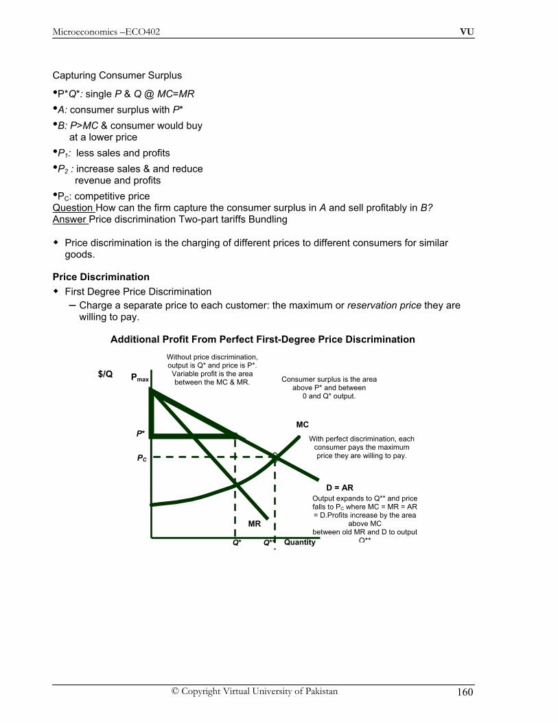
Microeconomics –ECO402 VU
© Copyright Virtual University of Pakistan 160
Capturing Consumer Surplus
•P*Q*: single P & Q @ MC=MR •A: consumer surplus with P* •B: P>MC & consumer would buy at a lower price •P1: less sales and profits •P2 : increase sales & and reduce revenue and profits •PC: competitive price Question How can the firm capture the consumer surplus in A and sell profitably in B? Answer Price discrimination Two-part tariffs Bundling
Price discrimination is the charging of different prices to different consumers for similar goods.
Price Discrimination First Degree Price Discrimination
– Charge a separate price to each customer: the maximum or reservation price they are willing to pay.
Additional Profit From Perfect First-Degree Price Discrimination
P*
Q*
Without price discrimination, output is Q* and price is P*.
Variable profit is the area between the MC & MR.
Quantity
$/Q Pmax
With perfect discrimination, each consumer pays the maximum price they are willing to pay.
Consumer surplus is the area above P* and between
0 and Q* output.
D = AR
MR
MC
Output expands to Q** and price falls to PC where MC = MR = AR = D.Profits increase by the area
above MC between old MR and D to output
Q**Q**
PC
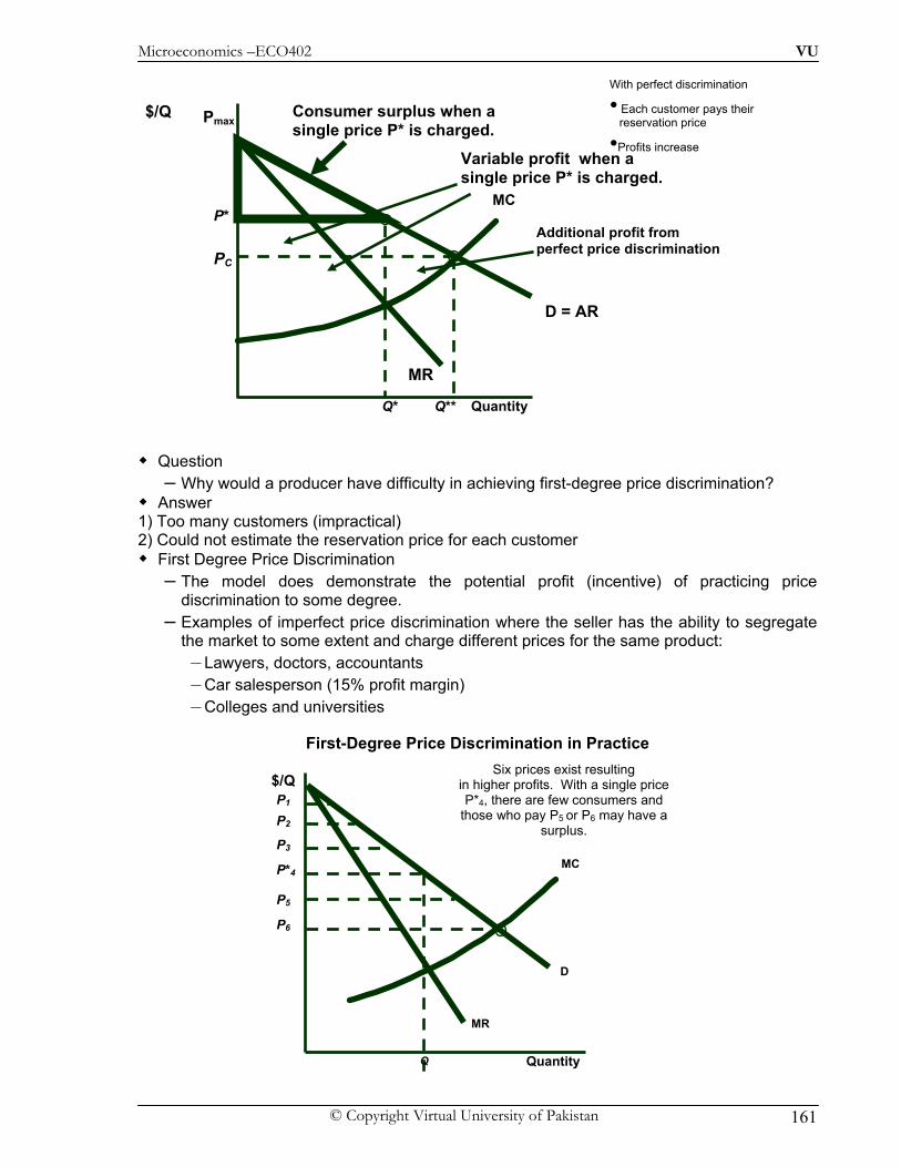
Microeconomics –ECO402 VU
© Copyright Virtual University of Pakistan 161
Question
– Why would a producer have difficulty in achieving first-degree price discrimination? Answer
1) Too many customers (impractical) 2) Could not estimate the reservation price for each customer
First Degree Price Discrimination – The model does demonstrate the potential profit (incentive) of practicing price
discrimination to some degree. – Examples of imperfect price discrimination where the seller has the ability to segregate
the market to some extent and charge different prices for the same product: – Lawyers, doctors, accountants – Car salesperson (15% profit margin) – Colleges and universities
First-Degree Price Discrimination in Practice
With perfect discrimination
• Each customer pays their reservation price
•Profits increase
Quantity
D
MR
MC
$/Q
P2
P3
P*4
P5
P6
P1
Six prices exist resulting in higher profits. With a single price P*4, there are few consumers and
those who pay P5 or P6 may have a surplus.
Q
P*
Q*
Consumer surplus when a single price P* is charged.
Variable profit when a single price P* is charged.
Additional profit from perfect price discrimination
Quantity
$/Q Pmax
D = AR
MR
MC
Q**
PC

Microeconomics –ECO402 VU
© Copyright Virtual University of Pakistan 162
Second-Degree Price Discrimination Economies of scale permit: •Increase consumer welfare •Higher profits
Quantity
$/Q
D
MR
MC
AC
P0
Q0
Without discrimination: P = P0 and Q = Q0. With second-
degree discrimination there are three
prices P1, P2, and P3. (e.g. electric utilities)
P1
Q1
1st
P2
Q2
P3
Q3
2nd 3rd
Second-degree price discrimination is pricing
according to quantity consumed--or in blocks.
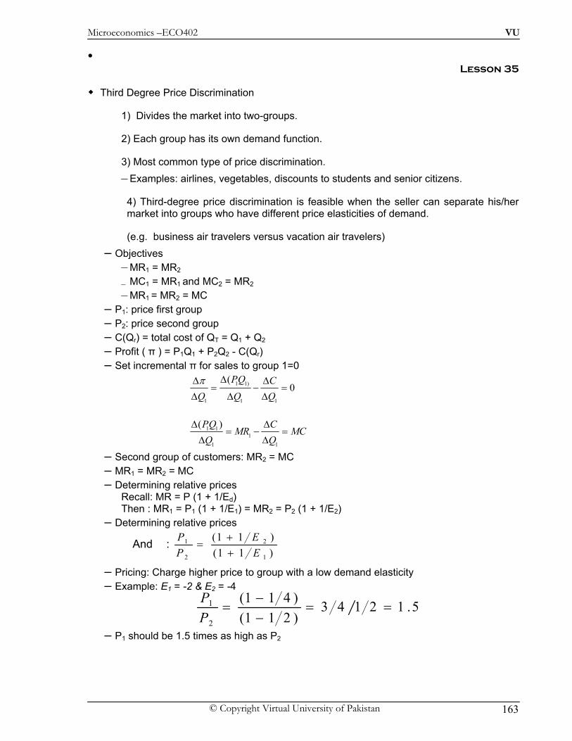
Microeconomics –ECO402 VU
© Copyright Virtual University of Pakistan 163
• Lesson 35
Third Degree Price Discrimination
1) Divides the market into two-groups.
2) Each group has its own demand function.
3) Most common type of price discrimination. – Examples: airlines, vegetables, discounts to students and senior citizens.
4) Third-degree price discrimination is feasible when the seller can separate his/her market into groups who have different price elasticities of demand.
(e.g. business air travelers versus vacation air travelers) – Objectives
– MR1 = MR2 – MC1 = MR1 and MC2 = MR2
– MR1 = MR2 = MC – P1: price first group – P2: price second group – C(Qr) = total cost of QT = Q1 + Q2 – Profit ( π ) = P1Q1 + P2Q2 - C(Qr) – Set incremental π for sales to group 1=0
1 1)
1 1 1
(0
PQ CQ Q Qπ ΔΔ Δ
= − =Δ Δ Δ
1 1
11 1
( )PQ CMR MC
Q QΔ Δ
= − =Δ Δ
– Second group of customers: MR2 = MC – MR1 = MR2 = MC – Determining relative prices
Recall: MR = P (1 + 1/Ed) Then : MR1 = P1 (1 + 1/E1) = MR2 = P2 (1 + 1/E2)
– Determining relative prices
– Pricing: Charge higher price to group with a low demand elasticity – Example: E1 = -2 & E2 = -4
– P1 should be 1.5 times as high as P2
)11()11(
1
2
2
1
EE
PP
++
= :And
5.12143)211()411(
2
1 ==−−
=PP
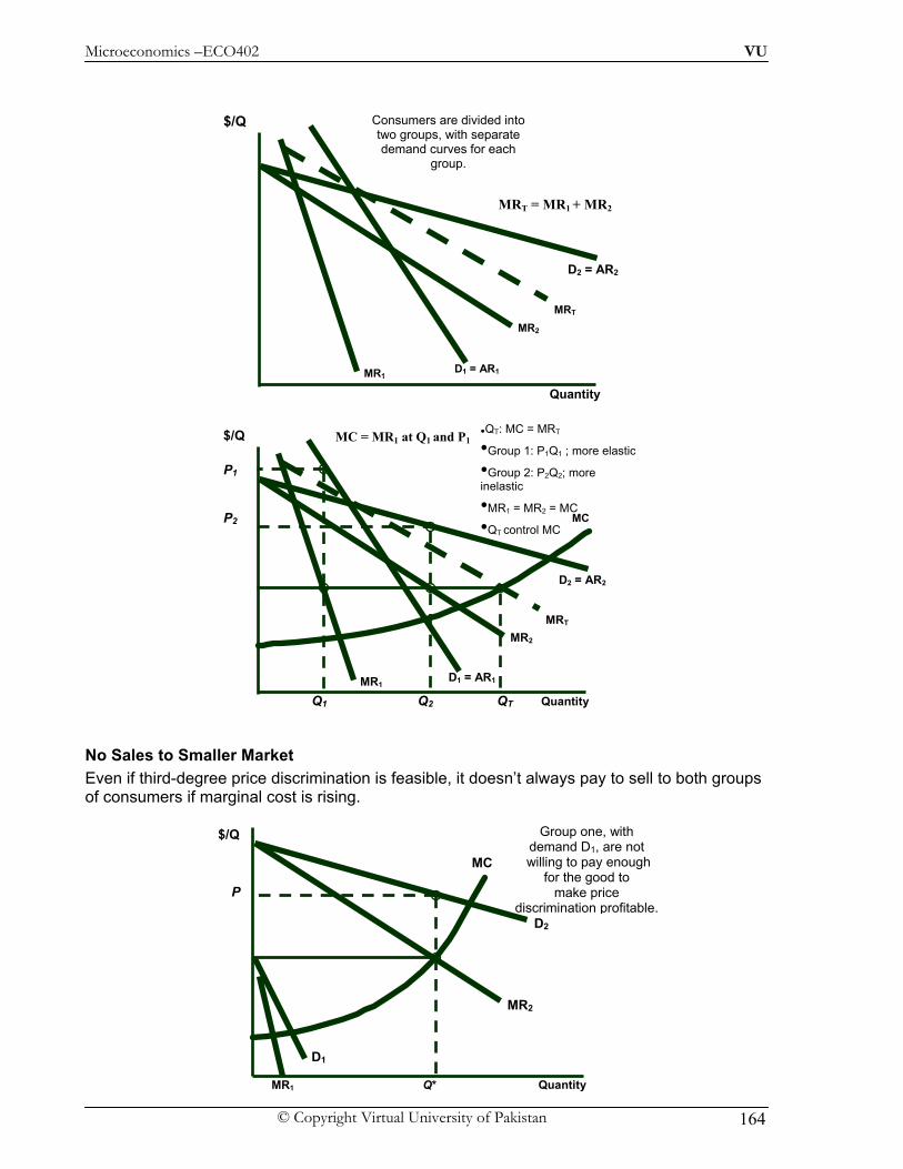
Microeconomics –ECO402 VU
© Copyright Virtual University of Pakistan 164
No Sales to Smaller Market Even if third-degree price discrimination is feasible, it doesn’t always pay to sell to both groups of consumers if marginal cost is rising.
Quantity
D2 = AR2
MR2
$/Q
D1 = AR1 MR1
Consumers are divided into two groups, with separate demand curves for each
group.
MRT
MRT = MR1 + MR2
Quantity
D2 = AR2
MR2
$/Q
D1 = AR1 MR1
MRT
MC
Q2
P2
QT
•QT: MC = MRT
•Group 1: P1Q1 ; more elastic
•Group 2: P2Q2; more inelastic
•MR1 = MR2 = MC
•QT control MC
Q1
P1
MC = MR1 at Q1 and P1
Quantity
D2
MR2
$/Q
MC
D1
MR1 Q*
P
Group one, with demand D1, are not
willing to pay enough for the good to
make price discrimination profitable.
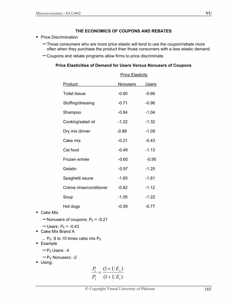
Microeconomics –ECO402 VU
© Copyright Virtual University of Pakistan 165
THE ECONOMICS OF COUPONS AND REBATES Price Discrimination
– Those consumers who are more price elastic will tend to use the coupon/rebate more often when they purchase the product than those consumers with a less elastic demand.
– Coupons and rebate programs allow firms to price discriminate.
Price Elasticities of Demand for Users Versus Nonusers of Coupons
Price Elasticity
Product Nonusers Users
Toilet tissue -0.60 -0.66
Stuffing/dressing -0.71 -0.96
Shampoo -0.84 -1.04
Cooking/salad oil -1.22 -1.32
Dry mix dinner -0.88 -1.09
Cake mix -0.21 -0.43
Cat food -0.49 -1.13
Frozen entrée -0.60 -0.95
Gelatin -0.97 -1.25
Spaghetti sauce -1.65 -1.81
Crème rinse/conditioner -0.82 -1.12
Soup -1.05 -1.22
Hot dogs -0.59 -0.77 Cake Mix
– Nonusers of coupons: PE = -0.21
– Users: PE = -0.43 Cake Mix Brand A
– PE: 8 to 10 times cake mix PE Example
– PE Users: -4
– PE Nonusers: -2 Using:
1 2
2 1
(1 1 )(1 1 )
P EP E
+=
+
Microeconomics –ECO402 VU
© Copyright Virtual University of Pakistan 166
Price of nonusers should be 1.5 times users
– Or, if cake mix sells for $1.50, coupons should be 50 cents
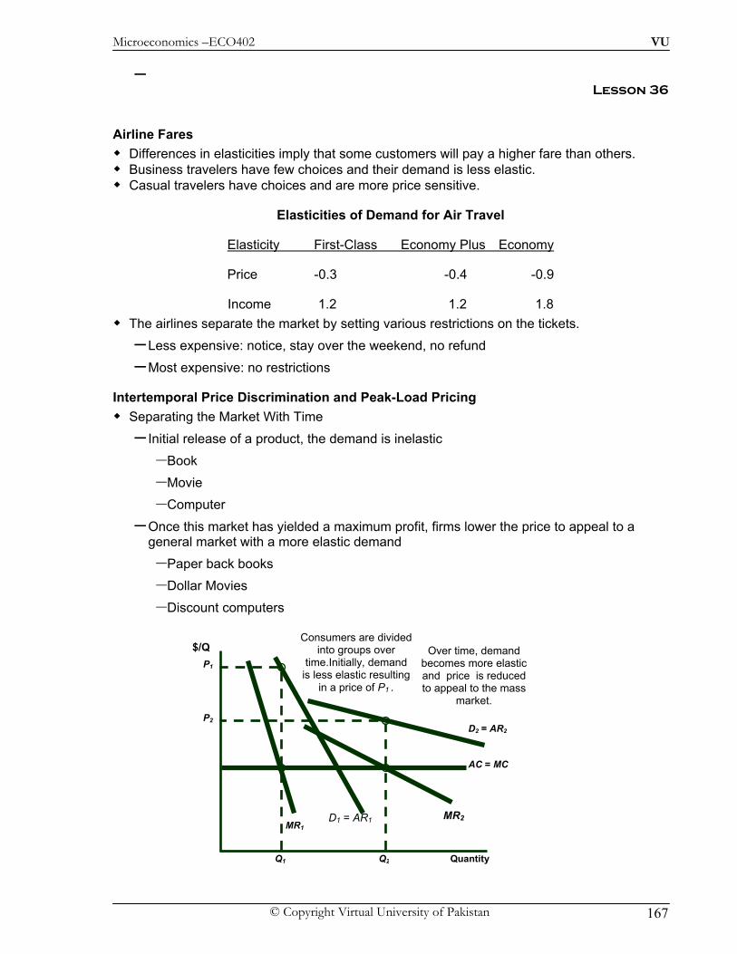
Microeconomics –ECO402 VU
© Copyright Virtual University of Pakistan 167
– Lesson 36
Airline Fares Differences in elasticities imply that some customers will pay a higher fare than others. Business travelers have few choices and their demand is less elastic. Casual travelers have choices and are more price sensitive.
Elasticities of Demand for Air Travel
Elasticity First-Class Economy Plus Economy
Price -0.3 -0.4 -0.9
Income 1.2 1.2 1.8 The airlines separate the market by setting various restrictions on the tickets.
– Less expensive: notice, stay over the weekend, no refund
– Most expensive: no restrictions
Intertemporal Price Discrimination and Peak-Load Pricing Separating the Market With Time
– Initial release of a product, the demand is inelastic – Book – Movie – Computer
– Once this market has yielded a maximum profit, firms lower the price to appeal to a general market with a more elastic demand – Paper back books – Dollar Movies – Discount computers
Quantity
AC = MC
$/Q Over time, demand becomes more elastic and price is reduced to appeal to the mass
market.
Q2
MR2
D2 = AR2
P2
D1 = AR1 MR1
P1
Q1
Consumers are divided into groups over
time.Initially, demand is less elastic resulting
in a price of P1 .

Microeconomics –ECO402 VU
© Copyright Virtual University of Pakistan 168
Peak-Load Pricing
– Demand for some products may peak at particular times. – Rush hour traffic – Electricity - summer season – Restaurants on weekends
– Capacity restraints will also increase MC.
– Increased MR and MC would indicate a higher price. – MR is not equal for each market because one market does not impact the other market.
How to Price a Best Selling Novel What Do You Think?
1) How would you arrive at the price for the initial release of the hardbound edition of a book?
2) How long do you wait to release the paperback edition? Could the popularity of the book impact your decision?
3) How do you determine the price for the paperback edition?
The Two-Part Tariff The purchase of some products and services can be separated into two decisions, and
therefore, two prices. Examples
1)Amusement Park
– Pay to enter – Pay for rides and food within the park
MR1
D1 = AR1
MC
P1
Q
Peak-load price = P1 .
Quantity
$/Q
MR2
D2 = AR2
Off- load price = P2 .
Q
P2
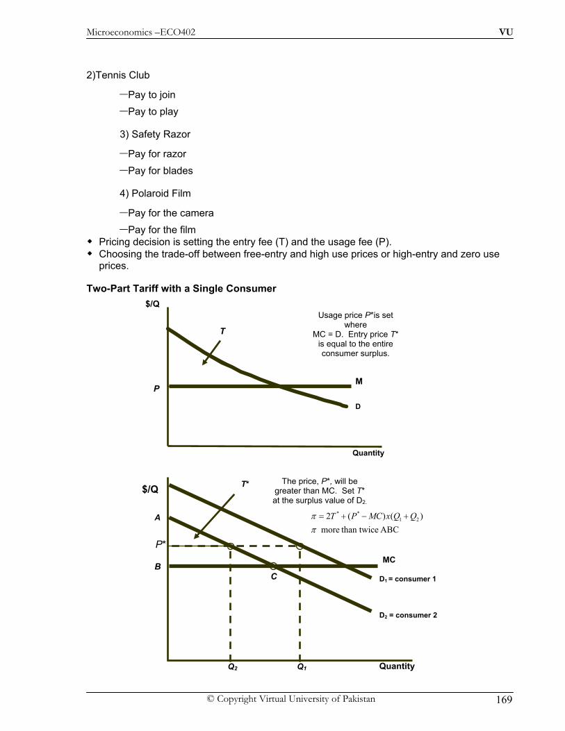
Microeconomics –ECO402 VU
© Copyright Virtual University of Pakistan 169
2)Tennis Club
– Pay to join – Pay to play
3) Safety Razor
– Pay for razor – Pay for blades
4) Polaroid Film
– Pay for the camera – Pay for the film
Pricing decision is setting the entry fee (T) and the usage fee (P). Choosing the trade-off between free-entry and high use prices or high-entry and zero use
prices.
Two-Part Tariff with a Single Consumer
Usage price P*is set where
MC = D. Entry price T* is equal to the entire consumer surplus.
T
Quantity
$/Q
MP
D
D2 = consumer 2
D1 = consumer 1
Q1 Q2
The price, P*, will be greater than MC. Set T* at the surplus value of D2.
T*
Quantity
$/Q
MC
A
B C
ABCethan twicmore )()(2 21
**
ππ QQxMCPT +−+=
P*
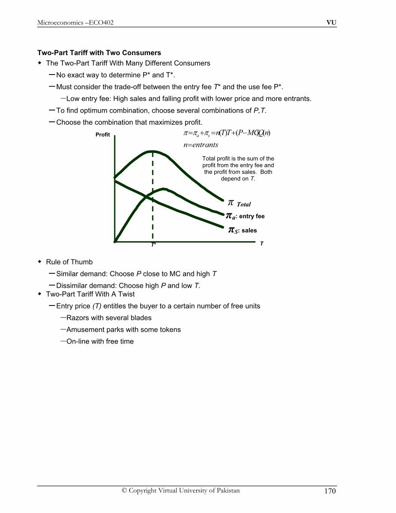
Microeconomics –ECO402 VU
© Copyright Virtual University of Pakistan 170
Two-Part Tariff with Two Consumers The Two-Part Tariff With Many Different Consumers
– No exact way to determine P* and T*.
– Must consider the trade-off between the entry fee T* and the use fee P*. – Low entry fee: High sales and falling profit with lower price and more entrants.
– To find optimum combination, choose several combinations of P,T. – Choose the combination that maximizes profit.
Rule of Thumb
– Similar demand: Choose P close to MC and high T
– Dissimilar demand: Choose high P and low T. Two-Part Tariff With A Twist
– Entry price (T) entitles the buyer to a certain number of free units – Razors with several blades – Amusement parks with some tokens – On-line with free time
T
Profit
πa: entry fee
πS: sales
T*
Total profit is the sum of the profit from the entry fee and the profit from sales. Both
depend on T.
entrantsnnQMCPTTnsa
=−+=+= )()()(πππ
π Total
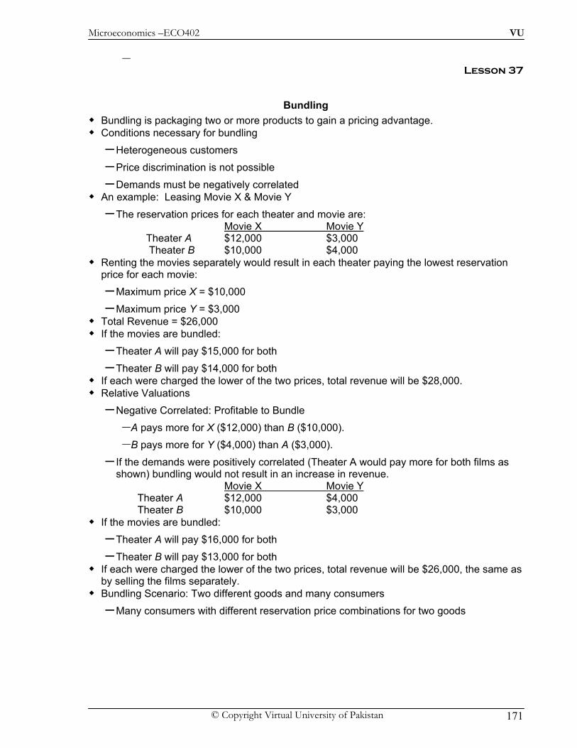
Microeconomics –ECO402 VU
© Copyright Virtual University of Pakistan 171
– Lesson 37
Bundling Bundling is packaging two or more products to gain a pricing advantage. Conditions necessary for bundling
– Heterogeneous customers
– Price discrimination is not possible
– Demands must be negatively correlated An example: Leasing Movie X & Movie Y
– The reservation prices for each theater and movie are: Movie X Movie Y
Theater A $12,000 $3,000 Theater B $10,000 $4,000
Renting the movies separately would result in each theater paying the lowest reservation price for each movie: – Maximum price X = $10,000
– Maximum price Y = $3,000 Total Revenue = $26,000 If the movies are bundled:
– Theater A will pay $15,000 for both
– Theater B will pay $14,000 for both If each were charged the lower of the two prices, total revenue will be $28,000. Relative Valuations
– Negative Correlated: Profitable to Bundle – A pays more for X ($12,000) than B ($10,000). – B pays more for Y ($4,000) than A ($3,000).
– If the demands were positively correlated (Theater A would pay more for both films as shown) bundling would not result in an increase in revenue.
Movie X Movie Y Theater A $12,000 $4,000 Theater B $10,000 $3,000
If the movies are bundled: – Theater A will pay $16,000 for both
– Theater B will pay $13,000 for both If each were charged the lower of the two prices, total revenue will be $26,000, the same as
by selling the films separately. Bundling Scenario: Two different goods and many consumers
– Many consumers with different reservation price combinations for two goods

Microeconomics –ECO402 VU
© Copyright Virtual University of Pakistan 172
Reservation Prices
Consumption Decisions When Products are Sold Separately
Consumption Decisions When Products are Bundled
r2 (reservation
price Good 2)
r1 (reservation priceGood 1)
$5
$10
$5 $10
$6
$3.25 $8.25
$3.25
Consumer A
ConsumerC
Consumer B
Consumer A is willing to pay up to
$3.25 for good 1 and up to $6 for good 2.
r2
r1
P2
II Consumers
buy
22
11
PRPR
><
P1
Consumers fall into four categories based on their reservation
price. IConsumers
buy
22
11
PRPR
>>
III
Consumers buy
22
11
PRPR
<<
IV
Consumers buy
22
11
PRPR
<>
r2
r1
Consumers buy the bundlewhen r1 + r2 > PB
(PB = bundle price). PB = r1 + r2 or r2 = PB - r1
Region 1: r > PB Region 2: r < PB
r2 = PB - r1
I
I
Consumers buy bundle
(r > PB)
Consumers do not buy bundle
(r < PB)
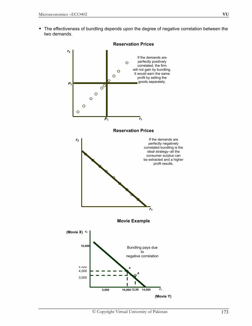
Microeconomics –ECO402 VU
© Copyright Virtual University of Pakistan 173
The effectiveness of bundling depends upon the degree of negative correlation between the
two demands.
Reservation Prices
Reservation Prices
Movie Example
r2
r1
P2
P1
If the demands are perfectly positively correlated, the firm
will not gain by bundling. It would earn the same
profit by selling the goods separately.
r2
r1
If the demands are perfectly negatively
correlated bundling is the ideal strategy--all the consumer surplus can
be extracted and a higher profit results.
r2
r1
Bundling pays due to
negative correlation
(Movie Y)
(Movie X)
5,000 14,00010,000
5 000
10,000
12,00
4,000
3,000
B
A

Microeconomics –ECO402 VU
© Copyright Virtual University of Pakistan 174
Lesson 38
Bundling Mixed Bundling
– Selling both as a bundle and separately Pure Bundling
– Selling only a package
Mixed Versus Pure Bundling
Mixed vs. Pure Bundling – Scenario
– Perfect negative correlation – Significant marginal cost
– Observations – Reservation price is below MC for some consumers – Mixed bundling induces the consumers to buy only goods for which their reservation
price is greater than MC
Bundling Example Sell Separately
– Consumers B,C, and D buy 1 and A buys 2 Pure Bundling
– Consumers A, B, C, and D buy the bundle Mixed Bundling
– Consumer D buys 1, A buys 2, and B & C buys the bundle
r2
r110 20 30 40 50 60 70 80 90 100
10
20
30
40
50
60
70
80
90
100
C2 = MC2C2 = 30
Consumer A, for example, has a reservation price for good 1 that is below marginal cost c1.
With mixed bundling, consumer A is induced to buy only good 2, while
consumer D is induced to buy only good 1, reducing the firm’s cost.
A
B
D
C
C1 = MC1 C1 = 20 With positive marginal
costs, mixed bundling may be more profitable
than pure bundling.

Microeconomics –ECO402 VU
© Copyright Virtual University of Pakistan 175
P1 P2 PB Profit
Sell separately $50 $90 ---- $150
Pure bundling ---- ---- $100 $200
Mixed bundling $89.95 $89.95 $100 $229.90
C1 = $20
C2 = $30 Sell Separately
– 3($50 - $20) + 1($90 - $30) = $150 Pure Bundling
– 4($100 - $20 - $30) = $200 Mixed Bundling
– ($89.95 - $20) + ($89.95 - $30) - 2($100 - $20 - $30) = $229.90 – C1 = $20 C2 = $30
Question
– If MC = 0, would mixed bundling still be the most profitable strategy with perfect negative correlation?
Mixed Bundling with Zero Marginal Costs
P1 P2 PB Profit Sell separately $80 $80 ---- $320 Pure bundling ---- ---- $100 $400
Mixed bundling $90 $90 $120 $420
r2
r1 20 40 60 80 100
20
40
60
80
100
120
120 In this example, consumers B and C
are willing to pay $20 more for the bundle than are consumers A and D. With
mixed bundling, the price of the bundle can be increased to $120. A & D can be
charged $90 for a single good.
C
1 9
1
9 AB
D

Microeconomics –ECO402 VU
© Copyright Virtual University of Pakistan 176
Bundling in Practice
– Automobile option packages
– Vacation travel
– Cable television Mixed Bundling in Practice
– Use of market surveys to determine reservation prices
– Design a pricing strategy from the survey results
The Complete Dinner vs. a la Carte: A Restaurant’s Pricing Problem
Pricing to match consumer preferences for various selections Mixed bundling allows the customer to get maximum utility from a given expenditure by
allowing a greater number of choices.
Bundling Tying
– Practice of requiring a customer to purchase one good in order to purchase another. – Examples
– Xerox machines and the paper – IBM mainframe and computer cards
– Allows the seller to meter the customer and use a two-part tariff to discriminate against the heavy user
– McDonald’s – Allows them to protect their brand name.
Advertising Assumptions
– Firm sets only one price – Firm knows Q(P,A)
– How quantity demanded depends on price and advertising
r2
r1
The firm can first choose a price for the bundle and then try individual
prices P1 and P2 until total profit is roughly maximized.
P2
PB
PBP1
The dots are estimates of reservation prices for a
representative sample of consumers.
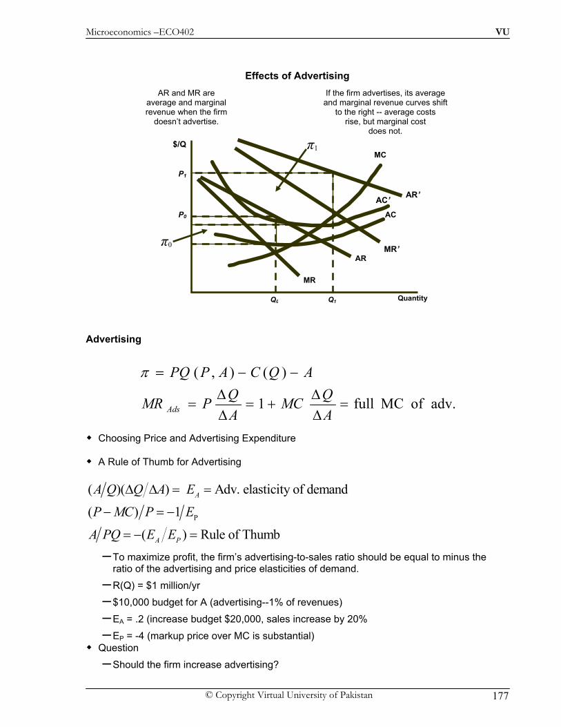
Microeconomics –ECO402 VU
© Copyright Virtual University of Pakistan 177
Effects of Advertising
Advertising
Choosing Price and Advertising Expenditure
A Rule of Thumb for Advertising
P
( )( ) Adv. elasticity of demand
( ) 1
( ) Rule of Thumb
A
A P
A Q Q A E
P MC P E
A PQ E E
Δ Δ = =
− = −
= − =
– To maximize profit, the firm’s advertising-to-sales ratio should be equal to minus the ratio of the advertising and price elasticities of demand.
– R(Q) = $1 million/yr – $10,000 budget for A (advertising--1% of revenues)
– EA = .2 (increase budget $20,000, sales increase by 20%
– EP = -4 (markup price over MC is substantial) Question
– Should the firm increase advertising?
Q0
P0
π0
Q1
P1
π1
AR
MR
AR and MR are average and marginal revenue when the firm
doesn’t advertise.
MC
If the firm advertises, its average and marginal revenue curves shift
to the right -- average costs rise, but marginal cost
does not.
AR’
MR’
AC’
Quantity
$/Q
AC
adv. of MC full1
)(),(
=ΔΔ
+=ΔΔ
=
−−=
AQMC
AQPMR
AQCAPPQ
Ads
π

Microeconomics –ECO402 VU
© Copyright Virtual University of Pakistan 178
YES
– A/PQ = -(2/-.4) = 5%
– Increase budget to $50,000 Questions
– When EA is large, do you advertise more or less?
– When EP is large, do you advertise more or less? Advertising: In Practice
– Estimate the level of advertising for each of the firms – Supermarkets EP= -10; EA = 0.1 to 0.3 – Convenience stores EP= -5; EA = very small – Designer jeans EP= -3 to -4; EA= 0.3 to 1 – Laundry detergents EP= -3 to -4; EA= very large

Microeconomics –ECO402 VU
© Copyright Virtual University of Pakistan 179
Lesson 39
MONOPOLISTIC COMPETITION Characteristics
1) Many firms
2) Free entry and exit
3) Differentiated product The amount of monopoly power depends on the degree of differentiation. Examples of this very common market structure include:
– Toothpaste – Soap – Cold remedies
Toothpaste – Brand J and monopoly power
• Suppose an MNC is the sole producer of Brand J
• Consumers can have a preference for Brand J---taste, reputation, decay preventing efficacy
• The greater the preference (differentiation) the higher the price. The Makings of Monopolistic Competition
– Two important characteristics
• Differentiated but highly substitutable products
• Free entry and exit
A Monopolistically Competitive Firm in the Short and Long Run
Observations (short-run) – Downward sloping demand--differentiated product – Demand is relatively elastic--good substitutes – MR < P – Profits are maximized when MR = MC
Quantity
$/Q
Quantity
$/QMC
AC
MC
AC
DSR
MRSR
DLR
MRLR
QSR
PSR
QLR
PLR
Short Run Long Run

Microeconomics –ECO402 VU
© Copyright Virtual University of Pakistan 180
– This firm is making economic profits
Observations (long-run) – Profits will attract new firms to the industry (no barriers to entry) – The old firm’s demand will decrease to DLR
– Firm’s output and price will fall – Industry output will rise – No economic profit (P = AC) – P > MC -- some monopoly power
Monopolistically Competitive vs. Perfectly Competitive Equilibrium
Monopolistic Competition and Economic Efficiency – The monopoly power (differentiation) yields a higher price than perfect competition. If
price was lowered to the point where MC = D, consumer surplus would increase by the shaded triangle.
– With no economic profits in the long run, the firm is still not producing at minimum AC and excess capacity exists.
Questions
1) If the market became competitive, what would happen to output and price?
2) Should monopolistic competition be regulated?
Monopolistic Competition in the Market for Colas and Coffee The markets for soft drinks and coffee illustrate the characteristics of monopolistic
competition.
Deadweight loss MC AC
$/Q
Quantity
$/Q
D =
QC
PC
MC AC
DLR
MRLR
QMC
P
Quantity
Perfect Competition Monopolistic Competition

Microeconomics –ECO402 VU
© Copyright Virtual University of Pakistan 181
Elasticities of Demand for Brands of Colas and Coffee Colas: Brand X -2.4
Brand Y - 5.2 to -5.7
Ground Coffee: Hills Brothers -7.1
Maxwell House -8.9
Chase and Sanborn -5.6
Questions
1) Why is the demand for Brand X more price inelastic than for Brand Y?
2) Is there much monopoly power in these two markets?
3) Define the relationship between elasticity and monopoly power.
Microeconomics –ECO402 VU
© Copyright Virtual University of Pakistan 182
Lesson 40
OLIGOPOLY Characteristics
– Small number of firms – Product differentiation may or may not exist – Barriers to entry
Examples – Automobiles – Steel – Aluminum – Petrochemicals – Electrical equipment – Computers
The barriers to entry are: – Natural
• Scale economies
• Patents
• Technology
• Name recognition – Strategic action
• Flooding the market
• Controlling an essential input Management Challenges
– Strategic actions – Rival behavior
Question – What are the possible rival responses to a 10% price cut by an automobile company?
Equilibrium in an Oligopolistic Market – In perfect competition, monopoly, and monopolistic competition the producers did not
have to consider a rival’s response when choosing output and price. – In oligopoly the producers must consider the response of competitors when choosing
output and price. – Defining Equilibrium
• Firms doing the best they can and have no incentive to change their output or price
• All firms assume competitors are taking rival decisions into account. Nash Equilibrium
– Each firm is doing the best it can given what its competitors are doing. The Cournot Model
– Duopoly
• Two firms competing with each other
• Homogenous good
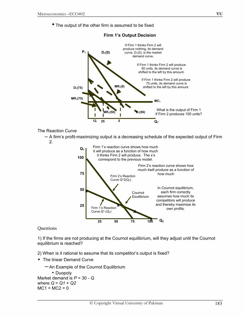
Microeconomics –ECO402 VU
© Copyright Virtual University of Pakistan 183
• The output of the other firm is assumed to be fixed
Firm 1’s Output Decision The Reaction Curve
– A firm’s profit-maximizing output is a decreasing schedule of the expected output of Firm 2.
Questions
1) If the firms are not producing at the Cournot equilibrium, will they adjust until the Cournot equilibrium is reached?
2) When is it rational to assume that its competitor’s output is fixed? The linear Demand Curve
– An Example of the Cournot Equilibrium • Duopoly
Market demand is P = 30 - Q where Q = Q1 + Q2 MC1 = MC2 = 0
D1(0)
MR1(0)
If Firm 1 thinks Firm 2 will produce nothing, its demand curve, D1(0), is the market
demand curve.
MC1
5
MR1(75)
D1(75)
12.
If Firm 1 thinks Firm 2 will produce 75 units, its demand curve is
shifted to the left by this amount.
Q1
P1
What is the output of Firm 1 if Firm 2 produces 100 units?D1(50) MR1(50)
25
If Firm 1 thinks Firm 2 will produce 50 units, its demand curve is
shifted to the left by this amount.
Firm 2’s Reaction Curve Q*2(Q2)
Firm 2’s reaction curve shows how much itwill produce as a function of
how much
Q2
Q1
25 50 75 100
25
50
75
100
Firm 1’s Reaction Curve Q*1(Q2)
x
xx
x
Firm 1’s reaction curve shows how much it will produce as a function of how much
it thinks Firm 2 will produce. The x’s correspond to the previous model.
In Cournot equilibrium, each firm correctly
assumes how much its competitors will produce and thereby maximize its
own profits.
Cournot Equilibrium

Microeconomics –ECO402 VU
© Copyright Virtual University of Pakistan 184
Duopoly Example
Profit Maximization with Collusion
– Collusion Curve • Q1 + Q2 = 15
–Shows all pairs of output Q1 and Q2 that maximizes total profits • Q1 = Q2 = 7.5
–Less output and higher profits than the Cournot equilibrium
First Mover Advantage- The Stackelberg Model
Assumptions – One firm can set output first – MC = 0 – Market demand is P = 30 - Q where Q = total output – Firm 1 sets output first and Firm 2 then makes an output decision
Firm 1 – Must consider the reaction of Firm 2
Firm 2
Q1
Q2
Firm 2’s Reaction Curve
3
1
Firm 1’s Reaction
1
3
1
1
Cournot
The demand curve is P = 30 - Q and
both firms have 0 marginal cost.
Q1
Q2
Firm 2’s Reaction Curve
3
1
Firm 1’s Reaction Curve
1
3
1
10
Cournot E ilib i
The demand curve is P = 30 - Q and
both firms have 0 marginal cost.
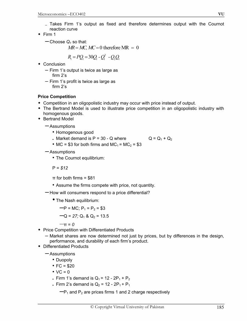
Microeconomics –ECO402 VU
© Copyright Virtual University of Pakistan 185
– Takes Firm 1’s output as fixed and therefore determines output with the Cournot reaction curve
Firm 1 – Choose Q1 so that:
21 1 1 1 2 1
0 therefore MR 0
30
MR MC, MC
R PQ Q - Q - Q Q
= = =
= =
Conclusion – Firm 1’s output is twice as large as
firm 2’s – Firm 1’s profit is twice as large as
firm 2’s
Price Competition Competition in an oligopolistic industry may occur with price instead of output. The Bertrand Model is used to illustrate price competition in an oligopolistic industry with
homogenous goods. Bertrand Model
– Assumptions • Homogenous good • Market demand is P = 30 - Q where Q = Q1 + Q2
• MC = $3 for both firms and MC1 = MC2 = $3
– Assumptions • The Cournot equilibrium:
P = $12
π for both firms = $81 • Assume the firms compete with price, not quantity.
– How will consumers respond to a price differential?
• The Nash equilibrium:
–P = MC; P1 = P2 = $3
–Q = 27; Q1 & Q2 = 13.5
–π = 0 Price Competition with Differentiated Products
– Market shares are now determined not just by prices, but by differences in the design, performance, and durability of each firm’s product.
Differentiated Products
– Assumptions • Duopoly • FC = $20 • VC = 0 • Firm 1’s demand is Q1
= 12 - 2P1 + P2
• Firm 2’s demand is Q2 = 12 - 2P1 + P1
–P1 and P2 are prices firms 1 and 2 charge respectively
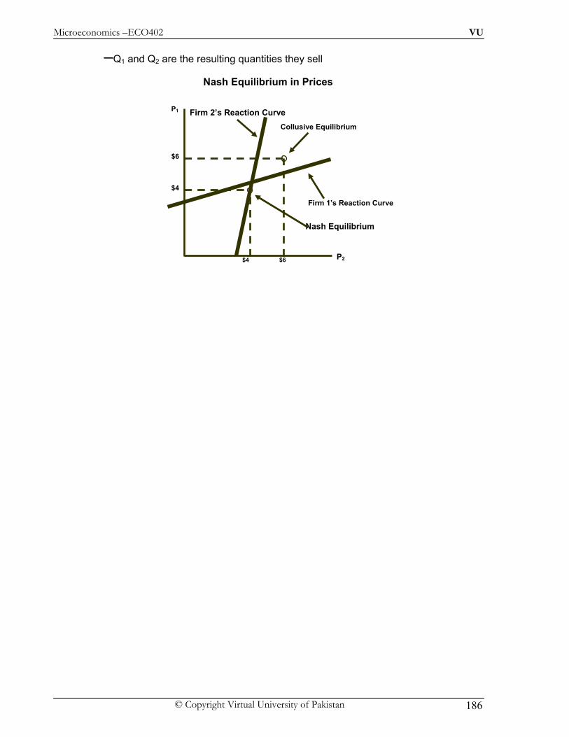
Microeconomics –ECO402 VU
© Copyright Virtual University of Pakistan 186
–Q1 and Q2 are the resulting quantities they sell
Nash Equilibrium in Prices
Firm 1’s Reaction Curve
P1
P2
Firm 2’s Reaction Curve
$4
$4
Nash Equilibrium
$6
$6
Collusive Equilibrium

Microeconomics –ECO402 VU
© Copyright Virtual University of Pakistan 187
Lesson 41
Competition Versus Collusion:
The Prisoners’ Dilemma Why wouldn’t each firm set the collusion price independently and earn the higher profits that
occur with explicit collusion? Assume:
Possible Pricing Outcomes:
Payoff Matrix for Pricing Game
These two firms are playing a non co-operative game. – Each firm independently does the best it can taking its competitor into account.
Question – Why will both firms both choose $4 when $6 will yield higher profits?
An example in game theory, called the Prisoners’ Dilemma, illustrates the problem oligopolistic firms face.
[ ]
[ ] 4$204)6)(2(12)6( 20
20$206)4)(2(12)4( 20
4$ 6$ $16 6$ :2 Firm 6$ :1 Firm
111
222
=−+−=−=
=−+−=−=
=====
QP
QPPPPP
π
π
π
16$ 6$ :Collusion12$ 4$ :mEquilibriu Nash
212 :Demands2' Firm
212 :Demands1' Firm
0$and20$
12
21
==
==
+−=
+−=
==
ππ
PP
PPQPPQ
VCFC
Firm 2
Firm 1
Charge $4 Charge $6
Charge $4
Charge $6
$12, $20,
$16, $4,
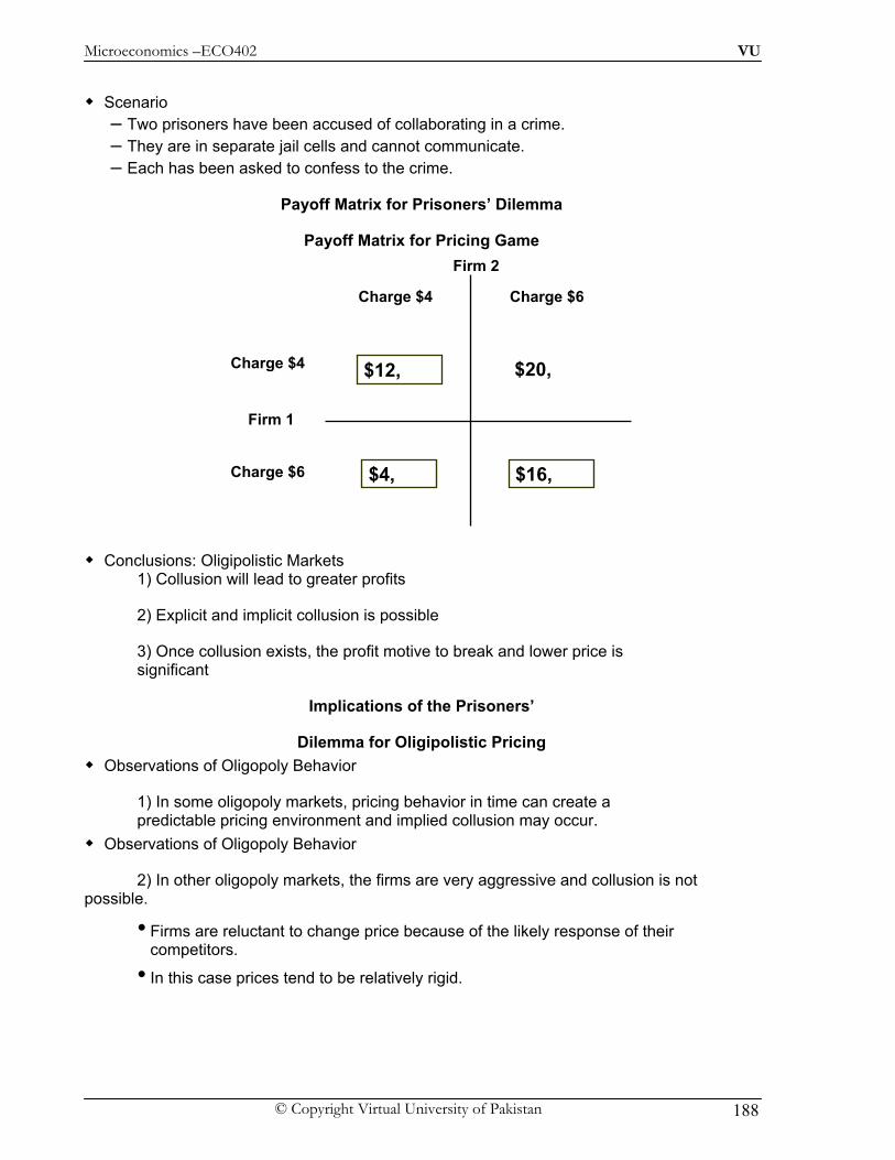
Microeconomics –ECO402 VU
© Copyright Virtual University of Pakistan 188
Scenario
– Two prisoners have been accused of collaborating in a crime. – They are in separate jail cells and cannot communicate. – Each has been asked to confess to the crime.
Payoff Matrix for Prisoners’ Dilemma
Payoff Matrix for Pricing Game
Conclusions: Oligipolistic Markets 1) Collusion will lead to greater profits
2) Explicit and implicit collusion is possible
3) Once collusion exists, the profit motive to break and lower price is significant
Implications of the Prisoners’
Dilemma for Oligipolistic Pricing Observations of Oligopoly Behavior
1) In some oligopoly markets, pricing behavior in time can create a predictable pricing environment and implied collusion may occur.
Observations of Oligopoly Behavior
2) In other oligopoly markets, the firms are very aggressive and collusion is not possible.
• Firms are reluctant to change price because of the likely response of their competitors.
• In this case prices tend to be relatively rigid.
Firm 2
Firm 1
Charge $4 Charge $6
Charge $4
Charge $6
$12, $20,
$16, $4,

Microeconomics –ECO402 VU
© Copyright Virtual University of Pakistan 189
• • The Kinked Demand Curve
PRICE SIGNALING & PRICE LEADERSHIP
– Price Signaling
• Implicit collusion in which a firm announces a price increase in the hope that other firms will follow suit
– Price Leadership
• Pattern of pricing in which one firm regularly announces price changes that other firms then match
The Dominant Firm Model – In some oligopolistic markets, one large firm has a major share of total sales, and a
group of smaller firms supplies the remainder of the market. – The large firm might then act as the dominant firm, setting a price that maximized its
own profits.
$/Q
Quantity
MR
D
If the producer lowers price the competitors will follow and the
demand will be inelastic.
If the producer raises price the competitors will not and the
demand will be elastic.
$/Q
D
P*
Q*
MC
MC’
So long as marginal cost is in the vertical region of the marginal
revenue curve, price and output will remain constant.
MR
Quantity
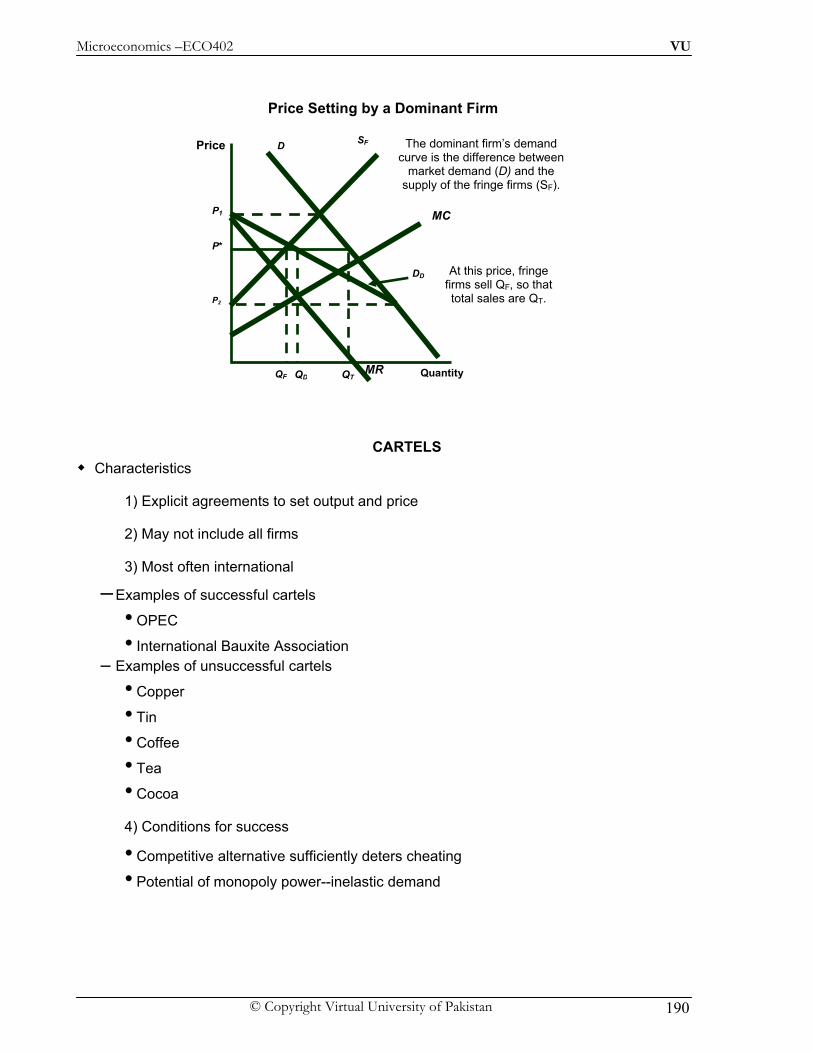
Microeconomics –ECO402 VU
© Copyright Virtual University of Pakistan 190
Price Setting by a Dominant Firm
CARTELS Characteristics
1) Explicit agreements to set output and price
2) May not include all firms
3) Most often international
– Examples of successful cartels
• OPEC
• International Bauxite Association – Examples of unsuccessful cartels
• Copper
• Tin
• Coffee
• Tea
• Cocoa
4) Conditions for success
• Competitive alternative sufficiently deters cheating
• Potential of monopoly power--inelastic demand
Price
Quantity
D
DD
QD
P*
At this price, fringe firms sell QF, so that total sales are QT.
P1
QF QT
P2
MC
MR
SF The dominant firm’s demand curve is the difference between
market demand (D) and the supply of the fringe firms (SF).
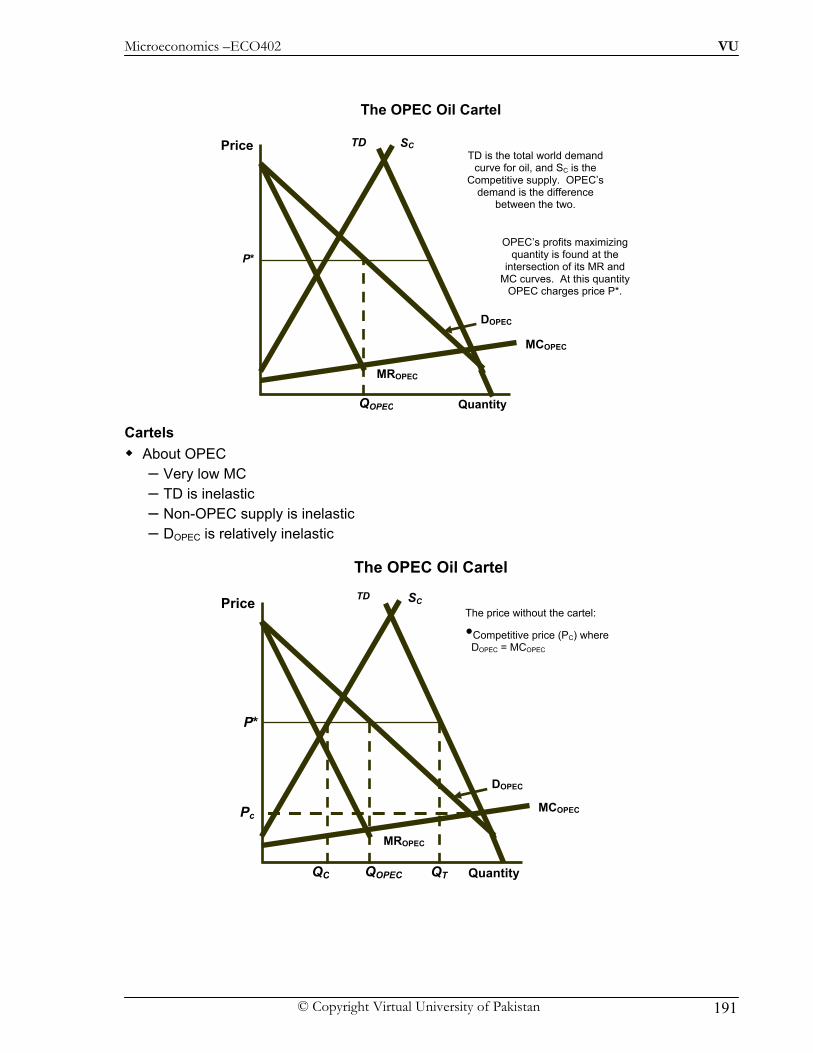
Microeconomics –ECO402 VU
© Copyright Virtual University of Pakistan 191
The OPEC Oil Cartel
Cartels About OPEC
– Very low MC – TD is inelastic – Non-OPEC supply is inelastic – DOPEC is relatively inelastic
The OPEC Oil Cartel
Price
Quantity
MROPEC
DOPEC
TD SC
MCOPEC
TD is the total world demand curve for oil, and SC is the
Competitive supply. OPEC’s demand is the difference
between the two.
QOPEC
P* OPEC’s profits maximizing
quantity is found at the intersection of its MR and
MC curves. At this quantity OPEC charges price P*.
Price
Quantity
MROPEC
DOPEC
TD SC
MCOPEC
QOPEC
P*
The price without the cartel:
•Competitive price (PC) where DOPEC = MCOPEC
QC QT
Pc
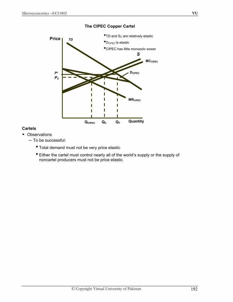
Microeconomics –ECO402 VU
© Copyright Virtual University of Pakistan 192
The CIPEC Copper Cartel
Cartels Observations
– To be successful:
• Total demand must not be very price elastic
• Either the cartel must control nearly all of the world’s supply or the supply of noncartel producers must not be price elastic.
Price
Quantity
MRCIPEC
TD
DCIPEC
SMCCIPEC
QCIPEC
P* PC
QC QT
•TD and SC are relatively elastic
•DCIPEC is elastic
•CIPEC has little monopoly power
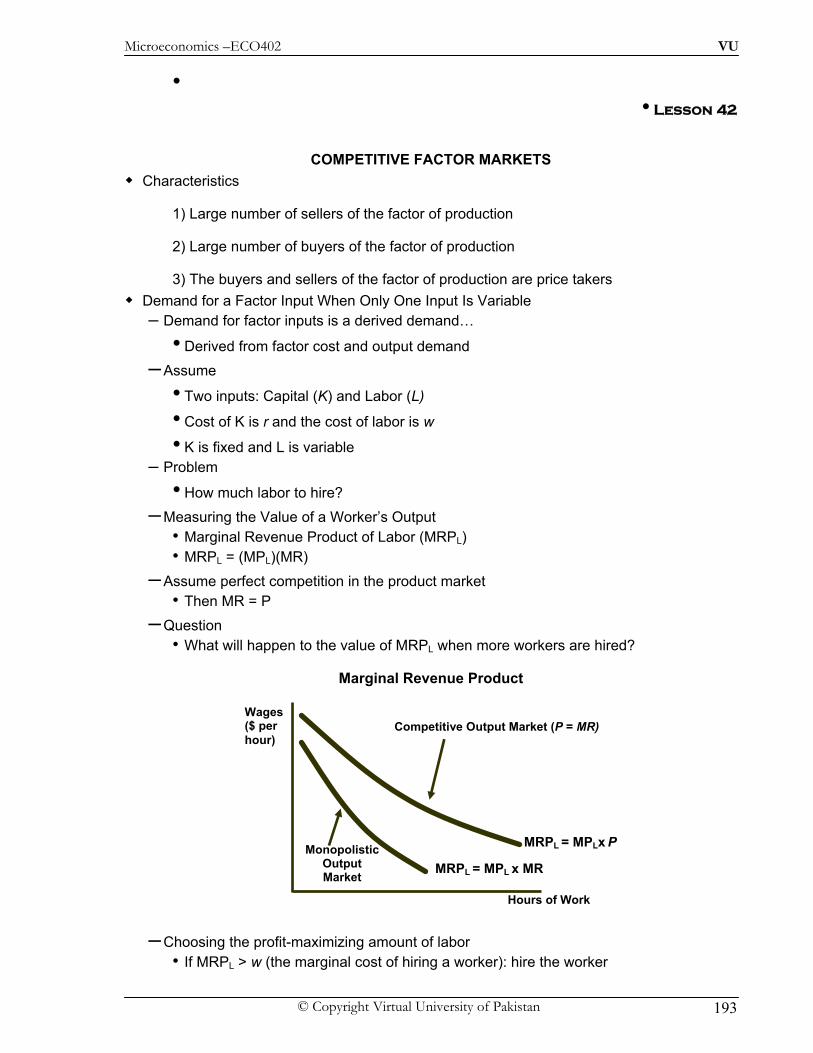
Microeconomics –ECO402 VU
© Copyright Virtual University of Pakistan 193
• • Lesson 42
COMPETITIVE FACTOR MARKETS Characteristics
1) Large number of sellers of the factor of production
2) Large number of buyers of the factor of production
3) The buyers and sellers of the factor of production are price takers Demand for a Factor Input When Only One Input Is Variable
– Demand for factor inputs is a derived demand…
• Derived from factor cost and output demand – Assume
• Two inputs: Capital (K) and Labor (L)
• Cost of K is r and the cost of labor is w
• K is fixed and L is variable – Problem
• How much labor to hire? – Measuring the Value of a Worker’s Output
• Marginal Revenue Product of Labor (MRPL) • MRPL = (MPL)(MR)
– Assume perfect competition in the product market • Then MR = P
– Question • What will happen to the value of MRPL when more workers are hired?
Marginal Revenue Product
– Choosing the profit-maximizing amount of labor • If MRPL > w (the marginal cost of hiring a worker): hire the worker
Hours of Work
Wages ($ per hour)
MRPL = MPLx P
Competitive Output Market (P = MR)
MRPL = MPL x MRMonopolistic
Output Market

Microeconomics –ECO402 VU
© Copyright Virtual University of Pakistan 194
• If MRPL < w: hire less labor • If MRPL = w: profit maximizing amount of labor
Hiring by a Firm in the Labor Market (with Capital Fixed)
Competitive Factor Markets Demand for a Factor Input When Only One Input Is Variable
– If the market supply of labor increased relative to demand (baby boomers or female entry), a surplus of labor would exist and the wage rate would fall.
– Question • How would this impact the quantity demanded for labor?
A Shift in the Supply of Labor
w S
In a competitive labor market, a firm faces a perfectly elastic supply of labor
and can hire as many workers as it wants at w*.
Quantity of Labor
Price of
Labor
Why not hire fewer or more workers than L*.
MRPL =
L
The profit maximizing firm will hire L* units of labor at the point
where the marginal revenue product of labor is equal to the wage rate.
Quantity of Labor
Price of Labor
w1 S1
MRPL = DL
L1
w2
L2
S2
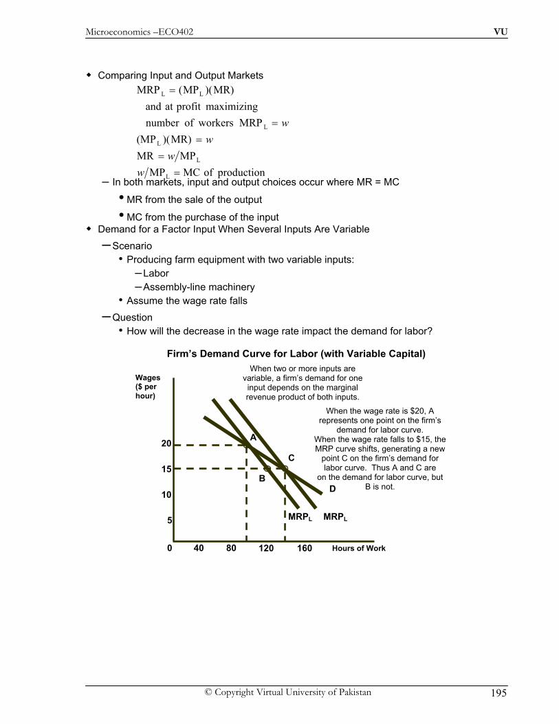
Microeconomics –ECO402 VU
© Copyright Virtual University of Pakistan 195
Comparing Input and Output Markets
– In both markets, input and output choices occur where MR = MC
• MR from the sale of the output
• MC from the purchase of the input Demand for a Factor Input When Several Inputs Are Variable
– Scenario • Producing farm equipment with two variable inputs:
– Labor – Assembly-line machinery
• Assume the wage rate falls
– Question • How will the decrease in the wage rate impact the demand for labor?
Firm’s Demand Curve for Labor (with Variable Capital)
production of MC MPMP MR
MR))((MPMRP workersofnumber
maximizingprofit at and MR))(MP(MRP
L
L
L
L
LL
==
==
=
ww
ww
MRPL MRPL
When two or more inputs are variable, a firm’s demand for one input depends on the marginal revenue product of both inputs.
Hours of Work
Wages ($ per hour)
0
5
10
15
20
40 80 120 160
When the wage rate is $20, A represents one point on the firm’s
demand for labor curve. When the wage rate falls to $15, the MRP curve shifts, generating a new
point C on the firm’s demand for labor curve. Thus A and C are
on the demand for labor curve, but B is not. D
A
B
C

Microeconomics –ECO402 VU
© Copyright Virtual University of Pakistan 196
Lesson 43
Competitive Factor Markets Industry Demand for Labor
– Assume that all firms respond to a lower wage • All firms would hire more workers. • Market supply would increase. • The market price will fall. • The quantity demanded for labor by the firm will be smaller.
The Industry Demand for Labor
Question – How would a change to a non-competitive market impact the derivation of the market
demand for labor?
The Demand for Jet Fuel Observations
– Jet fuel is a factor (input) cost – Cost of jet fuel
• 1971--Jet fuel cost equaled 12.4% of total operating cost
• 1980--Jet fuel cost equaled 30.0% of total operating cost
• 1990’s--Jet fuel cost equaled 15.0% of total operating cost – The demand for jet fuel impacts the airlines and refineries alike – The short-run price elasticity of demand for jet-fuel is very inelastic
Question – How would the long-run price elasticity of demand compare to the short-run?
12
MRPL
L
Industry Demand
Curve DL
MRPL
Labor(worker-hours)
Labor (worker-hours)
Wage ($ per hour)
Wage($ perhour)
0
5
10
15
0
5
10
15
50 100 150 L0 L
DL
Horizontal sum if product price unchanged
Firm Industry

Microeconomics –ECO402 VU
© Copyright Virtual University of Pakistan 197
The Short- and Long-Run
The Supply of Inputs to a Firm – Determining how much of an input to purchase
• Assume a perfectly competitive factor market
A Firm’s Input Supply in a Competitive Factor Market
The Market Supply of Inputs – The market supply for physical inputs is upward sloping
• Examples: jet fuel, fabric, steel – The market supply for labor may be upward sloping and backward bending
The Supply of Labor – The choice to supply labor is based on utility maximization – Leisure competes with labor for utility – Wage rate measures the price of leisure – Higher wage rate causes the price of leisure to increase
Quantity of Jet Fuel
Price
MRPLR MRPSR
SMarket Supplyof fabric
Yards ofFabric (thousands)
Yards ofFabric (thousands)
Price ($ per yard)
Price ($ per yard)
D
Market Demand
100
ME = AE10 10
Supply of Fabric Facing
50
Demand for Fabric
MRP
Observations 1) The firm is a price taker at $10. 2) S = AE = ME = $10 3) ME = MRP @ 50 units

Microeconomics –ECO402 VU
© Copyright Virtual University of Pakistan 198
– Higher wages encourage workers to substitute work for leisure (i.e. the substitution effect)
– Higher wages allow the worker to purchase more goods, including leisure which reduces work hours (i.e. the income effect)
– If the income effect exceeds the substitution effect the supply curve is backward bending
Backward-Bending Supply of Labor
Substitution and Income Effects of a Wage Increase
Income Effect <Substitution Effect
Income Effect >Substitution Effect
Hours of Work per Day
Wage ($ per hour)
Supply of Labor
12
C
Worker chooses point A:
•16 hours leisure, 8 hour work
16Q
P
A
w = $10
Hours of Leisure
Income ($ per
day)
0
240
8 24
480
20
B
w = $20
Suppose wages increase to $20
Substitution effect Income effect
Increase wage to $20 worker chooses: 20 hour leisure, 4 hours work income = $80
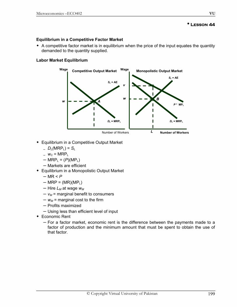
Microeconomics –ECO402 VU
© Copyright Virtual University of Pakistan 199
• Lesson 44
Equilibrium in a Competitive Factor Market A competitive factor market is in equilibrium when the price of the input equates the quantity
demanded to the quantity supplied.
Labor Market Equilibrium
Equilibrium in a Competitive Output Market – DL(MRPL) = SL
– wC = MRPL
– MRPL = (P)(MPL) – Markets are efficient
Equilibrium in a Monopolistic Output Market – MR < P – MRP = (MR)(MPL) – Hire LM at wage wM – vM = marginal benefit to consumers – wM = marginal cost to the firm – Profits maximized – Using less than efficient level of input
Economic Rent – For a factor market, economic rent is the difference between the payments made to a
factor of production and the minimum amount that must be spent to obtain the use of that factor.
SL = AE SL = AE
DL = MRPL DL = MRPL
P * MPL
Number of Workers Number of Workers
Wage WageCompetitive Output Market Monopolistic Output Market
w
L
w
L
v
A B

Microeconomics –ECO402 VU
© Copyright Virtual University of Pakistan 200
Question – What would be the economic rent if SL is perfectly elastic or perfectly inelastic?
Land: A Perfectly Inelastic Supply – With land inelastically supplied, its price is determined entirely by demand, at least in the
short run.
Land Rent Pay in the Public Sector
The percentage of personnel working in public sector has been declining Shortages of skilled personnel has occurred? Why?
– If there is a shortage, the wage must be below the competitive wage rate
The Shortage of Skilled Personnel
Number of Acres
Price ($ per acre)
Supply of Land
D2
EconomicRent
s2
D1
EconomicRent
s1
Number of Skilled Workers
Wage S
DL =
w*
wShortage
Total expenditure (wage) paid is 0w* x AL* Economic Rent
Economic rent is ABW*
B
Number of Workers
Wage
SL = AE
DL = MRPL
w*
L*
A
0
The economic rent associated with the employment of labor is the excess of wages
paid above the minimum amount needed to hire workers.
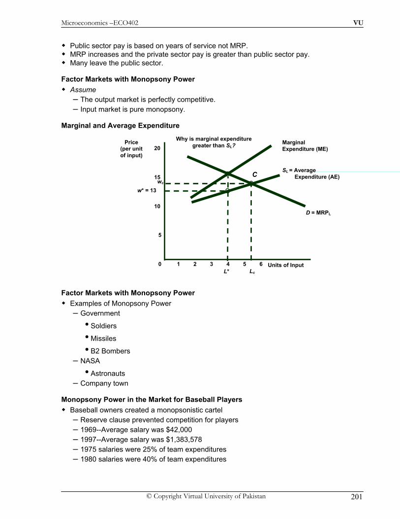
Microeconomics –ECO402 VU
© Copyright Virtual University of Pakistan 201
Public sector pay is based on years of service not MRP. MRP increases and the private sector pay is greater than public sector pay. Many leave the public sector.
Factor Markets with Monopsony Power Assume
– The output market is perfectly competitive. – Input market is pure monopsony.
Marginal and Average Expenditure
Factor Markets with Monopsony Power Examples of Monopsony Power
– Government
• Soldiers
• Missiles
• B2 Bombers – NASA
• Astronauts – Company town
Monopsony Power in the Market for Baseball Players Baseball owners created a monopsonistic cartel
– Reserve clause prevented competition for players – 1969--Average salary was $42,000 – 1997--Average salary was $1,383,578 – 1975 salaries were 25% of team expenditures – 1980 salaries were 40% of team expenditures
SL = Average Expenditure (AE)
Marginal Expenditure (ME)
Why is marginal expendituregreater than SL?
D = MRPL
Units of Input
Price (per unit of input)
0 1 2 3 4 65
5
10
15
20
w* = 13
L*
wc
Lc
C

Microeconomics –ECO402 VU
© Copyright Virtual University of Pakistan 202
–
Lesson 45
Factor Markets with Monopoly Power Just as buyers of inputs can have monopsony power, sellers of inputs can have monopoly
power. The most important example of monopoly power in factor markets involves labor unions.
Monopoly Power of Sellers of Labor
Monopoly Power of Sellers of Labor
The primary determinant of controlling wage and economic rent is controlling the supply of labor
A Two-Sector Model of Labor Employment – Union monopoly power impacts the nonunionized part of the economy.
SL
DL
MR
When a labor union is a monopolist, it chooses among points on the buyer’s
demand for labor curve.
Number of Workers
Wage per
worker
A
L*
w*
The seller can maximize the number of workers hired, at L*, by agreeing that
workers will work at wage w*.
Economic Rent
w1
L1
The quantity of labor L1 that maximizes the rent that employees earn is determined by the intersection of the marginal revenue and supply or labor curves; union members receive a wage rate of w1.
SL
DL
MR
Number of Workers
Wage per
worker
A
L2
w2
Finally, if the union wishes to maximize total wages paid to workers, it should allow L2 union members to be employed at a wage rate of w2 because the orginal revenue to the union will then be zero.
L*
w*
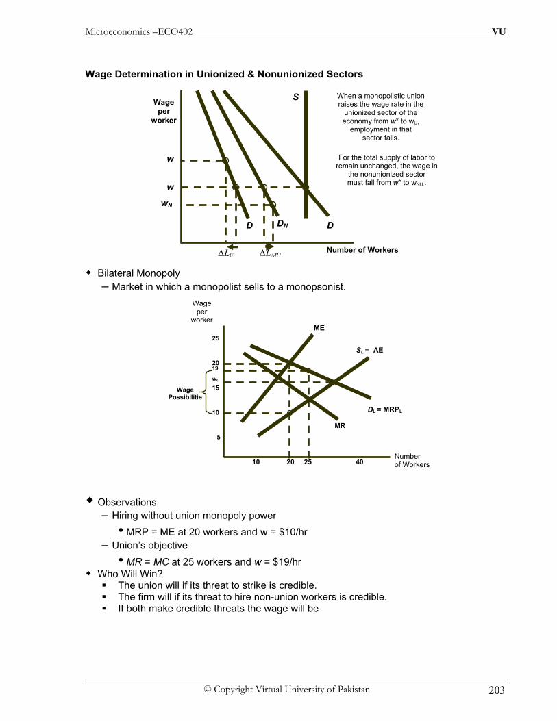
Microeconomics –ECO402 VU
© Copyright Virtual University of Pakistan 203
Wage Determination in Unionized & Nonunionized Sectors
Bilateral Monopoly – Market in which a monopolist sells to a monopsonist.
Observations – Hiring without union monopoly power
• MRP = ME at 20 workers and w = $10/hr – Union’s objective
• MR = MC at 25 workers and w = $19/hr Who Will Win?
The union will if its threat to strike is credible. The firm will if its threat to hire non-union workers is credible. If both make credible threats the wage will be
Number of Workers
Wage per
worker
D DN D
S
w
w
When a monopolistic union raises the wage rate in the
unionized sector of the economy from w* to wU,
employment in that sector falls.
ΔLU
For the total supply of labor to remain unchanged, the wage in
the nonunionized sector must fall from w* to wNU..
wN
ΔLMU
Number of Workers
Wage per
worker
DL = MRPL
MR5
10
15
20
25
10 20 40
SL = AE
ME
25
19
Wage Possibilitie
wC