1

Efficient Almost Wait-freeParallel Accessible Dynamic Hashtables

Gao, H.1, Groote, J.F.2, Hesselink, W.H.11 Department of Mathematics and Computing Science, University of Groningen, P.O. Box 800, 9700 AV

Groningen, The Netherlands(Email: {hui,wim}@cs.rug.nl)2 Department of Mathematics and Computing Science, Eindhoven University of Technology, P.O. Box

513, 5600 MB Eindhoven, The Netherlands and CWI, P.O. Box 94079, 1090 GB Amsterdam, The

Netherlands (Email: jfg@win.tue.nl)

Abstract

In multiprogrammed systems, synchronization often turns out to be a performance bottleneckand the source of poor fault-tolerance. Wait-free and lock-free algorithms can do withoutlocking mechanisms, and therefore do not suffer from these problems. We present an efficientalmost wait-free algorithm for parallel accessible hashtables, which promises more robustperformance and reliability than conventional lock-based implementations. Our solution is asefficient as sequential hashtables. It can easily be implemented using C-like languages andrequires on average only constant time for insertion, deletion or accessing of elements. Apartfrom that, our new algorithm allows the hashtables to grow and shrink dynamically whenneeded.

A true problem of lock-free algorithms is that they are hard to design correctly, even whenapparently straightforward. Ensuring the correctness of the design at the earliest possiblestage is a major challenge in any responsible system development. Our algorithm contains81 atomic statements. In view of the complexity of the algorithm and its correctness prop-erties, we turned to the interactive theorem prover PVS for mechanical support. We employstandard deductive verification techniques to prove around 200 invariance properties of ouralmost wait-free algorithm, and describe how this is achieved using the theorem prover PVS.

CR Subject Classification (1991): D.1 Programming techniquesAMS Subject Classification (1991): 68Q22 Distributed algorithms, 68P20 Information storageand retrievalKeywords & Phrases: Hashtables, Distributed algorithms, Lock-free, Wait-free

1 Introduction

We are interested in efficient, reliable, parallel algorithms. The classical synchronization paradigmsare not most suited for this, because synchronization often turns out a performance bottleneck,and failure of a single process can force all other processes to come to a halt. Therefore, wait-free,lock-free, or synchronization-free algorithms are of interest [11, 19, 13].

An algorithm is wait-free when each process can accomplish its task in a finite number ofsteps, independently of the activity and speed of other processes. An algorithm is lock-free whenit guarantees that within a finite number of steps always some process will complete its tasks, evenif other processes halt. An algorithm is synchronization-free when it does not contain synchroniza-tion primitives. The difference between wait-free and lock-free is that a lock-free process can bearbitrarily delayed by other processes that repeatedly start and accomplish tasks. The differencebetween synchronization-free and lock-free is that in a synchronization-free algorithm processesmay delay each other arbitrarily, without getting closer to accomplishing their respective tasks.As we present a lock-free algorithm, we only speak about lock-freedom below, but most applies towait-freedom or synchronization-freedom as well.

Since the processes in a lock-free algorithm run rather independently of each other, lock-freealgorithms scale up well when there are more processes. Processors can finish their tasks on theirown, without being blocked, and generally even without being delayed by other processes. So,there is no need to wait for slow or overloaded processors. In fact, when there are processors of

2

differing speeds, or under different loads, a lock-free algorithm will generally distribute commontasks over all processors, such that it is finished as quickly as possible.

As argued in [13], another strong argument for lock-free algorithms is reliability. A lock-freealgorithm will carry out its task even when all but one processor stops working. Without problemit can stand any pattern of processors being switched off and on again. The only noticeable effectof failing processors is that common tasks will be carried out somewhat slower, and the failingprocessor may have claimed resources, such as memory, that it can not relinquish anymore.

For many algorithms the penalty to be paid is minor; setting some extra control variables, or us-ing a few extra pointer indirections suffices. Sometimes, however, the time and space complexitiesof a lock-free algorithm is substantially higher than its sequential, or ‘synchronized’ counterpart[7]. Furthermore, some machine architectures are not very capable of handling shared variables,and do not offer compare-and-swap or test-and-set instructions necessary to implement lock-freealgorithms.

Hashtables are very commonly in use to efficiently store huge but sparsely filled tables. Asfar as we know, no wait- or lock-free algorithm for hashtables has ever been proposed. There arevery general solutions for wait-free addresses in general [1, 2, 6, 9, 10], but these are not efficient.Furthermore, there exist wait-free algorithms for different domains, such as linked lists [19], queues[20] and memory management [8, 11]. In this paper we present an almost wait-free algorithm forhashtables. Strictly speaking, the algorithm is only lock-free, but wait-freedom is only violatedwhen a hashtable is resized, which is a relatively rare operation. We allow fully parallel insertion,deletion and finding of elements. As a correctness notion, we take that the operations behavethe same as for ‘ordinary’ hashtables, under some arbitrary serialization of these operations. So,if a find is carried out strictly after an insert, the inserted element is found. If insert and findare carried out at the same time, it may be that find takes place before insertion, and it is notdetermined whether an element will be returned.

An important feature of our hashtable is that it can dynamically grow and shrink when needed.This requires subtle provisions, which can be best understood by considering the following scenar-ios. Suppose that process A is about to (slowly) insert an element in a hashtable H1. Before thishappens, however, a fast process B has resized the hashtable by making a new hashtable H2, andhas copied the content from H1 to H2. If (and only if) process B did not copy the insertion of A,A must be informed to move to the new hashtable, and carry out the insertion there. Suppose aprocess C comes into play also copying the content from H1 to H2. This must be possible, sinceotherwise B can stop copying, blocking all operations of other processes on the hashtable, andthus violating the lock-free nature of the algorithm. Now the value inserted by A can but need notbe copied by both B and/or C. This can be made more complex by a process D that attemptsto replace H2 by H3. Still, the value inserted by A should show up exactly once in the hashtable,and it is clear that processes should carefully keep each other informed about their activities onthe tables.

A true problem of lock-free algorithms is that they are hard to design correctly, which evenholds for apparently straightforward algorithms. Whereas human imagination generally suffices todeal with all possibilities of sequential processes or synchronized parallel processes, this appearsimpossible (at least to us) for lock-free algorithms. The only technique that we see fit for any butthe simplest lock-free algorithms is to prove the correctness of the algorithm very precisely, andto double check this using a proof checker or theorem prover.

Our algorithm contains 81 atomic statements. The structure of our algorithm and its correct-ness properties, as well as the complexity of reasoning about them, makes neither automatic normanual verification feasible. We have therefore chosen the higher-order interactive theorem proverPVS [3, 18] for mechanical support. PVS has a convenient specification language and contains aproof checker which allows users to construct proofs interactively, to automatically execute trivialproofs, and to check these proofs mechanically.

Our solution is as efficient as sequential hashtables. It requires on average only constant timefor insertion, deletion or accessing of elements.

3

Overview of the paper

Section 2 contains the description of the hashtable interface offered to the users. The algorithmis presented in Section 3. Section 4 contains a description of the proof of the safety properties ofthe algorithm: functional correctness, atomicity, and absence of memory loss. This proof is basedon a list of around 200 invariants, presented in Appendix A, while the relationships between theinvariants are given by a dependency graph in Appendix B. Progress of the algorithm is provedinformally in Section 5. Conclusions are drawn in Section 6.

2 The interface

The aim is to construct a hashtable that can be accessed simultaneously by different processes insuch a way that no process can passively block another process’ access to the table.

A hashtable is an implementation of (partial) functions between two domains, here calledAddress and Value. The hashtable thus implements a modifiable shared variable X ∈ Address →Value. The domains Address and Value both contain special default elements 0 ∈ Address andnull ∈ Value. An equality X(a) = null means that no value is currently associated with theaddress a. In particular, since we never store a value for the address 0, we impose the invariant

X(0) = null .

We use open addressing to keep all elements within the table. For the implementation of thehashtables we require that from every value the address it corresponds to is derivable. We thereforeassume that some function ADR ∈ Value → Address is given with the property that

Ax1: v = null ≡ ADR(v) = 0

Indeed, we need null as the value corresponding to the undefined addresses and use address 0 asthe (only) address associated with the value null. We thus require the hashtable to satisfy theinvariant

X(a) 6= null ⇒ ADR(X(a)) = a .

Note that the existence of ADR is not a real restriction since one can choose to store the pair (a, v)instead of v. When a can be derived from v, it is preferable to store v, since that saves memory.

There are four principle operations: find, delete, insert and assign. The first one is to find thevalue currently associated with a given address. This operation yields null if the address has noassociated value. The second operation is to delete the value currently associated with a givenaddress. It fails if the address was empty, i.e. X(a) = null. The third operation is to insert a newvalue for a given address, provided the address was empty. So, note that at least one out of twoconsecutive inserts for address a must fail, except when there is a delete for address a in betweenthem. The operation assign does the same as insert, except that it rewrites the value even if theassociated address is not empty. Moreover, assign never fails.

We assume that there is a bounded number of processes that may need to interact with thehashtable. Each process is characterized by the sequence of operations

( getAccess ; (find + delete + insert + assign)∗ ; releaseAccess)ω

A process that needs to access the table, first calls the procedure getAccess to get the currenthashtable pointer. It may then invoke the procedures find, delete, insert, and assign repeatedly,in an arbitrary, serial manner. A process that has access to the table can call releaseAccess tolog out. The processes may call these procedures concurrently. The only restriction is that everyprocess can do at most one invocation at a time.

The basic correctness conditions for concurrent systems are functional correctness and atom-icity, say in the sense of [16], Chapter 13. Functional correctness is expressed by prescribing howthe procedures find, insert, delete, assign affect the value of the abstract mapping X. Atomicity isexpressed by the condition that the modification of X is executed atomically at some time between

4

the invocation of the routine and its response. Each of these procedures has the precondition thatthe calling process has access to the table. In this specification, we use auxiliary private variablesdeclared locally in the usual way. We give them the suffix S to indicate that the routines below arethe specifications of the procedures. We use angular brackets 〈 and 〉 to indicate atomic executionof the enclosed command.

proc findS(a : Address \ {0}) : Value =local rS : Value;

(fS) 〈 rS := X(a) 〉;return rS.

proc deleteS(a : Address \ {0}) : Bool =local sucS : Bool;

(dS) 〈 sucS := (X[a] 6= null) ;if sucS then X[a] := null end 〉 ;

return sucS.

proc insertS(v : Value \ {null}) : Bool =local sucS : Bool ; a : Address := ADR(v) ;

(iS) 〈 sucS := (X[a] = null) ;if sucS then X[a] := v end 〉 ;

return sucS.

proc assignS(v : Value \ {null}) =local a : Address := ADR(v) ;

(aS) 〈 X[a] := v 〉 ;end.

Note that, in all cases, we require that the body of the procedure is executed atomically at somemoment between the beginning and the end of the call, but that this moment need not coincidewith the beginning or end of the call. This is the reason that we do not (e.g.) specify find by thesingle line return X(a).

Due to the parallel nature of our system we cannot use pre and postconditions to specify it.For example, it may happen that insert(v) returns true while X(ADR(v)) = null since anotherprocess deletes ADR(v) between the execution of (iS) and the response of insert.

We prove partial correctness by extending the implementation with the auxiliary variables andcommands used in the specification. So, we regard X as a shared auxiliary variable and rS andsucS as private auxiliary variables; we augment the implementations of find, delete, insert, assignwith the atomic commands (fS), (dS), (iS), (aS), respectively. We prove that the implementationof the procedure below executes its atomic specification command always precisely once and thatthe resulting value r or suc of the implementation equals the resulting value rS or sucS in thespecification above. It follows that, by removing the implementation variables from the combinedprogram, we obtain the specification. This removal may eliminate many atomic steps of theimplementation. This is known as removal of stutterings in TLA [14] or abstraction from τ stepsin process algebras.

3 The algorithm

An implementation consists of P processes along with a set of variables, for P ≥ 1. Each process,numbered from 1 up to P , is a sequential program comprised of atomic statements. Actions onprivate variables can be added to an atomic statement, but all actions on shared variables mustbe separated into atomic accesses. Since auxiliary variables are only used to facilitate the proof ofcorrectness, they can be assumed to be touched instantaneously without violation of the atomicityrestriction.

5

3.1 Hashing

We implement function X via hashing with open addressing, cf. [15, 21]. We do not use directchaining, where colliding entries are stored in a secondary list, because maintaining these listsin a lock-free manner is tedious [19], and expensive when done wait-free. A disadvantage ofopen addressing with deletion of elements is that the contents of the hashtable must regularly berefreshed by copying the non-deleted elements to a new hashtable. As we wanted to be able toresize the hashtables anyhow, we consider this less of a burden.

In principle, hashing is a way to store address-value pairs in an array (hashtable) with a lengthmuch smaller than the number of potential addresses. The indices of the array are determinedby a hash function. In case the hash function maps two addresses to the same index in the arraythere must be some method to determine an alternative index. The question how to choose agood hash function and how to find alternative locations in the case of open addressing is treatedextensively elsewhere, e.g. [15].

For our purposes it is convenient to combine these two roles in one abstract function key givenby:

key(a : Address, l : Nat, n : Nat) : Nat ,

where l is the length of the array (hashtable), that satisfies

Ax2: 0 ≤ key(a, l, n) < l

for all a, l, and n. The number n serves to obtain alternative locations in case of collisions: whenthere is a collision, we re-hash until an empty “slot” (i.e. null) or the same address in the tableis found. The approach with a third argument n is unusual but very general. It is more usual tohave a function Key dependent on a and l, and use a second function Inc, which may depend ona and l, to use in case of collisions. Then our function key is obtained recursively by

key(a, l, 0) = Key(a, l) and key(a, l, n+ 1) = Inc(a, l, key(a, l, n)) .

We require that, for any address a and any number l, the first l keys are all different, as expressedin

Ax3: 0 ≤ k < m < l ⇒ key(a, l, k) 6= key(a, l,m) .

3.2 Tagging of values

In hashtables with open addressing a deleted value cannot be replaced by null since null signalsthe end of the search. Therefore, such a replacement would invalidate searches for other values.Instead, we introduce an additional “value” del to replace deleted values.

Since we want the values in the hashtable to migrate to a bigger table when the first tablebecomes full, we need to tag values that are being migrated. We cannot simply remove such avalue from the old table, since the migrating process may stop functioning during the migration.Therefore, a value being copied must be tagged in such a way that it is still recognizable. This isdone by the function old. We thus introduce an extended domain of values to be called EValue,which is defined as follows:

EValue = {del} ∪Value ∪ {old(v) | v ∈ Value}

We furthermore assume the existence of functions val : EValue → Value and oldp : EValue → Boolthat satisfy, for all v ∈ Value:

val(v) = vval(del) = nullval(old(v)) = voldp(v) = falseoldp(del) = falseoldp(old(v)) = true

6

Note that the old tag can easily be implemented by designating one special bit in the representationof Value. In the sequel we write done for old(null). Moreover, we extend the function ADR todomain EValue by ADR(v) = ADR(val(v)).

3.3 Data structure

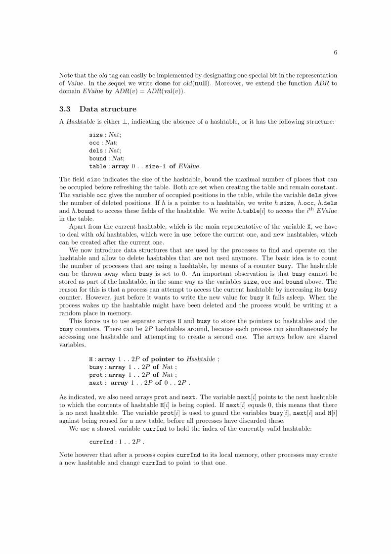
A Hashtable is either ⊥, indicating the absence of a hashtable, or it has the following structure:

size : Nat;occ : Nat;dels : Nat;bound : Nat;table : array 0 . . size-1 of EValue.

The field size indicates the size of the hashtable, bound the maximal number of places that canbe occupied before refreshing the table. Both are set when creating the table and remain constant.The variable occ gives the number of occupied positions in the table, while the variable dels givesthe number of deleted positions. If h is a pointer to a hashtable, we write h.size, h.occ, h.delsand h.bound to access these fields of the hashtable. We write h.table[i] to access the ith EValuein the table.

Apart from the current hashtable, which is the main representative of the variable X, we haveto deal with old hashtables, which were in use before the current one, and new hashtables, whichcan be created after the current one.

We now introduce data structures that are used by the processes to find and operate on thehashtable and allow to delete hashtables that are not used anymore. The basic idea is to countthe number of processes that are using a hashtable, by means of a counter busy. The hashtablecan be thrown away when busy is set to 0. An important observation is that busy cannot bestored as part of the hashtable, in the same way as the variables size, occ and bound above. Thereason for this is that a process can attempt to access the current hashtable by increasing its busycounter. However, just before it wants to write the new value for busy it falls asleep. When theprocess wakes up the hashtable might have been deleted and the process would be writing at arandom place in memory.

This forces us to use separate arrays H and busy to store the pointers to hashtables and thebusy counters. There can be 2P hashtables around, because each process can simultaneously beaccessing one hashtable and attempting to create a second one. The arrays below are sharedvariables.

H : array 1 . . 2P of pointer to Hashtable ;busy : array 1 . . 2P of Nat ;prot : array 1 . . 2P of Nat ;next : array 1 . . 2P of 0 . . 2P .

As indicated, we also need arrays prot and next. The variable next[i] points to the next hashtableto which the contents of hashtable H[i] is being copied. If next[i] equals 0, this means that thereis no next hashtable. The variable prot[i] is used to guard the variables busy[i], next[i] and H[i]against being reused for a new table, before all processes have discarded these.

We use a shared variable currInd to hold the index of the currently valid hashtable:

currInd : 1 . . 2P .

Note however that after a process copies currInd to its local memory, other processes may createa new hashtable and change currInd to point to that one.

7

3.4 Primary procedures

We first provide the code for the primary procedures, which match directly with the proceduresin the interface. Every process has a private variable

index : 1 . . 2P ;

containing what it regards as the currently active hashtable. At entry of each primary procedure,it must be the case that the variable H[index] contains valid information. In section 3.5, we provideprocedure getAccess with the main purpose to guarantee this property. When getAccess has beencalled, the system is obliged to keep the hashtable at index stored in memory, even if there areno accesses to the hashtable using any of the primary procedures. A procedure releaseAccess isprovided to release resources, and it should be called whenever the process will not access thehashtable for some time.

3.4.1 Syntax

We use a syntax analogous to Modula-3 [5]. We use := for the assignment. We use the C–operations ++ and -- for atomic increments and decrements. The semicolon is a separator, not aterminator. The basic control mechanisms are

loop .. end is an infinite loop, terminated by exit or returnwhile .. do .. end and repeat .. until .. are ordinary repetitionsif .. then .. {elsif ..} [else ..] end is the conditionalcase .. end is a case statement.

Types are slanted and start with a capital. Shared variables and shared data elements are intypewriter font. Private variables are slanted or in math italic.

3.4.2 The main loop

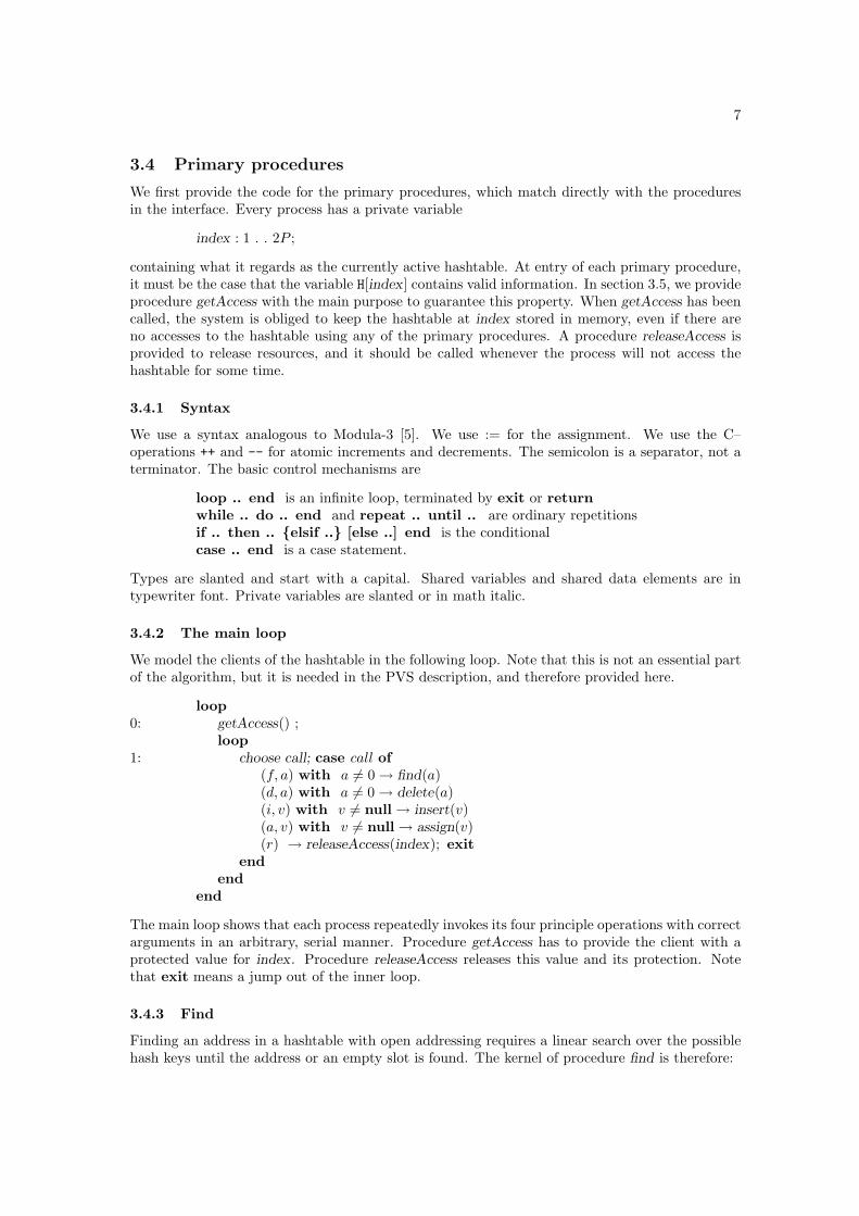
We model the clients of the hashtable in the following loop. Note that this is not an essential partof the algorithm, but it is needed in the PVS description, and therefore provided here.

loop0: getAccess() ;

loop1: choose call; case call of

(f, a) with a 6= 0 → find(a)(d, a) with a 6= 0 → delete(a)(i, v) with v 6= null → insert(v)(a, v) with v 6= null → assign(v)(r) → releaseAccess(index); exit

endend

end

The main loop shows that each process repeatedly invokes its four principle operations with correctarguments in an arbitrary, serial manner. Procedure getAccess has to provide the client with aprotected value for index. Procedure releaseAccess releases this value and its protection. Notethat exit means a jump out of the inner loop.

3.4.3 Find

Finding an address in a hashtable with open addressing requires a linear search over the possiblehash keys until the address or an empty slot is found. The kernel of procedure find is therefore:

8

n := 0 ;repeat r := h.table[key(a, l, n)] ; n++ ;until r = null ∨ a = ADR(r) ;

The main complication is that the process has to join the migration activity by calling refreshwhen it encounters an entry done (i.e. old(null)).

Apart from a number of special commands, we group statements such that at most one sharedvariable is accessed and label these ‘atomic’ statements with a number. The labels are chosenidentical to the labels in the PVS code, and therefore not completely consecutive.

In every execution step, one of the processes proceeds from one label to a next one. The stepsare thus treated as atomic. The atomicity of steps that refer to shared variables more than onceis emphasized by enclosing them in angular brackets. Since procedure calls only modify privatecontrol data, procedure headers are not always numbered themselves, but their bodies usuallyhave numbered atomic statements.

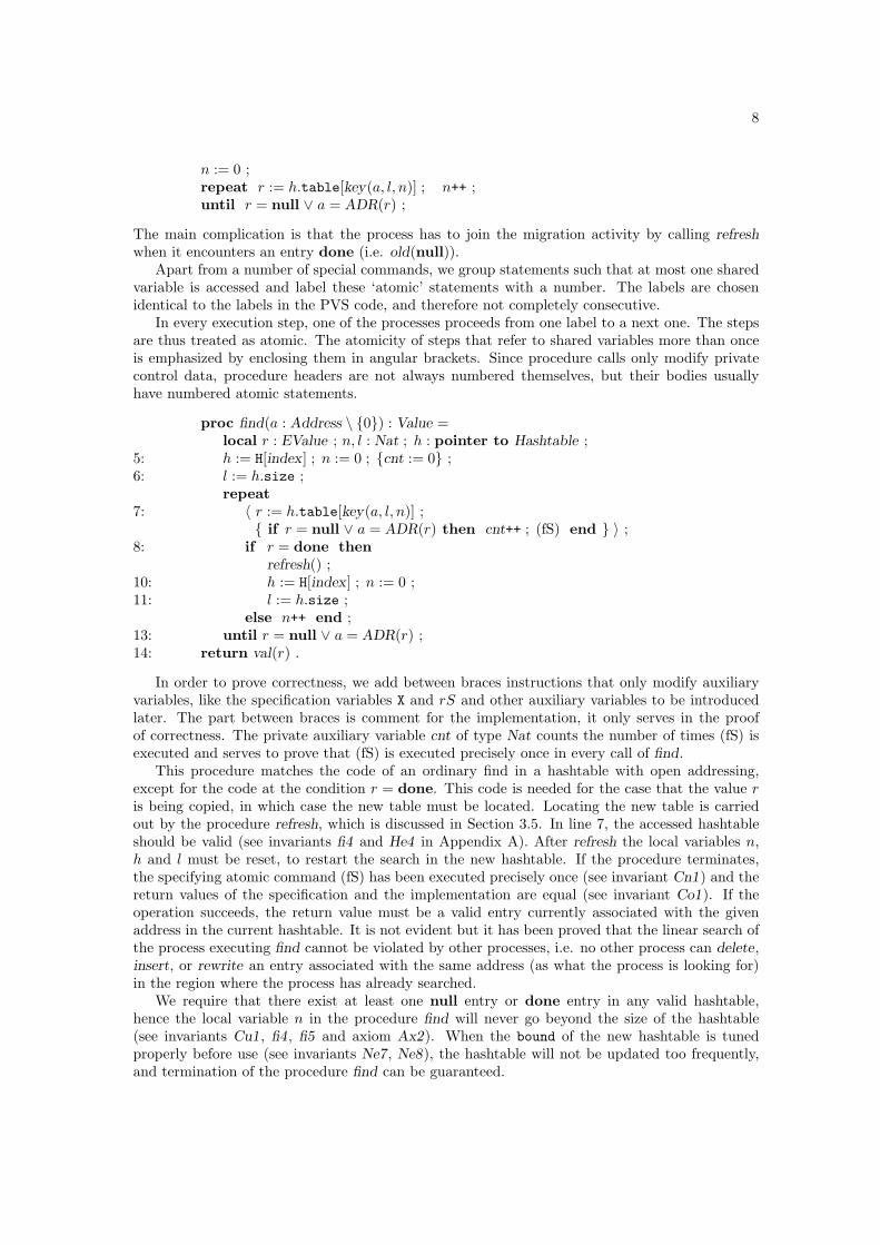
proc find(a : Address \ {0}) : Value =local r : EValue ; n, l : Nat ; h : pointer to Hashtable ;

5: h := H[index] ; n := 0 ; {cnt := 0} ;6: l := h.size ;

repeat7: 〈 r := h.table[key(a, l, n)] ;

{ if r = null ∨ a = ADR(r) then cnt++ ; (fS) end } 〉 ;8: if r = done then

refresh() ;10: h := H[index] ; n := 0 ;11: l := h.size ;

else n++ end ;13: until r = null ∨ a = ADR(r) ;14: return val(r) .

In order to prove correctness, we add between braces instructions that only modify auxiliaryvariables, like the specification variables X and rS and other auxiliary variables to be introducedlater. The part between braces is comment for the implementation, it only serves in the proofof correctness. The private auxiliary variable cnt of type Nat counts the number of times (fS) isexecuted and serves to prove that (fS) is executed precisely once in every call of find.

This procedure matches the code of an ordinary find in a hashtable with open addressing,except for the code at the condition r = done. This code is needed for the case that the value ris being copied, in which case the new table must be located. Locating the new table is carriedout by the procedure refresh, which is discussed in Section 3.5. In line 7, the accessed hashtableshould be valid (see invariants fi4 and He4 in Appendix A). After refresh the local variables n,h and l must be reset, to restart the search in the new hashtable. If the procedure terminates,the specifying atomic command (fS) has been executed precisely once (see invariant Cn1) and thereturn values of the specification and the implementation are equal (see invariant Co1). If theoperation succeeds, the return value must be a valid entry currently associated with the givenaddress in the current hashtable. It is not evident but it has been proved that the linear search ofthe process executing find cannot be violated by other processes, i.e. no other process can delete,insert, or rewrite an entry associated with the same address (as what the process is looking for)in the region where the process has already searched.

We require that there exist at least one null entry or done entry in any valid hashtable,hence the local variable n in the procedure find will never go beyond the size of the hashtable(see invariants Cu1, fi4, fi5 and axiom Ax2). When the bound of the new hashtable is tunedproperly before use (see invariants Ne7, Ne8), the hashtable will not be updated too frequently,and termination of the procedure find can be guaranteed.

9

3.4.4 Delete

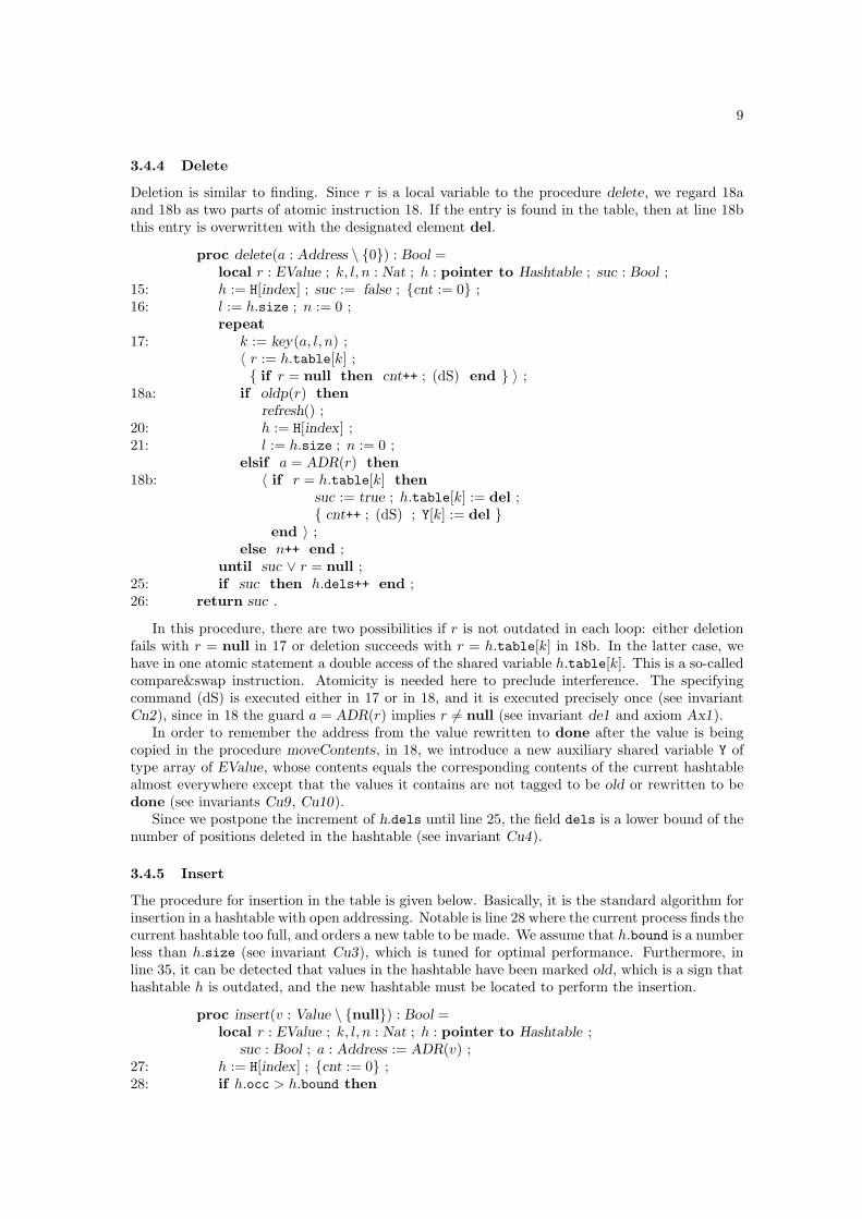
Deletion is similar to finding. Since r is a local variable to the procedure delete, we regard 18aand 18b as two parts of atomic instruction 18. If the entry is found in the table, then at line 18bthis entry is overwritten with the designated element del.

proc delete(a : Address \ {0}) : Bool =local r : EValue ; k, l, n : Nat ; h : pointer to Hashtable ; suc : Bool ;

15: h := H[index] ; suc := false ; {cnt := 0} ;16: l := h.size ; n := 0 ;

repeat17: k := key(a, l, n) ;

〈 r := h.table[k] ;{ if r = null then cnt++ ; (dS) end } 〉 ;

18a: if oldp(r) thenrefresh() ;

20: h := H[index] ;21: l := h.size ; n := 0 ;

elsif a = ADR(r) then18b: 〈 if r = h.table[k] then

suc := true ; h.table[k] := del ;{ cnt++ ; (dS) ; Y[k] := del }

end 〉 ;else n++ end ;

until suc ∨ r = null ;25: if suc then h.dels++ end ;26: return suc .

In this procedure, there are two possibilities if r is not outdated in each loop: either deletionfails with r = null in 17 or deletion succeeds with r = h.table[k] in 18b. In the latter case, wehave in one atomic statement a double access of the shared variable h.table[k]. This is a so-calledcompare&swap instruction. Atomicity is needed here to preclude interference. The specifyingcommand (dS) is executed either in 17 or in 18, and it is executed precisely once (see invariantCn2), since in 18 the guard a = ADR(r) implies r 6= null (see invariant de1 and axiom Ax1).

In order to remember the address from the value rewritten to done after the value is beingcopied in the procedure moveContents, in 18, we introduce a new auxiliary shared variable Y oftype array of EValue, whose contents equals the corresponding contents of the current hashtablealmost everywhere except that the values it contains are not tagged to be old or rewritten to bedone (see invariants Cu9, Cu10).

Since we postpone the increment of h.dels until line 25, the field dels is a lower bound of thenumber of positions deleted in the hashtable (see invariant Cu4).

3.4.5 Insert

The procedure for insertion in the table is given below. Basically, it is the standard algorithm forinsertion in a hashtable with open addressing. Notable is line 28 where the current process finds thecurrent hashtable too full, and orders a new table to be made. We assume that h.bound is a numberless than h.size (see invariant Cu3), which is tuned for optimal performance. Furthermore, inline 35, it can be detected that values in the hashtable have been marked old, which is a sign thathashtable h is outdated, and the new hashtable must be located to perform the insertion.

proc insert(v : Value \ {null}) : Bool =local r : EValue ; k, l, n : Nat ; h : pointer to Hashtable ;

suc : Bool ; a : Address := ADR(v) ;27: h := H[index] ; {cnt := 0} ;28: if h.occ > h.bound then

10

newTable() ;30: h := H[index] end ;31: n := 0 ; l := h.size ; suc := false ;

repeat32: k := key(a, l, n) ;33: 〈 r := h.table[k] ;

{ if a = ADR(r) then cnt++ ; (iS) end } 〉 ;35a: if oldp(r) then

refresh() ;36: h := H[index] ;37: n := 0 ; l := h.size ;

elseif r = null then35b: 〈 if h.table[k] = null then

suc := true ; h.table[k] := v ;{ cnt++ ; (iS) ; Y[k] := v }

end 〉 ;else n++ end ;

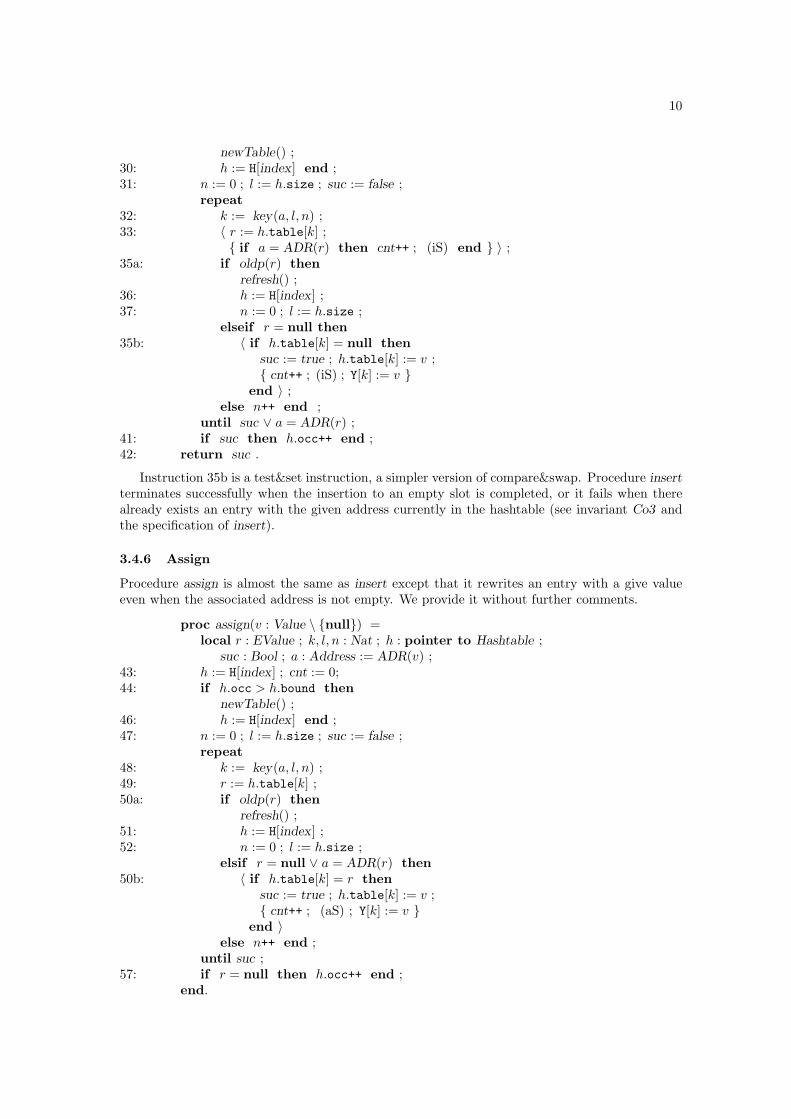
until suc ∨ a = ADR(r) ;41: if suc then h.occ++ end ;42: return suc .

Instruction 35b is a test&set instruction, a simpler version of compare&swap. Procedure insertterminates successfully when the insertion to an empty slot is completed, or it fails when therealready exists an entry with the given address currently in the hashtable (see invariant Co3 andthe specification of insert).

3.4.6 Assign

Procedure assign is almost the same as insert except that it rewrites an entry with a give valueeven when the associated address is not empty. We provide it without further comments.

proc assign(v : Value \ {null}) =local r : EValue ; k, l, n : Nat ; h : pointer to Hashtable ;

suc : Bool ; a : Address := ADR(v) ;43: h := H[index] ; cnt := 0;44: if h.occ > h.bound then

newTable() ;46: h := H[index] end ;47: n := 0 ; l := h.size ; suc := false ;

repeat48: k := key(a, l, n) ;49: r := h.table[k] ;50a: if oldp(r) then

refresh() ;51: h := H[index] ;52: n := 0 ; l := h.size ;

elsif r = null ∨ a = ADR(r) then50b: 〈 if h.table[k] = r then

suc := true ; h.table[k] := v ;{ cnt++ ; (aS) ; Y[k] := v }

end 〉else n++ end ;

until suc ;57: if r = null then h.occ++ end ;

end.

11

3.5 Memory management and concurrent migration

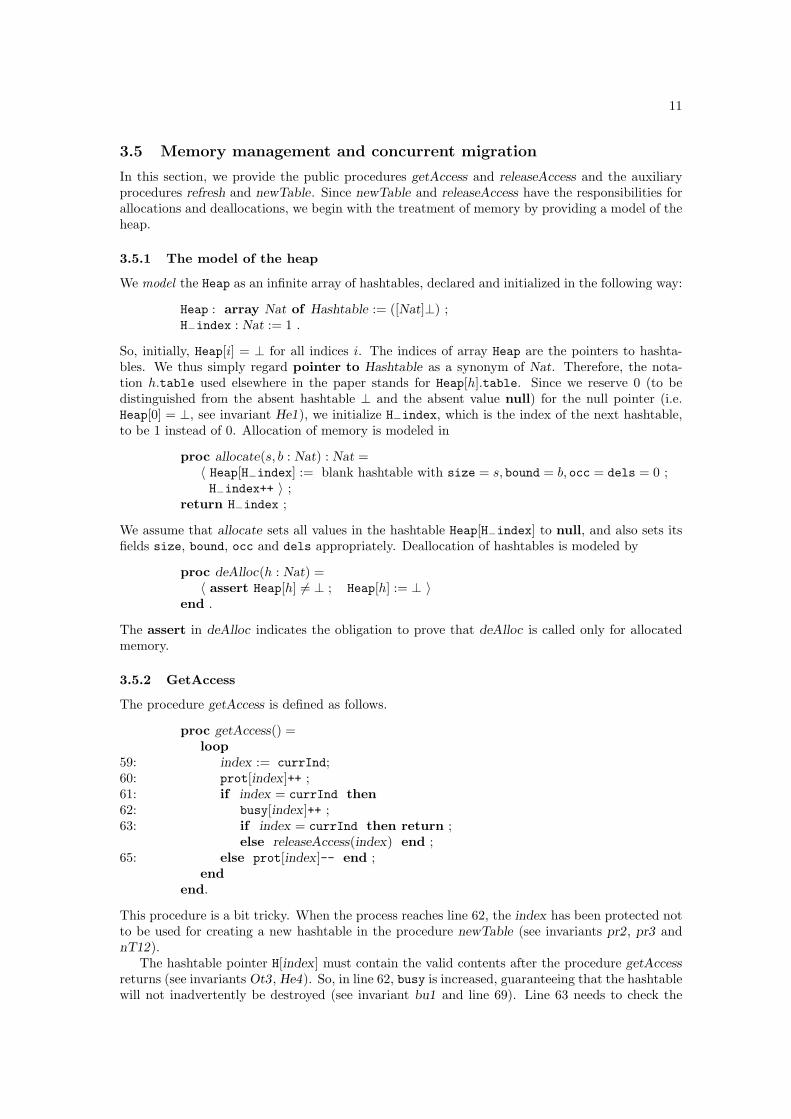
In this section, we provide the public procedures getAccess and releaseAccess and the auxiliaryprocedures refresh and newTable. Since newTable and releaseAccess have the responsibilities forallocations and deallocations, we begin with the treatment of memory by providing a model of theheap.

3.5.1 The model of the heap

We model the Heap as an infinite array of hashtables, declared and initialized in the following way:

Heap : array Nat of Hashtable := ([Nat]⊥) ;H−index : Nat := 1 .

So, initially, Heap[i] = ⊥ for all indices i. The indices of array Heap are the pointers to hashta-bles. We thus simply regard pointer to Hashtable as a synonym of Nat. Therefore, the nota-tion h.table used elsewhere in the paper stands for Heap[h].table. Since we reserve 0 (to bedistinguished from the absent hashtable ⊥ and the absent value null) for the null pointer (i.e.Heap[0] = ⊥, see invariant He1), we initialize H−index, which is the index of the next hashtable,to be 1 instead of 0. Allocation of memory is modeled in

proc allocate(s, b : Nat) : Nat =〈 Heap[H−index] := blank hashtable with size = s, bound = b, occ = dels = 0 ;H−index++ 〉 ;

return H−index ;

We assume that allocate sets all values in the hashtable Heap[H−index] to null, and also sets itsfields size, bound, occ and dels appropriately. Deallocation of hashtables is modeled by

proc deAlloc(h : Nat) =〈 assert Heap[h] 6= ⊥ ; Heap[h] := ⊥ 〉

end .

The assert in deAlloc indicates the obligation to prove that deAlloc is called only for allocatedmemory.

3.5.2 GetAccess

The procedure getAccess is defined as follows.

proc getAccess() =loop

59: index := currInd;60: prot[index]++ ;61: if index = currInd then62: busy[index]++ ;63: if index = currInd then return ;

else releaseAccess(index) end ;65: else prot[index]-- end ;

endend.

This procedure is a bit tricky. When the process reaches line 62, the index has been protected notto be used for creating a new hashtable in the procedure newTable (see invariants pr2, pr3 andnT12).

The hashtable pointer H[index] must contain the valid contents after the procedure getAccessreturns (see invariants Ot3, He4). So, in line 62, busy is increased, guaranteeing that the hashtablewill not inadvertently be destroyed (see invariant bu1 and line 69). Line 63 needs to check the

12

index again in case that instruction 62 has the precondition that the hashtable is not valid. Oncesome process gets hold of one hashtable after calling getAccess, no process can throw it away untilthe process releases it (see invariant rA7). Note that this is using releaseAccess implicitly done inrefresh.

3.5.3 ReleaseAccess

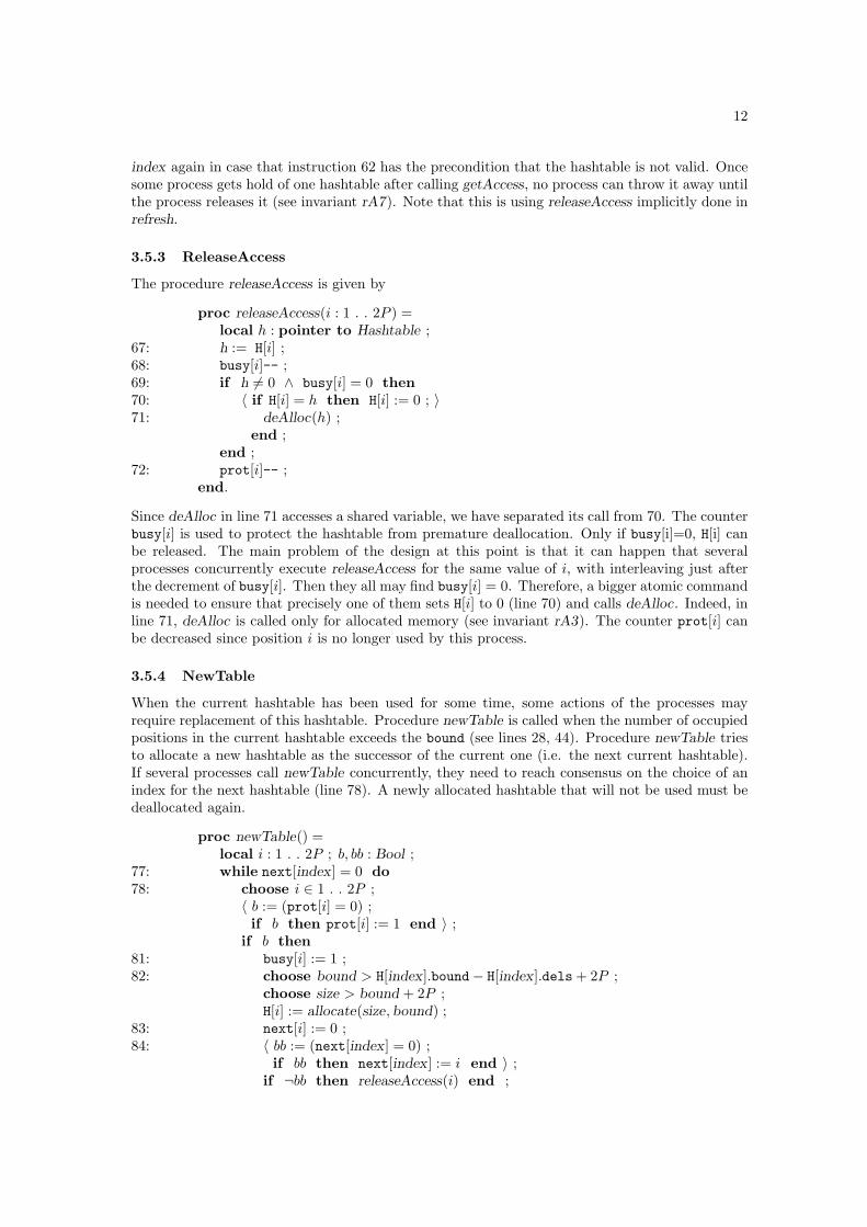
The procedure releaseAccess is given by

proc releaseAccess(i : 1 . . 2P ) =local h : pointer to Hashtable ;

67: h := H[i] ;68: busy[i]-- ;69: if h 6= 0 ∧ busy[i] = 0 then70: 〈 if H[i] = h then H[i] := 0 ; 〉71: deAlloc(h) ;

end ;end ;

72: prot[i]-- ;end.

Since deAlloc in line 71 accesses a shared variable, we have separated its call from 70. The counterbusy[i] is used to protect the hashtable from premature deallocation. Only if busy[i]=0, H[i] canbe released. The main problem of the design at this point is that it can happen that severalprocesses concurrently execute releaseAccess for the same value of i, with interleaving just afterthe decrement of busy[i]. Then they all may find busy[i] = 0. Therefore, a bigger atomic commandis needed to ensure that precisely one of them sets H[i] to 0 (line 70) and calls deAlloc. Indeed, inline 71, deAlloc is called only for allocated memory (see invariant rA3). The counter prot[i] canbe decreased since position i is no longer used by this process.

3.5.4 NewTable

When the current hashtable has been used for some time, some actions of the processes mayrequire replacement of this hashtable. Procedure newTable is called when the number of occupiedpositions in the current hashtable exceeds the bound (see lines 28, 44). Procedure newTable triesto allocate a new hashtable as the successor of the current one (i.e. the next current hashtable).If several processes call newTable concurrently, they need to reach consensus on the choice of anindex for the next hashtable (line 78). A newly allocated hashtable that will not be used must bedeallocated again.

proc newTable() =local i : 1 . . 2P ; b, bb : Bool ;

77: while next[index] = 0 do78: choose i ∈ 1 . . 2P ;

〈 b := (prot[i] = 0) ;if b then prot[i] := 1 end 〉 ;

if b then81: busy[i] := 1 ;82: choose bound > H[index].bound− H[index].dels + 2P ;

choose size > bound + 2P ;H[i] := allocate(size,bound) ;

83: next[i] := 0 ;84: 〈 bb := (next[index] = 0) ;

if bb then next[index] := i end 〉 ;if ¬bb then releaseAccess(i) end ;

13

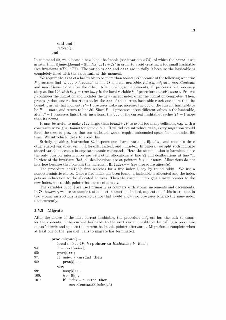
end end ;refresh() ;

end .

In command 82, we allocate a new blank hashtable (see invariant nT8), of which the bound is setgreater than H[index].bound− H[index].dels+ 2P in order to avoid creating a too small hashtable(see invariants nT6, nT7). The variables occ and dels are initially 0 because the hashtable iscompletely filled with the value null at this moment.

We require the size of a hashtable to be more than bound+2P because of the following scenario:P processes find “h.occ > h.bound” at line 28 and call newtable, refresh, migrate, moveContentsand moveElement one after the other. After moving some elements, all processes but process psleep at line 126 with bmE = true (bmE is the local variable b of procedure moveElement). Processp continues the migration and updates the new current index when the migration completes. Then,process p does several insertions to let the occ of the current hashtable reach one more than itsbound. Just at that moment, P −1 processes wake up, increase the occ of the current hashtable tobe P −1 more, and return to line 30. Since P −1 processes insert different values in the hashtable,after P − 1 processes finish their insertions, the occ of the current hashtable reaches 2P − 1 morethan its bound.

It may be useful to make size larger than bound+2P to avoid too many collisions, e.g. with aconstraint size ≥ α · bound for some α > 1. If we did not introduce dels, every migration wouldforce the sizes to grow, so that our hashtable would require unbounded space for unbounded lifetime. We introduced dels to avoid this.

Strictly speaking, instruction 82 inspects one shared variable, H[index], and modifies threeother shared variables, viz. H[i], Heap[H−index], and H−index. In general, we split such multipleshared variable accesses in separate atomic commands. Here the accumulation is harmless, sincethe only possible interferences are with other allocations at line 82 and deallocations at line 71.In view of the invariant Ha2, all deallocations are at pointers h < H−index. Allocations do notinterfere because they contain the increment H−index++ (see procedure allocate).

The procedure newTable first searches for a free index i, say by round robin. We use anondeterministic choice. Once a free index has been found, a hashtable is allocated and the indexgets an indirection to the allocated address. Then the current index gets a next pointer to thenew index, unless this pointer has been set already.

The variables prot[i] are used primarily as counters with atomic increments and decrements.In 78, however, we use an atomic test-and-set instruction. Indeed, separation of this instruction intwo atomic instructions is incorrect, since that would allow two processes to grab the same indexi concurrently.

3.5.5 Migrate

After the choice of the next current hashtable, the procedure migrate has the task to trans-fer the contents in the current hashtable to the next current hashtable by calling a proceduremoveContents and update the current hashtable pointer afterwards. Migration is complete whenat least one of the (parallel) calls to migrate has terminated.

proc migrate() =local i : 0 . . 2P ; h : pointer to Hashtable ; b : Bool ;

94: i := next[index];95: prot[i]++ ;97: if index 6= currInd then98: prot[i]-- ;

else99: busy[i]++ ;100: h := H[i] ;101: if index = currInd then

moveContents(H[index], h) ;

14

103: 〈 b := (currInd = index) ;if b then currInd := i ;

{Y := H[i].table }end 〉 ;

if b then104: busy[index]-- ;105: prot[index]-- ;

end ;end ;releaseAccess(i) ;

end end .

According to invariants mi4 and mi5, it is an invariant that i = next(index) 6= 0 holds afterinstruction 94.

Line 103 contains a compare&swap instruction to update the current hashtable pointer whensome process finds that the migration is finished while currInd is still identical to its index, whichmeans that i is still used for the next current hashtable (see invariant mi5). The increments ofprot[i] and busy[i] here are needed to protect the next hashtable. The decrements serve to avoidmemory loss.

3.5.6 Refresh

In order to avoid that a process starts migration of an old hashtable, we encapsulate migrate inrefresh in the following way.

proc refresh() =90: if index 6= currInd then

releaseAccess(index) ;getAccess() ;

else migrate() end ;end.

When index is outdated, the process needs to call releaseAccess to abandon its hashtable andgetAccess to acquire the present pointer to the current hashtable. Otherwise, the process can jointhe migration.

3.5.7 MoveContents

Procedure moveContents has to move the contents of the current table to the next current table.All processes that have access to the table, may also participate in this migration. Indeed, theycannot yet use the new table (see invariants Ne1 and Ne3). We have to take care that delayedactions on the current table and the new table are carried out or aborted correctly (see invariantsCu1 and mE10). Migration requires that every value in the current table be moved to a uniqueposition in the new table (see invariant Ne19).

Procedure moveContents uses a private variable toBeMoved that ranges over sets of locations.The procedure is given by

proc moveContents(from, to : pointer to Hashtable) =local i : Nat ; b : Bool ; v : EValue} ; toBeMoved : set of Nat ;toBeMoved := {0, . . . , from.size− 1} ;

110: while currInd = index ∧ toBeMoved 6= ∅ do111: choose i ∈ toBeMoved ;

v := from.table[i] ;if from.table[i] = done then

118: toBeMoved := toBeMoved − {i} ;else

15

114: 〈 b := (v = from.table[i]) ;if b then from.table[i] := old(val(v)) end 〉 ;

if b then116: if val(v) 6= null then moveElement(val(v), to) end ;117: from.table[i] := done ;118: toBeMoved := toBeMoved − {i} ;

end end end ;end .

Note that the value is tagged as outdated before being duplicated (see invariant mC11). Aftertagging, the value cannot be deleted or assigned until the migration has been completed. Taggingmust be done atomically, since otherwise an interleaving deletion may be lost. When indeed thevalue has been copied to the new hashtable, in line 117 that value becomes done in the hashtable.This has the effect that other processes need not wait for this process to complete proceduremoveElement, but can help with the migration of this value if needed.

Since the address is lost after being rewritten to done, we had to introduce the shared auxiliaryhashtable Y to remember its value for the proof of correctness. This could have been avoided byintroducing a second tagging bit, say for “very old”.

The processes involved in the same migration should not use the same strategy for choosing iin line 111, since it is advantageous that moveElement is called often with different values. Theymay exchange information: any of them may replace its set toBeMoved by the intersection of thatset with the set toBeMoved of another one. We do not give a preferred strategy here, one canrefer to algorithms for the write-all problem [4, 13].

3.5.8 MoveElement

The procedure moveElement moves a value to the new hashtable. Note that the value is taggedas outdated in moveContents before moveElement is called.

proc moveElement(v : Value \ {null}, to : pointer to Hashtable) =local a : Address ; k,m, n : Nat ; w : EValue ; b : Bool ;

120: n := 0 ; b := false ; a := ADR(v) ; m := to.size ;repeat

121: k := key(a,m, n) ; w := to.table[k] ;if w = null then

123: 〈 b := (to.table[k] = null);if b then to.table[k] := v end 〉 ;

else n++ end ;125: until b ∨ a = ADR(w) ∨ currInd 6= index ;126: if b then to.occ++ end

end .

The value is only allowed to be inserted once in the new hashtable (see invariant Ne19),otherwise it will violate the main property of open addressing. In total, four situations can occurin the procedure moveElement:

• the current location k contains a value with an other address, the process will increase nand inspect the next location.

• the current location k contains a value with the same address, which means the value hasbeen copied to the new hashtable already. The process therefore terminates.

• the current location k is an empty slot. The process inserts v and returns. If insertion fails,as an other process did fill the empty slot, the search is continued.

• when index happens to differ from currInd, the whole migration has been completed.

16

While the current hashtable pointer is not updated yet, there exists at least one null entry inthe new hashtable (see invariants Ne8, Ne22 and Ne23), hence the local variable n in the proceduremoveElement never goes beyond the size of the hashtable (see invariants mE3 and mE8), and thetermination is thus guaranteed.

4 Correctness (Safety)

In this section, we describe the proof of safety of the algorithm. The main aspects of safety arefunctional correctness, atomicity, and absence of memory loss. These aspects are formalized ineight invariants described in section 4.1. To prove these invariants, we need many other invariants.These are listed in Appendix A. In section 4.2, we sketch the verification of some of the invariantsby informal means. In section 4.3, we describe how the theorem prover PVS is used in theverification. As exemplified in 4.2, Appendix B gives the dependencies between the invariants.

Notational Conventions. Recall that there are at most P processes with process identifiersranging from 1 up to P . We use p, q, r to range over process identifiers, with a preference forp. Since the same program is executed by all processes, every private variable name of a process6= p is extended with the suffix “.” + “process identifier”. We do not do this for process p. So,e.g., the value of a private variable x of process q is denoted by x.q, but the value of x of processp is just denoted by x. In particular, pc.q is the program location of process q. It ranges over allinteger labels used in the implementation.

When local variables in different procedures have the same names, we add an abbreviation ofthe procedure name as a subscript to the name. We use the following abbreviations: fi for find, delfor delete, ins for insert, ass for assign, gA for getAccess, rA for releaseAccess, nT for newTable,mig for migrate, ref for refresh, mC for moveContents, mE for moveElement.

In the implementation, there are several places where the same procedure is called, saygetAccess, releaseAccess, etc. We introduce auxiliary private variables return, local to such aprocedure, to hold the return location. We add a procedure subscript to distinguish these vari-ables according to the above convention.

If V is a set, ]V denotes the number of elements of V . If b is a boolean, then ]b = 0 whenb is false, and ]b = 1 when b is true. Unless explicitly defined otherwise, we always (implicitly)universally quantify over addresses a, values v, non-negative integer numbers k, m, and n, naturalnumber l, processes p, q and r. Indices i and j range over [1, 2P ]. We abbreviate H(currInd).sizeas curSize.

In order to avoid using too many parentheses, we use the usual binding order for the operators.We give “∧” higher priority than “∨”. We use parentheses whenever necessary.

4.1 Main properties

We have proved the following three safety properties of the algorithm. Firstly, the access proce-dures find, delete, insert, assign, are functionally correct. Secondly they are executed atomically.The third safety property is absence of memory loss.

Functional correctness of find, delete, insert is the condition that the result of the implementa-tion is the same as the result of the specification (fS), (dS), (iS). This is expressed by the requiredinvariants:

Co1: pc = 14 ⇒ val(rfi) = rSfi

Co2: pc ∈ {25, 26} ⇒ sucdel = sucSdel

Co3: pc ∈ {41, 42} ⇒ sucins = sucSins

Note that functional correctness of assign holds trivially since it does not return a result.According to the definition of atomicity in chapter 13 of [16], atomicity means that each

execution of one of the access procedures contains precisely one execution of the correspondingspecifying action (fS), (dS), (iS), (aS). We introduced the private auxiliary variables cnt to count

17

the number of times the specifying action is executed. Therefore, atomicity is expressed by theinvariants:

Cn1: pc = 14 ⇒ cntfi = 1Cn2: pc ∈ {25, 26} ⇒ cntdel = 1Cn3: pc ∈ {41, 42} ⇒ cntins = 1Cn4: pc = 57 ⇒ cntass = 1

We interpret absence of memory loss to mean that the number of valid hashtables is bounded.More precisely, we prove that this number is bounded by 2P . This is formalized in the invariant:

No1: ]{k | k < H−index ∧ Heap(k) 6= ⊥} ≤ 2P

4.2 Intuitive proof

The eight correctness properties (invariants) mentioned above have been completely proved withthe interactive proof checker of PVS. The use of PVS did not only take care of the delicatebookkeeping involved in the proof, it could also deal with many trivial cases automatically. Atseveral occasions where PVS refused to let a proof be finished, we actually found a mistake andhad to correct previous versions of this algorithm.

In order to give some feeling for the proof, we describe some proofs. For the complete mechan-ical proof, we refer the reader to [12]. Note that, for simplicity, we assume that all non-specificprivate variables in the proposed assertions belong to the general process p, and general process qis an active process that tries to threaten some assertion (p may equal q).

Proof of invariant Co1 (as claimed in 4.1). According to Appendix B, the stability of Co1 followsfrom the invariants Ot3, fi1, fi10, which are given in Appendix A. Indeed, Ot3 implies that noprocedure returns to location 14. Therefore all return statements falsify the antecedent of Co1 andthus preserve Co1. Since rfi and rSfi are private variables to process p, Co1 can only be violatedby process p itself (establishing pc at 14) when p executes 13 with rfi = null ∨ afi = ADR(rfi).This condition is abbreviated as Find(rfi , afi). Invariant fi10 then implies that action 13 has theprecondition val(rfi) = rSfi , so then it does not violate Co1. In PVS, we used a slightly differentdefinition of Find, and we applied invariant fi1 to exclude that rfi is done or del, though invariantfi1 is superfluous in this intuitive proof. 2

Proof of invariant Ot3. Since the procedures getAccess, releaseAccess, refresh, newTable arecalled only at specific locations in the algorithm, it is easy to list the potential return addresses.Since the variables return are private to process p, they are not modified by other processes. Sta-bility of Ot3 follows from this. As we saw in the previous proof, Ot3 is used to guarantee that nounexpected jumps occur. 2

Proof of invariant fi10. According to Appendix B, we only need to use fi9 and Ot3. Let us usethe abbreviation k = key(afi , lfi , nfi). Since rfi and rSfi are both private variables, they can onlybe modified by process p when p is executing statement 7. We split this situation into two cases

1. with precondition Find(hfi .table[k], afi)After execution of statement 7, rfi becomes hfi .table[k], and rSfi becomes X(afi). By fi9,we get val(rfi) = rSfi . Therefore the validity of fi10 is preserved.

2. otherwise.After execution of statement 7, rfi becomes hfi .table[k], which then falsifies the antecedentof fi10. 2

Proof of invariant fi9. According to Appendix B, we proved that fi9 follows from Ax2, fi1, fi3,fi4, fi5, fi8, Ha4, He4, Cu1, Cu9, Cu10, and Cu11. We abbreviate key(afi , lfi , nfi) as k. We

18

deduce hfi = H(index) from fi4, H(index) is not ⊥ from He4, and k is below H(index).size fromAx2, fi4 and fi3. We split the proof into two cases:

1. index 6= currInd: By Ha4, it follows that H(index) 6= H(currInd). Hence from Cu1, weobtain hfi .table[k] = done, which falsifies the antecedent of fi9.

2. index = currInd: By premise Find(hfi .table[k], afi), we know that hfi .table[k] 6= donebecause of fi1. By Cu9 and Cu10, we obtain val(hfi .table[k]) = val(Y[k]). Hence it followsthat Find(Y[k], afi). Using fi8, we obtain

∀m < nfi : ¬Find(Y[key(afi , curSize,m)], afi)

We get nfi is below curSize because of fi5. By Cu11, we conclude

X(afi) = val(hfi .table[k])2

4.3 The model in PVS

Our proof architecture (for one property) can be described as a dynamically growing tree in whicheach node is associated with an assertion. We start from a tree containing only one node, theproof goal, which characterizes some property of the system. We expand the tree by adding somenew children via proper analysis of an unproved node (top-down approach, which requires a goodunderstanding of the system). The validity of that unproved node is then reduced to the validityof its children and the validity of some less or equally deep nodes.

Normally, simple properties of the system are proved with appropriate precedence, and thenused to help establish more complex ones. It is not a bad thing that some property that was takenfor granted turns out to be not valid. Indeed, it may uncover a defect of the algorithm, but in anycase it leads to new insights in it.

We model the algorithm as a transition system [17], which is described in the language of PVSin the following way. As usual in PVS, states are represented by a record with a number of fields:

State : TYPE = [#% global variables

...busy : [ range(2*P) → nat ],prot : [ range(2*P) → nat ],...

% private variables:index : [ range(P) → range(2*P) ],...pc : [ range(P) → nat ], % private program counters...

% local variables of procedures, also private to each process:% find

a−find : [ range(P) → Address ],r−find : [ range(P) → EValue ],...

% getAccessreturn−getAccess : [ range(P) → nat ],...

#]

where range(P) stands for the range of integers from 1 to P.Note that private variables are given with as argument a process identifier. Local variables are

distinguished by adding their procedure’s names as suffixes.

19

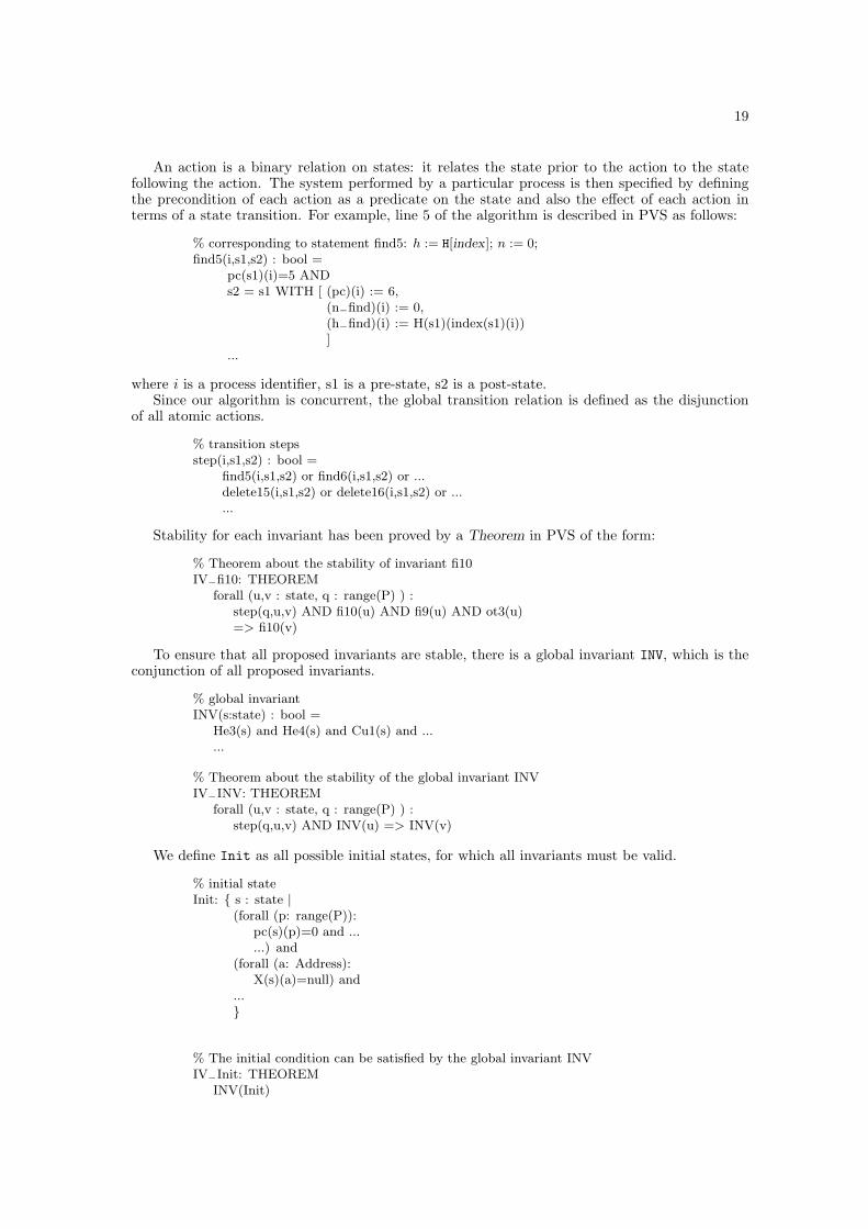
An action is a binary relation on states: it relates the state prior to the action to the statefollowing the action. The system performed by a particular process is then specified by definingthe precondition of each action as a predicate on the state and also the effect of each action interms of a state transition. For example, line 5 of the algorithm is described in PVS as follows:

% corresponding to statement find5: h := H[index]; n := 0;find5(i,s1,s2) : bool =

pc(s1)(i)=5 ANDs2 = s1 WITH [ (pc)(i) := 6,

(n−find)(i) := 0,(h−find)(i) := H(s1)(index(s1)(i))]

...

where i is a process identifier, s1 is a pre-state, s2 is a post-state.Since our algorithm is concurrent, the global transition relation is defined as the disjunction

of all atomic actions.

% transition stepsstep(i,s1,s2) : bool =

find5(i,s1,s2) or find6(i,s1,s2) or ...delete15(i,s1,s2) or delete16(i,s1,s2) or ......

Stability for each invariant has been proved by a Theorem in PVS of the form:

% Theorem about the stability of invariant fi10IV−fi10: THEOREM

forall (u,v : state, q : range(P) ) :step(q,u,v) AND fi10(u) AND fi9(u) AND ot3(u)=> fi10(v)

To ensure that all proposed invariants are stable, there is a global invariant INV, which is theconjunction of all proposed invariants.

% global invariantINV(s:state) : bool =

He3(s) and He4(s) and Cu1(s) and ......

% Theorem about the stability of the global invariant INVIV−INV: THEOREM

forall (u,v : state, q : range(P) ) :step(q,u,v) AND INV(u) => INV(v)

We define Init as all possible initial states, for which all invariants must be valid.

% initial stateInit: { s : state |

(forall (p: range(P)):pc(s)(p)=0 and ......) and

(forall (a: Address):X(s)(a)=null) and

...}

% The initial condition can be satisfied by the global invariant INVIV−Init: THEOREM

INV(Init)

20

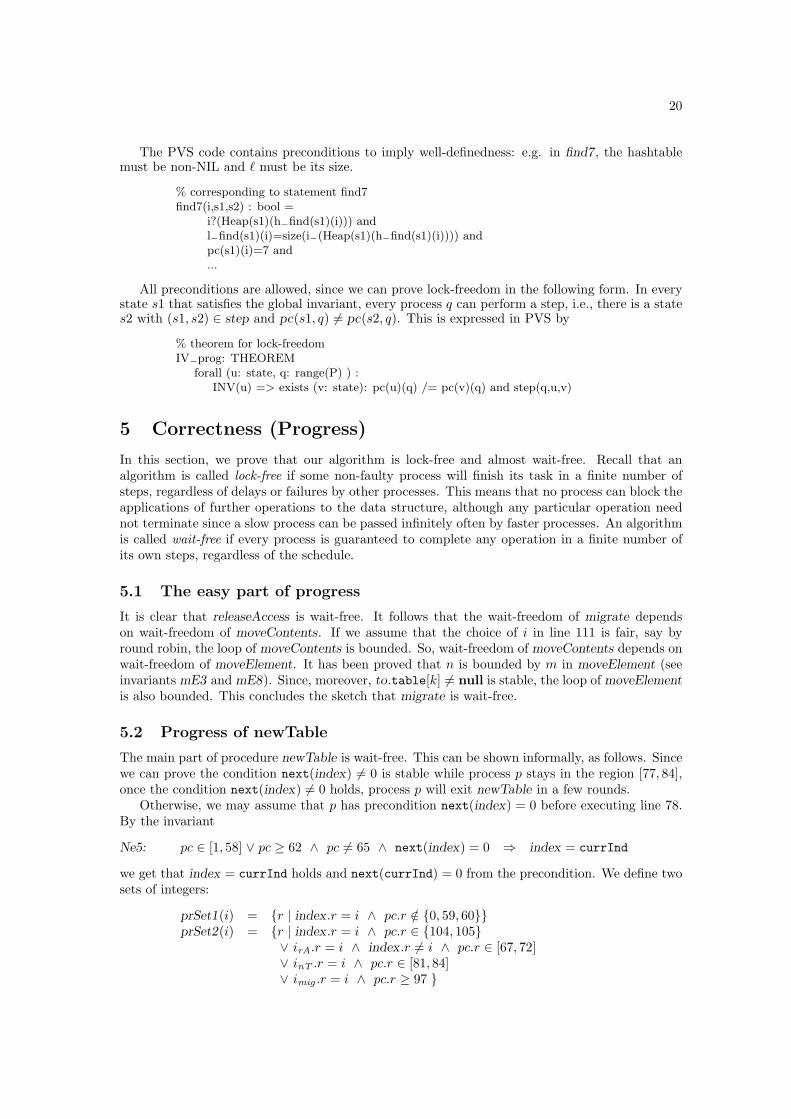
The PVS code contains preconditions to imply well-definedness: e.g. in find7, the hashtablemust be non-NIL and ` must be its size.

% corresponding to statement find7find7(i,s1,s2) : bool =

i?(Heap(s1)(h−find(s1)(i))) andl−find(s1)(i)=size(i−(Heap(s1)(h−find(s1)(i)))) andpc(s1)(i)=7 and...

All preconditions are allowed, since we can prove lock-freedom in the following form. In everystate s1 that satisfies the global invariant, every process q can perform a step, i.e., there is a states2 with (s1, s2) ∈ step and pc(s1, q) 6= pc(s2, q). This is expressed in PVS by

% theorem for lock-freedomIV−prog: THEOREM

forall (u: state, q: range(P) ) :INV(u) => exists (v: state): pc(u)(q) /= pc(v)(q) and step(q,u,v)

5 Correctness (Progress)

In this section, we prove that our algorithm is lock-free and almost wait-free. Recall that analgorithm is called lock-free if some non-faulty process will finish its task in a finite number ofsteps, regardless of delays or failures by other processes. This means that no process can block theapplications of further operations to the data structure, although any particular operation neednot terminate since a slow process can be passed infinitely often by faster processes. An algorithmis called wait-free if every process is guaranteed to complete any operation in a finite number ofits own steps, regardless of the schedule.

5.1 The easy part of progress

It is clear that releaseAccess is wait-free. It follows that the wait-freedom of migrate dependson wait-freedom of moveContents. If we assume that the choice of i in line 111 is fair, say byround robin, the loop of moveContents is bounded. So, wait-freedom of moveContents depends onwait-freedom of moveElement. It has been proved that n is bounded by m in moveElement (seeinvariants mE3 and mE8). Since, moreover, to.table[k] 6= null is stable, the loop of moveElementis also bounded. This concludes the sketch that migrate is wait-free.

5.2 Progress of newTable

The main part of procedure newTable is wait-free. This can be shown informally, as follows. Sincewe can prove the condition next(index) 6= 0 is stable while process p stays in the region [77, 84],once the condition next(index) 6= 0 holds, process p will exit newTable in a few rounds.

Otherwise, we may assume that p has precondition next(index) = 0 before executing line 78.By the invariant

Ne5: pc ∈ [1, 58] ∨ pc ≥ 62 ∧ pc 6= 65 ∧ next(index) = 0 ⇒ index = currInd

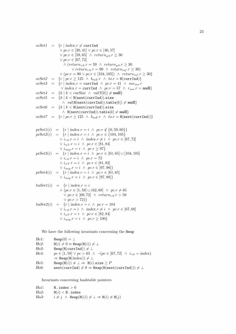
we get that index = currInd holds and next(currInd) = 0 from the precondition. We define twosets of integers:

prSet1(i) = {r | index.r = i ∧ pc.r /∈ {0, 59, 60}}prSet2(i) = {r | index.r = i ∧ pc.r ∈ {104, 105}

∨ irA.r = i ∧ index.r 6= i ∧ pc.r ∈ [67, 72]∨ inT .r = i ∧ pc.r ∈ [81, 84]∨ imig .r = i ∧ pc.r ≥ 97 }

21

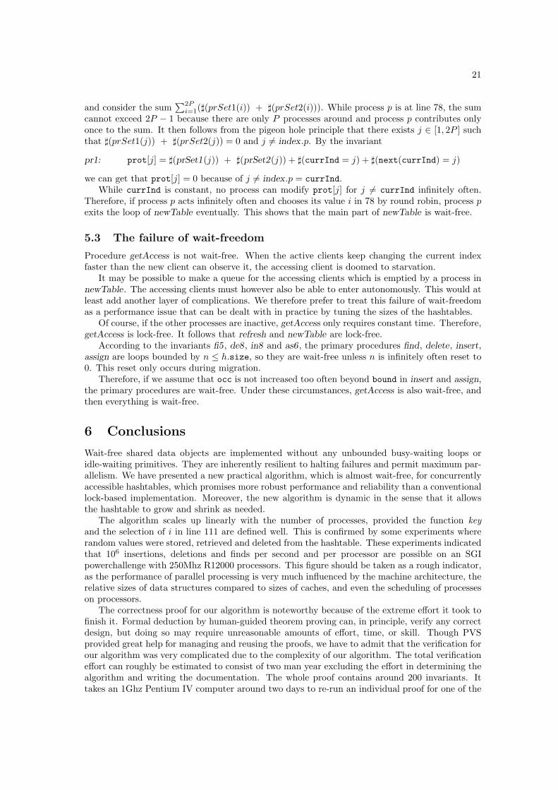
and consider the sum∑2P

i=1(](prSet1(i)) + ](prSet2(i))). While process p is at line 78, the sumcannot exceed 2P − 1 because there are only P processes around and process p contributes onlyonce to the sum. It then follows from the pigeon hole principle that there exists j ∈ [1, 2P ] suchthat ](prSet1(j)) + ](prSet2(j)) = 0 and j 6= index.p. By the invariant

pr1: prot[j] = ](prSet1(j)) + ](prSet2(j)) + ](currInd = j) + ](next(currInd) = j)

we can get that prot[j] = 0 because of j 6= index.p = currInd.While currInd is constant, no process can modify prot[j] for j 6= currInd infinitely often.

Therefore, if process p acts infinitely often and chooses its value i in 78 by round robin, process pexits the loop of newTable eventually. This shows that the main part of newTable is wait-free.

5.3 The failure of wait-freedom

Procedure getAccess is not wait-free. When the active clients keep changing the current indexfaster than the new client can observe it, the accessing client is doomed to starvation.

It may be possible to make a queue for the accessing clients which is emptied by a process innewTable. The accessing clients must however also be able to enter autonomously. This would atleast add another layer of complications. We therefore prefer to treat this failure of wait-freedomas a performance issue that can be dealt with in practice by tuning the sizes of the hashtables.

Of course, if the other processes are inactive, getAccess only requires constant time. Therefore,getAccess is lock-free. It follows that refresh and newTable are lock-free.

According to the invariants fi5, de8, in8 and as6, the primary procedures find, delete, insert,assign are loops bounded by n ≤ h.size, so they are wait-free unless n is infinitely often reset to0. This reset only occurs during migration.

Therefore, if we assume that occ is not increased too often beyond bound in insert and assign,the primary procedures are wait-free. Under these circumstances, getAccess is also wait-free, andthen everything is wait-free.

6 Conclusions

Wait-free shared data objects are implemented without any unbounded busy-waiting loops oridle-waiting primitives. They are inherently resilient to halting failures and permit maximum par-allelism. We have presented a new practical algorithm, which is almost wait-free, for concurrentlyaccessible hashtables, which promises more robust performance and reliability than a conventionallock-based implementation. Moreover, the new algorithm is dynamic in the sense that it allowsthe hashtable to grow and shrink as needed.

The algorithm scales up linearly with the number of processes, provided the function keyand the selection of i in line 111 are defined well. This is confirmed by some experiments whererandom values were stored, retrieved and deleted from the hashtable. These experiments indicatedthat 106 insertions, deletions and finds per second and per processor are possible on an SGIpowerchallenge with 250Mhz R12000 processors. This figure should be taken as a rough indicator,as the performance of parallel processing is very much influenced by the machine architecture, therelative sizes of data structures compared to sizes of caches, and even the scheduling of processeson processors.

The correctness proof for our algorithm is noteworthy because of the extreme effort it took tofinish it. Formal deduction by human-guided theorem proving can, in principle, verify any correctdesign, but doing so may require unreasonable amounts of effort, time, or skill. Though PVSprovided great help for managing and reusing the proofs, we have to admit that the verification forour algorithm was very complicated due to the complexity of our algorithm. The total verificationeffort can roughly be estimated to consist of two man year excluding the effort in determining thealgorithm and writing the documentation. The whole proof contains around 200 invariants. Ittakes an 1Ghz Pentium IV computer around two days to re-run an individual proof for one of the

22

biggest invariants. Without suitable tool support like PVS, we even doubt if it would be possibleto complete a reliable proof of such size and complexity.

Probably, it is possible to simplify the proof and reduce the number of invariants a little bit,but we did not work on this. The complete version of the PVS specifications and the whole proofscripts can be found at [12]. Note that we simplified some definitions in the paper for the sake ofpresentation.

A Invariants

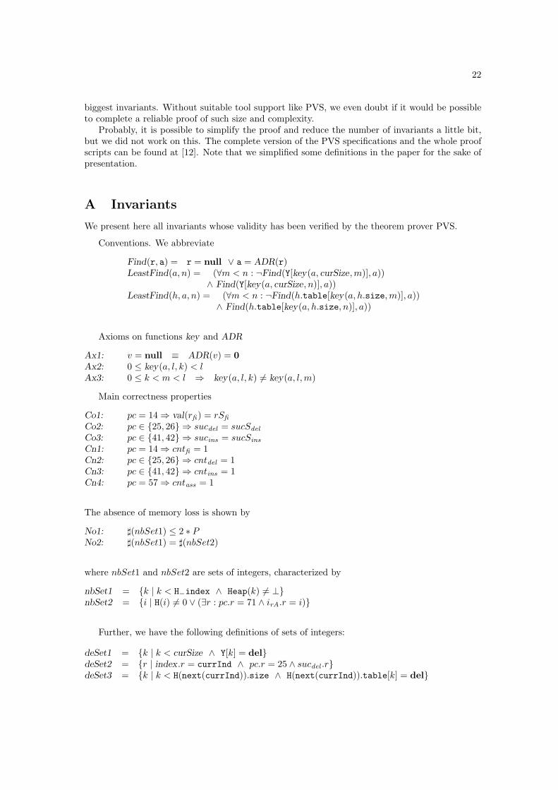
We present here all invariants whose validity has been verified by the theorem prover PVS.

Conventions. We abbreviate

Find(r, a) = r = null ∨ a = ADR(r)LeastFind(a, n) = (∀m < n : ¬Find(Y[key(a, curSize,m)], a))

∧ Find(Y[key(a, curSize, n)], a))LeastFind(h, a, n) = (∀m < n : ¬Find(h.table[key(a, h.size,m)], a))

∧ Find(h.table[key(a, h.size, n)], a))

Axioms on functions key and ADR

Ax1: v = null ≡ ADR(v) = 0Ax2: 0 ≤ key(a, l, k) < lAx3: 0 ≤ k < m < l ⇒ key(a, l, k) 6= key(a, l,m)

Main correctness properties

Co1: pc = 14 ⇒ val(rfi) = rSfi

Co2: pc ∈ {25, 26} ⇒ sucdel = sucSdel

Co3: pc ∈ {41, 42} ⇒ sucins = sucSins

Cn1: pc = 14 ⇒ cntfi = 1Cn2: pc ∈ {25, 26} ⇒ cntdel = 1Cn3: pc ∈ {41, 42} ⇒ cntins = 1Cn4: pc = 57 ⇒ cntass = 1

The absence of memory loss is shown by

No1: ](nbSet1) ≤ 2 ∗ PNo2: ](nbSet1) = ](nbSet2)

where nbSet1 and nbSet2 are sets of integers, characterized by

nbSet1 = {k | k < H−index ∧ Heap(k) 6= ⊥}nbSet2 = {i | H(i) 6= 0 ∨ (∃r : pc.r = 71 ∧ irA.r = i)}

Further, we have the following definitions of sets of integers:

deSet1 = {k | k < curSize ∧ Y[k] = del}deSet2 = {r | index.r = currInd ∧ pc.r = 25 ∧ sucdel .r}deSet3 = {k | k < H(next(currInd)).size ∧ H(next(currInd)).table[k] = del}

23

ocSet1 = {r | index.r 6= currInd∨ pc.r ∈ [30, 41] ∨ pc.r ∈ [46, 57]∨ pc.r ∈ [59, 65] ∧ returngA.r ≥ 30∨ pc.r ∈ [67, 72]∧ (returnrA.r = 59 ∧ returngA.r ≥ 30

∨ returnrA.r = 90 ∧ returnref .r ≥ 30)∨ (pc.r = 90 ∨ pc.r ∈ [104, 105]) ∧ returnref .r ≥ 30}

ocSet2 = {r | pc.r ≥ 125 ∧ bmE .r ∧ to.r = H(currInd)}ocSet3 = {r | index.r = currInd ∧ pc.r = 41 ∧ sucins .r

∨ index.r = currInd ∧ pc.r = 57 ∧ rass .r = null}ocSet4 = {k | k < curSize ∧ val(Y[k]) 6= null}ocSet5 = {k | k < H(next(currInd)).size

∧ val(H(next(currInd)).table[k]) 6= null}ocSet6 = {k | k < H(next(currInd)).size

∧ H(next(currInd)).table[k] 6= null}ocSet7 = {r | pc.r ≥ 125 ∧ bmE .r ∧ to.r = H(next(currInd))}

prSet1(i) = {r | index.r = i ∧ pc.r /∈ {0, 59, 60}}prSet2(i) = {r | index.r = i ∧ pc.r ∈ {104, 105}

∨ irA.r = i ∧ index.r 6= i ∧ pc.r ∈ [67, 72]∨ inT .r = i ∧ pc.r ∈ [81, 84]∨ imig .r = i ∧ pc.r ≥ 97}

prSet3(i) = {r | index.r = i ∧ pc.r ∈ [61, 65] ∪ [104, 105]∨ irA.r = i ∧ pc.r = 72∨ inT .r = i ∧ pc.r ∈ [81, 82]∨ imig .r = i ∧ pc.r ∈ [97, 98]}

prSet4(i) = {r | index.r = i ∧ pc.r ∈ [61, 65]∨ imig .r = i ∧ pc.r ∈ [97, 98]}

buSet1(i) = {r | index.r = i∧ (pc.r ∈ [1, 58] ∪ (62, 68] ∧ pc.r 6= 65∨ pc.r ∈ [69, 72] ∧ returnrA.r > 59∨ pc.r > 72)}

buSet2(i) = {r | index.r = i ∧ pc.r = 104∨ irA.r = i ∧ index.r 6= i ∧ pc.r ∈ [67, 68]∨ inT .r = i ∧ pc.r ∈ [82, 84]∨ imig .r = i ∧ pc.r ≥ 100}

We have the following invariants concerning the Heap

He1: Heap(0) = ⊥He2: H(i) 6= 0 ≡ Heap(H(i)) 6= ⊥He3: Heap(H(currInd)) 6= ⊥He4: pc ∈ [1, 58] ∨ pc > 65 ∧ ¬(pc ∈ [67, 72] ∧ irA = index)

⇒ Heap(H(index)) 6= ⊥He5: Heap(H(i)) 6= ⊥ ⇒ H(i).size ≥ PHe6: next(currInd) 6= 0 ⇒ Heap(H(next(currInd))) 6= ⊥

Invariants concerning hashtable pointers

Ha1: H−index > 0Ha2: H(i) < H−indexHa3: i 6= j ∧ Heap(H(i)) 6= ⊥ ⇒ H(i) 6= H(j)

24

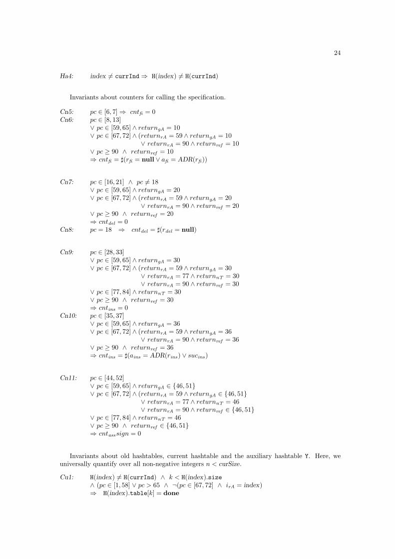
Ha4: index 6= currInd⇒ H(index) 6= H(currInd)

Invariants about counters for calling the specification.

Cn5: pc ∈ [6, 7] ⇒ cntfi = 0Cn6: pc ∈ [8, 13]

∨ pc ∈ [59, 65] ∧ returngA = 10∨ pc ∈ [67, 72] ∧ (returnrA = 59 ∧ returngA = 10

∨ returnrA = 90 ∧ returnref = 10∨ pc ≥ 90 ∧ returnref = 10⇒ cntfi = ](rfi = null ∨ afi = ADR(rfi))

Cn7: pc ∈ [16, 21] ∧ pc 6= 18∨ pc ∈ [59, 65] ∧ returngA = 20∨ pc ∈ [67, 72] ∧ (returnrA = 59 ∧ returngA = 20

∨ returnrA = 90 ∧ returnref = 20∨ pc ≥ 90 ∧ returnref = 20⇒ cntdel = 0

Cn8: pc = 18 ⇒ cntdel = ](rdel = null)

Cn9: pc ∈ [28, 33]∨ pc ∈ [59, 65] ∧ returngA = 30∨ pc ∈ [67, 72] ∧ (returnrA = 59 ∧ returngA = 30

∨ returnrA = 77 ∧ returnnT = 30∨ returnrA = 90 ∧ returnref = 30

∨ pc ∈ [77, 84] ∧ returnnT = 30∨ pc ≥ 90 ∧ returnref = 30⇒ cntins = 0

Cn10: pc ∈ [35, 37]∨ pc ∈ [59, 65] ∧ returngA = 36∨ pc ∈ [67, 72] ∧ (returnrA = 59 ∧ returngA = 36

∨ returnrA = 90 ∧ returnref = 36∨ pc ≥ 90 ∧ returnref = 36⇒ cntins = ](ains = ADR(rins) ∨ sucins)

Cn11: pc ∈ [44, 52]∨ pc ∈ [59, 65] ∧ returngA ∈ {46, 51}∨ pc ∈ [67, 72] ∧ (returnrA = 59 ∧ returngA ∈ {46, 51}

∨ returnrA = 77 ∧ returnnT = 46∨ returnrA = 90 ∧ returnref ∈ {46, 51}

∨ pc ∈ [77, 84] ∧ returnnT = 46∨ pc ≥ 90 ∧ returnref ∈ {46, 51}⇒ cntasssign = 0

Invariants about old hashtables, current hashtable and the auxiliary hashtable Y. Here, weuniversally quantify over all non-negative integers n < curSize.

Cu1: H(index) 6= H(currInd) ∧ k < H(index).size∧ (pc ∈ [1, 58] ∨ pc > 65 ∧ ¬(pc ∈ [67, 72] ∧ irA = index)⇒ H(index).table[k] = done

25

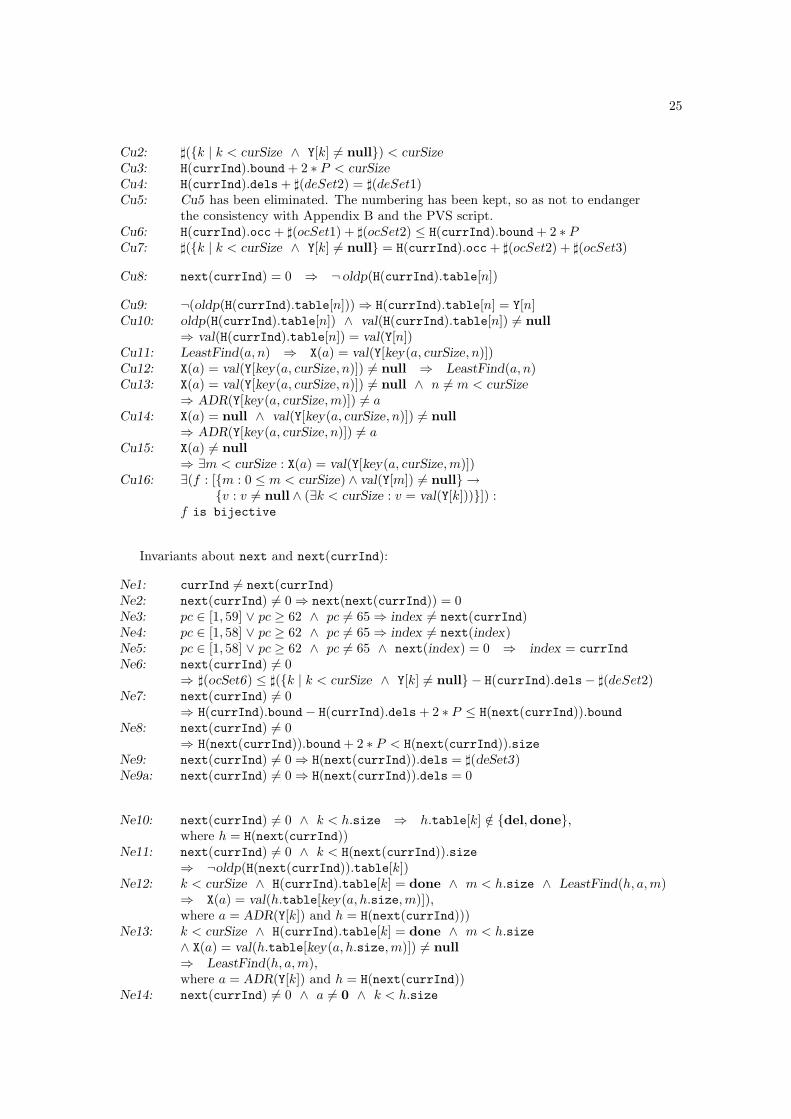
Cu2: ]({k | k < curSize ∧ Y[k] 6= null}) < curSizeCu3: H(currInd).bound + 2 ∗ P < curSizeCu4: H(currInd).dels + ](deSet2) = ](deSet1)Cu5: Cu5 has been eliminated. The numbering has been kept, so as not to endanger

the consistency with Appendix B and the PVS script.Cu6: H(currInd).occ + ](ocSet1) + ](ocSet2) ≤ H(currInd).bound + 2 ∗ PCu7: ]({k | k < curSize ∧ Y[k] 6= null} = H(currInd).occ + ](ocSet2) + ](ocSet3)

Cu8: next(currInd) = 0 ⇒ ¬ oldp(H(currInd).table[n])

Cu9: ¬(oldp(H(currInd).table[n])) ⇒ H(currInd).table[n] = Y[n]Cu10: oldp(H(currInd).table[n]) ∧ val(H(currInd).table[n]) 6= null

⇒ val(H(currInd).table[n]) = val(Y[n])Cu11: LeastFind(a, n) ⇒ X(a) = val(Y[key(a, curSize, n)])Cu12: X(a) = val(Y[key(a, curSize, n)]) 6= null ⇒ LeastFind(a, n)Cu13: X(a) = val(Y[key(a, curSize, n)]) 6= null ∧ n 6= m < curSize

⇒ ADR(Y[key(a, curSize,m)]) 6= aCu14: X(a) = null ∧ val(Y[key(a, curSize, n)]) 6= null

⇒ ADR(Y[key(a, curSize, n)]) 6= aCu15: X(a) 6= null

⇒ ∃m < curSize : X(a) = val(Y[key(a, curSize,m)])Cu16: ∃(f : [{m : 0 ≤ m < curSize) ∧ val(Y[m]) 6= null} →

{v : v 6= null ∧ (∃k < curSize : v = val(Y[k]))}]) :f is bijective

Invariants about next and next(currInd):

Ne1: currInd 6= next(currInd)Ne2: next(currInd) 6= 0 ⇒ next(next(currInd)) = 0Ne3: pc ∈ [1, 59] ∨ pc ≥ 62 ∧ pc 6= 65 ⇒ index 6= next(currInd)Ne4: pc ∈ [1, 58] ∨ pc ≥ 62 ∧ pc 6= 65 ⇒ index 6= next(index)Ne5: pc ∈ [1, 58] ∨ pc ≥ 62 ∧ pc 6= 65 ∧ next(index) = 0 ⇒ index = currIndNe6: next(currInd) 6= 0

⇒ ](ocSet6) ≤ ]({k | k < curSize ∧ Y[k] 6= null} − H(currInd).dels− ](deSet2)Ne7: next(currInd) 6= 0

⇒ H(currInd).bound− H(currInd).dels + 2 ∗ P ≤ H(next(currInd)).boundNe8: next(currInd) 6= 0

⇒ H(next(currInd)).bound + 2 ∗ P < H(next(currInd)).sizeNe9: next(currInd) 6= 0 ⇒ H(next(currInd)).dels = ](deSet3)Ne9a: next(currInd) 6= 0 ⇒ H(next(currInd)).dels = 0

Ne10: next(currInd) 6= 0 ∧ k < h.size ⇒ h.table[k] /∈ {del,done},where h = H(next(currInd))

Ne11: next(currInd) 6= 0 ∧ k < H(next(currInd)).size⇒ ¬oldp(H(next(currInd)).table[k])

Ne12: k < curSize ∧ H(currInd).table[k] = done ∧ m < h.size ∧ LeastFind(h, a,m)⇒ X(a) = val(h.table[key(a, h.size,m)]),where a = ADR(Y[k]) and h = H(next(currInd)))

Ne13: k < curSize ∧ H(currInd).table[k] = done ∧ m < h.size∧ X(a) = val(h.table[key(a, h.size,m)]) 6= null⇒ LeastFind(h, a,m),where a = ADR(Y[k]) and h = H(next(currInd))

Ne14: next(currInd) 6= 0 ∧ a 6= 0 ∧ k < h.size

26

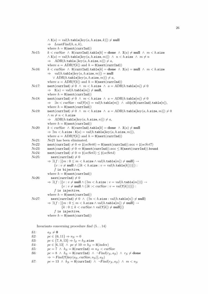
∧ X(a) = val(h.table[key(a, h.size, k)]) 6= null⇒ LeastFind(h, a, k),where h = H(next(currInd))

Ne15: k < curSize ∧ H(currInd).table[k] = done ∧ X(a) 6= null ∧ m < h.size∧ X(a) = val(h.table[key(a, h.size,m)]) ∧ n < h.size ∧ m 6= n⇒ ADR(h.table.[key(a, h.size, n)]) 6= a,where a = ADR(Y[k]) and h = H(next(currInd))

Ne16: k < curSize ∧ H(currInd).table[k] = done ∧ X(a) = null ∧ m < h.size⇒ val(h.table[key(a, h.size,m)]) = null

∨ ADR(h.table[key(a, h.size,m)]) 6= a,where a = ADR(Y[k]) and h = H(next(currInd))

Ne17: next(currInd) 6= 0 ∧ m < h.size ∧ a = ADR(h.table[m]) 6= 0⇒ X(a) = val(h.table[m]) 6= null,where h = H(next(currInd))

Ne18: next(currInd) 6= 0 ∧ m < h.size ∧ a = ADR(h.table[m]) 6= 0⇒ ∃n < curSize : val(Y[n]) = val(h.table[m]) ∧ oldp(H(currInd).table[n]),where h = H(next(currInd))

Ne19: next(currInd) 6= 0 ∧ m < h.size ∧ a = ADR(h.table[key(a, h.size,m)]) 6= 0∧ m 6= n < h.size⇒ ADR(h.table[key(a, h.size, n)]) 6= a,where h = H(next(currInd))

Ne20: k < curSize ∧ H(currInd).table[k] = done ∧ X(a) 6= null⇒ ∃m < h.size : X(a) = val(h.table[key(a, h.size,m)]),where a = ADR(Y[k]) and h = H(next(currInd))

Ne21: Ne21 has been eliminated.Ne22: next(currInd) 6= 0 ⇒ ](ocSet6) = H(next(currInd)).occ + ](ocSet7)Ne23: next(currInd) 6= 0 ⇒ H(next(currInd)).occ ≤ H(next(currInd)).boundNe24: next(currInd) 6= 0 ⇒ ](ocSet5) ≤ ](ocSet4)Ne25: next(currInd) 6= 0

⇒ ∃(f : [{m : 0 ≤ m < h.size ∧ val(h.table[m]) 6= null} →{v : v 6= null ∧ (∃k < h.size : v = val(h.table[k]))}]) :f is bijective,

where h = H(next(currInd))Ne26: next(currInd) 6= 0

⇒ ∃(f : [{v : v 6= null ∧ (∃m < h.size : v = val(h.table[m]))} →{v : v 6= null ∧ (∃k :< curSize : v = val(Y[k]))}]) :

f is injective,where h = H(next(currInd))

Ne27: next(currInd) 6= 0 ∧ (∃n < h.size : val(h.table[n]) 6= null)⇒ ∃(f : [{m : 0 ≤ m < h.size ∧ val(h.table[m]) 6= null} →

{k : 0 ≤ k < curSize ∧ val(Y[k]) 6= null}])f is injective,

where h = H(next(currInd))

Invariants concerning procedure find (5. . . 14)

fi1: afi 6= 0fi2: pc ∈ {6, 11} ⇒ nfi = 0fi3: pc ∈ {7, 8, 13} ⇒ lfi = hfi .sizefi4: pc ∈ [6, 13] ∧ pc 6= 10 ⇒ hfi = H(index)fi5: pc = 7 ∧ hfi = H(currInd) ⇒ nfi < curSizefi6: pc = 8 ∧ hfi = H(currInd) ∧ ¬Find(rfi , afi) ∧ rfi 6= done

⇒ ¬ Find(Y[key(afi , curSize, nfi)], afi)fi7: pc = 13 ∧ hfi = H(currInd) ∧ ¬Find(rfi , afi) ∧ m < nfi

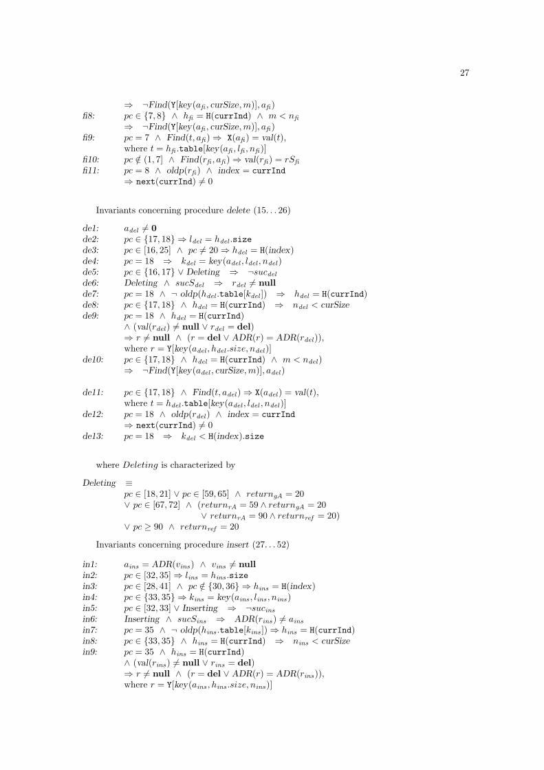
27

⇒ ¬Find(Y[key(afi , curSize,m)], afi)fi8: pc ∈ {7, 8} ∧ hfi = H(currInd) ∧ m < nfi

⇒ ¬Find(Y[key(afi , curSize,m)], afi)fi9: pc = 7 ∧ Find(t, afi) ⇒ X(afi) = val(t),

where t = hfi .table[key(afi , lfi , nfi)]fi10: pc /∈ (1, 7] ∧ Find(rfi , afi) ⇒ val(rfi) = rSfi

fi11: pc = 8 ∧ oldp(rfi) ∧ index = currInd⇒ next(currInd) 6= 0

Invariants concerning procedure delete (15. . . 26)

de1: adel 6= 0de2: pc ∈ {17, 18} ⇒ ldel = hdel .sizede3: pc ∈ [16, 25] ∧ pc 6= 20 ⇒ hdel = H(index)de4: pc = 18 ⇒ kdel = key(adel , ldel , ndel)de5: pc ∈ {16, 17} ∨ Deleting ⇒ ¬sucdelde6: Deleting ∧ sucSdel ⇒ rdel 6= nullde7: pc = 18 ∧ ¬ oldp(hdel .table[kdel ]) ⇒ hdel = H(currInd)de8: pc ∈ {17, 18} ∧ hdel = H(currInd) ⇒ ndel < curSizede9: pc = 18 ∧ hdel = H(currInd)

∧ (val(rdel) 6= null ∨ rdel = del)⇒ r 6= null ∧ (r = del ∨ ADR(r) = ADR(rdel)),where r = Y[key(adel , hdel .size, ndel)]

de10: pc ∈ {17, 18} ∧ hdel = H(currInd) ∧ m < ndel)⇒ ¬Find(Y[key(adel , curSize,m)], adel)

de11: pc ∈ {17, 18} ∧ Find(t, adel) ⇒ X(adel) = val(t),where t = hdel .table[key(adel , ldel , ndel)]

de12: pc = 18 ∧ oldp(rdel) ∧ index = currInd⇒ next(currInd) 6= 0

de13: pc = 18 ⇒ kdel < H(index).size

where Deleting is characterized by

Deleting ≡pc ∈ [18, 21] ∨ pc ∈ [59, 65] ∧ returngA = 20∨ pc ∈ [67, 72] ∧ (returnrA = 59 ∧ returngA = 20

∨ returnrA = 90 ∧ returnref = 20)∨ pc ≥ 90 ∧ returnref = 20

Invariants concerning procedure insert (27. . . 52)

in1: ains = ADR(vins) ∧ vins 6= nullin2: pc ∈ [32, 35] ⇒ lins = hins .sizein3: pc ∈ [28, 41] ∧ pc /∈ {30, 36} ⇒ hins = H(index)in4: pc ∈ {33, 35} ⇒ kins = key(ains , lins , nins)in5: pc ∈ [32, 33] ∨ Inserting ⇒ ¬sucins

in6: Inserting ∧ sucSins ⇒ ADR(rins) 6= ains

in7: pc = 35 ∧ ¬ oldp(hins .table[kins ]) ⇒ hins = H(currInd)in8: pc ∈ {33, 35} ∧ hins = H(currInd) ⇒ nins < curSizein9: pc = 35 ∧ hins = H(currInd)

∧ (val(rins) 6= null ∨ rins = del)⇒ r 6= null ∧ (r = del ∨ ADR(r) = ADR(rins)),where r = Y[key(ains , hins .size, nins)]

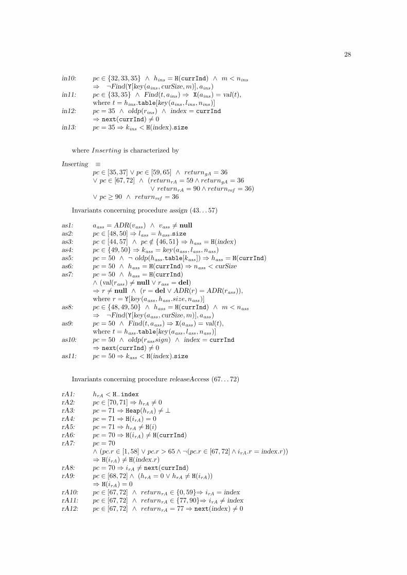
28

in10: pc ∈ {32, 33, 35} ∧ hins = H(currInd) ∧ m < nins

⇒ ¬Find(Y[key(ains , curSize,m)], ains)in11: pc ∈ {33, 35} ∧ Find(t, ains) ⇒ X(ains) = val(t),

where t = hins .table[key(ains , lins , nins)]in12: pc = 35 ∧ oldp(rins) ∧ index = currInd

⇒ next(currInd) 6= 0in13: pc = 35 ⇒ kins < H(index).size

where Inserting is characterized by

Inserting ≡pc ∈ [35, 37] ∨ pc ∈ [59, 65] ∧ returngA = 36∨ pc ∈ [67, 72] ∧ (returnrA = 59 ∧ returngA = 36

∨ returnrA = 90 ∧ returnref = 36)∨ pc ≥ 90 ∧ returnref = 36

Invariants concerning procedure assign (43. . . 57)

as1: aass = ADR(vass) ∧ vass 6= nullas2: pc ∈ [48, 50] ⇒ lass = hass .sizeas3: pc ∈ [44, 57] ∧ pc /∈ {46, 51} ⇒ hass = H(index)as4: pc ∈ {49, 50} ⇒ kass = key(aass , lass , nass)as5: pc = 50 ∧ ¬ oldp(hass .table[kass ]) ⇒ hass = H(currInd)as6: pc = 50 ∧ hass = H(currInd) ⇒ nass < curSizeas7: pc = 50 ∧ hass = H(currInd)

∧ (val(rass) 6= null ∨ rass = del)⇒ r 6= null ∧ (r = del ∨ ADR(r) = ADR(rass)),where r = Y[key(aass , hass .size, nass)]

as8: pc ∈ {48, 49, 50} ∧ hass = H(currInd) ∧ m < nass

⇒ ¬Find(Y[key(aass , curSize,m)], aass)as9: pc = 50 ∧ Find(t, aass) ⇒ X(aass) = val(t),

where t = hass .table[key(aass , lass , nass)]as10: pc = 50 ∧ oldp(rasssign) ∧ index = currInd

⇒ next(currInd) 6= 0as11: pc = 50 ⇒ kass < H(index).size

Invariants concerning procedure releaseAccess (67. . . 72)

rA1: hrA < H−indexrA2: pc ∈ [70, 71] ⇒ hrA 6= 0rA3: pc = 71 ⇒ Heap(hrA) 6= ⊥rA4: pc = 71 ⇒ H(irA) = 0rA5: pc = 71 ⇒ hrA 6= H(i)rA6: pc = 70 ⇒ H(irA) 6= H(currInd)rA7: pc = 70

∧ (pc.r ∈ [1, 58] ∨ pc.r > 65 ∧ ¬(pc.r ∈ [67, 72] ∧ irA.r = index.r))⇒ H(irA) 6= H(index.r)

rA8: pc = 70 ⇒ irA 6= next(currInd)rA9: pc ∈ [68, 72] ∧ (hrA = 0 ∨ hrA 6= H(irA))

⇒ H(irA) = 0rA10: pc ∈ [67, 72] ∧ returnrA ∈ {0, 59}⇒ irA = indexrA11: pc ∈ [67, 72] ∧ returnrA ∈ {77, 90}⇒ irA 6= indexrA12: pc ∈ [67, 72] ∧ returnrA = 77 ⇒ next(index) 6= 0

29

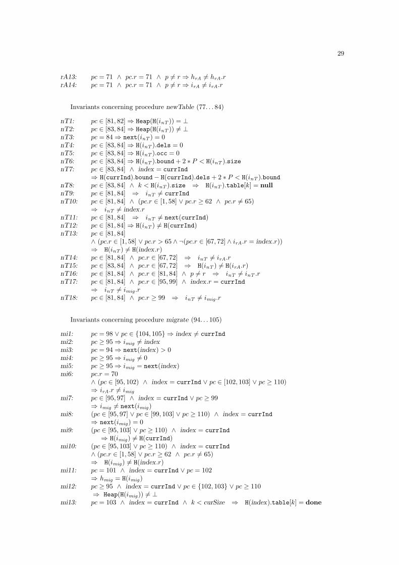
rA13: pc = 71 ∧ pc.r = 71 ∧ p 6= r ⇒ hrA 6= hrA.rrA14: pc = 71 ∧ pc.r = 71 ∧ p 6= r ⇒ irA 6= irA.r

Invariants concerning procedure newTable (77. . . 84)

nT1: pc ∈ [81, 82] ⇒ Heap(H(inT )) = ⊥nT2: pc ∈ [83, 84] ⇒ Heap(H(inT )) 6= ⊥nT3: pc = 84 ⇒ next(inT ) = 0nT4: pc ∈ [83, 84] ⇒ H(inT ).dels = 0nT5: pc ∈ [83, 84] ⇒ H(inT ).occ = 0nT6: pc ∈ [83, 84] ⇒ H(inT ).bound + 2 ∗ P < H(inT ).sizenT7: pc ∈ [83, 84] ∧ index = currInd

⇒ H(currInd).bound− H(currInd).dels + 2 ∗ P < H(inT ).boundnT8: pc ∈ [83, 84] ∧ k < H(inT ).size ⇒ H(inT ).table[k] = nullnT9: pc ∈ [81, 84] ⇒ inT 6= currIndnT10: pc ∈ [81, 84] ∧ (pc.r ∈ [1, 58] ∨ pc.r ≥ 62 ∧ pc.r 6= 65)

⇒ inT 6= index.rnT11: pc ∈ [81, 84] ⇒ inT 6= next(currInd)nT12: pc ∈ [81, 84] ⇒ H(inT ) 6= H(currInd)nT13: pc ∈ [81, 84]

∧ (pc.r ∈ [1, 58] ∨ pc.r > 65 ∧ ¬(pc.r ∈ [67, 72] ∧ irA.r = index.r))⇒ H(inT ) 6= H(index.r)

nT14: pc ∈ [81, 84] ∧ pc.r ∈ [67, 72] ⇒ inT 6= irA.rnT15: pc ∈ [83, 84] ∧ pc.r ∈ [67, 72] ⇒ H(inT ) 6= H(irA.r)nT16: pc ∈ [81, 84] ∧ pc.r ∈ [81, 84] ∧ p 6= r ⇒ inT 6= inT .rnT17: pc ∈ [81, 84] ∧ pc.r ∈ [95, 99] ∧ index.r = currInd

⇒ inT 6= imig .rnT18: pc ∈ [81, 84] ∧ pc.r ≥ 99 ⇒ inT 6= imig .r

Invariants concerning procedure migrate (94. . . 105)

mi1: pc = 98 ∨ pc ∈ {104, 105} ⇒ index 6= currIndmi2: pc ≥ 95 ⇒ imig 6= indexmi3: pc = 94 ⇒ next(index) > 0mi4: pc ≥ 95 ⇒ imig 6= 0mi5: pc ≥ 95 ⇒ imig = next(index)mi6: pc.r = 70

∧ (pc ∈ [95, 102) ∧ index = currInd ∨ pc ∈ [102, 103] ∨ pc ≥ 110)⇒ irA.r 6= imig

mi7: pc ∈ [95, 97] ∧ index = currInd ∨ pc ≥ 99⇒ imig 6= next(imig)

mi8: (pc ∈ [95, 97] ∨ pc ∈ [99, 103] ∨ pc ≥ 110) ∧ index = currInd⇒ next(imig) = 0

mi9: (pc ∈ [95, 103] ∨ pc ≥ 110) ∧ index = currInd⇒ H(imig) 6= H(currInd)

mi10: (pc ∈ [95, 103] ∨ pc ≥ 110) ∧ index = currInd∧ (pc.r ∈ [1, 58] ∨ pc.r ≥ 62 ∧ pc.r 6= 65)⇒ H(imig) 6= H(index.r)

mi11: pc = 101 ∧ index = currInd ∨ pc = 102⇒ hmig = H(imig)

mi12: pc ≥ 95 ∧ index = currInd ∨ pc ∈ {102, 103} ∨ pc ≥ 110⇒ Heap(H(imig)) 6= ⊥

mi13: pc = 103 ∧ index = currInd ∧ k < curSize ⇒ H(index).table[k] = done

30

mi14: pc = 103 ∧ index = currInd ∧ n < H(imig).size∧ LeastFind(H(imig), a, n)⇒ X(a) = val(H(imig)[key(a, H(imig).size, n)])

mi15: pc = 103 ∧ index = currInd ∧ n < H(imig).size∧ X(a) = val(H(imig).table[key(a, H(imig).size, n)] 6= null⇒ LeastFind(H(imig), a, n)

mi16: pc = 103 ∧ index = currInd ∧ k < H(imig).size⇒ ¬oldp(H(imig).table[k])

mi17: pc = 103 ∧ index = currInd ∧ X(a) 6= null ∧ k < h.size∧ X(a) = val(h.table[key(a, h.size, k)]) ∧ k 6= n < h.size⇒ ADR(h.table.[key(a, h.size, n)]) 6= a,where h = H(imig)

mi18: pc = 103 ∧ index = currInd ∧ X(a) = null ∧ k < h.size⇒ val(h.table[key(a, h.size, k)]) = null∨ ADR(h.table[key(a, h.size, k)]) 6= a,where h = H(imig)

mi19: pc = 103 ∧ index = currInd ∧ X(a) 6= null⇒ ∃m < h.size : X(a) = val(h.table[key(a, h.size,m)],where h = H(imig)

mi20: pc = 117 ∧ X(a) 6= null ∧ val(H(index).table[imC ]) 6= null∨ pc ≥ 126 ∧ X(a) 6= null ∧ index = currInd∨ pc = 125 ∧ X(a) 6= null ∧ index = currInd∧ (bmE ∨ val(wmE ) 6= null

∧ amE = ADR(wmE ))⇒ ∃m < h.size : X(a) = val(h.table[key(a, h.size,m)]),where a = ADR(Y[imC ]) and h = H(next(currInd))

Invariants concerning procedure moveContents (110. . . 118):

mC1: pc = 103 ∨ pc ≥ 110 ⇒ to = H(imig)mC2: pc ≥ 110 ⇒ from = H(index)mC3: pc > 102 ∧ m ∈ toBeMoved⇒ m < H(index).sizemC4: pc = 111 ⇒ ∃m < from.size : m ∈ toBeMovedmC5: pc ≥ 114 ∧ pc 6= 118 ⇒ vmC 6= donemC6: pc ≥ 114 ⇒ imC < H(index).sizemC7: pc = 118 ⇒ H(index).table[imC ] = donemC8: pc ≥ 110 ∧ k < H(index).size ∧ k /∈ toBeMoved

⇒ H(index).table[k] = donemC9: pc ≥ 110 ∧ index = currInd ∧ toBeMoved = ∅ ∧ k < H(index).size

⇒ H(index).table[k] = donemC10: pc ≥ 116 ∧ val(vmC ) 6= null

∧ H(index).table[imC ] = done⇒ H(imig).table[key(a, H(imig).size, 0)] 6= null,where a = ADR(vmC )

mC11: pc ≥ 116 ∧ H(index).table[imC ] 6= done⇒ val(vmC ) = val(H(index).table[imC ])∧ oldp(H(index).table[imC ])

mC12: pc ≥ 116 ∧ index = currInd ∧ val(vmC ) 6= null⇒ val(vmC ) = val(Y[imC ])

Invariants concerning procedure moveElement (120. . . 126):

mE1: pc ≥ 120 ⇒ val(vmC ) = vmE

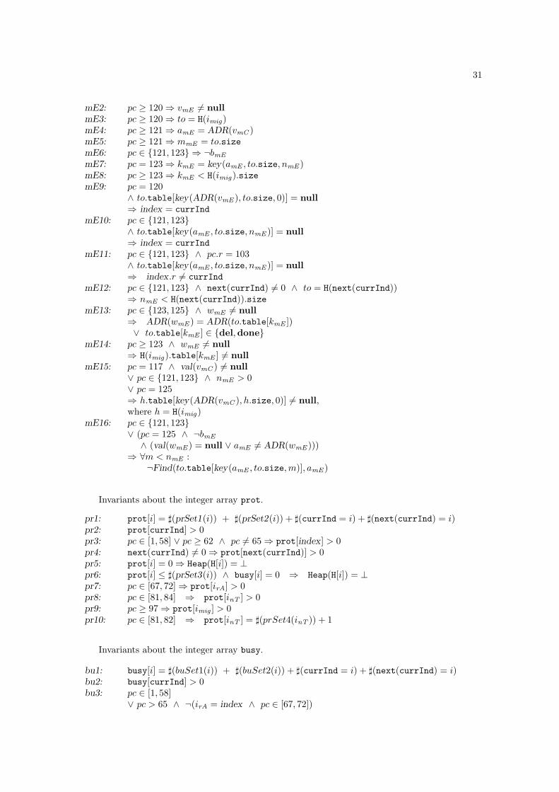
31

mE2: pc ≥ 120 ⇒ vmE 6= nullmE3: pc ≥ 120 ⇒ to = H(imig)mE4: pc ≥ 121 ⇒ amE = ADR(vmC )mE5: pc ≥ 121 ⇒ mmE = to.sizemE6: pc ∈ {121, 123} ⇒ ¬bmE

mE7: pc = 123 ⇒ kmE = key(amE , to.size, nmE )mE8: pc ≥ 123 ⇒ kmE < H(imig).sizemE9: pc = 120

∧ to.table[key(ADR(vmE ), to.size, 0)] = null⇒ index = currInd

mE10: pc ∈ {121, 123}∧ to.table[key(amE , to.size, nmE )] = null⇒ index = currInd

mE11: pc ∈ {121, 123} ∧ pc.r = 103∧ to.table[key(amE , to.size, nmE )] = null⇒ index.r 6= currInd

mE12: pc ∈ {121, 123} ∧ next(currInd) 6= 0 ∧ to = H(next(currInd))⇒ nmE < H(next(currInd)).size

mE13: pc ∈ {123, 125} ∧ wmE 6= null⇒ ADR(wmE ) = ADR(to.table[kmE ])∨ to.table[kmE ] ∈ {del,done}

mE14: pc ≥ 123 ∧ wmE 6= null⇒ H(imig).table[kmE ] 6= null

mE15: pc = 117 ∧ val(vmC ) 6= null∨ pc ∈ {121, 123} ∧ nmE > 0∨ pc = 125⇒ h.table[key(ADR(vmC ), h.size, 0)] 6= null,where h = H(imig)

mE16: pc ∈ {121, 123}∨ (pc = 125 ∧ ¬bmE

∧ (val(wmE ) = null ∨ amE 6= ADR(wmE )))⇒ ∀m < nmE :

¬Find(to.table[key(amE , to.size,m)], amE )

Invariants about the integer array prot.

pr1: prot[i] = ](prSet1(i)) + ](prSet2(i)) + ](currInd = i) + ](next(currInd) = i)pr2: prot[currInd] > 0pr3: pc ∈ [1, 58] ∨ pc ≥ 62 ∧ pc 6= 65 ⇒ prot[index] > 0pr4: next(currInd) 6= 0 ⇒ prot[next(currInd)] > 0pr5: prot[i] = 0 ⇒ Heap(H[i]) = ⊥pr6: prot[i] ≤ ](prSet3(i)) ∧ busy[i] = 0 ⇒ Heap(H[i]) = ⊥pr7: pc ∈ [67, 72] ⇒ prot[irA] > 0pr8: pc ∈ [81, 84] ⇒ prot[inT ] > 0pr9: pc ≥ 97 ⇒ prot[imig ] > 0pr10: pc ∈ [81, 82] ⇒ prot[inT ] = ](prSet4(inT )) + 1

Invariants about the integer array busy.

bu1: busy[i] = ](buSet1(i)) + ](buSet2(i)) + ](currInd = i) + ](next(currInd) = i)bu2: busy[currInd] > 0bu3: pc ∈ [1, 58]

∨ pc > 65 ∧ ¬(irA = index ∧ pc ∈ [67, 72])

32

⇒ busy[index] > 0bu4: next(currInd) 6= 0 ⇒ busy[next(currInd)] > 0bu5: pc = 81 ⇒ busy[inT ] = 0bu6: pc ≥ 100 ⇒ busy[imig ] > 0

Some other invariants we have postulated:

Ot1: X(0) = nullOt2: X(a) 6= null ⇒ ADR(X(a)) = a

The motivation of invariant (Ot1) is we never store a value for the address 0. The motivation ofinvariant (Ot2) is that the address in the hashtable is unique.

Ot3: returngA = {1, 10, 20, 30, 36, 46, 51} ∧ returnrA = {0, 59, 77, 90}∧ returnref = {10, 20, 30, 36, 46, 51} ∧ returnnT = {30, 46}

Ot4: pc ∈ {0, 1, 5, 6, 7, 8, 10, 11, 13, 14, 15, 16, 17, 18, 20,21, 25, 26, 27, 28, 30, 31, 32, 33, 35, 36, 37, 41,42, 43, 44, 46, 47, 48, 49, 50, 51, 52, 57, 59, 60,61, 62, 63, 65, 67, 68, 69, 70, 71, 72, 77, 78, 81,82, 83, 84, 90, 94, 95, 97, 98, 99, 100, 101, 102,103, 104, 105, 110, 111, 114, 116, 117, 118, 120,121, 123, 125, 126}

B Dependencies between invariants

Let us write “ϕ from ψ1, · · · , ψn” to denote that ϕ can be proved to be an invariant usingψ1, · · · , ψn hold. We write “ϕ ⇐ ψ1, · · · , ψn” to denote that ϕ can be directly derived fromψ1, · · · , ψn. We have verified the following “from” and “⇐” relations mechanically:

Co1 from fi10, Ot3, fi1Co2 from de5, Ot3, de6, del, de11Co3 from in5, Ot3, in6, in1, in11Cn1 from Cn6, Ot3Cn2 from Cn8, Ot3, delCn3 from Cn10, Ot3, in1, in5Cn4 from Cn11, Ot3No1 ⇐ No2No2 from nT1, He2, rA2, Ot3, Ha2, Ha1, rA1, rA14, rA3, nT14, rA4He1 from Ha1He2 from Ha3, rA5, Ha1, He1, rA2He3, He4 from Ot3, rA6, rA7, mi12, rA11, rA5He5 from He1He6 from rA8, Ha3, mi8, nT2, rA5Ha1 from trueHa2 from Ha1Ha3 from Ha2, Ha1, He2, He1Ha4 ⇐ Ha3, He3, He4Cn5 from Cn6, Ot3Cn6 from Cn5, Ot3Cn7 from Cn8, Ot3, delCn8 from Cn7, Ot3Cn9 from Cn10, Ot3, in1, in5

33

Cn10 from Cn9, Ot3, in5Cn11 from Cn11, Ot3Cu1 from Ot3, Ha4, rA6, rA7, nT13, nT12, Ha2, He3, He4, rA11, nT9, nT10, mi13, rA5Cu2 ⇐ Cu6, cu7, Cu3, He3, He4Cu3 from rA6, rA7, nT13, nT12, mi5, mi4, Ne8, rA5Cu4 from del, in1, as1, rA6, rA7, Ha2, nT13, nT12, Ne9, Cu9, Cu10, de7, in7, as5, He3,

He4, mi5, mi4, Ot3, Ha4, de3, mi9,mi10, de5, rA5Cu6 from Ot3, rA6, rA7, Ha2, nT13, nT12, Ha3, in3, as3, Ne23, mi5, mE6, mE7, mE10,

mE3, Ne3, mi1, mi4, rA5Cu7 from Ot3, rA6, rA7, Ha2, nT13, nT12, Ha3, in3, as3, in5, mi5, mE6, mE7, mE10, mE3,

Ne3, mi4, de7, in7, as5, Ne22, mi9,mi10, rA5, He3, mi12, mi1, Cu9, de1 in1, as1Cu8 from Cu8, FT, Ha2, nT9, nT10, rA6, rA7, mi5, mi4 , mC2, mC5, He3, He4, Cu1, Ha4,

mC6, mi16, rA5Cu9,Cu10 from rA6, rA7, nT13, nT12, Ha2, He3, He4, Cu1, Ha4, de3, in3, as3, mE3, mi9,

mi10, mE10, mE7, rA5Cu11, Cu12 from Cu9, Cu10, Cu13, Cu14, del, in1, as1, rA6, rA7, Ha2, nT13, nT12, He3,

He4, Cu1, Ha4, in3, as3, mi14, mi15, de3, in10, as8, mi12, Ot2, fi5, de8, in8, as6, Cu15,de11, in11, rA5

Cu13, Cu14 from He3, He4, Ot2, del, in1, as1, Ot1, rA6, rA7, nT13, nT12, Ha2, Cu9, Cu10,Cu1, Ha4, de3, in3, as3, Cu11, Cu12, in10, as8, fi5, de8, in8, as6, Cu15, mi17, mi18,mi12, mi4, de11, rA5

Cu15 from He3, He4, rA6, rA7, nT13, nT12, Ha2, Cu1, Ha4, del, in1, as1, de3, in3, as3, fi5,de8, in8, as6, mi12, mi19, mi4, Ot2, Cu9, Cu10, Cu11, Cu12, Cu13, Cu14, rA5

Cu16 ⇐ Cu13, Cu14, Cu15, He3, He4, Ot1Ne1 from nT9, nT10, mi7Ne2 from Ne5, nT3, mi8, nT9, nT10Ne3 from Ne1, nT9, nT10, mi8Ne4 from Ne1, nT9, nT10Ne5 from Ot3, nT9, nT10, mi5Ne6 ⇐ Ne10, Ne24, He6, He3, He4, Cu4Ne7 from Ha3, rA6, rA7, rA8, nT13, nT12, nT11, He3, He4, mi8, nT7, Ne5, Ha2, He6, rA5Ne8 from Ha3, rA8, nT11, T, mi8, nT6, Ne5, rA5Ne9 from Ha3, Ha2, Ne3, Ne5, de3, as3, rA8, rA6, rA7, nT8, nT11, mC2, nT4, mi8, rA5Ne9a from Ha3, Ne3, rA5, de3, rA8, nT4, mi8Ne10 from Ha3, Ha2, de3, rA8, nT11, Ne3, He6, mi8, nT8, mC2, nT2, Ne5, rA5Ne11 from Ha3, Ha2, He6, T, nT2, nT8, rA8, nT11, mi8, Ne3, mC2, rA5Ne12, Ne13 from Ha3, Ha2, Cu8, He6, He3, He4, Cu1, de3, in3, as3, rA8, rA6, rA7, nT11,

nT13, nT12, mi12, mi16, mi5, mi4, de7, in7, as5, Ot2, del,in1, as1, Cu9, Cu10, Cu13,Cu14, Cu15, as9, fi5, de8, in8, as6, mC2, Ne3, Ot1, Ne14, Ne20, mE16, mE7, mE4, mE1,mE12, mE2, Ne15, Ne16, Ne17, Ne18, mi20, de11, in11, rA5

Ne14 from Ha3, Ha2, He6, He3, He4, T, nT2, nT8, de3, in3, as3, rA8, nT11, Ot2, del, in1,as1, Cu9, Cu10, mi8, Ne3, mC2, mE7, mE16, mE1, mE4, mE12, Ne17, Ne18, Cu1, rA5

Ne15, Ne16 from Ha3, Ha2, Cu8, He6, He3, He4, Cu1, de3, in3, as3, rA8, rA6, rA7, nT11,nT13, nT12, mi12, mi16, mi5, mi4, de7, in7, as5, Ot2, del, in1, as1, Cu9, Cu10, Cu13,Cu14, Cu15, as9, fi5, de8, in8, as6, mC2, Ne3, Ot1, Ne19, Ne20, Ne12, Ne13, mE16, mE7,mE4, mE1, mE12, mE10, mE2, in11, de11, rA5

Ne17, Ne18 from Ha3, Ha2, mi8, He6, He3, He4, Cu1, nT2, de3, in3, as3, rA8, rA6, rA7,nT11, nT13, nT12, de7, in7, as5, Ot2, del, in1, as1, Cu9, Cu10, T, nT8, mE2, fi5, de8,in8, as6, mC2, Ne3, mC11, mC6, mC12, mE7, mE10, mE1, Cu8, Cu15, Cu13, Cu14,Cu11, Cu12, as8, de11, rA5

Ne19 from Ha3, Ha2, He6, nT2, nT8, de3, in3, as3, rA8, nT11, mi8, Ne3, mE7, Ne14, mE16,Ot1, mE1, mE4, mE12, Ne17, Ne18, rA5

Ne20 from Ha3, Ha2, Cu8, He6, He3, He4, Cu1, Ha4, de3, in3, as3, rA8, rA6, rA7, nT11,nT13, nT12, mi12, mi16, mi5, mi4, Ne1, de7, in7, as5, del, in1, as1, Cu9, Cu10, Cu13,

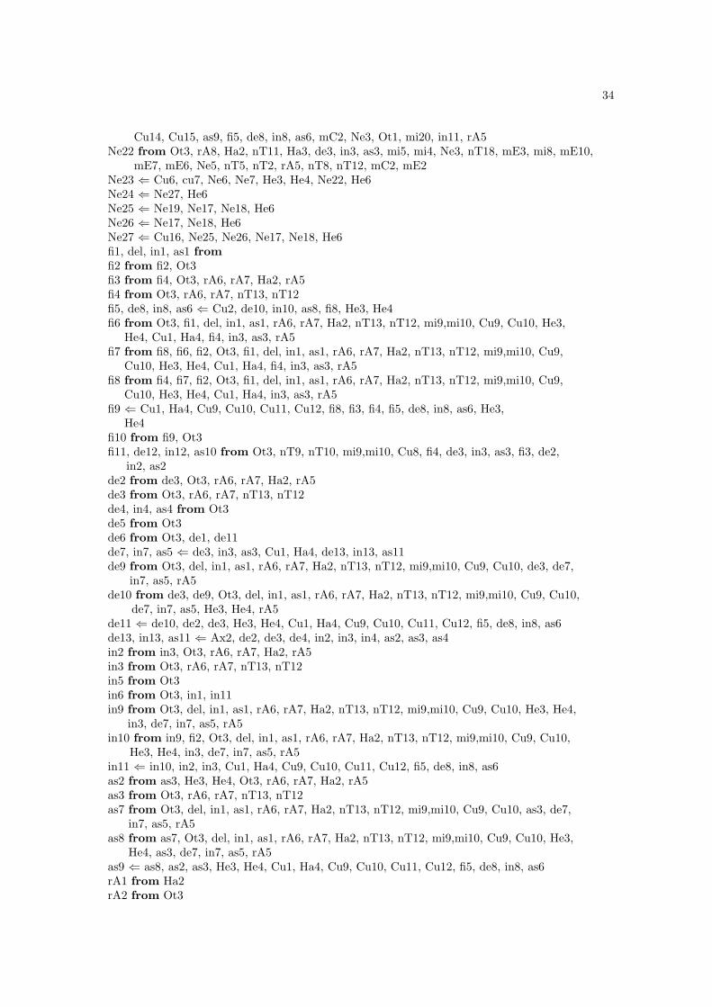
34

Cu14, Cu15, as9, fi5, de8, in8, as6, mC2, Ne3, Ot1, mi20, in11, rA5Ne22 from Ot3, rA8, Ha2, nT11, Ha3, de3, in3, as3, mi5, mi4, Ne3, nT18, mE3, mi8, mE10,

mE7, mE6, Ne5, nT5, nT2, rA5, nT8, nT12, mC2, mE2Ne23 ⇐ Cu6, cu7, Ne6, Ne7, He3, He4, Ne22, He6Ne24 ⇐ Ne27, He6Ne25 ⇐ Ne19, Ne17, Ne18, He6Ne26 ⇐ Ne17, Ne18, He6Ne27 ⇐ Cu16, Ne25, Ne26, Ne17, Ne18, He6fi1, del, in1, as1 fromfi2 from fi2, Ot3fi3 from fi4, Ot3, rA6, rA7, Ha2, rA5fi4 from Ot3, rA6, rA7, nT13, nT12fi5, de8, in8, as6 ⇐ Cu2, de10, in10, as8, fi8, He3, He4fi6 from Ot3, fi1, del, in1, as1, rA6, rA7, Ha2, nT13, nT12, mi9,mi10, Cu9, Cu10, He3,

He4, Cu1, Ha4, fi4, in3, as3, rA5fi7 from fi8, fi6, fi2, Ot3, fi1, del, in1, as1, rA6, rA7, Ha2, nT13, nT12, mi9,mi10, Cu9,

Cu10, He3, He4, Cu1, Ha4, fi4, in3, as3, rA5fi8 from fi4, fi7, fi2, Ot3, fi1, del, in1, as1, rA6, rA7, Ha2, nT13, nT12, mi9,mi10, Cu9,

Cu10, He3, He4, Cu1, Ha4, in3, as3, rA5fi9 ⇐ Cu1, Ha4, Cu9, Cu10, Cu11, Cu12, fi8, fi3, fi4, fi5, de8, in8, as6, He3,

He4fi10 from fi9, Ot3fi11, de12, in12, as10 from Ot3, nT9, nT10, mi9,mi10, Cu8, fi4, de3, in3, as3, fi3, de2,

in2, as2de2 from de3, Ot3, rA6, rA7, Ha2, rA5de3 from Ot3, rA6, rA7, nT13, nT12de4, in4, as4 from Ot3de5 from Ot3de6 from Ot3, de1, de11de7, in7, as5 ⇐ de3, in3, as3, Cu1, Ha4, de13, in13, as11de9 from Ot3, del, in1, as1, rA6, rA7, Ha2, nT13, nT12, mi9,mi10, Cu9, Cu10, de3, de7,

in7, as5, rA5de10 from de3, de9, Ot3, del, in1, as1, rA6, rA7, Ha2, nT13, nT12, mi9,mi10, Cu9, Cu10,

de7, in7, as5, He3, He4, rA5de11 ⇐ de10, de2, de3, He3, He4, Cu1, Ha4, Cu9, Cu10, Cu11, Cu12, fi5, de8, in8, as6de13, in13, as11 ⇐ Ax2, de2, de3, de4, in2, in3, in4, as2, as3, as4in2 from in3, Ot3, rA6, rA7, Ha2, rA5in3 from Ot3, rA6, rA7, nT13, nT12in5 from Ot3in6 from Ot3, in1, in11in9 from Ot3, del, in1, as1, rA6, rA7, Ha2, nT13, nT12, mi9,mi10, Cu9, Cu10, He3, He4,

in3, de7, in7, as5, rA5in10 from in9, fi2, Ot3, del, in1, as1, rA6, rA7, Ha2, nT13, nT12, mi9,mi10, Cu9, Cu10,

He3, He4, in3, de7, in7, as5, rA5in11 ⇐ in10, in2, in3, Cu1, Ha4, Cu9, Cu10, Cu11, Cu12, fi5, de8, in8, as6as2 from as3, He3, He4, Ot3, rA6, rA7, Ha2, rA5as3 from Ot3, rA6, rA7, nT13, nT12as7 from Ot3, del, in1, as1, rA6, rA7, Ha2, nT13, nT12, mi9,mi10, Cu9, Cu10, as3, de7,

in7, as5, rA5as8 from as7, Ot3, del, in1, as1, rA6, rA7, Ha2, nT13, nT12, mi9,mi10, Cu9, Cu10, He3,

He4, as3, de7, in7, as5, rA5as9 ⇐ as8, as2, as3, He3, He4, Cu1, Ha4, Cu9, Cu10, Cu11, Cu12, fi5, de8, in8, as6rA1 from Ha2rA2 from Ot3

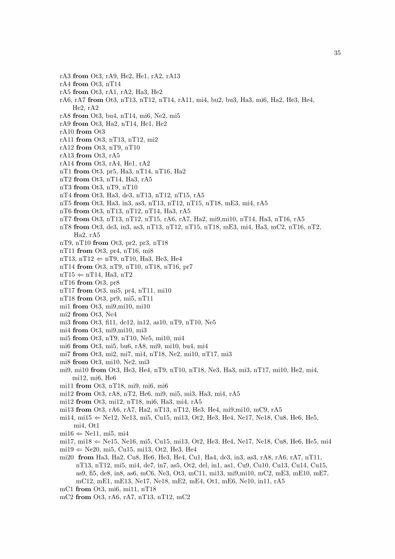
35

rA3 from Ot3, rA9, He2, He1, rA2, rA13rA4 from Ot3, nT14rA5 from Ot3, rA1, rA2, Ha3, He2rA6, rA7 from Ot3, nT13, nT12, nT14, rA11, mi4, bu2, bu3, Ha3, mi6, Ha2, He3, He4,

He2, rA2rA8 from Ot3, bu4, nT14, mi6, Ne2, mi5rA9 from Ot3, Ha2, nT14, He1, He2rA10 from Ot3rA11 from Ot3, nT13, nT12, mi2rA12 from Ot3, nT9, nT10rA13 from Ot3, rA5rA14 from Ot3, rA4, He1, rA2nT1 from Ot3, pr5, Ha3, nT14, nT16, Ha2nT2 from Ot3, nT14, Ha3, rA5nT3 from Ot3, nT9, nT10nT4 from Ot3, Ha3, de3, nT13, nT12, nT15, rA5nT5 from Ot3, Ha3, in3, as3, nT13, nT12, nT15, nT18, mE3, mi4, rA5nT6 from Ot3, nT13, nT12, nT14, Ha3, rA5nT7 from Ot3, nT13, nT12, nT15, rA6, rA7, Ha2, mi9,mi10, nT14, Ha3, nT16, rA5nT8 from Ot3, de3, in3, as3, nT13, nT12, nT15, nT18, mE3, mi4, Ha3, mC2, nT16, nT2,

Ha2, rA5nT9, nT10 from Ot3, pr2, pr3, nT18nT11 from Ot3, pr4, nT16, mi8nT13, nT12 ⇐ nT9, nT10, Ha3, He3, He4nT14 from Ot3, nT9, nT10, nT18, nT16, pr7nT15 ⇐ nT14, Ha3, nT2nT16 from Ot3, pr8nT17 from Ot3, mi5, pr4, nT11, mi10nT18 from Ot3, pr9, mi5, nT11mi1 from Ot3, mi9,mi10, mi10mi2 from Ot3, Ne4mi3 from Ot3, fi11, de12, in12, as10, nT9, nT10, Ne5mi4 from Ot3, mi9,mi10, mi3mi5 from Ot3, nT9, nT10, Ne5, mi10, mi4mi6 from Ot3, mi5, bu6, rA8, mi9, mi10, bu4, mi4mi7 from Ot3, mi2, mi7, mi4, nT18, Ne2, mi10, nT17, mi3mi8 from Ot3, mi10, Ne2, mi3mi9, mi10 from Ot3, He3, He4, nT9, nT10, nT18, Ne3, Ha3, mi3, nT17, mi10, He2, mi4,

mi12, mi6, He6mi11 from Ot3, nT18, mi9, mi6, mi6mi12 from Ot3, rA8, nT2, He6, mi9, mi5, mi3, Ha3, mi4, rA5mi12 from Ot3, mi12, nT18, mi6, Ha3, mi4, rA5mi13 from Ot3, rA6, rA7, Ha2, nT13, nT12, He3, He4, mi9,mi10, mC9, rA5mi14, mi15 ⇐ Ne12, Ne13, mi5, Cu15, mi13, Ot2, He3, He4, Ne17, Ne18, Cu8, He6, He5,

mi4, Ot1mi16 ⇐ Ne11, mi5, mi4mi17, mi18 ⇐ Ne15, Ne16, mi5, Cu15, mi13, Ot2, He3, He4, Ne17, Ne18, Cu8, He6, He5, mi4mi19 ⇐ Ne20, mi5, Cu15, mi13, Ot2, He3, He4mi20 from Ha3, Ha2, Cu8, He6, He3, He4, Cu1, Ha4, de3, in3, as3, rA8, rA6, rA7, nT11,

nT13, nT12, mi5, mi4, de7, in7, as5, Ot2, del, in1, as1, Cu9, Cu10, Cu13, Cu14, Cu15,as9, fi5, de8, in8, as6, mC6, Ne3, Ot3, mC11, mi13, mi9,mi10, mC2, mE3, mE10, mE7,mC12, mE1, mE13, Ne17, Ne18, mE2, mE4, Ot1, mE6, Ne10, in11, rA5

mC1 from Ot3, mi6, mi11, nT18mC2 from Ot3, rA6, rA7, nT13, nT12, mC2

36

mC3 from Ot3, mC3, nT13, nT12, rA6, rA7, Ha2, rA5mC4 from Ot3, mC4, mC2, mC3, He3, He4, rA6, rA7, Ha2, rA5mC5 from Ot3mC6 from Ot3, rA6, rA7, Ha2, nT13, nT12, mC2, rA5mC7 from Ot3, rA6, rA7, Ha2, nT13, nT12, mC2, rA5mC8 from Ot3, rA6, rA7, Ha2, nT13, nT12, He3, He4, mC7, rA5mC9 from Ot3, rA6, rA7, Ha2, nT13, nT12, He3, He4, mi9,mi10, He5, mC7, mC8, rA5mC10 from Ot3, rA6, rA7, Ha2, nT13, nT12, mC2, del, in1, as1, mi6, Ha3, mi4, nT18, mE15,

mC11, mi5, rA5mC11 from Ot3, rA6, rA7, Ha2, nT13, nT12, mC2, rA5mC12 from Ot3, rA6, rA7, mC2, mC11, Cu9, Cu10, de7, in7, as5, mi9, mC6mE1 from Ot3mE2 from Ot3mE3 from mC1, Ot3, mi6, nT18mE4 from Ot3, mE1mE5 from Ot3, mE3, Ha3, mi6, mi4, nT18, Ha2, rA5mE6 from Ot3mE7 from Ot3, Ha2, Ha3, mi6, mi4, mE3, rA5mE8 from Ot3, Ha3, mi6, mi4, nT18, Ha2, mE3, rA5mE9 from Cu1, Ha4, Ot3, Ha2, Ha3, mi6, mi4, mE3, mC2, mC10, mE1, mC1, del, in1, as1,

mi13, mi12, mC6, mE2, rA5mE10 from del, in1, as1, mE3, mi6, Ot3, Ha2, Ha3, mi4, mE11, mE9, mE7, rA5mE11 ⇐ mE10, mi13, mE16, mi16, mi5, mE3 , Ne12, Ne13, mC12, mE2, mE1, mE4, mC6,

mE12, mi12, Cu13, Cu14, He3, He4, mi4mE12 ⇐ Ne23, Ne22, mE16, He6, Ne8mE13 from Ot3, Ha2, mE14, del, in1, as1, Ha3, mi6, mi4, mE3, rA5mE14 from Ot3, Ha2, del, in1, as1, Ha3, mi6, mi4, nT18, mE3, mE2, rA5mE15 from Ot3, mE1, Ha2, del, in1, as1, Ha3, mi6, mi4, nT18, mE3, mE2, mE7, mE14,

mE4, rA5mE16 from Ha3, Ha2, mE3, del, in1, as1, mi6, mE2, mE4, mE1, mE7, mi4, Ot3, mE14,

mE13, rA5pr1 from Ot3, rA11, rA10, nT9, nT10, Ne5, mi2, mi4, mi8, mi5pr2, pr3 from pr1, Ot3, rA11, mi1pr4 ⇐ pr1pr5 ⇐ pr6, pr1, bu1pr6 from Ot3, Ha2, nT9, nT10, nT14, nT16, He2, rA2, pr1, bu1, pr10, rA9, He1, rA4pr7, pr8, pr9 ⇐ pr1, mi4pr10 from Ot3, pr1, nT9, nT10, nT14, nT17bu1 from Ot3, rA11, rA10, nT9, nT10, Ne5, mi2, mi8, mi5, bu5bu2, bu3 ⇐ bu1, Ot3, rA10bu4 ⇐ bu1bu5 from Ot3, nT9, nT10, nT16, nT18, pr1, bu1bu6 ⇐ bu1, mi4Ot1 from del, in1, as1Ot2 from del, in1, as1Ot3 from trueOt4 from Ot3

References

[1] Attiya, H., Bar-Noy, A., Dolev, D., Peleg, D. Reischuk, R.: Renaming in an asynchronousenvironment. J. ACM 37 (1990) 524–548

37

[2] Bar-Noy, A., Dolev, D.: Shared-memory vs. message-passing in an asynchronous distributedenvironment. In Proc. 8th ACM Symp. on principles of distributed computing, pp. 307–318,1989

[3] Cassez, F., Jard, C., Rozoy, B., Dermot, M. (Eds.): Modeling and Verification of ParallelProcesses. 4th Summer School, MOVEP 2000, Nantes, France, June 19-23, 2000.

[4] Groote, J.F., Hesselink, W.H., Mauw, S., Vermeulen, R.: An algorithm for the asynchronouswrite-all problem based on process collision. Distributed Computing 14 (2001) 75–81

[5] Harbison, S.P.: Modula-3, Prentice Hall 1992

[6] Herlihy, M.P.: Wait–free synchronization. ACM Trans. on Program. Languages and Systems13 (1991) 124–149

[7] Herlihy, M.: A methodology for implementing highly concurrent data objects. ACM Trans.on Programming Languages and Systems bf 15 (1993), 5

[8] Herlihy, M.P. and Moss, J.E.B.: Lock-free garbage collection for multiprocessors. IEEE Trans-actions on Parallel and Distributed Systems 3 304–311, 1992

[9] Hesselink, W.H.: Wait–free linearization with a mechanical proof. Distrib Comput 9 (1995)21–36

[10] Hesselink, W.H.: Bounded Delay for a Free Address. Acta Informatica 33 (1996) 233–254

[11] Hesselink, W.H., Groote, J.F.: Wait-free concurrent memory management by Create, andRead until Deletion (CaRuD). Distributed Computing 14 (2001) 31–39

[12] http://www.cs.rug.nl/~wim/mechver/hashtable

[13] Kanellakis, P.C. and Shvartsman, A.A.: Fault-tolerant parallel computation. Kluwer AcademicPublishers, 1997

[14] Lamport, L.: The temporal logic of actions. ACM Trans. on Programming Languages andSystems 16 (1994) 872–923.

[15] Knuth, D.E.: The Art of Computer Programming. Part 3, Sorting and searching. Addison-Wesley, 1973.

[16] Lynch, N.A.: Distributed Algorithms. Morgan Kaufman, San Francisco, 1996.

[17] Manna, Z., Pnueli, A.: The Temporal Logic of Reactive and Concurrent Systems: Specifica-tion. Springer-Verlag, 1992.

[18] Owre, S., Shankar, N., Rushby, J.M., Stringer-Calvert, D.W.J.: PVS Version 2.4 (2001).System Guide, Prover Guide, PVS Language Reference. http://pvs.csl.sri.com

[19] Valois, J.D.: Lock-free linked lists using compare-and-swap. Proceedings of the 14th AnnualPrinciples of Distributed Computing, pages 214-222, 1995. See also J.D. Valois. ERRATA.Lock-free linked lists using compare-and-swap. Unpublished manuscript, 1995

[20] Valois, J.D.: Implementing Lock-Free Queues, Proceedings of the Seventh International Con-ference on Parallel and Distributed Computing Systems, pages. 64-69, Las Vegas, October1994

[21] Wirth, N.: Algorithms + Data Structures = Programs. Prentice Hall, 1976.