ECE/TRANS/WP.29/2009/... - UNECE · Web viewDocument ECE-TRANS-WP29-GRPE-2014-11e was prepared by the GRPE informal working group on heavy duty hybrids (HDH), to add the test procedure

Transmitted by the HDH Secretary Informal document No. GRPE-69-1069th GRPE, 5-6 June 2014Agenda items 4(a) and 4(c)

Proposal for draft Amendment 3 to global technical regulation (gtr) No. 4: Test procedure for compression-ignition (C.I.) engines and positive-ignition (P.I.) engines fuelled with natural gas (NG) or liquefied petroleum gas (LPG) with regard to the emission of pollutants - document ECE-TRANS-WP29-GRPE-2014-11e

Amendments and complements to be taken into consideration

I. Background

Document ECE-TRANS-WP29-GRPE-2014-11e was prepared by the GRPE informal working group on heavy duty hybrids (HDH), to add the test procedure on heavy duty hybrids to gtr n° 4. In addition, minor changes of aligning gtr n° 4 with gtr n° 11 on nonroad mobile machinery are being introduced, as approved by WP.29 at its 162th session. With the agreement of GRPE, this document was due to be completed and when necessary amended in order to take into consideration the latest work progress of the HDH informal working group. This informal document presents these complements and amendments. The modifications to the original English text are marked using track changes. Non relevant editorial changes, such as section numbering and number of equations, tables and figures are not marked in all cases.

It should be noted that equations, tables and figures numbering and the corresponding references, and the symbols list in paragraph 3.2 have not yet been fully completed. This will be done during the final editing of document ECE-TRANS-WP29-GRPE-2014-11e.

1

II. Proposal

A. Statement of technical rationale and justification

Section 2., amend to read

2. Anticipated benefits

7. To enable manufacturers to develop new hybrid vehicle models more effectively and within a shorter time, it is desirable that gtr n°4 should be amended to cover the special requirements for hybrid vehicles. These savings will accrue not only to the manufacturer, but more importantly, to the consumer as well.Reserved.

However, amending a test procedure just to address the economic question does not address the mandate given when work on this amendment was first started. The test procedure must also better reflect how heavy-duty engines are are actually operated in hybrid vehicles. Compared to the measurement methods defined in this gtr, the new testing methods for hybrid vehicles are more representative of in-use driving behaviour of heavy-duty hybrid vehicles.

B. Text of Regulation


“2. Scope

2.1 This regulation applies to the measurement of the emission of gaseous and particulate pollutants from compression-ignition engines and positive-igni-tion engines fuelled with natural gas (NG) or liquefied petroleum gas (LPG), used for propelling motor vehicles, including hybrid vehicles, of categories 1-2 and 2, having a design speed exceeding 25 km/h and having a maximum mass exceeding 3.5 tonnes.

2.2. This regulation also applies to the measurement of the emission of gaseous and particulate pollutants from powertrains, used for propelling hybrid motor vehicles of categories 1-2 and 2, having a design speed exceeding 25 km/h and having a maximum mass exceeding 3.5 tonnes, being equipped with compression-ignition engines or positive-ignition engines fuelled with NG or LPG. It does not apply to plug-in hybrids.

Section 3.1.14., amend to read

3.1.14. "Energy converter" means the part of the powertrain converting one form of energy into a different one for the primary purpose of vehicle propulsion.

2


3.1.16. "Energy storage system" means the part of the powertrain that can store chemical, electrical or mechanical energy and that may also be able to internally convert those energies without being directly used for vehicle propulsion, and which can be refilled or recharged externally and/or internally.

Sections 3.1.37 and 3.1.52.,to be added

3.1.37. “Parallel hybrid” means a hybrid vehicle which is not a series hybrid; it includes power-split and series-parallel hybrids.

3.1.52. “Series hybrid” means a hybrid vehicle where the power delivered to the driven wheels is provided solely by energy converters other than the internal combustion engine.

New section 3.2.1., to be added

3.2.1 Symbols of Annexes 9 and 10

Symbol Unit Term

A, B, C - chassis dynamometer polynomial coefficients

Afront m2 vehicle frontal areaASGflg - automatic start gear detection flag

c - tuning constant for hyperbolic functionC F capacitance

CAP Ah battery coulomb capacityCcap F rated capacitance of capacitorCdrag - vehicle air drag coefficientDpm m3 hydraulic pump/motor displacement

Dtsyncindi s clutch synchronization indicationDynomeas-

ured

- chassis dynamometer A, B, C measured parameters

Dynosettings - chassis dynamometer A, B, C parameter settingDynotarget - chassis dynamometer A, B, C target parameters

e V battery open-circuit voltageEflywheel J flywheel kinetic energy

famp - torque converter mapped torque amplificationfpump Nm torque converter mapped pump torque

Froadload N chassis dynamometer road load

froll - tyre rolling resistance coefficientg m/s2 gravitational coefficient

iaux A electric auxiliary currentiem A electric machine currentJ kgm2 rotating inertia

3

Symbol Unit Term

Jaux kgm2 mechanical auxiliary load inertiaJcl,1 / Jcl,2 kgm2 clutch rotational inertias

Jem kgm2 electric machine rotational inertiaJfg kgm2 final gear rotational inertia

Jflywheel kgm2 flywheel inertiaJgear kgm2 transmission gear rotational inertia

Jp / Jt kgm2 torque converter pump / turbine rotational inertiaJpm kgm2 hydraulic pump/motor rotational inertia

Jpowertrain kgm2 total powertrain rotational inertiaJretarder kgm2 retarder rotational inertiaJspur kgm2 spur gear rotational inertiaJtot kgm2 total vehicle powertrain inertiaJwheel kgm2 wheel rotational inertiaKK - PID anti-windup parameter

KP, KI, KD - PID controller parametersMaero Nm aerodynamic drag torque

Mcl Nm clutch torqueMcl,maxtorque Nm maximum clutch torque

MCVT Nm CVT torqueMdrive Nm drive torque

Mem Nm electric machine torqueMflywheel,loss W flywheel torque loss

Mgrav Nm gravitational torqueMice Nm engine torqueM

mech,aux

Nm mechanical auxiliary load torque

Mmech_bra

ke

Nm mechanical friction brake torque

Mp / Mt Nm torque converter pump / turbine torqueMpm Nm hydraulic pump/motor torque

Mretarder Nm retarder torqueMroll Nm rolling resistance torqueMstart Nm ICE starter motor torqueMtc,loss Nm torque converter torque loss during lock-up

mvehicle kg vehicle test mass

mvehicle,0

kg vehicle curb mass

nact min-1 actual engine speed

nfinal min-1 final speed at end of testninit min-1 initial speed at start of test

4

Symbol Unit Term

ns / np - number of series / parallel cellsP kW (hybrid system) rated power

pacc Pa hydraulic accumulator pressurepedalacceler-

ator

- accelerator pedal position

pedalbrake - brake pedal positionpedalclutch - clutch pedal positionpedallimit - clutch pedal thresholdPel,aux kW electric auxiliary power

Pel,em kW electric machine electrical powerPem kW electric machine mechanical powerpgas Pa accumulator gas pressure

Pice,loss W ICE power lossPloss,bat W battery power lossPloss,em kW electric machine power loss

Pmech,aux

kW mechanical auxiliary load power

Prated kW (hybrid system) rated powerpres Pa hydraulic accumulator sump pressureQpm m3 /s hydraulic pump/motor volumetric flowRbat,th K/W battery thermal resistancerCVT - CVT ratioRem,th K/W thermal resistance for electric machinerfg - final gear ratiorgear - transmission gear ratioRi Ω capacitor internal resistance

Ri0, R Ω battery internal resistancerspur - spur gear ratio

rwheel m wheel radiusSGflg - skip gear flag

sliplimit rad/s clutch speed thresholdSOC - state-of-charge

Tact(nact) Nm actual engine torque at actual engine speedTbat K battery temperature

Tbat,cool K battery coolant temperatureTcapacitor K capacitor temperatureTclutch s clutch timeTem K electric machine temperature

Tem,cool K electric machine coolant temperatureTice,oil K ICE oil temperature

Tmax(nact) Nm maximum engine torque at actual engine speedTnorm - normalized duty cycle torque value

5

Symbol Unit Term

Tstartgear s gear shift time prior to driveawayu V voltageuC V capacitor voltageucl - clutch pedal actuation

Ufinal V final voltage at end of testuin / uout V input / output voltageUinit V initial voltage at start of testureq V requested voltage

VC,min/max V capacitor minimum / maximum voltageVgas m3 accumulator gas volume

vmax km/h maximum vehicle speedVnominal V rated nominal voltage for REESSvvehicle m/s vehicle speed

Wact kWh actual engine workWeng_HILS kWh engine work in the HILS simulated run

Weng_test

kWh engine work in chassis dynamometer test

Wsys kWh hybrid system workWsys_HILS kWh hybrid system work in the HILS simulated runWsys_test kWh hybrid system work in powertrain test

x - control signalxDCDC - DC/DC converter control signalαroad rad road gradient

γ - adiabatic indexΔAh Ah net change of REESS coulombic chargeΔE kWh net energy change of RESS

ΔEHILS kWh net energy change of RESS in HILS simulated runningΔEtest kWh net energy change of RESS in testηCVT - CVT efficiencyηDCDC - DC/DC converter efficiencyηem - electric machine efficiencyηfg - final gear efficiency

ηgear - transmission gear efficiencyηpm - hydraulic pump/motor mechanical efficiencyηspur - spur gear efficiencyηvpm - hydraulic pump/motor volumetric efficiencyρa kg/m3 air densityτ1 - first order time response constant

τbat,heat J/K battery thermal capacityτclose s clutch closing time constant

τdriveaway s clutch closing time constant for driveaway

6

Symbol Unit Term

τem,heat J/K thermal capacity for electric machine massτopen s clutch opening time constantω rad/s shaft rotational speed

ωp / ωt rad/s torque converter pump / turbine speed❑ rad/s2 rotational acceleration

Section 5.1., amend to read

5.1. Emission of gaseous and particulate pollutants

5.1.1. Internal combustion engine

The emissions of gaseous and particulate pollutants by the engine shall be determined on the WHTC and WHSC test cycles, as described in paragraph 7. This paragraph also applies to vehicles with integrated starter/generator systems where the generator is not used for propelling the vehicle, for example stop/start systems.

For hybrid vehicles, the emissions of gaseous and particulate pollutants shall be determined on the cycles derived in accordance with Annex 9 for the HEC or Annex 10 for the HPC.

5.1.2. Hybrid powertrain

The emissions of gaseous and particulate pollutants by the hybrid powertrain shall be determined on the duty cycles derived in accordance with Annex 9 for the HEC or Annex 10 for the HPC.

Hybrid powertrains may be tested in accordance with paragraph 5.1.1., if the ratio between the propelling power of the electric motor, as measured in accordance with paragraph A.9.8.4. at speeds above idle speed, and the rated power of the engine is less than or equal to 5 per cent.

5.1.2.1. The Contracting Parties may decide to not make paragraph 5.1.2. and the related provisions for hybrid vehicles, specifically Annexes 9 and 10, compulsory in their regional transposition of this gtr.

In such case, the internal combustion engine used in the hybrid powertrain shall meet the applicable requirements of paragraph 5.1.1.

5.1.3. Measurement system

The measurement systems shall meet the linearity requirements in paragraph 9.2. and the specifications in paragraph 9.3. (gaseous emissions measurement), paragraph 9.4. (particulate measurement) and in Annex 3.

Other systems or analyzers may be approved by the type approval or certification authority, if it is found that they yield equivalent results in accordance with paragraph 5.1.14

5.1.14. Equivalency


5.3.2. Special requirements

7

For a hybrid powertrain, interaction between design parameters shall be identified by the manufacturer in order to ensure that only hybrid powertrains with similar exhaust emission characteristics are included within the same hybrid powertrain family. These interactions shall be notified to the type approval or certification authority, and shall be taken into account as an additional criterion beyond the parameters listed in paragraph 5.3.3. for creating the hybrid powertrain family.

The individual test cycles HEC and HPC depend on the configuration of the hybrid powertrain. In order to determine if a hybrid powertrain belongs to the same family, or if a new hybrid powertrain configuration is to be added to an existing family, the manufacturer shall simulate a HILS test or run a powertrain test with this powertrain configuration and record the resulting duty cycle. This duty cycle shall be compared to the duty cycle of the parent hybrid powertrain and meet the criteria in paragraph 5.3.2.1.

The duty cycle torque values shall be normalized as follows:

❑❑❑❑❑❑

❑❑❑❑ (1)

Where:

Tnorm are the normalized duty cycle torque values

nact is the actual engine speed, min-1

Tact(nact) is the actual engine torque at actual engine speed, Nm

Tmax(nact) is the maximum engine torque at actual engine speed, Nm

The normalized duty cycle shall be evaluated against the normalized duty cycle of the parent hybrid powertrain by means of a linear regression analysis. This analysis shall be performed at 1 Hz or greater. A hybrid powertrain shall be deemed to belong to the same family, if the criteria of table 2 in paragraph 7.8.8. are met.

5.3.2.1. Reserved

5.3.2.21. In addition to the parameters listed in paragraph 5.3.3., the manufacturer may introduce additional criteria allowing the definition of families of more restricted size. These parameters are not necessarily parameters that have an influence on the level of emissions.

Sections 5.3.3.1., 5.3.3.2. and 5.3.3.7., amend to read

5.3.3.1. Hybrid topology (architecture)

(a) Parallel

(b) Series

5.3.3.12. Internal combustion engine

The engine family criteria of paragraph 5.2 shall be met when selecting the engine for the hybrid powertrain family.

Engines from different engine families with respect to paragraphs 5.2.3.2, 5.2.3.4, and 5.2.3.9 may be combined into a hybrid powertrain family based on their overall emission behavior.

5.3.3.2. Power of the internal combustion engine

8

Reserved

5.3.3.7. Other

Reserved.


5.3.4. Choice of the parent hybrid powertrain

Once the powertrain family has been agreed by the type approval or certification authority, the parent hybrid powertrain of the family shall be selected using the internal combustion engine with the highest power.

In case the engine with the highest power is used in multiple hybrid powertrains, the parent hybrid powertrain shall be the hybrid powertrain with the highest ratio of internal combustion engine to hybrid system work determined by HILS simulation or powertrain test.


6. TEST CONDITIONS

The general test conditions laid down in this paragraph shall apply to testing of the internal combustion engine (WHTC, WHSC, HEC) and of the powertrain (HPC) as specified in Annex 10.


...

The after-treatment system is considered to be of the continuous regeneration type if the conditions declared by the manufacturer occur during the test during a sufficient time and the emission results do not scatter by more than ±25 per cent for the gaseous components and by not more than ±25 per cent or 0.005 g/kWh, whichever is greater, for PM.


….

Average brake specific emissions between regeneration phases shall be determined from the arithmetic mean of several approximately equidistant hot start test results (g/kWh). As a minimum, at least one hot start test as close as possible prior to a regeneration test and one hot start test immediately after a regeneration test shall be conducted. As an alternative, the manufacturer may provide data to show that the emissions remain constant (25 per cent for the gaseous components and ±25 per cent or 0.005 g/kWh, whichever is greater, for PM) between regeneration phases. In this case, the emissions of only one hot start test may be used.


9

9. Equipment specification and verification

This paragraph describes the required calibrations, verifications and interfer-ence checks of the measurement systems. Calibrations or verifications shall be generally performed over the complete measurement chain.

Internationally recognized-traceable standards shall be used to meet the toler-ances specified for calibrations and verifications.

Instruments shall meet the specifications in table 7 for all ranges to be used for testing. Furthermore, any documentation received from instrument manu-facturers showing that instruments meet the specifications in table 7 shall be kept.

Table 8 summarizes the calibrations and verifications described in para-graph 9 and indicates when these have to be performed.

Overall systems for measuring pressure, temperature, and dew point shall meet the requirements in table 8 and table 9. Pressure transducers shall be located in a temperature-controlled environment, or they shall compensate for temperature changes over their expected operating range. Transducer materi-als shall be compatible with the fluid being measured.This gtr does not con-tain details of flow, pressure, and temperature measuring equipment or sys-tems. Instead, only the linearity requirements of such equipment or systems necessary for conducting an emissions test are given in paragraph 9.2.

Table 7 (new)Recommended performance specifications for measurement instruments

Measurement Instrument

Complete SystemRise time

Recordingfrequency

Accuracy Repeatability

Engine speed transducer 1 s 1 Hz means2.0 % of pt. or0.5 % of max

1.0 % of pt. or0.25 % of max

Engine torque transducer 1 s 1 Hz means2.0 % of pt. or1.0 % of max

1.0 % of pt. or0.5 % of max

Fuel flow meter 5 s 1 Hz 2.0 % of pt. or1.5 % of max

1.0 % of pt. or0.75 % of max

CVS flow(CVS with heat exchanger)

1 s(5 s)

1 Hz means(1 Hz)


1.0 % of pt. or0.75 % of max

Dilution air, inlet air, exhaust, and sample flow meters 1 s

1 Hz means of 5 Hz samples


1.25 % of pt. or0.75 % of max

Continuous gas analyzer raw 2.5 s 2 Hz2.0 % of pt. or2.0 % of meas.

1.0 % of pt. or1.0 % of meas.

Continuous gas analyzer dilute 5 s 1 Hz2.0 % of pt. or2.0 % of meas.


Batch gas analyzer N/A N/A2.0 % of pt. or2.0 % of meas.


Analytical balance N/A N/A 1.0 µg 0.5 µg

10

a)Accuracy and repeatabilit

Note: Accuracy and repeatability are based on absolute values. "pt." refers to the overall mean value expected at the respective emission limit ; "max." refers to the peak value expected at the re -spective emission limit over the duty cycle, not the maximum of the instrument's range; "meas." refers to the actual mean measured over the duty cycle.

11

Table 8 (new)Summary of Calibration and Verifications

Type of calibration or verification

Minimum frequency (a)

9.2.: linearity Speed: Upon initial installation, within 370 days before testing and after major maintenance.Torque: Upon initial installation, within 370 days before testing and after major maintenance.Clean air and diluted exhaust flows: Upon initial installation, within 370 days before testing and after major maintenance, unless flow is verified by propane check or by carbon oxygen balance.Raw exhaust flow: Upon initial installation, within 185 days before testing and after major maintenance.Gas analyzers: Upon initial installation, within 35 days before testing and after major maintenance.PM balance: Upon initial installation, within 370 days before testing and after major maintenance.Pressure and temperature: Upon initial installation, within 370 days before testing and after major maintenance.

9.3.1.2.: accuracy, repeatability and noise

Accuracy: Not required, but recommended for initial installation.Repeatability: Not required, but recommended for initial installation.Noise: Not required, but recommended for initial installation.

9.4.5.6.: flow instrument calibration

Upon initial installation and after major maintenance.

9.5.: CVS calibration Upon initial installation and after major maintenance.

9.5.5: CVS verification (b) Upon initial installation, within 35 days before testing, and after major maintenance. (propane check)

9.3.4.: vacuum-side leak check

Before each laboratory test according to paragraph 7.

9.3.9.1: CO analyzer interference check


9.3.7.1.: Adjustment of the FID

Upon initial installation and after major maintenance

9.3.7.2.: Hydrocarbon response factors

Upon initial installation, within 185 days before testing, and after major maintenance.

9.3.7.3.: Oxygen interference check

Upon initial installation, and after major maintenance and after FID optimization according to 9.3.7.1.

9.3.8.: Efficiency of the non-methane cutter (NMC)


9.3.9.2.: NOx analyzer quench check for CLD


9.3.9.3.: NOx analyzer quench check for NDUV


9.3.9.4.: Sampler dryer Upon initial installation and after major maintenance.

9.3.6.: NOx converter efficiency


12

Type of calibration or verification

Minimum frequency (a)

(a) Perform calibrations and verifications more frequently, according to measurement system manufacturer instructions and good engineering judgment.

(b) The CVS verification is not required for systems that agree within ± 2per cent based on a chemical balance of carbon or oxygen of the intake air, fuel, and diluted exhaust.


9.1. Dynamometer specification

9.1.1. Shaft work

An engine dynamometer shall be used that has adequate characteristics to perform the applicable duty cycle including the ability to meet appropriate cycle validation criteria. The following dynamometers may be used:

(a) Eddy-current or water-brake dynamometers;

(b) Alternating-current or direct-current motoring dynamometers;

(c) One or more dynamometers.

An engine dynamometer with adequate characteristics to perform the appro-priate test cycle described in paragraphs 7.2.1. and 7.2.2. shall be used.

The instrumentation for torque and speed measurement shall allow the meas-urement accuracy of the shaft power as needed to comply with the cycle val-idation criteria. Additional calculations may be necessary. The accuracy of the measuring equipment shall be such that the linearity requirements given in paragraph 9.2., Table 7 are not exceeded.

9.1.2. Torque measurement

Load cell or in-line torque meter may be used for torque measurements.

When using a load cell, the torque signal shall be transferred to the engine axis and the inertia of the dynamometer shall be considered. The actual engine torque is the torque read on the load cell plus the moment of inertia of the brake multiplied by the angular acceleration. The control system has to perform such a calculation in real time.


9.2. Linearity requirements

The calibration of all measuring instruments and systems shall be traceable to national (international) standards. The measuring instruments and systems shall comply with the linearity requirements given in Table 79. The linearity verification according to paragraph 9.2.1. shall be performed for the gas ana-lyzers within 35 days before testing at least every 3 months or whenever a system repair or change is made that could influence calibration. For the other instruments and systems, the linearity verification shall be done within

13

370 days before testingas required by internal audit procedures, by the instru-ment manufacturer or in accordance with ISO 9000 requirements.

Table 7, re-number table 9


9.3.1. Analyzer specifications

9.3.1.1. General

The analyzers shall have a measuring range and response time appropriate for the accuracy required to measure the concentrations of the exhaust gas com-ponents under transient and steady state conditions.

The electromagnetic compatibility (EMC) of the equipment shall be on a level as to minimize additional errors.

Analyzers may be used, that have compensation algorithms that are functions of other measured gaseous components, and of the fuel properties for the spe-cific engine test. Any compensation algorithm shall only provide offset com-pensation without affecting any gain (that is no bias).

9.3.1.2. Verifications for accuracy, repeatability, and noiseAccuracy

The performance values for individual instruments specified in table 7 are the basis for the determination of the accuracy, repeatability, and noise of an in-strument.

It is not required to verify instrument accuracy, repeatability, or noise. How-ever, it may be useful to consider these verifications to define a specification for a new instrument, to verify the performance of a new instrument upon de-livery, or to troubleshoot an existing instrument.The accuracy, defined as the deviation of the analyzer reading from the reference value, shall not exceed ±2 per cent of the reading or ± 0.3 per cent of full scale whichever is larger.

9.3.1.3. Precision

The precision, defined as 2.5 times the standard deviation of 10 repetitive re-sponses to a given calibration or span gas, shall be no greater than 1 per cent of full scale concentration for each range used above 155 ppm (or ppm C) or 2 per cent of each range used below 155 ppm (or ppm C).

9.3.1.4. Noise

The analyzer peak-to-peak response to zero and calibration or span gases over any 10 seconds period shall not exceed 2 per cent of full scale on all ranges used.

9.3.1.5. Zero drift

The drift of the zero response shall be specified by the instrument manufac-turer.

9.3.1.6. Span drift

The drift of the span response shall be specified by the instrument manufac-turer.

9.3.1.73. Rise time

The rise time of the analyzer installed in the measurement system shall not exceed 2.5 s.

14

9.3.1.84. Gas drying

Exhaust gases may be measured wet or dry. A gas-drying device, if used, shall have a minimal effect on the composition of the measured gases. It shall meet the requirements of section 9.3.9.4.

The following gas-drying devices are permitted:

(a) An osmotic-membrane dryer shall meet the temperature specifications in paragraph 9.3.2.2. The dew point, Tdew, and absolute pressure, ptotal, down-stream of an osmotic-membrane dryer shall be monitored.

(b) A thermal chiller shall meet the NO2 loss-performance check specified in paragraph 9.3.9.4.

Chemical dryers are not an acceptable method ofpermitted for removing wa-ter from the sample.

Section 9.3.3.3., amend to read

9.3.3.3. Gas dividers

The gases used for calibration and span may also be obtained by means of gas dividers (precision blending devices), diluting with purified N2 or with purified synthetic air. Critical-flow gas dividers, capillary-tube gas dividers, or thermal-mass-meter gas dividers may be used. Viscosity corrections shall be applied as necessary (if not done by gas divider internal software) to ap-propriately ensure correct gas division. The accuracy of the gas divider shall be such that the concentration of the blended calibration gases is accurate to within ±2 per cent. This accuracy implies that primary gases used for blend-ing shall be known to an accuracy of at least 1 per cent, traceable to na-tional or international gas standards. The verification shall be performed at between 15 and 50 per cent of full scale for each calibration incorporating a gas divider. An additional verification may be performed using another calib-ration gas, if the first verification has failed.

The gas divider system shall meet the linearity verification in paragraph 9.2., table 7. Optionally, the blending device may be checked with an instrument which by nature is linear, e.g. using NO gas with a CLD. The span value of the instrument shall be adjusted with the span gas directly connected to the instrument. The gas divider shall be checked at the settings used and the nominal value shall be compared to the measured concentration of the instru-ment. This difference shall in each point be within ±1 per cent of the nom-inal value.

For conducting the linearity verification according to paragraph 9.2.1., the gas divider shall be accurate to within 1 per cent.


9.3.4. Vacuum-side Lleak check

Upon initial sampling system installation, after major maintenance such as pre-filter changes, and within 8 hours prior to each test sequence, it shall be verified that there are no significant vacuum-side leaks using one of the leak

15

tests described in this section. This verification does not apply to any full-flow portion of a CVS dilution system.

A leak may be detected either by measuring a small amount of flow when there shall be zero flow, by measuring the pressure increase of an evacuated system, or by detecting the dilution of a known concentration of span gas when it flows through the vacuum side of a sampling system. A system leak check shall be performed.

9.3.4.1. Low-flow leak test

The probe shall be disconnected from the exhaust system and the end plugged. The analyzer pump shall be switched on. After an initial stabiliza-tion period all flowmeters will read approximately zero in the absence of a leak. If not, the sampling lines shall be checked and the fault corrected.

The maximum allowable leakage rate on the vacuum side shall be 0.5 per cent of the in-use flow rate for the portion of the system being checked. The analyzer flows and bypass flows may be used to estimate the in-use flow rates.

9.3.4.2. Vacuum-decay leak test

Alternatively, the The system may shall be evacuated to a pressure of at least 20 kPa vacuum (80 kPa absolute) and the leak rate of the system shall be ob-served as a decay in the applied vacuum. To perform this test the vacuum-side volume of the sampling system shall be known to within ±10 per cent of its true volume.

After an initial stabilization period the pressure increase p (kPa/min) in the system shall not exceed:

p = p / Vs x 0.005 x qvs (74)

Where:

Vs is the system volume, l

qvs is the system flow rate, l/min

16

9.3.4.3. Dilution-of-span-gas leak test

A gas analyzer shall be prepared as it would be for emission testing. Span gas shall be supplied to the analyzer port and it shall be verified that the span gas concentration is measured within its expected measurement accuracy and re-peatability. Overflow span gas shall be routed to either the end of the sample probe, the open end of the transfer line with the sample probe disconnected, or a three-way valve installed in-line between a probe and its transfer line. Another method is the introduction of a concentration step change at the be-ginning of the sampling line by switching from zero to span gas. If for a cor-rectly calibrated analyzer after an adequate period of time the reading is ≤ 99 per cent compared to the introduced concentration, this points to a leakage problem that shall be corrected.

It shall be verified that the measured overflow span gas concentration is within ±0.5 per cent of the span gas concentration. A measured value lower than expected indicates a leak, but a value higher than expected may indicate a problem with the span gas or the analyzer itself. A measured value higher than expected does not indicate a leak.


9.3.8. Efficiency of the non-methane cutter (NMC)

The NMC is used for the removal of the non-methane hydrocarbons from the sample gas by oxidizing all hydrocarbons except methane. Ideally, the con-version for methane is 0 per cent, and for the other hydrocarbons represented by ethane is 100 per cent. For the accurate measurement of NMHC, the two efficiencies shall be determined and used for the calculation of the NMHC emission mass flow rate (see paragraph 8.6.2.).

It is recommended that a non-methane cutter is optimized by adjusting its temperature to achieve a ECH4 < 0.15 and a EC2H6 > 0.98 as determined by paragraph 9.3.8.1. and 9.9.8.2., as applicable. If adjusting NMC temperature does not result in achieving these specifications, it is recommended that the catalyst material is replaced.

Section 9.3.9.2.3., amend to read

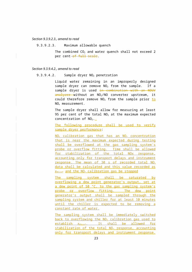
9.3.9.2.3. Maximum allowable quench

The combined CO2 and water quench shall not exceed 2 per cent of full scale.

Section 9.3.9.4.2., amend to read

9.3.9.4.2. Sample dryer NO2 penetration

Liquid water remaining in an improperly designed sample dryer can remove NO2 from the sample. If a sample dryer is used in combination with an NDUV analyzer without an NO2/NO converter upstream, it could therefore remove NO2 from the sample prior to NOx measurement.

The sample dryer shall allow for measuring at least 95 per cent of the total NO2 at the maximum expected concentration of NO2.

The following procedure shall be used to verify sample dryer performance:

17

NO2 calibration gas that has an NO2 concentration that is near the maximum expected during testing shall be overflowed at the gas sampling system's probe or overflow fitting. Time shall be allowed for stabilization of the total NOx response, accounting only for transport delays and instrument response. The mean of 30 s of recorded total NOx data shall be calculated and this value recorded as xNOxref and the NO2 calibration gas be stopped

The sampling system shall be saturated by overflowing a dew point gener-ator's output, set at a dew point of 50 °C, to the gas sampling system's probe or overflow fitting. The dew point generator's output shall be sampled through the sampling system and chiller for at least 10 minutes until the chiller is expected to be removing a constant rate of water.

The sampling system shall be immediately switched back to overflowing the NO2 calibration gas used to establish xNOxref. It shall be allowed for stabiliza-tion of the total NOx response, accounting only for transport delays and in-strument response. The mean of 30 s of recorded total NOx data shall be cal-culated and this value recorded as xNOxmeas.

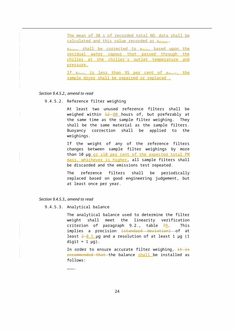
xNOxmeas shall be corrected to xNOxdry based upon the residual water vapour that passed through the chiller at the chiller's outlet temperature and pressure.

If xNOxdry is less than 95 per cent of xNOxref, the sample dryer shall be repaired or replaced .


9.4.5.2. Reference filter weighing

At least two unused reference filters shall be weighed within 12 80 hours of, but preferably at the same time as the sample filter weighing. They shall be the same material as the sample filters. Buoyancy correction shall be applied to the weighings.

If the weight of any of the reference filters changes between sample filter weighings by more than 10 µg or ±10 per cent of the expected total PM mass, whichever is higher, all sample filters shall be discarded and the emissions test repeated.

The reference filters shall be periodically replaced based on good engineering judgement, but at least once per year.


9.4.5.3. Analytical balance

The analytical balance used to determine the filter weight shall meet the lin-earity verification criterion of paragraph 9.2., table 79. This implies a preci-sion (standard deviation) of at least 2 0.5 µg and a resolution of at least 1 µg (1 digit = 1 µg).

In order to ensure accurate filter weighing, it is recommended that the bal-ance shall be installed as follows:

……….

18

Annex 1(b)., amend to read

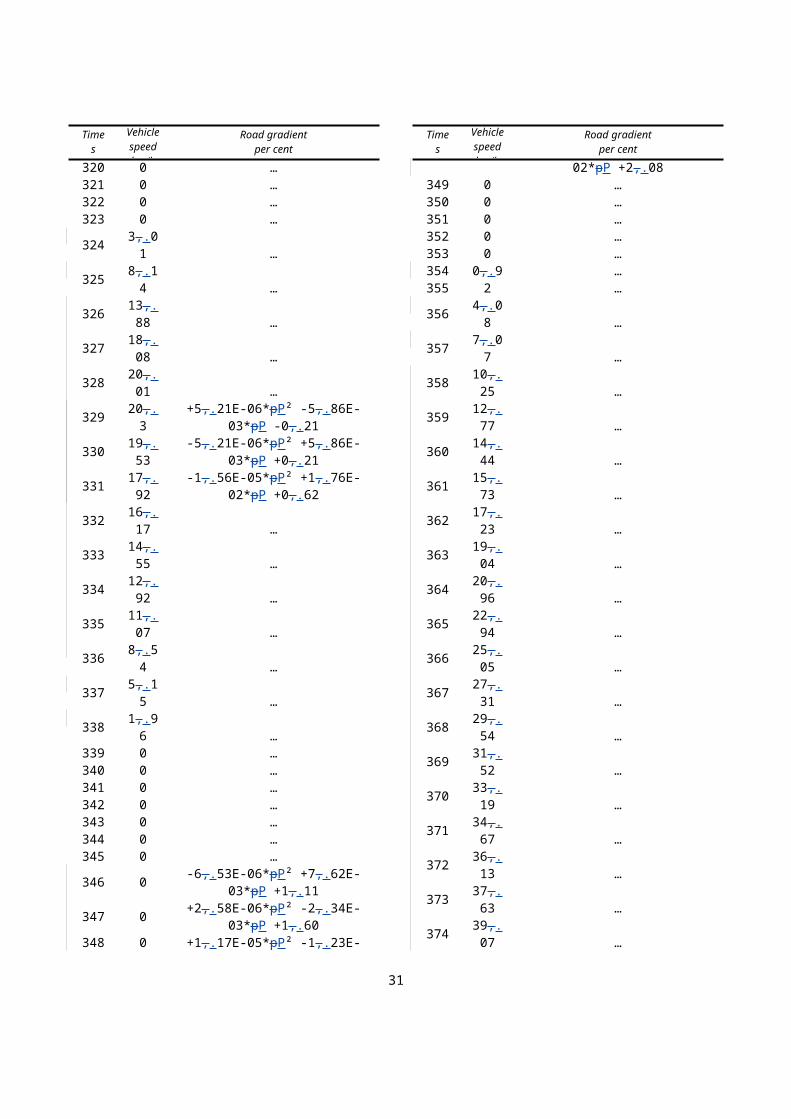
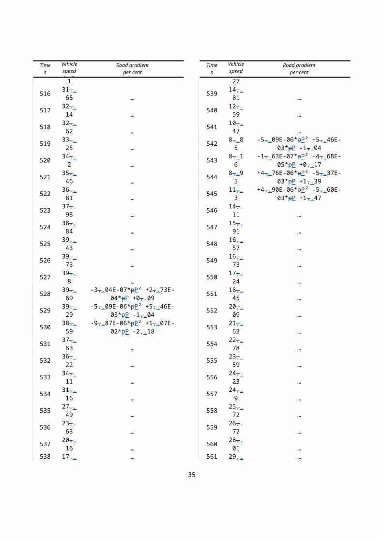
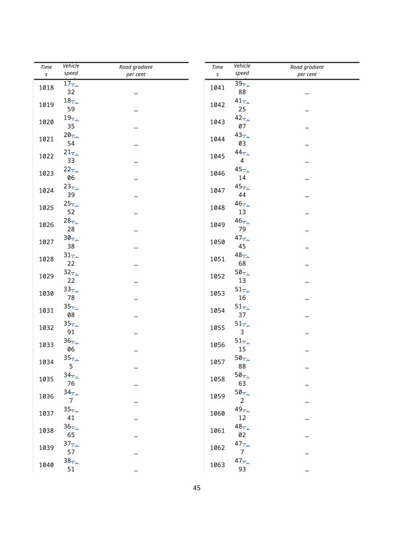
(b) WHVC vehicle schedule

P = rated power of hybrid system as specified in Annex 9 or Annex 10, respectively

Road gradient from the previous time step shall be used where a placeholder (…) is set.

Times

Vehicle speedkm/h

Road gradientper cent

1 0 +5.02E-06*pP² -6.80E-03*pP +0.772 0 …3 0 …4 0 …5 0 …6 0 …7 2,.35 …8 5,.57 …9 8,.18 …

10 9,.37 …11 9,.86 …12 10,.18 …13 10,.38 …14 10,.57 …15 10,.95 …16 11,.56 …17 12,.22 …18 12,.97 …19 14,.33 …20 16,.38 …21 18,.4 …22 19,.86 …23 20,.85 …24 21,.52 …25 21,.89 …26 21,.98 …27 21,.91 +1,.67E-06*pP² -2,.27E-03*pP +0,.2628 21,.68 -1,.67E-06*pP² +2,.27E-03*pP -0,.2629 21,.21 -5,.02E-06*pP² +6,.80E-03*pP -0,.7730 20,.44 …31 19,.24 …32 17,.57 …33 15,.53 …34 13,.77 …35 12,.95 …36 12,.95 …37 13,.35 …38 13,.75 …39 13,.82 …40 13,.41 …41 12,.26 …42 9,.82 …

Times

Vehicle speedkm/h


43 5,.96 …44 2,.2 …45 0 …46 0 …47 0 -1,.40E-06*pP² +2,.31E-03*pP -0,.8148 0 +2,.22E-06*pP² -2,.19E-03*pP -0,.8649 0 +5,.84E-06*pP² -6,.68E-03*pP -0,.9150 1,.87 …51 4,.97 …52 8,.4 …53 9,.9 …54 11,.42 …55 15,.11 …56 18,.46 …57 20,.21 …58 22,.13 …59 24,.17 …60 25,.56 …61 26,.97 …62 28,.83 …63 31,.05 …64 33,.72 …65 36 …66 37,.91 …67 39,.65 …68 41,.23 …69 42,.85 …70 44,.1 …71 44,.37 …72 44,.3 …73 44,.17 …74 44,.13 …75 44,.17 …76 44,.51 +3,.10E-06*pP² -3,.89E-03*pP -0,.7677 45,.16 +3,.54E-07*pP² -1,.10E-03*pP -0,.6178 45,.64 -2,.39E-06*pP² +1,.69E-03*pP -0,.4779 46,.16 …80 46,.99 …81 48,.19 …82 49,.32 …83 49,.7 …84 49,.5 …

19

Times

Vehicle speedkm/h


85 48,.98 …86 48,.65 …87 48,.65 …88 48,.87 …89 48,.97 …90 48,.96 …91 49,.15 …92 49,.51 …93 49,.74 …94 50,.31 …95 50,.78 …96 50,.75 …97 50,.78 …98 51,.21 …99 51,.6 …

100 51,.89 …101 52,.04 …102 51,.99 …103 51,.99 …104 52,.36 …105 52,.58 …106 52,.47 …107 52,.03 …108 51,.46 …109 51,.31 …110 51,.45 …111 51,.48 …112 51,.29 …113 51,.12 …114 50,.96 …115 50,.81 …116 50,.86 …117 51,.34 …118 51,.68 …119 51,.58 …120 51,.36 …121 51,.39 …122 50,.98 -1,.91E-06*pP² +1,.91E-03*pP -0,.06123 48,.63 -1,.43E-06*pP² +2,.13E-03*pP +0,.34124 44,.83 -9,.50E-07*pP² +2,.35E-03*pP +0,.74125 40,.3 …126 35,.65 …127 30,.23 …128 24,.08 …129 18,.96 …130 14,.19 …131 8,.72 …132 3,.41 …

Times

Vehicle speedkm/h


133 0,.64 …134 0 …135 0 …136 0 …137 0 …138 0 +2,.18E-06*pP² -1,.58E-03*pP +1,.27139 0 +5,.31E-06*pP² -5,.52E-03*pP +1,.80140 0 +8,.44E-06*pP² -9,.46E-03*pP +2,.33141 0 …142 0,.63 …143 1,.56 …144 2,.99 …145 4,.5 …146 5,.39 …147 5,.59 …148 5,.45 …149 5,.2 …150 4,.98 …151 4,.61 …152 3,.89 …153 3,.21 …154 2,.98 …155 3,.31 …156 4,.18 …157 5,.07 …158 5,.52 …159 5,.73 …160 6,.06 …161 6,.76 …162 7,.7 …163 8,.34 …164 8,.51 …165 8,.22 …166 7,.22 …167 5,.82 …168 4,.75 …169 4,.24 …170 4,.05 …171 3,.98 …172 3,.91 …173 3,.86 …174 4,.17 …175 5,.32 …176 7,.53 …177 10,.89 …178 14,.81 …179 17,.56 …180 18,.38 +2,.81E-06*pP² -3,.15E-03*pP +0,.78

20

Times

Vehicle speedkm/h


181 17,.49 -2,.81E-06*pP² +3,.15E-03*pP -0,.78182 15,.18 -8,.44E-06*pP² +9,.46E-03*pP -2,.33183 13,.08 …184 12,.23 …185 12,.03 …186 11,.72 …187 10,.69 …188 8,.68 …189 6,.2 …190 4,.07 …191 2,.65 …192 1,.92 …193 1,.69 …194 1,.68 …195 1,.66 …196 1,.53 …197 1,.3 …198 1 …199 0,.77 …200 0,.63 …201 0,.59 …202 0,.59 …203 0,.57 …204 0,.53 …205 0,.5 …206 0 …207 0 …208 0 …209 0 …210 0 …211 0 …212 0 …213 0 …214 0 …215 0 …216 0 …217 0 -5,.63E-06*pP² +6,.31E-03*pP -1,.56218 0 -2,.81E-06*pP² +3,.15E-03*pP -0,.78

219 0 +0,.00E+00*pP² +0,.00E+00*pP +0,.00

220 0 …221 0 …222 0 …223 0 …224 0 …225 0 …226 0,.73 …227 0,.73 …

Times

Vehicle speedkm/h


228 0 …229 0 …230 0 …231 0 …232 0 …233 0 …234 0 …235 0 …236 0 …237 0 …238 0 …239 0 …240 0 …241 0 …242 0 +6,.51E-06*pP² -6,.76E-03*pP +1,.50243 0 +1,.30E-05*pP² -1,.35E-02*pP +3,.00244 0 +1,.95E-05*pP² -2,.03E-02*pP +4,.49245 0 …246 0 …247 0 …248 0 …249 0 …250 0 …251 0 …252 0 …253 1,.51 …254 4,.12 …255 7,.02 …256 9,.45 …257 11,.86 …258 14,.52 …259 17,.01 …260 19,.48 …261 22,.38 …262 24,.75 …263 25,.55 +6,.51E-06*pP² -6,.76E-03*pP +1,.50264 25,.18 -6,.51E-06*pP² +6,.76E-03*pP -1,.50265 23,.94 -1,.95E-05*pP² +2,.03E-02*pP -4,.49266 22,.35 …267 21,.28 …268 20,.86 …269 20,.65 …270 20,.18 …271 19,.33 …272 18,.23 …273 16,.99 …274 15,.56 …275 13,.76 …

21

Times

Vehicle speedkm/h


276 11,.5 …277 8,.68 …278 5,.2 …279 1,.99 …280 0 …281 0 -1,.30E-05*pP² +1,.35E-02*pP -3,.00282 0 -6,.51E-06*pP² +6,.76E-03*pP -1,.50

283 0,.5 +0,.00E+00*pP² +0,.00E+00*pP +0,.00

284 0,.57 …285 0,.6 …286 0,.58 …287 0 …288 0 …289 0 …290 0 …291 0 …292 0 …293 0 …294 0 …295 0 …296 0 …297 0 …298 0 …299 0 …300 0 …301 0 …302 0 …303 0 …304 0 …305 0 +5,.21E-06*pP² -5,.86E-03*pP -0,.21306 0 +1,.04E-05*pP² -1,.17E-02*pP -0,.42307 0 +1,.56E-05*pP² -1,.76E-02*pP -0,.62308 0 …309 0 …310 0 …311 0 …312 0 …313 0 …314 0 …315 0 …316 0 …317 0 …318 0 …319 0 …320 0 …321 0 …322 0 …

Times

Vehicle speedkm/h


323 0 …324 3,.01 …325 8,.14 …326 13,.88 …327 18,.08 …328 20,.01 …329 20,.3 +5,.21E-06*pP² -5,.86E-03*pP -0,.21330 19,.53 -5,.21E-06*pP² +5,.86E-03*pP +0,.21331 17,.92 -1,.56E-05*pP² +1,.76E-02*pP +0,.62332 16,.17 …333 14,.55 …334 12,.92 …335 11,.07 …336 8,.54 …337 5,.15 …338 1,.96 …339 0 …340 0 …341 0 …342 0 …343 0 …344 0 …345 0 …346 0 -6,.53E-06*pP² +7,.62E-03*pP +1,.11347 0 +2,.58E-06*pP² -2,.34E-03*pP +1,.60348 0 +1,.17E-05*pP² -1,.23E-02*pP +2,.08349 0 …350 0 …351 0 …352 0 …353 0 …354 0,.9 …355 2 …356 4,.08 …357 7,.07 …358 10,.25 …359 12,.77 …360 14,.44 …361 15,.73 …362 17,.23 …363 19,.04 …364 20,.96 …365 22,.94 …366 25,.05 …367 27,.31 …368 29,.54 …369 31,.52 …370 33,.19 …

22

Times

Vehicle speedkm/h


371 34,.67 …372 36,.13 …373 37,.63 …374 39,.07 …375 40,.08 …376 40,.44 …377 40,.26 +6,.91E-06*pP² -7,.10E-03*pP +0,.94378 39,.29 +2,.13E-06*pP² -1,.91E-03*pP -0,.20379 37,.23 -2,.65E-06*pP² +3,.28E-03*pP -1,.33380 34,.14 …381 30,.18 …382 25,.71 …383 21,.58 …384 18,.5 …385 16,.56 …386 15,.39 …387 14,.77 +2,.55E-06*pP² -2,.25E-03*pP +0,.26388 14,.58 +7,.75E-06*pP² -7,.79E-03*pP +1,.86389 14,.72 +1,.30E-05*pP² -1,.33E-02*pP +3,.46390 15,.44 …391 16,.92 …392 18,.69 …393 20,.26 …394 21,.63 …395 22,.91 …396 24,.13 …397 25,.18 …398 26,.16 …399 27,.41 …400 29,.18 …401 31,.36 …402 33,.51 …403 35,.33 …404 36,.94 …405 38,.6 …406 40,.44 …407 42,.29 …408 43,.73 …409 44,.47 …410 44,.62 …411 44,.41 +8,.17E-06*pP² -8,.13E-03*pP +2,.32412 43,.96 +3,.39E-06*pP² -2,.94E-03*pP +1,.18413 43,.41 -1,.39E-06*pP² +2,.25E-03*pP +0,.04414 42,.83 …415 42,.15 …416 41,.28 …417 40,.17 …418 38,.9 …

Times

Vehicle speedkm/h


419 37,.59 …420 36,.39 …421 35,.33 …422 34,.3 …423 33,.07 …424 31,.41 …425 29,.18 …426 26,.41 …427 23,.4 …428 20,.9 …429 19,.59 +8,.47E-07*pP² -6,.08E-04*pP +0,.36430 19,.36 +3,.09E-06*pP² -3,.47E-03*pP +0,.69431 19,.79 +5,.33E-06*pP² -6,.33E-03*pP +1,.01432 20,.43 …433 20,.71 …434 20,.56 …435 19,.96 …436 20,.22 …437 21,.48 …438 23,.67 …439 26,.09 …440 28,.16 …441 29,.75 …442 30,.97 …443 31,.99 …444 32,.84 …445 33,.33 …446 33,.45 …447 33,.27 +5,.50E-07*pP² -1,.13E-03*pP -0,.13448 32,.66 -4,.23E-06*pP² +4,.06E-03*pP -1,.26449 31,.73 -9,.01E-06*pP² +9,.25E-03*pP -2,.40450 30,.58 …451 29,.2 …452 27,.56 …453 25,.71 …454 23,.76 …455 21,.87 …456 20,.15 …457 18,.38 …458 15,.93 …459 12,.33 …460 7,.99 …461 4,.19 …462 1,.77 …463 0,.69 -1,.66E-06*pP² +1,.67E-03*pP -0,.86464 1,.13 +5,.69E-06*pP² -5,.91E-03*pP +0,.68465 2,.2 +1,.30E-05*pP² -1,.35E-02*pP +2,.23466 3,.59 …

23

Times

Vehicle speedkm/h


467 4,.88 …468 5,.85 …469 6,.72 …470 8,.02 …471 10,.02 …472 12,.59 …473 15,.43 …474 18,.32 …475 21,.19 …476 24 …477 26,.75 …478 29,.53 …479 32,.31 …480 34,.8 …481 36,.73 …482 38,.08 …483 39,.11 …484 40,.16 …485 41,.18 …486 41,.75 …487 41,.87 +8,.26E-06*pP² -8,.29E-03*pP +1,.09488 41,.43 +3,.47E-06*pP² -3,.10E-03*pP -0,.05489 39,.99 -1,.31E-06*pP² +2,.09E-03*pP -1,.19490 37,.71 …491 34,.93 …492 31,.79 …493 28,.65 …494 25,.92 …495 23,.91 …496 22,.81 +6,.20E-07*pP² -2,.47E-04*pP -0,.38497 22,.53 +2,.55E-06*pP² -2,.58E-03*pP +0,.43498 22,.62 +4,.48E-06*pP² -4,.92E-03*pP +1,.23499 22,.95 …500 23,.51 …501 24,.04 …502 24,.45 …503 24,.81 …504 25,.29 …505 25,.99 …506 26,.83 …507 27,.6 …508 28,.17 …509 28,.63 …510 29,.04 …511 29,.43 …512 29,.78 …513 30,.13 …514 30,.57 …

Times

Vehicle speedkm/h


515 31,.1 …516 31,.65 …517 32,.14 …518 32,.62 …519 33,.25 …520 34,.2 …521 35,.46 …522 36,.81 …523 37,.98 …524 38,.84 …525 39,.43 …526 39,.73 …527 39,.8 …528 39,.69 -3,.04E-07*pP² +2,.73E-04*pP +0,.09529 39,.29 -5,.09E-06*pP² +5,.46E-03*pP -1,.04530 38,.59 -9,.87E-06*pP² +1,.07E-02*pP -2,.18531 37,.63 …532 36,.22 …533 34,.11 …534 31,.16 …535 27,.49 …536 23,.63 …537 20,.16 …538 17,.27 …539 14,.81 …540 12,.59 …541 10,.47 …542 8,.85 -5,.09E-06*pP² +5,.46E-03*pP -1,.04543 8,.16 -1,.63E-07*pP² +4,.68E-05*pP +0,.17544 8,.95 +4,.76E-06*pP² -5,.37E-03*pP +1,.39545 11,.3 +4,.90E-06*pP² -5,.60E-03*pP +1,.47546 14,.11 …547 15,.91 …548 16,.57 …549 16,.73 …550 17,.24 …551 18,.45 …552 20,.09 …553 21,.63 …554 22,.78 …555 23,.59 …556 24,.23 …557 24,.9 …558 25,.72 …559 26,.77 …560 28,.01 …561 29,.23 …562 30,.06 …

24

Times

Vehicle speedkm/h


563 30,.31 …564 30,.29 +1,.21E-07*pP² -4,.06E-04*pP +0,.33565 30,.05 -4,.66E-06*pP² +4,.79E-03*pP -0,.81566 29,.44 -9,.44E-06*pP² +9,.98E-03*pP -1,.95567 28,.6 …568 27,.63 …569 26,.66 …570 26,.03 -4,.66E-06*pP² +4,.79E-03*pP -0,.81571 25,.85 +1,.21E-07*pP² -4,.06E-04*pP +0,.33572 26,.14 +4,.90E-06*pP² -5,.60E-03*pP +1,.47573 27,.08 …574 28,.42 …575 29,.61 …576 30,.46 …577 30,.99 …578 31,.33 …579 31,.65 …580 32,.02 …581 32,.39 …582 32,.68 …583 32,.84 …584 32,.93 …585 33,.22 …586 33,.89 …587 34,.96 …588 36,.28 …589 37,.58 …590 38,.58 …591 39,.1 …592 39,.22 …593 39,.11 …594 38,.8 …595 38,.31 …596 37,.73 …597 37,.24 …598 37,.06 …599 37,.1 …600 37,.42 …601 38,.17 …602 39,.19 …603 40,.31 …604 41,.46 …605 42,.44 …606 42,.95 …607 42,.9 …608 42,.43 …609 41,.74 …610 41,.04 …

Times

Vehicle speedkm/h


611 40,.49 …612 40,.8 …613 41,.66 …614 42,.48 …615 42,.78 +1,.21E-07*pP² -4,.06E-04*pP +0,.33616 42,.39 -4,.66E-06*pP² +4,.79E-03*pP -0,.81617 40,.78 -9,.44E-06*pP² +9,.98E-03*pP -1,.95618 37,.72 …619 33,.29 …620 27,.66 …621 21,.43 …622 15,.62 …623 11,.51 …624 9,.69 -4,.66E-06*pP² +4,.79E-03*pP -0,.81625 9,.46 +1,.21E-07*pP² -4,.06E-04*pP +0,.33626 10,.21 +4,.90E-06*pP² -5,.60E-03*pP +1,.47627 11,.78 …628 13,.6 …629 15,.33 …630 17,.12 …631 18,.98 …632 20,.73 …633 22,.17 …634 23,.29 …635 24,.19 …636 24,.97 …637 25,.6 …638 25,.96 …639 25,.86 +1,.21E-07*pP² -4,.06E-04*pP +0,.33640 24,.69 -4,.66E-06*pP² +4,.79E-03*pP -0,.81641 21,.85 -9,.44E-06*pP² +9,.98E-03*pP -1,.95642 17,.45 …643 12,.34 …644 7,.59 …645 4 …646 1,.76 …647 0 …648 0 …649 0 …650 0 …651 0 …652 0 -3,.90E-06*pP² +4,.11E-03*pP -1,.07653 0 +1,.64E-06*pP² -1,.77E-03*pP -0,.19654 0 +7,.18E-06*pP² -7,.64E-03*pP +0,.70655 0 …656 0 …657 0 …658 2,.96 …

25

Times

Vehicle speedkm/h


659 7,.9 …660 13,.49 …661 18,.36 …662 22,.59 …663 26,.26 …664 29,.4 …665 32,.23 …666 34,.91 …667 37,.39 …668 39,.61 …669 41,.61 …670 43,.51 …671 45,.36 …672 47,.17 …673 48,.95 …674 50,.73 …675 52,.36 …676 53,.74 …677 55,.02 …678 56,.24 …679 57,.29 …680 58,.18 …681 58,.95 …682 59,.49 …683 59,.86 …684 60,.3 …685 61,.01 …686 61,.96 …687 63,.05 …688 64,.16 …689 65,.14 …690 65,.85 …691 66,.22 …692 66,.12 +2,.39E-06*pP² -2,.55E-03*pP +0,.23693 65,.01 -2,.39E-06*pP² +2,.55E-03*pP -0,.23694 62,.22 -7,.18E-06*pP² +7,.64E-03*pP -0,.70695 57,.44 …696 51,.47 …697 45,.98 …698 41,.72 …699 38,.22 …700 34,.65 …701 30,.65 …702 26,.46 …703 22,.32 …704 18,.15 …705 13,.79 …706 9,.29 …

Times

Vehicle speedkm/h


707 4,.98 …708 1,.71 …709 0 …710 0 …711 0 …712 0 …713 0 …714 0 …715 0 …716 0 …717 0 …718 0 …719 0 …720 0 …721 0 …722 0 …723 0 …724 0 …725 0 …726 0 …727 0 …728 0 …729 0 …730 0 …731 0 …732 0 …733 0 …734 0 …735 0 …736 0 …737 0 …738 0 …739 0 -2,.53E-06*pP² +2,.43E-03*pP +0,.05740 0 +2,.12E-06*pP² -2,.78E-03*pP +0,.81741 0 +6,.77E-06*pP² -7,.99E-03*pP +1,.56742 0 …743 0 …744 0 …745 0 …746 0 …747 0 …748 0 …749 0 …750 0 …751 0 …752 0 …753 0 …754 0 …

26

Times

Vehicle speedkm/h


755 0 …756 0 …757 0 …758 0 …759 0 …760 0 …761 0 …762 0 …763 0 …764 0 …765 0 …766 0 …767 0 …768 0 …769 0 …770 0 …771 0 …772 1,.6 …773 5,.03 …774 9,.49 …775 13 …776 14,.65 …777 15,.15 …778 15,.67 …779 16,.76 …780 17,.88 …781 18,.33 …782 18,.31 +2,.26E-06*pP² -2,.66E-03*pP +0,.52783 18,.05 -2,.26E-06*pP² +2,.66E-03*pP -0,.52784 17,.39 -6,.77E-06*pP² +7,.99E-03*pP -1,.56785 16,.35 …786 14,.71 …787 11,.71 …788 7,.81 …789 5,.25 -2,.26E-06*pP² +2,.66E-03*pP -0,.52790 4,.62 +2,.26E-06*pP² -2,.66E-03*pP +0,.52791 5,.62 +6,.77E-06*pP² -7,.99E-03*pP +1,.56792 8,.24 …793 10,.98 …794 13,.15 …795 15,.47 …796 18,.19 …797 20,.79 …798 22,.5 …799 23,.19 …800 23,.54 …801 24,.2 …802 25,.17 …

Times

Vehicle speedkm/h


803 26,.28 …804 27,.69 …805 29,.72 …806 32,.17 …807 34,.22 …808 35,.31 …809 35,.74 …810 36,.23 …811 37,.34 …812 39,.05 …813 40,.76 …814 41,.82 …815 42,.12 …816 42,.08 …817 42,.27 …818 43,.03 …819 44,.14 …820 45,.13 …821 45,.84 …822 46,.4 …823 46,.89 …824 47,.34 …825 47,.66 …826 47,.77 …827 47,.78 …828 47,.64 +2,.26E-06*pP² -2,.66E-03*pP +0,.52829 47,.23 -2,.26E-06*pP² +2,.66E-03*pP -0,.52830 46,.66 -6,.77E-06*pP² +7,.99E-03*pP -1,.56831 46,.08 …832 45,.45 …833 44,.69 …834 43,.73 …835 42,.55 …836 41,.14 …837 39,.56 …838 37,.93 …839 36,.69 …840 36,.27 …841 36,.42 …842 37,.14 …843 38,.13 …844 38,.55 …845 38,.42 …846 37,.89 …847 36,.89 …848 35,.53 …849 34,.01 …850 32,.88 -2,.26E-06*pP² +2,.66E-03*pP -0,.52

27

Times

Vehicle speedkm/h


851 32,.52 +2,.26E-06*pP² -2,.66E-03*pP +0,.52852 32,.7 +6,.77E-06*pP² -7,.99E-03*pP +1,.56853 33,.48 …854 34,.97 …855 36,.78 …856 38,.64 …857 40,.48 …858 42,.34 …859 44,.16 …860 45,.9 …861 47,.55 …862 49,.09 …863 50,.42 …864 51,.49 …865 52,.23 …866 52,.58 …867 52,.63 …868 52,.49 +2,.26E-06*pP² -2,.66E-03*pP +0,.52869 52,.19 -2,.26E-06*pP² +2,.66E-03*pP -0,.52870 51,.82 -6,.77E-06*pP² +7,.99E-03*pP -1,.56871 51,.43 …872 51,.02 …873 50,.61 …874 50,.26 …875 50,.06 …876 49,.97 …877 49,.67 …878 48,.86 …879 47,.53 …880 45,.82 …881 43,.66 …882 40,.91 …883 37,.78 …884 34,.89 …885 32,.69 …886 30,.99 …887 29,.31 …888 27,.29 …889 24,.79 …890 21,.78 …891 18,.51 …892 15,.1 …893 11,.06 …894 6,.28 …895 2,.24 …896 0 …897 0 …898 0 …

Times

Vehicle speedkm/h


899 0 -3,.61E-06*pP² +4,.12E-03*pP -0,.93900 0 -4,.47E-07*pP² +2,.44E-04*pP -0,.31901 0 +2,.71E-06*pP² -3,.63E-03*pP +0,.32902 2,.56 …903 4,.81 …904 6,.38 …905 8,.62 …906 10,.37 …907 11,.17 …908 13,.32 …909 15,.94 …910 16,.89 …911 17,.13 …912 18,.04 …913 19,.96 …914 22,.05 …915 23,.65 …916 25,.72 …917 28,.62 …918 31,.99 …919 35,.07 …920 37,.42 …921 39,.65 …922 41,.78 …923 43,.04 …924 43,.55 …925 42,.97 …926 41,.08 …927 40,.38 …928 40,.43 …929 40,.4 …930 40,.25 …931 40,.32 …932 40,.8 …933 41,.71 …934 43,.16 …935 44,.84 …936 46,.42 …937 47,.91 …938 49,.08 …939 49,.66 …940 50,.15 …941 50,.94 …942 51,.69 …943 53,.5 …944 55,.9 …945 57,.11 …946 57,.88 …

28

Times

Vehicle speedkm/h


947 58,.63 …948 58,.75 …949 58,.26 …950 58,.03 …951 58,.28 …952 58,.67 …953 58,.76 …954 58,.82 …955 59,.09 …956 59,.38 …957 59,.72 …958 60,.04 …959 60,.13 +2,.08E-06*pP² -2,.00E-03*pP +0,.46960 59,.33 +1,.44E-06*pP² -3,.72E-04*pP +0,.61961 58,.52 +8,.03E-07*pP² +1,.26E-03*pP +0,.75962 57,.82 …963 56,.68 …964 55,.36 …965 54,.63 …966 54,.04 …967 53,.15 …968 52,.02 +1,.44E-06*pP² -3,.72E-04*pP +0,.61969 51,.37 +2,.08E-06*pP² -2,.00E-03*pP +0,.46970 51,.41 +2,.71E-06*pP² -3,.63E-03*pP +0,.32971 52,.2 …972 53,.52 …973 54,.34 …974 54,.59 …975 54,.92 …976 55,.69 …977 56,.51 …978 56,.73 +2,.08E-06*pP² -2,.00E-03*pP +0,.46979 56,.33 +1,.44E-06*pP² -3,.72E-04*pP +0,.61980 55,.38 +8,.03E-07*pP² +1,.26E-03*pP +0,.75981 54,.99 …982 54,.75 …983 54,.11 …984 53,.32 …985 52,.41 …986 51,.45 …987 50,.86 …988 50,.48 …989 49,.6 …990 48,.55 …991 47,.87 …992 47,.42 …993 46,.86 …994 46,.08 …

Times

Vehicle speedkm/h


995 45,.07 …996 43,.58 …997 41,.04 …998 38,.39 …999 35,.69 …

1000 32,.68 …1001 29,.82 …1002 26,.97 …1003 24,.03 …1004 21,.67 …1005 20,.34 …1006 18,.9 …1007 16,.21 …1008 13,.84 …1009 12,.25 …1010 10,.4 …1011 7,.94 …1012 6,.05 +1,.48E-07*pP² +2,.76E-04*pP +0,.251013 5,.67 -5,.06E-07*pP² -7,.04E-04*pP -0,.261014 6,.03 -1,.16E-06*pP² -1,.68E-03*pP -0,.771015 7,.68 …1016 10,.97 …1017 14,.72 …1018 17,.32 …1019 18,.59 …1020 19,.35 …1021 20,.54 …1022 21,.33 …1023 22,.06 …1024 23,.39 …1025 25,.52 …1026 28,.28 …1027 30,.38 …1028 31,.22 …1029 32,.22 …1030 33,.78 …1031 35,.08 …1032 35,.91 …1033 36,.06 …1034 35,.5 …1035 34,.76 …1036 34,.7 …1037 35,.41 …1038 36,.65 …1039 37,.57 …1040 38,.51 …1041 39,.88 …1042 41,.25 …

29

Times

Vehicle speedkm/h


1043 42,.07 …1044 43,.03 …1045 44,.4 …1046 45,.14 …1047 45,.44 …1048 46,.13 …1049 46,.79 …1050 47,.45 …1051 48,.68 …1052 50,.13 …1053 51,.16 …1054 51,.37 …1055 51,.3 …1056 51,.15 …1057 50,.88 …1058 50,.63 …1059 50,.2 …1060 49,.12 …1061 48,.02 …1062 47,.7 …1063 47,.93 …1064 48,.57 …1065 48,.88 …1066 49,.03 …1067 48,.94 …1068 48,.32 …1069 47,.97 …1070 47,.92 -1,.80E-06*pP² -5,.59E-05*pP -0,.621071 47,.54 -2,.43E-06*pP² +1,.57E-03*pP -0,.481072 46,.79 -3,.07E-06*pP² +3,.20E-03*pP -0,.341073 46,.13 …1074 45,.73 …1075 45,.17 …1076 44,.43 …1077 43,.59 …1078 42,.68 …1079 41,.89 …1080 41,.09 …1081 40,.38 …1082 39,.99 …1083 39,.84 …1084 39,.46 …1085 39,.15 …1086 38,.9 …1087 38,.67 …1088 39,.03 …1089 40,.37 …1090 41,.03 …

Times

Vehicle speedkm/h


1091 40,.76 …1092 40,.02 …1093 39,.6 …1094 39,.37 …1095 38,.84 …1096 37,.93 …1097 37,.19 …1098 36,.21 -2,.43E-06*pP² +1,.57E-03*pP -0,.481099 35,.32 -1,.80E-06*pP² -5,.59E-05*pP -0,.621100 35,.56 -1,.16E-06*pP² -1,.68E-03*pP -0,.771101 36,.96 …1102 38,.12 …1103 38,.71 …1104 39,.26 …1105 40,.64 …1106 43,.09 …1107 44,.83 …1108 45,.33 …1109 45,.24 …1110 45,.14 …1111 45,.06 …1112 44,.82 …1113 44,.53 …1114 44,.77 …1115 45,.6 …1116 46,.28 …1117 47,.18 …1118 48,.49 …1119 49,.42 …1120 49,.56 …1121 49,.47 …1122 49,.28 …1123 48,.58 …1124 48,.03 …1125 48,.2 …1126 48,.72 …1127 48,.91 …1128 48,.93 …1129 49,.05 …1130 49,.23 …1131 49,.28 -1,.80E-06*pP² -5,.59E-05*pP -0,.621132 48,.84 -2,.43E-06*pP² +1,.57E-03*pP -0,.481133 48,.12 -3,.07E-06*pP² +3,.20E-03*pP -0,.341134 47,.8 …1135 47,.42 …1136 45,.98 …1137 42,.96 …1138 39,.38 …

30

Times

Vehicle speedkm/h


1139 35,.82 …1140 31,.85 …1141 26,.87 …1142 21,.41 …1143 16,.41 …1144 12,.56 …1145 10,.41 …1146 9,.07 …1147 7,.69 …1148 6,.28 …1149 5,.08 …1150 4,.32 …1151 3,.32 …1152 1,.92 …1153 1,.07 …1154 0,.66 …1155 0 …1156 0 …1157 0 …1158 0 …1159 0 …1160 0 …1161 0 …1162 0 …1163 0 …1164 0 …1165 0 …1166 0 …1167 0 …1168 0 …1169 0 …1170 0 …1171 0 …1172 0 …1173 0 …1174 0 …1175 0 -7,.73E-07*pP² +5,.68E-04*pP +0,.071176 0 +1,.53E-06*pP² -2,.06E-03*pP +0,.471177 0 +3,.82E-06*pP² -4,.70E-03*pP +0,.871178 0 …1179 0 …1180 0 …1181 0 …1182 0 …1183 0 …1184 0 …1185 0 …1186 0 …

Times

Vehicle speedkm/h


1187 0 …1188 0 …1189 0 …1190 0 …1191 0 …1192 0 …1193 0 …1194 0 …1195 0 …1196 1,.54 …1197 4,.85 …1198 9,.06 …1199 11,.8 …1200 12,.42 …1201 12,.07 …1202 11,.64 …1203 11,.69 …1204 12,.91 …1205 15,.58 …1206 18,.69 …1207 21,.04 …1208 22,.62 …1209 24,.34 …1210 26,.74 …1211 29,.62 …1212 32,.65 …1213 35,.57 …1214 38,.07 …1215 39,.71 …1216 40,.36 …1217 40,.6 …1218 41,.15 …1219 42,.23 …1220 43,.61 …1221 45,.08 …1222 46,.58 …1223 48,.13 …1224 49,.7 …1225 51,.27 …1226 52,.8 …1227 54,.3 …1228 55,.8 …1229 57,.29 …1230 58,.73 …1231 60,.12 …1232 61,.5 …1233 62,.94 …1234 64,.39 …

31

Times

Vehicle speedkm/h


1235 65,.52 …1236 66,.07 …1237 66,.19 …1238 66,.19 …1239 66,.43 …1240 67,.07 …1241 68,.04 …1242 69,.12 …1243 70,.08 …1244 70,.91 …1245 71,.73 …1246 72,.66 …1247 73,.67 …1248 74,.55 …1249 75,.18 …1250 75,.59 …1251 75,.82 …1252 75,.9 …1253 75,.92 …1254 75,.87 …1255 75,.68 …1256 75,.37 …1257 75,.01 +7,.07E-06*pP² -7,.30E-03*pP +1,.191258 74,.55 +1,.03E-05*pP² -9,.91E-03*pP +1,.511259 73,.8 +1,.36E-05*pP² -1,.25E-02*pP +1,.831260 72,.71 …1261 71,.39 …1262 70,.02 …1263 68,.71 …1264 67,.52 …1265 66,.44 …1266 65,.45 …1267 64,.49 …1268 63,.54 …1269 62,.6 …1270 61,.67 …1271 60,.69 …1272 59,.64 …1273 58,.6 …1274 57,.64 …1275 56,.79 …1276 55,.95 …1277 55,.09 …1278 54,.2 …1279 53,.33 …1280 52,.52 …1281 51,.75 …1282 50,.92 …

Times

Vehicle speedkm/h


1283 49,.9 …1284 48,.68 …1285 47,.41 …

1286 46,.5+9,40E-06*p² -8,92E-03*p

+1,50+1.06E-05*P² -1.01E-02*P +1.57

1287 46,.22 +5,22E7.62E-06*p² -5,32EP² -7.70E-03*pP +1,16.30

1288 46,.44 +1,04E4.65E-06*p² -1,72EP² -5.29E-03*p +0,82P +1.03

1289 47,.35 …1290 49,.01 …1291 50,.93 …1292 52,.79 …1293 54,.66 …1294 56,.6 …1295 58,.55 …1296 60,.47 …1297 62,.28 …1298 63,.9 …1299 65,.2 …1300 66,.02 …1301 66,.39 …1302 66,.74 …1303 67,.43 …1304 68,.44 …1305 69,.52 …1306 70,.53 …1307 71,.47 …1308 72,.32 …1309 72,.89 …1310 73,.07 …1311 73,.03 …+2.39E-06*P² -3.13E-03*P +0.891312 72,.94 …+1.26E-07*P² -9.74E-04*P +0.741313 73,.01 …-2.14E-06*P² +1.18E-03*P +0.601314 73,.44 …1315 74,.19 …1316 74,.81 …1317 75,.01 …1318 74,.99 …1319 74,.79 …1320 74,.41 …1321 74,.07 …1322 73,.77 …1323 73,.38 …1324 72,.79 …1325 71,.95 …1326 71,.06 …1327 70,.45 …

32

Times

Vehicle speedkm/h


1328 70,.23 …1329 70,.24 …1330 70,.32 …1331 70,.3 …1332 70,.05 …1333 69,.66 …

1334 69,.26 +4,29E1.12E-06*p² -4,33EP² -1.42E-03*p +1,14P +0.92

1335 68,.73 +7,54E4.37E-06*p² -6,94EP² -4.03E-03*pP +1,46.24

1336 67,.88 +1,08E-05*p² -9,54E+7.62E-06*P² -6.64E-03*pP +1,78.56

1337 66,.68 …1338 65,.29 …1339 63,.95 …

1340 62,.84 +7,54E4.37E-06*p² -6,94EP² -4.03E-03*pP +1,46.24

1341 62,.21 +4,29E1.12E-06*p² -4,33EP² -1.42E-03*p +1,14P +0.92

1342 62,.04 +1,04E-2.14E-06*p² -P² +1,72E.18E-03*pP +0,82.60

1343 62,.26 …1344 62,.87 …1345 63,.55 …1346 64,.12 …1347 64,.73 …1348 65,.45 …1349 66,.18 …1350 66,.97 …1351 67,.85 …1352 68,.74 …1353 69,.45 …1354 69,.92 …1355 70,.24 …1356 70,.49 …1357 70,.63 …1358 70,.68 …1359 70,.65 …

1360 70,.49 +4,29E1.12E-06*p² -4,33EP² -1.42E-03*p +1,14P +0.92

1361 70,.09 +7,54E4.37E-06*p² -6,94EP² -4.03E-03*pP +1,46.24

1362 69,.35 +1,08E-05*p² -9,54E+7.62E-06*P² -6.64E-03*pP +1,78.56

1363 68,.27 …1364 67,.09 …1365 65,.96 …1366 64,.87 …1367 63,.79 …1368 62,.82 +7,54E4.37E-06*p² -6,94EP² -4.03E-

Times

Vehicle speedkm/h


03*pP +1,46.24

1369 63,.03 +4,29E1.12E-06*p² -4,33EP² -1.42E-03*p +1,14P +0.92

1370 63,.62 +1,04E-2.14E-06*p² -P² +1,72E.18E-03*pP +0,82.60

1371 64,.8 …1372 65,.5 …

1373 65,.33 +4,29E1.12E-06*p² -4,33EP² -1.42E-03*p +1,14P +0.92

1374 63,.83 +7,54E4.37E-06*p² -6,94EP² -4.03E-03*pP +1,46.24

1375 62,.44 +1,08E-05*p² -9,54E+7.62E-06*P² -6.64E-03*pP +1,78.56

1376 61,.2 …1377 59,.58 …1378 57,.68 …1379 56,.4 …1380 54,.82 …

1381 52,.77 +8,89E6.78E-06*p² -8,29EP² -6.35E-03*pP +2,21.06

1382 52,.22 +6,99E5.95E-06*p² -7,03EP² -6.07E-03*pP +2,63.56

1383 52,.48 +5,09E.11E-06*pP² -5,77E.78E-03*pP +3,.06

1384 52,.74 …1385 53,.14 …1386 53,.03 …1387 52,.55 …1388 52,.19 …1389 51,.09 …1390 49,.88 …1391 49,.37 …1392 49,.26 …1393 49,.37 …1394 49,.88 …1395 50,.25 …1396 50,.17 …1397 50,.5 …1398 50,.83 …1399 51,.23 …1400 51,.67 …1401 51,.53 …1402 50,.17 …1403 49,.99 …1404 50,.32 …1405 51,.05 …1406 51,.45 …1407 52 …1408 52,.3 …1409 52,.22 …

33

Times

Vehicle speedkm/h


1410 52,.66 …1411 53,.18 …1412 53,.8 …1413 54,.53 …1414 55,.37 …1415 56,.29 …1416 57,.31 …1417 57,.94 …1418 57,.86 …1419 57,.75 …1420 58,.67 …1421 59,.4 …1422 59,.69 …1423 60,.02 …1424 60,.21 …1425 60,.83 …1426 61,.16 …1427 61,.6 …1428 62,.15 …

1429 62,.7 +2,29E.30E-06*pP² -3,17E.18E-03*pP +1,.81

1430 63,.65 -5,13E.04E-07*pP² -5,70E.74E-04*pP +0,.57

1431 64,.27 -3,.31E-06*pP² +2,.03E-03*pP -0,.681432 64,.31 …1433 64,.13 …1434 64,.27 …1435 65,.22 …1436 66,.25 …1437 67,.09 …1438 68,.37 …1439 69,.36 …1440 70,.57 …1441 71,.89 …1442 73,.35 …1443 74,.64 …1444 75,.81 …1445 77,.24 …1446 78,.63 …1447 79,.32 …1448 80,.2 …1449 81,.67 …1450 82,.11 …1451 82,.91 …1452 83,.43 …1453 83,.79 …1454 83,.5 …1455 84,.01 …1456 83,.43 …

Times

Vehicle speedkm/h


1457 82,.99 …1458 82,.77 …1459 82,.33 …1460 81,.78 …1461 81,.81 …1462 81,.05 …1463 80,.72 -6,.93E-06*pP² +5,.24E-03*pP -1,.211464 80,.61 -1,.05E-05*pP² +8,.45E-03*pP -1,.741465 80,.46 -1,.42E-05*pP² +1,.17E-02*pP -2,.271466 80,.42 …1467 80,.42 …1468 80,.24 …1469 80,.13 …1470 80,.39 …1471 80,.72 …1472 81,.01 …1473 81,.52 …1474 82,.4 …1475 83,.21 …1476 84,.05 …1477 84,.85 …1478 85,.42 …1479 86,.18 …1480 86,.45 …1481 86,.64 …1482 86,.57 …1483 86,.43 …1484 86,.58 …1485 86,.8 …1486 86,.65 …1487 86,.14 …1488 86,.36 …1489 86,.32 …1490 86,.25 …1491 85,.92 …1492 86,.14 …1493 86,.36 …1494 86,.25 …1495 86,.5 …1496 86,.14 …1497 86,.29 …1498 86,.4 …1499 86,.36 …1500 85,.63 …1501 86,.03 …1502 85,.92 …1503 86,.14 …1504 86,.32 …

34

Times

Vehicle speedkm/h


1505 85,.92 …1506 86,.11 …1507 85,.91 …1508 85,.83 …1509 85,.86 -1,.09E-05*pP² +9,.06E-03*pP -1,.951510 85,.5 -7,.66E-06*pP² +6,.45E-03*pP -1,.631511 84,.97 -4,.41E-06*pP² +3,.84E-03*pP -1,.311512 84,.8 …1513 84,.2 …1514 83,.26 …1515 82,.77 …1516 81,.78 …1517 81,.16 …1518 80,.42 …1519 79,.21 …1520 78,.83 …1521 78,.52 -5,.24E-06*pP² +4,.57E-03*pP -1,.181522 78,.52 -6,.08E-06*pP² +5,.30E-03*pP -1,.061523 78,.81 -6,.91E-06*pP² +6,.04E-03*pP -0,.931524 79,.26 …1525 79,.61 …1526 80,.15 …1527 80,.39 …1528 80,.72 …1529 81,.01 …1530 81,.52 …1531 82,.4 …1532 83,.21 …1533 84,.05 …1534 85,.15 …1535 85,.92 …1536 86,.98 …1537 87,.45 …1538 87,.54 …1539 87,.25 …1540 87,.04 …1541 86,.98 …1542 87,.05 …1543 87,.1 …1544 87,.25 …1545 87,.25 …1546 87,.07 …1547 87,.29 …1548 87,.14 …1549 87,.03 …1550 87,.25 …1551 87,.03 …1552 87,.03 …

Times

Vehicle speedkm/h


1553 87,.07 …1554 86,.81 …1555 86,.92 …1556 86,.66 …1557 86,.92 …1558 86,.59 …1559 86,.92 …1560 86,.59 …1561 86,.88 …1562 86,.7 …1563 86,.81 …1564 86,.81 …1565 86,.81 …1566 86,.81 …1567 86,.99 …1568 87,.03 …1569 86,.92 …1570 87,.1 …1571 86,.85 …1572 87,.14 …1573 86,.96 …1574 86,.85 …1575 86,.77 …1576 86,.81 …1577 86,.85 …1578 86,.74 …1579 86,.81 …1580 86,.7 …1581 86,.52 …1582 86,.7 …1583 86,.74 …1584 86,.81 …1585 86,.85 …1586 86,.92 …1587 86,.88 …1588 86,.85 …1589 87,.1 …1590 86,.81 …1591 86,.99 …1592 86,.81 …1593 87,.14 …1594 86,.81 …1595 86,.85 …1596 87,.03 …1597 86,.92 …1598 87,.14 …1599 86,.92 …1600 87,.03 …

35

Times

Vehicle speedkm/h


1601 86,.99 …1602 86,.96 …1603 87,.03 …1604 86,.85 …1605 87,.1 …1606 86,.81 …1607 87,.03 …1608 86,.77 …1609 86,.99 …1610 86,.96 …1611 86,.96 …1612 87,.07 …1613 86,.96 …1614 86,.92 …1615 87,.07 …1616 86,.92 …1617 87,.14 …1618 86,.96 …1619 87,.03 …1620 86,.85 …1621 86,.77 …1622 87,.1 …1623 86,.92 …1624 87,.07 …1625 86,.85 …1626 86,.81 …1627 87,.14 …1628 86,.77 …1629 87,.03 …1630 86,.96 …1631 87,.1 …1632 86,.99 …1633 86,.92 …1634 87,.1 …1635 86,.85 …1636 86,.92 …1637 86,.77 …1638 86,.88 …1639 86,.63 …1640 86,.85 …1641 86,.63 …1642 86,.77 -6,.00E-06*pP² +5,.11E-03*pP -0,.411643 86,.77 -5,.09E-06*pP² +4,.19E-03*pP +0,.101644 86,.55 -4,.18E-06*pP² +3,.26E-03*pP +0,.611645 86,.59 …1646 86,.55 …1647 86,.7 …1648 86,.44 …

Times

Vehicle speedkm/h


1649 86,.7 …1650 86,.55 …1651 86,.33 …1652 86,.48 …1653 86,.19 …1654 86,.37 …1655 86,.59 …1656 86,.55 …1657 86,.7 …1658 86,.63 …1659 86,.55 …1660 86,.59 …1661 86,.55 …1662 86,.7 …1663 86,.55 …1664 86,.7 …1665 86,.52 …1666 86,.85 …1667 86,.55 …1668 86,.81 …1669 86,.74 …1670 86,.63 …1671 86,.77 …1672 87,.03 …1673 87,.07 …1674 86,.92 …1675 87,.07 …1676 87,.18 …1677 87,.32 …1678 87,.36 …1679 87,.29 …1680 87,.58 -6,.58E-06*pP² +5,.65E-03*pP -0,.511681 87,.61 -8,.97E-06*pP² +8,.04E-03*pP -1,.641682 87,.76 -1,.14E-05*pP² +1,.04E-02*pP -2,.771683 87,.65 …1684 87,.61 …1685 87,.65 …1686 87,.65 …1687 87,.76 …1688 87,.76 …1689 87,.8 …1690 87,.72 …1691 87,.69 …1692 87,.54 …1693 87,.76 …1694 87,.5 …1695 87,.43 …1696 87,.47 …

36

Times

Vehicle speedkm/h


1697 87,.5 …

1698 87,.5 …1699 87,.18 …1700 87,.36 …1701 87,.29 …1702 87,.18 …1703 86,.92 …1704 87,.36 …1705 87,.03 …1706 87,.07 …1707 87,.29 …1708 86,.99 …1709 87,.25 …1710 87,.14 …1711 86,.96 …1712 87,.14 …1713 87,.07 …1714 86,.92 …1715 86,.88 …1716 86,.85 …1717 86,.92 …1718 86,.81 …1719 86,.88 …1720 86,.66 …1721 86,.92 …1722 86,.48 …1723 86,.66 …1724 86,.74 -1,.01E-05*pP² +9,.14E-03*pP -2,.121725 86,.37 -8,.83E-06*pP² +7,.85E-03*pP -1,.471726 86,.48 -7,.56E-06*pP² +6,.56E-03*pP -0,.831727 86,.33 …1728 86,.3 …1729 86,.44 …1730 86,.33 …1731 86 …1732 86,.33 …1733 86,.22 …1734 86,.08 …1735 86,.22 …1736 86,.33 …1737 86,.33 …1738 86,.26 …1739 86,.48 …1740 86,.48 …1741 86,.55 …1742 86,.66 …1743 86,.66 …1744 86,.59 …1745 86,.55 …1746 86,.74 -4,.31E-06*pP² +3,.96E-03*pP -0,.511747 86,.21 -1,.06E-06*pP² +1,.35E-03*pP -0,.19

37

1748 85,.96 +2,.19E-06*pP² -1,.26E-03*pP +0,.131749 85,.5 …1750 84,.77 …1751 84,.65 …1752 84,.1 …1753 83,.46 …1754 82,.77 …1755 81,.78 …1756 81,.16 …

1757 80,.42 …1758 79,.21 …1759 78,.48 …1760 77,.49 …1761 76,.69 …1762 75,.92 …1763 75,.08 …1764 73,.87 …1765 72,.15 …1766 69,.69 …1767 67,.17 …1768 64,.75 …1769 62,.55 …1770 60,.32 …1771 58,.45 …1772 56,.43 …1773 54,.35 …1774 52,.22 …

1775 50,.25 …1776 48,.23 …1777 46,.51 …1778 44,.35 …1779 41,.97 …1780 39,.33 …1781 36,.48 …1782 33,.8 …1783 31,.09 …1784 28,.24 …1785 26,.81 …1786 23,.33 …1787 19,.01 …1788 15,.05 …1789 12,.09 …1790 9,.49 …1791 6,.81 …1792 4,.28 …1793 2,.09 …1794 0,.88 …1795 0,.88 …1796 0 …1797 0 …1798 0 …1799 0 …1800 0 …

38

Section A.6.2., amend to read

A.6.2. Basic data for stoichiometric calculations

Atomic mass of hydrogen 1.00794 g/atommol

Atomic mass of carbon 12.011 g/atommol

Atomic mass of sulphur 32.065 g/atommol

Atomic mass of nitrogen 14.0067 g/atommol

Atomic mass of oxygen 15.9994 g/atommol

Atomic mass of argon 39.9 g/atommol

…..

39

Annex 9., amend to read

Annex 9

Test procedure for engines installed in hybrid vehicles using the HILS method

A.9.1. This annex contains the requirements and general description for testing en-gines installed in hybrid vehicles using the HILS method.

A.9.2. Test procedure

A.9.2.1 HILS method

The HILS method shall follow the general guidelines for execution of the defined process steps as outlined below and shown in the flow chart of Figure 16. The details of each step are described in the relevant paragraphs. Devi-ations from the guidance are permitted where appropriate, but the specific re-quirements shall be mandatory.

For the HILS method, the procedure shall follow:

(a) Selection and confirmation of the HDH object for approval

(b) Build HILS system setup

(c) Check HILS system performance

(d) Build and verification of HV model

(e) Component test procedures

(f) Hybrid system rated power mappingdetermination

(g) Creation of the hybrid engine cycle

(h) Exhaust emission test

(i) Data collection and evaluation

(j) Calculation of specific emissions

40

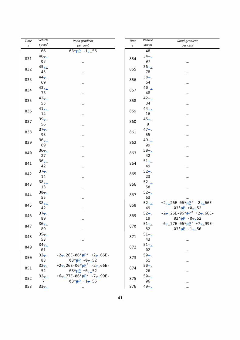
Figure 16

HILS method flow chart

A.9.2.2. Build and verification of the HILS system setup

The HILS system setup shall be constructed and verified in accordance with the provisions of paragraph A.9.3.

A.9.2.3. Build and verification of HV model

The reference HV model shall be replaced by the specific HV model for ap-proval representing the specified HD hybrid vehicle/powertrain and after en-abling all other HILS system parts, the HILS system shall meet the provi-sions of paragraph A.9.5. to give the confirmed representative HD hybrid vehicle operation conditions.

A.9.2.4. Creation of the Hybrid Engine Cycle

41

As part of the procedure for creation of the hybrid engine test cycle, the hy-brid system power shall be determined in accordance with the provisions of paragraph A.9.6.3. or A.10.4. to obtain the hybrid system rated power. The hybrid engine test cycle (HEC) shall be the result of the HILS simulated run-ning procedure in accordance with the provisions of paragraph A.9.6.4.

A.9.2.5. Exhaust emission test

The exhaust emission test shall be conducted in accordance with paragraphs 6 and 7.

A.9.2.6. Data collection and evaluation

A.9.2.56.1. Emission relevant data

All data relevant for the pollutant emissions shall be recorded in accordance with paragraphs 7.6.6. during the engine emission test run.

If the predicted temperature method in accordance with paragraph A.9.6.2.18. is used, the temperatures of the elements that influence the hybrid control shall be recorded.

A.9.2.6.2. Calculation of hybrid system work

The hybrid system work shall be determined over the test cycle by synchron-ously using the hybrid system rotational speed and torque values at the wheel hub (HILS chassis model output signals in accordance with paragraph A.9.7.3.) from the valid HILS simulated run of paragraph A.9.6.4. to calcu-late instantaneous values of hybrid system power. Instantaneous power val-ues shall be integrated over the test cycle to calculate the hybrid system work from the HILS simulated running Wsys_HILS (kWh). Integration shall be carried out using a frequency of 5 Hz or higher (10 Hz recommended) and include allonly positive power values in accordance with paragraph A.9.7.3.

The hybrid system work Wsys shall be calculated as follows:

(a) Cases where Wact < Weng_HILS:

(Eq. 107)

W sys=W sysHILS×W act/W eng HILS

×( 10.95 )

2

(107)

(b) Cases where Wact ≥ Weng_HILS

(Eq. 108)

W sys=W sysHILS×( 1

0.95 )2

(108)

Where:

Wsys : Hybridis the hybrid system work (, kWh)

Wsys_HILS : Hybridis the hybrid system work from the final HILS simulated run (, kWh)

Wact : Actualis the actual engine work in the HEC test (, kWh)

Weng_HILS : Engineis the engine work from the final HILS simulated run (, kWh)

42

All parameters shall be reported.

A.9.2.6

43

A.9.2.6.3. Validation of predicted temperature profile

In case the predicted temperature profile method in accordance with para-graph A.9.6.2.18. is used, it shall be proven, for each individual temperature of the elements that affect the hybrid control, that this temperature used in the HILS run is equivalent to the temperature of that element in the actual HEC test.

The method of least squares shall be used, with the best-fit equation having the form:

y = a1x + a0 (XX)

Where:

y is the predicted value of element temperature, °C

a1 is the slope of the regression line

x is the measured reference value of element temperature, °C

a0 is the y-intercept of the regression line

The standard error of estimate (SEE) of y on x and the coefficient of determ-ination (r²) shall be calculated for each regression line.

This analysis shall be performed at 1 Hz or greater. For the regression to be considered valid, the criteria of Table XXX shall be met.

Table XXXTolerances for temperature profiles

Element temperature

Standard error of estimate (SEE) of y on x

maximum 5 per cent of maximum meas-ured element temperature

Slope of the regression line, a1

0.95 to 1.03

Coefficient of determina-tion, r²

minimum 0.970

y-intercept of the regres-sion line, a0

maximum 10 per cent of minimum measured element temper-ature

A.9.2.7. Calculation of specific emissions for hybrids

The specific emissions egas or ePM (g/kWh) shall be calculated for each indi-vidual component as follows:

(Eq.

❑❑❑

(109)

Where:

e is the specific emission (, g/kWh)

m is the mass emission of the component (, g/test)

44

Wsys is the cycle work as determined in accordance with paragraph A.9.2.5.1. (6.2., kWh)

The final test result shall be a weighted average from cold start test and hot start test in accordance with the following equation:

(Eq. 110)

e=(0.14 ×mcold)+(0.86 × mhot)

(0.14 ×W sys ,cold)+(0.86 × W sys , hot) (110)

Where:

mcold is the mass emission of the component on the cold start test (, g/test)

mhot is the mass emission of the component on the hot start test (, g/test)

Wsys,cold is the hybrid system cycle work on the cold start test (, kWh)

Wsys,hot is the hybrid system cycle work on the hot start test (, kWh)

If periodic regeneration in accordance with paragraph 6.6.2. applies, the re-generation adjustment factors kr,u or kr,d shall be multiplied with or be added to, respectively, the specific emission result e as determined in equations 109 and 110.

A.9.3. Build and verification of hilsHILS system setup

A.9.3.1 General introduction

The build and verification of the HILS system setup procedure is outlined in Figure 17 below and provides guidelines on the various steps that shall be ex-ecuted as part of the HILS procedure.

Figure 17HILS system build and verification diagram

45

The HILS system shall consist of, as shown in Figure 18, all required HILS hardware, a HV model and its input parameters, a driver model and the test cycle as defined in Annex 1.b., as well as the hybrid ECU(s) of the test motor vehicle (hereinafter referred to as the "actual ECU") and its power supply and required interface(s). The HILS system setup shall be defined in accordance with paragraph A.9.3.2. through A.9.3.6. and considered valid when meeting the criteria of paragraph A.9.3.7. The reference HV model (paragraph A.9.4.) and HILS component library (paragraph A.9.7.) shall be applied in this pro-cess.

Figure 18:

Outline of HILS system setup

A.9.3.2. HILS hardware

The HILS hardware shall contain all physical systems to build up the HILS system, but excludes the actual ECU(s).

The HILS hardware shall have the signal types and number of channels that are required for constructing the interface between the HILS hardware and the actual ECU(s), and shall be checked and calibrated in accordance with the procedures of paragraph A.9.3.7. and using the reference HV model of para-graph A.9.4.

A.9.3.3. HILS software interface

The HILS software interface shall be specified and set up in accordance with the requirements for the (hybrid) vehicle model as specified in paragraph A.9.3.5. and required for the operation of the HV model and actual ECU(s). It

46

shall be the functional connection between the HV model and driver model to the HILS hardware. In addition, specific signals can be defined in the inter-face model to allow correct functional operation of the actual ECU(s), e.g. ABS signals.

The interface shall not contain key hybrid control functionalities as specified in paragraph A.9.3.4.1.

A.9.3.4. Actual ECU(s)

The hybrid system ECU(s) shall be used for the HILS system setup. In case the functionalities of the hybrid system are performed by multiple controllers, those controllers may be integrated via interface or software emulation. However, the key hybrid functionalities shall be included in and executed by the hardware con-troller(s) as part of the HILS system setup.

A.9.3.4.1. Key hybrid functionalities

Reserved.

The key hybrid functionality shall contain at least the energy management and power distribution between the hybrid powertrain energy converters and the RESS.

A.9.3.5. Vehicle model

A vehicle model shall represent all relevant physical characteristics of the (heavy-duty) hybrid vehicle/powertrain to be used for the HILS system. The HV model shall be constructed by defining its components in accordance with paragraph A.9.7.

Two HV models are required for the HILS method and shall be constructed as follows:

(a) A reference HV model in accordance with its definition in paragraph A.9.4. shall be used for a SILS run using the HILS system to confirm the HILS system performance.

(b) A specific HV model defined in accordance with paragraph A.9.5. shall qualify as the valid representation of the specified heavy-duty hybrid powertrain. It shall be used for determination of the hybrid en-gine test cycle in accordance with paragraph A.9.6. as part of this HILS procedure.

A.9.3.6. Driver model

The driver model shall contain all required tasks to drive the HV model over the test cycle and typically includes e.g. accelerator and brake pedal signals as well as clutch and selected gear position in case of a manual shift transmis-sion.

The driver model tasks may be implemented as a closed-loop controller or lookup tables as function of test time.

A.9.3.7. Operation check of HILS system setup

The operation check of the HILS system setup shall be verified through a SILS run using the reference HV model (paragraph A.9.4.) on the HILS sys-temA.9.

Linear regression of the calculated output values of the reference HV model SILS run on the provided reference values (paragraph A.9.4.4.) shall be per-

47

formed. The method of least squares shall be used, with the best-fit equation having the form:

y = a1x + a0 (111)

Where:

y =is the actual HILS value of the signal

x =is the measured reference value of the signal

a =

a1 is the slope of the regression line

b =

a0 is the y-intercept value of the regression line

For the HILS system setup to be considered valid, the criteria of Table 10 shall be met.

In case the programming language for the HV model is other than Matlab®/Simulink®, the confirmation of the calculation performance for the HILS sys-tem setup shall be proven using the specific HV model verification in accord-ance with paragraph A.9.5.

Table 10Tolerances for HILS system setup operation check

Verifica- Criteriaslope, a

a1

y-intercept, ba0

coefficient of determination,r2

Vehicle

0.9995 –to 1.0005 ±0.05 % or less of the maximum value

minimum 0.995 or higher

ICE speedICE torqueEM speedEM torqueREESS voltageREESS currentREESS SOC

A.9.4. Reference hybrid vehicle model

A.9.4.1. General introduction

The purpose of the reference HV model shall be the use in confirmation of the calculation performance (e.g. accuracy, frequency) of the HILS system setup (paragraph A.9.3.) by using a predefined hybrid topology and control functionality for verifying the corresponding HILS calculated data against the expected reference values.

A.9.4.2 Reference HV model description

The reference HV model has a parallel hybrid powertrain topology consisting of following components, as shown in Figure 19, and includes its control strategy:

(a) Internal Combustion Engine

48

(b) Clutch

(c) Battery

(d) Electric Motor

(e) Mechanical gearing (for connection of EM between clutch and trans-mission)

(f) Shift transmission

(g) Final gear

(h) Chassis, including wheels and body

The reference HV model is available as part of the HILS library available at http://www.unece.org/trans/main/wp29/wp29wgs/wp29gen/wp29glob_registry.html. at the GTR No.4 addendum.

The reference HV model is named "reference_hybrid_vehicle_model.mdl" and its parameter files as well as the SILS run output data are available at the following directory in the HILS library: "<root>\HILS_GTR\Vehicles\ReferenceHybridVehicleModel" (and all of its subdirectories).

Figure 19Reference HV model powertrain topology

A.9.4.3. Reference HV model input parameters

All component input data for the reference HV model is predefined and loc-ated in the model directory:

"<root>\HILS_GTR\Vehicles\ReferenceHybridVehicleModel\ParameterData".

This directory contains files with the specific input data for:

(a) The (internal combustion) engine model : "para_engine_ref.m"

(b) The clutch model : "para_clutch_ref.m"

(c) The battery model : "para_battery_ref.m"

(d) The electric machine model : "para_elmachine_ref.m"

(e) The mechanical gearing : "para_mechgear_ref.m"

49

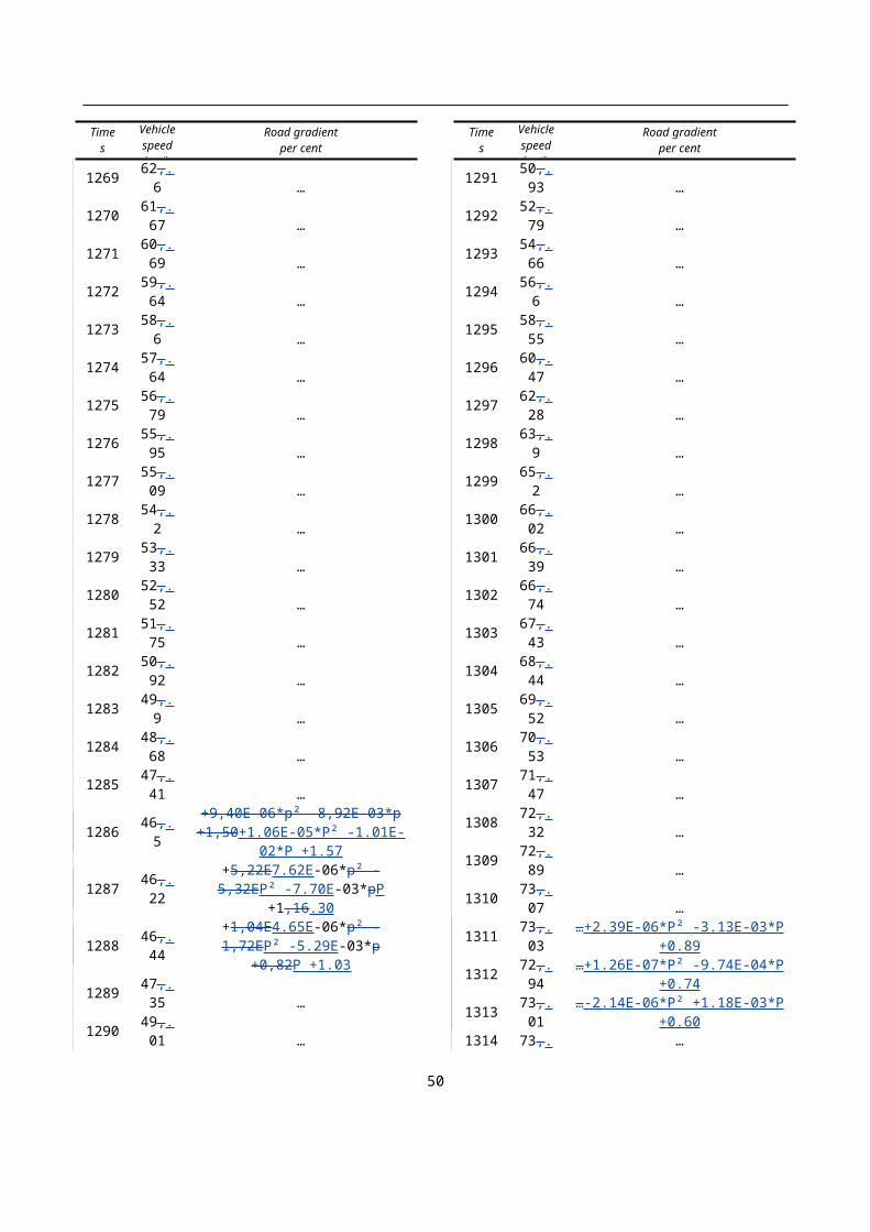
http://www.unece.org/trans/main/wp29/wp29wgs/wp29gen/wp29glob_registry.html

(f) The (shift) transmission model : "para_transmission_ref.m"

(g) The final gear model : "para_finalgear_ref.m"

(h) The vehicle chassis model : "para_chassis_ref.m"

(i) The test cycle : "para_drivecycle_ref.m"

(j) The hybrid control strategy : "ReferenceHVModel_Input.mat"

The hybrid control strategy is included in the reference HV model and its control parameters for the engine, electric machine, clutch and so on are defined in lookup tables and stored in the specified file.

A.9.4.4. Reference HV output parameters

A selected part of the test cycle as defined in Annex 1.b. covering the first 140 seconds is used to perform the SILS run with the reference HV model. The calculated data for the SILS run using the HILS system shall be recorded with at least 5 Hz and be compared to the reference output data stored in file "ReferenceHVModel_Output.mat" available in the HILS library directory:

"<root>\HILS_GTR\Vehicles\ReferenceHybridVehicleModel\SimResults".

The SILS run output data shall be rounded to the same number of significant digits as specified in the reference output data file and shall meet the criteria listed in Table 10.

A.9.5. Build and verification of the specific HV model

A.9.5.1. Introduction

This procedure shall apply as the build and verification procedure for the spe-cific HV model as equivalent representation of the actual hybrid powertrain to be used with the HILS system setup in accordance with paragraph A.9.3.

A.9.5.2. General procedure

The diagram of Figure 20 provides an overview of the various steps towards the verified specific HV model.

Figure 20

Specific HV model build and verification flow diagram

50

A.9.5.3. Cases requiring verification of specific HV model and HILS system

The verification aims at checking the operation and the accuracy of the simu-lated running of the specific HV model. The verification shall be conducted when the equivalence of the HILS system setup or specific HV model to the test hybrid powertrain needs to be confirmed.

In case any of following conditions applies, the verification process in ac-cordance with paragraph A.9.5.4. through A.9.5.8. shall be required:

(a) The HILS system including the actual ECU(s) is run for the first time, e.g. after changes to its hardware or actual ECU(s) calibration..

(b) The HV system layout has changed.

(c) ChangesStructural changes are made to component models (e.g. struc-tural change, larger or smaller number of model input parameters)..

(d) Different use of model component (e.g. manual to automated trans-mission).

(e) Response delay times or time constants of (e.g. internal combustion engine or electric motor, gear shifting and so on) models are modified.

(f) Changes are made to the interface model. that have relevant impact on the hybrid functionality.

(gf) A manufacturer specific component model is used for the first time.

The type approval or certification authority may conclude that other cases ex-ist and request verification.

The HILS system and specific HV model including the need for verification shall be subject to approval by the type approval or certification authority. All deviations that affect the above mentioned verification criteria shall be provided to the type approval or certification authority along with the ra-tionale for justification and all appropriate technical information as proof therefore., e.g. the deviation by changes to the HILS system hardware, modi-fication of the response delay times or time constants of models. The tech-nical information shall be based on calculations, simulations, estimations, de-scription of the models, experimental results and so on.

A.9.5.4. Actual hybrid powertrain test

A.9.5.4.1 Specification and selection of the test hybrid powertrain

Reserved.

The test hybrid powertrain shall be the parent hybrid powertrain. If a new hy-brid powertrain configuration is added to an existing family in accordance with paragraph 5.3.2., which becomes the new parent powertrain, HILS model validation is not required.

A.9.5.4.2. Test procedure

The verification test using the test hybrid powertrain (hereinafter referred to as the "actual powertrain test") which serves as the standard for the HILS sys-tem verification shall be conducted by either of the test methods described in paragraphs A.9.5.4.2.1. to A.9.5.4.2.2.

Provisions concerning

51

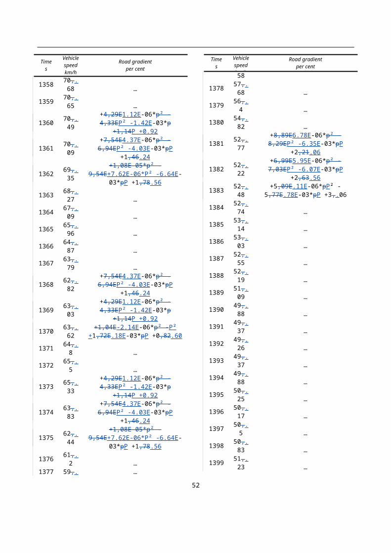
A.9.5.4.2.1. Powertrain dynamometer test

The test shall be carried out in accordance with the provisions of paragraphs A.10.3. and A.10.5. in order to determine the measurement ofitems specified in paragraph A.9.5.4.4.

The measurement of the exhaust emissions may be omitted.

A.9.5.4.2.1. Powertrain dynamometer test

Reserved.

A.9.5.4.2.2. Chassis dynamometer test

Reserved.A.9.5.4.2.2.1. General introduction

The test shall be carried out on a chassis dynamometer with adequate charac-teristics to perform the test cycle specified in Annex 1.b.

The dynamometer shall be capable of performing an (automated) coastdown procedure to determine and set the correct road load values as follows:

(1) the dynamometer shall be able to accelerate the vehicle to a speed above the highest test cycle speed or the maximum vehicle speed, whichever is the lowest.

(2) run a coastdown

(3) calculate and subtract the Dynomeasured load coefficients from the Dynot-

arget coefficients

(4) adjust the Dynosettings

(5) run a verification coastdown

The dynamometer shall automatically adjust its Dynosettings by repeating steps (1) through (5) above until the maximum deviation of the Dynomeasured load curve is less than 5 per cent of the Dynotarget load curve for all individual speeds within the test range.

The Dynotarget road load coefficients are defined as A, B and C and the corres-ponding road load is calculated as follows:

F roadload=A+B × v+C × v❑2 (112)

Where:

Froadload is the dynamometer road load, N

Dynomeasured are the Am, Bm and Cm dynamometer coefficients calculated from the dynamometer coastdown run

Dynosettings are the Aset, Bset and Cset coefficients which command the road load simulation done by the dynamometer

Dynotarget are the Atarget, Btarget and Ctarget dynamometer target coefficients in accordance with paragraphs A.9.5.4.2.2.2. through A.9.5.4.2.2.6.

Prior to execution of the dynamometer coastdown procedure, the dynamo-meter shall have been calibrated and verified in accordance with the dynamo-meter manufacturer specifications. The dynamometer and vehicle shall be preconditioned in accordance with good engineering judgement to stabilize the parasitic losses.

52

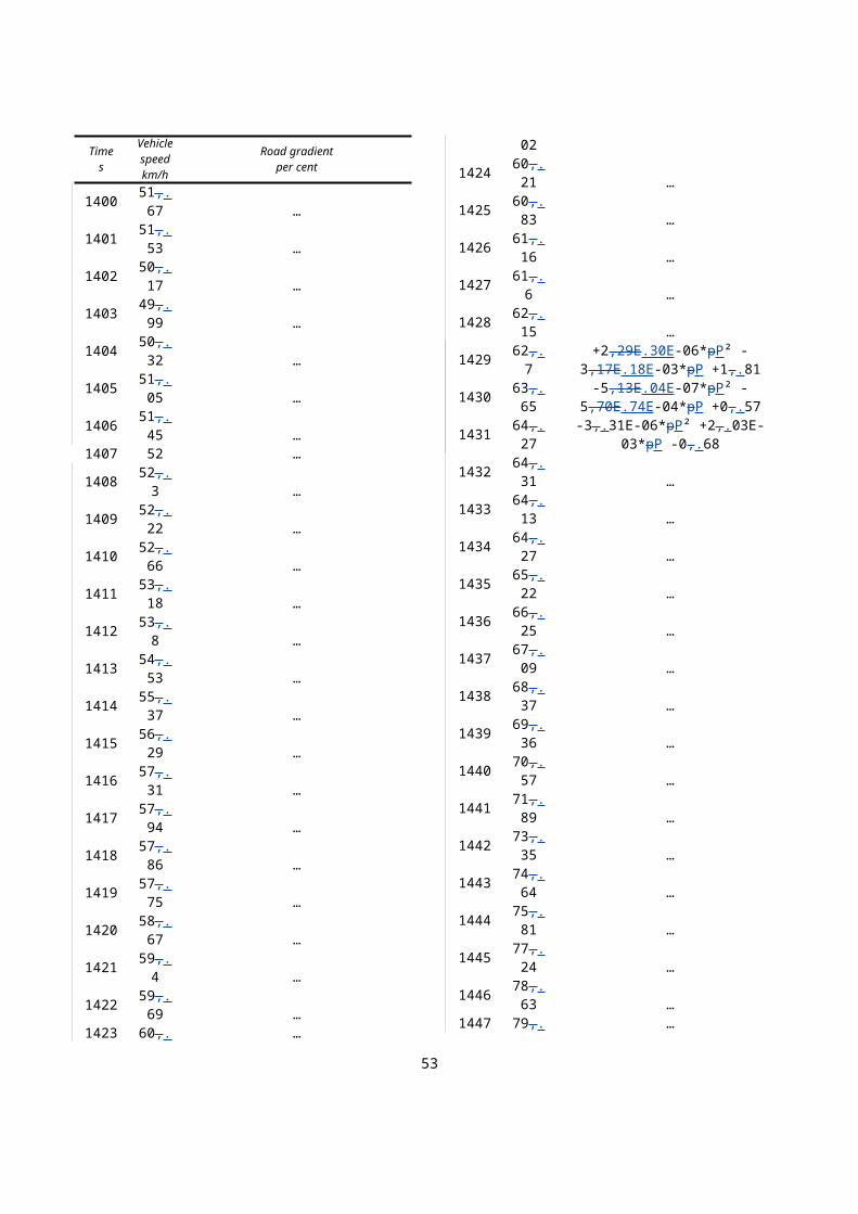
All measurement instruments shall meet the applicable linearity requirements of A.9.8.3.

All modifications or signals required to operate the hybrid vehicle on the chassis dynamometer shall be documented and reported to the type approval authorities or certification agency.

A.9.5.4.2.2.2. Vehicle test mass

The vehicle test mass mvehicle shall be calculated using the hybrid system rated power Prated, as specified by the manufacturer for the actual test hybrid power-train, as follows:

mvehicle=15.1 × Prated1.31 (113)

Where:

mvehicle is the vehicle test mass, kg

Prated is the hybrid system rated power, kW

A.9.5.4.2.2.3. Air resistance coefficients

The vehicle frontal area Afront (m2 ) shall be calculated as function of vehicle test mass in accordance with A.9.5.4.2.2.2. using following equations:

(a) for mvehicle ≤ 18050 kg :

A front=−1.69 ×10−8× mvehicle2 +6.33 ×10−4 ×mvehicle+1.67 (114)

or

(b) for mvehicle > 18050 kg :

A front=7.59m2 (115)

The vehicle air drag resistance coefficient Cdrag (-) shall be calculated as fol-lows:

Cdrag=3.62 × (0.00299 × A front−0.000832) × g

0.5 × ρa× A front

(116)

Where:

g is the gravitational acceleration with a fixed value of 9.80665 m/s2

ρa is the air density with a fixed value of 1.17 kg/m3

A.9.5.4.2.2.4. Rolling resistance coefficient

The rolling resistance coefficient (-) shall be calculated as follows:

f roll=0.00513+ 17.6mvehicle

(118)

Where:

53

mvehicle is the test vehicle mass in accordance with paragraph A.9.5.4.2.2.2., kg

A.9.5.4.2.2.5. Rotating inertia

The inertia setting used by the dynamometer to simulate the vehicle inertia shall equal the vehicle test mass in accordance with paragraph A.9.5.4.2.2.2. No correction shall be carried out to account for axle inertias in the dynamo-meter load settings.

A.9.5.4.2.2.6. Dynamometer settings

The road load at a certain vehicle speed v shall be calculated using equation 112.

The A, B and C coefficients are as follows:

A=mvehicle × g × f roll (X)

B = 0 (X)

C=12

× ρa×Cdrag × A front (X)

Where:

v is the vehicle speed, m/s

mvehicle is the vehicle test mass in accordance with paragraph A.9.5.4.2.2.2., kg

froll is the rolling resistance coefficient specified in accordance with paragraph A.9.5.4.2.2.4.

g is the gravitational acceleration as specified in accordance with paragraph A.9.5.4.2.2.3., m/s2

ρa is the ambient air density as specified in accordance with para-graph A.9.5.4.2.2.3., kg/m3

Cdrag is the vehicle air drag coefficient as specified in accordance with paragraph A.9.5.4.2.2.3.

Afront is the vehicle frontal area as specified in accordance with para-graph A.9.5.4.2.2.3., m2

A.9.5.4.2.2.7. Dynamometer road load simulation mode

The dynamometer shall be operated in a mode that it simulates the vehicle in-ertia and the road load curve defined by the Dynosetting coefficients.

The dynamometer shall be capable of correctly implementing road gradients as defined in accordance with the test cycle in Annex 1.b. so that A effect-ively satisfies:

A=mvehicle × g × f roll× cos ( αroad )+mvehicle × g ×sin ( αroad ) (X)

α road=atan (α road /100 ) (X)

Where:

αroad is the road gradient, rad

54

αroad_pct is the road gradient as specified in Annex 1.b., per cent

A.9.5.4.3. Test conditions

A.9.5.4.3.1. Test cycle run

The test shall be conducted as a time-based test by running the full test cycle as defined in Annex 1.b. using the hybrid system rated power in accordance with the manufacturer specification.

A.9.5.4.3.2. Various system settings

The following conditions shall be met, if applicable:

(1) The road gradient shall not be fed into the ECU (level ground posi-tion) or inclination sensor should be disabled

(2) The ambient test conditions shall be between 20°C and 30°C

(3) Ventilation systems with adequate performance shall be used to con-dition the ambient temperature and air flow condition to represent on-road driving conditions.

(4) Continuous brake systems shall not be used or shall be switched off if possible

(5) All auxiliary or PTO systems shall be turned off or their power con-sumption measured. If measurement is not possible, the power con-sumption shall be based on calculations, simulations, estimations, ex-perimental results and so on. Alternatively, an external power supply for 12/24V systems may be used.

(6) Prior to test start, the test powertrain may be key-on, but not enabling a driving mode, so that data communication for recording may be pos-sible. At test start, the test powertrain shall be fully enabled to the driving mode.

(7) The chassis dynamometer roller(s) shall be clean and dry. The driven axle load shall be sufficient to prevent tire slip on the chassis dynamo-meter roller(s). Supplementary ballast or lashing systems to secure sufficient axle load may be applied.

(8) If the desired deceleration of the test cycle cannot be achieved by braking within the allowable errors in accordance with paragraph A.9.5.4.3.3., e.g. a heavy vehicle with one axle on the chassis dy-namometer roller(s), the chassis dynamometer may assist decelerating the vehicle. This may result in a modification of the applied road gradient as specified in accordance with Annex 1.b. during these de-celerations.

(9) Preconditioning of test systems:

For cold start cycles, the systems shall be soaked so that the system temperatures are between 20°C and 30°.

A warm start cycle shall be preconditioned by running of the complete test cycle in accordance with Annex 1.b. followed by a 10 minute (hot) soak.

A.9.5.4.3.3. Validation of vehicle speed

The allowable errors in speed and time during the actual powertrain test shall be, at any point during each running mode, within ±4.0 km/h in speed and

55

±2.0 second in time as shown with the coloured section in Figure 21. Moreover, if deviations are within the tolerance corresponding to the setting items posted in the left column of Table 11, they shall be deemed to be within the allowable errors. The duration of deviations at gear change operation as specified in accordance with paragraph A.9.5.8.1. shall not be included in the total cumulative time. In addition, this provision on error duration shall not apply in case the demanded accelerations and speeds are not obtained during periods where the accelerator pedal is fully depressed (maximum perform-ance shall be requested from hybrid powertrain).

Table 11Tolerances for vehicle speed deviations in chassis dynamometer test

Setting item T

1. Tolerable time range for one deviation < ±2.0

2. Tolerable time range for the total cumulative value of (absolute) deviations

< 2.0

3. Tolerable speed range for one deviation < ±4.0

Figure 21Tolerances for speed deviation and duration during chassis dynamometer test

A.9.5.4.3.4. Test data analysis

The testing shall allow for analysing the measured data in accordance with the following two conditions:

(a) Selected part of test cycle, defined as the period covering the first 140 seconds;

56

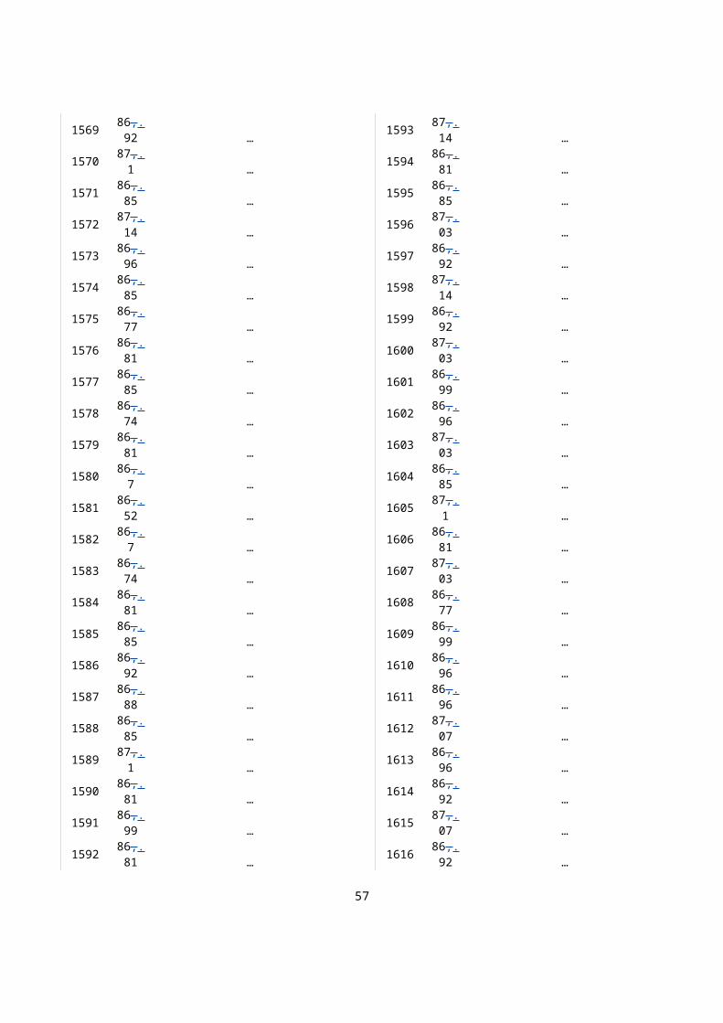
(b) The full test cycle.

A.9.5.4.4. Measurement items

For all applicable components, at least the following items shall be recorded using dedicated equipment and measurement devices (preferred) or ECU data (e.g. using CAN signals). The accuracy of measuring devices shall be in ac-cordance with the provisions of paragraphs 9.2. and A.8.8.3. The sampling frequency shall be 5 Hz or higher. Data so obtained shall become the actu-ally-measured data for the HILS system verification (hereinafter referred to as the "actually-measured verification values"):using CAN signals) in order to enable the verification:

(a) Hybrid system speed (min-1), hybrid system torque (Nm), hybrid sys-tem power (kW);

(b) SetpointTarget and actual vehicle speed (km/h);

(cb) Quantity of driver manipulation of the vehicle (typically accelerator, brake, clutch and shift operation signals, and alike) or quantity of ma-nipulation on the engine dynamometer (throttle valve opening angle). All signals shall be in units as applicable to the system and suitable for conversion towards use in conversion and interpolation routines;

(dc) Engine speed (min-1),) and engine command values (-, %,per cent, Nm, units as applicable);

) or, alternatively, fuel injection value (e.g. mg/str);

(d) Electric motor speed (min-1), torque command value (-, %,per cent, Nm as applicable) (or their respective physically equivalent signals for non-electric energy converters);

(fe) (Rechargeable) energy storage system power (kW), voltage (V) and current (A) (or their respective physically equivalent signals for non-electric RESS).

The accuracy of measuring devices shall be in accordance with the provisions of paragraphs 9.2. and A.9.8.3.

The sampling frequency for all signals shall be 5 Hz or higher.

The recorded CAN signals in (d) and (e) shall be used for post processing us-ing actual speed and the CAN (command) value (e.g. fuel injection amount) and the specific characteristic component map as obtained in accordance with paragraph A.9.8. to obtain the value for verification by means of the Hermite interpolation procedure (in accordance with appendix 1 to Annex 9).

All recorded and post process data so obtained shall become the actually-measured data for the HILS system verification (hereinafter referred to as the "actually-measured verification values").

A.9.5.5. Specific HV model

The specific HV model for approval shall be defined in accordance with A.9.3.5.(b) and its input parameters defined in accordance with A.9.5.6.

A.9.5.6. Specific HV model verification input parameters

A.9.5.6.1. General introduction

Input parameters for the applicable specific HV model components shall be defined as outlined in paragraphs A.9.5.6.2. to A.9.5.6.16.

57

A.9.5.6.2. Engine characteristics

The parameters for the engine torque characteristics shall be the table data obtained in accordance with paragraph A.9.8.3. However, values equivalent to or lower than the minimum engine revolution speed may be added.

A.9.5.6.3. Electric machine characteristics

The parameters for the electric machine torque and electric power consump-tion characteristics shall be the table data obtained in accordance with para-graph A.9.8.4. However, characteristic values at a revolution speed of 0 rpm may be added.

A.9.5.6.4. Battery characteristics

A.9.5.6.4.1. Resistor based model

The parameters for the internal resistance and open-circuit voltage of the bat-tery model shall be the input data obtained in accordance with paragraph A.9.8.5.1.

A.9.5.6.4.2. RC-circuit based model

The parameters for the RC-circuit battery model shall be the input data ob-tained in accordance with paragraph A.9.8.5.2.

A.9.5.6.5. Capacitor characteristics

The parameters for the capacitor model shall be the data obtained in accord-ance with paragraph A.9.8.5.36.

A.9.5.6.6. Vehicle test mass and curb mass

The vehicle test mass mvehicle shall be calculated using the hybrid system rated power Prated,defined as specified by the manufacturer for the actual hybrid powertrain test hybrid powertrain, as follows:in accordance with paragraph A.9.5.4.2.2.2.

(Eq. 114)

A.9.5.6.7. Air resistance coefficients

The vehicle frontal area Afrontair resistance coefficients shall be calculateddefined as function of vehiclefor the actual hybrid powertrain test mass in accordance with paragraph A.9.5. (Eq. 117)

Where:

g : gravitational acceleration with a fixed value of 9.80665 (m/s2)

ρa : air density with a fixed value of 1.17 kg/m

A.9.5.6.8. Rolling resistance coefficient

The rolling resistance coefficientcoefficients shall be calculateddefined as (Eq. 118)

Where:

mvehicle :for the actual hybrid powertrain test vehicle mass (kg) in accordance with paragraph A.9.5.6.7.4.2.2.4.

58

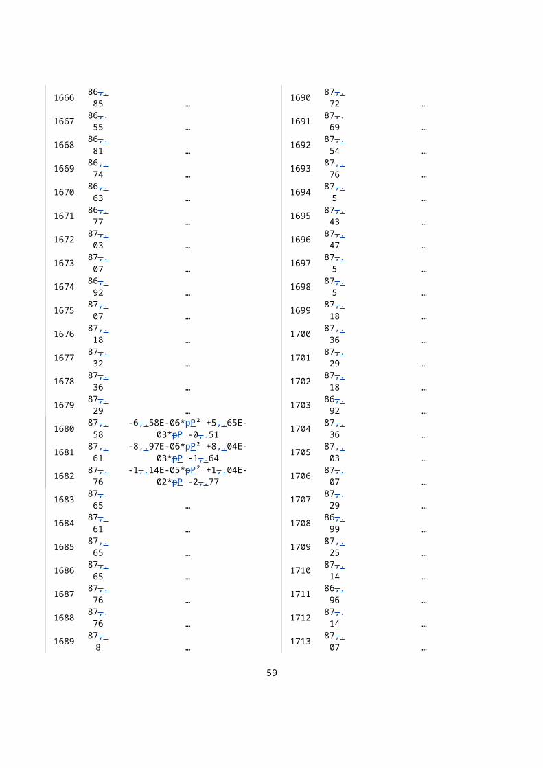
A.9.5.6.9. Wheel radius

The wheel radius shall be the manufacturer specified value as used in the ac-tual test hybrid powertrain.

A.9.5.6.10. Final gear ratio

The final gear ratio shall be the manufacturer specified ratio representative for the actual test hybrid powertrain.

A.9.5.6.11. Transmission efficiency

The transmission efficiency shall be the manufacturer specified value for the transmission of the actual test hybrid powertrain.

A.9.5.6.12. Clutch maximum transmitted torque

For the maximum transmitted torque of the clutch and the synchronizer, the design value specified by the manufacturer shall be used.

A.9.5.6.13. Gear change period

The gear-change periods for a manual transmission shall be the actual test values.

A.9.5.6.14. Gear change method

Gear positions at the start, acceleration and deceleration during the verifica-tion test shall be the respective gear positions in accordance with the spe-cified methods for the types of transmission listed below:

(a) For manual shift transmission: gear positions are defined by actual test values.

(b) For automated shift transmission (AMT) or automatic gear box (AT): gear positions are generated by the shift strategy of the actual trans-mission ECU during the HILS simulation run and shall not be the re-corded values from the actual test.

A.9.5.6.15. Inertia moment of rotating sections

The inertia for all rotating sections shall be the manufacturer specified values representative for the actual test hybrid powertrain.

A.9.5.6.16. Other input parameters

All other input parameters shall have the manufacturer specified value repres-entative for the actual test hybrid powertrain.

A.9.5.7. Specific HV model HILS run for verification

A.9.5.7.1. Method for HILS running

Use the HILS system pursuant to the provisions of paragraph A.9.3. and in-clude the specific HV model for approval with its verification parameters (paragraph A.9.5.6.) to perform a simulated running pursuant to paragraph A.9.5.7.2. and record the calculated HILS data related to paragraph A.9.5.4.4. The data so obtained is the HILS simulated running data for HILS system verification (hereinafter referred to as the "HILS simulated running values").

Auxiliary loads measured in the actual test hybrid powertrain may be used as input to the auxiliary load models (either mechanical or electrical).

A.9.5.7.2. Running conditions

59

The HILS running test shall be conducted as one or two runs allowing for both of the following two conditions to be analysed (see Figure 21):

(a) Selected part of test cycle shall cover the first 140 seconds of the test cycle as defined in Annex 1.b. for which the road gradient are calcu-lated using the manufacturer specified hybrid system rated power also applied for the actual powertrain test. The driver model shall output the recorded values as obtained in the actual hybrid powertrain test (paragraph A.9.5.4.) to actuate the specific HV model.

(b) The full test cycle as defined in Annex 1.b. for which the road gradi-ents are calculated using the manufacturer specified hybrid system rated power also applied for the actual hybrid powertrain test. The driver model shall output all relevant signals to actuate the specific HV model based on either the reference test cycle speed or the actual vehicle speed as recorded in accordance with paragraph A.9.5.4.

IfIf the manufacturer declares that the resulting HEC engine operating condi-tions for cold and hot start cycles are different, both the (e.g. due to the ap-plication of a specific cold and hot start cyclesstrategy), a verification shall be verified.carried out by use of the predicted temperature method in accord-ance with paragraphs A.9.6.2.18. and A.9.2.6.3.. It shall then be proven that the predicted temperature profile of the elements affecting the hybrid control operation is equivalent to the temperatures of those elements measured dur-ing the HEC exhaust emission test run.

In order to reflect the actual hybrid powertrain test conditions (e.g. temperat-ures, RESS available energy content), the initial conditions shall be the same as those in the actual test and applied to component parameters, interface parameters and so on as needed for the specific HV model.

60

Figure 21Flow diagram for verification test HILS system running with specific HV model

A.9.5.8. Validation statistics for verification of specific HV model for approval

A.9.5.8.1. Confirmation of correlation on the selected part of the test cycle

Correlation between the actually-measured verification values (as reference values) and the HILS simulated running values shall be verified for the selec-ted test cycle part in accordance with paragraph A.9.5.7.2.(a). Table 11 shows the requirements for the tolerance criteria between those values. Here, the data during gear change periods may be omitted for this regression ana-lysis, but no more than a period of 2.0 seconds per gear change.

The following points may be omitted from the regression analysis:

(a) the gear change period

(b) 1.0 second before and after the gear change period

A gear change period is defined from the actually-measured values as:

(1) for gear change systems that require the disengagement and engage-ment of a clutch system, the period from the disengagement of the clutch to the engagement of the clutch,

or

(2) for gear change systems that do not require the disengagement or en-gagement of a clutch system, the period from the moment a gear is disengaged to the moment another gear is engaged.

The omission of test points shall not apply for the calculation of the engine work.

61

Table 11Tolerances (for the selected part of the test cycle) for actually measured and HILS simulated running values for specific HV model verification

Vehicle and/or engine

Engine Electric Motor (or equivalent)

Electric Storage Device

(or equivalent) Speed Torque Power Torque Power Power

Coefficient of determination, r2

>0.97 >0.88 >0.88 >0.88 >0.88 0.88

A.9.5.8.2. Overall verification for complete test cycle

A.9.5.8.2.1. Verification items and tolerances

Correlation between the actually-measured verification values and the HILS simulated running values shall be verified for the full test cycle (in accord-ance with paragraph A.9.5.7.2.(b).). Here, the data during gear change peri-ods may be omitted for this regression analysis, but no more than a period of 2.0 seconds per gear change.

The following points may be omitted from the regression analysis:

(a) the gear change period

(b) 1.0 second before and after the gear change period

A gear change period is defined from the actually-measured values as:

(1) for gear change systems that require the disengagement and engage-ment of a clutch system, the period from the disengagement of the clutch to the engagement of the clutch,

or

(2) for gear change systems that do not require the disengagement or en-gagement of a clutch system, the period from the moment a gear is disen-gaged to the moment another gear is engaged.

The omission of test points shall not apply for the calculation of the engine work.

For the specific HV model to be considered valid, the criteria of Table 12 and those of paragraph A.9.5.8.1. shall be met.

Table 12 Tolerances (for full test cycle) for actually measured verification values and HILS simulated running values

Vehicle speed Engine

Positive engine work

Torque

Coefficient of determination, r2 > 0.97 > 0.88

Conversion ratio 0.97 < … < Y

Where:

Weng_HILS : Engineis the engine work in the HILS simulated running (, kWh)

62

Weng_test : Engineis the engine work in the actual powertrain test (, kWh)

Wsys_HILS : Hybrid system work in HILS simulated running (kWh)

Wsys_test : Hybrid system work in actual powertrain test (kWh)

A.9.5.8.2.2. Calculation method for verification items

The engine torque, power and the positive work shall be acquired by the fol-lowing methods, respectively, in accordance with the test data enumerated below:

(a) Actually-measured verification values in accordance with paragraph A.9.5.4.:

Methods that are technically valid, such as a method where the value is calculated from the operating conditions of the hybrid system (revolu-tion speed, shaft torque) obtained by the actual hybrid powertrain test, using the input/output voltage and current to/from the electric machine (high power) electronic controller, or a method where the value is calcu-lated by using the data such acquired pursuant the component test pro-cedures in paragraph A.9.8.

(b) HILS simulated running values in accordance with paragraph A.9.5.7:

A method where the value is calculated from the engine operating conditions (speed, torque) obtained by the HILS simulated running.

A.9.5.8.2.3. Tolerance of net energy change for RESS

The net energy changes in the actual hybrid powertrain test and that during the HILS simulated running shall satisfy the following equation:

|∆ EHILS−∆ Etest|/W eng HILS<0.01 (119)

Where:

ΔEHILS : Net is the net energy change of RESS during the HILS sim-ulated running (, kWh)

ΔEtest : Net is the net energy change of RESS during the actual powertrain test (, kWh)

Weng_HILS : Positiveis the positive engine work from the HILS simulated run (, kWh)

And where the net energy change of the RESS shall be calculated as follows in case of:

(a) Battery

(Eq. ❑❑ (120)

Where:

ΔAh : Electricityis the electricity balance obtained by integration of the battery current (, Ah )

Vnominal : Rated is the rated nominal voltage (, V)

(b) Capacitor

❑❑ (❑❑❑❑❑

❑) (121)

63

Where:

Ccap : Ratedis the rated capacitance of the capacitor (, F)

Uinit : Initialis the initial voltage at start of test (, V)

Ufinal : Finalis the final voltage at end of test (, V)

(c) Flywheel:

❑❑❑❑

❑

(❑❑❑❑❑

❑) (122)

Where:

Jflywheel : Flywheelis the flywheel inertia (, kgm2)

ninit : Initialis the initial speed at start of test (, min-1)

nfinal : Finalis the final speed at end of test (, min-1)

(d) Other RESS:

The net change of energy shall be calculated using physically equival-ent signal(s) as for cases (a) through (c) in this paragraph. This method shall be reported to the Type Approval Authorities or Certific-ation Agency.

A.9.5.8.2.4. Additional provision on tolerances in case of fixed point engine operation

In case of fixed point engine operating conditions (both speed and torque), the verification shall be valid when the criteria for vehicle speed, positive en-gine work and engine running duration (same criteria as positive engine work) are met.

A.9.6. Creation of the hybrid engine cycle


Using the verified HILS system setup with the specific HV model for ap-proval, the creation of the hybrid engine cycle shall be carried out in accord-ance with the provisions of paragraphs A.9.6.2 to A.9.6.5. Figure 22 provides a flow diagram of required steps for guidance in this process.

64

Figure 22

Flow diagram for Creation of the Hybrid Engine Cycle

A.9.6.2. HEC run input parameters for specific HV model

A.9.6.2.1 General introduction

The input parameters for the specific HV model shall be specified as outlined in paragraphs A.9.6.2.2. to A.9.6.2.16. such as to represent a generic heavy-duty vehicle with the specific hybrid powertrain, which is subject to ap-proval. All input parameter values shall be rounded to 4 significant digits (e.g. x.xxxEyy in scientific representation).

A.9.6.2.2. Engine characteristics

The parameters for the engine torque characteristics shall be the table data obtained in accordance with paragraph A.9.8.3. However, values equivalent to or lower than the minimum engine revolution speed may be added. In ad-dition, the engine model accessory torque map shall not be used at the time of the approval test.

65

A.9.6.2.3. Electric machine characteristics

The parameters for the electric machine torque and electric power consump-tion characteristics shall be the table data obtained in accordance with para-graph A.9.8.4. However, characteristic values at a revolution speed of 0 rpm may be added.

A.9.6.2.4. Battery characteristics

A.9.6.2.4.1. Resistor based battery model

The input parameters for the internal resistance and open-circuit voltage of the resistor based battery model shall be the table data obtained in accordance with paragraph A.9.8.5.1.

A.9.6.2.4.2. RC-circuit based battery model

The parameters for the RC-circuit battery model shall be the data obtained in accordance with paragraph A.9.8.5.2.

A.9.6.2.5. Capacitor characteristics

The parameters for the capacitor model shall be the data obtained in accord-ance with paragraph A.9.8.6.

A.9.6.2.6. Vehicle test mass and curb mass

The vehicle test mass shall be calculated as function of the system rated power (A.10.as declared by the manufacturer) in accordance with equation 112.

The vehicle curb mass shall be calculated using equations 113 and 114.

A.9.6.2.7. Vehicle frontal area and air drag coefficient

The vehicle frontal area shall be calculated using equation 115 and 116 using the test vehicle mass in accordance with paragraph A.9.6.2.6.

The vehicle air drag resistance coefficient shall be calculated using equation 117 and the test vehicle mass in accordance with paragraph A.9.6.2.6.

A.9.6.2.8. Rolling resistance coefficient

The rolling resistance coefficient shall be calculated by equation 118 using the test vehicle mass in accordance with paragraph A.9.6.2.6.


The wheel radius shall be defined as 0.40 m or a manufacturer specified value, whichever. In case a manufacturer specified value is used, the wheel radius that represents the worst case with regard to the exhaust emissions shall be applied.

A.9.6.2.10. Final gear ratio and efficiency

The efficiency shall be set to 0.95.

The final gear ratio shall be defined in accordance with the provisions for the specified HV type:

(a) For parallel HV when using the standardized wheel radius, the final gear ratio shall be calculated as follows:

❑❑❑❑

❑❑

(❑❑❑❑❑❑❑❑ )❑❑

❑❑ (123)

66

Where:

rgear_high : is the ratio of highest gear number for powertrain trans-mission (-)

rwheel : is the dynamic tire radius (m) in accordance with para-graph A.9.6.2.9.., m

vmax : is the maximum vehicle speed with a fixed value of 87 km/h

nlo, nhi, nidle, npref : are the reference engine speeds in accord-ance with paragraph 7.4.6.

(b) For parallel HV when using a manufacturer specified wheel radius, the rear axle ratio shall be the manufacturer specified ratio representat-ive for the worst case exhaust emissions.

(c) For series HV, the rear axle ratio shall be the manufacturer specified ratio representative for the worst case exhaust emissions.


In case of a parallel HV, the following shall be used:

(a) The efficiency of the transmission shall be 0.98 for a direct transmis-sion, and 0.95 for all others.

(b) The efficiency of the final reductioneach gear shall be set to 0.95.

or:

In case of a series HV, the following shall be used:

(1) The efficiency of the transmission shall be 0.95 or can be a manufac-turer specified value for the test hybrid powertrain for fixed gear or 2-gear transmissions. The manufacturer shall then provide all relevant information and its justification to the type approval or certification authority.

(2) The efficiency of the final reduction gear shall be 0.95 or can be a manu-facturer specified value. The manufacturer shall then provide all relevant in-formation and its justification to the type approval or certification authority.

A.9.6.2.12. Transmission gear ratio

The gear ratios of the (shift) transmission shall have the manufacturer spe-cified values for the test hybrid powertrain.

A.9.6.2.13. Transmission gear inertia

The inertia of each gear of the (shift) transmission shall have the manufac-turer specified value for the test hybrid powertrain.


For the maximum transmitted torque of the clutch and the synchronizer, the design value specified by the manufacturer for the test hybrid powertrain shall be used.


67

The gear-change period for a manual transmission shall be set to one (1.0) second.


Gear positions at the start, acceleration and deceleration during the approval test shall be the respective gear positions in accordance with the specified methods for the types of HV listed below:

(a) Parallel HV fitted with a manual shift transmission: gear positions are defined by the shift strategy in accordance with paragraph A.9.7.4.3. and shall be part of the driver model.

(b) Parallel HV fitted with automated shift transmission (AMT) or auto-matic shift transmission (AT): gear positions are generated by the shift strategy of the actual transmission ECU during the HILS simulation.

(c) Series HV: in case of a shift transmission being applied, the gear posi-tions as defined by the shift strategy of the actual transmission ECU control shall be used.

A.9.6.2.1517. Inertia moment of rotating sections

Different inertia moment (J in kgm2) of the rotating sections shall be used for the respective conditions as specified below:

In case of a parallel HV:

(a) The inertia moment of the section from the gear on the driven side of-between the (shift) transmission output shaft up to and including the tyreswheels shall be calculated that it matches 7 per cent ofusing the vehicle curb mass mvehicle,0 (paragraph A.9.6.2.6.) multiplied by the squared and wheel radius rwheel (in accordance with paragraph A.9.6.2.9.6.2.9.) as follows:

Jdrivetrain=0.07 × mvehicle , 0× rwheel2 (124)

The vehicle curb mass mvehicle,0 shall be calculated as function of the vehicle test mass in accordance with following equations:

(1) for mvehicle ≤ 35240 kg :

mvehicle ,0=−7.38 ×10−6 × mvehicle2 +0.604 × mvehicle (113)

or

(2) for mvehicle > 35240 kg :

mvehicle ,0=12120 kg (114)

The wheel inertia parameter shall be used for the total drivetrain iner-tia. All inertias parameters from the transmission output shaft up to, and excluding, the wheel shall be set to zero.

(b) The inertia moment of the section from the engine to the gear on the driving sideoutput of the (shift) transmission shall be the manufacturer specified value(s).) for the test hybrid powertrain.

In case of a series HV:

68

The inertia moment for the generator(s), wheel hub electric motor(s) or cent-ral electric motor(s) shall be the manufacturer specified value for the test hy-brid powertrain.

A.9.6.2.1618. Predicted input temperature data

In case the predicted temperature method is used, the predicted temperature profile of the elements affecting the hybrid control shall be defined through input parameters in the software interface system.


All other input parameters shall have the manufacturer specified value repres-entative for the worst case exhaust emissions.test hybrid powertrain.

A.9.6.3. Hybrid Power Mappingsystem rated power determination

Reserved.

The rated power of the hybrid system shall be determined as follows:

(a) The initial energy level of the RESS at start of the test shall be equal or higher than 90 per cent of the operating range between the min-imum and maximum RESS energy levels that occur in the in-vehicle usage of the storage as specified by the manufacturer. In case of a bat-tery this energy level is commonly referred to as SOC.

Prior to each test , it shall be ensured that the conditions of all hybrid system components shall be within their normal operating range as de-clared by the manufacturer and restrictions (e.g. power limiting, thermal limits, etc.) shall not be active.

Figure 23 Initial energy level at start of test

(b) Set maximum driver demand for a full load acceleration starting from the initial speed condition and applying the respective constant road gradient as specified in table XXX. The test run shall be stopped 30 seconds after the vehicle speed is no longer increasing to values above the already observed maximum during the test.

(c) Record hybrid system speed and torque values at the wheel hub (HILS chassis model output signals in accordance with paragraph A.9.7.3.) with 100Hz to calculate Psys_HILS.

69

(d) Repeat (a), (b), (c) for all test runs specified in table XXX. All devi-ations from Table XXX conditions shall be reported to the type ap-proval and certification authority along with all appropriate informa-tion for justification therefore.

All provisions defined in (a) shall be met at the start of the full load acceleration test run.

Table XXXHybrid system rated power conditions

Road

(per cent)

Initial vehicle speed(km/h)

0 30 60

0 test test test

2 test test test

6 test test test

(e) Calculate the hybrid system power for each test run from the recorded signals as follows:

Psys=PsysHILS×( 1

0.95 )2

(X)

Where:

Psys is the hybrid system power, kW

Psys_HILS is the calculated hybrid system power in accordance with paragraph A.9.6.3.(c), kW

(f) The hybrid system rated power shall be the highest determined power where the coefficient of variation COV is below 2 per cent:

Prated=max (Psys(COV <0.02)) (X)

For the results of each test run, the power vector Pμ(t) shall be calculated as the mov-ing averageing of 20 consecutive samples of Psys in the 100 Hz signal so that Pμ(t) effectively shall be a 5 Hz signal.

The standard deviation σ(t) is calculated using the 100 Hz and 5 Hz signals:

σ (t)=√ 1N ∑

i=1

N

(xi−Pμ(t )) ² (X)

Where:

xi are the N=20 samples in the 100 Hz signal previously used to calculate the respective Pμ(t) values at the time step t, kW

The resulting power and covariance signals shall now be effectively 5 Hz traces cov-ering the test time and these shall be used to determine hybrid system rated power.

70

The covariance COV(t) shall be calculated as the ratio of the standard deviation σ(t) to the mean value of power Pμ(t) for each time step t.

()❑❑ (X)

If the determined hybrid system rated power is outside ± 3 per cent of the hy-brid system rated power as declared by the manufacturer, the HILS verifica-tion in accordance with paragraph A.9.5. shall be repeated using the HILS determined hybrid system rated power instead of the manufacturer declared value.

If the determined hybrid system rated power is inside ± 3 per cent of the hy-brid system rated power as declared by the manufacturer, the declared hybrid system rated power shall be used.

A.9.6.4. Hybrid Engine Cycle HILS run

A.9.6.4.1. General introduction

The HILS system shall be run in accordance with paragraphs A.9.6.4.2. through A.9.6.4.5. for the creation of the hybrid engine cycle using the full test cycle as defined in Annex 1.b.

A.9.6.4.2. HILS run data to be recorded

At least following input and calculated signals from the HILS system shall be recorded at a frequency of 5 Hz or higher (10 Hz recommended):

(a) SetpointTarget and actual vehicle speed (km/h)

(b) (Rechargeable) energy storage system power (kW), voltage (V) and current (A) (or their respective physically equivalent signals in case of another rechargeable energy storage systemtype of RESS)

(c) Hybrid system speed (min-1), hybrid system torque (Nm), hybrid sys-tem power (kW) at the wheel hub (in accordance with paragraph A.9.2.6.2.)

(d) Engine speed (min-1), engine torque (Nm) and engine power (kW)

(e) Electric machine speed(s) (min-1), electric machine torque(s) (Nm) and electric machine mechanical power(s) (kW) as well as the electric ma-chine(s) (high power) controller current (A), voltage and electric power (kW) (or their physically equivalent signals in case of a non-electrical HV powertrain)

(d) Quantity of driver manipulation of the vehicle (typically accelerator, brake, clutch and shift operation signals and so on).

A.9.6.4.3. HILS run adjustments

In order to satisfy the tolerances defined in paragraphs A.9.6.4.4. and A.9.6.4.5., following adjustments in interface and driver may be carried out for the HILS run:

(a) Quantity of driver manipulation of the vehicle (typically accelerator, brake, clutch and manual gear shift operation signals)

(b) Initial value for available energy content of Rechargeable Energy Storage System

71

In order to reflect cold or hot start cycle conditions, following initial temper-ature conditions shall be applied to component, interface parameters, and so on:

(1) 25 °C for a cold start cycle

(2) The specific warmed-up state operating condition for a hot start cycle, either following from a cold start and soak period by HILS run of the model or in accordance with the manufacturer specified running con-ditions for the warmed up operating conditions.

A.9.6.4.4. Validation of vehicle speed

The allowable errors in speed and time during the simulated running shall be, at any point during each running mode, within ±2.0 km/h in speed and ±1.0 second in time as shown with the coloured section in Figure 23. Moreover, if deviations are within the tolerance corresponding to the setting items posted in the left column of Table 13, they shall be deemed to be within the allow-able errors. Time deviations at the times of test start and gear change opera-tion, however, shall not be included in the total cumulative time. In addition, this provision shall not apply in case demanded accelerations and speeds are not obtained during periods where the accelerator pedal is fully depressed (maximum performance shall be requested from hybrid powertrain).

Table 13Tolerances for vehicle speed deviations

Setting item T

1. Tolerable time range for one deviation < ±1.0

2. Tolerable time range for the total cumulative value of (absolute) deviations

< 2.0

3. Tolerable speed range for one deviation < ±2.0

72

Figure 2324

Tolerances for speed deviation and duration during HILS simulated running

A.9.6.4.5. Validation of RESS net energy change

The initial available energy content of the RESS shall be set so that the ratio of the RESS net energy change to the (positive) engine work shall satisfy the following equation:

(Eq. ❑/❑❑ (125)

Where:

ΔE : Net is the net energy change of the RESS in accordance with paragraph A.9.5.8.2.3.(a)-(d) (), kWh)

Weng_ref : Integrated positiveHILS is the engine shaft powerwork in the HILS simulated run (, kWh)

A.9.6.5. Hybrid Engine Cycle dynamometer setpoints

A.9.6.5.1. From the HILS system generated data in accordance with paragraph A.9.6.4., select and define the engine speed and torque values at a frequency of at least 5 Hz (10 Hz recommended) as the command setpoints for the engine exhaust emission test on the engine dynamometer.

If the engine is not capable of following the cycle, smoothing of the 5 Hz or higher frequency signals to 1 Hz is permitted with the prior approval of the type approval or certification authority. In such case, the manufacturer shall demonstrate to the type approval or certification authority, why the engine cannot satisfactorily be run with a 5 Hz or higher frequency, and provide the technical details of the smoothing procedure and justification as to its use will not have an adverse effect on emissions.

73

A.9.6.5.2. Replacement of test torque value at time of motoring

When the test torque command setpoint obtained in paragraph A.9.6.5.1. is negative, this negative torque value shall be replaced by a motoring request on the engine dynamometer.

A.9.7. HilsHILS component models


Component models in accordance with paragraphs A.9.7.2. to A.9.7.9. shall be used for constructing both the reference HV model and the specific HV model. A Matlab®/Simulink® library environment that contains implementa-tion of the component models in accordance with these specifications is available at:

http://www.unece.org/trans/main/wp29/wp29wgs/wp29gen/ wp29glob_re - gistry wp29globregistry .html .

Parameters for the component models are defined in three (3) categories, reg-ulated parameters, manufacturer specified parameters and tuneable paramet-ers. Regulated parameters are parameters which shall be determined in ac-cordance with paragraphs A.8.6.2 and A.9.8. The manufacturer specified parameters are model parameters that are vehicle specific and that do not re-quire a specific test procedure in order to be determined. The tuneable para-meters are parameters that can be used to tune the performance of the com-ponent model when it is working in a complete vehicle system simulation.

A.9.7.2. Auxiliary system model

A.9.7.2.1. Electric Auxiliary model

The electrical auxiliary system (likely required, valid for both high and low voltage loads only)auxiliary application, shall be modelled as a constant (controllable desired) electrical power loss, Pel,aux. The current that is dischar-ging the electrical energy storage, iaux, is determined as:

(Eq. ❑❑❑❑/❑ (126)

Where:

Pel,aux :is the electric auxiliary power demand (, W)

x : on/off/duty-cycle control signal to control auxiliary load level (-)

u :is the electrical DC-bus voltage (, V)

iel,aux :is the auxiliary current (, A)

For the model as available in the standardized HILS library, the model para-meter and interfacing definition is given in Table 14.

74

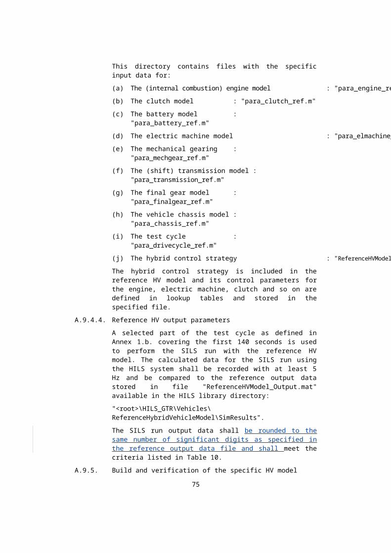
Table 14 Electrical Auxiliaryauxiliary model parameters and interface

T Name Unit Description Reference

Pa Pel,aux W Auxiliary dat.auxiliaryload.-value

Co xP 0-1 Control Aux_flgOnOff_Bp-wrE-lecReq_W

Se iaux A Auxiliary Aux_iAct_A

El u V Voltage phys_voltage_V

El iaux A Current phys_current_A

A.9.7.2.2. Mechanical Auxiliary model

The mechanical auxiliary system shall be modelled using a controllable power loss, Pmech,aux. The power loss shall be implemented as a torque loss act-ing on the representative shaft.

M mech, aux=Pmech, aux/ω (127)

Where:

Pmech,aux :is the mechanical auxiliary power demand (, W)

x : on/off/duty-cycle signal to control auxiliary load level (-)

ω :is the shaft rotational speed (, min-1)

Mmech,aux :is the auxiliary torque (, Nm)

An auxiliary inertia load Jaux shall be part of the model and affect the power-train inertia.

For the model as available in the standardized HILS library, the model parameter and inter-facing definition is given in Table 15.

Table 15Mechanical Auxiliaryauxiliary model parameters and interface

Type / Bus Name Unit Description Reference

Parameter Pmech,aux W Auxiliary system load dat.auxiliaryload.valueParameter Jaux kgm2 Inertia Dat.inertia.value

Command signal xPmech,aux 0-1W Control signal for aux-iliary system power de-mand

Aux_flgOnOff_BpwrMechReq_W

Sensor signal MoutMaux Nm Auxiliary system torque output

Aux_tqAct_A

75

Mech inout [Nm]

MoutMaux Nm Torque phys_torque_Nm

JoutJaux kgm2 Inertia phys_inertia_kgm2

Mech fb outin [rad/s]

ω rad/s speedSpeed phys_speed_radps

Table XXXMechanical auxiliary model parameters

Parameter Parameter type Reference paragraph

Jaux Manufacturer specified -

A.9.7.3. Chassis model

A basic model of the chassis (the vehicle) shall be represented as an inertia. The model shall compute the vehicle speed from a propeller shaft torque and brake torque. The model shall include rolling and aerodynamic drag resist-ances and take into account the road slope resistance. A schematic diagram is shown in Figure 24.

Figure 2425Chassis (vehicle) model diagram

The basic principle shall be input torque Min to a gear reduction (final drive gear) with fixed ratio rfg.

The drive torque Mdrive shall be counteracted by the friction brake torque Mbrake. The result-ingMfric_brake. The brake torque actuator shall be modelled as a first order sys-tem as follows:

M fricbrake=−1

τ1( M fricbrake

−M fricbrake , des ) (XXX)

76

Where:

Mfric_brake is the friction brake torque shall be converted to, Nm

Mfric_brake,des is the drive force usingdesired friction brake torque, Nm

τ1 is the wheel radius rwheel in accordance with equation 129 and acts on the road to drive the vehicle: friction brake actuator time response constant

(Eq. 129)

The force Fdrivetotal drive torque shall balance with forcestorques for aerody-namic drag FaeroMaero, rolling resistance FrollMroll and gravitation FgravMgrav to find resulting acceleration force according torque in accordance with differ-ential equation 130:

J tot ωwheel=M drive−M fricbrake−M aero−M roll−M grav (130)

Where:

mtot : Jtot is the total massinertia of the vehicle (kg), kgm2

❑❑ is the wheel rotational acceleration (m, rad/s)

The total massinertia of the vehicle mtotJtot shall be calculated using the vehicle mass mvehicle and the inertia load from the powertrain components:

J tot=mvehicle ×rfg2 +J powertrain+J wheel (131)

Where:

mvehicle : Massis the mass of the vehicle (, kg)

Jfg : Inertia of the final gear (kgm2)

Jpowertrain : Sumis the sum of all powertrain inertias (, kgm2)

Jwheel : Inertiais the inertia of the wheels (, kg/m2)

The wheelvehicle speed vvehicle shall be determined from the vehiclewheel speed ωwheel and wheel radius rwheel as:

vvehicle=ωwheel ×rwheel (132)

The aerodynamic drag forcetorque shall be calculated as:

M aero=0.5 × ρa ×Cdrag × A front × v vehicle2 ×rwheel (133)

Where:

Ρair :ρa is the air density (, kg/m3)

Cdrag :is the air drag coefficient (-)

Afront :is the total vehicle frontal area (, m2)

vvehicle : is the vehicle speed (, m/s)

The rolling resistance and gravitational torque shall be calculated usingas fol-lows:

(Eq. 134)

M roll=f roll× mvehicle × g×cos (α road)× rwheel (134)

77

M grav=mvehicle × g ×sin (α road)× rwheel (XXX)

Where:

froll :is the friction factor for wheel-road contact (-)

g :is the standard earth gravitation (, m/s2)

α : αroad is the road slope (, rad

The positive hybrid system work shall be determined in the chassis model as:

W sys=∫0

T

max ¿¿ (134)


Table 16Chassis model parameters and interface


Parameter mvehicle kg Vehicle mass dat.vehicle.mass.value

rfg - Final gear ratio dat.fg.ratio.value

ηfg - Final gear efficiency dat.fg.efficiency.value

Jfg kgm2 Final gear inertia dat.fg.inertia.value

Afront m2 Vehicle frontal area dat.aero.af.value

CdCdrag - Air drag coefficient dat.aero.cd.value

rwheel m Wheel radius dat.wheel.radius.value

Jwheel kgm2 Wheel inertia dat.wheel.inertia.value

ffroll - Rolling resistance coefficient

dat.wheel.rollingres.value

τ1 Brake actuator time constant

dat.brakeactuator.timecon-stant.value

Command sig-nal

Mbrake Nm Requested brake torque

Chassis-chassis_tqBrakeReq_Nm

Sensor signal vvehicle m/s Actual vehicle speed Chassischassis_vVehAct_mps

ωwheel rad/s Actual wheel speed Chassis-chassis_nWheelAct_radps

mtot kg Vehicle mass Chassis-chassis_massVehAct_kg

Mdrive Nm Actual wheel hub torque

chassis_tqSysAct_Nm

78

ααroad rad Road slope Chassischassis_slopRoad_rad

Mech in [Nm] Mdrive Nm torqueTorque phys_torque_Nm

Jpowertrain kgm2 inertiaInertia phys_inertia_kgm2

Mech fb out [rad/s]

ωwheel rad/s Rotational speed phys_speed_radps

Table XXXChassis model parameters


mvehicle Regulated A.9.5.6.X., A.9.6.2.X., A.10.X.X.Afront Regulated A.9.5.6.X., A.9.6.2.X., A.10.X.X.

Cdrag Regulated A.9.5.6.X., A.9.6.2.X., A.10.X.X.rwheel Regulated A.9.5.6.X., A.9.6.2.X., A.10.X.X.

Jwheel Regulated A.9.5.6.X., A.9.6.2.X., A.10.X.X.froll Regulated A.9.5.6.X., A.9.6.2.X., A.10.X.X.

τ1 Tuneable default: 0.1 second

A.9.7.4. Driver modelmodels

The driver model shall actuate the accelerator and brake pedal signals to real-ize the desired vehicle speed cycle and apply the shift control for manual transmissions through clutch and gear control. Three different models are available in the standardized HILS library.

Figure 25A.9.7.4.1 Driver output of recorded data

Recorded driver output data from actual powertrain tests may be used to run the vehicle model diagram in open loop mode. The driver model was prepared by following a modular approach data for the ac-celerator pedal, the brake pedal and therefore contains different sub-modules. The model shown in Figure 25 is capable of running a vehicle equipped , in case a vehicle with either a manual gearbox with accelerator, brake and clutch pedal signals or a vehicle equipped with an automated gearbox where only accelerator and brake pedal are used. For the manual shift transmission vehicle the decisions for gear shift manoeuvres are taken by the gear selector submodule. For auto-mated gearboxes this is bypassed but can be enabled also if needed.

The presented driver model contains following:

(a) Sub-module controlling the vehicle speed (PID controller);

(b) Sub-module taking decisions of gear change;

(c) Sub-module actuatingis represented, the clutch pedal;

79

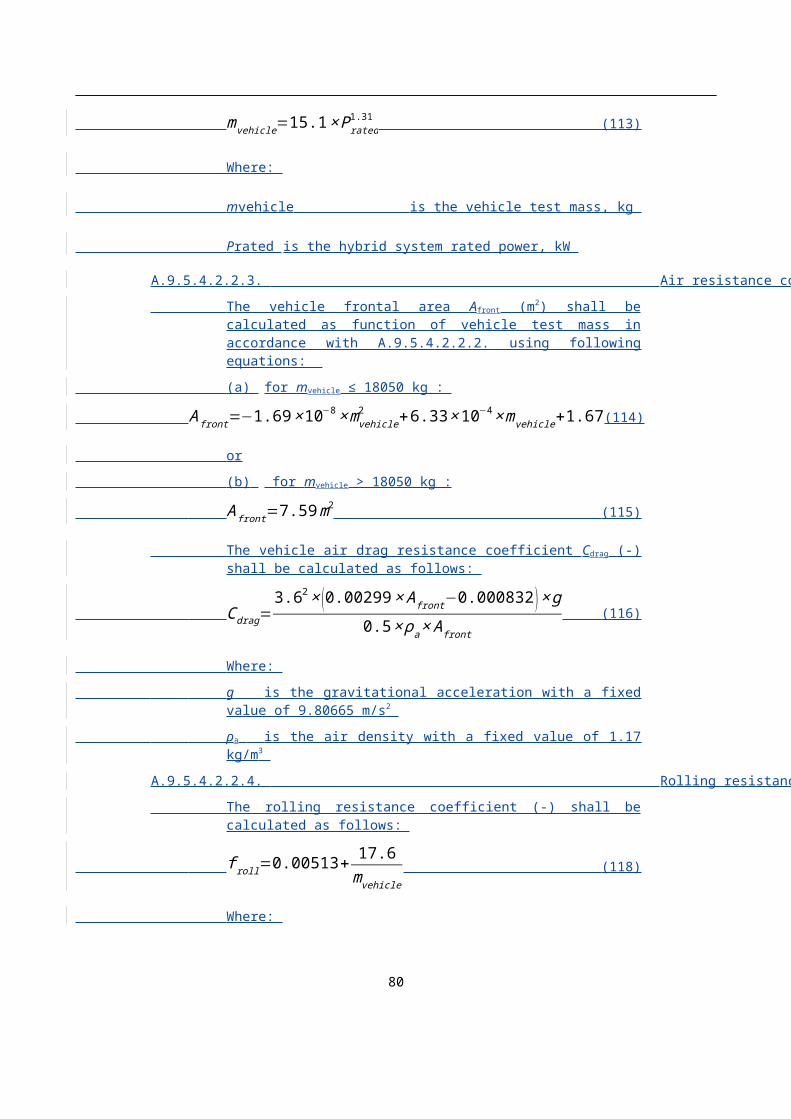
(d) Sub-module switching signals when either a manual or an automated gearbox is used.

For specific demands, the individual sub-modules (as listed above) can and gear position shall therefore be easily removed or be copied to manufacturer specific driver models.

Details for the submodules (a) through (d) are given below:

(a) The sub-module controlling the vehicle speed is modelled using a simple PID-controller. It takes the reference speed from the driving cycle and compares it to the vehicles actual speed. If the vehicle’s speed is to low it uses the accelerator pedal to demand acceleration, and vice versa if the vehicle’s speed is too high, the driver uses the brake pedal to demand a deceleration of the vehicle. For vehicles not capable of running the desired speed (e.g. their design speed is lower than the demanded speed during the test run) the controller includes an anti-wind up provided in a dataset as a function of the integral part, which can be also parameterized in the parameter file. If vehicles equipped with a manual transmission gearbox are driven it is con-sidered that the accelerator pedal is not actuated during a gearshift manoeuvre.

(b) The implemented gearshift strategy is based on the definition of shift polygons for up- and downshift manoeuvres. Together with a full load torque curve and a negative torque curve they describe the permitted operating range of the system. Crossing the upper shift polygon forces selection of a higher gear, crossing the lower one the selection of a lower gear (see Figure 26 below).

The input signals needed for the gear selector sub-module to derive an actual gear request currently are:

- The actual gear engaged;

- The input torque and rotational input speed for the transmis-sion;

- Status of the drivetrain (next gear engaged and all clutches closed and synchronized again).

Figure 26:

Gear shift model using polygons

Internally, also the test cycle and the time of clutch actuation during a shift manoeuvre are loaded in order to detect vehicle starts form stand-still and engage the 1st gear on time before the desired speed is greater zero. This allows the vehicle to follow the desired speed within the given limits. The standard output value of the gearshift module when the vehicle stands still is the neutral gear. After a gear is changed a subsequent gear change is suppressed for a parameterized time and as long as the drivetrain is not connected to all propulsion engines and not fully synchronized again. The time limit is rejected and a next gear change is forced if rotational speed limits (lower than ICE idle speed or greater than ICE rated speed multiplied by 1.2) are exceeded.

80

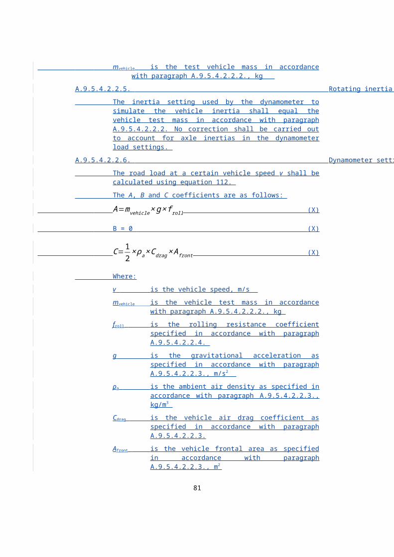
(c) The sub-module actuating the clutch pedal was designed to actuate the pedal if a vehicle equipped with a manual transmission gearbox is used. Excluding the function from the speed controller sub-module en-ables the driver model to be used in a wider field of applications. The clutch sub-module is triggered by the gear selector module and actu-ates the pedal as soon as a gearshift manoeuvre is requested. The clutch module simultaneously forces the speed controller to put the ac-celerator pedal to zero as long as the clutch is not closed and fully syn-chronized again after the gearshift manoeuvre. The time of clutch ac-tuation has to be specified in the driver parameter file.

(d) The AT/MT switch enables the driver model to be used either for a vehicle with a manual or an automated gearbox. The output signals for the MT mode are the requested gear and the accelerator-, brake-, and clutch pedal ratios. Using the AT mode the output signals are only ac-celerator- and brake pedal ratio. No gearshift manoeuvres are con-sidered and therefore the accelerator pedal is also not set to zero even though a gear change is detected. The standard values for the clutch pedal ration and for a desired gear are zero in AT mode. Nevertheless, if the gear selection of the actual test vehicle should be overruled this can be done by enabling the desired gear output in the parameter file.

. For the model as available in the standardized HILS library, the model para-meter and interfacing definition is given in Table 17X.

Table 17 XDriver model parameters and interface


Parameter - Select gearbox mode MT(1) or AT(0)

dat.gearboxmode.value

- Gear selection model dat.gearselectionmode.value

s Clutch time dat.clutchtime.value

m/s Clutch is automatically acutated when speed is below this value

dat.clutchthershold.value

- Driver PID controller dat.controller

Command sig-nal

pedalbrake 0-1 AcceleratorRequested brake pedal position

Drv_AccPedl_ratBrkPedl_Rt

pedalaccelerator 0-1 BrakeRequested acceler-ator pedal position

Drv_BrkPedl_ratAccPedl_Rt

pedalclutch 0-1 ClutchRequested clutch pedal position

Drv_CluPedl_ratRt

- - Gear request Drv_nrGearReq

m/s Reference target speed Drivecycle_RefSpeed_mps

Sensor signal - m/s- Chassis speed- Chassis_vVehAct_mps-

81

rad/s Transmission input speed

Transm_nInAct_radps

Nm Transmission input torque

Transm_tqInAct_Nm

- Actual gear ratio Transm_grGearAct

Boolean Transmission status Transm_flgConnected_B

Boolean Clutch status Clu_flgConnected_B

A.9.7.4.2 Driver model for vehicles without a shift transmission or equipped with auto-matic or automated manual transmissions

The driver model is represented by a commonly known PID-controller. The model output is depending on the difference between the reference target speed from the test cycle and the actual vehicle speed feedback. For vehicle speeds below the desired speed the accelerator pedal is actuated to reduce the deviation, for vehicle speeds greater than the desired speed the brake pedal is actuated. An anti-windup function is included for vehicles not capable of run-ning the desired speed (e.g. their design speed is lower than the demanded speed) to prevent the integrator windup. When the reference speed is zero the model always applies the brake pedal to prevent moving of the vehicle due to gravitational loads. For the model as available in the standardized HILS lib-rary, the model parameter and interfacing definition is given in Table X.

Table XDriver model parameters and interface


Parameter KP

KI

KD

-

-

-

PID controller para-meters

dat.controller.p.value

dat.controller.i.value

dat.controller.d.value

KK - Anti-windup term dat.controller.k.value

Command signal

pedalbrake 0-1 Requested brake pedal position

Drv_BrkPedl_Rt

pedalaccelerator 0-1 Requested acceler-ator pedal position

Drv_AccPedl_Rt

- m/s Reference target speed

Drivecycle_RefSpeed_mps

Sensor signal vvehicle m/s Actual vehicle speed Chassis_vVehAct_mps

Table XXXDriver model parameters


82

KP, KI, KD Tuneable -

KK Tuneable -

A.9.7.4.3 Driver model for vehicles equipped with manual transmission

The driver model consist of a PID-controller as described in A.9.7.4.2, a clutch actuation module and a gearshift logic as described in A.9.7.4.3.1. The gear shift logics module requests a gear change depending on the actual vehicle running condition. This induces a release of the accelerator pedal and simultaneously actuates the clutch pedal. The accelerator pedal is fully re-leased until the drivetrain is synchronized in the next gear, but at least for the specified clutch time. Clutch pedal actuation of the driver (opening and clos-ing) is modelled using a first order transfer function. For starting from stand-still, a linear clutch behaviour is realized and can be parameterized separately (see Figure X).

Figure 26Clutch pedal operation (example)

For the model as available in the standardized HILS library, the model para-meter and interfacing definition is given in Table X.

Table XDriver model parameters and interface


Parameter KP

KI

KD

-

-

-

PID controller para-meters


dat.controller.i.value

dat.controller.d.value

KK - Anti-windup term dat.controller.k.value

Tclutch s Specified clutch time

dat.clutchtime.value

τopen s Opening time con- dat.clutchtime.open.value

83

stant

τclose s Closing time con-stant

dat.clutchtime.close.value

Tdriveaway s Closing time at drive away

dat.clutchtime.driveaway.-value

Command signal

pedalbrake 0-1 Requested brake pedal position

Drv_BrkPedl_Rt

pedalaccelerator 0-1 Requested acceler-ator pedal position

Drv_AccPedl_Rt

- m/s Reference target speed

Drivecycle_RefSpeed_mps

- - Gear request Drv_nrGearReq

pedalclutch 0-1 Requested clutch pedal position

Drv_CluPedl_Rt


ωin rad/s Transmission input speed

Transm_nInAct_radps

- - Actual gear engaged Transm_nrGearAct

- Boolean Clutch disengaged or not

Clu_flgConnected_B

Table XXXDriver model parameters


KP, KI, KD Tuneable -

KK Tuneable -

Tclutch Regulated A.9.6.2.15.τopen Tuneable Default: 0.01

τclose Tuneable Default: 0.02Tdriveaway Tuneable Default: 2

A.9.7.4.3.1 Gear shift strategy for manual transmissions

The gear shift strategy for a (manual) shift transmission is available as a sep-arate component module and therefore can be integrated in other driver mod-els different from the one as described in paragraph A.9.7.4.3. Besides the specified parameters below, the gear shift strategy also depends on vehicle and driver parameters which have to be set in the parameter file according to the respective component data as specified in Table X.

84

The implemented gearshift strategy is based on the definition of shifting thresholds as function of engine speed and torque for up- and down shift manoeuvres. Together with a full load torque curve and a friction torque curve, they describe the permitted operating range of the system. Crossing the upper shifting limit forces selection of a higher gear, crossing the lower one will request the selection of a lower gear (see Figure 27 below).

Figure 27Gear shift logic (example)

The values for the shifting thresholds specified in Table X shall be calculated based on the data of the internal combustion engine full load torque curve and friction torque curve (as obtained in accordance with paragraph A.9.8.3.) as follows:

(a) The characteristic points P1 to P6 in Figure X are defined by the coordinate pairs listed in Table X.

(b) The slope k1 of the line between P1 and P3 as well as the slope k2 of the line between P2 and P4 are calculated as follows:

k1=y3− y1

x3−x1 (XXX)

85

k 2=y 4− y2

x4−x2 (XXX)

(c) The downshift limits speed vector shall consist of the three values: [x5, x5, x3]

(d) The downshift limits torque vector shall consist of the three values:

[y5, k1 ×(x5−nidle

2), y3]

(e) The upshift limits speed vector shall consist of the three values:

[x6, x6, x4]

(f) The upshift limits torque vector shall consist of the three values:

[y6, k 2×(x6−nidle ), y4].

Table XXXShift logic coordinate pairs

Point x-coordinate(engine speed, min-1 )

y-coordinate(engine torque, Nm)

P1 ❑❑❑❑

❑y1 = 0

P2 ❑❑❑❑ y2 = 0

P3 ❑❑❑❑❑❑

❑y3 = Tmax

P4 ❑❑❑❑ y4 = Tmax

P5 ❑❑❑❑❑❑ y5 = Tmin

P6 ❑❑❑❑❑❑ y6 = Tmin

Where in the above:

Tmax is the overall maximum positive engine torque, Nm

Tmin is the overall minimum negative engine torque, Nm

nidle, nlo, npref, n95h are the reference speeds as defined in accordance with paragraph 7.4.6., min-1

Also the driving cycle and the time of clutch actuation during a shift man-oeuvre (Tclutch) are loaded in order to detect vehicle starts from standstill and engage the start gear in time (Tstartgear) before the reference driving cycle speed changes from zero speed to a value above zero. This allows the vehicle to fol-low the desired speed within the given limits.

The standard output value of the gearshift module when the vehicle is at stand still is the neutral gear.

86

After a gear change is requested, a subsequent gear change request is sup-pressed for a period of 3 seconds and as long as the drivetrain is not connec-ted to all propulsion machines and not fully synchronized again (Dtsyncindi). These limiting conditions are rejected and a next gear change is forced when certain defined limits for the gearbox input speed (lower than ICE idle speed or higher than ICE normalized speed of 1.2 (i.e. 1.2 x (rated speed – idle speed) + idle speed)) are exceeded.

After a gear change is finished, the friction clutch actuated by the driver has to be fully connected again. This is particularly important during decelera-tions of the vehicle. If a deceleration occurs from a certain speed down to standstill, the friction clutch actuated by the driver has to be connected again after each downshift. Otherwise, the gear shift algorithm will not work prop-erly and the simulation will result in an internal error. If shifting down one gear after the other (until the neutral gear is selected) during braking with very high decelerations shall be avoided, the friction clutch actuated by the driver has to be fully disconnected during the entire deceleration until the vehicle is standing still. Once the vehicle speed is zero the neutral gear will be selected and the friction clutch actuated by the driver can be connected again allowing the vehicle to start from standstill as soon as the driving cycle demands so.

If the accelerator pedal is fully pressed, the upper shifting limit is not in force. In this case, the upshift is triggered when the gearbox input speed gets higher than the ICE rated speed (i.e. when the point of maximum power is exceeded).

A skip gear function for upshifting can be enabled (SGflg) for transmissions with a high number of gears to avoid unrealistic, too frequent shift behaviour. In this case, the highest gear for which the gearbox input speed is located above the downshift limit and below the upshift limit for the actual operation point is selected.

Automatic start gear detection is also available (ASGflg) for transmissions with a high number of gears to avoid unrealistic, too frequent shift behaviour. If activated, the highest gear for which the gearbox input speed is above ICE idle speed when the vehicle is driving at 2 m/s and for which a vehicle accel-eration of 1.6 m/s² can be achieved is selected for starting from standstill. If deactivated, starting from standstill is performed in the first (1st ) gear.

The flag signal Dtsyncindi is used as an indicator for a fully synchronized and connected drivetrain. It is involved in triggering upcoming gear shift events. It has to be ensured that this signal becomes active only if the entire driv-etrain runs on fully synchronized speeds. Otherwise the gear shift algorithm will not work properly and the simulation will result in an internal error.

For a correct engagement of the starting gear, the actual vehicle speed has to be zero (no rolling of the vehicle, application of brake necessary). Otherwise a time delay can occur until the starting gear is engaged.

For the model as available in the standardized HILS library, the model para-meter and interfacing definition is given in Table X, where “satp” is used for “set according to respective parameter file and provisions of”. Additional ex-planations are listed below the table for all descriptions marked with an aster-isk (*).

87

Table XGear shift strategy parameters and interface


Parameter Tclutch s satp driver dat.vecto.clutchtime.value

- kg satp chassis dat.vecto.vehicle.mass.value

- m satp chassis dat.vecto.wheel.radius.value

- kgm2 satp chassis dat.vecto.wheel.inertia.value

- - satp chassis dat.vecto.wheel.rollingres.-value

- m2 satp chassis dat.vecto.aero.af.value

- - satp chassis dat.vecto.aero.cd.value

- - satp final gear dat.vecto.fg.ratio.value

- - satp transmission dat.vecto.gear.number.vec

- - satp transmission dat.vecto.gear.ratio.vec

- - satp transmission *1 dat.vecto.gear.efficiency.vec

- rad/s satp engine *2 dat.vecto.ICE.maxtorque_speed.vec

- Nm satp engine dat.vecto.ICE.maxtorque_torque.vec

- Nm satp engine *3 dat.vecto.ICE.maxtorque_friction.vec

- rad/s satp engine *4 dat.vecto.ICE.ratedspeed.-value

- rad/s downshift limits speed vector

dat.vecto.downshift_speed.vec

- Nm downshift limits torque vector

dat.vecto.downshift_torque.vec

- rad/s upshift limits speed vector

dat.vecto.upshift_speed.vec

- Nm upshift limits torque vector

dat.vecto.upshift_torque.vec

SGflg Boolean skip gears when up-shifting active or not

Default: 0

dat.vecto.skipgears.value

Tstartgear s engage startgear dat.vecto.startgearengaged.-

88

prior driveaway value

ASGflg Boolean automatic start gear detection active or not

Default: 0

dat.vecto.startgearactive.-value

Command signal

- - Requested gear nrGearReq


ωin rad/s Transmission input speed

Transm_nInAct_radps

- - Actual gear engaged Transm_nrGearAct

Dtsyncindi Boolean Clutch disengaged or not and drivetrain synchronized or not

Clu_flgConnected_B

- Actual position of accelerator pedal

Drv_AccPedl_rat

*1 The efficiencies of each gear of the transmission do not require a map, but only a single value for each gear since constant efficiencies are defined for the creation of the HEC cycle (in accordance with paragraph A.9.6.2.11.). The gear shift logics for manual transmissions must not be used for model verification (in accordance with paragraph A.9.5.6.14.). and thus do not re-quire an efficiency map for each gear since in this case the gear shifting beha-viour from the actual powertrain test is fed into the model.

*2 The vector of engine speed setpoints defining the full load and friction torque curve has to start with engine idle speed. Otherwise the gear shift algorithm will not work properly.

*3 The vector defining the engine friction torque curve has to consist of values of negative torque (in accordance with paragraph A.9.7.3.).

*4 The engine rated speed value used for parameterizing the gear shift logics for manual transmissions shall be the highest engine speed where maximum power is available. Otherwise the gear shift algorithm will not work properly.

A.9.7.5. Electrical component models

A.9.7.5.1. DCDC converter model

The DC/DC converter is a device that changes the voltage level to the desired voltage level. The converter model is general and captures the behaviour of several different converters such as buck, boost and buck-boost converters. As DC/DC converters are dynamically fast compared to other dynamics in a powertrain a simple static model shall be used:

89

(Eq. ❑❑❑❑❑❑ (135)

Where:

uin :is the input voltage level (, V)

uout :is the output voltage level (, V)

xDCDC :is the conversion ratio, i.e. control signal (-)

The conversion ratio xDCDC shall be determined by an open-loop controller to the desired voltage ureq as:

(Eq. ❑❑❑❑/❑❑ (136)

The DC/DC converter losses shall be defined as current loss using a constant DC/DC converteran efficiency as followsmap in accordance with:

(Eq. 137)

i¿=xDCDC ×iout ×ηDCDC (u¿ , i¿ ) (137)

Where:

ηDCDC :is the DC/DC converter efficiency (-)

iin :is the input current to the DC/DC converter (, A)

iDCDCloss : iout is the output current from the DC/DC converter current loss (, A)


Table 18DC/DC converter model parameters and interface


Parameter ηDCDC - efficiencyEfficiency dat.elecefficiency.efficiency.valuemapCommand signal

ureq V Requested output voltage

dcdc_uReq_V

Sensor signal uout V Actual output voltage

dcdc_uAct_V

Elec in [V] uin V voltageVoltage phys_voltage_V

Elec out [V] uout V voltageVoltage phys_voltage_VElec fb in [A] iout A currentCurrent phys_current_A

Elec fb out [A]

iin A currentCurrent phys_current_A

Table XXXDC/DC converter model parameters


ηDCDC Manufacturer specified -

90

A.9.7.6. Energy converter models

A.9.7.6.1. Electric machine system model

An electric machine can generally be divided into three parts, the stator, rotor and the (high power) electronic controller electronics. The rotor is the rotat-ing part of the machine. The electric machine shall be modelled using maps to represent the relation between its mechanical and electrical (DC) power, see Figure 2728.

Figure 2728:

Electric machine model diagram

The electric machine dynamics shall be modelled as a first order system

M em=−1τ1

× ( M em−M em,des ) (138)

Where:

Mem : Electricis the electric machine torque (, Nm)

Mem,des : Desiredis the desired electric machine torque (, Nm)

τ1 : Electricis the electric machine time response constant (-)

The electric machine system power Pel,em shall be mapped as function of the electric motor speed ωem and, its torque Mem. and DC-bus voltage level u. Two separate maps shall be defined for the positive and negative torquestorque ranges, respectively.

(Eq. Pel , em=f ( M em , ωem ,u ) (139)

The efficiency of the electric machine system shall be calculated as:

91

ηem=M em ×ωem

Pel , em (140)

The electric machine system current iem shall be calculated as:

iem=Pel ,em

u (141)

Where:

iem : electric machine system current (A)

u : battery voltage (V)

Based on its power loss Ploss,em, the electric machine model shall haveprovides a simple thermodynamics model that may be used to derive its temperature Tem as follows:

(Eq. 143)

Ploss, em=P el ,em−M em ×ωem (142)

T em=1

τ em,heat× (P loss ,em−(T em−T em ,cool )/ Rem ,th ) (143)

Where:

Tem : Electricis the electric machine system temperature (, K)

τem,heat : Time constantis the thermal capacity for electric machine thermal mass (), J/K

Tem,cool : Electricis the electric machine system cooling medium temperat-ure (, K)

Rem,th : Electric machine systemis the thermal resistance ()between electric machine and cooling fluid, K/W

The electric machine system shall be torque or speed controlled using, re-spectively, an open-loop (feed-forward) controlcontroller or PI-controller. as follows:

M em, des=K P× (ωref−ωem )+K I ×∫ (ωref−ωem) dt (XXX)

Where:

KP is the proportional gain of speed controller

KI is the integral gain of speed controller

The electric machine torque shall be limited as follows:

M min(ωem)≤ M em ,des ≤ M max (ωem) (XXX)

Where:

Mmin, Mmax are the minimum and maximum torque maps as function of the rotational speed.

The electric machine model shall also include an inertia load Jem that shall be added to the total powertrain inertia.

92


Table 19: Electric machine model parameters and interface


Parameter Jem kgm2 Inertia dat.inertia.value

τ1 - Time constant dat.timeconstant.value

Mmax Nm Maximum torque =f(speed)

dat.maxtorque.torque.vec

Mmin Nm Minimum torque =f(speed)

dat.mintorque.torque.vec

KP

KI

-

-

Speed controller (PI) dat.ctrlcontroller.p.value


Pel,em W Power map =f(speed,torque,voltage)

dat.elecpowmap.motor.elecpowmap

dat.elecpowmap.genertor.elecpowmap

kg/s mass flow cooling fluid dat.mflFluid

Optional parameters

τem,heat J/K Thermal capacity dat.cm.value

Rth K/W Thermal resistance dat.Rth.value

- - Properties of the cooling fluid

dat.coolingFluid

Command signal

ωref rad/s Requested speed ElecMac_nReq_radps

- boolean Switch speed/torque control

ElecMac_flgReqSwitch_B

Mem,des Nm Requested torque ElecMac_tqReq_Nm

Sensor sig-nal

Mem Nm Actual machine torque ElecMac_tqAct_Nm

ωem rad/s Actual machine speed ElecMac_nAct_radps

i A Current ElecMac_iAct_A

Tem K Machine temperature ElecMac_tAct_K

Elec in [V] u V voltage phys_voltage_V

Elec fb out [A]

i A current phys_current_A

Mech out Mem Nm torque phys_torque_Nm

93


[Nm]

Jem kgm2 inertia phys_inertia_kgm2

Mech fb in [rad/s]

ωem rad/s rotational speed phys_speed_radps

Table XXXElectric machine model parameters


Jem Manufacturer specified -τ1 Tunable -

Mmax Regulated A.9.8.4.Mmin Regulated A.9.8.4.

KP, KI TunablePel,em Regulated A.9.8.4.

A.9.7.6.2. Hydraulic pump/motor model

A hydraulic pump/motor generally converts energy stored in a hydraulic ac-cumulator to mechanical energy as schematically shown in Figure 29.

Figure 29:

Hydraulic pump/motor model diagram

The pump/motor torque shall be modelled as:

M pm=x× D pm× ( pacc−pres )× ηpm❑

(144)

Where:

94

Mpm :is the pump/motor torque (, Nm)

x :is the pump/motor control command signal between 0 and 1 (-)

D :Dpm is the pump/motor displacement (, m3)

pacc :is the pressure in high pressure accumulator (, Pa)

pres :is the pressure in low pressure sump/reservoir (, Pa)

ηpm :is the mechanical pump/motor efficiency (-)

The mechanical efficiency ηpm shall be determined using:

(Eq. 145)

And be calculatedfrom measurements and mapped as function of friction losses, hydrodynamic losses and viscous lossesthe control command signal x, the pressure difference over the pump/motor and its speed as follows:

(Eq. 146)

ηpm=f ( x , pacc , pres ,ωpm ) (145)

Where:

ωpm :is the pump/motor speed (rad/s)

The efficiency can be determined from experimental data.

The volumetric flow Qpm through the pump/motor shall be calculated as:

(Eq. 148)

Q pm=x × D pm× ωpm ×ηvpm❑ (147)

The volumetric efficiency mayshall be determined from measurements and mapped as function of the control command signal x, the pressure difference ofover the pump/motor and its speed as follows:

(Eq. 149)

ηvpm= f ( x , pacc , pres ,ω pm ) (149)

The hydraulic pump/motor dynamics shall be modelled as a first order system in accord-ance with:

x pm=−1τ1

× ( x pm−u pm, des ) (138)

Where:

xpm is the output pump/motor torque or volume flow, Nm or m3 /s

upm,des is the input pump/motor torque or volume flow, Nm or m3 /s

τ1 is the pump/motor time response constant

The pump/motor system shall be torque or speed controlled using, respectively, an open-loop (feed-forward) control or PI-controller. as follows:

M pm,des=KP × ( ωref−ωpm )+K I ×∫ (ωref−ωpm ) dt (XXX)

Where:

95



The hydraulic pump/motor torque shall be limited as follows:

M pm ,des ≤ M max (ω pm) (XXX)

Where:

Mmax is the and maximum torque map as function of the rotational speed.

The hydraulic pump/motor model shall also include an inertia load Jpm that shall be added to the total powertrain inertia.


96

Table 20Hydraulic Pump/Motor model parameters and interface


Parameter Jpm kgm2 Inertia dat.inertia.value

τ1 - Time constant dat.timeconstant.value

Mmax Nm Maximum torque =f(speed)

dat.maxtorque

D m3 Displacement volume

dat.displacement.value

ηv - Volumetric effi-ciency

dat.volefficiency.efficiency.map

ηm - Mechanical effi-ciency

dat.mechefficiency.efficiency.map

KP

KI

--

PI controller dat.ctrlcontroller.p.valuedat.controller.i.value

Command sig-nal

ωref rad/s Requested speed Hpm_nReq_radps

- boolean Switch speed/torque control

Hpm_flgReqSwitch_B

Mpm,des Nm Requested torque Hpm_tqReq_Nm

Sensor signal MemMpm Nm Actual machine torque

Hpm_tqAct_Nm

ωpm rad/s Actual machine speed

Hpm_nAct_radps

Qpm m3/s Actual volumet-ric flow

Hpm_flowAct_m3ps

pacc Pa Accumulator pressure

Hpm_pInAct_Pa

pres Pa Reservoir pres-sure

Hpm_pOutAct_Pa

Fluid in 1 [Pa] pacc Pa pressure phys_pressure_Pa

Fluid in 2 [Pa] Pres Pa pressure phys_pressure_Pa

Fluid out [m3/s]

Qpm m3/s Volume flow phys_flow_m3ps

Mech out [Nm]

Mpm Nm torque phys_torque_Nm

Jpm kgm2 inertia phys_inertia_kgm2

Mech fb in [rad/s]

ωpm rad/s rotational speed phys_speed_radps

97

Table XXXHydraulic pump/motor model parameters


Jpm Manufacturer specified -

τ1 Manufacturer specified -Mmax Manufacturer specified -

D Manufacturer specified -ηv Manufacturer specified -

ηm Manufacturer specified -KP, KI Tuneable -

A.9.7.6.3. Internal Combustion Engine model

The internal combustion engine model shall be modelled using maps to rep-resent the chemical to mechanical energy conversion and the applicable time response. for torque build up. The internal combustion engine model diagram is shown in Figure 2829.

Figure 2829

Internal combustion engine model diagram

The internal combustion engine shall include engine friction and exhaust braking, both as function of engine speed and modelled using maps. The ex-haust brake can be controlled using e.g. an on/off control command signal. or continuous signal between 0 and 1. The model shall also include a starter motor, modelled using a constant torque Mstart. The internal combustion en-gine shall be started and stopped by a control signal.

The torque build-up response model shall use either of the following meth-ods:

(a) Using abe modelled using two first -order model with fixed time con-stant (version 1)models. The first shall account for almost direct torque build-up representing the fast dynamics as follows:

98

(Eq. 150)

❑❑❑❑❑

(❑❑❑❑❑❑) (150)

Where:

Mice : ICE,1 is the fast dynamic engine torque (, Nm)

Mice,des : ICEdes1 is the fast dynamic engine torque demand torque (, Nm )

Τice :τice,1 is the time constant for ICEfast engine torque response model (s)

(b) Using a ωice is the engine speed, rad/s

The second first-order model withsystem shall account for the slower dynam-ics corresponding to turbo charger effects and boost pressure build-up as fol-lows:

M ice, 2=−1

τ ice, 2(ωice )× (M ice ,2−M ice, des 2(ωice )) (151)

Where:

Mice,2 is the slow dynamic engine torque, Nm

Mice,des2 is the slow dynamic engine torque demand, Nm

τice,2 is the speed dependent time constant (version 2) as follows:

(Eq. 152)

Where:

Mice : ICE torque (Nm)

Mice1 : dynamic ICE torque (Nm)

Mice,des1 : dynamic ICE demand torque (Nm)

Mice,des2 : direct ICE demand torque (Nm)

τice : speed dependent time constant for ICEfor slow engine torque response model (s)

ωice : engine speed (rad/s)

Both the speed dependent time constant and the dynamic and direct torque di-vision are mapped as function of speed.

The total engine torque Mice shall be calculated as:

M ice=Mice ,1+M ice, 2 (152)

The internal combustion engine model shall haveprovides a thermodynamics model that may be used to represent the engine heat-up from cold start to its normal stabilized operating temperatures in accordance with:

T ice, oil=max (T ice, oil , heatup=f ( Pice, loss ) ,T ice , oil , hot ) (153)

Where:

Tice,oil : is the ICE oil temperature (, K)

Pice,loss : are the ICE power losses (, W)

99

η : fraction of power loss that goes to heating (-)

θice,oil,cold : Since no fuel consumption and efficiency map is avail-able in the model Pice,loss = (ωice x Mice) is used as a simplified approach. Adap-tion of the warm-up behaviour can be made via the function Tice,oil,heatup = f(Pice,loss).

Tice,oil,heatup is the ICE oil temperature at (cold) start (, K)

θiceTice,oil,hot : is the ICE oil temperature at normal warm-up operatingoperation condition (, K)

The internal combustion engine shall be torque or speed controlled using, re-spectively, an open-loop (feed-forward) control or PI-controller. For both controllers the desired engine torque can be either the desired indicated torque or the desired crankshaft torque. This shall be selected by the para-meter Mdes,type. The PI controller shall be in accordance with:

M ice, des=K P× (ωref−ωice )+K I ×∫ (ωref−ωice) dt (XXX)

Where:



The internal combustion engine torque shall be limited as follows:

M ice, des≤ M max(ωice) (XXX)

Where:

Mmax is the and maximum torque map as function of the rotational speed.

The internal combustion engine model shall also include an inertia load Jice that shall be ad-ded to the total powertrain inertia.


Table 21Internal Combustion Engine model parameters and interface

T Na U De- Ref-

P J k Inertia dat.i

τ - Time dat.-

τ - Time dat.

M N En- dat.

M N Ex- dat.

M N Max- dat.

100

T Na U De- Ref-

max m imum torque =f(speed)

maxtorque.t-orque.vec

KP

KI

-

-

PI dat

dat.

k Fuel dat.

M k Net dat

M k Fuel

(0) in-

(1)

dat

- Power dat.

O - Prop- dat.

- Prop- dat.

C ω r Re- Eng

- b Switc Eng

M N Re- Eng

b Ex- Eng

b En- Eng

b Starter Eng

101

T Na U De- Ref-

b Fuel Eng

S M N Crank Eng

M N Indic- Eng

ω r Actual Eng

T K Oil Eng

C k Fuel phys_mass-

M M N torque phy

J k inertia phy

M ω r rota- phy

Table XXXInternal combustion engine model parameters


Jice Manufacturer specified -

τice,1 Regulated A.9.8.3.τice,2 Regulated A.9.8.3.

Mfric Regulated A.9.8.3.Mexh Regulated A.9.8.3.

Mmax Regulated A.9.8.3.KP, KI Tunable -

Mstart Manufacturer specified -Mdes,type Manufacturer specified -

A.9.7.7. Mechanical component models

A.9.7.7.1. Clutch model

102

The clutch model shall transfer the input torque on the primary clutch plate to the secondary clutch plate applyingmoving through three operating phases, i.e. 1) opened, 2) slipping and 3) closed. Figure 29 30 shows the clutch model diagram.

Figure 2930

Clutch model diagram

The clutch model shall be defined in accordance with following (differential) equations of motion:

Jcl ,1× ωcl ,1=M cl 1 ,∈¿−M cl¿ (154)

Jcl ,2× ωcl ,2=M cl−M cl2 ,out (155)

During clutch slip operation following relation is defined:

M cl=ucl × M cl , maxtorque × tanh (c×(ω1−ω2)) (156)

ω1=ω2|t=0+∫0

t

¿¿ (157)

Where:

Mcl,maxtorque :is the maximum transferrable torque transfer through the clutch (, Nm)

ucl :is the clutch actuation control signal between 0 and 1 (-)

c is a tuning constant for the hyperbolic function tanh().

When the speed difference between ω1 – ω2 is below the threshold limit sliplimit and the clutch pedal position is above the threshold limit pedallimit, the clutch shall no longer be slipping and considered to be in closed locked mode.

During clutch open and closed operation, the following relations shall apply:

1) for clutch open (Eq. :

M cl=0 (158)

103

2) for clutch closed (Eq. :

M cl2 , out=M cl1 ,∈¿¿ (159)

The clutch pedal actuator shall be represented as a first order system:

ucl=−1τ1

× (ucl−u pedal) (XXX)

Where:

ucl is the clutch actuator position between 0 and 1

u is the clutch pedal position between 0 and 1

τ1 is the clutch time constant


104

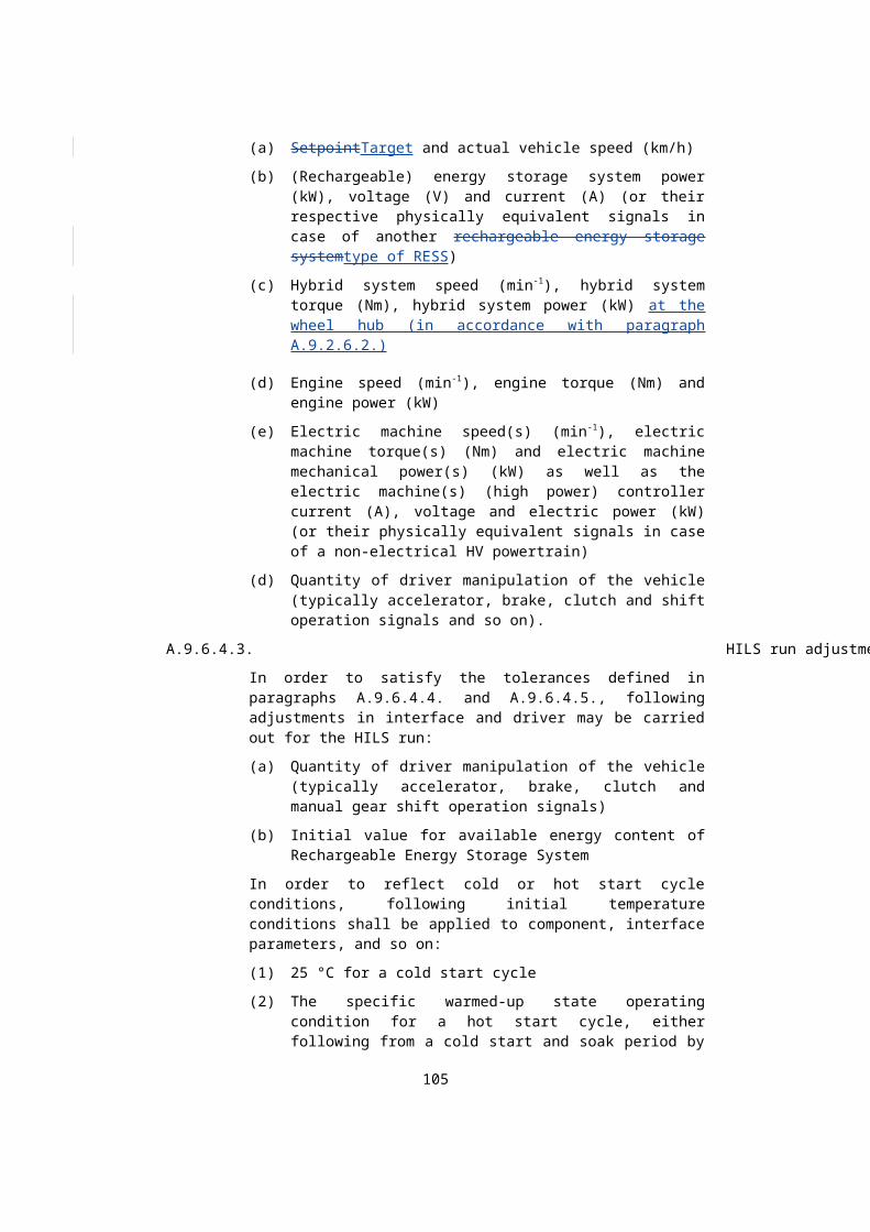
Table 22Clutch model parameters and interface

Type / Bus Name Unit De Reference

P J1 kgm In dat.in.inertia.-value

J2 kgm In dat.out.inertia.-value

Mmax- Nm M dat.maxtorque.-value

c - Tu dat.tanh.value

sli rad/s Sli dat.speedtoler-ance.-value

ped- - Sli dat.clutch-threshold-.-value

τ1 - Ti dat.actuator.-time-con-stant.value

Com- u 0-1 Re Clu_ratReq_Rt

Sensor boole Cl Clu_flgConnec-te

105

d_B

Mech in Min Nm tor phys_torque_Nm

Jin kgm in phys_inertia_kgm2

Mech Mout Nm tor phys_torque_Nm

Jout kgm in phys_inertia_kgm2

Mech fb ω1 rad/s ro phys_speed_radps

Mech fb ω2 rad/s ro phys_speed_radps

Table XXXClutch model parameters


J1 Manufacturer specified A.9.5.6.X.J2 Manufacturer specified A.9.5.6.X.

Mcl,maxtorque Manufacturer specified A.9.5.6.X.c Tuneable default: 0.2

sliplimit Tuneable default: 1pedallimit Tuneable default: 0.8

τ1 Manufacturer specified -

A.9.7.7.2. Continuously Variable Transmission model

The Continuously Variable Transmission (CVT) model shall represent a mechanical transmission that allows any gear ratio between a defined upper and lower limit. The CVT model shall be in accordance with:

(Eq. 160)

M CVT ,out=r CVT MCVT ,∈¿ ηCVT ¿ (160)

Where:

MCVT,in :is the CVT input torque (, Nm)

MCVT,out :is the CVT output torque (, Nm)

rCVT :is the CVT ratio (-)

ηCVT :is the CVT efficiency (-)

106

The CVT efficiency shall be defined as function of input torque, output speed and gear ratio:

(Eq.

ηCVT= f ¿ (161)

The CVT model shall assume zero speed slip, so that following relation for speeds can be used:

(Eq. 162)

ωCVT ,∈¿=rCVT ωCVT ,out ¿ (162)

The gear ratio of the CVT shall be controlled by a command setpoint and us-ing a first-order representation for the CVT ratio change actuation in accord-ance with:

(Eq. 163)

ddt

rCVT=1

τCVT(−rCVT +rCVT ,des ) (163)

Where:

τCVT :is the CVT time constant (, s)

rCVT,des :is the CVT commanded gear ratio (-)


Table 23 CVT model parameters and interface

T Na U De- Reference

P τ - Time dat.timecon-stant.value

η - Effi- dat.mecheffi-cienc

107

y. efficiency.map

M N Max- dat.max-torque.value

C r - Re- CVT_ratGe-arReq

S r - Ac- CVT_rat-GearAct_Rt

ω r Out- CVT_nOutAct_r

108

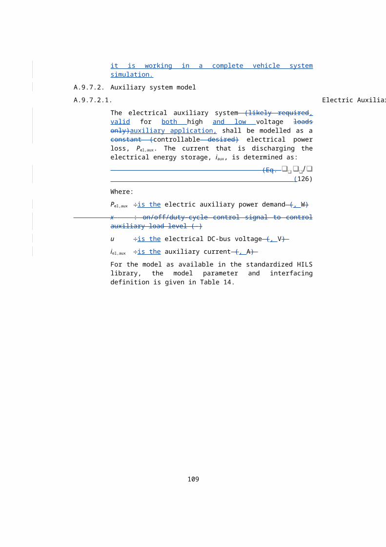
adps

ω r Input CVT_nInAct_radps

M M N torqu phys_torque_Nm

Jin k iner- phys_inertia_kgm2

M M N torqu phys_torque_Nm

J k iner- phys_inertia_kgm2

M ω r rota- phys_speed_radps

M ω r rota- phys_speed_radps

A.9.7.7.3. Flywheel model

The flywheel model shall represent a rotating mass that is used to store and release kinetic energy. The flywheel kinetic energy state is defined by:

(Eq. 165)

Where:

Mflywheel,in : input torque to flywheel (Nm)

Mflywheel,loss : (speed dependent) flywheel losses (Nm)

109

The losses may be determined from measurements and modelled using maps.


Table 24

Flywheel

Table XXXCVT model parameters and interface


τCVT Manufacturer specified

-

ηCVT Manufacturer specified

-

A.9.7.7.3. Final gear model

A final gear transmission with a set of cog wheels and fixed ratio shall be represented in accordance with following equation:

ωfg ,out=ω fg,∈¿ /rfg ¿ (X)

The gear losses shall be considered as torque losses and implemented through an efficiency as:

M out=M ¿η fg¿ (X)

where the efficiency can be a function of speed and torque, represented in a map.

The final gear inertia shall be included as:

Jout=J ¿r fg2 +J fg (X)

For the model as available in the standardized HILS library, the model para-meter and interfacing definition is given in table X.

Table 23 Final gear model parameters and interface

T N Un D Reference

P J kg I dat.inertia.-

r - G dat.ratio.-

110

η - E dat.mecheffi-

C N

S N

M M N to phys_torque

J kg in phys_iner-

M M N to phys_torque

J kg in phys_iner-

M ω ra r phys_speed_

M ω ra r phys_speed_

Table XXXFinal gear model parameters


Jfg Manufacturer specified -

rfg Regulated A.9.5.6.X., A.9.6.2.14.ηfg Manufacturer specified -

A.9.7.7.4. Mechanical summation gear model

A model for connection of two input shafts with a single output shaft, i.e. mechanical joint, can be modelled using gear ratios and efficiencies in ac-cordance with:

M out=ηout r out ( η¿ , 1r¿ ,1 M ¿ ,1+η¿ ,2 r¿ ,2 M ¿, 2) (166)

Where:

Min,1 : Inputis the input torque on shaft 1 (, Nm)

Min,2 : Inputis the input torque on shaft 2 (, Nm)

Mout : Output is the output torque on shaft (, Nm)

rin,1 : Ratiois the ratio of gear of shaft 1 (-)

111

rin,2 : Ratiois the ratio of gear of shaft 2 (-)

ηin,1 : Efficiencyis the efficiency on gear of shaft 1 (-)

ηin,2 : Efficiencyis the efficiency on gear of shaft 2 (-)

rout : Ratiois the ratio of gear on output shaft (-)

ηout : Efficiencyis the efficiency of gear on output shaft (-)

The efficiencies shall be defined using speed and torque dependent look-up tables.

The inertia of each shaft/gear combination is to be defined and added to the total powertrain inertia.


Table 25Mechanical Connectionconnection model parameters and interface


Parameter J1 kgm2 Inertia dat.in1.inertia.value

rin,1 - Gear ratio dat.in1.ratio.value

ηin,1 - Efficiency dat.in1.mechefficiency.effi-ciency.valuemap

J2 kgm2 Inertia dat.in2.inertia.value

rin,2 - Gear ratio dat.in2.ratio.value

ηin,2 - Efficiency dat.in2. mechefficiency.effi-ciency.valuemap

Jout kgm2 Inertia dat.out.inertia.value

rout - Gear ratio dat.out.ratio.value

ηout - Efficiency dat.out. mechefficiency.effi-ciency.valuemap

Command sig-nal

no control sig-nal

Sensor signal no signal

M Min,1 Nm torque phys_torque_Nm

Jin,1 kgm2 inertia phys_inertia_kgm2

M Min,2 Nm torque phys_torque_Nm

Jin,2 kgm2 inertia phys_inertia_kgm2

112


Mech out [Nm]

Mout Nm torque phys_torque_Nm

Jout kgm2 inertia phys_inertia_kgm2

Mech fb in [rad/s]

ωin rad/s rotational speed

phys_speed_radps

Mech fb out 1 [rad/s]

ωout,1 rad/s rotational speed

phys_speed_radps

Mech fb out 2 [rad/s]

ωout,2 rad/s rotational speed

phys_speed_radps

Table XXXMechanical connection model parameters


J1 Manufacturer specified -rin,1 Manufacturer specified -

ηin,1 Manufacturer specified -J2 Manufacturer specified -

rin,2 Manufacturer specified -ηin,2 Manufacturer specified -

Jout Manufacturer specified -rout Manufacturer specified -

ηout Manufacturer specified -

A.9.7.7.5. Retarder model

A retarder model shall be represented by a simple torque reduction as fol-lows:

M retarder ,out=Mretarder ,∈¿−u M retarder ,max(ωretarder)¿ (167)

Where:

u : Retarder is the retarder command signal between 0 and 1 (-)

Mretarder,max :is the (speed dependent) maximum retarder brake torque (Nm)

ωretarder : Retarderis the retarder speed (rad/s)

Mretarder,in : Retarderis the retarder input torque (Nm)

Mretarder,out : Retarderis the retarder output torque (Nm)

113

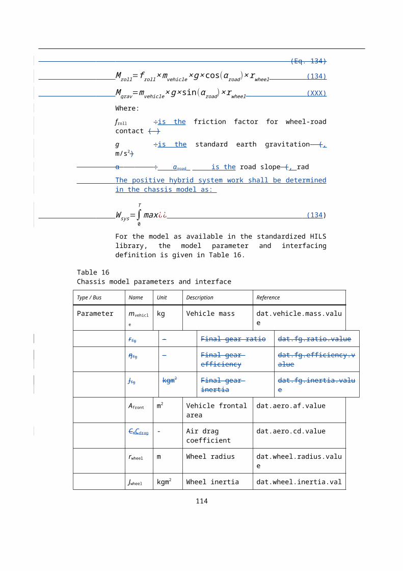
The model shall also implement an inertial load Jretarder to be added to the total powertrain inertia.


Table 26Retarder model parameters and interface


Parameter TlossMretarder,max Nm Retarder brake torque map

dat.braketorque.t-orque.vec

Jretarder kgm2 Inertia dat.inertia.value

Command signal

u - Retarder on/off-control signal between 0-1

Ret_flgOnOff_B

Sensor signal TlossMloss Nm Retarder brake torque

Ret_tqBrkAct_Nm

Mech in [Nm] Min Nm torque phys_torque_Nm

Jin kgm2 inertia phys_inertia_kgm2

Mech out [Nm]



Mech fb in [rad/s]

ωin rad/s rotational speed phys_speed_radps

Mech fb out [rad/s]

ωout rad/s rotational speed phys_speed_radps

A.9.7.7.6. Fixed

Table XXXRetarder model parameters


Mretarder,max Manufacturer specified -

Jretarder Manufacturer specified -

A.9.7.7.6. Spur gear model

A A spur gear transmission or fixed gear transmission with a set of cog wheels and fixed gear ratio shall be represented in accordance with following equation:

ωspur ,out=ωspur ,∈¿ /r spur¿ (168)

114

The gear losses shall be considered as torque losses and implemented through an efficiency asimplemented as function of speed and torque:

❑❑❑❑❑❑❑❑❑❑

(169)

The gear inertias shall be included as:

(Eq. 170)

Jspur , out=J spur ,∈¿r spur2 +J spur ¿ (170)


Table 28Fixed gear model parameters and interface


Parameter JgearJspur kgm2 Inertia dat.in.inertia.value

rgearrspur - Gear ratio dat.in.ratio.value

ηgearηspur - Efficiency dat.in.mechefficiency.effi-ciency.valuemap

Command signal

no signal

Sensor signal no signal

Mech in [Nm]

Min Nm torque phys_torque_Nm


Mech out [Nm]



Mech fb in [rad/s]

ωoutωspur,out rad/s rotational speed phys_speed_radps

Mech fb out [rad/s]

ωinωspur,in rad/s rotational speed phys_speed_radps

115

Table XXXSpur gear model parameters


Jspur Manufacturer specified -

rspur Manufacturer specified -ηspur Manufacturer specified -

A.9.7.7.7. Torque converter model

A torque converter is a fluid coupling device that transfers the input power from its impeller or pump wheel to its turbine wheel on the output shaft through its working fluid motion. A torque converter equipped with a stator will create torque multiplication in slipping mode. A torque converter is often applied as the coupling device in an automatic (shift) transmission.

The torque converter shall transfer the input torque to the output torque ac-cording to two operating phases: slipping and closed.

The torque converter model shall be defined in accordance with following (differential) equations of motion:

(Eq. ❑❑❑❑❑❑❑❑ (171)

The representation of J t ωt=Mt−M out (171)

Where:

Jp is the pump inertia, kgm2

Jt is the turbine inertia, kgm2

ωp is the pump rotational speed, rad/s

ωt is the turbine rotational speed, rad/s

Min is the input torque converter model is shown in Figure 31., Nm

Figure 31

Torque converter model diagram Mout is the output torque, Nm

Mp is the pump torque, Nm

Mt is the turbine torque, Nm

116

The pump torque converter model characteristics shall be definedmapped as function of (rotational) speeds using typical parameters like torque (multi-plication)the speed ratio and efficiency.as:

M p=f pump (ωt/ω p )(ω p/ωref )2 (172a)

Where:

ωref is the reference mapping speed, rad/s

fpump(ωt/ωp) is the mapped pump torque as function of the speed ratio at the constant mapping speed ωref, Nm

The speedturbine torque shall be determined as an amplification of the pump torque as:

M t=f amp (ωt /ω p ) M p (X)

where:

famp(ωt/ωp) is the mapped torque amplification as function of the speed ra-tio

During closed operation, the following relations shall apply:

M out=M ¿−M tc , loss(ωp) (X)

ωt=ωp (X)

where:

Mtc,loss is the torque loss at locked lock-up, Nm

A clutch shall be used to switch between the slipping phase and torque ra-tiosthe closed phase. The clutch shall be modelled in the same way as the clutch device in A.9.7.7.1. During the transition from slipping to closed oper-ation, eqution 172a shall be modified as:

M p=f pump (ωt /ω p )(ω p/ωref )2+ulu M lu ,maxtorque tanh (c (ωp−ωt)) (X)

Where:

Mlu,maxtorque is the maximum torque transfer through the clutch, Nm

ulu is the clutch actuation control signal between 0 and 1

c is a tuning constant for the torque converter model shall be in accordance with:hyperbolic function tanh.

When the speed difference ωp - ωt is below the threshold limit sliplimit and the clutch actuator is above the threshold position ulimit, the clutch is considered not to be slip-ping and shall be considered as locked closed.

117

The lock-up device actuator shall be represented as a first order system:

ulu=−1τ1

× ( ulu−u ) (X)

Where:

ulu is the lock-up actuator position between 0 and 1

u is the desired lock-up actuator position between 0 and 1

τ1 is the time constant


Table 29Torque Converter model parameters and interface

in.value

dat.inertia.out.value

Maximum clutch torquedat.clutch.maxtorque.value

Tuning constant dat.clutch.tanh.value

Slipping clutch, relative speed limit

dat.clutch.speedtolerance.value

Slipping clutch, pedal limitdat.clutch.threshold.value

Time constant actuatordat.clutch.actuator.timeconstant.value

Reference speed dat.characteristics.refspeed.value

Speed ratio mapdat.torqueratiomapdat.characteristics.speedra-tio.vec

dat.characteristics.inputtorque.vec

dat.characteristics.torqueratio.vec

Speed vector for torque loss

dat.characteristics.loss.torque.vec

Command signal Torque converter lockup signal

TC_flgLockUp_B

Sensor signal Pump speed TC_nPumpAct_radps

Pump torque TC_tqPumpAct_Nm

Sensor signal Turbine speed TC_nTurbineAct_radps

Turbine torque TC_tqTurbineAct_Nm

118

Mech in [Nm] phys_torque_Nm

phys_inertia_kgm2

Mech out [Nm] phys_torque_Nm

phys_inertia_kgm2

Mech fb in [rad/s] rotational speed phys_speed_radps

Mech fb out [rad/s] rotational speed phys_speed_radps

Table XXXTorque converter model parameters


J1 Manufacturer specified -

J2 Manufacturer specified -Mlu,maxtorque Manufacturer specified -

c Tuneable default: 0.2sliplimit Tuneable default: 3

ulimit Tuneable default: 0.8fpump Manufacturer specified -

famp Manufacturer specified -Mloss Manufacturer specified -

A.9.7.7.8. Shift transmission model

The shift transmission model shall be implemented as gears in contact, with a specific gear ratio rgear in accordance with:

ωtr ,∈¿=ωtr ,out rgear ¿ (174)

All losses in the transmission model shall be defined as torque losses and im-plemented through a fixed transmission efficiency for each individual gear. The transmission model shall than be in accordance with:

(Eq.

M out={ M ¿r gearηgear , for M ¿≤ 0M ¿r gear /ηgear , for M ¿>0 (175)

The total gearbox inertia shall depend on the active gear selection and is defined with following equation:

119

(Eq. 176)

J gear ,out=J gear ,∈¿ rgear2 + Jgear ,out¿ (176)

For the model as available in the standardized HILS library, the model para-meter and interfacing definition is given in Table 30.26.

The model in the standardized HILS library includes a clutch model. This is used to enable a zero torque transfer during gearshifts. Other solutions are possible. The time duration where the transmission is not transferring torque is defined as the torque interrupt time tinterrupt. This implementation directly links some of the parameters listed in table X to the clutch model as de-scribed in paragraph A.9.8.7.1.

Table 26Shift transmission model parameters and interface


Parameter s Shift time dat.shifttime.value

Nm Maximum torque dat.maxtorque.value

Parameter nrgears - Number of gears dat.nofgear.value

gearnum - Gear numbers (vector)

dat.gear.number.valuevec

Jgearbox kgm2 Inertia (vector) dat.gear.inertia.valuevec

rgear - Gear ratio (vec-tor)

dat.gear.ratio.valuevec

ηgear - Gear efficiency (vectormap)

dat.gear.mechefficiency.effi-ciency.valuemap

Clutch related para-meters

tinterrupt s Shift time dat.torqueinterrupt.value

- Nm Maximum torque dat.maxtorque.value

c - Tuning constant dat.tanh.value

- rad/s Slipping clutch, relative speed limit

dat.speedtolerance.value

Command signal - Requested gear number

Transm_nrGearReq

Sensor signal - Actual gear number

Transm_nrGearAct

boolean Gear engaged Transm_flgConnected_B

ωout rad/s Output speed Transm_nOutAct_radps

120

ωin rad/s Input speed Transm_nInAct_radps

Mech Min Nm torque phys_torque_Nm


Mech out [Nm] Mout Nm torque phys_torque_Nm


Mech fb in [rad/s] ωout rad/s rotational speed phys_speed_radps

mech ωin rad/s rotational speed phys_speed_radps

Table XXXShift transmission model parameters


tinterrupt Manufacturer specified A.9.6.2.X.

gearnum Manufacturer specified Example: 0, 1, 2, 3, 4, 5, 6nrgear Manufacturer specified -

Jgearbox Manufacturer specified -rgear Manufacturer specified -

ηgear Regulated A.9.6.2.X.dat.maxtorque.value Tuneable -

dat.tanh.value Tuneable -dat.speedtolerance.value Tuneable -

A.9.7.8. Rechargeable Energy Storage Systems

A.9.7.8.1. Battery (resistor) model

A resistor basedThe battery model (Figure 32) can be used andbe based on the representation using resistor and capacitor circuits as shown in Figure 34.

121

Figure 34

Representation diagram for RC-circuit battery model

The battery voltage shall satisfy:

(Eq. u❑❑❑❑ (181)

With:

(Eq. 182)

ddt

uRC

=−1RC

uRC+ 1C

i (182)

The open-circuit voltage e, the resistances Ri0 and R and the capacitance C shall all have dependency of the actual energy state of the battery and be modelled using tabulated values in maps. The resistances Ri0 and R and the capacitance C shall have current directional dependency included.

The battery state-of-charge SOC shall be defined as:

SOC=SOC (0 )−∫0

t i3600CAP

dt (X)

Where:

SOC(0) is the initial state of charge at test start

CAP is the battery capacity, Ah

The battery can be scalable using a number of cells.

The battery model can includeprovides a thermodynamics model that may be used and applies similar modelling as for the electric machine system and calculation its losses as followsin accordance with:

(Eq. 183)

Ploss, bat=Ri 0 i2+R iR2=Ri 0i2+

uRC2

R (183)

122

The power losses shall beare converted to heat energy affecting the battery temperature that will be in accordance with:

T bat=1

τbat , heat(Ploss ,bat−( Tbat−Tbat , cool )/ Rbat ,th ) (184)

Where:

Tbat : Battery is the battery temperature (, K)

ΤbatTbat,heat : Time constantis the thermal capacity for battery thermal mass (), J/K

Tbat,cool : Battery is the battery cooling medium temperature (, K)

Rbat,th : Batteryis the thermal resistance ()between battery and cooling fluid, K/W


Table 32Standard RC-based batteryBattery model parameters and interface


Parameter ns - Number of cells connected in series

dat.ns.value

np - Number of cells connected in par-allel

dat.np.value

CAP Ah Cell capacity dat.capacity.value

SOC(0) per cent Initial state of charge

dat.initialSOC.value

e V Open circuit voltage =f(SOC)

dat.ocv.ocv.vec

Ri0 Ω Cell resistance =f(SOC)

dat.resi.charge.R0.vec

dat.resi.discharge.R0.vec

R Ω Cell resistance =f(SOC)

dat.resi.charge.R.vec

dat.resi.discharge.R.vec

C F Cell resistance =f(SOC)

dat.resi.charge.C.vec

dat.resi.discharge.C.vec

Optional para-meters

τbat,heat J/K Thermal capacity dat.cm.value

Rth K/W Thermal resist-ance

dat.Rth.value

123

- - Properties of the cooling fluid

dat.coolingFluid

Command signal no signal

Sensor signal i A Actual current REESS_iAct_A

u V Actual output voltage

REESS_uAct_V

SOC % State of charge REESS_socAct_Rt

Tbat K Battery temper-ature

REESS_tAct_K

Elec out [V] u V Voltage phys_voltage_V

Elec fb in [A] i A Current phys_current_A

Table XXXBattery model parameters


ns Manufacturer specified -

np Manufacturer specified -CAP Regulated A.9.8.8.5.

SOC(0) Manufacturer specified -e Regulated A.9.8.8.5.

Ri0 Regulated A.9.8.8.5.

R Regulated A.9.8.8.5.

C Regulated A.9.8.8.5.

A.9.7.8.2. Capacitor model

A capacitor model shall satisfy:

u¿uC−R i i (X)

where uC is the capacitor voltage and Ri is the internal resistance. The capa-citor voltage shall be determined according to:

uC=−1C ∫ idt (X)

where C is the capacitance.

For a capacitor system the state-of-charge is directly proportional to the capa-citor voltage:

124

SOCcap=uC−V min

V C ,max−V C , min (X)

Where:

VC,min and VC,max are, respectively, the minimum and maximum capacitor voltage.

A diagram for the capacitor model is shown in figure X.

Figure XCapacitor model diagram

The capacitor can be scalable using a number of capacitors connected in parallel and series.

The capacitor model provides a thermodynamics model similar to the battery model.

For the model as available in the standardized HILS library, the model para-meter and interfacing definition is given in table X.

Table XCapacitor model parameters and interface


Parameter ns - Number of cells connected in series

dat.ns.value

np - Number of cells connected in paral-lel

dat.np.value

C F Capacitance dat.C.value

CRi AhΩ Cell capacityresist-ance

dat.capacityR.value

SOCuC(0) %V Initial state of chargecapacitor voltage

dat.initialSOCinitialVoltage.value

eVC,min V Open circuitMin-imum capacitor voltage =f(SOC)

dat.ocv.ocvVmin.value

Ri0VC,max ΩV Cell resistanceMax-imum capacitor

dat.resistance.R0Vmax.value

125

voltage

R Ω Cell resistance dat.resistance.R

C F Cell resistance dat.resistance.C

Command sig-nal

no signal

Sensor signal i A Actual current REESS_iAct_A

u V Actual output voltage

REESS_uAct_V

SOC % State of charge REESS_socAct_Rt

TbatTcapacitor K BatteryCapacitor temperature

REESS_tAct_K

Elec out [V] u V Voltage phys_voltage_V

Elec fb in [A] i A Current phys_current_A

A.9.7.8.3.

Table XXXCapacitor model parameters

Reserved. Parameter Parameter type Reference paragraph

ns Manufacturer specified -np Manufacturer specified -

Vmin Regulated A.9.8.8.6.Vmax Regulated A.9.8.8.6.

uC(0) Manufacturer specified -Ri Regulated A.9.8.8.6.

C Regulated A.9.8.8.6.

A.9.7.8.3. Flywheel model

The flywheel model shall represent a rotating mass that is used to store and release kinetic energy. The flywheel kinetic energy state is defined by:

E flywheel=J flywheel ωflywheel2 (164)

Where:

Eflywheel is the kinetic energy of the flywheel, J

Jflywheel is the inertia of the flywheel, kgm2

ωflywheel is the flywheel speed, rad/s

The basic flywheel model diagram is shown in Figure 30.

126

Figure 30Flywheel model diagram

The flywheel model shall be defined in accordance with following differen-tial equation:

J flywheelddt

ωflywheel=−M flywheel ,∈¿−M flywheel , loss(ωflywheel)¿ (165)

Where:

Mflywheel,in is the input torque to flywheel, Nm

Mflywheel,loss is the (speed dependent) flywheel loss, Nm

The losses may be determined from measurements and modelled using maps.

The flywheel speed shall be restricted by a lower and upper threshold value, respectively, ωflywheel_low and ωflywheel_high:

ωflywheellow≤ ωflywheel ≤ ωflywheel high

(X)


Table 24Flywheel model parameters and interface


Parameter Jfly kgm2 Inertia dat.inertia.valueMloss Nm Torque loss map dat.loss.torqueloss.vec

ωflywheel_low rad/s Lower speed limit

dat.speedlimit.lower.-value

ωflywheel_high rad/s Upper speed limit

dat.speedlimit.upper.-value

Command signal

no signal

Sensor signal ωfly rad/s Flywheel speed Flywheel_nAct_radpsMech in [Nm] Min Nm torque phys_torque_Nm

Jin kgm2 inertia phys_inertia_kgm2Mech fb out [rad/s]

ωfly rad/s rotational speed phys_speed_radps

127

Table XXXFlywheel model parameters


Jfly Manufacturer specified -

Mloss Manufacturer specified -ωflywheel_low Manufacturer specified -

ωflywheel_high Manufacturer specified -

A.9.7.8.4. Accumulator model

A hydraulic accumulator is a pressure vessel to store and release a working medium (either fluid or gas). Commonly, a high pressure accumulator and a low pressure reservoir are part of the hydraulic system. Both the accumulator and reservoir shall be represented using the same modelling approach for which the basis is shown in Figure 35.

Figure 35

Accumulator representation

The accumulator shall be represented in accordance with following equa-tions, assuming ideal gas law, gas and fluid pressure to be equal and no losses in the accumulator:

(Eq. ❑❑❑

(185)

(Eq. 186)

The process shall be assumed to be a reversible adiabatic process:

pgas V gasγ =constant (186)

Where:

mg : charge pgas is the gas mass (kg)pressure, Pa

128

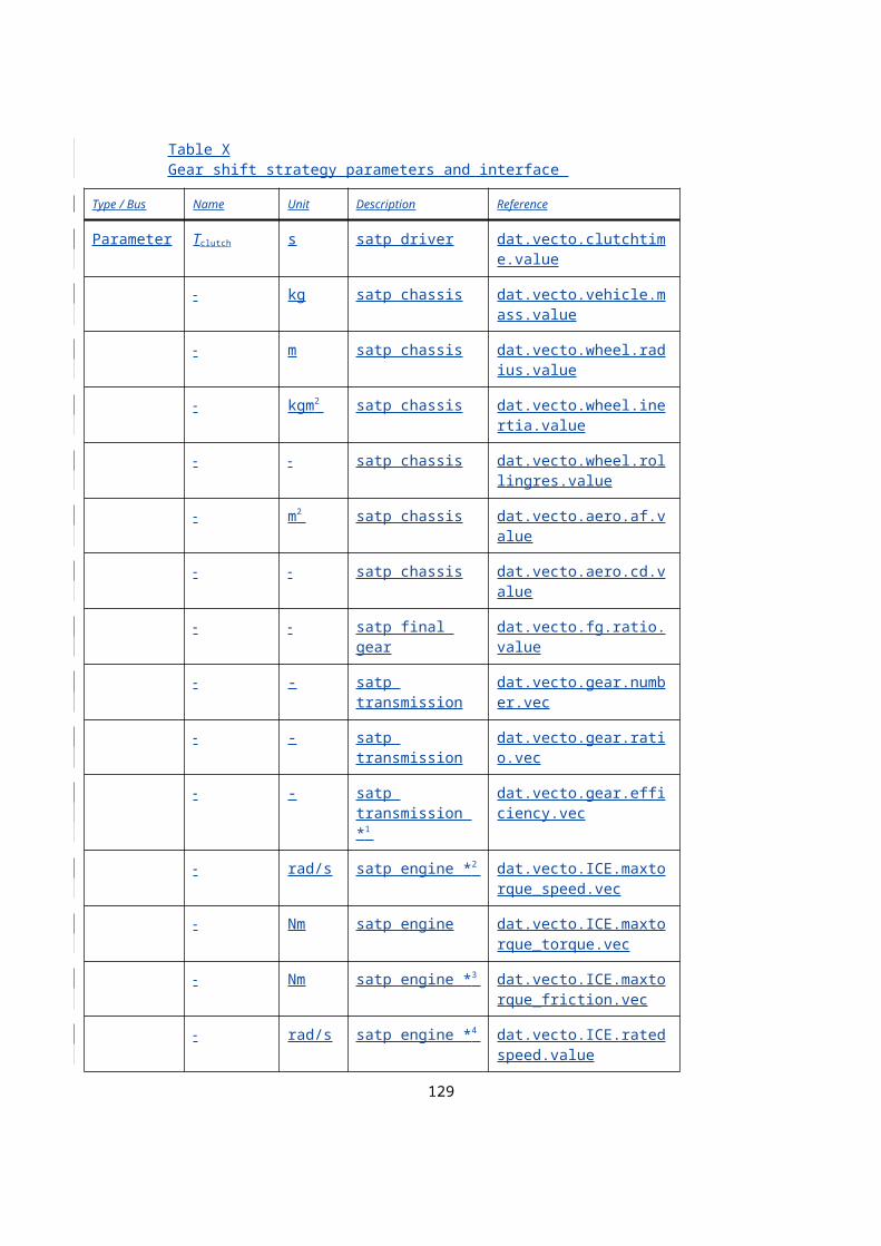
R :Vgas is the gas volume, m3 γ is the adiabatic index

This assumption means that no energy is transferred between the gas and the surroundings.

The constant shall be determined from the precharging of the accumulator:

Tg : charge gas temperature (K)

The model can contain a heat transfer model using following relation:

pgas, pre V gas , preγ =constant (XXX)

Where:

cv : Chargepgas,pre is the precharged gas specificpressure, Pa

Vgas,pre is the precharged gas volume (), m3

h : Accumulator heat transfer coefficient ()

Aw : Accumulator surface area (m2)

Tw : Accumulator surface temperature (K) γ is the adiabatic index

The work done by the pressure-volume changes as a result from this adiabatic process, is equal to:

W =−pgas , pre V gas, pre

γ (V gas1−γ−V gas, pre

1− γ )(1−γ )3600000

(XXX)

and the corresponding state-of-charge shall be determined as:

SOCacc=W

Cacc (XXX)


Table 33Accumulator model parameters and interface


Parameter Tpgas,pre KPa Gas temperat-urePrecharged gas pressure

dat.gas.temperaturepressure.-precharge.value

mgγ kg- Mass of gasAd-iabatic index

dat.gas.massadiabaticindex.-value

R J/kg Gas constant dat.gas.constant.value

VgVgas m3 TankPrecharged dat.capacity.volumevol.pres-

129

volume sure.value

VfCacc m3kWh Fluid volumeAc-cumulator capa-city

dat.capacity.fluid.value

Vgas(0) %m3 Initial fluid volume

dat.capacity.fluid.initvol.ini-tial.value

Command signal no signal

Sensor signal p Pa Pressure Acc_presAct_Pa

Tg K Gas temperature Acc_tGasAct_K

Vg - Gas volume Acc_volGas_Rt

Fluid out [Pa] p Pa Pressure phys_pressure_Pa

Fluid fb in [m3/s] Q m3/s Volume flow phys_flow_m3ps

Table XXXAccumulator model parameters


pgas,pre Manufacturer specified -γ Manufacturer specified -

Vgas,pre Manufacturer specified -Vgas(0) Manufacturer specified -

Cacc Manufacturer specified -

A.9.7.9. Provisions on OEM specific component models

The manufacturer may use alternative powertrain component models that are deemed to at least include equivalent representation, though with better matching performance, than the models listed in paragraphs A.9.7.2. to A.9.7.8. An alternative model shall satisfy the intent of the library model. De-viations from the powertrain component models specified in paragraph A.9.7. shall be reported and be subject to approval by the type approval or certifica-tion authority. The manufacturer shall provide to the type approval or certi-fication authority all appropriate information relating to and including the al-ternative model along with the justification for its use. This information shall be based on calculations, simulations, estimations, description of the models, experimental results and so on.

The chassis model shall be in accordance with paragraph A.9.7.3.

The reference HV model shall be set up in accordance with paragraphs A.9.7.2. to A.9.7.8.

130

A.9.8. Test procedures for energy converter(s) and storage device(s)


The procedures described in paragraphs A.9.8.2. to A.9.8.5. shall be used for obtaining parameters for the HILS system components that is used for the calculation of the engine operating conditions using the HV model.

A manufacturer specific component test procedure may be used in the fol-lowing cases:

(a) Specific component test procedure not available in this gtr;

(b) Unsafe or unrepresentative for the specific component;

(c) Not appropriate for a manufacturer specific component model.

These manufacturer specific procedures shall be in accordance with the intent of specified component test procedures to determine representative data for use of the model in the HILS system. The technical details of these manufac-turer component test procedures shall be reported to and subject to approval by the type approval or certification authority along with all appropriate in-formation relating to and including the procedure along with the justification for its use. This information shall be based on calculations, simulations, es-timations, description of the models, experimental results and so on.

A.9.8.32. Equipment specification

Equipment with adequate characteristics shall be used to perform tests. Re-quirements are defined below and shall be in agreement with the linearity re-quirements and verification of paragraph 9.2.

The accuracy of the measuring equipment (serviced and calibrated according the handling procedures) shall be such that the linearity requirements, given in Table 34 and checked in accordance with paragraph 9.2, are not exceeded.

Table 34Linearity requirements of instruments

Meas |

(fo

Sl

a1

Sta

SE

C

r

Spe ≤ 0.05 % max 0.98 – 1.02 ≤ 2 % max ≥ 0.990

Torque ≤ 1 % max 0.98 – 1.02 ≤ 2 % max ≥ 0.990

Temperatures ≤ 1 % max 0.99 – 1.01 ≤ 1 % max ≥ 0.998

Current ≤ 1 % max 0.98 – 1.02 ≤ 1 % max ≥ 0.998

Voltage ≤ 1 % max 0.98 – 1.02 ≤ 1 % max ≥ 0.998

Power ≤ 2 % max 0.98 – 1.02 ≤ 2 % max ≥ 0.990

131

A.9.8.3. Internal Combustion Engine

The engine torque characteristics, the engine friction loss and auxiliary brake torque shall be determined and converted to table data as the input parameters for the HILS system engine model. The measurements and data conversion shall be carried out in accordance with paragraphs A.9.8.3.1. through A.9.8.3.7.

A.9.8.3.1. Test engine

The test engine shall be the engine of the parent hybrid powertrain in accord-ance with the provision of paragraph 5.3.4.

A.9.8.3.2. Test conditions and equipment

The test conditions and applied equipment shall be in accordance with the provisions of paragraphs 6 and 9, respectively.

A.9.8.3.32. Engine warm-up

The engine shall be warmed up in accordance with paragraph 7.4.1.

A.9.8.3.43. Determination of the mapping speed range

The minimum and maximum mapping speeds are defined as follows:

(a) Minimum mapping speed = idle speed at the warmed-up condition

(b) Maximum mapping speed = nhi x 1.02 or the speed where the full load torque drops off to zero, whichever is smallerrange shall be in accord-ance with paragraph 7.4.2.

A.9.8.3.54. Mapping of positive engine torque characteristics

When the engine is stabilized in accordance with paragraph A.9.8.3.32., the engine torque mapping shall be performed in accordance with the following procedure.

(a) The engine torque shall be measured, after confirming that the shaft torque and engine speed of the test engine are stabilized at a constant value for at least one minute, by reading out the braking load or shaft torque of the engine dynamometer. If the test engine and the engine dynamometer are connected via a transmission, the read-out-value shall be divided by the transmission efficiency and gear ratio of the transmission. In such a case, a (shift) transmission with a known (pre-selected) fixed gear ratio and a known transmission efficiency shall be used and specified.

(b) The engine speed shall be measured by reading the speed of the crank shaft or the revolution speed of the engine dynamometer. If the test engine and the engine dynamometer are connected via a transmission, the read-out-value shall be multiplied by the gear ratio.

(c) The engine torque as function of speed and command value shall be measured under at least 100 conditions in total, for the engine speed under at least 10 conditions within a range in accordance with para-graph A.9.8.3.43, and for the engine command values under at least 10 conditions within a range from 100 per cent to 0 per cent operator command value. The distributionmeasurement points may be equally distributed and shall be defined using good engineering judgement.

132

A.9.8.3.65. Measurement of engine friction and auxiliary brake torque characteristics

After the engine is stabilized in accordance with paragraph A.9.8.3.2., the en-gine friction and auxiliary brake torque characteristics shall be measured as follows:

(a) The measurement of the friction torque of the engine shall be carried out by driving the test engine from the engine dynamometer at un-loaded motoring condition (0 per cent operator command value and effectively realizing zero fuel injection) and performing the measure-ment under at least 10 conditions within a range from maximum to minimum mapping speed in accordance with paragraph A.9.8.3.3. Ad-ditionally, the friction torqueThe measurement points may be equally distributed and shall be measured with an enabled auxiliary brake sys-tem (such as an exhaust brake), if that brake is needed in the HILS system in addition to the engine brakedefined using good engineering judgement.

(b) The engine friction torque including auxiliary braking torque shall be measured by repeating A.9.8.3.6.(a). with all auxiliary brake systems (such as an exhaust brake, jake brake and so on) fully enabled and op-erated at their maximum operator demand. This provision shall not apply if the auxiliary brake systems are not used during the actual powertrain test run for the HILS system verification in accordance with paragraph A.9.5.4.

A.9.8.3.6. Measurement of positive engine torque response

When the engine is stabilized in accordance with paragraph A.9.8.3.2., the engine torque response characteristics shall be measured as follows (and il-lustrated in Figure X).

The engine speeds A, B and C shall be calculated as follows:

Speed A = nlo + 25 %* (nhi – nlo)

Speed B = nlo + 50 %* (nhi – nlo)

Speed C = nlo + 75 % *(nhi – nlo)

(a) The engine shall be operated at engine speed A and an operator com-mand value of 10 per cent for 20 ± 2 seconds. The specified speed shall be held to within ± 20 min-1 and the specified torque shall be held to within ± 2 per cent of the maximum torque at the test speed.

(b) The operator command value shall be moved rapidly to, and held at 100 per cent for 10 ± 1 seconds. The necessary dynamometer load shall be applied to keep the engine speed within ± 150 min-1 during the first 3 seconds, and within ± 20 min-1 during the rest of the segment.

(c) The sequence described in (a) and (b) shall be repeated two times.

(d) Upon completion of the third load step, the engine shall be adjusted to engine speed B and 10 per cent load within 20 ± 2 seconds.

(e) The sequence (a) to (c) shall be run with the engine operating at en-gine speed B.

(f) Upon completion of the third load step, the engine shall be adjusted to engine speed C and 10 per cent load within 20 ± 2 seconds.

(g) The sequence (a) to (c) shall be run with the engine operating at en-gine speed C.

133

(h) Additional sequences (a) to (c) shall be run at selected speed points when selected by the manufacturer.

Figure XEngine positive torque response test

A.9.8.3.7. Engine model torque input data

The tabulated input parameters for the engine model shall be obtained from the recorded data of speed, torque and operator command values as required to obtain valid and representative conditions during the HILS system run-ning. Values equivalent to or lower than the minimum engine speed may be added according to good engineering judgement to prevent non-representat-ive or instable model performance during the HILS system running.

At least 10010 points for torque shall be included in the engine maximum torque table with dependency of at least 10 values for engine speed and at least 10 values for the operatora 100 per cent command value. The distribu-tion may be evenly spread and shall be defined using good engineering judgement. Cubic Hermite interpolation in accordance with Appendix 1 to this annex shall be used when interpolation is required. Values equivalent to or lower than the minimum engine speed may be added to prevent non-rep-resentative or instable model performance during the HILS system running according to good engineering judgement.

At least 10 points for torque shall be included in the engine friction torque table with de-pendency of engine speed and a 0 per cent command value.

At least 10 points for torque shall be included in the engine auxiliary brake torque table with dependency of engine speed and a 0 per cent command valueengine command value and a 100 per cent auxiliary brake system(s) command value. The input values shall be calculated by subtracting the val-ues determined in A.9.8.3.6.(a) from the values determined in A.9.8.3.6.(b) for each set speed. In case the auxiliary brake system(s) are not used during the actual powertrain test run for a HILS system verification in accordance with paragraph A.9.5.4 all values shall be set to zero.

The engine torque response tables with dependency of engine speed shall be determined in accordance with paragraph A.9.8.3.7. and the following pro-

134

cedure for each speed set point (and illustrated in Figure X):

(a) T1 shall be 0.1 seconds or a manufacturer specific value.

(b) The instant torque value shall be the average value of 3 load steps at T1 for each set speed according to A.9.8.3.6.

(c) T2 shall be the time it takes to reach 63% of the difference between the instant torque and the average maximum torque of 3 load steps for each set speed according to A.9.8.3.6.

Figure XEngine torque response parameters

At least 100 points for torque shall be included in the engine torque table with dependency of at least 10 values for engine speed and at least 10 values for the operator command value. The table points may be evenly spread and shall be defined using good engineering judgement. Cubic Hermite interpola-tion in accordance with Appendix 1 to this annex shall be used when inter-polation is required.

A.9.8.4. Electric Machine

A.9.8.4.1. General

The torque map and electric power consumption map of the electric machine shall be determined and converted to table data as the input parameters for the HILS system electric machine model. The test method shall be as pre-scribed and schematically shown in Figure 36.

135

Figure 36Electric machine test procedure diagram

A.9.8.4.2. Test electric machine and its controller

The test electric machine including its controller (high power electronics and ECU) shall be in the condition described below:

(a) The test electric machine and controller shall be serviced in accord-ance with the inspection and maintenance procedures.

(b) The electric power supply shall be a direct-current constant-voltage power supply or (rechargeable) electric energy storage system, which is capable of supplying/absorbing adequate electric power to/from the power electronics at the maximum (mechanical) power of the electric machine for the duration of the test part.

(c) The voltage of the power supply and applied to the power electronics shall be within ± 5 per cent of the nominal voltage of the REESS in the HV powertrain according to the manufacturer specification.

(d) If performance characteristics of the REESS change due to a large voltage variation in the voltage applied to the power electronics, the test shall be conducted by setting at least 3 conditions for the applied voltage: the maximum, minimum and nominal in its control or accord-ing to the manufacturer specification.

(e) The wiring between the electric mchinemachine and its power elec-tronics shall be in accordance with its in-vehicle specifications. How-ever, if its in-vehicle layout is not possible in the test cell, the wiring

136

may be altered within a range not improving the electric machine per-formance. In addition, the wiring between the power electronics and the power supply need not be in accordance with its in-vehicle spe-cifications.

(f) The cooling system shall be in accordance with its in-vehicle specific-ations. However, if its in-vehicle layout is not possible in the test cell, the setup may be modified, or alternatively a test cell cooling system may be used, within a range not improving its cooling performance though with sufficient capacity to maintain a normal safe operating temperature as prescribed by the manufacturer.

(g) No transmission shall be installed. However, in the case of an electric machine that cannot be operated if it is separated from the transmis-sion due to the in-vehicle configuration, or an electric machine that cannot be directly connected to the dynamometer, a transmission may be installed. In such a case, a transmission with a known fixed gear ra-tio and a known transmission efficiency shall be used and specified.


A.9.8.4.3.1. The electric machine and its entire equipment assembly must be conditioned at a temperature of 25 °C ± 5 °C.

A.9.8.4.3.2. The test cell temperature shall remain conditioned at 25 °C ± 5 °C during the test.

A.9.8.4.3.3. The cooling system for the test motor shall be in accordance with paragraph A.9.8.4.2.(f).

A.9.8.4.3.4. The test motor shall have been run-in according to the manufacturer’s recom-mendations.

A.9.8.4.4. Mapping of electric machine torque and power maps

A.9.8.4.4.1. General introduction

The test motor shall be driven in accordance with the method in paragraph A.9.8.4.4.2. and the measurement shall be carried out to obtain at least the measurement items in paragraph A.9.8.4.4.3.

A.9.8.4.4.2. Test procedure

The test motor shall be operated after it has been thoroughly warmed up under the warm-up operation conditions specified by the manufacturer.

(a) The torque output of the test motor shall be set under at least 6 condi-tions on the positive side (‘motor’ operation) as well as the negative side (‘generator’ operation) (if applicable), within a range of the elec-tric machine torque command values between the minimum zero (0 per cent) to the maximum (±100 per cent) or their equivalent com-mand values. (positive and negative). The distributionmeasurement points may be equally distributed and shall be defined using good en-gineering judgement.

137

(b) The test speed shall be set at least 6 conditions between the stopped state (0 rpmmin-1 ) to the maximum design revolution speed as de-clared by the manufacturer. Moreover, the torque may be measured at the minimum motor speed for a stable operation of the dynamometer if its measurement in the stopped state (0 rpm) is difficult. The distri-butionmeasurement points may be equally distributed and shall be defined using good engineering judgement. In case negative speeds are also used on the in-vehicle installation, this procedure may be ex-panded to cover the required speed range.

(c) The minimum stabilized running for each command value shall be at least 3 seconds up to the rated power conditions.

(d) The measurement shall be performed with the internal electric ma-chine temperature and power electronics temperature during the test kept within the manufacturer defined limit values. Furthermore, the motor may be temporarily operated with low-power or stopped for the purpose of cooling, as required to enable continuing the measurement procedure.

(e) The cooling system may be operated at its maximum cooling capacity.

A.9.8.4.4.3. Measurement items

The following items shall be simultaneously measured after confirmed stabil-ization of the shaft speed and torque values:

(a) The shaft torque setpoint and actual value. If the test electric machine and the dynamometer are connected via a transmission, the recorded value shall be divided by the known transmission efficiency and the known gear ratio of the transmission;

(b) The (electric machine) speed setpoint and actual values. If the test electric machine and the dynamometer are connected via a transmis-sion, the electric machine speed may be calculated from the recorded speed of the dynamometer by multiplying the value by the known transmission gear ratio;

(c) The DC-power to/from the power electronics shall be recorded from measurement device(s) for the electric power, voltage and current. The input power may be calculated by multiplying the measured voltage by the measured current;

(d) In the operating condition prescribed in paragraph A.9.8.4.4.2., the electric machine internal temperature and temperature of its power electronics (as specified by the manufacturer) shall be measured and recorded as reference values, simultaneously with the measurement of the shaft torque at each test rotational speed;

(e) The test cell temperature and coolant temperature (in the case of li-quid-cooling) shall be measured and recorded during the test.

A.9.8.4.5. Calculation formulas

The shaft output of the electric machine shall be calculated as follows:

❑❑❑❑❑❑

❑ (188)

Where:

Pem : Electricis the electric machine mechanical power (, kW)

138

Mem : Electricis the electric machine shaft torque (, Nm)

Nem : Electric nem is the electric machine rotational speed (, min-1)

A.9.8.4.6. Electric machine tabulated input parameters

The tabulated input parameters for the electric machine model shall be ob-tained from the recorded data of speed, torque, (operator/torque) command values, current, voltage and electric power as required to obtain valid and representative conditions during the HILS system running. At least 36 points for the power maps shall be included in the table with dependency of at least 6 values for speed and at least 6 values for the command value. This shall be valid for both the motor and generator operation, if applicable. The distribu-tiontable points may be equally distributed and shall be defined using good engineering judgement. Cubic Hermite interpolation in accordance with Ap-pendix 1 to this annex shall be used when interpolation is required. Values equivalent to or lower than the minimum electric machine speed may be ad-ded to prevent non-representative or instable model performance during the HILS system running according to good engineering judgement.

A.9.8.5. Battery

A.9.8.5.1. Resistor based battery model

A.9.8.5.1.1. General

The direct-current internal resistance and open-circuit voltagecharacteristics of the battery shall be determined asand converted to the input parameters for the HILS system battery model and obtained fromin accordance with the bat-tery test. The test method shall be as prescribed and schematically shown be-low in Figure 37:

Figure 37Battery test procedure diagram

measurements and data conversion of paragraphs A.9.8.5.2. through A.9.8.5.15.

A.9.8.5.2. Test battery

The test battery shall be in the condition described below:

(a) The test battery shall be either the complete battery system or a repres-entative subsystem. If the manufacturer chooses to test with a repres-entative subsystem, the manufacturer shall demonstrate that the test results can represent the performance of the complete battery under the same conditions;

(b) The test battery shall be one that has reached its rated capacity C after 5 or less repeated charging / discharging cycles with a current of C/n C, where n is a value between 1 and 3 specified by the battery manu-facturer.

A.9.8.5.1.3. Equipment specification

Measuring devices in accordance with paragraph A.9.8.2. shall be used. In addition, the measuring devices shall comply with following requirements:

A.9.8.5.1.4.(a) temperature accuracy: ≤ 1 °C

(b) voltage accuracy: ≤ 0.2 per cent of displayed reading

139

(c) the resolution of voltage measurement shall be sufficiently small to measure the change in voltage during the lowest applied currents in accordance with the procedures of paragraphs A.9.8.5.5.1., A.9.8.5.5.2. and A.9.8.6.5.

(d) current accuracy: ≤ 0.5 per cent of the displayed reading


(a) The test battery shall be placed in a temperature controlled test cell. The room temperature shall be conditioned at 298 ± 2K (25 ± 2°C) or 318 ± 2K (45 ± 2°C), whatever is more appropriate ac-cording to the manufacturer;

(b) The voltage shall be measured at the terminals of the test battery.

(c) The (c) The battery temperature shall be measured continuously during the test and the temperature measurement shall follow the method specified by the manufacturer or it shall be performed, as shown in Figure 38 below, in the condition not affected by the outside temperature, with the thermometer attached to the central part of the battery and covered with insulation;

(d) The battery cooling system may be either activated or deactivated dur-ing the test.

Figure 38

Battery temperature measurement locations

(left: rectangular battery; right: cylindrical battery)

A.9.8.5.1.5. Current and Battery characteristics test

A.9.8.5.5.1. Open circuit voltage characteristic test

During this test, If the measurement is performed with a representative subsystem the final result is obtained by averaging at least three individual measurements of different subsystems.

(a) After fully charging the test battery in accordance with the charging method specified by the manufacturer, it shall be soaked for at least 12 hours.

(b) The battery temperature at the start of each SOC discharge level shall be 298 ± 2 K (25 ºC ± 2 ºC). However, 318 ± 2 K (45 ºC ± 2 ºC) may be selected by reporting to the type approval or certification authority

140

that this temperature level is more representative for the conditions of the in-vehicle application in the test cycle as specified in Annex 1.b.

(c) The test battery shall be discharged with a current of 0.1C in 5 per cent SOC steps calculated based on the rated capacity specified by the battery manufacturer.

(d) Each time a required 5 per cent SOC discharge level is reached the discharge current is disabled and the test battery is soaked for at least 1 hour, but no more than 4 hours (e.g. by disconnecting the cell). The open circuit voltage (OCV) for this SOC level is measured at the 10th

secondend of the soak time.

(e) When the voltage drops below the minimum allowed limit the dis-charge current is prematurely interrupted and the last soak period starts. The last OCV value corresponds to the empty battery condition. With this definition of the empty battery the actual measured rated ca-pacity of the test battery can be calculated by integrating the recorded discharging and charging with a constant current shall beover time.

(f) Each measured in accordanceOCV value is now assigned to a corres-ponding SOC value based on the actual measured rated capacity of the test battery.

If the measurement is performed with a representative subsystem, data obtained through spline interpolation is used for averaging the individual measurements.

Figure XXX exemplarily shows a typical voltage progress during a complete measurement cycle for a single cell.

Figure XXXExample of typical cell voltage level during the open circuit voltage measurement

141

Figure XXXExample of resulting open circuit voltage as a function of SOC

(measured points are marked with the a dot, spline interpolation is used for data in between measured val-ues)

A.9.8.5.5.2. Test procedure given below: for R0, R and C characteristics

In case the measurement is performed with a representative subsystem, the final results for R0, R and C shall be obtained by averaging at least five indi-vidual measurements of different subsystems.

All SOC values used shall be calculated based on the actual measured rated capacity of the test battery determined in accordance with paragraph A.9.8.5.5.1.

The current and voltage over time shall be recorded at a sampling rate of at least 10 Hz.

(a) The test shall be conducted by changing the depth of discharge (100 per cent - SOC) withinfor at least 5 different levels of SOC which shall be set in such a way as to allow for accurate interpolation. The selected levels of SOC shall at least cover the range used for the test cycle as specified in Annex 1.b. The depth-of-discharge shall be level 3 or more, and shall be set in such a way as to allow for interpolation.

(b) As for the depth of discharge, after After fully charging the battery at an ambient temperature of 298 ± 2 K (25 ºC ± 2 ºC)test battery in ac-cordance with the charging method specified by the manufacturer, it shall be soaked under the same condition for at least 1 hour, but lessno more than 4 hours.

(c) The adjustment of the desired SOC before starting the test sequence shall be performed by changingdischarging or charging the discharge timetest battery with a constant current In (C/n according to paragraph A). The depth of discharge (a per cent) is.9.8.5.2.

(d) After the state after discharging adjustment of the desired SOC, the test battery at In (A)shall be soaked for (0.01 × a × n)at least 1 hour, but no more than 4 hours. However, adjustment may be made by using

142

the immediately preceding actually-measured battery capacity to cal-culate the discharge time for obtaining the targeted depth of discharge. Furthermore, if, after the completion of the current and voltage char-acteristic test at the first depth of discharge, an adjustment to the next depth of discharge is continuously performed, the adjustment may be made by calculating the discharge time from the present depth of dis-charge and the next depth of discharge.

(c(e) The battery temperature at the start of theeach test sequence shall be 298 ± 2 K (25 ºC ± 2 ºC). However, 318 ± 2 K (45 ºC ± 2 ºC) may be selected by reporting in the to the type approval or certifica-tion authority that this temperature level is more representative for the conditions of the in-vehicle application the actually-measured battery temperature at the time ofin the test cycle as specified in Annex 1.b. running equivalent to the in-vehicle condition.

(d) After adjusting the depth of discharge, soak the battery at the pre-scribed battery temperature at the start of the test. The test shall be started 1 hour or more but not more than 4 hours thereafter, and 16 hours or more but not more than 24 hours thereafter in the case of 45ºC.

(e) The test(f) The test sequence at each SOC level shall be conducted in accordance with the sequence listed in Table XXX and shown in Figure 39:XXX.

Figure 39

Test sequence of current-voltage characteristic test

(Example: when for rated capacity below 20Ah) (f) The battery voltage at highest value of the 10th second shall be

measured bycharging and discharging and charging at each current specified for each category of the rated capacity posted in Table 35 below. The upper limit of the charging or discharging current shall be 200 (A) but at least higher thancurrent Imax for the test battery shall be the maximum value used in the HVin-vehicle application of the hybrid powertrain under test as defined by the manufacturer. However, if the battery voltage at the 10th second exceeds the lower limit of The lower step values of the charging and discharging current shall be calculated from this maximum value by successively dividing it by a factor of three for three times (e.g. Imax = 27A gives a sequence for the charging and discharging voltage or the upper limit of charging voltage, that measurement data shall be discarded. current pulses of 1, 3, 9 and 27A).

Table 35Charge/Discharge current values for test

Category of rated capacity Charge / Discharge current

Less than 20Ah ⅓∙n∙In n∙In 5∙n∙In 10∙n∙In Imax

20Ah or more ⅓∙n∙In n∙In 2∙n∙In 5∙n∙In Imax

(g) During the no-load period, the battery shall be cooled off for at least 10 minutes. It shall be confirmed that the change of temperature

143

is kept within ± 2 ºCK before continuing with the next discharging or charging level. current step.

Table XXXTest sequence at each SOC level

Step Action

1 Discharge for 10 seconds with Imax/33

2 No-load period for at least 10 minutes

3 Charge for 10 seconds with Imax/33










13 Discharge for 10 seconds with Imax


15 Charge for 10 seconds with Imax

144

Figure XXXTest sequence at each SOC level

(g) For each discharging and charging current level specified in Table XXX, the no-load voltage before the start of the current pulse Vstart, and the voltages at 1, 5 and 9 seconds after the pulse has started (V1, V5 and V9) shall be measured (shown in Figure XXX).

If the voltage signal contains signal noise, low-pass filtering of the signal or averaging of the values over a short time frame of ± 0.05 - 0.1 seconds from the respective voltage value may be used.

If a voltage value exceeds the lower limit of discharging voltage or the upper limit of charging voltage, that measurement data shall be dis-carded.

145

Figure XXXExample of single voltage pulse during a discharge pulse

A.9.8.5.1.65.3. Calculation of direct-current internal resistance and open-circuit voltage R0, R and C

The measurement data obtained in accordance with paragraph A.9.8.5.4.1.5.2. shall be used to calculate the currentR0, R and voltage charac-teristics fromC values for each charging and discharging current level at each SOC level by using the following equations:

V ∞=V 1× V 9−V 5

2

V 1−2× V 5+V 9

(XXX)

τ=−4

ln (1−(V 9−V 5 )/ (V ∞−V 5 )) (XXX)

For a charge pulse:

K=−τ × ln (1−V 1/V ∞ ) (XXX)

V 0=V ∞× (1−e( 1−K )/ τ ) (XXX)

For a discharge pulse:

V 0=V 1−V ∞

e−1/ τ +V ∞ (XXX)

The values for R0,pulse, Rpulse and Cpulse for a specific current level Ipulse shall be calculated as:

R0 , pulse=V 0−V start

I pulse (XXX)

146

Rpulse=V ∞−V 0

I pulse (XXX)

C pulse=τ

Rpulse (XXX)

The required values for R0, R and C for, respectively, discharging currents and their corresponding voltages. charging or discharging at one specific SOC level shall be calculated as the mean values of the all the corresponding charging or discharging current levels. The same calculations shall be per-formed for all selected levels of SOC in order to get the specific values for R0, R and C not only depending on charging or discharging, but also on the SOC.

The method A.9.8.5.5.4. Correction of R0 for battery subsystems

In case the least-squares shall be used to determinemeasurement is performed with a representative subsystem the best-fit equation havingfinal results for all R0 values may be corrected if the form: internal connections between the subsystems have a significant influence on the R0 values.

y=a× x+b (Eq. 189)

Where:

y = actual value of voltage (V)

x = actual value of current (A)

a = slope of the regression line

b = y-The validity of the values used for correction of the original R0 values shall be demonstrated to the type approval or certification authority by calcu-lations, simulations, estimations, experimental results and so on.

A.9.8.6. Capacitor

A.9.8.6.1. General

The characteristics of the (super)capacitor shall be determined and converted to the input parameters for the HILS system supercapacitor model in accord-ance with the measurements and data conversion of paragraphs A.9.8.6.2. through A.9.8.6.7.

The characteristics for a capacitor are hardly dependent of its state of charge or current, respectively. Therefore only a single measurement is prescribed for the calculation of the model input parameters.

A.9.8.6.2. Test supercapacitor

The test supercapacitor shall be either the complete supercapacitor system or a representative subsystem. If the manufacturer chooses to test with a repres-entative subsystem, the manufacturer shall demonstrate that the test results can represent the performance of the complete supercapacitor under the same conditions;

A.9.8.6.3. Equipment specification

Measuring devices that meet the requirements in accordance with paragraph A.9.8.5.3. shall be used.


147

(a) The test supercapacitor shall be placed in a temperature controlled test cell. The room temperature shall be conditioned at 298 ± 2 K (25 ± 2 °C) or 318 ± 2 K (45 ± 2 °C), whatever is more appropriate according to the manufacturer;

(b) The voltage shall be measured at the terminals of the test supercapa-citor.

(c) The supercapacitor cooling system may be either activated or deactiv-ated during the test.

A.9.8.6.5. Supercapacitor characteristics test

In case the measurement is performed with a representative subsystem, the fi-nal result is obtained by averaging at least three individual measurements of different subsystems.

(a) After fully charging and then fully discharging the test supercapacitor to its lowest operating voltage in accordance with the charging method specified by the manufacturer, it shall be soaked for at least 2 hours, but no more than 6 hours.

(b) The supercapacitor temperature at the start of the test shall be 298 ± 2 K (25 ± 2 ºC). However, 318 ± 2 K (45 ± 2 ºC) may be selected by re-porting to the type approval or certification authority that this temper-ature level is more representative for the conditions of the in-vehicle application in the test cycle as specified in Annex 1.b.

(c) After the soak time, a complete charge and discharge cycle according to Figure XXX with a constant current Itest shall be performed. Itest

shall be the maximum allowed continuous current for the test superca-pacitor as specified by the manufacturer or the maximum continuous current occurring in the in-vehicle application.

(d) After a waiting period of at least 30 seconds (t0 to t1), the supercapa-citor shall be charged with a constant current Itest until the maximum operating voltage Vmax is reached. Then the charging shall be stopped and the supercapacitor shall be soaked for 30 seconds (t2 to t3) so that the voltage can settle to its final value Vb before the discharging is started. After that the supercapacitor shall be discharged with a con-stant current Itest until the lowest operating voltage Vmin is reached. Af-terwards (from t4 onwards) there shall be another waiting period of 30 seconds until the voltage will settle to its final value Vc.

(e) The current and voltage over time, respectively Imeas and Vmeas, shall be recorded at a sampling rate of at least 10 Hz.

(f) The following characteristic values shall be determined from the measurement (illustrated in Figure XXX):

Va is the no-load voltage right before start of the charge pulse

Vb is the no-load voltage right before start of the discharge pulse

Vc is the no-load voltage recorded 30 seconds after the end of the dis-charge pulse

∆V(t1), ∆V(t3) are the voltage changes directly after applying the con-stant charging or discharging current Itest at the time of t1 and t3, re-spectively. These voltage changes shall be determined by applying a linear approximation to the voltage characteristics as defined in detail A of Figure XXX by usage of the least squares method.

148

∆V(t1) is the absolute difference of voltages between Va and the intercept value of the regression linestraight-line approximation at the time of t1.

(a) For∆V(t3) is the discharge pulses, calculate the direct-current internal resistance Rd (i.e. absolute valuedifference of the slope)voltages be-tween Vb and the open-circuit voltage Vd0 (i.e. the y-intercept ) from the data (displayed in Figure 40).

(b) For the charge pulses, calculate the direct-current internal resistance Rc (i.e. absolute value of the slope) and the open-circuit voltage Vc0

(i.e. the y-intercept) from the data (displayed in Figure 41).

(c) The open-circuit voltage V0 as input parameter for the model shall be the calculated averagestraight-line approximation at the time of Vd0 and Vc0. t3.

(d) When a single internal resistance parameter is used as input parameter for the model, the direct-current internal resistance R0 shall be the cal-culated average of Rd and Rc. Separate charge and discharge internal resistances may be used.

(e) In case a REESS subsystem is used for the test, the representative sys-tem values ∆V(t2) is the absolute difference of voltages between Vmax and Vb.

∆V(t4) is the absolute difference of voltages between Vmin and Vc.

Figure XXXExample of voltage curve for the supercapacitor measurement

A.9.8.6.6. Calculation of R and C

The measurement data obtained in accordance with paragraph A.9.8.6.5. shall be used to calculate the R and C values according as follows.

(a) The capacitance for charging and discharging shall be calculated as follows:

For charging:

149

C charge=

∑t1

t2

I meas Δt

V b−V a

(XXX)

For discharging:

Cdischarge=

∑t 3

t 4

I meas Δt

V c−V b

(XXX)

(b) The internal resistance for charging and discharging shall be calcu-lated. as follows:

Figure 40Determination of the Internal Resistance and Open-Circuit Voltage during Discharging

Figure 41Determination of the Internal Resistance and Open-Circuit Voltage during Charging

A.9.8.5.2. RC-based battery model

Reserved.

A.9.8.6. Capacitor

Reserved.

For charging:

Rcharge=∆ V (t 1)+∆ V (t2 )

2 I test

(XXX)

For discharging:

Rdischarge=∆ V (t 3 )+∆ V (t 4 )

2 I test

(XXX)

(c) For the model, only a single capacitance and resistance are needed and these shall be calculated as follows:

Capacitance C:

C=Ccharge+Cdischarge

2 (XXX)

Resistance R:

R=Rcharge+Rdischarge

2 (XXX)

A.9.8.6.7. Correction of resistance of supercapacitor subsystems

In case the measurement is performed with a representative subsystem the fi-nal results for the system resistance value may be corrected if the internal connections between the subsystems have a significant influence on the res-istance value.

150

The validity of the values used for correction of the original resistance values shall be demonstrated to the type approval or certification authority by calculations, simulations, estimations, experimental results and so on.

151

Appendix 1 Cubic Hermite interpolation procedure

Reserved. The Hermite interpolation method approximates each of the in-tervals with a third order polynomial expression similar to spline interpola-tion. Hermite interpolation however creates continuous derivatives at con-necting points through first derivatives.

The Hermite interpolation polynomial coincides with the given function value and the derivative of the point.

The interpolation polynomial between the interval of [(x i, yi), (xi+1, yi+1)] is defined in equation (X1), where the equation is cubic polynomial based on the point of (xi, yi).

f ( x )=a× ( x−x i )3+b × ( x−xi )

2+c× ( x−xi )+d (X1)

Since the Hermite interpolation polynomial coincides with the given function value and the derivative of the point, following conditions result:

f ( x i )= y i=d (X2)

f ' ( x i )= y i '=c (X3)

If Δx = xi+1 – xi , then:

f ( x i+1)= y i+1=a × Δ x3+b × Δ x2+ y i ' × Δ x+ y i (X4)

f ' ( x i+1 )= y i+1 '=3 ×a× Δ x2+2 × b× Δ x+ y i ' (X5)

Combining equation X4 and X5 yields:

a=y i+1

' + y i'

Δ x2 −2×y i+1− y i

Δ x3 (X6)

b=− y i+1

' +2× y i'

Δx+3×

y i+1− y i

Δ x2 (X7)

The derivatives used in equations X3, X6, and X7 can be calculated as fol-lows:

y '=| yi+1− y i

xi+1−x i|×|y i− y i−1

xi−xi−1|

(2 × x i+1−xi−xi−1

3× ( x i+1−x i−1 ) )×( y i+1− y i

x i+1−x i )+( x i+1+x i−2× x i−1

3× ( x i+1−x i−1 ) )×( y i− y i−1

xi−xi−1 ) (X8)

152

Annex 10., amend to read

Annex 10

Test procedure for engines installed in hybrid vehicles using the powertrain method

A.10.1. This annex contains the requirements and general description for testing en-gines installed in hybrid vehicles using the Powertrain method.

A.10.2. Test procedure

This annex describes the procedure for simulating a chassis test for a pre-transmission or post-transmission hybrid system in a powertrain test cell. Following steps shall be carried out:

A.10.2.1 Powertrain method

The Powertrain method shall follow the general guidelines for execution of the defined pro-cess steps as outlined below and shown in the flow chart of Figure 42. The details of each step are described in the relevant paragraphs. Deviations from the guidance are permitted where appropriate, but the specific requirements shall be mandatory.

For the Powertrains method, the procedure shall follow:

(a) Selection and confirmation of the HDH object for approval;

(b) Set up of Powertrain system;

(c) Hybrid system rated power mapping;determination

(d) Exhaust emission test;

(e) Data collection and evaluation;

(f) Calculation of specific emissions.

153

Figure 42Powertrain method flow chart

A.10.2.2. Build of the Powertrain system setup

The Powertrain system setup shall be constructed in accordance with the provisions of paragraph A.10.3. and A.9.7. of the HILS method.

A.10.2.3. System Power Mapping Hybrid system rated power determination

The hybrid system rated power shall be determined in accordance with paragraph A.10.4.

A.10.2.4. Powertrain Exhaust Emission Testexhaust emission test

The Powertrain Exhaust Emission Testpowertrain exhaust emission test shall be carried out in accordance with all provisions of paragraph A.10.5.

A.10.3. Set up of powertrain system

A.10.3.1 General introduction

The powertrain system shall consist of, as shown in Figure 43, a HV model and its input parameters, the test cycle as defined in Annex 1.b., as well as the complete physical hybrid powertrain and its ECU(s) (hereinafter referred to as the "ac-tual powertrain") and a power supply and required interface(s). The power-train system setup shall be defined in accordance with paragraph A.10.3.2. through A.10.3.5. The HILS component library (paragraph A.9.7.) shall be applied in this process. The system update frequency shall be at least 100 Hz to accurately control the dynamometer.

154

Figure 43:

Outline of powertrain system setup

A.10.3.2. Powertrain system hardware

The powertrain system hardware shall have the signal types and number of channels that are required for constructing the interface between all hardware required for the functionality of and to connect the dynamometer and the actual power-train.

A.10.3.3. Powertrain system interface

The powertrain system interface shall be specified and set up in accordance with the re-quirements for the (hybrid) vehicle model (paragraph A.10.3.5.) and required for the operation of the dynamometer and actual powertrain. In addition, spe-cific signals can be defined in the interface model to allow proper operation of the actual ECU(s), e.g. ABS signals. All modifications or signals shall be documented and reported to the type approval authorities or certification agency.

The interface shall not contain key hybrid control functionalities as specified in paragraph A.9.3.4.1. of the HILS method.

The actual dynamometer torque shall be used as input to the HV model.

The calculated rotational input speed of the HV model (e.g. transmission or final gear input shaft) shall be used as setpoint for the dynamometer speed.

A.10.3.4. Actual powertrain

The powertrain including all of its ECU(s) in accordance with the in-vehicle installation shall be used for the powertrain system setup. The provisions for setup shall follow paragraph 6.3. of this gtr.

155

The torque measuring device shall be rigidly mounted closely to the hybrid system output shaft. For example, if a damper is needed it should be mounted on the dynamometer and its damping characteristic should not affect the torque reading.

A.10.3.5. Vehicle model

A vehicle model shall represent all relevant characteristics of the applicable hybrid vehicle for the drivetrain and chassis and contain those components not present in the actual powertrain system.(paragraph A.10.3.4.). The HV model shall be constructed by defining its components in accordance with paragraph A.9.7. of the HILS method. The relevant characteristics are defined as:

(a) Chassis (paragraph A.9.7.3.) to determine actual vehicle speed as function of powertrain torque and brake torque, tyretire rolling resist-ance, air drag resistance and road gradients. TheFor validation pur-pose, the actual vehicle speed shall be compared with the desired vehicle speed defined in the test cycle of Annex 1.b.

(b) Final gear (paragraph A.9.7.7.6.) to represent the differential gear functionality, unless it is already included in the actual powertrain.

(c) In case of a manual transmission, the transmission (A.9.7.7.8.) and clutch model (A.9.7.7.1.) may be included as part of the HV model.

The input parameters for the HV model shall be defined in accordance with paragraph A.10.5.2.

A.10.3.6. Driver model

The driver model shall contain all required tasks to drive the HV model over the test cycle and typically includes e.g. accelerator and brake pedal signals as well as clutch and selected gear position in case of a manual shift transmis-sion. The driver model shall use actual vehicle speed for comparison with the desired vehicle speed defined in accordance with the test cycle of Annex 1.b.

The driver model tasks shall be implemented as a closed-loop control. and shall be in accordance with paragraph A.9.7.4.

The shift algorithm for the manual transmission shall be in accordance with paragraph A.9.7.4.(b)..3.

A.10.4. System Hybrid system rated power mapping proceduredetermination

A.10.4.1. General

The purpose of the mapping procedure in this paragraph is to determine the maximum hy-brid system torque andrated power available at each speed with a fully/suffi-ciently charged Rechargeable Energy Storage System. One of the following methods shall be used to generate a hybrid-active map.

A.10.4.2 Mapping conditions

Internal Combustion Engines as part of a hybrid system shall be mapped as describeddetermined in this accordance with paragraph when either the HILS method (annex 8. to this gtr) or the Powertrain method (annex 9. to this gtr) are used to determine their exhaust gas pollutant emissions. These provisions may be applied to other types of hybrid engines, consistent with good engi-neering judgment. The mapping procedure as given in paragraph 7.4 of this gtr shall be used except as noted in this paragraph. The powertrain map shall be generated with the hybrid system activated as described in paragraphs A.10.4.3. or A.10.4.4. of this sectionA.9.6.3.

156

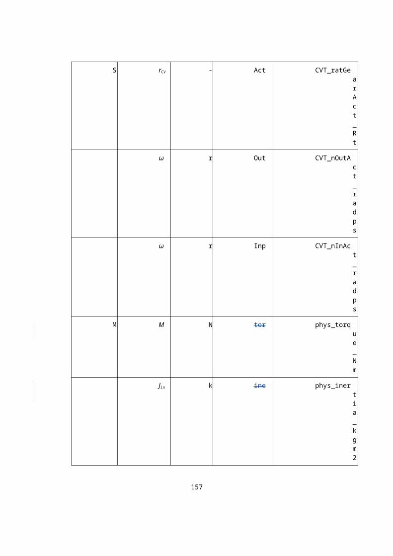
The operator command and speed setpoints may be defined as in standard en-gine testing.

A.10.4.3. Continuous sweep mapping

A powertrain map shall be performed by using a (series of) continuous sweeps to cover the powertrain's full range of operating speeds. The powertrain shall be prepared for hybrid-active mapping by ensuring that the RESS state of charge is repre-sentative of normal operation. The sweep shall be performed as specified in paragraph 7.4 of this gtr, but the sweep shall be stopped to charge the RESS when the power measured from the RESS drops below the expected maxi-mum power from the RESS by more than 2 per cent of total declared system power (including engine and RESS power).

Unless good engineering judgment indicates otherwise, it may be assumed that the ex-pected maximum power from the RESS is equal to the measured RESS power at the start of the sweep segment. For example, if the 3-second rolling average of total engine-RESS power is 200 kW and the power from the RESS at the beginning of the sweep segment is 50 kW, once the power from the RESS reaches 46 kW, the sweep shall be stopped to charge the RESS. Note that this assumption is not valid where the hybrid motor is torque-lim-ited. Total system power shall be calculated as a 3-second rolling average of instantaneous total system power.

After each charging event, the engine shall be stabilized for 15 seconds at the speed at which the previous segment ended with operator demand set to maximum be-fore continuing the sweep from that speed. The cycle of charging, mapping, and recharging shall be repeated until the engine map is completed. The sys-tem may be shut down or other operation may be included between segments to be consistent with the intent of this paragraph. For example, for systems in which continuous charging and discharging can overheat batteries to an ex-tent that affects performance, the engine may be operated at zero power from the RESS for enough time after the system is recharged to allow the batteries to cool. Good engineering judgment shall be used to smooth the torque curve to eliminate discontinuities between map intervals.

A.10.4.4. Discrete speed mapping

A powertrain map shall be performed by using discrete speeds along its full load curve from minimum to maximum mapping speed with increments no greater than 100 min-1. Speed set points shall be selected at at least 13 equally spaced powertrain speeds. Mapping may be stopped at the highest speed above max-imum power at which 50 per cent of maximum power occurs. Powertrain speed shall be stabilized at each setpoint, targeting a torque value at 70per cent of peak torque at that speed without hybrid-assist. The engine shall be fully warmed up and the RESS state of charge shall be within the normal op-erating range. The operator demand shall be moved to maximum, the power-train shall be operated there for at least 10 seconds, and the 3-second rolling average feedback speed and torque shall be recorded at 1 Hz or higher. The peak 3-second average torque and 3-second average speed shall be recorded at that point. Linear interpolation shall be used to determine intermediate speeds and torques. Paragraph 7.4.2. to this gtr shall be followed to calculate the maximum test speed. The measured maximum test speed shall fall in the range from 92 to 108per cent of the estimated maximum test speed. If the measured maximum test speed does not fall in this range, the map shall be re-run using the measured value of maximum test speed.In addition following conditions shall be respected:

157

(a) The hybrid powertrain shall be warmed up to its normal operating condition as specified by the manufacturer

(b) Prior to starting the test, the system temperatures shall be within their normal operating conditions as specified by the manufacturer

(c) The test cell shall be conditioned between 20 °C and 30 °C

A.10.5. Powertrain exhaust emission test


Using the powertrain system setup and all required HV model and interface systems enabled, exhaust emission testing shall be conducted in accordance with the provisions of paragraphs A.10.5.2. to A.10.5.6. Guidance on test se-quence is provided in the flow diagram of Figure 44.

Figure 44

Powertrain exhaust emission test sequence

A.10.5.2. Generic vehicle

Generic vehicle parameters shall be used in the HV model and defined in ac-cordance with paragraphs A.10.5.2.1. to A.10.5.2.6. in case the respective components are not present in hardware during the powertrain test.

158

A.10.5.2.1. Test vehicle mass and curb mass

TestThe test vehicle mass mvehicle and curb mass mvehicle,0 areshall be defined with equation 112 using the hybrid system rated power in accordance with equations 112 and 113 or 114, respectively.paragraph A.10.4.

A.10.5.2.2. Air drag coefficients

The generic vehicle air drag coefficients Afront and Cdrag are calculated in ac-cordance with equations 115 and 116 or 117, respectively.

A.10.5.2.3. TyreTire rolling resistance coefficient

The tyretire rolling resistance coefficient froll is calculated in accordance with equation 118.


The wheel radius shall be defined in accordance with paragraph A.9.5.6.9.

A.10.5.2.5. Final gear ratio and efficiency

The final gear ratio and efficiency shall be defined in accordance with para-graph A.9.6.2.10.


The efficiency of each gear shall be set to 0.95.

A.10.5.2.7. Transmission gear ratio

The gear ratios of the (shift) transmission shall have the manufacturer spe-cified values for the test hybrid powertrain.

A.10.5.2.8. Transmission gear inertia

The inertia of each gear of the (shift) transmission shall have the manufac-turer specified value for the test hybrid powertrain.


For the maximum transmitted torque of the clutch and the synchronizer, the design value specified by the manufacturer shall be used.


The gear-change period for a manual transmission shall be set to one (1.0) second.


Gear positions at the start, acceleration and deceleration during the approval test shall be the respective gear positions defined by the shift strategy in ac-cordance with paragraph A.9.7.4. and shall be part of the driver model.

A.10.5.2.12. Inertia of rotating sections

The inertia for the post transmission parts shall be defined in accordance with paragraph A.9.6.2.15.

In case a post transmission component is included in the actual hardware (e.g. final gear), this specific component inertia as specified by the manufacturer shall be used to correct the inertia as specified in accordance with paragraph A.9.6.2.15. taking into account the gear ratios between this component and the wheels. The resulting post transmission inertia shall have a minimum value of 0 kgm2 .

159


All other input parameters shall have the manufacturer specified value for the actual test hybrid powertrain.

A.10.5.3. Data to be recorded

All data required to allow for the checks of speed, net energy balance and de-termination of emissions shall be recorded at 5 Hz or higher (10 Hz recom-mended).

A.10.5.4. Emission test sequence

The test sequence shall be in accordance with paragraph 7.6.

A.10.5.5. Validation statistics

For each test, either cold or hot started, it shall be valid if the test conditions of paragraph A.10.5.5.1. and A.10.5.5.2. are met.

A.10.5.5.1. Validation of vehicle speed

The criteria for vehicle speed and net energy change of the RESS shall be in accordance with paragraph A.9.6.4.4.

A.10.5.5.2. Validation of RESS net energy change

The ratio of RESS net energy change to the cumulative fuel energy value shall satisfy the following equation:

(Eq. |❑❑| (190)

Where:

ΔE : Net is the net energy change of the RESS in accordance with para-graph A.9.5.8.2.3.(a)-(d), kWh

Ctest : Energy is the energy value for the cumulative amount of fuel mass flow during test, kWh

A.10.A.9. In case the net energy change criterion is not met, the powertrain system shall be readied for another test run.

A.10.5.6.25.3. Validation of dynamometer speed

Linear regression of the actual values for the dynamometer speed on the ref-erence values shall be performed for each individual test cycle. The method of least squares shall be used, with the best-fit equation having the form:

(Eq. ❑❑❑❑ (191)

Where:

y :is the actual value of speed (, min-1)

x :is the reference value of speed (, min-1)

a1 :is the slope of the regression line

a0 :is the y-intercept value of the regression line

The standard error of estimate (SEE) of y on x and the coefficient of determ-ination (r2) shall be calculated for each regression line.

For a test to be considered valid, the criteria of Table 36 shall be met.

160

Table 36Statistical criteria for speed validation

Parameter Speed control

Slope, a1 0.950 ≤ a1 ≤ 1.030Absolute value of intercept, |a0| ≤ 2.0 % of maximum test speed

Standard error of estimate, SEE ≤ 5.0 % of maximum test speedCoefficient of determination, r2 ≥ 0.970

A.10.6. Data collection and evaluation

Reserved.

In addition to the data collection of gtr4 (in accordance with paragraph 7.6.6), the hybrid system work shall be determined over the test cycle by synchron-ously using the hybrid system rotational speed and torque values at the wheel hub (HV chassis model output signals in accordance with paragraph A.9.7.3.) recorded during the test in accordance with paragraph A.10.5. to calculate in-stantaneous values of hybrid system power. Instantaneous power values shall be integrated over the test cycle to calculate the hybrid system work Wsys_test

(kWh). Integration shall be carried out using a frequency of 5 Hz or higher (10 Hz recommended) and include only positive power values.

The hybrid system work Wsys shall be calculated as follows:

W sys=W systest×( 1

0.95 )2

(X)

Where:

Wsys is the hybrid system work, kWh

Wsys_test is the hybrid system work from the test run, kWh

All parameters shall be reported.

A.10.7. Calculation of the specific emissions

Reserved.

The specific emissions egas or ePM (g/kWh) shall be calculated for each indi-vidual component as follows:

e=m

W sys (109)

Where:

e is the specific emission, g/kWh

m is the mass emission of the component, g/test

Wsys is the cycle work as determined in accordance with paragraph A.10.6., kWh

The final test result shall be a weighted average from cold start test and hot start test in accordance with the following equation:

161

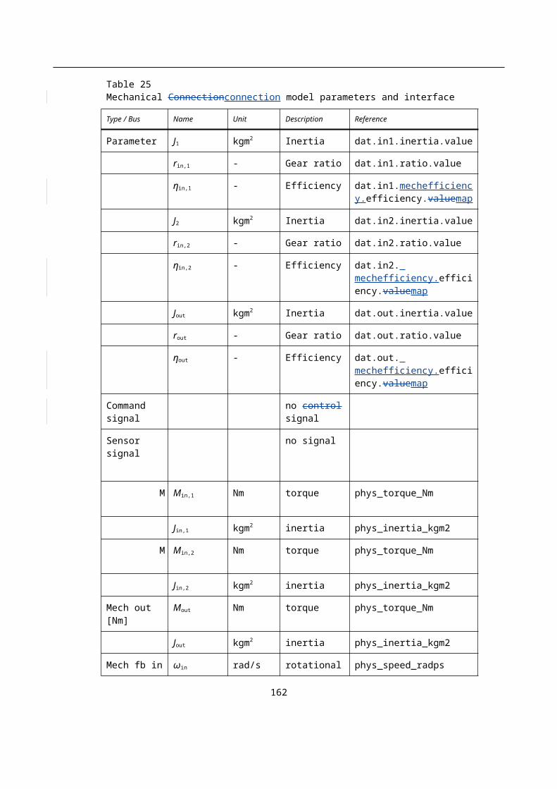
e=(0.14 ×mcold)+(0.86 × mhot)

(0.14 ×W sys ,cold)+(0.86 × W sys , hot) (110)

Where:

mcold is the mass emission of the component on the cold start test, g/test

mhot is the mass emission of the component on the hot start test, g/test

Wsys,cold is the hybrid system cycle work on the cold start test, kWh

Wsys,hot is the hybrid system cycle work on the hot start test, kWh

If periodic regeneration in accordance with paragraph 6.6.2. applies, the re-generation adjustment factors kr,u or kr,d shall be multiplied with or be added to, respectively, the specific emission result e as determined in equations 109 and 110.

162

Documents

ECE/TRANS/WP.29/2009/... - UNECE · Web viewDocument ECE-TRANS-WP29-GRPE-2014-11e was prepared by the GRPE informal working group on heavy duty hybrids (HDH), to add the test procedure