ECE 552Numerical Circuit Analysis

Chapter Two

EQUATION FORMULATION

Copyright © I. Hajj 2015 All rights reserved

Equation Formulation

• There are many ways of writing circuit equations. We will try to answer the following questions.

• How are different forms of circuit equations related?• Why is nodal formulation popular?• Why does it work?• Why, sometimes, it does not work?• What is the 'modified' nodal formulation?• Why do we choose a circuit node as a reference when

writing the nodal equations?

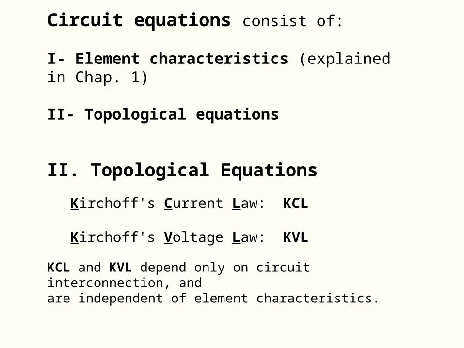
Circuit equations consist of:

I- Element characteristics (explained in Chap. 1)

II- Topological equations

II. Topological Equations

Kirchoff's Current Law: KCL

Kirchoff's Voltage Law: KVL

KCL and KVL depend only on circuit interconnection, and are independent of element characteristics.

Example 2.1

Undirected graph representation

Circuit with 2-terminal elements

1

Directed graph representation (Associated Reference Directions)

Netlist Representation

El. Name n1 n2 Value

I1 3 1 *

R2 1 3 *

R3 1 2 *

R4 1 4 *

R5 3 4 *

R6 2 4 *

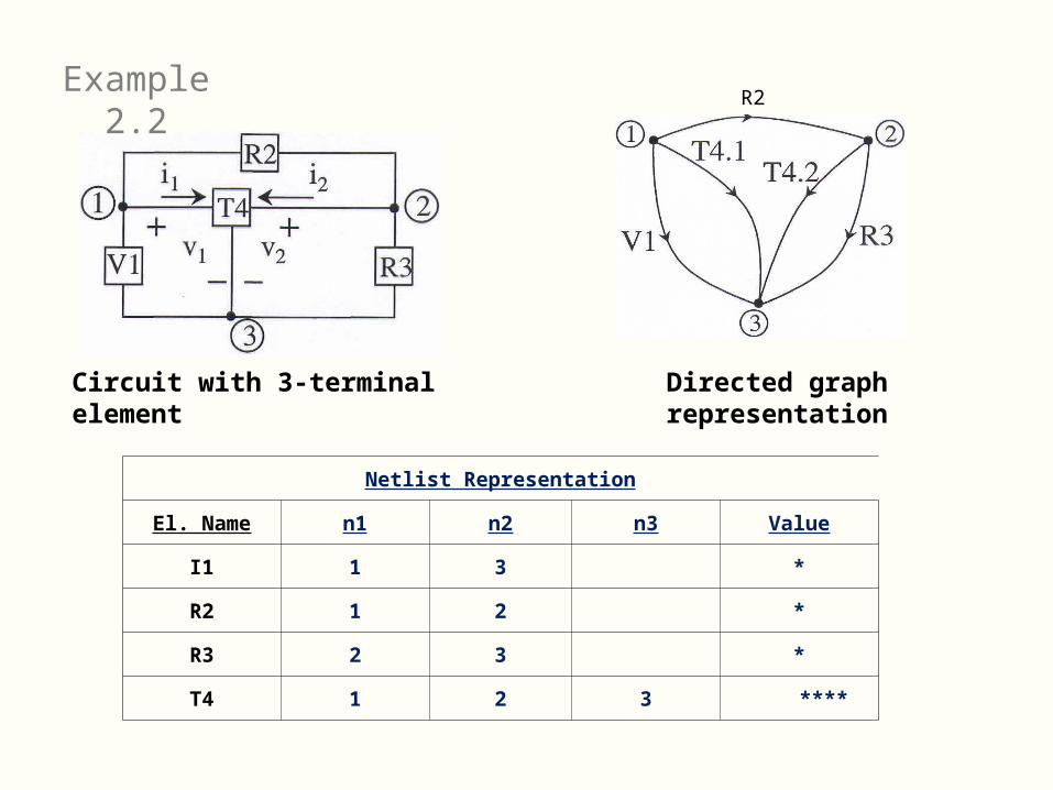
Netlist Representation

El. Name n1 n2 n3 Value

I1 1 3 *

R2 1 2 *

R3 2 3 *

T4 1 2 3 ****

Circuit with 3-terminal element Directed graph representation

Example 2.2 R2

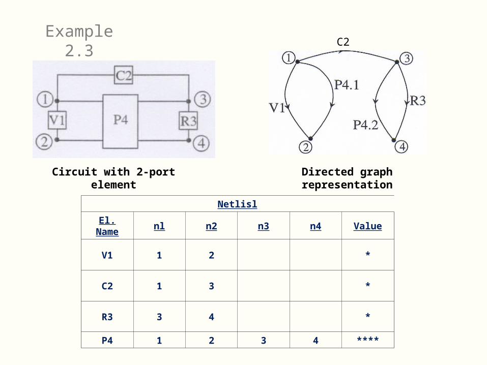
Netlisl

El. Name nl n2 n3 n4 Value

V1 1 2 *

C2 1 3 *

R3 3 4 *

P4 1 2 3 4 ****

Example 2.3

Circuit with 2-port element Directed graph representation

C2

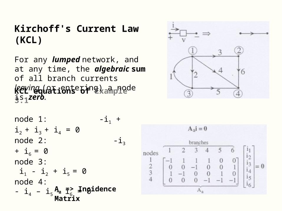
Aa => Incidence Matrix

KCL equations of Example 3.1

node 1: -i1 + i2 + i3 + i4 = 0 node 2: -i3 + i6 = 0node 3: i1 - i2 + i5 = 0 node 4: - i4 – i5 - i6 = 0

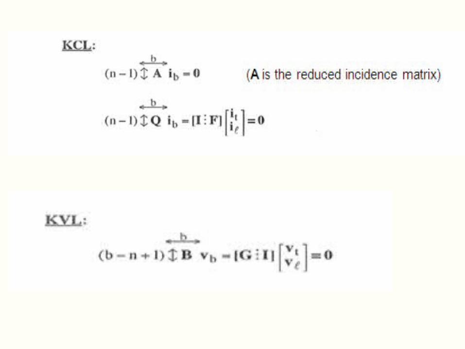
Kirchoff's Current Law (KCL)

For any lumped network, and at any time, the algebraic sum of all branch currents leaving (or entering) a node is zero.

Some properties of Aa:

1. Consists of n rows and b columns; n = # of nodes, b = # of branches

2. Each column contains exactly a "+1" and a "-1“

3. Can be constructed by inspection from the netlist

4. Has rank (n - 1); the n KCL equations are dependent => they add up to zero

5. Can delete any one row (i.e., one KCL equation) to obtain (n - 1) independent KCL equations

KCL Equations: Ai = 0

A is the "reduced" incidence matrix of rank (n - 1)

Loop:

A subgraph L of a graph G is called a loop if:

(1)The subgraph L is connected.

(2) Precisely two branches of L are incident with each node.

Kirchoff's Voltage Law (KVL)

For any lumped network, for any of its loops, and at any time, the algebraic sum of the branch voltages around the loop is zero.

Problem:

How to construct the maximum number of independent loop equations for a given circuit.

For Planar graphs (i.e., graphs that can be drawn in a plane such that no two branches cross at points, other than at nodes)

the number of "windows" give the maximum number of independent loop equations.

However, not all graphs are planar.

In addition, windows cannot be easily recognized from a netlist.

We will thus use the concept of a tree of a graph.

Properties of a tree of a connected graph

• Is a subset of the graph.

• Contains all the nodes.

• Contains no loops.

• Contains (n - 1) branches called tree branches.

• The remaining (b - n + 1) branches are called links or chords.

• For a given graph, there are many different trees (countable in number).

• Each link forms a unique loop with tree branches only (why?).

• The (b - n + 1) loops generated by the links (by taking one link at a time and forming a loop with tree branches only) form a maximum set of independent loop equations. (Why?)

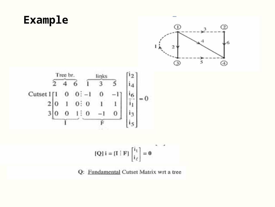
Example KVL wrt tree

KCL Revisited (Cutset Equations)

Cutsets

A set of branches of a connected graph is called a cutset if:

• The removal of all the branches of the set causes the remaining graph to have two separate parts.

• The removal of all but any one of the branches of the set leaves the remaining graph connected.

Example of cutsets

General Form of KCL

• For any lumped network, for any of its cutsets, and at any time, the algebraic sum of all the branch currents traversing the cutset branches is zero

• Each tree branch forms a unique cutset with links only(Why?)

• The (n - 1) KCL equations generated by taking one tree branch at a time and forming a cutset with links only produce a maximum set of independent KCL equations (Why?)

Remarks

• The characteristic equation of a short-circuit is v = 0; i.e. a voltage source with value 0 V

• The characteristic equation of an open-circuit is i = 0; i.e. a current source with value 0 A

• Short-circuits and open circuits can be considered as circuit elements

Example

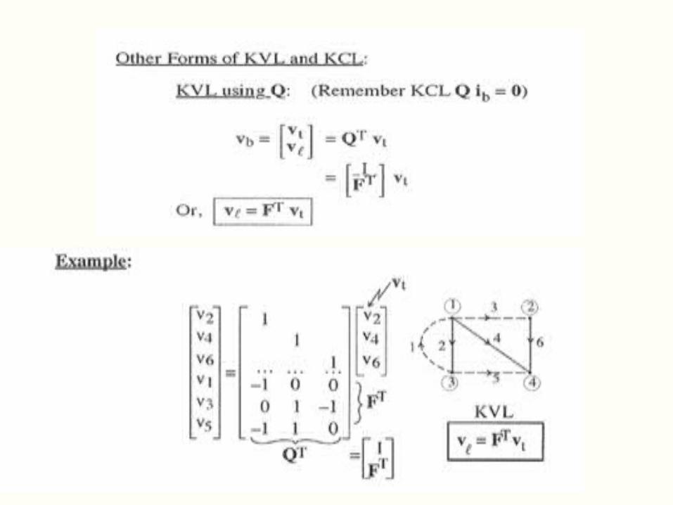
Theorem: QBT= 0 and BQT= 0

When both Q and B are constructed with the same tree and same branch orientations and ordering.

Proof:

Qib = 0, ib = BTil (KCL)Q BTil = 0 for arbitrary il

Therefore, QBT=0

Bvb = 0, vb = QTvt (KVL)BQTvt = 0 for arbitrary vt

Therefore, BQT=0

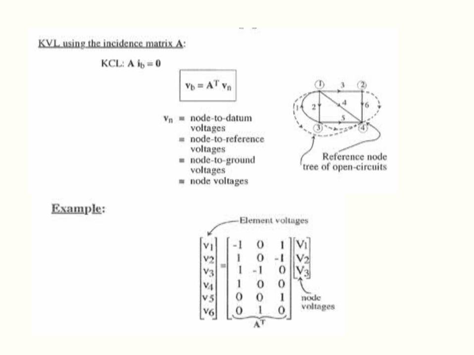
Also: ABT = 0 and BAT = 0

using the same branch orientations and ordering.

Proof:Bvb=0, vb=ATvn (KVL)

BATvn = 0 for arbitrary vn

Therefore BAT = 0

Tellegen’s Theorem

Provided vb and ib follow the associated reference directions, vb satisfies KVL and ib satisfies KCL, independent of element charactersitics.

Proof: vb = QTvt , ib = BTil vbT ib = vt

TQBTil = 0 since QBT=0.

In a lumped circuit, energy is conserved at all times.

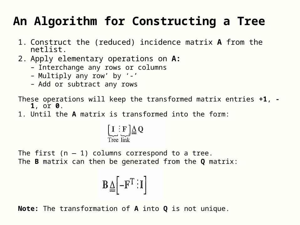
An Algorithm for Constructing a Tree

1. Construct the (reduced) incidence matrix A from the netlist.2. Apply elementary operations on A:

– Interchange any rows or columns– Multiply any row’ by ‘-’ – Add or subtract any rows

These operations will keep the transformed matrix entries +1, -1, or 0.1. Until the A matrix is transformed into the form:

The first (n — 1) columns correspond to a tree.The B matrix can then be generated from the Q matrix:

Note: The transformation of A into Q is not unique.

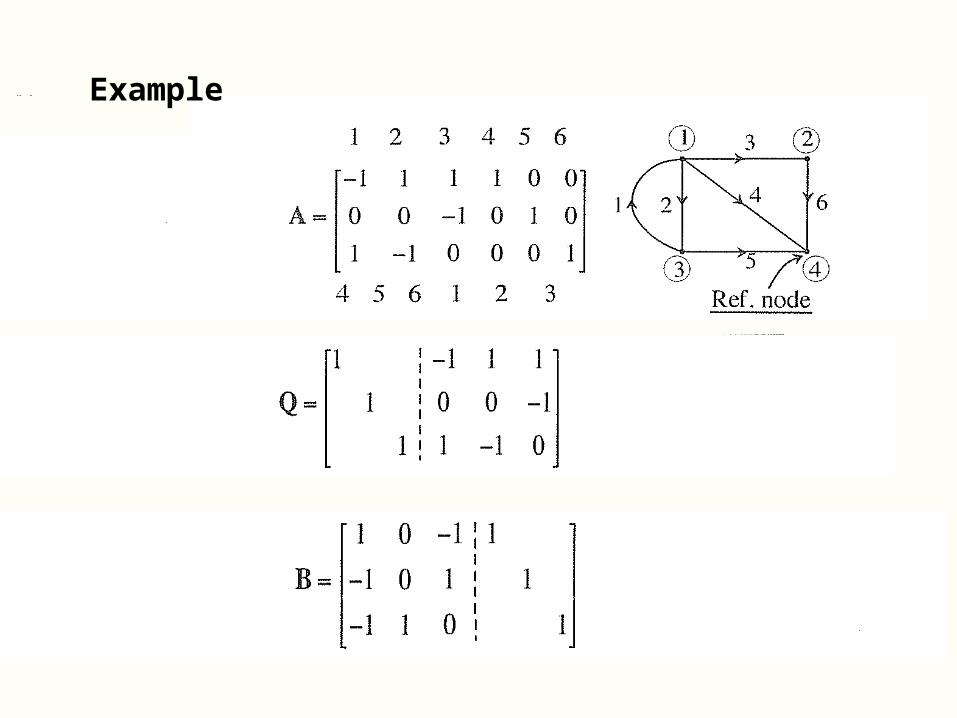
Example

Another way:

Circuit Equations

I. Element characteristics (Linear):

Total number of equations: b-equations in 2b unknowns

For simplicity, consider sinusoidal steady-state analysis:

II. Topological Constraints

(n — 1) equations in b-unknowns

Total number of equations: b-equations in 2b unknowns

In Matrix Form (Tableau Equations): Using Q and B wrt a tree:

Better Ordering

Block Elimination:

OR:

link currents and tree voltages uniquely determine all other variables.

(

Tableau Equations Using the Incidence Matrix

(2b + n - 1) equations in (2b + n - 1) unknowns.There are more equations and more variables and more equations, but there is no need to find a tree

Nodal Analysis

Elements allowed are: conductors (admittances), independent current sources, and voltage- controlled current sources.

Elements not allowed are: independent voltage sources, short-circuits, current- controlled voltage sources, current-controlled

current sources, and voltage-controlled voltage-sources.

Put (2) in (3)

Put (3’) in (1)

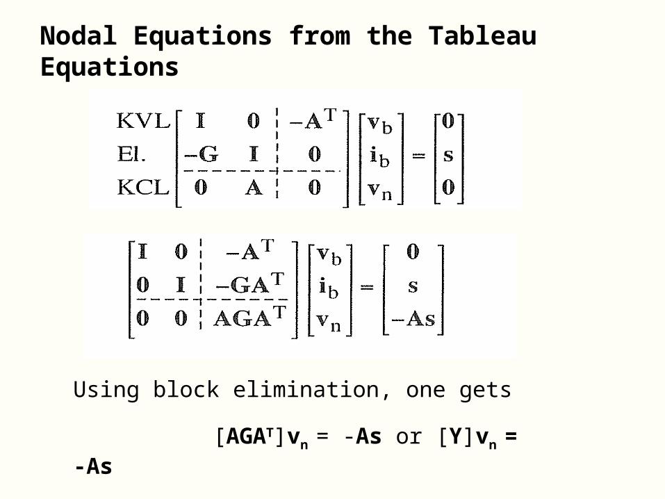
Nodal Equations from the Tableau Equations

Using block elimination, one gets

[AGAT]vn = -As or [Y]vn = -As

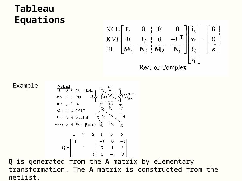
Tableau Equations

Example

Q is generated from the A matrix by elementary transformation. The A matrix is constructed from the netlist.

Nodal Equations

Some Properties of Y:If G is strictly diagonal (no controlled sources) and positive, then:

1- is nonsingular

2- diagonally dominant

3- All diagonal elements are positive, and all off-diagonal elements are negative or zero.

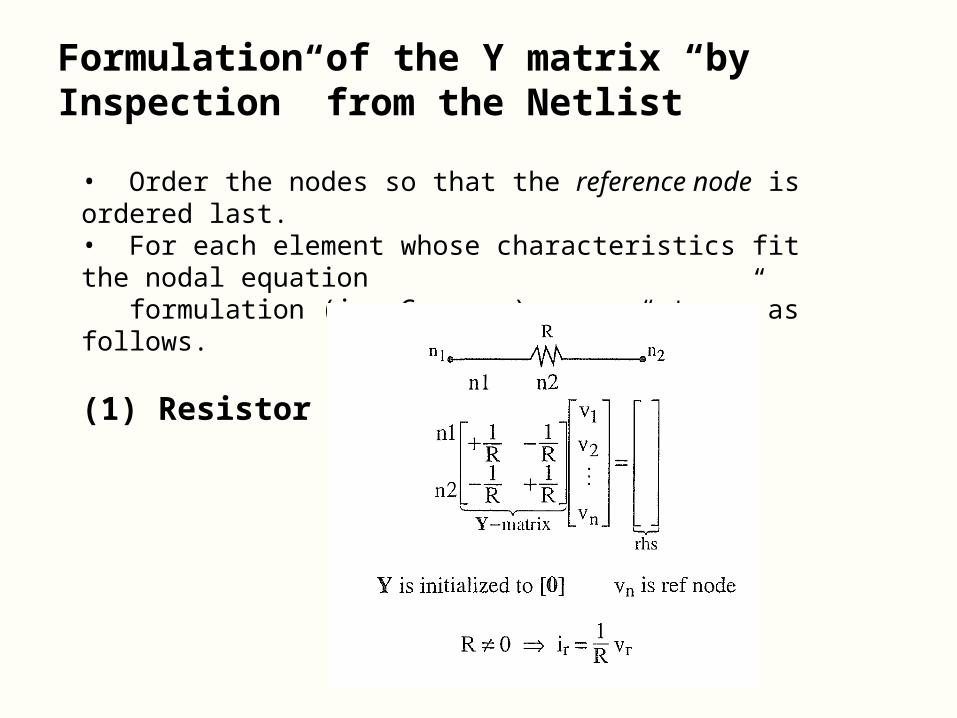
Formulation of the Y matrix “by Inspection” from the Netlist

• Order the nodes so that the reference node is ordered last.• For each element whose characteristics fit the nodal equation formulation (i = G v + s) use a “stamp” as follows.

(1) Resistor

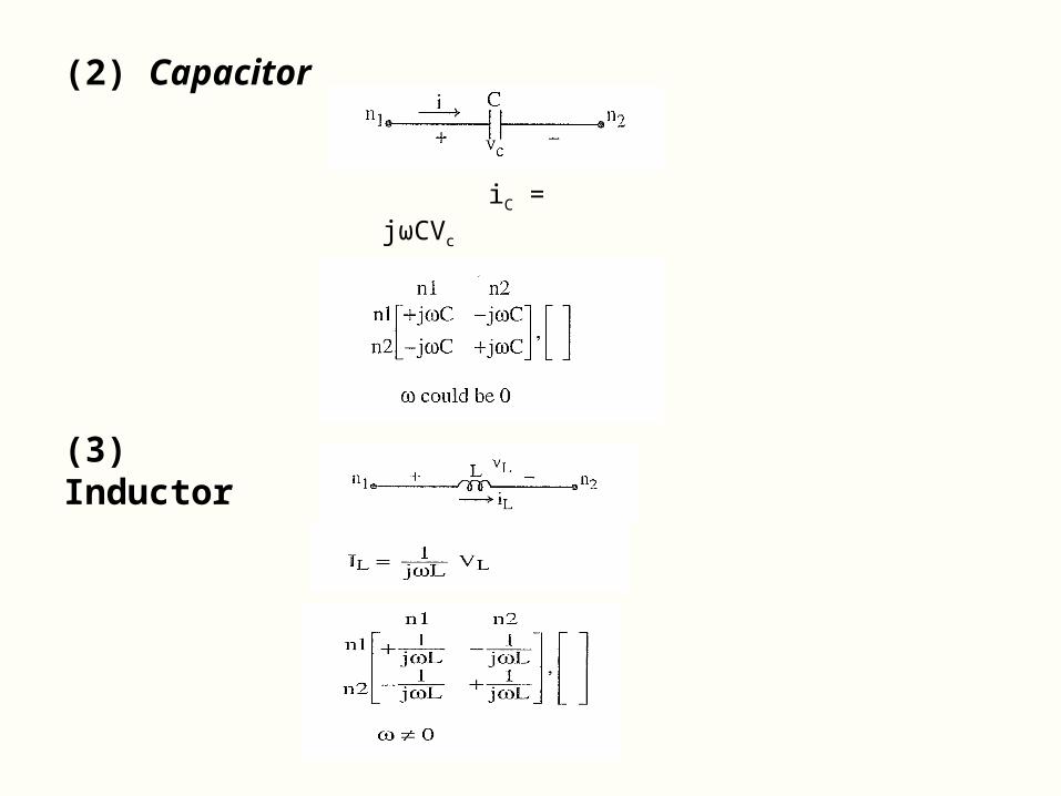
(2) Capacitor

iC = jωCVc

(3) Inductor

(4) Independent Current Source

(5) Voltage-Controlled Current Source

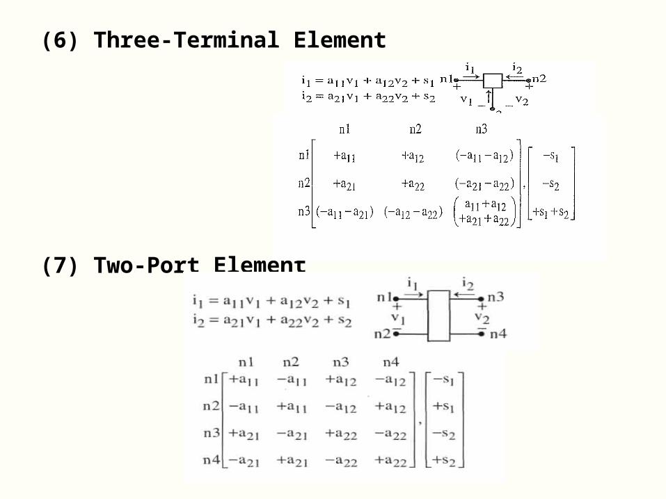
(6) Three-Terminal Element

(7) Two-Port Element

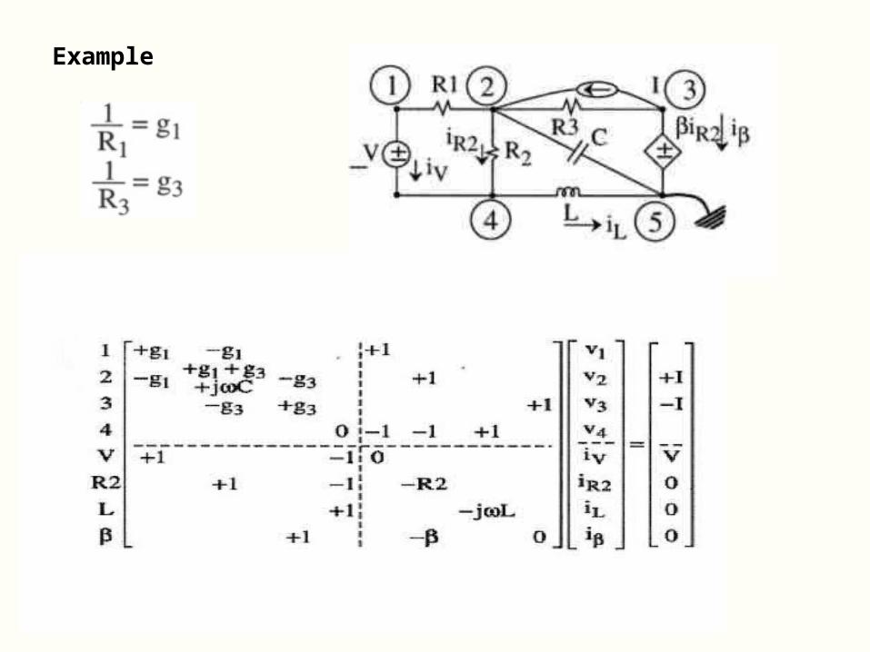
Example

Node 4 is chosen as a reference node.

The “Modified” Nodal Equations

When not all element characteristics fit nodal analysis (e.g. voltage sources)

Assume i1 = G1v1 + H1i2 +s1 (1)

v2 = H2v1 + Z2i2 + s2 (2)

Partition the Incidence Matrix A accordingly

KCL [A1 A2 ] = 0

OR A1i1 + A2i2 = 0 (3)

2

1

i

i

Substitute (4) into (1) and (2):

Put (l') in KCL eqn. (3)

Final equations are (3') and (2')

Derivation of Modified Nodal Equations from the Tableau Equations:

Formulation of Modified Nodal Equations using the “Stamp” Approach

• Partition circuit elements into two sets: El. 1 and El. 2 according to their characteristic equations, as shown above. El. 2 includes voltage sources, short-circuits, inductors, and any element whose current is a declared as a controlling variable

• Declare vn and i2 as the circuit variables

(1) Resistor

* If current in R is not declared a variable

Stamps

(2) Capacitor

(3) Inductor

(4) Independent Current Source

(5) Independent Voltage Source

E

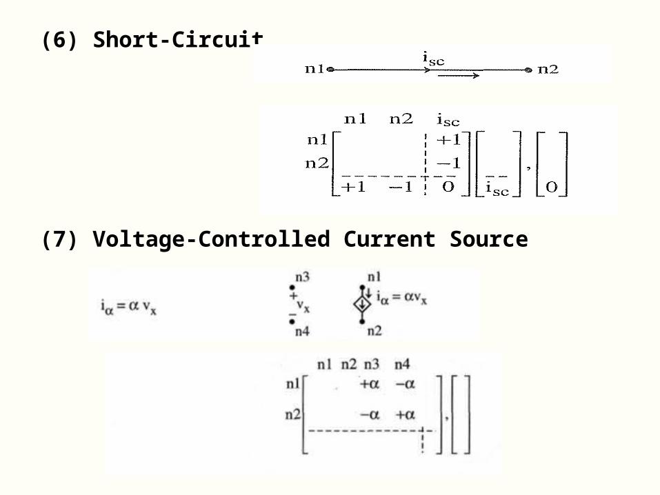
(6) Short-Circuit

(7) Voltage-Controlled Current Source

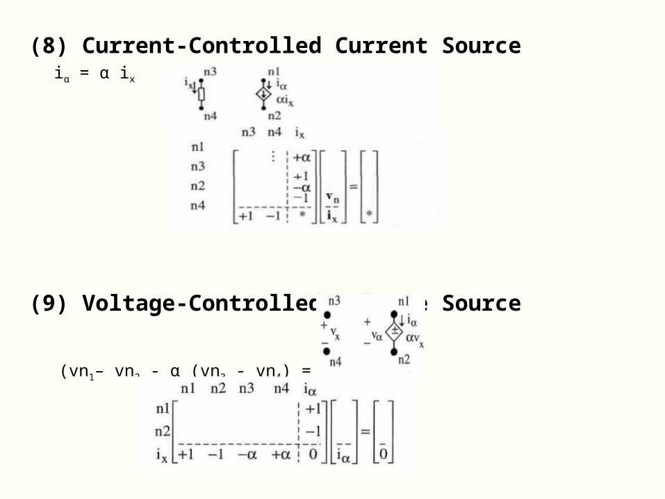
(8) Current-Controlled Current Source iα = α ix

(9) Voltage-Controlled Voltage Source

(vn1– vn2 - α (vn3 - vn4) = 0

(10) Current – Controlled Voltage Source

vnl-vn2- αix = 0

(11) Two-Port (Current-Controlled)Example

V1 = jωL1I1 +jωMI2

V2=jωMI1 +jωLI2

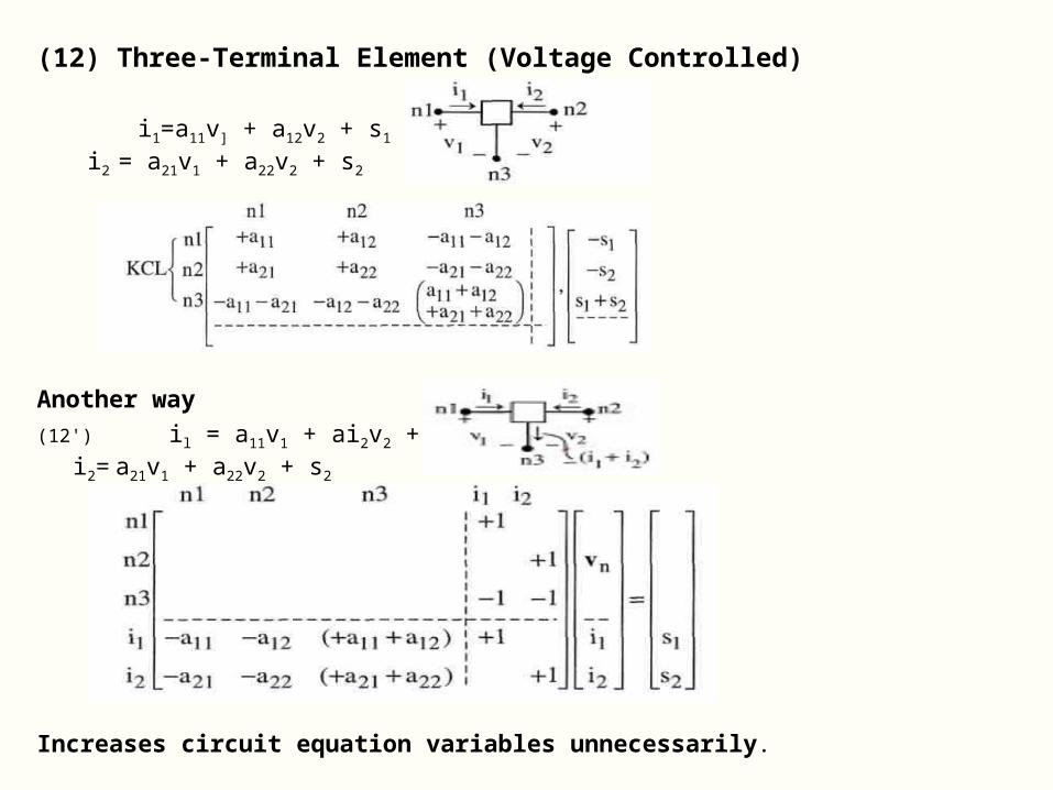
(12) Three-Terminal Element (Voltage Controlled)

i1=a11v] + a12v2 + s1

i2 = a21v1 + a22v2 + s2

Another way

(12') il = a11v1 + ai2v2 + s1

i2= a21v1 + a22v2 + s2

Increases circuit equation variables unnecessarily.

(13) Two-Port (Hybrid Representation) il = allv1 + a12i2 + s1

v2= a2lv1+ a22i2 + s2

vn3-vn4-a21(vnl-vn2)-a22i2 = s2

Another way(13') il = allv1 + a12i2 + s1

v2= a2lv1+ a22i2 + s2

Example

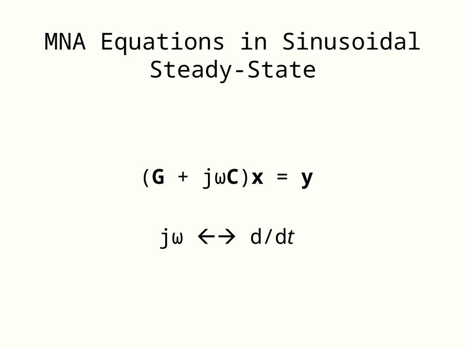
MNA Equations in Sinusoidal Steady-State

(G + jωC)x = y

jω d/dt

Extended Nodal Analysis (ENA)

i1 = G1v1 + H1i2 + N1z + s1

M2v2 = H2v1 + Z2i2 + N2z + s2

z includes variables other than currents and voltages, such as charge, flux, temperature or other parameters, which on turn are functions of voltages and currents.

Extended Nodal Analysis (ENA)

I : -A1T v1 0

I : -A2T v2 0

-G1 I : -H1 -N1 i1 s1

- - - - - :- - - - - - - - - - =

A1: 0 A2 0 vn 0

-H2 M2: 0 -Z2 -N2 i2 s2

z

Extended Nodal Analysis (ENA)

I : -A1T v1 0

I : -A2T v2 0

I : -G1A1T -H1 -N1 i1 s1

- - - - - :- - - - - - - - - - - - - - - - - - - - - - - - =

: A1G1A1T (A1H1+A2) A1N1 vn - A1s1

: (-H2 A1T+M2A2

T) -Z2 -N2 i2 s2

z

Extended Nodal Analysis (ENA)

A1G1A1T (A1H1+A2) A1N1 vn - A1s1

(-H2 A1T+M2A2

T) -Z2 -N2 i2 s2

z