ECE 468: Digital Image Processing

Lecture 15

Prof. Sinisa Todorovic

sinisa@eecs.oregonstate.edu

1

Outline

• Image reconstruction from projections (Textbook 5.11)

• Radon Transform (Textbook 5.11.3)

• Fourier-Slice Theorem (Textbook 5.11.4)

2

Computed Tomography

3

Computed Tomography

4

Radon Transform

A point in the projection

is the ray-sum along

x cos �k + y sin �k = ⇥j

g(⇥j , �k)

5

Two Equivalent Definitions of the Line

y = ax + b

x cos � + y sin � = ⇥

6

continuous space coordinates

Radon Transform

g(⇤, ⇥) =� ⇥

�⇥

� ⇥

�⇥f(x, y)�(x cos ⇥ + y sin ⇥ � ⇤)dxdy

7

continuous space coordinates

Radon Transform

g(⇤, ⇥) =� ⇥

�⇥

� ⇥

�⇥f(x, y)�(x cos ⇥ + y sin ⇥ � ⇤)dxdy

discrete space coordinates

g(⇤, ⇥) =M�1�

x=0

N�1�

y=0

f(x, y)�(x cos ⇥ + y sin ⇥ � ⇤)

7

Example: Radon Transform

f(x, y) =�

A , x2 + y2 � r2

0 , o.w

g(⇢, ✓) =?

8

Example: Radon Transform

g(⇢, ✓) =Z 1

�1

Z 1

�1f(x, y)�(x� ⇢)dxdy

✓ = 0

=Z 1

�1f(⇢, y)dy

9

Example: Radon Transform

g(⇢, ✓) =Z pr2�⇢2

�p

r2�⇢2f(⇢, y)dy

=Z pr2�⇢2

�p

r2�⇢2Ady

10

Properties of the Radon Transform

g(⇢, ✓ + 180

�) =

Z 1

�1

Z 1

�1f(x, y)�(x cos(✓ + 180

�) + y sin(✓ + 180

�)� ⇢) dx dy

=

Z 1

�1

Z 1

�1f(x, y)�(�x cos ✓ � y sin ✓ � ⇢) dx dy

= g(�⇢, ✓)

11

Properties of the Radon Transform

g(⇢, ✓ + 180

�) =

Z 1

�1

Z 1

�1f(x, y)�(x cos(✓ + 180

�) + y sin(✓ + 180

�)� ⇢) dx dy

=

Z 1

�1

Z 1

�1f(x, y)�(�x cos ✓ � y sin ✓ � ⇢) dx dy

= g(�⇢, ✓)

12

Properties of the Radon Transform

g(⇢, ✓ + 180

�) =

Z 1

�1

Z 1

�1f(x, y)�(x cos(✓ + 180

�) + y sin(✓ + 180

�)� ⇢) dx dy

=

Z 1

�1

Z 1

�1f(x, y)�(�x cos ✓ � y sin ✓ � ⇢) dx dy

= g(�⇢, ✓)

13

Sinogram = Image of Radon Transform

14

Properties of Objects from Sinogram

• Sinogram symmetric = Object symmetric

• Sinogram symmetric about image center = Object symmetric and parallel to x and y axes

• Sinogram smooth = Object has uniform intensity

15

Outline

• Fourier-Slice Theorem (Textbook 5.11.4)

16

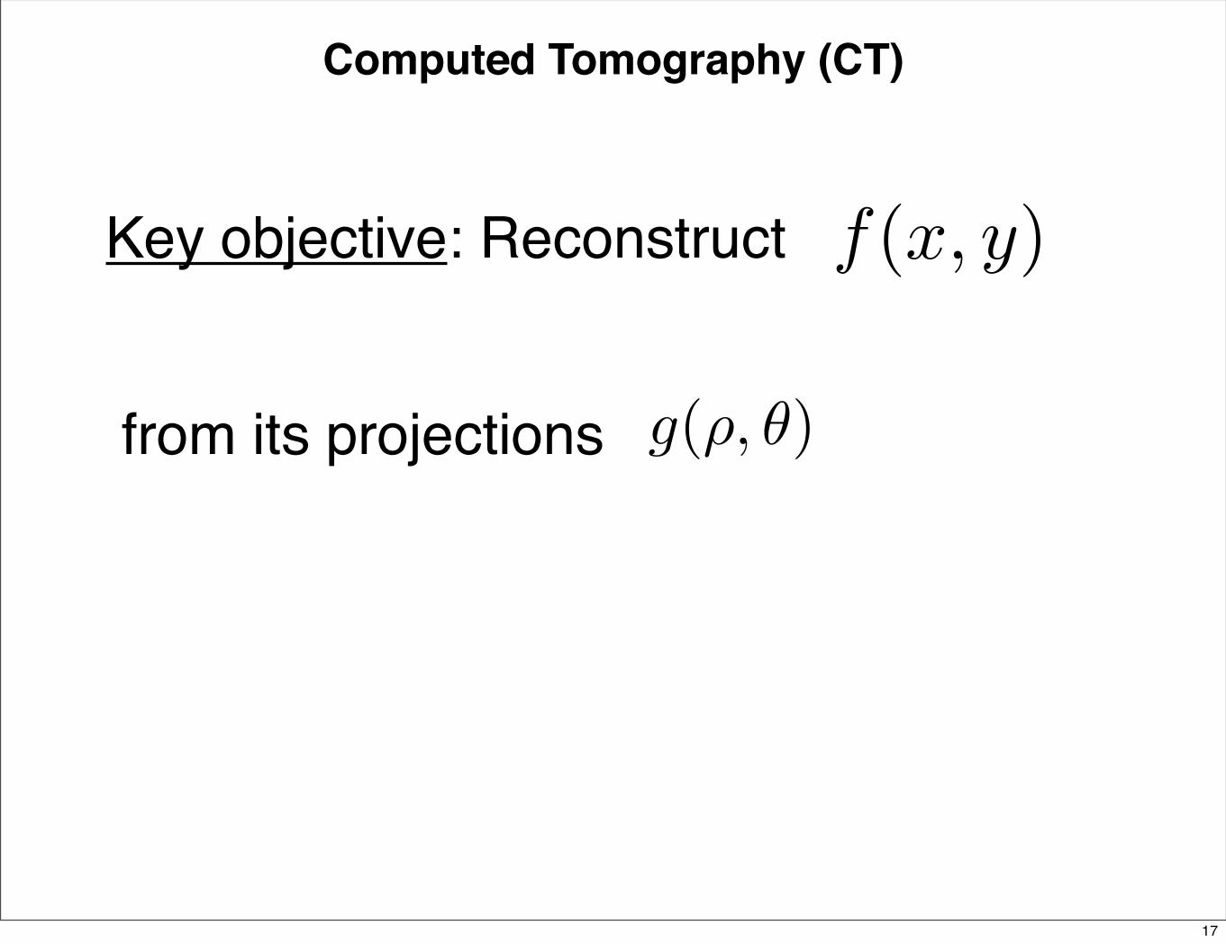
Computed Tomography (CT)

Key objective: Reconstruct

from its projections g(⇢, ✓)

f(x, y)

17

Fourier Slice Theorem

relates

1D Fourier Transform of the projection

with

2D Fourier Transform of the original image

18

1D Fourier Transform of the Projection

G(⇤, �) =� ⇥

�⇥g(⇥, �)e�j2�⇤⇥d⇥

19

1D FT of the Projection -- Properties

G(!, ✓ + 180�) =?

20

1D FT of the Projection -- Properties

G(!, ✓ + 180�) =?

G(!, ✓ + 180�) =Z 1

�1g(⇢, ✓ + 180�)e�j2⇡!⇢d⇢

=Z 1

�1g(�⇢, ✓)e�j2⇡!⇢d⇢

20

1D FT of the Projection -- Properties

G(!, ✓ + 180�) =?

21

1D FT of the Projection -- Properties

G(!, ✓ + 180�) =?

= �Z �1

1g(⇢, ✓)ej2⇡!⇢d⇢

=Z 1

�1g(⇢, ✓)e�j2⇡(�!)⇢d⇢

= G(�!, ✓)

21

Fourier Slice Theorem

G(⇤, �) =� ⇥

�⇥g(⇥, �)e�j2�⇤⇥d⇥

22

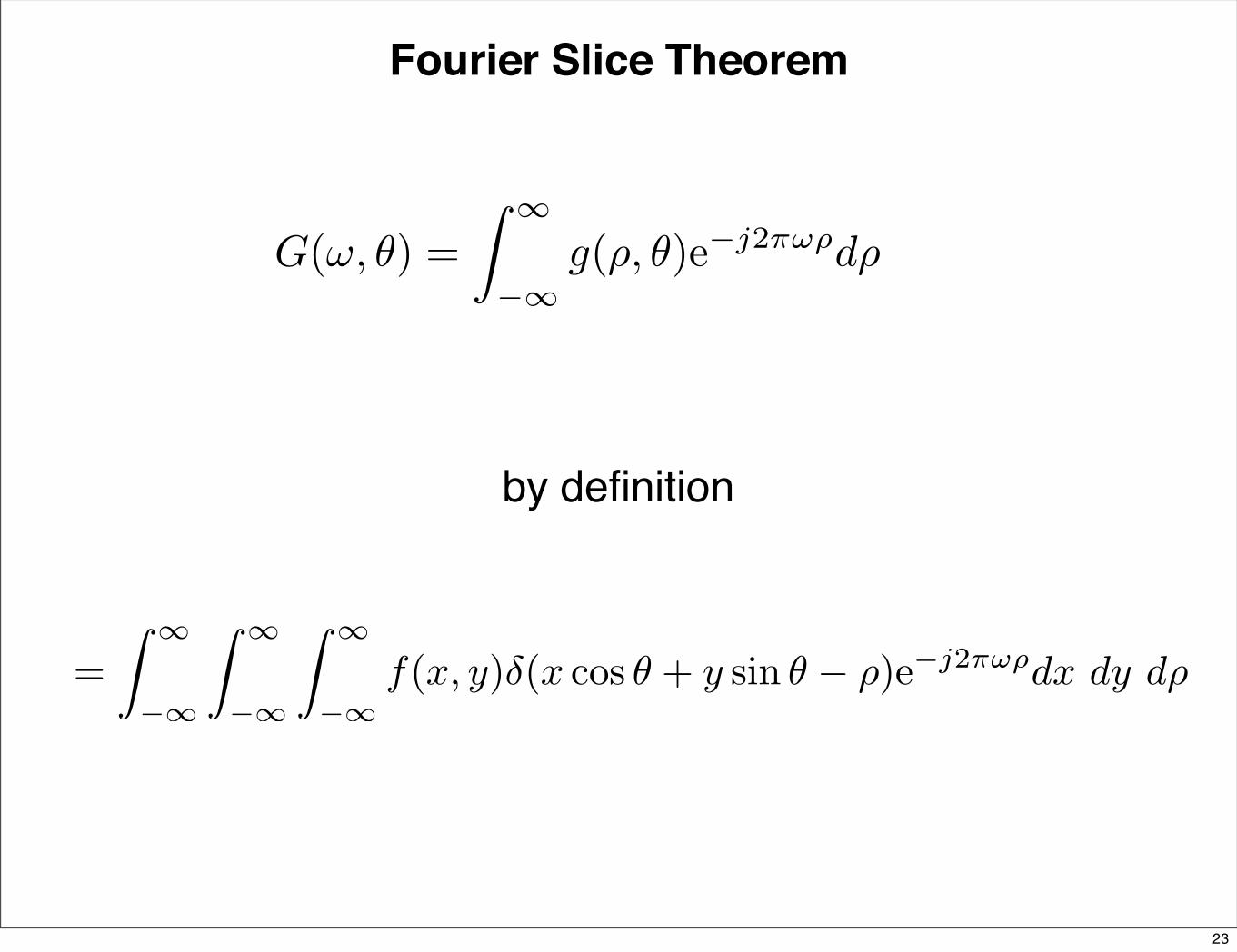
Fourier Slice Theorem

G(⇤, �) =� ⇥

�⇥g(⇥, �)e�j2�⇤⇥d⇥

by definition

G(⌅, ⇥) =� ⇥

�⇥

� ⇥

�⇥

� ⇥

�⇥f(x, y)�(x cos ⇥ + y sin ⇥ � ⇤)e�j2�⇤⇥dx dy d⇤

23

Fourier Slice Theorem

G(⇤, �) =� ⇥

�⇥g(⇥, �)e�j2�⇤⇥d⇥

by definition

24

Fourier Slice Theorem

G(⇤, �) =� ⇥

�⇥g(⇥, �)e�j2�⇤⇥d⇥

by definition

=� ⇥

�⇥

� ⇥

�⇥f(x, y)e�j2⇥⇤(x cos �+y sin �)dx dy

24

Fourier Slice Theorem

G(⇤, �) =� ⇥

�⇥g(⇥, �)e�j2�⇤⇥d⇥

by definition

=� ⇥

�⇥

� ⇥

�⇥f(x, y)e�j2⇥⇤(x cos �+y sin �)dx dy

= F (⇥ cos �,⇥ sin �)24

Fourier Slice Theorem relates

1D Fourier Transform of the projection

with

2D Fourier Transform of the original image

25

Fourier Slice Theorem

1D FT = a slice of 2D FT

26

Reconstruction Using Backprojections

Given , that isg(⇢, ✓) G(!, ✓)

find f(x, y)

27

Reconstruction Using Backprojections

by definition

f(x, y) =� ⇥

�⇥

� ⇥

�⇥F (u, v)ej2�(ux+vy)du dv

28

Reconstruction Using Backprojections

by definition

f(x, y) =� ⇥

�⇥

� ⇥

�⇥F (u, v)ej2�(ux+vy)du dv

u = ⇥ cos �, v = ⇥ sin �, � dudv = ⇥d⇥d�

f(x, y) =� 2⇥

0

� �

0F (⇥ cos �, ⇥ sin �)ej2⇥⇤(x cos �+y sin �)⇥ d⇥ d�

polar coordinates in the frequency domain

28

Reconstruction Using Backprojections

f(x, y) =� 2⇥

0

� �

0F (⇥ cos �, ⇥ sin �)ej2⇥⇤(x cos �+y sin �)⇥ d⇥ d�

29

Reconstruction Using Backprojections

f(x, y) =� 2⇥

0

� �

0F (⇥ cos �, ⇥ sin �)ej2⇥⇤(x cos �+y sin �)⇥ d⇥ d�

f(x, y) =� 2⇥

0

� �

0G(⇥, �)ej2⇥⇤(x cos �+y sin �)⇥ d⇥ d�

by Fourier Slice Theorem

29

Reconstruction Using Backprojections

f(x, y) =� 2⇥

0

� �

0G(⇥, �)ej2⇥⇤(x cos �+y sin �)⇥ d⇥ d�

30

Reconstruction Using Backprojections

f(x, y) =� 2⇥

0

� �

0G(⇥, �)ej2⇥⇤(x cos �+y sin �)⇥ d⇥ d�

f(x, y) =� ⇥

0

� �

0|⇥|G(⇥, �)ej2⇥⇤(x cos �+y sin �) d⇥ d�

G(⇥, � + 180�) = G(�⇥, �)

30

Reconstruction Using Backprojections

31

Reconstruction Using Backprojections

f(x, y) =⇤ ⇥

0

�⇤ �

0|⇥|G(⇥, �)ej2⇥⌅⇤ d⇥

⇥

⇤=x cos �+y sin �

d�

31

Reconstruction Using Backprojections

f(x, y) =⇤ ⇥

0

�⇤ �

0|⇥|G(⇥, �)ej2⇥⌅⇤ d⇥

⇥

⇤=x cos �+y sin �

d�

1D filtering

31

Box + Ramp Filter

32

Algorithm for Filtered Backprojection

1. Given projections g(ρ,θ) obtained at each fixed angle θ

2. Compute G(ω,θ) = 1D Fourier Transform of each projection g(ρ,θ)

3. Multiply G(ω,θ) by the filter function |ω| modified by Hamming window

4. Compute the inverse of the results from 3.

5. Integrate (sum) over θ all results from 4.

33

Examples

rampfilter

windowedramp filter

rampfilter

windowedramp filter

zoom

34