Embed Size (px)
Citation preview
EBSeq: An R package for differential expression analysis using
RNA-seq data
Ning Leng, John Dawson, and Christina Kendziorski
October 13, 2014
Contents
1 Introduction 2
2 Citing this software 2
3 The Model 23.1 Two conditions . . . . . . . . . . . . . . . . . . . . . . . . . . . . . . . . . . . . . . . . . . . . 23.2 More than two conditions . . . . . . . . . . . . . . . . . . . . . . . . . . . . . . . . . . . . . . 43.3 Getting a false discovery rate (FDR) controlled list of genes or isoforms . . . . . . . . . . . . 4
4 Quick Start 54.1 Gene level DE analysis (two conditions) . . . . . . . . . . . . . . . . . . . . . . . . . . . . . . 5
4.1.1 Required input . . . . . . . . . . . . . . . . . . . . . . . . . . . . . . . . . . . . . . . . 54.1.2 Library size factor . . . . . . . . . . . . . . . . . . . . . . . . . . . . . . . . . . . . . . 54.1.3 Running EBSeq on gene expression estimates . . . . . . . . . . . . . . . . . . . . . . . 5
4.2 Isoform level DE analysis (two conditions) . . . . . . . . . . . . . . . . . . . . . . . . . . . . . 64.2.1 Required inputs . . . . . . . . . . . . . . . . . . . . . . . . . . . . . . . . . . . . . . . 64.2.2 Library size factor . . . . . . . . . . . . . . . . . . . . . . . . . . . . . . . . . . . . . . 74.2.3 The Ig vector . . . . . . . . . . . . . . . . . . . . . . . . . . . . . . . . . . . . . . . . . 74.2.4 Running EBSeq on isoform expression estimates . . . . . . . . . . . . . . . . . . . . . 7
4.3 Gene level DE analysis (more than two conditions) . . . . . . . . . . . . . . . . . . . . . . . . 84.4 Isoform level DE analysis (more than two conditions) . . . . . . . . . . . . . . . . . . . . . . . 10
5 More detailed examples 135.1 Gene level DE analysis (two conditions) . . . . . . . . . . . . . . . . . . . . . . . . . . . . . . 13
5.1.1 Running EBSeq on simulated gene expression estimates . . . . . . . . . . . . . . . . . 135.1.2 Calculating FC . . . . . . . . . . . . . . . . . . . . . . . . . . . . . . . . . . . . . . . . 135.1.3 Checking convergence . . . . . . . . . . . . . . . . . . . . . . . . . . . . . . . . . . . . 145.1.4 Checking the model fit and other diagnostics . . . . . . . . . . . . . . . . . . . . . . . 15
5.2 Isoform level DE analysis (two conditions) . . . . . . . . . . . . . . . . . . . . . . . . . . . . . 175.2.1 The Ig vector . . . . . . . . . . . . . . . . . . . . . . . . . . . . . . . . . . . . . . . . . 175.2.2 Using mappability ambiguity clusters instead of the Ig vector when the gene-isoform
relationship is unknown . . . . . . . . . . . . . . . . . . . . . . . . . . . . . . . . . . . 185.2.3 Running EBSeq on simulated isoform expression estimates . . . . . . . . . . . . . . . 185.2.4 Checking convergence . . . . . . . . . . . . . . . . . . . . . . . . . . . . . . . . . . . . 195.2.5 Checking the model fit and other diagnostics . . . . . . . . . . . . . . . . . . . . . . . 19
5.3 Gene level DE analysis (more than two conditions) . . . . . . . . . . . . . . . . . . . . . . . . 245.4 Isoform level DE analysis (more than two conditions) . . . . . . . . . . . . . . . . . . . . . . . 29
1
5.5 Working without replicates . . . . . . . . . . . . . . . . . . . . . . . . . . . . . . . . . . . . . 345.5.1 Gene counts with two conditions . . . . . . . . . . . . . . . . . . . . . . . . . . . . . . 345.5.2 Isoform counts with two conditions . . . . . . . . . . . . . . . . . . . . . . . . . . . . . 345.5.3 Gene counts with more than two conditions . . . . . . . . . . . . . . . . . . . . . . . . 355.5.4 Isoform counts with more than two conditions . . . . . . . . . . . . . . . . . . . . . . 35
6 EBSeq pipelines and extensions 366.1 RSEM-EBSeq pipeline: from raw reads to differential expression analysis results . . . . . . . 366.2 EBSeq interface: A user-friendly graphical interface for differetial expression analysis . . . . . 366.3 EBSeq Galaxy tool shed . . . . . . . . . . . . . . . . . . . . . . . . . . . . . . . . . . . . . . . 36
7 Acknowledgment 36
8 News 37
1 Introduction
EBSeq may be used to identify differentially expressed (DE) genes and isoforms in an RNA-Seq experiment.As detailed in Leng et al., 2013 [3], EBSeq is an empirical Bayesian approach that models a number offeatures observed in RNA-seq data. Importantly, for isoform level inference, EBSeq directly accommodatesisoform expression estimation uncertainty by modeling the differential variability observed in distinct groupsof isoforms. Consider Figure 1, where we have plotted variance against mean for all isoforms using RNA-Seqexpression data from Leng et al., 2013 [3]. Also shown is the fit within three sub-groups of isoforms definedby the number of constituent isoforms of the parent gene. An isoform of gene g is assigned to the Ig = kgroup, where k = 1, 2, 3, if the total number of isoforms from gene g is k (the Ig = 3 group contains allisoforms from genes having 3 or more isoforms). As shown in Figure 1, there is decreased variability in theIg = 1 group, but increased variability in the others, due to the relative increase in uncertainty inherent inestimating isoform expression when multiple isoforms of a given gene are present. If this structure is notaccommodated, there is reduced power for identifying isoforms in the Ig = 1 group (since the true variancesin that group are lower, on average, than that derived from the full collection of isoforms) as well as increasedfalse discoveries in the Ig = 2 and Ig = 3 groups (since the true variances are higher, on average, than thosederived from the full collection). EBSeq directly models differential variability as a function of Ig providinga powerful approach for isoform level inference. As shown in Leng et al., 2013 [3], the model is also usefulfor identifying DE genes. We will briefly detail the model in Section 3 and then describe the flow of analysisin Section 4 for both isoform and gene-level inference.
2 Citing this software
Please cite the following article when reporting results from the software.Leng, N., J.A. Dawson, J.A. Thomson, V. Ruotti, A.I. Rissman, B.M.G. Smits, J.D. Haag, M.N. Gould,R.M. Stewart, and C. Kendziorski. EBSeq: An empirical Bayes hierarchical model for inference in RNA-seqexperiments, Bioinformatics, 2013.
3 The Model
3.1 Two conditions
We let XC1gi = Xgi,1, Xgi,2, ..., Xgi,S1
denote data from condition 1 and XC2gi = Xgi,(S1+1), Xgi,(S1+2), ..., Xgi,S
data from condition 2. We assume that counts within condition C are distributed as Negative Binomial:
2
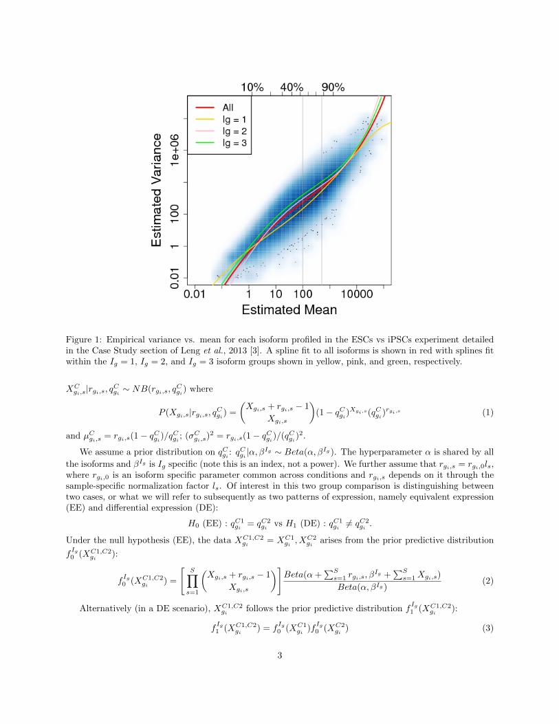
Figure 1: Empirical variance vs. mean for each isoform profiled in the ESCs vs iPSCs experiment detailedin the Case Study section of Leng et al., 2013 [3]. A spline fit to all isoforms is shown in red with splines fitwithin the Ig = 1, Ig = 2, and Ig = 3 isoform groups shown in yellow, pink, and green, respectively.
XCgi,s|rgi,s, q
Cgi ∼ NB(rgi,s, q
Cgi) where
P (Xgi,s|rgi,s, qCgi) =
(Xgi,s + rgi,s − 1
Xgi,s
)(1− qCgi)
Xgi,s(qCgi)rgi,s (1)
and µCgi,s = rgi,s(1− qCgi)/q
Cgi ; (σC
gi,s)2 = rgi,s(1− qCgi)/(q
Cgi)
2.
We assume a prior distribution on qCgi : qCgi |α, β
Ig ∼ Beta(α, βIg ). The hyperparameter α is shared by all
the isoforms and βIg is Ig specific (note this is an index, not a power). We further assume that rgi,s = rgi,0ls,where rgi,0 is an isoform specific parameter common across conditions and rgi,s depends on it through thesample-specific normalization factor ls. Of interest in this two group comparison is distinguishing betweentwo cases, or what we will refer to subsequently as two patterns of expression, namely equivalent expression(EE) and differential expression (DE):
H0 (EE) : qC1gi = qC2
gi vs H1 (DE) : qC1gi 6= qC2
gi .
Under the null hypothesis (EE), the data XC1,C2gi = XC1
gi , XC2gi arises from the prior predictive distribution
fIg0 (XC1,C2
gi ):
fIg0 (XC1,C2
gi ) =
[S∏
s=1
(Xgi,s + rgi,s − 1
Xgi,s
)]Beta(α+
∑Ss=1 rgi,s, β
Ig +∑S
s=1Xgi,s)
Beta(α, βIg )(2)
Alternatively (in a DE scenario), XC1,C2gi follows the prior predictive distribution f
Ig1 (XC1,C2
gi ):
fIg1 (XC1,C2
gi ) = fIg0 (XC1
gi )fIg0 (XC2
gi ) (3)
3
Let the latent variable Zgi be defined so that Zgi = 1 indicates that isoform gi is DE and Zgi = 0 indicatesisoform gi is EE, and Zgi ∼ Bernoulli(p). Then, the marginal distribution of XC1,C2
gi and Zgi is:
(1− p)f Ig0 (XC1,C2gi ) + pf
Ig1 (XC1,C2
gi ) (4)
The posterior probability of being DE at isoform gi is obtained by Bayes’ rule:
pfIg1 (XC1,C2
gi )
(1− p)f Ig0 (XC1,C2gi ) + pf
Ig1 (XC1,C2
gi )(5)
3.2 More than two conditions
EBSeq naturally accommodates multiple condition comparisons. For example, in a study with 3 conditions,there are K=5 possible expression patterns (P1,...,P5), or ways in which latent levels of expression may varyacross conditions:
P1: qC1gi = qC2
gi = qC3gi
P2: qC1gi = qC2
gi 6= qC3gi
P3: qC1gi = qC3
gi 6= qC2gi
P4: qC1gi 6= qC2
gi = qC3gi
P5: qC1gi 6= qC2
gi 6= qC3gi and qC1
gi 6= qC3gi
The prior predictive distributions for these are given, respectively, by:
gIg1 (XC1,C2,C3
gi ) = fIg0 (XC1,C2,C3
gi )
gIg2 (XC1,C2,C3
gi ) = fIg0 (XC1,C2
gi )fIg0 (XC3
gi )
gIg3 (XC1,C2,C3
gi ) = fIg0 (XC1,C3
gi )fIg0 (XC2
gi )
gIg4 (XC1,C2,C3
gi ) = fIg0 (XC1
gi )fIg0 (XC2,C3
gi )
gIg5 (XC1,C2,C3
gi ) = fIg0 (XC1
gi )fIg0 (XC2
gi )fIg0 (XC3
gi )
where fIg0 is the same as in equation 2. Then the marginal distribution in equation 4 becomes:
5∑k=1
pkgIgk (XC1,C2,C3
gi ) (6)
where∑5
k=1 pk = 1. Thus, the posterior probability of isoform gi coming from pattern K is readily obtainedby:
pKgIgK (XC1,C2,C3
gi )∑5k=1 pkg
Igk (XC1,C2,C3
gi )(7)
3.3 Getting a false discovery rate (FDR) controlled list of genes or isoforms
To obtain a list of DE genes with false discovery rate (FDR) controlled at α in an experiment comparing twobiological conditions, the genes with posterior probability of being DE (PPDE) greater than 1 - α should beused. For example, the genes with PPDE>=0.95 make up the list of DE genes with target FDR controlledat 5%. With more than two biological conditions, there are multiple DE patterns (see Section 3.2). Toobtain a list of genes in a specific DE pattern with target FDR α, a user should take the genes with posteriorprobability of being in that pattern greater than 1 - α. Isoform-based lists are obtained in the same way.
4
4 Quick Start
Before analysis can proceed, the EBSeq package must be loaded into the working space:
> library(EBSeq)
4.1 Gene level DE analysis (two conditions)
4.1.1 Required input
Data: The object Data should be a G− by − S matrix containing the expression values for each gene andeach sample, where G is the number of genes and S is the number of samples. These values should exhibitraw counts, without normalization across samples. Counts of this nature may be obtained from RSEM [4],Cufflinks [6], or a similar approach.
Conditions: The object Conditions should be a Factor vector of length S that indicates to whichcondition each sample belongs. For example, if there are two conditions and three samples in each, S = 6and Conditions may be given byas.factor(c("C1","C1","C1","C2","C2","C2"))
The object GeneMat is a simulated data matrix containing 1,000 rows of genes and 10 columns of samples.The genes are named Gene_1, Gene_2 ...
> data(GeneMat)
> str(GeneMat)
num [1:1000, 1:10] 1879 24 3291 97 485 ...
- attr(*, "dimnames")=List of 2
..$ : chr [1:1000] "Gene_1" "Gene_2" "Gene_3" "Gene_4" ...
..$ : NULL
4.1.2 Library size factor
As detailed in Section 3, EBSeq requires the library size factor ls for each sample s. Here, ls may be obtainedvia the function MedianNorm, which reproduces the median normalization approach in DESeq [1].
> Sizes=MedianNorm(GeneMat)
If quantile normalization is preferred, ls may be obtained via the function QuantileNorm. (e.g. QuantileNorm(GeneMat,.75)for Upper-Quantile Normalization in [2])
4.1.3 Running EBSeq on gene expression estimates
The function EBTest is used to detect DE genes. For gene-level data, we don’t need to specify the parameterNgVector since there are no differences in Ig structure among the different genes. Here, we simulated thefirst five samples to be in condition 1 and the other five in condition 2, so define:
Conditions=as.factor(rep(c("C1","C2"),each=5))
sizeFactors is used to define the library size factor of each sample. It could be obtained by summing upthe total number of reads within each sample, Median Normalization [1], scaling normalization [5], Upper-Quantile Normalization [2], or some other such approach. These in hand, we run the EM algorithm, settingthe number of iterations to five via maxround=5 for demonstration purposes. However, we note that inpractice, additional iterations are usually required. Convergence should always be checked (see Section 5.1.3for details). Please note this may take several minutes:
> EBOut=EBTest(Data=GeneMat,
+ Conditions=as.factor(rep(c("C1","C2"),each=5)),sizeFactors=Sizes, maxround=5)
5
Removing transcripts with 75 th quantile < = 10
950 transcripts will be tested
The posterior probabilities of being DE are obtained as follows, where PP is a matrix containing the posteriorprobabilities of being EE or DE for each of the 1,000 simulated genes:
> PP=GetPPMat(EBOut)
> str(PP)
num [1:950, 1:2] 0 0 0 0 0 ...
- attr(*, "dimnames")=List of 2
..$ : chr [1:950] "Gene_1" "Gene_2" "Gene_3" "Gene_4" ...
..$ : chr [1:2] "PPEE" "PPDE"
> head(PP)
PPEE PPDE
Gene_1 0.000000e+00 1
Gene_2 0.000000e+00 1
Gene_3 0.000000e+00 1
Gene_4 0.000000e+00 1
Gene_5 0.000000e+00 1
Gene_6 4.645857e-10 1
The matrix PP contains two columns PPEE and PPDE, corresponding to the posterior probabilities of beingEE or DE for each gene. PP may be used to form an FDR-controlled list of DE genes with a target FDR of0.05 as follows:
> DEfound=rownames(PP)[which(PP[,"PPDE"]>=.95)]
> str(DEfound)
chr [1:97] "Gene_1" "Gene_2" "Gene_3" "Gene_4" "Gene_5" ...
EBSeq found 98 DE genes in total with target FDR 0.05.
4.2 Isoform level DE analysis (two conditions)
4.2.1 Required inputs
Data: The object Data should be a I − by − S matrix containing the expression values for each isoformand each sample, where I is the number of isoforms and S is the number of sample. As in the gene-levelanalysis, these values should exhibit raw data, without normalization across samples.
Conditions: The object Conditions should be a vector with length S to indicate the condition of eachsample.
IsoformNames: The object IsoformNames should be a vector with length I to indicate the isoform names.
IsosGeneNames: The object IsosGeneNames should be a vector with length I to indicate the gene nameof each isoform. (in the same order as IsoformNames.)
IsoList contains 1,200 simulated isoforms. In which IsoList$IsoMat is a data matrix containing 1,200 rowsof isoforms and 10 columns of samples; IsoList$IsoNames contains the isoform names; IsoList$IsosGeneNamescontains the names of the genes the isoforms belong to.
6
> data(IsoList)
> str(IsoList)
List of 3
$ IsoMat : num [1:1200, 1:10] 176 789 1300 474 1061 ...
..- attr(*, "dimnames")=List of 2
.. ..$ : chr [1:1200] "Iso_1_1" "Iso_1_2" "Iso_1_3" "Iso_1_4" ...
.. ..$ : NULL
$ IsoNames : chr [1:1200] "Iso_1_1" "Iso_1_2" "Iso_1_3" "Iso_1_4" ...
$ IsosGeneNames: chr [1:1200] "Gene_1" "Gene_2" "Gene_3" "Gene_4" ...
> IsoMat=IsoList$IsoMat
> str(IsoMat)
num [1:1200, 1:10] 176 789 1300 474 1061 ...
- attr(*, "dimnames")=List of 2
..$ : chr [1:1200] "Iso_1_1" "Iso_1_2" "Iso_1_3" "Iso_1_4" ...
..$ : NULL
> IsoNames=IsoList$IsoNames
> IsosGeneNames=IsoList$IsosGeneNames
4.2.2 Library size factor
Similar to the gene-level analysis presented above, we may obtain the isoform-level library size factors viaMedianNorm:
> IsoSizes=MedianNorm(IsoMat)
4.2.3 The Ig vector
While working on isoform level data, EBSeq fits different prior parameters for different uncertainty groups(defined as Ig groups). The default setting to define the uncertainty groups consists of using the number ofisoforms the host gene contains (Ng) for each isoform. The default settings will provide three uncertaintygroups:
Ig = 1 group: Isoforms with Ng = 1;Ig = 2 group: Isoforms with Ng = 2;Ig = 3 group: Isoforms with Ng ≥ 3.The Ng and Ig group assignment can be obtained using the function GetNg. The required inputs of GetNg
are the isoform names (IsoformNames) and their corresponding gene names (IsosGeneNames).
> NgList=GetNg(IsoNames, IsosGeneNames)
> IsoNgTrun=NgList$IsoformNgTrun
> IsoNgTrun[c(1:3,201:203,601:603)]
Iso_1_1 Iso_1_2 Iso_1_3 Iso_2_1 Iso_2_2 Iso_2_3 Iso_3_1 Iso_3_2 Iso_3_3
1 1 1 2 2 2 3 3 3
More details could be found in Section 5.2.
4.2.4 Running EBSeq on isoform expression estimates
The EBTest function is also used to run EBSeq for two condition comparisons on isoform-level data. Belowwe use 5 iterations to demonstrate. However, as in the gene level analysis, we advise that additional iterationswill likely be required in practice (see Section 5.2.4 for details).
7
> IsoEBOut=EBTest(Data=IsoMat, NgVector=IsoNgTrun,
+ Conditions=as.factor(rep(c("C1","C2"),each=5)),sizeFactors=IsoSizes, maxround=5)
Removing transcripts with 75 th quantile < = 10
1102 transcripts will be tested
> IsoPP=GetPPMat(IsoEBOut)
> str(IsoPP)
num [1:1102, 1:2] 0 0 0 0 0 ...
- attr(*, "dimnames")=List of 2
..$ : chr [1:1102] "Iso_1_1" "Iso_1_2" "Iso_1_3" "Iso_1_4" ...
..$ : chr [1:2] "PPEE" "PPDE"
> head(IsoPP)
PPEE PPDE
Iso_1_1 0 1
Iso_1_2 0 1
Iso_1_3 0 1
Iso_1_4 0 1
Iso_1_5 0 1
Iso_1_6 0 1
> IsoDE=rownames(IsoPP)[which(IsoPP[,"PPDE"]>=.95)]
> str(IsoDE)
chr [1:106] "Iso_1_1" "Iso_1_2" "Iso_1_3" "Iso_1_4" "Iso_1_5" ...
We see that EBSeq found 105 DE isoforms at the target FDR of 0.05.
4.3 Gene level DE analysis (more than two conditions)
The object MultiGeneMat is a matrix containing 500 simulated genes with 6 samples: the first two samplesare from condition 1; the second and the third sample are from condition 2; the last two samples are fromcondition 3.
> data(MultiGeneMat)
> str(MultiGeneMat)
num [1:500, 1:6] 411 268 768 1853 878 ...
- attr(*, "dimnames")=List of 2
..$ : chr [1:500] "Gene_1" "Gene_3" "Gene_5" "Gene_7" ...
..$ : NULL
In analysis where the data are spread over more than two conditions, the set of possible patterns for each geneis more complicated than simply EE and DE. As noted in Section 3, when we have 3 conditions, there are5 expression patterns to consider. In the simulated data, we have 6 samples, 2 in each of 3 conditions. Thefunction GetPatterns allows the user to generate all possible patterns given the conditions. For example:
> Conditions=c("C1","C1","C2","C2","C3","C3")
> PosParti=GetPatterns(Conditions)
> PosParti
8
C1 C2 C3
Pattern1 1 1 1
Pattern2 1 1 2
Pattern3 1 2 1
Pattern4 1 2 2
Pattern5 1 2 3
where the first row means all three conditions have the same latent mean expression level; the second rowmeans C1 and C2 have the same latent mean expression level but that of C3 is different; and the last rowcorresponds to the case where the three conditions all have different latent mean expression levels. The usermay use all or only some of these possible patterns as an input to EBMultiTest. For example, if we wereinterested in Patterns 1, 2, 4 and 5 only, we’d define:
> Parti=PosParti[-3,]
> Parti
C1 C2 C3
Pattern1 1 1 1
Pattern2 1 1 2
Pattern4 1 2 2
Pattern5 1 2 3
Moving on to the analysis, MedianNorm or one of its competitors should be used to determine the nor-malization factors. Once this is done, the formal test is performed by EBMultiTest.
> MultiSize=MedianNorm(MultiGeneMat)
> MultiOut=EBMultiTest(MultiGeneMat,NgVector=NULL,Conditions=Conditions,
+ AllParti=Parti, sizeFactors=MultiSize, maxround=5)
Removing transcripts with 75 th quantile < = 10
494 transcripts will be tested
The posterior probability of being in each pattern for every gene is obtained by using the function GetMultiPP:
> MultiPP=GetMultiPP(MultiOut)
> names(MultiPP)
[1] "PP" "MAP" "Patterns"
> MultiPP$PP[1:10,]
Pattern1 Pattern2 Pattern4 Pattern5
Gene_1 8.533540e-94 0.3986838 5.107954e-72 0.60131622
Gene_3 9.691396e-164 0.9694403 6.680829e-109 0.03055971
Gene_5 6.243738e-26 0.9334990 6.351309e-20 0.06650097
Gene_7 0.000000e+00 0.5564474 0.000000e+00 0.44355263
Gene_9 5.019631e-16 0.9435967 2.013503e-15 0.05640325
Gene_11 1.945436e-11 0.9367403 2.163358e-12 0.06325967
Gene_13 1.426212e-08 0.7295369 6.405126e-10 0.27046313
Gene_15 3.485274e-47 0.9690530 8.526272e-41 0.03094699
Gene_17 3.336485e-184 0.6560285 4.551096e-133 0.34397147
Gene_19 1.744386e-37 0.9042735 1.311200e-24 0.09572651
> MultiPP$MAP[1:10]
9
Gene_1 Gene_3 Gene_5 Gene_7 Gene_9 Gene_11 Gene_13
"Pattern5" "Pattern2" "Pattern2" "Pattern2" "Pattern2" "Pattern2" "Pattern2"
Gene_15 Gene_17 Gene_19
"Pattern2" "Pattern2" "Pattern2"
> MultiPP$Patterns
C1 C2 C3
Pattern1 1 1 1
Pattern2 1 1 2
Pattern4 1 2 2
Pattern5 1 2 3
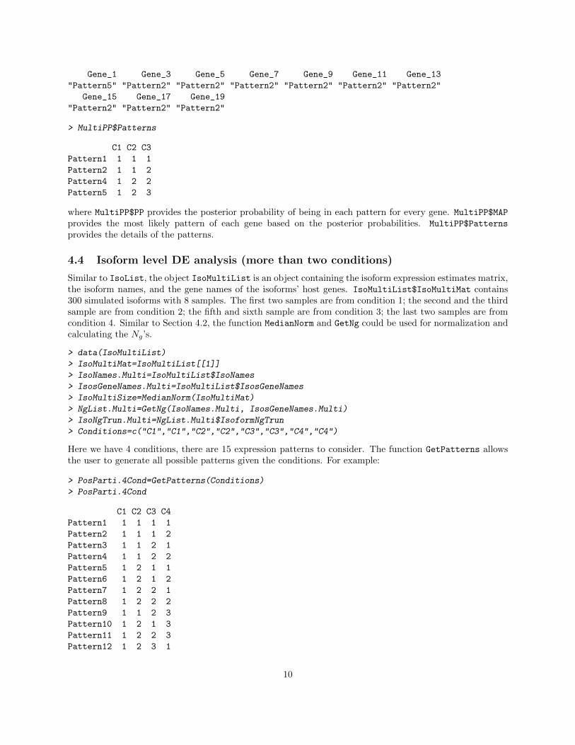
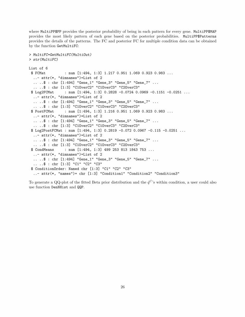
where MultiPP$PP provides the posterior probability of being in each pattern for every gene. MultiPP$MAP
provides the most likely pattern of each gene based on the posterior probabilities. MultiPP$Patterns
provides the details of the patterns.
4.4 Isoform level DE analysis (more than two conditions)
Similar to IsoList, the object IsoMultiList is an object containing the isoform expression estimates matrix,the isoform names, and the gene names of the isoforms’ host genes. IsoMultiList$IsoMultiMat contains300 simulated isoforms with 8 samples. The first two samples are from condition 1; the second and the thirdsample are from condition 2; the fifth and sixth sample are from condition 3; the last two samples are fromcondition 4. Similar to Section 4.2, the function MedianNorm and GetNg could be used for normalization andcalculating the Ng’s.
> data(IsoMultiList)
> IsoMultiMat=IsoMultiList[[1]]
> IsoNames.Multi=IsoMultiList$IsoNames
> IsosGeneNames.Multi=IsoMultiList$IsosGeneNames
> IsoMultiSize=MedianNorm(IsoMultiMat)
> NgList.Multi=GetNg(IsoNames.Multi, IsosGeneNames.Multi)
> IsoNgTrun.Multi=NgList.Multi$IsoformNgTrun
> Conditions=c("C1","C1","C2","C2","C3","C3","C4","C4")
Here we have 4 conditions, there are 15 expression patterns to consider. The function GetPatterns allowsthe user to generate all possible patterns given the conditions. For example:
> PosParti.4Cond=GetPatterns(Conditions)
> PosParti.4Cond
C1 C2 C3 C4
Pattern1 1 1 1 1
Pattern2 1 1 1 2
Pattern3 1 1 2 1
Pattern4 1 1 2 2
Pattern5 1 2 1 1
Pattern6 1 2 1 2
Pattern7 1 2 2 1
Pattern8 1 2 2 2
Pattern9 1 1 2 3
Pattern10 1 2 1 3
Pattern11 1 2 2 3
Pattern12 1 2 3 1
10

Pattern13 1 2 3 2
Pattern14 1 2 3 3
Pattern15 1 2 3 4
If we were interested in Patterns 1, 2, 3, 8 and 15 only, we’d define:
> Parti.4Cond=PosParti.4Cond[c(1,2,3,8,15),]
> Parti.4Cond
C1 C2 C3 C4
Pattern1 1 1 1 1
Pattern2 1 1 1 2
Pattern3 1 1 2 1
Pattern8 1 2 2 2
Pattern15 1 2 3 4
Moving on to the analysis, EBMultiTest could be used to perform the test:
> IsoMultiOut=EBMultiTest(IsoMultiMat,
+ NgVector=IsoNgTrun.Multi,Conditions=Conditions,
+ AllParti=Parti.4Cond, sizeFactors=IsoMultiSize,
+ maxround=5)
Removing transcripts with 75 th quantile < = 10
294 transcripts will be tested
The posterior probability of being in each pattern for every gene is obtained by using the function GetMultiPP:
> IsoMultiPP=GetMultiPP(IsoMultiOut)
> names(MultiPP)
[1] "PP" "MAP" "Patterns"
> IsoMultiPP$PP[1:10,]
Pattern1 Pattern2 Pattern3 Pattern8 Pattern15
Iso_1_1 3.533233e-32 0.999882138 3.408808e-33 2.143838e-34 1.178620e-04
Iso_1_2 4.231331e-14 0.999826487 1.573392e-16 5.848567e-18 1.735129e-04
Iso_1_3 5.633772e-47 0.992627423 5.963569e-42 5.644910e-50 7.372577e-03
Iso_1_4 4.248398e-35 0.998959777 1.983567e-30 5.054181e-33 1.040223e-03
Iso_1_5 0.000000e+00 1.000000000 0.000000e+00 0.000000e+00 1.584343e-41
Iso_1_6 1.509151e-232 0.002646919 3.147566e-220 6.720686e-188 9.973531e-01
Iso_1_7 2.835263e-138 0.999439469 7.548859e-133 1.613556e-128 5.605313e-04
Iso_1_8 9.654898e-139 0.963893542 3.709303e-105 5.626105e-120 3.610646e-02
Iso_1_9 1.947187e-47 0.957423511 1.073683e-50 3.868129e-46 4.257649e-02
Iso_1_10 7.904509e-08 0.999790300 9.178739e-10 9.386672e-10 2.096196e-04
> IsoMultiPP$MAP[1:10]
Iso_1_1 Iso_1_2 Iso_1_3 Iso_1_4 Iso_1_5 Iso_1_6
"Pattern2" "Pattern2" "Pattern2" "Pattern2" "Pattern2" "Pattern15"
Iso_1_7 Iso_1_8 Iso_1_9 Iso_1_10
"Pattern2" "Pattern2" "Pattern2" "Pattern2"
> IsoMultiPP$Patterns
11
C1 C2 C3 C4
Pattern1 1 1 1 1
Pattern2 1 1 1 2
Pattern3 1 1 2 1
Pattern8 1 2 2 2
Pattern15 1 2 3 4
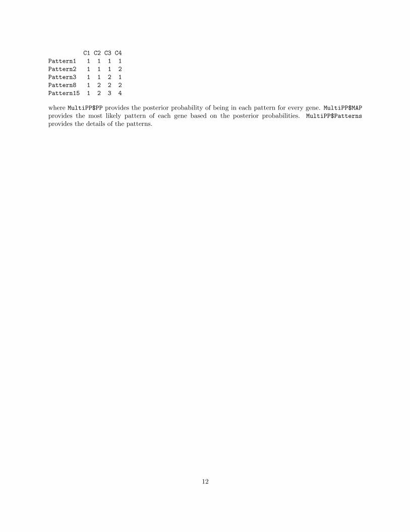
where MultiPP$PP provides the posterior probability of being in each pattern for every gene. MultiPP$MAP
provides the most likely pattern of each gene based on the posterior probabilities. MultiPP$Patterns
provides the details of the patterns.
12
5 More detailed examples
5.1 Gene level DE analysis (two conditions)
5.1.1 Running EBSeq on simulated gene expression estimates
EBSeq is applied as described in Section 4.1.3.
> data(GeneMat)
> Sizes=MedianNorm(GeneMat)
> EBOut=EBTest(Data=GeneMat,
+ Conditions=as.factor(rep(c("C1","C2"),each=5)),sizeFactors=Sizes, maxround=5)
> PP=GetPPMat(EBOut)
> str(PP)
num [1:950, 1:2] 0 0 0 0 0 ...
- attr(*, "dimnames")=List of 2
..$ : chr [1:950] "Gene_1" "Gene_2" "Gene_3" "Gene_4" ...
..$ : chr [1:2] "PPEE" "PPDE"
> head(PP)
PPEE PPDE
Gene_1 0.000000e+00 1
Gene_2 0.000000e+00 1
Gene_3 0.000000e+00 1
Gene_4 0.000000e+00 1
Gene_5 0.000000e+00 1
Gene_6 4.645857e-10 1
> DEfound=rownames(PP)[which(PP[,"PPDE"]>=.95)]
> str(DEfound)
chr [1:97] "Gene_1" "Gene_2" "Gene_3" "Gene_4" "Gene_5" ...
EBSeq found 98 DE genes at a target FDR of 0.05.
5.1.2 Calculating FC
The function PostFC may be used to calculate the Fold Change (FC) of the raw data as well as the posteriorFC of the normalized data. Figure 2 shows the FC vs. Posterior FC on 1,000 gene expression estimates.The genes are ranked by their cross-condition mean (adjusted by the normalization factors). The posteriorFC tends to shrink genes with low expressions (small rank); in this case the differences are minor.
13
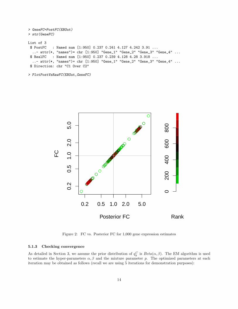
> GeneFC=PostFC(EBOut)
> str(GeneFC)
List of 3
$ PostFC : Named num [1:950] 0.237 0.241 4.127 4.242 3.91 ...
..- attr(*, "names")= chr [1:950] "Gene_1" "Gene_2" "Gene_3" "Gene_4" ...
$ RealFC : Named num [1:950] 0.237 0.239 4.128 4.28 3.918 ...
..- attr(*, "names")= chr [1:950] "Gene_1" "Gene_2" "Gene_3" "Gene_4" ...
$ Direction: chr "C1 Over C2"
> PlotPostVsRawFC(EBOut,GeneFC)
●●
●●●●
●●
●
●●
●
●●
●
●
●
●
●
●●●
●●●
●
●
●●
●
●
●
●
●
●
●
●●●
●●●
●
●
●
●
●●
●●
●●
●
●●
●
●
●
●
●●
●
●●
●
●●●
●
●
●
●
●
●●
●●
●
●
●
●
●
●●●
●●●
●
●●●
●●
●
●●●●●
●
●●
●
●●
●
●●●●●
●●●
●●●●●●●●●●●●
●●
●●
●●●
●●●●●
●●●●●
●●●
●●●●●●●
●●●●●
●●
●●●●
●●●●●●
●●●●●●
●
●●●●●●
●
●●●●●
●●
●
●●
●
●●●
●
●●
●
●
●●●●●
●●
●
●
●
●●●
●●●
●●●
●
●
●
●
●●●
●●●●●●●●●●
●
●
●●●●●●●
●●
●●●●●
●●●●
●●●●●
●●
●●●●●●●●●●●●●●
●
●●
●●●●
●
●●●
●●●●●●●●●●●
●●
●●
●●
●●●●
●
●●●●●
●●●●●●●
●
●●●
●●●●●
●●●●●●●●●
●
●
●●●●●●
●
●●
●●●●
●●●
●
●●
●
●●
●
●●●●●
●●
●●●●●
●●●●●
●●●
●●●
●●●●●●●●●●●
●●●
●●●●●●●●
●●●●●●
●●●●
●●●
●
●●
●
●●●●●
●●●●
●●●●●●●●
●●●●●●
●
●●●●●
●●●
●●●●
●●●●●●●●
●
●●
●●●●●
●●●
●●●●●
●●
●●●●
●●
●
●●●
●●
●●●
●
●●●●●●●●●●●●●●
●●●●●
●●
●●
●●●●●●●●●●
●●●●
●●●●●●
●
●●●
●●●
●
●
●●●●●●●●●
●●
●
●●●
●
●●
●●●●●●
●●
●●●●●
●
●
●
●
●●●●
●●●
●
●●●
●
●●●
●●
●●●●
●●●●●●●●●●●●●
●●
●●●●
●●●●
●●
●●●●●●●●
●●●●
●●●●
●●
●●
●●
●●
●●
●●●
●●●●
●
●●●●
●●●●●●
●●●●●●●●●●
●
●●●
●
●●●●●●●●
●
●●●●●●●●
●●
●●
●●●●●●
●●●●●
●●●●●
●●●●●●●●●●
●
●●●
●●
●●●●
●●●●
●
●●●●●●●●●
●
●●●●●
●●●
●●●
●●●●●
●
●●●●●●●
●●
●
●
●
●●
●●●●
●●●●
●●●
●●
●●
●●●●
●●●●●
●
●●●●●●●●
●●●
●
●●●●●●●●
●●●●
●
●●●●●
●
●●●●●●
●
●●●
●●●●●●●●●
●●
●
●●●●
●●●●
●●●●●●
●
●●●●
●
●●●●
●
●
●●●●●●●
●●●●●
●●●●●
●
●
●●
●
●●
●●●●●●●
●●●
●●●●●●
●●
0.2 0.5 1.0 2.0 5.0
0.2
0.5
1.0
2.0
5.0
Posterior FC
FC
020
040
060
080
0
Rank
Figure 2: FC vs. Posterior FC for 1,000 gene expression estimates
5.1.3 Checking convergence
As detailed in Section 3, we assume the prior distribution of qCg is Beta(α, β). The EM algorithm is usedto estimate the hyper-parameters α, β and the mixture parameter p. The optimized parameters at eachiteration may be obtained as follows (recall we are using 5 iterations for demonstration purposes):
14
> EBOut$Alpha
[,1]
iter1 0.8313646
iter2 0.8277784
iter3 0.8273499
iter4 0.8264807
iter5 0.8264807
> EBOut$Beta
Ng1
iter1 1.718970
iter2 1.721066
iter3 1.719731
iter4 1.716137
iter5 1.716137
> EBOut$P
[,1]
iter1 0.1693038
iter2 0.1338740
iter3 0.1289061
iter4 0.1284153
iter5 0.1284153
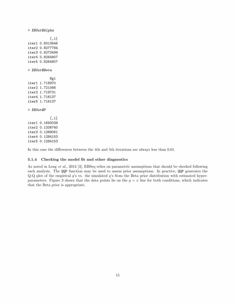
In this case the differences between the 4th and 5th iterations are always less than 0.01.
5.1.4 Checking the model fit and other diagnostics
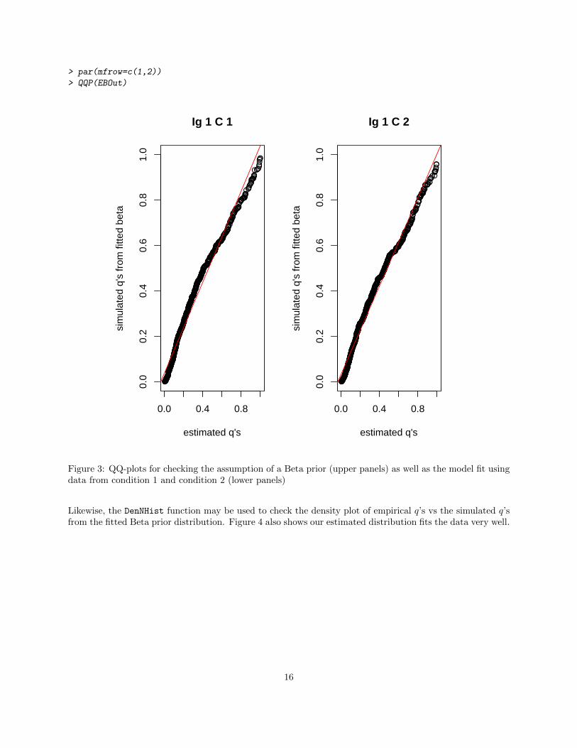
As noted in Leng et al., 2013 [3], EBSeq relies on parametric assumptions that should be checked followingeach analysis. The QQP function may be used to assess prior assumptions. In practice, QQP generates theQ-Q plot of the empirical q’s vs. the simulated q’s from the Beta prior distribution with estimated hyper-parameters. Figure 3 shows that the data points lie on the y = x line for both conditions, which indicatesthat the Beta prior is appropriate.
15
> par(mfrow=c(1,2))
> QQP(EBOut)
●●●●●●●●●●●●●●●●●●●●●●●●●●●●●●●●●●●●●●●●●●●●●●●●●●●●●●●●●●●●●●●●●●●●●●●●●●●●●●●●●●●●●●●●●●●●●●●●●●●●●●●●●●●●●●●●●●●●●●●●●●●●●●●●●●●●●●●●●●●●●●●●●●●●●●●●●●●●●●●●●●●●●●●●●●●●●●●●●●●●●●●●●●●●●●●●●●●●●●●●●●●●●●●●●●●●●●●●●●●●●●●●●●●●●●●●●●●●●●●●●●●●●●●●●●●●●●●●●●●●●●●●●●●●●●●●●●●●●●●●●●●●●●●●●●●●●●●●●●●●●●●●●●●●●●●●●●●●●●●●●●●●●●●●●●●●●●●●●●●●●●●●●●●●●●●●●●●●●●●●●●●●●●●●●●●●●●●●●●●●●●●●●●●●●●●●●●●●●●●●●●●●●●●●●●●●●●●●●●●●●●●●●●●●●●●●●●●●●●●●●●●●●●●●●●●●●●●●●●●●●●●●●●●●●●●●●●●●●●●●●●●●●●●●●●●●●●●●●●●●●●●●●●●●●●●●●●●●●●●●●●●●●●●●●●●●●●●●●●●●●●●●●●●●●●●●●●●●●●●●●●●●●●●●●●●●●●●●●●●●●●●●●●●●●●●●●●●●●●●●●●●●●●●●●●●●●●●●●●●●●●●●●●●●●●●●●●●●●●●●●●●●●●●●●●●●●●●●●●●●●●●●●●●●●●●●●●●●●●●●●●●●●●●●●●●●●●●●●●●●●●●●●●●●●●●●●●●●●●●●●●●●●●●●●●●●●●●●●●●●●●
●●●●●●●●●●●●●●●●●●●●●●●●●●●●●●●●●●●●●●●●●●●●●●●
●●●●●●
0.0 0.4 0.8
0.0
0.2
0.4
0.6
0.8
1.0
Ig 1 C 1
estimated q's
sim
ulat
ed q
's fr
om fi
tted
beta
●●●●●●●●●●●●●●●●●●●●●●●●●●●●●●●●●●●●●●●●●●●●●●●●●●●●●●●●●●●●●●●●●●●●●●●●●●●●●●●●●●●●●●●●●●●●●●●●●●●●●●●●●●●●●●●●●●●●●●●●●●●●●●●●●●●●●●●●●●●●●●●●●●●●●●●●●●●●●●●●●●●●●●●●●●●●●●●●●●●●●●●●●●●●●●●●●●●●●●●●●●●●●●●●●●●●●●●●●●●●●●●●●●●●●●●●●●●●●●●●●●●●●●●●●●●●●●●●●●●●●●●●●●●●●●●●●●●●●●●●●●●●●●●●●●●●●●●●●●●●●●●●●●●●●●●●●●●●●●●●●●●●●●●●●●●●●●●●●●●●●●●●●●●●●●●●●●●●●●●●●●●●●●●●●●●●●●●●●●●●●●●●●●●●●●●●●●●●●●●●●●●●●●●●●●●●●●●●●●●●●●●●●●●●●●●●●●●●●●●●●●●●●●●●●●●●●●●●●●●●●●●●●●●●●●●●●●●●●●●●●●●●●●●●●●●●●●●●●●●●●●●●●●●●●●●●●●●●●●●●●●●●●●●●●●●●●●●●●●●●●●●●●●●●●●●●●●●●●●●●●●●●●●●●●●●●●●●●●●●●●●●●●●●●●●●●●●●●●●●●●●●●●●●●●●●●●●●●●●●●●●●●●●●●●●●●●●●●●●●●●●●●●●●●●●●●●●●●●●●●●●●
●●●●●●●●●●●●●●●●●●●●●●●●●●●●●●●●●●●●●●●●●●●●●●●●●●●●●●●●●●●●●●●●●●●●●●●●●●●●●●●●●●●●●●●●●●●●●●●●●●●●●●●●●●●●●●●●●●●●●●
●●●●●●●●●
0.0 0.4 0.8
0.0
0.2
0.4
0.6
0.8
1.0
Ig 1 C 2
estimated q's
sim
ulat
ed q
's fr
om fi
tted
beta
Figure 3: QQ-plots for checking the assumption of a Beta prior (upper panels) as well as the model fit usingdata from condition 1 and condition 2 (lower panels)
Likewise, the DenNHist function may be used to check the density plot of empirical q’s vs the simulated q’sfrom the fitted Beta prior distribution. Figure 4 also shows our estimated distribution fits the data very well.
16

> par(mfrow=c(1,2))
> DenNHist(EBOut)
Ig 1 C 1
Q alpha=0.83 beta=1.72
Den
sity
0.0 0.4 0.8
01
23
4
DataFitted density
Ig 1 C 2
Q alpha=0.83 beta=1.72
Den
sity
0.0 0.4 0.8
01
23
4
DataFitted density
Figure 4: Density plots for checking the model fit using data from condition 1 and condition 2
5.2 Isoform level DE analysis (two conditions)
5.2.1 The Ig vector
Since EBSeq fits rely on Ig, we need to obtain the Ig for each isoform. This can be done using the functionGetNg. The required inputs of GetNg are the isoform names (IsoformNames) and their corresponding genenames (IsosGeneNames), described above. In the simulated data, we assume that the isoforms in theIg = 1 group belong to genes Gene_1, ... , Gene_200; The isoforms in the Ig = 2 group belong togenes Gene_201, ..., Gene_400; and isoforms in the Ig = 3 group belong to Gene_401, ..., Gene_600.
> data(IsoList)
> IsoMat=IsoList$IsoMat
> IsoNames=IsoList$IsoNames
> IsosGeneNames=IsoList$IsosGeneNames
> NgList=GetNg(IsoNames, IsosGeneNames, TrunThre=3)
17

> names(NgList)
[1] "GeneNg" "GeneNgTrun" "IsoformNg" "IsoformNgTrun"
> IsoNgTrun=NgList$IsoformNgTrun
> IsoNgTrun[c(1:3,201:203,601:603)]
Iso_1_1 Iso_1_2 Iso_1_3 Iso_2_1 Iso_2_2 Iso_2_3 Iso_3_1 Iso_3_2 Iso_3_3
1 1 1 2 2 2 3 3 3
The output of GetNg contains 4 vectors. GeneNg (IsoformNg) provides the number of isoforms Ng
within each gene (within each isoform’s host gene). GeneNgTrun (IsoformNgTrun) provides the Ig groupassignments. The default number of groups is 3, which means the isoforms with Ng greater than 3 will beassigned to Ig = 3 group. We use 3 in the case studies since the number of isoforms with Ng larger than 3is relatively small and the small sample size may induce poor parameter fitting if we treat them as separategroups. In practice, if there is evidence that the Ng = 4, 5, 6... groups should be treated as separate groups,a user can change TrunThre to define a different truncation threshold.
5.2.2 Using mappability ambiguity clusters instead of the Ig vector when the gene-isoformrelationship is unknown
When working with a de-novo assembled transcriptome, in which case the gene-isoform relationship is un-known, a user can use read mapping ambiguity cluster information instead of Ng, as provided by RSEM [4]in the output file output_name.ngvec. The file contains a vector with the same length as the total numberof transcripts. Each transcript has been assigned to one of 3 levels (1, 2, or 3) to indicate the mapping un-certainty level of that transcript. The mapping ambiguity clusters are partitioned via a k-means algorithmon the unmapability scores that are provided by RSEM. A user can read in the mapping ambiguity clusterinformation using:
> IsoNgTrun = scan(file="output_name.ngvec", what=0, sep="\n")
Where "output_name.ngvec" is the output file obtained from RSEM function rsem-generate-ngvector. Moredetails on using the RSEM-EBSeq pipeline on de novo assembled transcriptomes can be found at http:
//deweylab.biostat.wisc.edu/rsem/README.html#de.Other unmappability scores and other cluster methods (e.g. Gaussian Mixed Model) could also be used
to form the uncertainty clusters.
5.2.3 Running EBSeq on simulated isoform expression estimates
EBSeq can be applied as described in Section 4.2.4.
> IsoSizes=MedianNorm(IsoMat)
> IsoEBOut=EBTest(Data=IsoMat, NgVector=IsoNgTrun,
+ Conditions=as.factor(rep(c("C1","C2"),each=5)),sizeFactors=IsoSizes, maxround=5)
> IsoPP=GetPPMat(IsoEBOut)
> IsoDE=rownames(IsoPP)[which(IsoPP[,"PPDE"]>=.95)]
> str(IsoDE)
chr [1:106] "Iso_1_1" "Iso_1_2" "Iso_1_3" "Iso_1_4" "Iso_1_5" ...
We see that EBSeq found 105 DE isoforms at a target FDR of 0.05. The function PostFC could also be usedhere to calculate the Fold Change (FC) as well as the posterior FC on the normalization factor adjusteddata.
18

> IsoFC=PostFC(IsoEBOut)
> str(IsoFC)
List of 3
$ PostFC : Named num [1:1102] 0.286 0.281 3.553 0.305 3.755 ...
..- attr(*, "names")= chr [1:1102] "Iso_1_1" "Iso_1_2" "Iso_1_3" "Iso_1_4" ...
$ RealFC : Named num [1:1102] 0.285 0.281 3.556 0.305 3.759 ...
..- attr(*, "names")= chr [1:1102] "Iso_1_1" "Iso_1_2" "Iso_1_3" "Iso_1_4" ...
$ Direction: chr "C1 Over C2"
5.2.4 Checking convergence
For isoform level data, we assume the prior distribution of qCgi is Beta(α, βIg ). As in Section 5.1.3, theoptimized parameters at each iteration may be obtained as follows (recall we are using 5 iterations fordemonstration purposes):
> IsoEBOut$Alpha
[,1]
iter1 0.7321709
iter2 0.7881646
iter3 0.7885616
iter4 0.7877492
iter5 0.7867663
> IsoEBOut$Beta
Ng1 Ng2 Ng3
iter1 1.667405 2.648591 3.428080
iter2 1.833535 3.081309 4.453516
iter3 1.835056 3.092374 4.464689
iter4 1.838418 3.087711 4.464684
iter5 1.834517 3.082063 4.457264
> IsoEBOut$P
[,1]
iter1 0.2183707
iter2 0.1715496
iter3 0.1601954
iter4 0.1573053
iter5 0.1559198
Here we have 3 β’s in each iteration corresponding to βIg=1, βIg=2, βIg=3. We see that parameters arechanging less than 10−2 or 10−3. In practice, we require changes less than 10−3 to declare convergence.
5.2.5 Checking the model fit and other diagnostics
In Leng et al., 2013[3], we showed the mean-variance differences across different isoform groups on multipledata sets. In practice, if it is of interest to check differences among isoform groups defined by truncated Ig(such as those shown here in Figure 1), the function PolyFitPlot may be used. The following code generatesthe three panels shown in Figure 5 (if condition 2 is of interest, a user could change each C1 to C2.):
19

> par(mfrow=c(2,2))
> PolyFitValue=vector("list",3)
> for(i in 1:3)
+ PolyFitValue[[i]]=PolyFitPlot(IsoEBOut$C1Mean[[i]],
+ IsoEBOut$C1EstVar[[i]],5)
Estimated Mean
Est
imat
ed V
ar
0.1 1 10 1000 1e+05
0.1
101e
+05
Estimated MeanE
stim
ated
Var
0.1 1 10 1000 1e+05
0.1
101e
+05
Estimated Mean
Est
imat
ed V
ar
0.1 1 10 1000 1e+05
0.1
101e
+05
Figure 5: The mean-variance fitting plot for each Ng group
Superimposing all Ig groups using the code below will generate the figure (shown here in Figure 6), whichis similar in structure to Figure 1:
20
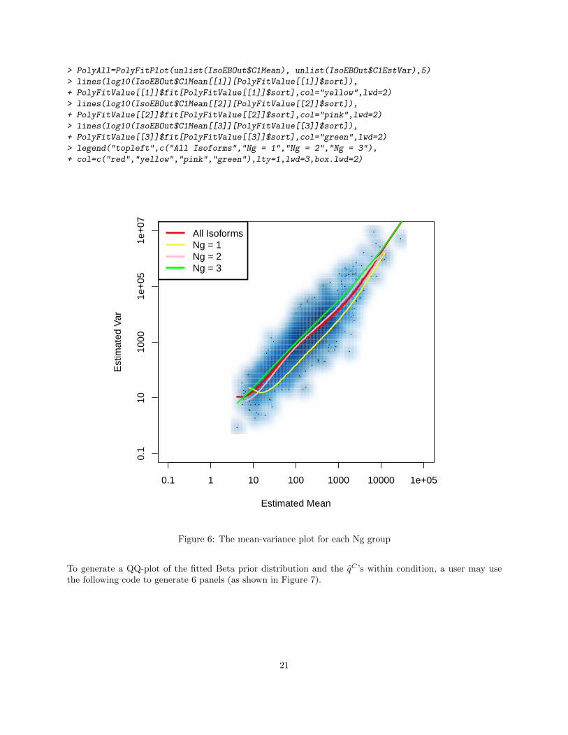
> PolyAll=PolyFitPlot(unlist(IsoEBOut$C1Mean), unlist(IsoEBOut$C1EstVar),5)
> lines(log10(IsoEBOut$C1Mean[[1]][PolyFitValue[[1]]$sort]),
+ PolyFitValue[[1]]$fit[PolyFitValue[[1]]$sort],col="yellow",lwd=2)
> lines(log10(IsoEBOut$C1Mean[[2]][PolyFitValue[[2]]$sort]),
+ PolyFitValue[[2]]$fit[PolyFitValue[[2]]$sort],col="pink",lwd=2)
> lines(log10(IsoEBOut$C1Mean[[3]][PolyFitValue[[3]]$sort]),
+ PolyFitValue[[3]]$fit[PolyFitValue[[3]]$sort],col="green",lwd=2)
> legend("topleft",c("All Isoforms","Ng = 1","Ng = 2","Ng = 3"),
+ col=c("red","yellow","pink","green"),lty=1,lwd=3,box.lwd=2)
Estimated Mean
Est
imat
ed V
ar
0.1 1 10 100 1000 10000 1e+05
0.1
1010
001e
+05
1e+
07
All IsoformsNg = 1Ng = 2Ng = 3
Figure 6: The mean-variance plot for each Ng group
To generate a QQ-plot of the fitted Beta prior distribution and the q̂C ’s within condition, a user may usethe following code to generate 6 panels (as shown in Figure 7).
21
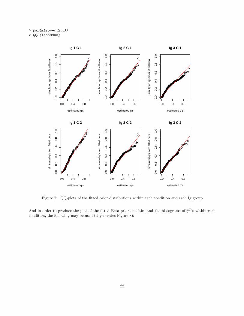
> par(mfrow=c(2,3))
> QQP(IsoEBOut)
●●●●●●●●●●●●●●●●●●●●●●●●●●●●●●●●●●●●●●●●●●●●●●●●●●●●●●●●●●●●●●●●●●●●●●●●●●●●●●●●●●●●●
●●●●●●●●●●●●●●●●●●●●●●●●●●●●●●●●●●●●●●●●●●●●●●●●
●●●●●●●●●●
●●●●●●
●●●●●●●
●●●●●●●●
●
●
0.0 0.4 0.8
0.0
0.2
0.4
0.6
0.8
1.0
Ig 1 C 1
estimated q's
sim
ulat
ed q
's fr
om fi
tted
beta
●●●●●●●●●●●●●●●●●●●●●●●●●●●●●●●●●●●●●●●●●●●●●●●●●●●●●●●●●●●●●●●●●●●●●●●●●●●●●●●●●●●●●●●●●●●●●●●●●●●●●●●●●●●●●●●●●●●●●●●●●●●●●●●●●●●●●●●●●●●●●●●●●●●●●●●●●●●●●●●●●●●●●●●●●●●●●●●●●●●●●●●●●●●●●●●●●●●●●●●●●●●●●●●●●●●●●●●●●●●●●●●●●●●●●●●●●●●●●●●●●●●●●●●●●●●●●●●●●●●●●●●●●●●●●●●●●●●●●●●●●
●●●●●●●●●●●●●●●●●●●●●●
●●●●●●●●●●●
●●●●●●●●●●
●●●●●●●●●
●●●●●●
●
●
●
0.0 0.4 0.80.
00.
20.
40.
60.
81.
0
Ig 2 C 1
estimated q's
sim
ulat
ed q
's fr
om fi
tted
beta
●●●●●●●●●●●●●●●●●●●●●●●●●●●●●●●●●●●●●●●●●●●●●●●●●●●●●●●●●●●●●●●●●●●●●●●●●●●●●●●●●●●●●●●●●●●●●●●●●●●●●●●●●●●●●●●●●●●●●●●●●●●●●●●●●●●●●●●●●●●●●●●●●●●●●●●●●●●●●●●●●●●●●●●●●●●●●●●●●●●●●●●●●●●●●●●●●●●●●●●●●●●●●●●●●●●●●●●●●●●●●●●●●●●●●●●●●●●●●●●●●●●●●●●●●●●●●●●●●●●●●●●●●●●●●●●●●●●●●●●●●●●●●●●●●●●●●●●●●●●●●●●●●●●●●●●●●●●●●●●●●●●●●●●●●●●●●●●●●●●●●●●●●●●●●●●●●●●●●●●●●●●●●●●●●●●●●●●●●●●●●●●●●●●●●●●●●●●●●●●●●●●●●●●●●●●●●●●●●●●●●●●●●●●●●●●●●●●●●●●●●●●●●●●●●●●●●●●●
●●●●●●●●●●●●●●●●●●●●
●●●●●●●●●●●●●●
●●●●●●●●
●●●●●●●●●
●●●●●●●●
●
0.0 0.4 0.8
0.0
0.2
0.4
0.6
0.8
1.0
Ig 3 C 1
estimated q's
sim
ulat
ed q
's fr
om fi
tted
beta
●●●●●●●●●●●●●●●●●●●●●●●●●●●●●●●●●●●●●●●●●●●●●●●●●●●●●●●●●●●●●●●●●●●●●●●●●●●●●●●●●●●●●●●●●●●●●●●●●●●●●●●●●●●●●●●●●●●●●●●●●●●●●●●●●●●●●●●●● ●●
●●●●●●●
●●●●●●●●
●●●●●
●●
●●●
●●
0.0 0.4 0.8
0.0
0.2
0.4
0.6
0.8
1.0
Ig 1 C 2
estimated q's
sim
ulat
ed q
's fr
om fi
tted
beta
●●●●●●●●●●●●●●●●●●●●●●●●●●●●●●●●●●●●●●●●●●●●●●●●●●●●●●●●●●●●●●●●●●●●●●●●●●●●●●●●●●●●●●●●●●●●●●●●●●●●●●●●●●●●●●●●●●●●●●●●●●●●●●●●●●●●●●●●●●●●●●●●●●●●●●●●●●●●●●●●●●●●●●●●●●●●●●●●●●●●●●●●●●●●●●●●●●●●●●●●●●●●●●●●●●●●●●●●●●●●●●●●●●●●●●●●●●●●●●●●●●●●●●
●●●●●●●●●●●●●●●●●●●●●●●●●●●●●●●●●●●●
●●●●●●●●●●●●●●●●●●●●●●
●●●●●●●●●●●●●●●●●
●●●●●●●●●●●●●●●●●●●●●●
●●●●●
●●
0.0 0.4 0.8
0.0
0.2
0.4
0.6
0.8
1.0
Ig 2 C 2
estimated q's
sim
ulat
ed q
's fr
om fi
tted
beta
●●●●●●●●●●●●●●●●●●●●●●●●●●●●●●●●●●●●●●●●●●●●●●●●●●●●●●●●●●●●●●●●●●●●●●●●●●●●●●●●●●●●●●●●●●●●●●●●●●●●●●●●●●●●●●●●●●●●●●●●●●●●●●●●●●●●●●●●●●●●●●●●●●●●●●●●●●●●●●●●●●●●●●●●●●●●●●●●●●●●●●●●●●●●●●●●●●●●●●●●●●●●●●●●●●●●●●●●●●●●●●●●●●●●●●●●●●●●●●●●●●●●●●●●●●●●●●●●●●●●●●●●●●●●●●●●●●●●●●●●●●●●●●●●●●●●●●●●●●●●●●●●●●●●●●●●●●●●●●●●●●●●●●●●●●●●●●●●●●●●●●●●●●●●●●●●●●●●●●●●●●●●●●●●●●●●●●●●●●●●●●●●●●●●●●●●●●●●●●●●●●●●●●●●●●●●●●●●●●●●●●●●●●●●●●●●●●●●●
●●●●●●●●●●●●●●●●●●●●●●●●●●●●●●●●●●●●
●●●●●●●●●●●●●
●●●●●●●●●●●●●●●●●●●●●
●●●●
●●●●●● ●
●
0.0 0.4 0.8
0.0
0.2
0.4
0.6
0.8
1.0
Ig 3 C 2
estimated q's
sim
ulat
ed q
's fr
om fi
tted
beta
Figure 7: QQ-plots of the fitted prior distributions within each condition and each Ig group
And in order to produce the plot of the fitted Beta prior densities and the histograms of q̂C ’s within eachcondition, the following may be used (it generates Figure 8):
22

> par(mfrow=c(2,3))
> DenNHist(IsoEBOut)
Ig 1 C 1
Q alpha=0.79 beta=1.83
Den
sity
0.0 0.4 0.8
01
23
DataFitted density
Ig 2 C 1
Q alpha=0.79 beta=3.08
Den
sity
0.0 0.4 0.8
01
23
45
6 DataFitted density
Ig 3 C 1
Q alpha=0.79 beta=4.46D
ensi
ty
0.0 0.4 0.8
02
46
DataFitted density
Ig 1 C 2
Q alpha=0.79 beta=1.83
Den
sity
0.0 0.4 0.8
01
23
45
6
DataFitted density
Ig 2 C 2
Q alpha=0.79 beta=3.08
Den
sity
0.0 0.4 0.8
02
46
8 DataFitted density
Ig 3 C 2
Q alpha=0.79 beta=4.46
Den
sity
0.0 0.4 0.8
02
46
8
DataFitted density
Figure 8: Prior distribution fit within each condition and each Ig group. (Note only a small set of isoformsare considered here for demonstration. Better fitting should be expected while using full set of isoforms.)
23
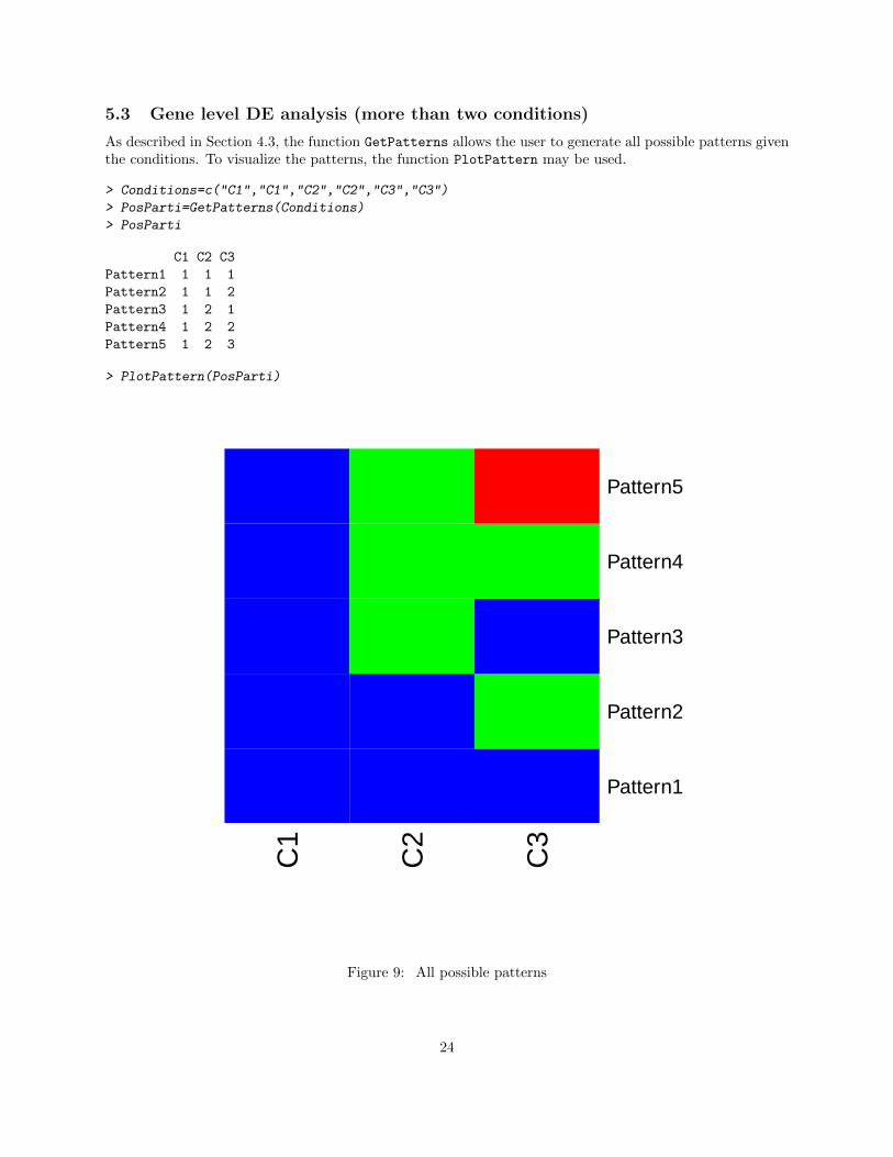
5.3 Gene level DE analysis (more than two conditions)
As described in Section 4.3, the function GetPatterns allows the user to generate all possible patterns giventhe conditions. To visualize the patterns, the function PlotPattern may be used.
> Conditions=c("C1","C1","C2","C2","C3","C3")
> PosParti=GetPatterns(Conditions)
> PosParti
C1 C2 C3
Pattern1 1 1 1
Pattern2 1 1 2
Pattern3 1 2 1
Pattern4 1 2 2
Pattern5 1 2 3
> PlotPattern(PosParti)
C1
C2
C3
Pattern1
Pattern2
Pattern3
Pattern4
Pattern5
Figure 9: All possible patterns
24

If we were interested in Patterns 1, 2, 4 and 5 only, we’d define:
> Parti=PosParti[-3,]
> Parti
C1 C2 C3
Pattern1 1 1 1
Pattern2 1 1 2
Pattern4 1 2 2
Pattern5 1 2 3
Moving on to the analysis, MedianNorm or one of its competitors should be used to determine the normal-ization factors. Once this is done, the formal test is performed by EBMultiTest.
> data(MultiGeneMat)
> MultiSize=MedianNorm(MultiGeneMat)
> MultiOut=EBMultiTest(MultiGeneMat,
+ NgVector=NULL,Conditions=Conditions,
+ AllParti=Parti, sizeFactors=MultiSize,
+ maxround=5)
The posterior probability of being in each pattern for every gene is obtained using the function GetMultiPP:
> MultiPP=GetMultiPP(MultiOut)
> names(MultiPP)
[1] "PP" "MAP" "Patterns"
> MultiPP$PP[1:10,]
Pattern1 Pattern2 Pattern4 Pattern5
Gene_1 8.533540e-94 0.3986838 5.107954e-72 0.60131622
Gene_3 9.691396e-164 0.9694403 6.680829e-109 0.03055971
Gene_5 6.243738e-26 0.9334990 6.351309e-20 0.06650097
Gene_7 0.000000e+00 0.5564474 0.000000e+00 0.44355263
Gene_9 5.019631e-16 0.9435967 2.013503e-15 0.05640325
Gene_11 1.945436e-11 0.9367403 2.163358e-12 0.06325967
Gene_13 1.426212e-08 0.7295369 6.405126e-10 0.27046313
Gene_15 3.485274e-47 0.9690530 8.526272e-41 0.03094699
Gene_17 3.336485e-184 0.6560285 4.551096e-133 0.34397147
Gene_19 1.744386e-37 0.9042735 1.311200e-24 0.09572651
> MultiPP$MAP[1:10]
Gene_1 Gene_3 Gene_5 Gene_7 Gene_9 Gene_11 Gene_13
"Pattern5" "Pattern2" "Pattern2" "Pattern2" "Pattern2" "Pattern2" "Pattern2"
Gene_15 Gene_17 Gene_19
"Pattern2" "Pattern2" "Pattern2"
> MultiPP$Patterns
C1 C2 C3
Pattern1 1 1 1
Pattern2 1 1 2
Pattern4 1 2 2
Pattern5 1 2 3
25
where MultiPP$PP provides the posterior probability of being in each pattern for every gene. MultiPP$MAP
provides the most likely pattern of each gene based on the posterior probabilities. MultiPP$Patterns
provides the details of the patterns. The FC and posterior FC for multiple condition data can be obtainedby the function GetMultiFC:
> MultiFC=GetMultiFC(MultiOut)
> str(MultiFC)
List of 6
$ FCMat : num [1:494, 1:3] 1.217 0.951 1.069 0.923 0.983 ...
..- attr(*, "dimnames")=List of 2
.. ..$ : chr [1:494] "Gene_1" "Gene_3" "Gene_5" "Gene_7" ...
.. ..$ : chr [1:3] "C1OverC2" "C1OverC3" "C2OverC3"
$ Log2FCMat : num [1:494, 1:3] 0.2828 -0.0724 0.0969 -0.1151 -0.0251 ...
..- attr(*, "dimnames")=List of 2
.. ..$ : chr [1:494] "Gene_1" "Gene_3" "Gene_5" "Gene_7" ...
.. ..$ : chr [1:3] "C1OverC2" "C1OverC3" "C2OverC3"
$ PostFCMat : num [1:494, 1:3] 1.216 0.951 1.069 0.923 0.983 ...
..- attr(*, "dimnames")=List of 2
.. ..$ : chr [1:494] "Gene_1" "Gene_3" "Gene_5" "Gene_7" ...
.. ..$ : chr [1:3] "C1OverC2" "C1OverC3" "C2OverC3"
$ Log2PostFCMat : num [1:494, 1:3] 0.2819 -0.072 0.0967 -0.115 -0.0251 ...
..- attr(*, "dimnames")=List of 2
.. ..$ : chr [1:494] "Gene_1" "Gene_3" "Gene_5" "Gene_7" ...
.. ..$ : chr [1:3] "C1OverC2" "C1OverC3" "C2OverC3"
$ CondMeans : num [1:494, 1:3] 499 253 813 1843 753 ...
..- attr(*, "dimnames")=List of 2
.. ..$ : chr [1:494] "Gene_1" "Gene_3" "Gene_5" "Gene_7" ...
.. ..$ : chr [1:3] "C1" "C2" "C3"
$ ConditionOrder: Named chr [1:3] "C1" "C2" "C3"
..- attr(*, "names")= chr [1:3] "Condition1" "Condition2" "Condition3"
To generate a QQ-plot of the fitted Beta prior distribution and the q̂C ’s within condition, a user could alsouse function DenNHist and QQP.
26

> par(mfrow=c(2,2))
> QQP(MultiOut)
●●●●●●●●●●●●●●●●●●●●●●●●●●●●●●●●●●●●●●●●●●●●●●●●●●●●
●●●●●●●●●●●●●●●●●●●●●●●●●●●●●●●●●●●●●●●●●●●●●●
●●●●●●●●●●●●●●●●●●●●●●●●●●●●●●●
●●●●●●●●●●●●●●●●●●●●●●●●●●●●
●●●●●●●●●●●●●●●●●●●●●●●●●●●
●●●●●●●●●●●●●●●●●●●
●●●●●●●●●●●●●●●●●●●
●●●●●●●●●●●●●●●●
●●●●●●●●●●●●●●●
●●●●●●●●●●●●●
●●●●●●●
0.0 0.2 0.4 0.6 0.8 1.0
0.0
0.4
0.8
Ig 1 C 1
estimated q's
sim
ulat
ed q
's fr
om fi
tted
beta
●●●●●●●●●●●●●●●●●●●●●●●●●●●●●●●●●●●●●●●●●●●●●●●●●●●●●●●●●●●●●●
●●●●●●●●●●●●●●●●●●●●●●●●●●●●●●●●●●●●●
●●●●●●●●●●●●●●●●●●●●●●●●●●●●●●●●●●●●●●●●●●●
●●●●●●●●●●●●●●●●●●●●●●●●●●●●●●●●●
●●●●●●●●●●●●●●●●●●●●●●●●●●●●●●
●●●●●●●●●●●●●●●●●●●●●
●●●●●●●●●●●●
●●●●●●●●
●●●●●●●●●●●●●●
●●●●●●●●●
●●●●●●
0.0 0.2 0.4 0.6 0.8 1.0
0.0
0.4
0.8
Ig 1 C 2
estimated q's
sim
ulat
ed q
's fr
om fi
tted
beta
●●●●●●●●●●●●●●●●●●●●●●●●●●●●●●●●●●●●●●●●●●●●●●●●●●●●●●●●●●●●●●●●●●●●●●●●●
●●●●●●●●●●●●●●●●●●●●●●●●●●●●●●●●●●●●●●●●●●●●●●●●●●●●
●●●●●●●●●●●●●●●●●●●●●●●●●●●●●●●●●●
●●●●●●●●●●●●●●●●●●●●●●●●●●●●●
●●●●●●●●●●●●●●●●●●●●●
●●●●●●●●●●●●●●●
●●●●●●●●●●●●●●●●●●●●●●●
●●●●●●●●●●●●●●●●
●●●●●●●●●●●
●●●●●●●●●●●●●●
●●●●●●
0.0 0.2 0.4 0.6 0.8 1.0
0.0
0.4
0.8
Ig 1 C 3
estimated q's
sim
ulat
ed q
's fr
om fi
tted
beta
Figure 10: QQ-plots of the fitted prior distributions within each condition and each Ig group
27
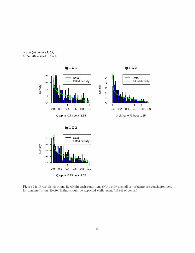
> par(mfrow=c(2,2))
> DenNHist(MultiOut)
Ig 1 C 1
Q alpha=0.73 beta=1.55
Den
sity
0.0 0.2 0.4 0.6 0.8 1.0
01
23
4
DataFitted density
Ig 1 C 2
Q alpha=0.73 beta=1.55
Den
sity
0.0 0.2 0.4 0.6 0.8 1.00
12
34
5 DataFitted density
Ig 1 C 3
Q alpha=0.73 beta=1.55
Den
sity
0.0 0.2 0.4 0.6 0.8 1.0
01
23
4 DataFitted density
Figure 11: Prior distributions fit within each condition. (Note only a small set of genes are considered herefor demonstration. Better fitting should be expected while using full set of genes.)
28
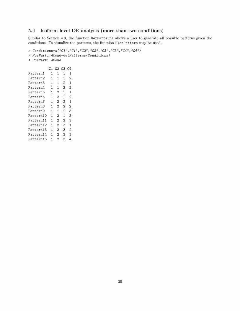
5.4 Isoform level DE analysis (more than two conditions)
Similar to Section 4.3, the function GetPatterns allows a user to generate all possible patterns given theconditions. To visualize the patterns, the function PlotPattern may be used.
> Conditions=c("C1","C1","C2","C2","C3","C3","C4","C4")
> PosParti.4Cond=GetPatterns(Conditions)
> PosParti.4Cond
C1 C2 C3 C4
Pattern1 1 1 1 1
Pattern2 1 1 1 2
Pattern3 1 1 2 1
Pattern4 1 1 2 2
Pattern5 1 2 1 1
Pattern6 1 2 1 2
Pattern7 1 2 2 1
Pattern8 1 2 2 2
Pattern9 1 1 2 3
Pattern10 1 2 1 3
Pattern11 1 2 2 3
Pattern12 1 2 3 1
Pattern13 1 2 3 2
Pattern14 1 2 3 3
Pattern15 1 2 3 4
29
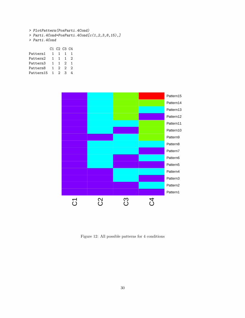
> PlotPattern(PosParti.4Cond)
> Parti.4Cond=PosParti.4Cond[c(1,2,3,8,15),]
> Parti.4Cond
C1 C2 C3 C4
Pattern1 1 1 1 1
Pattern2 1 1 1 2
Pattern3 1 1 2 1
Pattern8 1 2 2 2
Pattern15 1 2 3 4C
1
C2
C3
C4
Pattern1
Pattern2
Pattern3
Pattern4
Pattern5
Pattern6
Pattern7
Pattern8
Pattern9
Pattern10
Pattern11
Pattern12
Pattern13
Pattern14
Pattern15
Figure 12: All possible patterns for 4 conditions
30
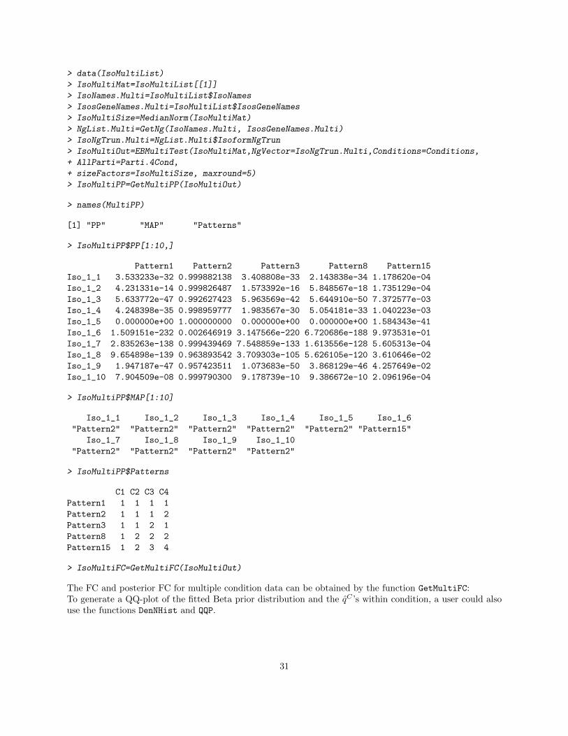
> data(IsoMultiList)
> IsoMultiMat=IsoMultiList[[1]]
> IsoNames.Multi=IsoMultiList$IsoNames
> IsosGeneNames.Multi=IsoMultiList$IsosGeneNames
> IsoMultiSize=MedianNorm(IsoMultiMat)
> NgList.Multi=GetNg(IsoNames.Multi, IsosGeneNames.Multi)
> IsoNgTrun.Multi=NgList.Multi$IsoformNgTrun
> IsoMultiOut=EBMultiTest(IsoMultiMat,NgVector=IsoNgTrun.Multi,Conditions=Conditions,
+ AllParti=Parti.4Cond,
+ sizeFactors=IsoMultiSize, maxround=5)
> IsoMultiPP=GetMultiPP(IsoMultiOut)
> names(MultiPP)
[1] "PP" "MAP" "Patterns"
> IsoMultiPP$PP[1:10,]
Pattern1 Pattern2 Pattern3 Pattern8 Pattern15
Iso_1_1 3.533233e-32 0.999882138 3.408808e-33 2.143838e-34 1.178620e-04
Iso_1_2 4.231331e-14 0.999826487 1.573392e-16 5.848567e-18 1.735129e-04
Iso_1_3 5.633772e-47 0.992627423 5.963569e-42 5.644910e-50 7.372577e-03
Iso_1_4 4.248398e-35 0.998959777 1.983567e-30 5.054181e-33 1.040223e-03
Iso_1_5 0.000000e+00 1.000000000 0.000000e+00 0.000000e+00 1.584343e-41
Iso_1_6 1.509151e-232 0.002646919 3.147566e-220 6.720686e-188 9.973531e-01
Iso_1_7 2.835263e-138 0.999439469 7.548859e-133 1.613556e-128 5.605313e-04
Iso_1_8 9.654898e-139 0.963893542 3.709303e-105 5.626105e-120 3.610646e-02
Iso_1_9 1.947187e-47 0.957423511 1.073683e-50 3.868129e-46 4.257649e-02
Iso_1_10 7.904509e-08 0.999790300 9.178739e-10 9.386672e-10 2.096196e-04
> IsoMultiPP$MAP[1:10]
Iso_1_1 Iso_1_2 Iso_1_3 Iso_1_4 Iso_1_5 Iso_1_6
"Pattern2" "Pattern2" "Pattern2" "Pattern2" "Pattern2" "Pattern15"
Iso_1_7 Iso_1_8 Iso_1_9 Iso_1_10
"Pattern2" "Pattern2" "Pattern2" "Pattern2"
> IsoMultiPP$Patterns
C1 C2 C3 C4
Pattern1 1 1 1 1
Pattern2 1 1 1 2
Pattern3 1 1 2 1
Pattern8 1 2 2 2
Pattern15 1 2 3 4
> IsoMultiFC=GetMultiFC(IsoMultiOut)
The FC and posterior FC for multiple condition data can be obtained by the function GetMultiFC:To generate a QQ-plot of the fitted Beta prior distribution and the q̂C ’s within condition, a user could alsouse the functions DenNHist and QQP.
31
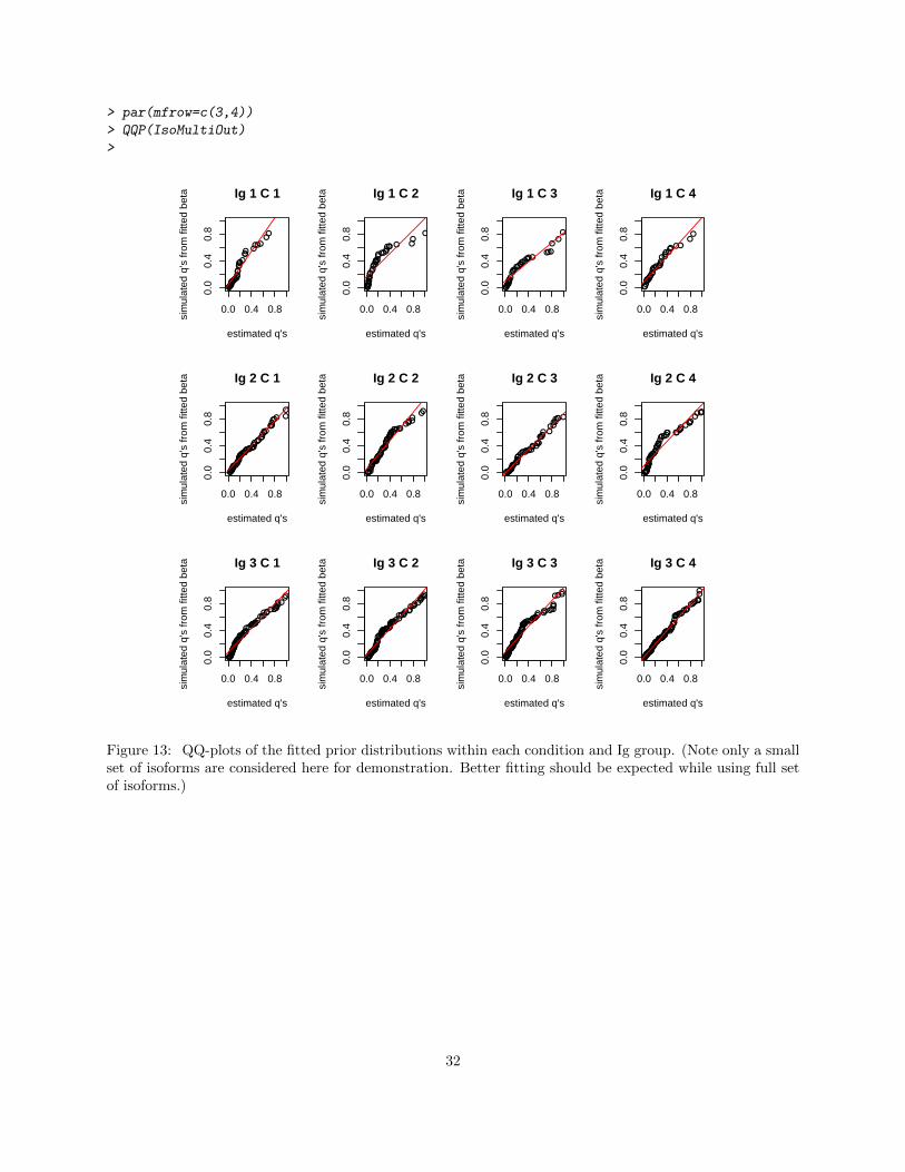
> par(mfrow=c(3,4))
> QQP(IsoMultiOut)
>
●●●●●●●●●●●●●●●
●●●●●●●●●●
●●●●●●●
●●
0.0 0.4 0.8
0.0
0.4
0.8
Ig 1 C 1
estimated q's
sim
ulat
ed q
's fr
om fi
tted
beta
●●●●●●●●●●●●●●●●●●●●●●●●●●●
●●●●●●● ● ●
●●
0.0 0.4 0.8
0.0
0.4
0.8
Ig 1 C 2
estimated q'ssi
mul
ated
q's
from
fitte
d be
ta
●●●●●●●●●●●●●●●●●
●●●●●●●●
●●●●●●●
●●
●
0.0 0.4 0.8
0.0
0.4
0.8
Ig 1 C 3
estimated q's
sim
ulat
ed q
's fr
om fi
tted
beta
●●●●●●●●●●●●●●●●●●
●●●●●●●●●
●●●●●●
●●
0.0 0.4 0.8
0.0
0.4
0.8
Ig 1 C 4
estimated q's
sim
ulat
ed q
's fr
om fi
tted
beta
●●●●●●●●●●●●●●●●
●●●●●●●●●●●●●●
●●●●●●●●●●●●●●
●●●●●●
●●●●●●● ●
●
0.0 0.4 0.8
0.0
0.4
0.8
Ig 2 C 1
estimated q's
sim
ulat
ed q
's fr
om fi
tted
beta
●●●●●●●●●●●●●●●●●
●●●●●●●●●●●●●●●●●●●●●●●●●●●●●●●●
●●●●●
●●
●●
0.0 0.4 0.8
0.0
0.4
0.8
Ig 2 C 2
estimated q's
sim
ulat
ed q
's fr
om fi
tted
beta
●●●●●●●●●●●●●●●●●●●
●●●●●●●
●●●●●●●●●●●●●
●●●●● ●
●●●●●●●●
0.0 0.4 0.80.
00.
40.
8
Ig 2 C 3
estimated q's
sim
ulat
ed q
's fr
om fi
tted
beta
●●●●●●●●●●●●●●●●●●●●●●●●●●●●●●●●●●●●●●●●
●● ●●●●●●●●●
●●●●
0.0 0.4 0.8
0.0
0.4
0.8
Ig 2 C 4
estimated q's
sim
ulat
ed q
's fr
om fi
tted
beta
●●●●●●●●●●●●●●●●●●●●●●●●●●●●●●●●●●●●●●●●●●●●●●●●●●●●●●●●●●●●●●●●
●●●●●●●
●●●●●●●●
●●
0.0 0.4 0.8
0.0
0.4
0.8
Ig 3 C 1
estimated q's
sim
ulat
ed q
's fr
om fi
tted
beta
●●●●●●●●●●●●●●●●●●●●
●●●●●●●●●●●●●●●●●●●●●●●●
●●●●●●●●●●●●●●
●●●●●●●●●●
●●●●●●●
●●●●●●●
●●●●●●●
0.0 0.4 0.8
0.0
0.4
0.8
Ig 3 C 2
estimated q's
sim
ulat
ed q
's fr
om fi
tted
beta
●●●●●●●●●●●●●●●●●●●●●●●●●●●●●●●●●●●●●●●●●●●●●●●●●●●●●●●●●●●●●●●●●
●●●● ●●●●●●
●●
●●●●
0.0 0.4 0.8
0.0
0.4
0.8
Ig 3 C 3
estimated q's
sim
ulat
ed q
's fr
om fi
tted
beta
●●●●●●●●●●●●●●●●●●●●●●●●
●●●●●●●●●●●●●●●●●●●●●●●●●●●●
●●●●●●●●●●●●●●
●●●●●●●●●●●●●
●●●●●
●●●●●●●●●
0.0 0.4 0.8
0.0
0.4
0.8
Ig 3 C 4
estimated q's
sim
ulat
ed q
's fr
om fi
tted
beta
Figure 13: QQ-plots of the fitted prior distributions within each condition and Ig group. (Note only a smallset of isoforms are considered here for demonstration. Better fitting should be expected while using full setof isoforms.)
32
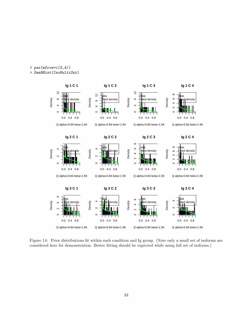
> par(mfrow=c(3,4))
> DenNHist(IsoMultiOut)
Ig 1 C 1
Q alpha=0.84 beta=1.94
Den
sity
0.0 0.4 0.8
04
812
DataFitted density
Ig 1 C 2
Q alpha=0.84 beta=1.94
Den
sity
0.0 0.4 0.8
04
812 Data
Fitted density
Ig 1 C 3
Q alpha=0.84 beta=1.94D
ensi
ty
0.0 0.4 0.8
04
812
DataFitted density
Ig 1 C 4
Q alpha=0.84 beta=1.94
Den
sity
0.0 0.4 0.8
02
46
8 DataFitted density
Ig 2 C 1
Q alpha=0.84 beta=1.59
Den
sity
0.0 0.4 0.8
02
4 DataFitted density
Ig 2 C 2
Q alpha=0.84 beta=1.59
Den
sity
0.0 0.4 0.8
02
4 DataFitted density
Ig 2 C 3
Q alpha=0.84 beta=1.59
Den
sity
0.0 0.4 0.8
02
46
8
DataFitted density
Ig 2 C 4
Q alpha=0.84 beta=1.59
Den
sity
0.0 0.4 0.8
02
46
8 DataFitted density
Ig 3 C 1
Q alpha=0.84 beta=1.56
Den
sity
0.0 0.4 0.8
02
46
DataFitted density
Ig 3 C 2
Q alpha=0.84 beta=1.56
Den
sity
0.0 0.4 0.8
02
4
DataFitted density
Ig 3 C 3
Q alpha=0.84 beta=1.56
Den
sity
0.0 0.4 0.8
02
46 Data
Fitted density
Ig 3 C 4
Q alpha=0.84 beta=1.56
Den
sity
0.0 0.4 0.8
02
4
DataFitted density
Figure 14: Prior distributions fit within each condition and Ig group. (Note only a small set of isoforms areconsidered here for demonstration. Better fitting should be expected while using full set of isoforms.)
33
5.5 Working without replicates
When replicates are not available, it is difficult to estimate the transcript specific variance. In this case,EBSeq estimates the variance by pooling similar genes together. Specifically, we take genes with FC in the25% - 75% quantile of all FC’s as candidate genes. By defining NumBin = 1000 (default in EBTest), EBSeqwill group genes with similar means into 1,000 bins. For each candidate gene, we use the across-conditionvariance estimate as its variance estimate. For each bin, the bin-wise variance estimation is taken to bethe median of the across-condition variance estimates of the candidate genes within that bin. For eachnon-candidate gene, we use the bin-wise variance estimate of the host bin (the bin containing this gene) asits variance estimate. This approach works well when there are no more than 50% DE genes in the data set.
5.5.1 Gene counts with two conditions
To generate a data set with no replicates, we take the first sample of each condition. For example, usingthe data from Section 5.1, we take sample 1 from condition 1 and sample 6 from condition 2. FunctionsMedianNorm, GetPPMat and PostFC may be used on data without replicates.
> data(GeneMat)
> GeneMat.norep=GeneMat[,c(1,6)]
> Sizes.norep=MedianNorm(GeneMat.norep)
> EBOut.norep=EBTest(Data=GeneMat.norep,
+ Conditions=as.factor(rep(c("C1","C2"))),
+ sizeFactors=Sizes.norep, maxround=5)
Removing transcripts with 75 th quantile < = 10
938 transcripts will be tested
> PP.norep=GetPPMat(EBOut.norep)
> DEfound.norep=rownames(PP.norep)[which(PP.norep[,"PPDE"]>=.95)]
> GeneFC.norep=PostFC(EBOut.norep)
5.5.2 Isoform counts with two conditions
To generate an isoform level data set with no replicates, we also take sample 1 and sample 6 in the data weused in Section 5.2. Example codes are shown below.
> data(IsoList)
> IsoMat=IsoList$IsoMat
> IsoNames=IsoList$IsoNames
> IsosGeneNames=IsoList$IsosGeneNames
> NgList=GetNg(IsoNames, IsosGeneNames)
> IsoNgTrun=NgList$IsoformNgTrun
> IsoMat.norep=IsoMat[,c(1,6)]
> IsoSizes.norep=MedianNorm(IsoMat.norep)
> IsoEBOut.norep=EBTest(Data=IsoMat.norep, NgVector=IsoNgTrun,
+ Conditions=as.factor(c("C1","C2")),
+ sizeFactors=IsoSizes.norep, maxround=5)
Removing transcripts with 75 th quantile < = 10
1088 transcripts will be tested
> IsoPP.norep=GetPPMat(IsoEBOut.norep)
> IsoDE.norep=rownames(IsoPP.norep)[which(IsoPP.norep[,"PPDE"]>=.95)]
> IsoFC.norep=PostFC(IsoEBOut.norep)
34
5.5.3 Gene counts with more than two conditions
To generate a data set with multiple conditions and no replicates, we take the first sample from each condition(sample 1, 3 and 5) in the data we used in Section 5.3. Example codes are shown below.
> data(MultiGeneMat)
> MultiGeneMat.norep=MultiGeneMat[,c(1,3,5)]
> Conditions=c("C1","C2","C3")
> PosParti=GetPatterns(Conditions)
> Parti=PosParti[-3,]
> MultiSize.norep=MedianNorm(MultiGeneMat.norep)
> MultiOut.norep=EBMultiTest(MultiGeneMat.norep,
+ NgVector=NULL,Conditions=Conditions,
+ AllParti=Parti, sizeFactors=MultiSize.norep,
+ maxround=5)
Removing transcripts with 75 th quantile < = 10
492 transcripts will be tested
> MultiPP.norep=GetMultiPP(MultiOut.norep)
> MultiFC.norep=GetMultiFC(MultiOut.norep)
5.5.4 Isoform counts with more than two conditions
To generate an isoform level data set with multiple conditions and no replicates, we take the first samplefrom each condition (sample 1, 3, 5 and 7) in the data we used in Section 5.4. Example codes are shownbelow.
> data(IsoMultiList)
> IsoMultiMat=IsoMultiList[[1]]
> IsoNames.Multi=IsoMultiList$IsoNames
> IsosGeneNames.Multi=IsoMultiList$IsosGeneNames
> IsoMultiMat.norep=IsoMultiMat[,c(1,3,5,7)]
> IsoMultiSize.norep=MedianNorm(IsoMultiMat.norep)
> NgList.Multi=GetNg(IsoNames.Multi, IsosGeneNames.Multi)
> IsoNgTrun.Multi=NgList.Multi$IsoformNgTrun
> Conditions=c("C1","C2","C3","C4")
> PosParti.4Cond=GetPatterns(Conditions)
> PosParti.4Cond
C1 C2 C3 C4
Pattern1 1 1 1 1
Pattern2 1 1 1 2
Pattern3 1 1 2 1
Pattern4 1 1 2 2
Pattern5 1 2 1 1
Pattern6 1 2 1 2
Pattern7 1 2 2 1
Pattern8 1 2 2 2
Pattern9 1 1 2 3
Pattern10 1 2 1 3
Pattern11 1 2 2 3
Pattern12 1 2 3 1
Pattern13 1 2 3 2
35
Pattern14 1 2 3 3
Pattern15 1 2 3 4
> Parti.4Cond=PosParti.4Cond[c(1,2,3,8,15),]
> Parti.4Cond
C1 C2 C3 C4
Pattern1 1 1 1 1
Pattern2 1 1 1 2
Pattern3 1 1 2 1
Pattern8 1 2 2 2
Pattern15 1 2 3 4
> IsoMultiOut.norep=EBMultiTest(IsoMultiMat.norep,
+ NgVector=IsoNgTrun.Multi,Conditions=Conditions,
+ AllParti=Parti.4Cond, sizeFactors=IsoMultiSize.norep,
+ maxround=5)
Removing transcripts with 75 th quantile < = 10
293 transcripts will be tested
> IsoMultiPP.norep=GetMultiPP(IsoMultiOut.norep)
> IsoMultiFC.norep=GetMultiFC(IsoMultiOut.norep)
6 EBSeq pipelines and extensions
6.1 RSEM-EBSeq pipeline: from raw reads to differential expression analysisresults
EBSeq is coupled with RSEM [4] as an RSEM-EBSeq pipeline which provides quantification and DE testingon both gene and isoform levels.
For more details, see http://deweylab.biostat.wisc.edu/rsem/README.html#de
6.2 EBSeq interface: A user-friendly graphical interface for differetial expres-sion analysis
EBSeq interface provides a graphical interface implementation for users who are not familiar with the Rprogramming language. It takes .xls, .xlsx and .csv files as input. Additional packages need be downloaded;they may be found at http://www.biostat.wisc.edu/~ningleng/EBSeq_Package/EBSeq_Interface/
6.3 EBSeq Galaxy tool shed
EBSeq tool shed contains EBSeq wrappers for a local Galaxy implementation. For more details, see http:
//www.biostat.wisc.edu/~ningleng/EBSeq_Package/EBSeq_Galaxy_toolshed/
7 Acknowledgment
We would like to thank Haolin Xu for checking the package and proofreading the vignette.
36

8 News
2014-1-30: In EBSeq 1.3.3, the default setting of EBTest function will remove low expressed genes (geneswhose 75th quantile of normalized counts is less than 10) before identifying DE genes. These two thresholdscan be changed in EBTest function. We found that low expressed genes are more easily to be affectedby noises. Removing these genes prior to downstream analyses can improve the model fitting and reduceimpacts of noisy genes (e.g. genes with outliers).
2014-5-22: In EBSeq 1.5.2, numerical approximations are implemented to deal with underflow. Theunderflow is likely due to large number of samples.
37

References
[1] S Anders and W Huber. Differential expression analysis for sequence count data. Genome Biology,11:R106, 2010.
[2] J H Bullard, E A Purdom, K D Hansen, and S Dudoit. Evaluation of statistical methods for normalizationand differential expression in mrna-seq experiments. BMC Bioinformatics, 11:94, 2010.
[3] Ning Leng, John A Dawson, James A Thomson, Victor Ruotti, Anna I Rissman, Bart MG Smits,Jill D Haag, Michael N Gould, Ron M Stewart, and Christina Kendziorski. Ebseq: an empirical bayeshierarchical model for inference in rna-seq experiments. Bioinformatics, 29(8):1035–1043, 2013.
[4] B Li and C N Dewey. Rsem: accurate transcript quantification from rna-seq data with or without areference genome. BMC Bioinformatics, 12:323, 2011.
[5] M D Robinson and A Oshlack. A scaling normalization method for differential expression analysis ofrna-seq data. Genome Biology, 11:R25, 2010.
[6] C Trapnell, A Roberts, L Goff, G Pertea, D Kim, D R Kelley, H Pimentel, S L Salzberg, J L Rinn, andL Pachter. Differential gene and transcript expression analysis of rna-seq experiments with tophat andcufflinks. Nature Protocols, 7(3):562–578, 2012.
38