EARTHQUAKE SITE RESPONSE ANALYSES FOR SOIL NASIM …studentsrepo.um.edu.my/9234/8/Nasim_Sarrafi_Aghdam-Thesis_201… · Tajuk Kertas Prokjek/Laporan Penyelidikan/ Disertasi/Tesis

EARTHQUAKE SITE RESPONSE ANALYSES FOR SOIL

CONDITIONS OF SEVERAL CITIES IN MALAYSIA

NASIM SARRAFI AGHDAM

DISSERTATION SUBMITTED IN FULFILMENT OF THE

REQUIREMENTS FOR THE DEGREE OF MASTER OF

ENGINEERING SCIENCE

FACULTY OF ENGINEERING

UNIVERSITY OF MALAYA

KUALA LUMPUR

2017

ii

UNIVERSITI MALAYA

ORIGINAL LITERARY WORK DECLARATION

Name of Candidate: NASIM SARRAFI AGHDAM

Registration/Matric No: KGA130001

Name of Degree: MASTERS IN ENGINEERING SCIENCE

Title of Dissertation (“this Work”): “EARTHQUAKE SITE RESPONSE ANALYSES

FOR SOIL CONDITIONS OF SEVERAL CITIES IN MALAYSIA”

Field of Study: GEOTECHNOCAL ENGINEERING

I do solemnly and sincerely declare that:

(1) I am the sole author/writer of this Work;

(2) This Work is original;

(3) Any use of any work in which copyright exists was done by way of fair dealing and

for permitted purposes and any excerpt or extract from, or reference to or reproduction

of any copyright work has been disclosed expressly and sufficiently and the title of the

Work and its authorship have been acknowledged in this Work;

(4) I do not have any actual knowledge nor ought I reasonably to know that the making

of this work constitutes an infringement of any copyright work;

(5) I hereby assign all and every rights in the copyright to this Work to the University of

Malaya (“UM”), who henceforth shall be owner of the copyright in this Work and that

any reproduction or use in any form or by any means whatsoever is prohibited without

the written consent of UM having been first had and obtained;

(6) I am fully aware that if in the course of making this Work I have infringed any

copyright whether intentionally or otherwise, I may be subject to legal action or any

other action as may be determined by UM.

Candidate’s Signature: Date

Subscribed and solemnly declared before,

Witness’s Signature: Date

Name:

Designation:

iii

UNIVERSITI MALAYA

PERAKUAN KEASLIAN PENULISAN

Nama: NASIM SARRAFI AGHDAM

No. Pendaftaran/Matrik: KGA130001

Nama Ijazah: IJAZAH SARJANA

Tajuk Kertas Prokjek/Laporan Penyelidikan/ Disertasi/Tesis (“Hasil Kerja ini”):

“ANALISIS TINDAK BALAS TAPAK GEMPA BUMI UNTUK KEADAAN

TANAH DI BEBERAPA BANDAR”

Di Malaysiabidang Penyelidikan: KEJURUTERAAN GEOTEKNIK

Saya dengan sesungguhnya dan sebenarnya mengaku bahawa:

(1) Saya adalah satu-satunya pengarang/penulis Hasil Keja ini;

(2) Hasil Kerja ini adalah asli;

(3) Apa-apa penggunaan mana-mana hasil kerja yang mengandungi hakcipta telah

dilakukan secara urusan yang wajar dan bagi maksud yang dibenarkan dan apa-apa

petikan, ekstrak, rujukan atau pengeluaran semula daripada atau kepada mana-mana

hasil kerja yang mengandungi hakcipta telah dinyatakan dengan sejelasnya dan

secukupnya dan satu pengiktirafan tajuk hasil kerja tersebut dan pengarang/penulisnya

telah dilakukan di dalam Hasil Kerja ini;

(4) Saya tidak mempunyai apa-apa pengetahuan sebenar atau patut semunasabahnya

tahu bahawa penghasilan Hasil Kerja ini melanggar suatu hakcipta hasil kerja yang lain;

(5) Saya dengan ini menyerahkan kesemua dan tiap-tiap hak yang terkandung di dalam

hakcipta Hasil Kerja ini kepada Universiti Malaya (“UM”) yang seterusnya mula dari

sekarang adalah tuan punya kepada hakcipta di dalam Hasil Kerja ini dan apa-apa

pengeluaran semula atau penggunaan dalam apa jua bentuk atau dengan apa jua cara

sekalipun adalah dilarang tanpa terlebih dahulu mendapat kebenaran bertulis dari UM;

(6) Saya sedar sepenuhnya sekiranya dalam masa penghasilan Hasil Kerja ini saya telah

melanggar suatu hakcipta hasil kerja yang lain sama ada dengan niat atau sebaliknya,

saya boleh dikenakan tindakan undang-undang atau apa-apa tindakan lain sebagaimana

yang diputuskan oleh UM.

Tandatangan Calon Tarikh

Diperbuar dan sesungguhnya diakui di hadapan,

Tandantangan Saksi Tarikh

Nama:

Jawatan:

iv

EARTHQUAKE SITE RESPONSE ANALYSES FOR SOIL CONDITIONS OF

SEVERAL CITIES IN MALAYSIA

ABSTRACT

Earthquakes are the outcome of abrupt release of energy in Earth crust that perform

themselves by trembling and movement of the ground. Powerful ground shaking

throughout a large earthquake may damage or cause failure of engineered constructions.

Southeast Asia is an area of mutable seismic threat, fluctuating from high seismic threat

related to the subduction procedure underneath the Indonesian and Philippine

archipelagos to reasonably low risk of seismic behaviour through a large steady area

surrounding Malaysian peninsula.

Earthquake site response analysis has been the most important and challenging task in

computerizing the earthquake time history. Earthquake ground response analysis is to

predict ground motion on the surface, to develop the seismic microzonation maps and

also design spectral response. An Earthquake ground response analysis contains several

steps in order to achieve the main result which is the response spectra.

The objectives of this study are to develop a site response program code considering the

local soil dynamics and the Newmark method. The result obtained from this new

program code is used to prepare seismic microzonation maps for four cities in Malaysia.

The new maps are compared with the available ones in order to understand the effect of

parameter variations.

The Input data for the calculation include soil data, which is gained from the NSPT test,

and the time history of the bedrock. These input data are computed with numerical

methods such as; the dimensionality method of the space, calculation of Fast Fourier

Transform (FFT) and Newmark method for computing the response spectra. The

v

dimensionality of the space have been chosen for this research is one dimensional

method. In order to gain the Amplification ratio of the ground surface motion the FFT is

calculated. The numerical methods presenting the calculation of the time history of

bedrock movement and conversion of the outcomes in to the response spectra are the

main parts of the analysis. Based on the behaviour of the soil during the earthquake,

programs are divided in three different aspects: linear, equivalent linear and also

nonlinear. The nonlinear method, however, provides a better and more exact spectral

ordinates. Hence, it is our main focus and the numerical methods based on the

nonlinearity behaviour of soil such as Newmark method is considered in this study.

This study has produced a new programming code for the nonlinear response analysis.

The soil data collected from the different boreholes in 4 cities in Malaysia; Kuala

Lumpur, Melaka, Penang and Johor Bahru, are used as an input data in the new program

code. The results are compared with the available programs such as NERA, which

concludes that using different soil dynamic properties and numerical methods in the

new program code produced different results. The Amplification ratio values are applied

in order to plot the seismic microzonation maps for mentioned cities. The comparison of

maps with the available ones shows that the peak amplification factor in Kuala Lumpur

is increased about 70%, for Penang and Melaka there is an escalation of 86%, while for

Johor Bahru the growth is 18%.

vi

ANALISIS TINDAK BALAS TAPAK GEMPA BUMI UNTUK KEADAAN

TANAH DI BEBERAPA BANDAR DI MALAYSIA

ABSTRAK

Gempabumi merupakan tenaga yang dilepaskan secara tiba-tiba daripada bawah kerak

bumi yang menyebabkan gegaran dan perubahan pada bentuk muka bumi. Gegaran

yang kuat semasa gempa bumi boleh menyebabkan kerosakan pada sesebuah struktur.

Asia Tenggara terdiri daripada pelbagai tahap bahaya seismik. Kawasan seismik yang

tinggi seringkali dikaitkan dengan sesar di kawasan Indonesia dan Filipina. Manakala

kawasan seismik yang rendah berada di zon Semenanjung Malaysia yang lebih stabil.

Analisis kawasan gempa bumi merupakan pengiraan yang penting dan mencabar dalam

sejarah gempa bumi. Analisa ini digunakan untuk menganggar pecutan di permukaan

bumi yang digunakan untuk rekabentuk peta mikrozonasi dan juga rekabentuk respon

spektra. Analisis ini tediri daripada beberapa langkah untuk mendapatkan respon

spectra.

Objektif kajian adalah untuk menghasilkan program computer analisis gempa bumi

yang menggunakan maklumat dinamik tanah tempatan dan kaedah Newmark.

Keputusan daripada program ini akan menghasilkan maklumat untuk merekabentuk

peta untuk empat bandar di Semenanjung Malaysia. Peta baru ini akan dibandingkan

dengan peta sedia ada untuk mengkaji lebih mendalam mengenai parameter yang

digunakan dalam program.

Input yang digunakan dalam program adalah seperti maklumat tanah yang didapati

daripada ujian penusukan piawai dan juga maklumat getaran di batuan. Maklumat ini

melalui proses pengiraan matematik yang tediri daripada kaedah ruang dimensi, formasi

laju fourier dan kaedah Newmark. Kaedah ruang dimensi yang digunakan adalah 1

dimensi. Untuk mendapatkan nisbah penguatan di atas tanah, formasi laju Fourier

vii

dikira. Kaedah matematik untuk mengira sejarah masa di batuan dan penukaran

keputusan untuk mendapatkan respon spektra merupakan bahagian penting dalam kajian

ini. Berdasarkan tindakbalas tanah semasa gempa bumi, program ini dibahagikan

kepada 3 aspek iaitu linear, sama linear dan tidak linear. Dalam kaedah tidak

linear,ordinat spektra yang jitu dapat dihasilkan berbanding kaedah yang lain. Maka,

fokus utama adalah dalam kaedah tidak linear iaitu kaedah Newmark yang digunakan

dalam kajian ini.

Kajian ini telah menghasilkan program baru untuk analisa kawasan gempa bumi tidak

linear. Maklumat tanah yang dikutip untuk 4 bandar iaitu Kuala Lumpur, Melaka, Pulau

Pinang dan Johor Bahru digunakan sebagai input untuk program baru ini. Keputusan

dibandingkan dengan program sedia ada iaitu NERA menunjukkan keputusan yang

berbeza dalam program baru. Nisbah penguatan digunakan untuk merekabentuk peta

mikrozonasi kawasan bandar dalam kajian. Perbandingan dengan peta menunjukkan

peningkatan nisbah penguatan sebanyak 70% di Kuala Lumpur, 86% di Pulau Pinang

dan Melaka manakala di Johor Bahru peningkatan sebanyak 18%.

viii

ACKNOWLEDGEMENT

I would like to thank a number of people and factors for supporting me in my post-

graduation studies.

First of all I would like to thank God, for giving me an opportunity to pursue my

dream in the area of research.

I would also like to extend my gratitude to my supervisor Dr. Meldi Suhatril and

my co-supervisor Dato`Prof. Ir. Dr. Roslan Bin Hashim for their constant

academic, moral and financial support.

My colleague, PhD student of University of Malaya, Huzaifa Bin Hashim, who

helped me in soil data collection and examination to obtain local soil dynamic

properties.

My parents Mahmoudreza Sarrafi Aghdam and Behnaz Paghar for their help and

support, which were tremendous during my whole academic and moral

education.

Finally and most importantly I am thankful to my spouse Alireza Kashani for his

unconditional support and encouragement, and for his tremendous help in my

thesis and publication.

ix

TABLE OF CONTENTS

TITLE PAGE

ORIGINAL LITERARY WORK DECLARATION ii

PERAKUAN KEASLIAN PENULISAN iii

ABSTRACT iv

ABSTRAK VI

ACKNOWLEDGEMENT VIII

LIST OF FIGURES XIII

LIST OF TABLES XVII

CHAPTER 1: INTRODUCTION 1

1.1 Introduction 1

1.2 Ground Response Analysis 1

1.3 Problem Background 2

1.3.1 Problem Statement 4

1.4 Methodology 5

1.5 Objectives of the Study 6

1.6 Research Contribution 7

1.7 Scope of Work 8

x

1.8 Thesis Outline 9

CHAPTER 2: LITERATURE REVIEW 10

2.1 Introduction 10

2.2 Seismic Waves 12

2.3 One Dimension Earthquake Site Response Analysis 14

2.3.1 Ground Response Models 16

2.3.2 Soil behavior and shear stress-strain curve under cyclic loading 16

2.3.2.1 Cyclic Triaxial Test 18

2.3.2.2 Cyclic Torsional Shear Test 18

2.3.2.3 Simple cyclic shear test 19

2.3.3 Soil Model Based on Shear Strain threshold 19

2.3.3.1 Linear Model 20

2.3.3.2 Equivalent linear 21

2.3.3.3 Nonlinear 23

2.4 Earthquake Response Analysis Program 25

2.5 Numerical Methods to calculate Response Spectrum 27

2.5.1 Central difference algorithm: 27

2.5.2 Newmark-beta Method 29

2.6 Seismic Microzonation Map 30

2.7 Concluding Remarks 40

CHAPTER 3: METHODOLOGY 42

3.1 Introduction 42

xi

3.2 Data Collection 43

3.2.1 Earthquake Data Collection 43

3.2.2 Soil Material 44

3.3 Analysis 44

3.3.1 Analysis Methods 44

3.3.2 Soil Material 46

3.3.3 Numerical Calculations 48

3.4 Results 52

3.4.1 Seismic Microzonation Map 52

3.4.2 C# Programming 53

3.4.3 Result Comparison 53

CHAPTER 4: RESULTS AND DISCUSSION 54

4.1 Introduction 54

4.2 The seismic ground response analysis 54

4.3 Generating the FFT Calculation 55

4.3.1 Input data 55

4.3.2 Procedure of the Transfer Function Calculation 56

4.4 Program Flowchart and Results 58

4.4.1 Result comparison 63

4.5 Seismic Microzonation maps 71

4.5.1 Kuala Lumpur 72

4.5.2 Penang 78

4.5.3 Melaka 82

xii

4.5.4 Johor Bahru 85

4.5.5 Result Comparison 88

4.6 Concluding Remarks 88

CHAPTER 5: CONCLUSION AND RECOMMENDATION 90

5.1 Introduction 90

5.2 Conclusions 90

5.2.1 New program code 90

5.2.2 Seismic Microzonation Study 92

5.3 Recommendations 93

REFERENCES 94

LIST OF PUBLICATIONS AND PAPER PRESENTED 105

APPENDIX A 106

APPENDIX B 122

xiii

LIST OF FIGURES

Figure 1.1: Refraction process that produces nearly vertical wave propagation near the

ground surface (Kramer, 1996). 2

Figure 1.2: Map of shallow-depth earthquakes in Southeast Asia (Petersen et al, 2007). 3

Figure 1.3: Methodology. 6

Figure 2.1: Schematic form of P-wave propagation (Stein & Wysession, 2003). 13

Figure 2.2: Schematic form of S-wave propagation (Stein & Wysession, 2003). 13

Figure 2.3: Schematic form of Reyliegh Wave (Stein & Wysession, 2003). 14

Figure 2.4: Schematic form of Love Wave (Stein & Wysession, 2003). 14

Figure 2.5: SH wave propagation framework (Midorikawa et al., 1978). 15

Figure 2.6: Stress cycle during earthquake (Pecker, 2007). 17

Figure 2.7: Shear stress-strain curves (Pecker, 2007). 17

Figure 2.8: Kelvin-Voigt model (Pecker, 2007). 20

Figure 2.9: Soil layer divided into N sub layers (Kramer, 1996). 24

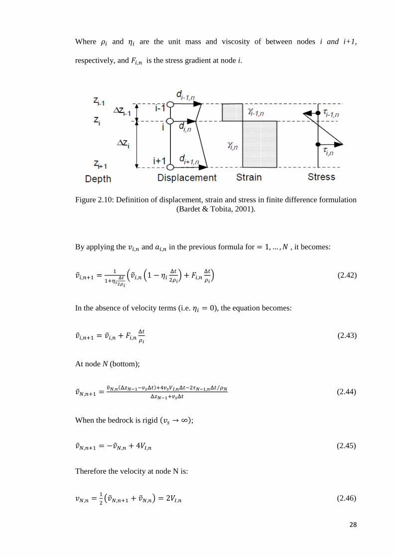
Figure 2.10: Definition of displacement, strain and stress in finite difference formulation

(Bardet & Tobita, 2001). 28

Figure 2.11: Contour map of amplification ratio of Kuala Lumpur for return period of

500 years (Adnan, 2008). 32


2500 years (Adnan, 2008). 33

Figure 2.13: Contour map of acceleration at surface (g) of Kuala Lumpur for the return

period of 500 years (Adnan, 2008). 34

Figure 2.14: Contour map of acceleration of surface (g) of Kuala Lumpur for the return


xiv

Figure 2.15: Contour map of acceleration at surface (g) of Penang for the return period

of 500 years (Adnan, 2008). 36


of 2500 years (Adnan, 2008). 36

Figure 2.17: Contour map of acceleration at surface (g) of Melaka for the return period




Figure 2.19: Contour map of acceleration at surface (g) of Johor Bahru for the return


Figure 2. 20: Contour map of amplification ratio of Johor Bahru for the return period of

500 years (Adnan, 2008). 38

Figure 2.21: Contour map of amplification ratio of Johor Bahru for the return period of

2500 years (Adnan, et al., 2008). 39


period of 2500 years (Adnan, et al., 2008). 39

Figure 3.1: Methodology process. 43

Figure 3.2: Schematic form of a cyclic triaxial cell (Shajarati et al., 2012). 46

Figure 3.3: Stress-strain curve (Phillips et al., 2009). 47

Figure 3.4: Eight point FFT on real input data. 49

Figure 4.1: Program Flowchart. 59

Figure 4.2: Acceleration at bedrock vs. Time (s) plotted by new program code. 60

Figure 4.3: Amplification Ratio obtained from new program code. 61

Figure 4.4: Stress (kPa) obtained from new program code. 61

Figure 4.5: Shear strain (%) obtained from new program code. 62

xv

Figure 4.6: Pseudo Acceleration Spectrum versus Period (sec) obtained from new

program code. 62

Figure 4. 7: Surface Acceleration (g) versus Time (s) Obtained from new program code.

......................................................................................................................................... 63

Figure 4.8: Comparison between Damping Ratio (blue) and G/Gmax (yellow)

calculated by new program code for Clay and Damping Ratio (orange) and G/Gmax

(dark blue) calculated by NERA. 64


calculated by new program code for Sand and Damping Ratio (orange) and G/Gmax

(dark blue) calculated by NERA. 66

Figure 4.10: Comparison between new program code (orange) and NERA (blue) results

for the amplification ratio versus frequency (Hz). 67


for the stress (kPa) versus time (sec). 68


for the strain (%) versus time (sec). 69


for the spectral acceleration versus period. 70

Figure 4. 14: Comparison between new program code (orange) and NERA (blue) results

for the surface acceleration (g). 71

Figure 4.15: The time histories used in ground response analysis for the return period of

500 years. (a) Kuala Lumpur, (b) Penang, (c) Melaka and (d) Johor Bahru. 72

Figure 4.16: Location of boreholes in Kuala Lumpur (Google Earth, 2015). 73

Figure 4.17: Contour map of acceleration at surface of Kl for the return of 500 years. . 76

Figure 4.18: Contour map of amplification factor of Kl for the return of 500 years. 77

Figure 4.19: Location of boreholes in Penang (Google Earth, 2015). 78

xvi

Figure 4.20: Contour map of acceleration at surface of Penang for the return of 500

years. 80

Figure 4.21: Contour map of amplification factor of Penang for the return of 500 years.

......................................................................................................................................... 81

Figure 4.22: Location of boreholes in Melaka (Google Earth, 2015). 82

Figure 4.23: Contour map of acceleration at surface of Melaka for the return of 500

years. 84

Figure 4.24: Contour map of amplification factor of Melaka for the return of 500 years.

......................................................................................................................................... 85

Figure 4 25: Location of boreholes in Johor Bahru (Google Earth, 2015). 86

Figure 4.26: Contour map of acceleration at the surface of Johor Bahru for the return of

500 years. 87

Figure 4.27: Contour map of amplification ratio of Johor Bahru for the return of 500

years. 87

Figure B.1: New program code interface. 122

Figure B.2: The pull-down menu "File". 124

Figure B.3: The pull-down menu "Data". 125

Figure B.4: The pull-down menu "Help”. 126

Figure B.5: Project tab. 127

Figure B.6: Soil profile tab. 128

Figure B.7: Earthquake tab. 128

Figure B.8: Result tab. 129

xvii

LIST OF TABLES

Table 2.1: Strain threshold for cyclic loading (Pecker, 2007). 19

Table 2.2: Characteristic of equivalent linear models (Pecker, 2007). 22

Table 2.3: Site response analysis programs (Bardet et al., 2000; Bardet et al., 2001;

Hashash et al., 2012; Idriss et al., 1992; Redmond; Version). 26

Table 4. 1: Soil material comparison between data obtained from local clay and the one

calculated by NERA. 64


calculated by NERA. 65

Table 4.3: Result of 1-D analysis for KL for the return of 500 years. 74

Table 4.4: Results of 1-D analysis for Penang for the return of 500 years. 79

Table 4.5: Results of 1-D analysis for Melaka for the return of 500 years. 83

Table 4.6: Results of 1-D analysis for Johor Bahru for the return of 500 years. 86

1

CHAPTER 1

INTRODUCTION

1.1 Introduction

Earthquake is the distinguishable movement of the Earth surface, causing from the

unexpected discharge of energy in the Earth's crust that generates seismic waves.

Extreme ground trembling throughout enormous earthquake can destroy or even

damage engineered constructions such as buildings, bridges, highways, and dams.

1.2 Ground Response Analysis

Ground response analysis is to forecast ground surface movement, by using the ground

motion and site soil inspection data, in order to develop the seismic microzonation maps

and to design response spectra, to assess dynamic stresses also strains for assessment of

the liquefaction risks, and to distinguish the seismic forces that cause unsteadiness of

earth also earth sustainable construction. The analysis of the ground response is capable

of modeling the rapture mechanism at the base of a quake, the transmission of stress

waves to top of the bedrock under the particular location, and to decide ground

movements on the surface, in ultimate condition. However, this is a complex process

(Kramer, 1996).

In general, methods for analysing the ground response are grouped dimensionality,

where the arriving shear waves spread from the underlying bedrock. They are one-

dimensional (1-D), two-dimensional (2-D), and three-dimensional (3-D) shear wave

transmission methods. Many of these methods are established on the statement that the

main reactions in a soil deposit are triggered by the ascending propagation of the shear

https://en.wikipedia.org/wiki/Earth

https://en.wikipedia.org/wiki/Crust_(geology)

https://en.wikipedia.org/wiki/Seismic_wave

2

waves that are polarized horizontally (SH waves) from the underground rock foundation

which is shown in Figure 1.1 (Kramer, 1996).

Figure 1.1: Refraction process that produces nearly vertical wave propagation near the

ground surface (Kramer, 1996).

There are several Ground response analysis computer programs used to compute the

earthquake spectra, such as SHAKE, NERA and DEEPSOIL. Some of these programs

are more developed than others based on the numerical methods they apply in the

computer codes.

1.3 Problem Background

According to USGS documentation (Petersen et al., 2007), Southeast Asia is an area of

mutable earthquake threat, oscillating from high earthquake risk related with the

subduction process under the Indonesian and Philippine archipelagos to abstemiously

low earthquake risk across a vast steady region that encloses the Malaysian peninsula.

The earthquake chain surrounded Malaysia is shown in Figure 1.2.

3

Figure 1.2: Map of shallow-depth earthquakes in Southeast Asia (Petersen et al, 2007).

Figure 1.2 indicates the epicentres of shallow-focus seismic activities (focal dept less

than 50 km) for the period 1964-2005 decided by the methodology of Engdahl and other

researchers (Engdahl et al., 1998).

As shown in Figure 1.2 the Malaysian peninsula, western Borneo, and parts of eastern

Thailand are situated inside the stable centre of the Sunda plate and are categorised by

low seismic activity and strain rates. In the boundary of this wide ‘Stable Sunda’ zone,

merely 20 well-located underground eruption with magnitude larger than M5 happened

during the years 1964 to 2007. Geodetic data also signify that strains dignified in this

4

area are low (Rangin et al., 1999b; Simons et al., 2007). This area is located about 300-

600 km away from the Sumatran faults that have caused underground eruption that were

sensed in structures in Singapore and Kuala Lumpur (Brownjohn et al., 2001; Pan,

1997; Pan et al., 1996). The eastern Borneo however, has a reasonable rate of seismic

activity, and geodetic sign of tectonic distortion is testified by Rangin and Simons

(Rangin et al., 1999a; Simons et al., 2007). The major tremor in the zone was the

earthquake of April 19, 1923, with the magnitude of 6.9 (Engdahl et al., 2002).

1.3.1 Problem Statement

The earthquake hazards caused damages in the past years and the further damage is not

predictable. Earthquake does not only cause damage to the structures but to soil

underneath the structures as well. Therefore the stability of soil under structures and the

constancy of the structures built on are in danger. Various soil properties have an impact

on seismic waves as they pass through a soil layer, where tremors may cause the soil

under the structure to shatter and bring the foundations to failure.

Peninsular Malaysia is situated far away from the seismic activity epicentres (the

nearest earthquake epicentre from Malaysia is about 350km), and located in the steady

Sundra Shelf (Adnan et al., 2005). However, quivering due to Sumatra quakes had been

stated numerous times. There were no stark destructions apart from cracks on buildings

in Penang that is stated on 2nd November 2002. Ground response analysis programs are

the tools to calculate the response spectra at the surface or any specific layer in need.

Although the available ground response analysis programs are used to calculate the

response spectrum worldwide, no studies had been taken place on Malaysia’s soil

condition.

5

1.4 Methodology

This study used the previous studies on ground response analysis methods and systems.

Also a computer program code is provided that considered Malaysia’s soil dynamic

properties. The methods applied in this study are presented in Figure 1.3. As it is shown

in the figure the methodology is divided in three sections; Data collection, Data analysis

and Results. Figure 1.3 shows this systematic order in a flow chart.

6

Figure 1.3: Methodology.

7

1.5 Objectives of the Study

The nonlinear site response analysis program which is first launched by Barnet et al

(2001), is not developed as fast as linear programs and it still has some imperfections.

Therefore in this study objectives which mentioned bellow are employed.

1. To develop a seismic site response program code considering local soil dynamic

properties and Newmark is the numerical method.

2. To produce the seismic microzonation map for Kuala Lumpur, Melaka, Penang

and Johor Bahru, by using the developed programming code.

3. To compare the existing seismic microzonation maps and the new ones which

produced in this study, in order to know the effect of different soil material

parameters considered.

1.6 Research Contribution

Since SHAKE90 had launched till now the programs have been improved due to the

need for more details and providing better screening of results. Most of the computer

programs are based on the linear behavior of soil. More developed programs are

calculating the spectra by assuming the soil cyclic behavior that can be simulated by

equivalent linear system. There are few computer programs that compute the data based

on the nonlinear system. Although nonlinear programs have been developed since,

however, to compare with linear systems they still need improvement.

The method used in most ground response analysis programs is 1-D shear wave

propagation method. 1-D shear wave propagation method is established on the theory

that all the boundaries are horizontal and the response of a soil deposit is mostly caused

by shear wave that propagates vertically from underlying bedrock. Furthermore, the

8

length of a layer is vast in comparison to its thickness. Thus it is feasible to model them

as 1-D shear wave propagation horizontal layers.

All these methods are going to be run by applying the C# programming language. The

structure of C# language is very simple, up-to-date, general-purpose and object-oriented

for a software design language. C# language is a proper language to write applications

for both hosted and embedded systems, fluctuating from the very sophisticated

operating systems, down to very small functions. The graphical operator interface of the

C# provides instinctively pleasing views for the management of the program structure

in the large and the different types of individuals. Therefore, the ground response

analysis program would be more user-friendly.

1.7 Scope of Work

The scope of the study is limited to:

Ground response analysis models, which, this study is focused on the nonlinear

model. Also one dimensional wave propagation method is considered for this

study.

Newmark method is applied for the numerical calculation.

Soil material curve presenting G/Gmax and damping ratio versus strain is

proposed.

The program code will be developed by using C# programming language.

Seismic microzonation maps are prepared for 4 main developing cities such as

Kuala Lumpur, Penang, Melaka and Johor Bahru.

9

1.8 Thesis Outline

In order to achieve the objectives, this thesis is organized in six chapters.

Chapter one explains about the basics of the research, introduces the research problems,

objectives of the study and a brief methodology.

Chapter two presents a literature review to indicate the background of the research

context. Therefore, the previous studies, available methods and models provided in

ground response analysis are presented. This is followed by the available computer

programs, the procedure of calculations and their results. The chapter ends by

comparing the mentioned computer program’s results.

Chapter three provides the methods/methodology applied during the research procedure.

The numerical calculations, the soil material curve and program coding are provided in

this chapter.

Chapter four presents the new program prepared by C# programming language and the

data which are analysed with the new program code are demonstrated. The outcomes

and findings are discussed and compared with the available computer programs to check

the accuracy of the new results. Also in this chapter the seismic microzonation maps are

plotted and compared with the available maps.

Chapter five indicates final conclusions, also recommendations that can provide a better

understanding for those who wish to continue this study.

10

CHAPTER 2

LITERATURE REVIEW

2.1 Introduction

Earthquake is one of the most disturbing natural disasters on earth. The tectonic plates

at the Earth’s surface, are constantly moving at the boundaries which will build up large

tectonic stresses that can cause tremors on the surface. Extreme ground shaking, faults

and liquefaction during large earthquakes will lead to damages and even destruction of

engineered structures such as buildings, bridges, highways, and dams (El-Arab, 2011;

Hu et al., 1996; Kamalian et al., 2008; Walling et al., 2009). It is not possible to

intercept earthquakes from happening, however, there is a possibility to moderate the

effects of powerful earthquake shaking and to diminish the casualties and damages. To

predict the ground surface motion earthquake ground response analysis are exerted by

using the ground motion and site soil examination data, for the improvement of design

response spectra, to assess dynamic stresses and strains for evaluation of the

liquefaction hazards, to achieve the microzonation maps, and to distinguish the

pressured force caused by seismic activities that cause the unsteadiness of earth as well

as sustainable structures (Bard, 2000; Field et al., 1995; Fnais et al., 2010; Hu et al.,

1996; Kashani et al., 2017; Kramer, 1996; Mukhopadhyay et al., 2004). Seismic hazard

and microzonation maps of cities enable to distinguish potential seismic areas that need

to be considered when designing structures. The analysis of ground response provides

the fault fracture model at the foundation of seismic activity, the dissemination of stress

waves to top of bedrock under the explicit location, and to launch the ground movement

on the surface, under ultimate condition. However this is a complex procedure.

Microzonation is the course of sub division of an area in to number of zones based on

11

the seismic activity effects in the local scale. Microzonation mapping is to indicate the

estimated response of soil layers under seismic activity excitation. Description and

evaluation of site response throughout earthquake is one of the vital phases of seismic

microzonation in respect to ground trembling intensity, reduction of amplification rate

and liquefaction vulnerability (Farrokhzad et al., 2012; Finn et al., 2004; Grasso et al.,

2009; Hamzehloo et al., 2007; Hendriyawan, 2010).

It is known that the local soil condition can affect the ground response when seismic

waves travel upward through the soil layers, especially for soft clay (Eskişar et al.,

2014; Sun et al., 1988). Effect of site amplification of seismic energy due to soil

condition on destruction was adequately ascertained by many earthquakes during the

past century. Guerrero earthquake (1985) in Mexico city, Spitak earthquake (1988) in

Leninakan, Loma Prieta earthquake (1989) in San Francisco Bay area, Kobe earthquake

(1995), Kocaeli earthquake (1999) in Adapazari and Gujarat-Bhuj earthquake (2001) in

India are the important examples of site amplification (Alpar, 1999; Anbazhagan et al.,

2010; Anderson et al., 1988; Chang et al., 2001; Frankel et al., 1991; Sánchez-Sesma et

al., 1993; Sitharam et al., 2007, 2012; Wyss et al., 1998).

In earthquake engineering practice, site effects are quantified either by theoretical or

empirical models. Theoretical modeling consists performing wave propagation

analyses, which are broadly used to display ground response effects (Hudson et al.,

1994; Idriss et al., 1992). The models for ground response consider nonlinear soil

behavior and encompass a soil domain of limited dimension. Empirical models are

derived from statistical analysis of strong motion data, and quantify the variations of

ground motion across various site conditions. Conceptually, empirical models are

possible if there are many ground motion recordings at the site of interest, but as a

particular matter, such data are seldom available (Stewart, 2008).

12

Nowadays there are several computer programs that convert the input data from the lab

tests to a much understandable spectra by applying different numerical methods or soil

material, which is discussed in the following chapters. In the following sections a

summary on seismic waves, different earthquake response analysis software and their

benefits are provided.

2.2 Seismic Waves

In building structures study of seismic waves comes handy. The science of building

structures is based on several factors, and one of them is soil behavior. Many things can

disturb the soil under the structure, therefore the structure itself, such as seismic waves

(Borcherdt, 1970; Fichtner, 2011; Newmark, 1967; Virieux, 1986).

Seismic waves are divided in two main groups, body waves and surface waves. These

waves are however divided into deferent sections, mainly based on their motion,

velocity and coordination (Stein et al., 2009; Thurber, 2003). These waves are

introduced as follows:

Body waves:

P-Waves, or Primary waves produce displacement in the direction of wave

propagation and cause a volume change. The velocity of these waves are

much higher than other waves (variable from 0km/s and 13km/s) and would

reach the seismometers sooner, therefore they are called primary waves

(Figure 2.1).

S-Waves, or Shear waves propagate in the vertical direction and contort the

material without any volume change. The velocity is much lower than P-wave

(Figure 2.2).

13

Figure 2.1: Schematic form of P-wave propagation (Stein & Wysession, 2003).

Figure 2.2: Schematic form of S-wave propagation (Stein & Wysession, 2003).

Figure 2.1 shows that P-waves compress and dilate the materials on their way. As it

appears in Figure 2.2 S-waves propagate in a sinusoid way with a specified amplitude

and wavelength.

Surface Waves (Kramer, 1996):

Reyleigh Waves, exist near the surface and propagate in a x-z plane (Figure

2.3).

14

Love Waves, propagate near the surface in lower body wave velocity material.

This wave propagates in x-direction with a particle displacement in y-

direction (Figure 2.4).

Figure 2.3: Schematic form of Reyliegh Wave (Stein & Wysession, 2003).

Figure 2.4: Schematic form of Love Wave (Stein & Wysession, 2003).

Figure 2.3 and 2.4 show the complexity of Love and Reyliegh waves along the

propagation.

2.3 One Dimension Earthquake Site Response Analysis

When earthquake happens, body waves move away from the source in every ways. And

when they reach the boundaries between different geological soil layers, the waves

15

reflected and refracted. Because the velocity of wave propagation in shallower material

is lower, the waves are usually imitated to a more vertical course. When the waves

reach the surface, several refractions have bent them to almost a vertical direction

presented in Figure 2.5 (Kramer, 1996).

Figure 2.5: SH wave propagation framework (Midorikawa et al., 1978).

Commonly the methods for evaluating the response of ground motion are grouped

dimensionality, where the inward shear waves spread from bedrock. These are one-

dimensional (1-D), two-dimensional (2-D), and three-dimensional (3-D) shear wave

propagation methods. Many of these methods are based on the theory that the key

responses in a soil deposit are produced by the transmission of horizontally polarized

SH waves moving up from the bedrock foundation.

16

1-D method is based on a supposition that all boundaries are horizontal and that the

response of a soil deposit is primarily produced by SH wave propagating vertically from

bedrock. Although the soil layers sometimes tend to bend, they are considered

horizontal. Moreover, the length of a layer is immeasurable in comparison to its

thickness. Thus it is practical to model them as 1-D horizontal layers. Analytical and

numerical techniques based on this concept, integrating linear approximation to

nonlinear soil behaviour, have shown sensible promises with field testing in many cases

(Hashash et al., 2001; Ishihara et al., 1980; Kramer, 1996).

2.3.1 Ground Response Models

For ground response analysis, transfer function is used to represent different response

parameters, such as displacement, velocity, acceleration, shear stress, and shear strain

and bedrock acceleration. These parameters rely on the principle of superposition

therefore, the proper model is linear systems. However nonlinear behavior can be

resulted approximately, by using an iterative procedure with equivalent linear soil

properties (Kramer, 1996).

Before explaining any models for ground response analysis, here is an explanation to

define the soil behavior under cyclic loading and experimental tests to achieve shear

stress-strain curve.

2.3.2 Soil behavior and shear stress-strain curve under cyclic loading

As described before the horizontal motion is the cause of vertical propagation of

horizontally polarized shear waves. Under this condition a particle of soil is subjected to

stress cycles similar to those shown in Figure 2.6 (Pecker, 2007; Pyke, 1980).

17

Figure 2.6: Stress cycle during earthquake (Pecker, 2007).

When the wave passes through the soil layers a shear stress would apply on the soil

element, and causes a shear strain to be applied as well, which will produce a shear

stress-strain curve as provided in Figure 2.7 (Pecker, 2007).

Figure 2.7: Shear stress-strain curves (Pecker, 2007).

Stress–strain response of soils under cyclic loading is essential for analysing and

designing civil engineering geo-systems. Cyclic loadings will cause transient and

18

permanent deformations in soils which could damage the structures situated on these

soil layers (Basheer, 2002; Shahnazari et al., 2010).

To achieve this curve there are several laboratory tests to find the stress and strain

values, such as; cyclic triaxial shear test, cyclic torsional shear test and simple cyclic

test which are the laboratory test. Here the test functions are introduced.

2.3.2.1 Cyclic Triaxial Test

The most popular method to evaluate the undrained cyclic strength of soil is the cyclic

triaxial test with uniform episodic loading. However, the laboratory stress condition in a

cyclic tiaxial test does not accord to the in situ stress condition in ground level during

earthquake movements. From the output data, stresses and strains are calculated in order

to construct the necessary geotechnical diagrams, and more importantly the hysteretic

loop of the shear stress versus shear strain (Cabalar et al., 2013; Evans et al., 1987;

Kokusho, 1980; Kokusho et al., 1981; Shajarati et al., 2012; Silver et al., 1976).

2.3.2.2 Cyclic Torsional Shear Test

Torsional test apparatus is used in the dynamic deformation characteristics test, in order

to achieve the shear stress-strain relationship, shear modulus and damping ratio versus

shear strain relationship. During the test, constant shear stress amplitude is incremented

from small to large value. Shear modulus and damping ratio are computed from the

hysteresis loop at 10th

cycles of loading in the ordinary loading, but are computed from

the hysteresis loop at the last loading cycle in each stage when amplitude becomes large

(Henke et al., 1993).

19

2.3.2.3 Simple cyclic shear test

The laboratory cyclic undrained simple shear test provides a better stress representation

of the in situ condition in comparison with the cyclic triaxial test (De Alba et al., 1976;

Finn et al., 1971; Peacock et al., 1968). As the horizontal stresses were not measured

nor could be controlled independently of the vertical stresses in these two tests it has

been difficult to compare the test results generated from the simple cyclic shear test and

cyclic triaxial test. Cyclic undrained torsional simple shear test, on the other hand, can

control the horizontal stresses independently of the vertical stresses (Pathak et al.).

During this test the total horizontal stress is kept constant, the vertical strain and the

volumetric strain are zero and the horizontal strain is also zero. This is similar to the in

situ condition in ground level during earthquake movement.

2.3.3 Soil Model Based on Shear Strain threshold

Based on a study on cyclic shear strain identifying the soil behavior model and

therefore, different ground response model, is possible as soon as strain becomes

significant in laboratory test results. In the table below, soil behavior is divided in three

groups based on the strain thresholds for cycling loading and the modeling for each type

of soil is concluded (Pecker, 2008).

Table 2.1: Strain threshold for cyclic loading (Pecker, 2007).

Cyclic Shear Strain γ Behavior Modeling

Very small

Practically Linear Linear

Small

Nonlinear Equivalent Linear

Moderated to large Nonlinear Nonlinear

20

Where is recoverable strain and is irrecoverable strain that develops for larger

thresholds ( to ). The strain threshold when nonlinearity appears is usually

very small ( to ), ( Pecker, 2007).

2.3.3.1 Linear Model

For strains smaller than to ( ) soil behaves elastically. Therefore, the

proper model in this case is linear elastic. Shear modulus G and bulk modulus B

completely describe the model for isotropic materials (Cremer et al., 2002).

(2.1)

(2.2)

Where is shear wave velocity, is dilatational wave velocity and is density

(Pecker, 2007).

A soil deposit of N horizontal layers is considered, where the Nth layer is bedrock

(layered, Damped Soil on Elastic Rock). Every layer of soil acts as a Kelvin-Voigt solid

(The schematic of the Kelvin-Voigt model is shown in Figure 2.8), therefore the wave

equation is (Kramer, 1996):

(2.3)

Figure 2.8: Kelvin-Voigt model (Pecker, 2007).

21

The solution for this equation is expressed as follows:

(2.4)

And shear stress is also given by:

(2.5)

The displacement at the top and bottom of layer m will be:

(2.6)

(2.7)

The transfer function relating to displacement amplitude can be resulted as:

(2.8)

Since the soil behaves in a nonlinear way, the linear system itself is not useful enough,

and needs to be more modified to reach reasonable estimation of ground response

(Kramer, 1996).

2.3.3.2 Equivalent linear

This system, where the strain value is in between the two threshold ( )

consists of modifying the Kelvin-Voigt model. For this model the shear stress-strain

relationship is:

(2.9)

Where G and C are the spring and dashpot coefficients. and are the shear strain and

shear strain rate (Pecker, 2007).

For harmonic loading (Pecker, 2007):

22

(2.10)

In cases of ground response with no soil displacement, the response is mainly based on

the shear modulus and damping characteristics of soil under the cyclic loading.

Therefore, analyses are made by using the equivalent linear method (Seed et al., 1964).

The equivalent linear shear modulus G is taken as a secant shear modulus (Kramer,

1996):

(2.11)

Where is shear stress and is strain amplitude.

The equivalent linear damping ratio, ξ, is the damping ratio that produces the same

energy loss in a single cycle as he hysteresis stress-strain loop of the irreversible soil

behavior (Kramer, 1996).

For this system there are three model assumed based on the studies of Seed and his co-

workers (Seed et al., 1970) and third one is founded by (Leca et al., 1990) These models

are shown in Table 2.2 (Pecker, 2007).

Table 2.2: Characteristic of equivalent linear models (Pecker, 2007).

Model No. Complex Modulus Dissipated Energy in one cycle

Model 1

Model 2

Model 3

There are other models as well, that are described in following chapters. According to

the Table 2.2, in the first model the dissipated energy is duplicated but the stiffness is

overestimated. On the contrast, the second model the stiffness is duplicated, and the

23

dissipated energy is underestimated. However the third model fulfills both conditions

(Pecker, 2007).

As for the computation an iterative process is obligatory to certify that the strain values

used in the analysis are in harmony with computed values in all layers (Kramer, 1996).

2.3.3.3 Nonlinear

In this range ( ) major changes happen in the soil structure. Therefore the

equivalent linear model no longer satisfies the actual nonlinear process of seismic

ground response (Cremer et al., 2001; Kramer, 1996; Pecker, 2008; Pecker et al., 2010).

To analyze the genuine nonlinear response of the soil sediment the use of direct

arithmetic integration is considered in the time domain by integrating the equation of

motion in minor time steps. To do so, the soil layer should be exposed to horizontal

movement at the bedrock level, the response would be as written bellow (Kramer,

1996):

(2.12)

Also the number of soil layers would divided to N sub layers of thickness ΔZ and in

small time increasing of length, Δt , as shown in Figure 2.9.

24

Figure 2.9: Soil layer divided into N sub layers (Kramer, 1996).

Therefore:

(2.13)

(2.14)

Filling these two equations in equation of motion:

(2.15)

Solving this equation for gives:

(2.16)

As the ground surface is a free surface, then , so:

(2.17)

By considering the boundary conditions, the increasing displacement in each time step

is given by:

25

(2.18)

The shear strain in each sub layer is given by:

(2.19)

For the shear stress, though, the computed shear strain, , and the cyclic stress- strain

relationship are used to define the corresponding shear stress , (Kramer, 1996). To

calculate these steps, most nonlinear ground response analysis computer programs use

the explicit formulation, although, this method is unstable numerically if the time step is

too large (Davis, 1986), rather than the implicit finite-difference formulation which,

resolves the constancy problem the explicit method have (Kramer, 1996).

2.4 Earthquake Response Analysis Program

There are several available computer programs used to compute the earthquake spectra,

by using different numerical methods and computer coding. Therefore, some of them

are more developed as compared to others. The most popular programs are SHAKE,

EERA, NERA and DEEPSOIL that summarized in Table 2.3 below and described later

in this chapter.

26

Table 2.3: Site response analysis programs (Bardet et al., 2000; Bardet et al., 2001;

Hashash et al., 2012; Idriss et al., 1992; Redmond; Version).

No Program Producers Description

1 SHAKE Idriss, & Sun,

1992

Linear and equivalent linear 1-D

earthquake site response analysis by using

Windows system.

Based on the continuous solution to the

wave equation (Kanai, 1951).

Applying Fast Fourier Transform

algorithm (Cooley et al., 1965)

Using an iterative procedure.

2 EERA BARDET, et al.,

2000

Linear 1-D earthquake site response

analysis established in FORTRAN 90 and

using Ms. Excel Program.

Using an iterative procedure.

3 NERA BARDET &

TOBITA, 2001

Nonlinear 1-D earthquake site response

analysis established in FORTRAN 90 and

using MS. Excel Program.

Using a nonlinear model known as IM

model describing a nonlinear stress-strain

curve.

Using iterative procedure.

4 DEEPSOIL

Hashash, et al.,

2012

Linear, Equivalent linear and nonlinear 1-

D earthquake site response analysis.

Features an intuitive graphical user

interface.

The equivalent linear analysis mode is

similar to other available codes such as

SHAKE.

The nonlinear model used in this

computer program is based on the MKZ

model.

27

2.5 Numerical Methods to calculate Response Spectrum

There several numerical methods to calculate the response spectrum which available

programs already applied these methods.

2.5.1 Central difference algorithm:

The central difference method is a specific type of Newmark algorithm (Hughes, 1986)

which applied by NERA.

The predicted velocity is:

(2.36)

Where is related to the displacement and velocity at times through:

, (2.37)

(2.38)

Where is the displacement and is the velocity at times and .

As

, therefore velocity and acceleration can be imparted in terms

of predicted velocity at times :

, (2.39)

(2.40)

As it presented in Figure 2.28 strain is constant between nodes i and i+1, which conveys

that the stress is also constant between the nodes. The principal equations at nodes

at time are:

(2.41)

28

Where and are the unit mass and viscosity of between nodes i and i+1,

respectively, and is the stress gradient at node i.

Figure 2.10: Definition of displacement, strain and stress in finite difference formulation

(Bardet & Tobita, 2001).

By applying the and in the previous formula for , it becomes:

(2.42)

In the absence of velocity terms (i.e. ), the equation becomes:

(2.43)

At node N (bottom);

(2.44)

When the bedrock is rigid ;

(2.45)

Therefore the velocity at node N is:

(2.46)

29

which is the result for the rigid rock.

2.5.2 Newmark-beta Method

The Newmark-beta method is a numerical integration method for solving differential

equations. This method is broadly used in numerical evaluation of the dynamic response

of structures and solids such as in finite element analysis to model dynamic systems.

The Newmark method is a family of time stepping methods (Bathe et al., 2012; Chang,

2004; Kane, 1999; Newmark, 1959; Parashar et al., 2013; Rubin, 2007; Zolghadr

Jahromi et al., 2013). By using the extended mean value theorem, the Newmark β

method expresses that the first time derivative (velocity in equation of motion) can be

solved as:

(2.47)

Where,

(2.48)

Therefore,

(2.49)

Due to changing acceleration in time, the extended mean value theorem must also be

extended to the second time derivative to capture the correct displacement,

(2.50)

(2.51)

Where reasonable value of is .

Therefore the updated rules are:

http://en.wikipedia.org/wiki/Differential_equations

http://en.wikipedia.org/wiki/Differential_equations

http://en.wikipedia.org/wiki/Finite_element_analysis

30

(2.52)

(2.53)

The parameters β and γ define the variation of acceleration over a time step and

determine the stability and accuracy of the method. These two equations combined with

the equilibrium equation of motion at the end of the time step, providing the basis for

computing at time i+1.

2.6 Seismic Microzonation Map

The drill of seismic engineering includes the discernment and modification of seismic

risks. Microzonation is the accepted tool in seismic hazard evaluation and risk

estimation and it is outlined as the zonation with respect to ground motion

characteristics of the source and site conditions (Pelekis et al., 2013; The Technical

Committee for earthquake geotechnical engineering, 1999; Turk et al., 2012); Ishihara,

1993). Microzonation of an area provides detailed maps that forecast the risk at a

smaller scale. Seismic microzonation is the general description for subdividing a region

into distinct areas with variety of potential harmful earthquake effect, describing their

explicit seismic actions for engineering scheme and also land-use planning

(Lamontagne et al., 2011; Lee et al., 2015; Marto et al., 2011; Mohanty et al., 2009;

Mukhopadhyay et al., 2004; Murvosh et al., 2013; Purnachandra Rao et al., 2011). The

role of geological and geotechnical data become significant in the microzonation,

especially in the planning of city urban infrastructure, which can recognize, control and

prevent geological hazards for applications in planning of the city infrastructure (Ansal

et al., 2010; Bell et al., 1987; Dai et al., 2001; Farrokhzad et al., 2012; Fuchu et al.,

1994; Hake, 1987; Rau, 1994). The basics of microzonation are to model the rupture

mechanism at the source of the earthquake, approximate the wave propagation through

31

the earth and to the top of the bed rock, and define the effect of soil profile and so to

develop a hazard map designating the susceptibility of the area to possible seismic risk.

Seismic microzonation is helpful in planning buried lifelines such as tunnels, water and

sewage lines, gas and oil lines, and power and communication lines. Seismic

microzonation maps also address the seismic activity characteristic and local geological

site condition and generally it is the course of assessing the reaction of soil layers for

earth incitement and therefore, the discrepancy of underground eruption characteristic is

implied on surface (Sitharam et al.).

Cities that are growing rapidly with increasing populations are in need of the

development of new residential areas. Hence, city planning comes to be an important

concern (Bahrainy, 1998; Bell, 1998; De Mulder, 1996; Grasso et al., 2009; Kolat et al.,

2012; Topal et al., 2003). In city planning to govern and avoid geological hazards the

geological and geotechnical data are playing an important role (Bell et al., 1987; Dai et

al., 2001; Hake, 1987; Legget, 1987; Rau, 1994; Van Rooy et al., 2001). Cities that are

rapidly developing can take advantage from the seismic microzonation studies (Finn et

al., 2004). The input data provided in this study can be used in seismic design, land use

management, also approximation of possible liquefaction and landslides. Moreover it

delivers the basics for approximating and plotting the probable destruction to structures

(Anbazhagan et al., 2010; Mukhopadhyay et al., 2004; Satyam et al., 2008; Sharafi et

al., 2009).

Seismic microzonation maps have been prepared for several developing cities in

Malaysia such as Kuala Lumpur, Penang, Melaka and Johor Bahru (Adnan, 2008). Site

response analysis results were used to plot the contour maps of surface acceleration and

amplification factor for the return period of 500 and 2500 years. The developed map are

presented by using GIS (Geographic information system).

32


500 years (Adnan, 2008).

33



34

Figure 2.13: Contour map of acceleration at surface (g) of Kuala Lumpur for the return

period of 500 years (Adnan, 2008).

35

Figure 2.14: Contour map of acceleration of surface (g) of Kuala Lumpur for the return


36


of 500 years (Adnan, 2008).



37





38



Figure 2. 20: Contour map of amplification ratio of Johor Bahru for the return period of


39

Figure 2.21: Contour map of amplification ratio of Johor Bahru for the return period of

2500 years (Adnan, et al., 2008).


period of 2500 years (Adnan, et al., 2008).

In order to plot the microzonation maps there are several soft-wares available, such as

Surfer and GIS.

Surfer is a software package for Windows, which displays data to create base maps,

contour maps, post and classed post maps, image maps and other maps. Surfer provides

the facility for calculating the area and length, also calculating volumes. It also can

40

create profiles (Bresnahan et al., 2002).To prepare a base map Surfer gives the ability to

import an available base map and allows to use the map coordinates in the file for the

imported base map. The Imported map can be geo-referenced in which the image will

be imported in correct real world coordinates. Surfer usually is used in topography and

to plot the topographic maps. The maps are in 2D or 3D version in different types and

methods to provide a better understanding of the earth surface.

GIS (Geographic Information System) is a system of computer software, hardware and

data that make it possible to analyze, and present information which is tied to a location

on the earth’s surface (Dai et al., 2001; Turk et al., 2012). GIS software provides

functions and tools needed to input and store geographic information (Chang, 2006;

Jenson et al., 1988). All GIS software packages rely on an underlying database

management system (DBMS) for storage and management of the geographic and

attribute data. The GIS communicates with the DBMS to perform queries specified by

the user.

One of the greatest advantages of using GIS is its capacity to combine layers of data

into a single map. GIS can be used to explain events, planning strategies, integrate

information, solve complicated problems, predict outcomes, create smart maps and etc.

GIS is usually used in planning strategies, environmental engineering, local and federal

Government, transportation and many other fields (Longley et al., 2001).

2.7 Concluding Remarks

All these programs that have been published in past years were developed- either by

mathematical formulations or programming concepts- in order to achieve results with

more exact details. However this developing process still continues.

41

One of the main problems available programs have is that the calculations are based on

the soil dynamic properties obtained from different part of the world. This may cause

the results not to be exact. With growing knowledge of soil and cyclic behaviour of soil

under earthquake vibrations the previous programs need to be developed. Therefore,

this new program will be a solution by applying C# to make a more user friendly

program, and is based on the Malaysia’s soil condition.

Microzonation maps provide a better understanding of the ground surface acceleration

effects on structures by plotting the amplification values calculated from borehole data

on the specified co-ordinations.

42

CHAPTER 3

METHODOLOGY

3.1 Introduction

This chapter describes the methods applied in this project to answer the research

problems and to achieve the objectives. The methodology utilized in this research is

related and guided by the theoretical approach defined in Chapter two. The three main

approaches are the numerical process, the computer programming and plotting the

microzonation maps. Site response analysis methods can be categorized in three main

sections; the model utilized as linear, equivalent-linear and nonlinear, the domain in

which the calculations are executed, frequency or time domain. Also the dimensionality

of the space in which the analysis is accomplished, 1-D, 2-D and 3-D.

The model selected for this research is the nonlinear model. Nonlinear ground response

analysis provides more precise characterization of nonlinear behavior of soil. The

nonlinear systems are time domain based, where the calculation is done according to the

time steps. The dimensionality of the space chosen to be used in this research is 1-D

method rather than 2-D or 3-D methods. The 1-D time domain analysis is performed by

pursuing a finite difference method. The general view of the methods is divided into

three categories; Data collection, Analysis and Results. In Figure 3.1 the process of the

research is shown and described later.

43

Figure 3.1: Methodology process.

3.2 Data Collection

Data and information which will be used in the research process are provided as:

3.2.1 Earthquake Data Collection

Earthquake data collection for all states in Malaysia: Earthquake data, such as time

history and response spectrum at bedrock of Malaysia had been produced by some local

researchers (Adnan, 2013; Razak et al., 2013). The data will be collected as an input for

the ground response analysis.

Results

Microzonation Map Visual Basic Programming

Result Comparison

Analysis

Analysis Method Reference Curves Numerical Calculations

Data Collection

Earthquake Data Collection Soil Material

44

3.2.2 Soil Material

Soil borehole data - including soil type, thickness of layer H, unit weight ρ, shear

modulus G and shear wave velocity properties - are collected by operating the NSPT

tests on local soil of Kuala Lumpur, Penang, Melaka and Johor Bahru, using the help of

government bodies and private companies to obtain this data. The soil data were then

analysed using the cyclic triaxial cell to obtain the soil material curves such as G/Gmax

and damping ratio versus strain.

3.3 Analysis

This section contains the numerical calculations and programming. Therefore the

collected data were analysed and the methods and formulations that has been studied

were applied.

3.3.1 Analysis Methods

In order to solve the equation of motion in this program the one-dimensional (1-D)

shear wave propagation method was adopted in a nonlinear hysteretic medium in the

time domain. As described in previous chapter the reasons to choose this method are;

1-D shear wave propagation method is based on the assumption that all

boundaries are horizontal and,

The length of a layer is infinite in comparison with its thickness,

Therefore it is practical to model them as 1-D horizontal layers. The soil under different

strain level behaves linearly or nonlinearly. The nonlinear behaviour of the soil during

the cyclic loading is the main point of this research, thus the nonlinear system has been

chosen for the numerical part of the project. The dynamic equation is solved in the time

domain;

45

(3.1)

Where [M] is the mass matrix, [C] is viscous damping matrix and [K] is nonlinear

stiffness matrix. are the displacement, velocities, and acceleration of

the mass [M] relative to the base respectively. is the acceleration of the base. The

damping in the soil can be obtained from the hysteretic loop.

The Nonlinear approach is the main study of this research which contains several steps:

In the nonlinear process at the beginning of each time step the total displacement

and particle velocity are known at each boundary; Particle velocity,

(3.2)

The particle displacement ( profile is used to define the shear strain

within each layer;

(3.3)

(3.4)

The stress strain relationship is used to determine the shear stress in each

layer;

(3.5)

The input motion is used to decide the motion at the base of the soil layer at time

.

The motion of each layer boundary at time is analysed from bottom to

top.

The process is repeated from the beginning to calculate the response in the next time

step.

46

3.3.2 Soil Material

G/Gmax-strain curve, damping-strain curve and stress-strain curve is achieved for

Malaysia’s soil dynamic properties. This is accomplished experimentally and

numerically.

Experimental: To gain the strass-strain curve and damping-strain curve a

laboratory test has been chosen. The Cyclic Triaxial Test is to determine the

stress and strain values of a soil specimen in order to plot the stress-strain curve.

Figure 3.2 presents a close-up of the cyclic triaxial cell. The experiment on 2

types of soil is done by other researchers in Malaysia which is considered in this

research.

Figure 3.2: Schematic form of a cyclic triaxial cell (Shajarati et al., 2012).

Numerical: In order to plot these curves, the data collected in the previous

section were needed. As this research is based on the nonlinear behaviour of the

47

soil, the formulae’s acceptable for this category are chosen from the nonlinear

system. The shear strain were achieved from the formula below:

(3.6)

The shear stress which is obtained from Masing rules is as follows:

(3.7)

(3.8)

The Damping ratio is calculated from the cyclic stress-strain curve plotted by the

stress and strain values obtained from equations above, and used to plot the

respective curve.

According to Figure 1.4 the damping ratio can be calculated as;

(3.9)

Where A and B are areas of the stress-strain curve specified in Figure 3.3.

Figure 3.3: Stress-strain curve (Phillips et al., 2009).

48

3.3.3 Numerical Calculations

The step by step numerical calculation of Bedrock time history is described in two main

sections; FFT Calculations and Response Spectrum Analysis which is based on

Newmark’s method.

FFT Calculations

The collected time histories and response spectrum at bedrock will be scaled and

filtered to suit the targeted location. This is done by applying Fourier series. The

Fourier series for an arbitrary function of time specified over the interval

–

is :

(3.10)

The Fourier series break down into a sum of Fourier terms. To express the

Fourier series for a given function the coefficients, and need to be solved:

(3.11)

(3.12)

(3.13)

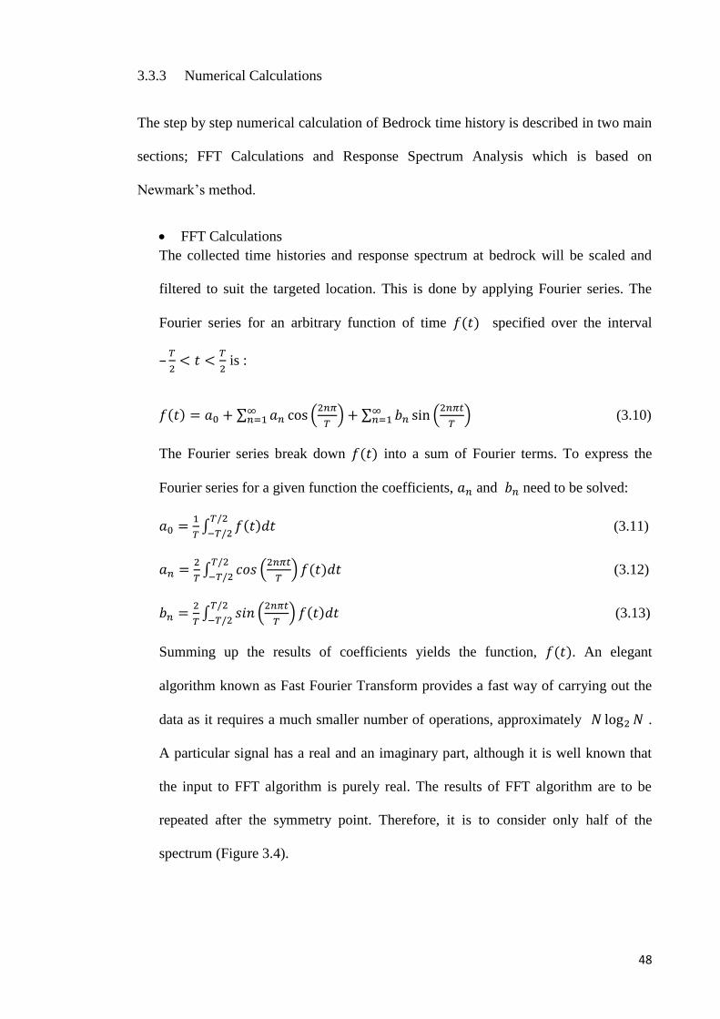
Summing up the results of coefficients yields the function, . An elegant

algorithm known as Fast Fourier Transform provides a fast way of carrying out the

data as it requires a much smaller number of operations, approximately .

A particular signal has a real and an imaginary part, although it is well known that

the input to FFT algorithm is purely real. The results of FFT algorithm are to be

repeated after the symmetry point. Therefore, it is to consider only half of the

spectrum (Figure 3.4).

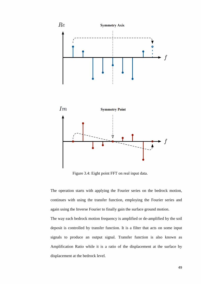
49

Figure 3.4: Eight point FFT on real input data.

The operation starts with applying the Fourier series on the bedrock motion,

continues with using the transfer function, employing the Fourier series and

again using the Inverse Fourier to finally gain the surface ground motion.

The way each bedrock motion frequency is amplified or de-amplified by the soil

deposit is controlled by transfer function. It is a filter that acts on some input

signals to produce an output signal. Transfer function is also known as

Amplification Ratio while it is a ratio of the displacement at the surface by

displacement at the bedrock level.

50

Transfer function is achieved by below formulae’s for layered damped soil on

elastic rock:

For any layer (j) the displacement function is:

(3.14)

From equilibrium;

(3.15)

From compatibility;

(3.16)

, (3.17)

Therefore the transfer function will derived as:

(3.18)

Response Spectrum Analysis

The Response Spectrum analysis is to achieve the Acceleration, Velocity and

Deformation Spectrum. However to calculate the Spectral ordinates a nonlinear

numerical method such as Newmark-beta is considered in this research.

Basically Newmark-beta method for nonlinear analysis provide step by step

calculations to achieve the peak deformation, in order to use the results to proceed

with response spectrum analysis. The full description of the method is in Table 3.1.

The full description for this method is available in Dynamics of Structures by

Chopra in 1995.

51

Table 3.1: Newmark’s method: Nonlinear systems (Average acceleration method) without

iteration (Chopra, 1995).

Average acceleration method:

1.0 Initial calculation

1.1

1.2 select

1.3

and

2.0 Calculation for each time step, i.

2.1

2.2 Determine the tangent stiffness

2.3

2.4

2.5

2.6

2.7

3.0 Repetition for the next time step. Replace i by i+1 and implement step 2.1 to 2.7.

52

After calculating the peak deformation the value can be used to calculate the

response ordinates, which are; displacement (D), pseudo velocity (V) and

pseudo acceleration spectra (A). These functions are based on the natural

frequency (ω) or period (T). The peak value of the displacement spectrum (D) is

determined from the deformation history, which calculated in the previous

section,

(3.19)

in which is the maximum value of the deformation.

Pseudo velocity and acceleration spectrum with natural frequency ω are related

to their peak deformation value and indicates:

(3.20)

(3.21)

3.4 Results

The results of this research are divided into three sections; the first is to plot the

microzonation maps by using the soil information from borehole data, after ensuring

and testing the methods for calculation the nonlinear response analysis program is

produced by taking advantage of C# language and at the end of the process the new

program will be evaluated.

3.4.1 Seismic Microzonation Map

Seismic microzonation maps in this research are plotted for four cities in Malaysia;

Kuala Lumpur, Penang, Melaka and Johor Bahru. For each city 10 to 37 boreholes are

tested. The data needed for the process are specified in coordination of the boreholes in

different areas of each city and the amplification data - which indicates the amplified

53

acceleration on the ground surface – calculated from the soil profile data, bedrock and

ground surface acceleration. The collected data from boreholes are calculated via the

new program code which results the amplification values needed for mapping.

3.4.2 C# Programming

The C# language is a multi-paradigm programming language encompassing strong

typing, imperative, declarative, functional, generic, object-oriented (class-based) and

component-oriented programming disciplines. It was developed by Microsoft within its

.NET initiative and later approved as a standard by ECMA (ECMA-334) and ISO

(ISO/IEC 23270:2006). C# is one of the programming languages designed for Common

Language Infrastructure. Its development team is led by Anders Hejlsberg.

3.4.3 Result Comparison

The acceleration at the surface and the spectral acceleration for the new earthquake

ground motion analysis will be compared with the existing program to verify the

analysed result. This will be done by computer program such as NERA.

54

CHAPTER 4

RESULTS AND DISCUSSION

4.1 Introduction

The three objectives of current study were to develop a local seismic site response

program code based on local soil dynamic properties, to produce seismic microzonation

maps for four cities in Malaysia and to compare the existing maps with the new ones to

understand the effect of different parameters. In this chapter the research findings and

results, the numerical methods, the graphs as the result of running the program code and

seismic microzonation maps are discussed, compared and analysed.

4.2 The seismic ground response analysis

A nonlinear ground response analysis program contains three main sections; Input data,

soil material section and response spectrum. The first section, input data is where the

user can easily insert the necessary information. Such as earthquake time history at

bedrock and the soil data obtained from NSPT tests, including the number of layers, soil

type, shear wave velocity and thickness of each layer. In soil material section the shear

moduli, the ratio between the shear moduli and the maximum shear moduli and the soil

damping ratio are calculated and plotted.

The rest of the procedure is the calculating the numerical methods step by step to

achieve the response spectrum. For the second and third part of the analysis procedure,

soil material and the response spectrum, there are different calculation methods which

we chose the ones that were suitable for this study.

55

4.3 Generating the FFT Calculation

The Fast Fourier Transform (FFT) is an elegant algorithm providing a fast way to carry

out the data processing, as it requires a much smaller number of operations

approximately . The analysis of seismic data using FFTs requires computers.

Thus the ground motion which is a continuous function of time, goes through a number

of analysis steps to finally result the Amplification factor and the acceleration at the

surface. The step are summarised as follows:

1. Input time history of the bedrock motion.

2. First FFT applies.

3. Transfer function calculates the amplification factor.

4. Second FFT applies.

5. Applying the inverse FFT presents the time history of the ground surface motion.

The procedure of the calculation of the third step is described in the following section.

4.3.1 Input data

The soil data obtained from the boreholes in the investigated site are five parameters for

each layer:

1. Thickness (h), [m];

2. Shear wave velocity (Vs), [m/s];

3. Density ( ), ;

4. Attenuation value (β),

5. Number of layers, including half-space (bedrock).

56

4.3.2 Procedure of the Transfer Function Calculation

This procedure is divided into three sections;

1. The shear modulus (G) for all layers is calculated:

(4.1)

Where is density, is shear wave velocity and j indicates the number of layers.

2. Three complex parameters need to be calculated;

a. Complex Shear Module (G*):

(4.2)

Where G is shear module (Eq. (1)), β is attenuation value from input data, and i

is imaginary unite.

b. Complex Impedance Ratio ( ) between layers j and j+1:

(4.3)

c. Temporary Complex variable ( ):

(4.4)

Where is density, is complex shear module and j is number of layers.

3. Process of calculating the transfer function (TF).

Transfer function depends on the frequency therefore, the frequency step, , needs to

be calculated. The calculation is with respect to the acceleration.

(4.5)

Where n is the number of input data for the acceleration and is the time step.

57

The next step is to find the temporary complex variable ( ) number therefore, the round

frequency ( ) and complex wave number (K) need to be calculated.

(4.6)

Where, is the frequency step.

(4.7)

Where K is the complex wave number. The temporary complex variable ( ) is

calculated with the following equation:

(4.8)

Where is thickness of layer from the input data.

Calculation of the amplitudes of up and down direction A and B respectively:

(4.9)

(4.10)

This algorithm starts at the top of the free surface, where there is no shear stress,

therefore:

The transfer function concerning the displacement amplitude at layer i to layer j is

calculated by:

(4.11)

This equation also defines the amplification of acceleration from each two different

layer. The source text of MATLAB codes for this section is available in Appendix A for

the computation of the analytical transfer function as explained above.

58

4.4 Program Flowchart and Results

A computer program is a list of instructions that guide the user through the data analysis

and results. It contains step by step guidelines, commands and finally it provides the

results, which can be presented as graphs or numbers, depends on what the user

requested.

The Nonlinear Earthquake Site Response Analysis program is to provide the response

spectra on the earth surface by calculating the soil input data and time history of the

bedrock. The step by step procedure of this program is presented in the flowchart

(Figure 4.1).

The results of running this program for a set of input data have been presented step by

step in this section.

59

Data Collection

Input data:

Bedrock time

history

Soil material

Calculate:

G

ξ

G/Gmax

Calculate FFTs for bedrock

motions

Plot the results

Plot the results

Get surfer motion

from FFT results

Choose Tn and ξ

Calculate Newmark’s

method

Choose u0

Calculate response

spectrum

End

Plot the results

End

Figure 4.1: Figure 4.1: Program Flowchart.

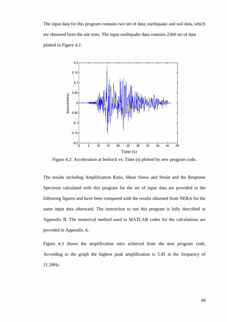
60

The input data for this program contains two set of data; earthquake and soil data, which

are obtained from the site tests. The input earthquake data contains 2360 set of data

plotted in Figure 4.2.

Figure 4.2: Acceleration at bedrock vs. Time (s) plotted by new program code.

The results including Amplification Ratio, Shear Stress and Strain and the Response

Spectrum calculated with this program for the set of input data are provided in the

following figures and have been compared with the results obtained from NERA for the

same input data afterward. The instruction to run this program is fully described in

Appendix B. The numerical method used in MATLAB codes for the calculations are

provided in Appendix A.

Figure 4.3 shows the amplification ratio achieved from the new program code.

According to the graph the highest peak amplification is 5.45 at the frequency of

21.39Hz.

Time (s)

61

Figure 4.3: Amplification Ratio obtained from new program code.

The following graphs show the shear stress and shear strain and spectral acceleration

and surface acceleration resulted via running the new program code. Figure 4.4

illustrates the Shear stress versus time. As it is shown in the graph the highest value of

shear stress is 0.31kPa.

Figure 4.4: Stress (kPa) obtained from new program code.

62

Figure 4.5 is presenting the shear strain versus time. The graph shows that the highest

peak of shear strain is recorded at 89 second which is 0.0029%.

Figure 4.5: Shear strain (%) obtained from new program code.

Figure 4.6 shows the results for Spectral Acceleration versus period. The highest value

is calculated 1.75g on period of 0.07 second.

Figure 4.6: Pseudo Acceleration Spectrum versus Period (sec) obtained from new

program code.

63

Figure 4.7 is presenting the acceleration on the ground versus time. As it is shown in the

graph the peak acceleration obtained from new program code is 0.097g.

Figure 4. 7: Surface Acceleration (g) versus Time (s) Obtained from new program code.

4.4.1 Result comparison

The same set of input data have been ran in NERA in order to check and compare the

results. The graphs provided in the following figures are a comparison between the

outcomes resulted in new program code and NERA.

Table 4.1 is showing the local clay material compared with the soil material calculated

by NERA for the same type of soil. Damping ratio and G/Gmax obtained for the local

clay of Malaysia and soil materials calculated by NERA for the same type of soil are

presented.

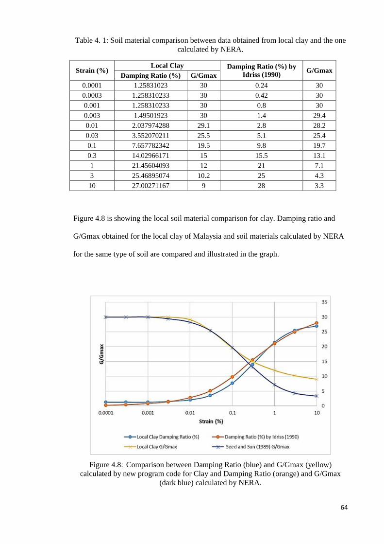
64


calculated by NERA.

Strain (%) Local Clay Damping Ratio (%) by

Idriss (1990) G/Gmax

Damping Ratio (%) G/Gmax

0.0001 1.25831023 30 0.24 30

0.0003 1.258310233 30 0.42 30

0.001 1.258310233 30 0.8 30

0.003 1.49501923 30 1.4 29.4

0.01 2.037974288 29.1 2.8 28.2

0.03 3.552070211 25.5 5.1 25.4

0.1 7.657782342 19.5 9.8 19.7

0.3 14.02966171 15 15.5 13.1

1 21.45604093 12 21 7.1

3 25.46895074 10.2 25 4.3

10 27.00271167 9 28 3.3

Figure 4.8 is showing the local soil material comparison for clay. Damping ratio and

G/Gmax obtained for the local clay of Malaysia and soil materials calculated by NERA

for the same type of soil are compared and illustrated in the graph.


calculated by new program code for Clay and Damping Ratio (orange) and G/Gmax

(dark blue) calculated by NERA.

65

As presented in Figure 4.8 the graph is plotted for damping ratio and G/Gmax versus

strain (%). Damping ratio which is calculated by new program code is close to the trend

of calculated damping ratio by NERA. However, the difference between the damping

values are significant from 0.01% to 0.3%. The difference between local clay damping

ratio and the damping ratio calculated by NERA is approximately around 27%. While

the difference between G/Gmax values obtained for local clay and NERA from 0.3% t0

10% strain is around 3%.

Local sand material and the soil material calculated by NERA for the same type of soil

are compared. Damping ratio and G/Gmax obtained for the local sand of Malaysia and

soil materials calculated by NERA for the same type of soil are presented in Table 4.2.


calculated by NERA.

Strain (%) Local Sand Damping Ratio (%)by

Idriss (1990) G/Gmax

Damping Ratio (%) G/Gmax

0.0001 1.258310233 30 0.24 30

0.0003 1.258310233 30 0.42 30

0.001 1.381192293 30 0.8 29.7

0.003 1.772526775 28.2 1.4 28.8

0.01 3.498586413 22.6 2.8 25.5

0.03 8.064336054 16.9 5.1 19.2

0.1 16.38492215 10.2 9.8 11.1

0.3 23.89261402 6.9 15.5 5.4

1 28.39233141 5.1 21 2.4

3 29.81598361 4.5 25 1.5

10 30.54057188 3.3 28 1.05

Figure 4.9 is presenting the local soil material comparison for sand. Damping ratio and

G/Gmax obtained for the local sand of Malaysia and soil materials calculated by NERA

for the same type of soil are compared and shown in the graph below.

66


calculated by new program code for Sand and Damping Ratio (orange) and G/Gmax

(dark blue) calculated by NERA.

According to Figure 4.9 from 0.01% to 10% of strain values the difference between the

local sand damping ratio and the damping ratio calculated in NERA is almost around

24%. While the difference between G/Gmax values from 1% to 10% of strain is

approximately around 11%.

Figure 4.10 shows the comparison between calculated amplification ratio by NERA and

the new program code.

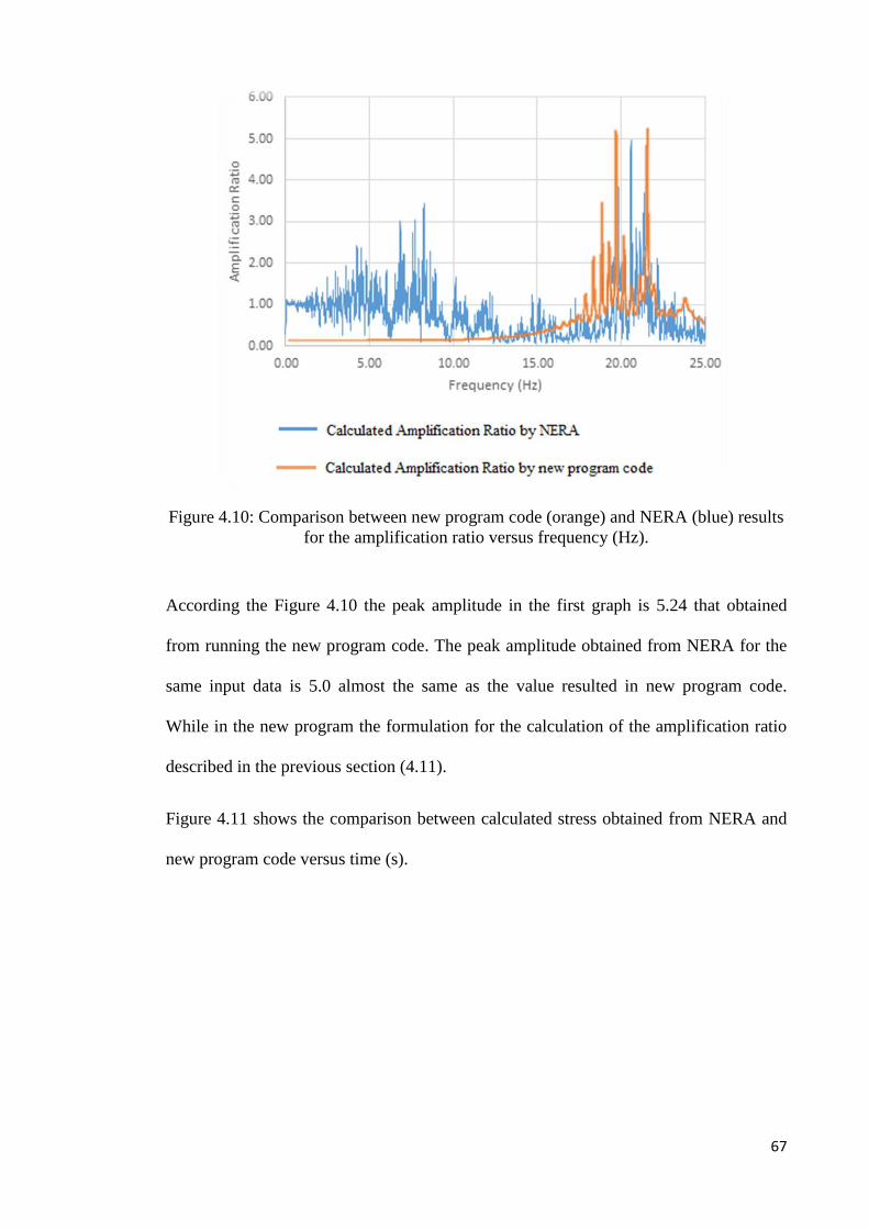
67


for the amplification ratio versus frequency (Hz).

According the Figure 4.10 the peak amplitude in the first graph is 5.24 that obtained

from running the new program code. The peak amplitude obtained from NERA for the

same input data is 5.0 almost the same as the value resulted in new program code.

While in the new program the formulation for the calculation of the amplification ratio

described in the previous section (4.11).

Figure 4.11 shows the comparison between calculated stress obtained from NERA and

new program code versus time (s).

68


for the stress (kPa) versus time (sec).

The shear stresses shown in the graph above are calculated in new program code and

NERA for same set of input data. The peak stress obtained from new program code is

lower by 0.31 (kPa) where the peak stress gained from NERA is at 0.37 (kPa).

Figure 4.12 presents the shear strain calculated by NERA compared to the calculated

shear strain by new program code versus time (s).

69


for the strain (%) versus time (sec).

According to Figure 4.12 for same set of input data the peak strain obtained from new

program code is 0.0027 and the peak from NERA is 0.0026.

Figure 4.13 is the comparison between new program code and NERA for the spectral

acceleration versus period.

70


for the spectral acceleration versus period.

The spectral acceleration outcomes resulted from different methods of calculation are

described in Chapter 2. NERA applied Central Difference algorithm to calculate the

response spectrum, while we applied Newmark method which is known to have more

exact results in time domain for nonlinear analysis. As it shown in the first graph,

Figure 4.13, the peak spectral acceleration is 1.7491 and the result from NERA analysis

shows that the peak spectral acceleration is 1.89.

Figure 4.14 is presenting the comparison between surface acceleration obtained by the

new program and NERA. According to Figure 4.14 the peak acceleration obtained from

new program code is 0.097 (g) where the peak acceleration gained from NERA is at

0.073 (g).

71

Figure 4. 14: Comparison between new program code (orange) and NERA (blue) results

for the surface acceleration (g).

4.5 Seismic Microzonation maps

The most developing cities in Malaysia are selected for the seismic microzonation

studies; Kuala Lumpur, Penang, Melaka and Johor Bahru. To accomplish the peak

acceleration and the amplification factor at surface shear wave transmission analyses

were performed for all the existing soil data in the mentioned cities. One time history is

used in this study which is the return period of 500 years for each city. This time history

is reported by Engineering Seismology and Structural Earthquake Engineering Research

(e-SEER), University Technology Malaysia (Adnan, 2013). The soil data gained from

borehole testing is calculated with the new program code. The results containing the

amplification factor attained from the new program code is used in plotting the seismic

microzonation maps. In order to plot the maps three sets of data are applied in Surfer

11; Coordination of each borehole (longitude and latitude) and also amplification factor.

The time history of each city for the return period of 500 years is shown in Figure 4.15.

72

Figure 4.15: The time histories used in ground response analysis for the return period of

500 years. (a) Kuala Lumpur, (b) Penang, (c) Melaka and (d) Johor Bahru.

Numerous soil data is collected for this study from various sites in Kl, Penang, Melaka

and Johor Bahru. For each data, the soil dynamic properties were achieved via altering

the static factors of NSPT values and using the nonlinear response analysis method for

the calculation done in the new program code. The results of acceleration, amplification

factor at the surface and the seismic microzonation maps are provided in the following

subchapters.

4.5.1 Kuala Lumpur

Kuala Lumpur, situated midway along the west coast of Peninsular Malaysia, is one of

the most developing cities in Malaysia. Soil data gained from NSPT tests scattered in

the city indicates that the dominate soil types are silt and clay. The location of boreholes

are shown in Figure 4.16. Number of boreholes, location of boreholes, acceleration at

bed rock and surface, amplification factor are provided the in Table 4.3 and 4.4.

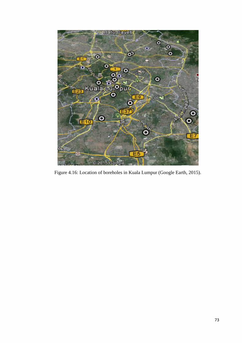
73

Figure 4.16: Location of boreholes in Kuala Lumpur (Google Earth, 2015).

74

Table 4.3: Result of 1-D analysis for KL for the return of 500 years.

Number

of

Boreholes

Location of Boreholes Acceleration

Amplification

Factor Latitude Longitude Bedrock Surface

1 3.175 101.676 0.065 0.223 3.40

2 3.176 101.676 0.065 0.141 2.15

3 3.147 101.689 0.065 0.12 1.83

4 3.147 101.690 0.065 0.941 14.38

5 3.180 101.702 0.065 0.210 3.22

6 3.153 101.701 0.065 0.491 7.52

7 3.137 101.679 0.065 0.203 3.10

8 3.136 101.678 0.065 0.437 6.68

9 3.078 101.710 0.065 0.401 6.13

10 3.079 101.711 0.065 0.219 3.34

11 3.160 101.684 0.065 0.598 9.14

12 3.161 101.683 0.065 0.576 8.80

13 3.085 101.632 0.065 0.279 4.26

14 3.084 101.634 0.065 0.266 4.06

15 3.140 101.692 0.065 0.629 9.61

16 3.139 101.691 0.065 0.473 7.23

17 3.093 101.683 0.065 0.264 4.03

18 3.094 101.681 0.065 0.222 3.39

19 3.181 101.706 0.065 0.156 2.38

20 3.183 101.708 0.065 0.1 1.52

21 3.058 101.692 0.065 0.201 3.07

22 3.059 101.691 0.065 0.178 2.72

23 3.098 101.747 0.065 0.119 1.81

24 3.097 101.746 0.065 0.169 2.58

25 3.195 101.744 0.065 0.244 3.73

75

Table 4.3: Result of 1-D analysis for KL for the return of 500 years (continued).

Number

of

Boreholes

Location of Boreholes Acceleration Amplificatio

n factor Latitude Longitude Bedrock Surface

26 3.194 101.744 0.065 0.169 2.58

27 3.141 101.727 0.065 0.614 9.38

28 3.204 101.736 0.065 0.381 5.82

29 3.203 101.737 0.065 0.149 2.27

30 3.111 101.700 0.065 0.227 3.47

31 3.113 101.697 0.065 0.263 4.02

32 3.110 101.703 0.065 0.168 2.56

33 3.112 101.700 0.065 0.125 1.91

34 3.113 101.697 0.065 0.1 1.52

35 3.114 101.695 0.065 0.227 2.87

36 3.117 101.692 0.065 0.188 3.40

37

3.120 101.690 0.065 0.096 3.47

According to the table above the amplification factors show the ratio between

acceleration at bedrock and at surface. Seismic microzonation maps indicate

acceleration at surface and amplification factor in Kuala Lumpur for the return of 500

years are shown in Figures 4.17 and 4.18 respectively.

76

Figure 4.17: Contour map of acceleration at surface of Kl for the return of 500

years.

77

Figure 4.18: Contour map of amplification factor of Kl for the return of 500 years.

Figure 4.17 shows the contour maps of surface acceleration of Kuala Lumpur on the

areas that the soil data had been collected. While figure 4.18 presents the contour maps

of amplification factor. As it seems in the acceleration contour map, the surface

78

acceleration is reduced from the west to east. Same goes for the amplification factor

map, while the reduction of the amplification factor is visible from west to east.

4.5.2 Penang

Penang Island is situated on the northwest side of the Peninsular Malaysia. The soil of

this developing city contains sand, silt and clay. The location of boreholes is indicated

in Figure 4.19. Number of boreholes, location of boreholes, acceleration at bed rock and

surface, amplification factor are provided the in Table 4.5.

Figure 4.19: Location of boreholes in Penang (Google Earth, 2015).

79

Table 4.4: Results of 1-D analysis for Penang for the return of 500 years.

Number of

Boreholes

Location of Boreholes Acceleration Amplification


1 5.473 100.248 0.567 0.16 2.73

2 5.475 100.251 0.567 0.10 1.83

3 5.476 100.252 0.567 0.11 1.85

4 5.465 100.284 0.567 0.11 2.01

5 5.467 100.286 0.567 0.12 2.10

6 5.464 100.298 0.567 0.10 1.78

7 5.464 100.300 0.567 0.10 1.73

8 5.437 100.306 0.567 0.10 1.83

9 5.418 100.317 0.567 0.13 2.35

10 5.387 100.312 0.567 0.12 2.03

11 5.385 100.284 0.567 0.101 1.78

12 5.381 100.304 0.567 0.128 2.26

13 5.368 100.314 0.567 0.131 2.31

14 5.371 100.275 0.567 0.102 1.80

15 5.333 100.306 0.567 0.175 3.09

16 5.329 100.26 0.567 0.185 3.26

17 5.293 100.265 0.567 0.145 2.56

18 5.291 100.217 0.567 0.151 2.66

19 5.279 100.263 0.567 0.134 2.36

20 5.362 100.313 0.567 0.21 3.5

21 5.361 100.311 0.567 0.206 3.43

22 5.359 100.312 0.567 0.26 4.33

23 5.359 100.311 0.567 0.18 3

24 5.358 100.311 0.567 0.189 3.15

80

As it is shown in Table 4.5 the amplification factors demonstrate the ratio between

acceleration at bedrock and at surface. Seismic microzonation maps indicating

acceleration at surface and amplification factor in Penang for the return of 500 years are

presented in Figures 4.20 and 4.21 respectively.

Figure 4.20: Contour map of acceleration at surface of Penang for the return of

500 years.

81

Figure 4.21: Contour map of amplification factor of Penang for the return of 500

years.

82

Figure 4.20 indicates the contour maps of surface acceleration of Penang on the areas

that the soil data had been collected. Figures 4.21 however, presents the contour maps

of amplification factor. As it appears in the acceleration contour map, and the

amplification factor contour map the acceleration values at surface and amplification

values are increased from west to east.

4.5.3 Melaka

Melaka is a city on the Malaysia Peninsula's southwest coast. The soil of this

developing city contains mostly silt and also sand and clay. The Location of boreholes

is available in Figure 4.22. Number of boreholes, location of boreholes, acceleration at

bed rock and surface, amplification factor are provided the in Table 4.6. The seismic

microzonation maps provided in Figures 4.23 and 4.24.

Figure 4.22: Location of boreholes in Melaka (Google Earth, 2015).

83

Table 4.5: Results of 1-D analysis for Melaka for the return of 500 years.

Number

of

Boreholes

Location of Boreholes Acceleration Amplificatio

n Factor Latitude Longitude Bedrock Surface

1 2.129 102.343 0.063 0.061 1.07

2 2.141 102.352 0.063 0.001 1.01

3 2.121 102.336 0.063 0.125 2.20

4 2.118 102.328 0.063 0.001 1.01

5 2.021 102.170 0.063 0.085 1.49

6 2.312 102.431 0.063 0.112 1.97

7 2.334 102.452 0.063 0.107 1.88

8 2.250 102.254 0.063 0.099 1.74

9 2.274 102.223 0.063 0.115 2.02

10 2.467 102.180 0.063 0.191 3.36

11 2.443 102.153 0.063 0.125 2.20

12 2.458 102.220 0.063 0.06 1.05

13 2.289 102.111 0.063 0.141 2.48

14 2.191 102.246 0.063 0.199 3.50

15 2.202 102.232 0.063 0.114 2.01

16 2.207 102.219 0.063 0.155 2.73

17 2.221 102.170 0.063 0.147 2.59

18 2.214 102.209 0.063 0.103 1.82

19 2.218 102.197 0.063 0.102 1.80

20 2.230 102.261 0.063 0.106 1.86

21 2.221 102.187 0.063 0.104 1.83

22 2.222 102.187 0.063 0.103 1.82

23 2.228 102.179 0.063 0.104 1.83

24 2.231 102.187 0.063 0.105 1.85

25 2.232 102.197 0.063 0.103 1.82

26 2.230 102.216 0.063 0.103 1.82

27 2.229 102.234 0.063 0.1 1.76

28 2.229547 102.2488 0.0631 0.103 1.82

84

As it shown in the table above the amplification factors demonstrate the ratio between

acceleration at bedrock and at surface. Seismic microzonation maps indicate

acceleration at surface and amplification factor in Penang for the return of 500 years are

shown in Figures 4.23 and 4.24 respectively.

Figure 4.23: Contour map of acceleration at surface of Melaka for the return of 500

years.

85

Figure 4.24: Contour map of amplification factor of Melaka for the return of 500 years.

Figures 4.23 and 4.24 illustrate the contour maps of surface acceleration and

amplification factor of Melaka on the located boreholes. As they perform, in the

acceleration contour map, the acceleration at surface is decreased from west to east.

Same goes for the amplification factor map, while the drop of the amplification factor

values is visible from west to east.

4.5.4 Johor Bahru

Johor Bahru is the capital city of Johor in southern Malaysia, located in the north of

Singapore. The soil of this developing city contains mostly silt, sand and clay. The

Location of boreholes is presented in Figure 4.25. Number of boreholes, location of

boreholes, acceleration at bed rock and surface, amplification factor are provided the in

Table 4.7. The microzonation maps provided in Figures 4.26 and 4.27.

86

Figure 4 25: Location of boreholes in Johor Bahru (Google Earth, 2015).

Table 4.6: Results of 1-D analysis for Johor Bahru for the return of 500 years.

Bore

hole

Location of Boreholes Acceleration Amplification


1 1.485278 103.817 0.0674 0.15 2.284866

2 1.520325 103.8192 0.0674 0.15 3.01

3 1.481439 103.7858 0.0674 0.12 2.136499

4 1.478778 103.719 0.0674 0.12 1.89911

5 1.482997 103.7858 0.0674 0.12 2.08

6 1.480211 103.7845 0.0674 0.13 2.02

7 1.520644 103.8179 0.0674 0.13 2.17

8 1.518564 103.8187 0.0674 0.12 2.23

9 1.481589 103.7844 0.0674 0.17 2.57

10 1.480011 103.7186 0.0674 0.15 2.11

87

Figure 4.26: Contour map of acceleration at the surface of Johor Bahru for the return of

500 years.

Figure 4.27: Contour map of amplification ratio of Johor Bahru for the return of 500

years.

Figures above show the contour maps of acceleration at surface and amplification factor

of Johor Bahru on the located boreholes. As they perform, in the acceleration contour

map, the acceleration at surface value is decreased from west to east. On the other hand,

88

for the amplification factor map, the amplification factor values have no significant

change.

4.5.5 Result Comparison

The seismic microzonation maps offering the acceleration on surface and amplification

factors are developed using the new program code and presented in this chapter for the

return period of 500 years. The values of acceleration on the surface and the

amplification factors for each city are compared with the available maps prepared in

2008 by Adnan and his team (Adnan, 2008)(Adnan, et al., 2008) for the same cities.

According to the results for seismic microzonation maps, the value of the surface

acceleration and amplification ratio obtained in this study for Kuala Lumpur are higher

than the values obtained in the previous study by 61% and 70% respectively. The

comparison of the new maps and the available ones for Penang show that the values

gained in this study are around 86% higher for peak amplification factor and 51%

higher for peak acceleration at surface. For Melaka the peak amplification factor

estimated 87% higher while the peak acceleration is calculated 70 % higher than the

previous study. For Johor Bahru, however, the results indicate a lower trend around

18% for peak amplification ratio and 13% raise for acceleration at surface. The

differences in the results are due to applying different numerical methods to calculate

the amplification factor and the acceleration at surface by the new programme code and

NERA.

4.6 Concluding Remarks

The nonlinear site response analysis program provided in this research is the developed

version of the available nonlinear site response analysis programs that have been

89

upgraded by using the Malaysia’s soil condition to graph the damping ratio obtained

from recent tests on soil specimen achieved from different parts of Malaysia. And use

the damping value for the calculation of response spectrum. Other nonlinear site

response analysis programs such as NERA and DEEPSOIL take advantage of the

available damping ratio graphs provided by other researches (Seed and Idriss, Seed and

Sun and many others) for different type of soil. As the recent research on the damping

ratio values shows the soil condition here in Malaysia affects the damping values, since

there have been some differences in the values for soil types, Clay and Sand. The FFT

codes used to calculate the surface ground acceleration and to calculate the

amplification factor have been upgraded. The nonlinear numerical method for response

spectra calculation that has been chosen in this research is Newmark β which is selected

as the most accurate method in current researches.

Same set of data used as an input in both NERA and the new program code. The results

gained from the new program are compared with the results calculated by NERA and

provided in the charts for comparison. Different soil material parameters (damping ratio

of the soil in Malaysia) and numerical methods (Newmark method) used in coding the

new program led to the noticeable difference between the results.

The seismic microzonation maps prepared for the most under development cities in

Malaysia in this research provide the amplification factor and acceleration at bedrock in

four cities; Kuala Lumpur, Penang, Melaka and Johor Bahru. The results have been

discussed. In the previous section.

90

CHAPTER 5

CONCLUSION AND RECOMMENDATION

5.1 Introduction

The three main objectives of this study were achieved and discussed in the previous

chapter. Developing a seismic site response program code based on local soil dynamic

properties, producing seismic microzonation maps for four cities in Malaysia and

comparing the existing maps with the new ones to understand the effect of different

parameters. These objectives were achieved and the following outcomes can be

concluded from this study;

5.2 Conclusions

5.2.1 New program code

Several site response analysis methods have been studied in this research. The nonlinear

site response analysis is the main focus and one of the objectives that pursued. Since the

nonlinear analysis is based on the nonlinearity of the soil behavior, it’s a reasonable

technique for ground response analysis estimation. NERA and DEEPSOIL are the well-

known nonlinear site response analysis programs that we studied and NERA is chosen

for result comparison due to the simple and user friendly interface and less

complications in input data requirements.

1. The nonlinear site response analysis program code provided in this research is a

developed version of available site response analysis programs that took the

advantage of the effect of Malaysia’s soil dynamic properties on damping ratio,

91

which is used in deciding the damping ratio for the response spectrum

calculation. Using the specified details such as damping ratio of the soil for a

particular region will help the user to get more accurate results for the specific

site tests inside Malaysia. The differences are detected and compared with

NERA. The results of that study are for two soil types, clay and sand. The

differences between the damping ratio obtained from laboratory tests on

Malaysia’s soil and the one obtained by Idriss are studied. Therefore, this study

has done its part to develop better and more exact results for the ground

response analysis records for constructions in Malaysia.

2. In this study a better solution for nonlinear response spectrum analysis by

applying Newmark’s beta method is pursued. Although this method is somehow

more difficult than the other methods (such as central difference method used in

NERA), it is the most prevalent method due to its accuracy.

3. The results of the new program code are compared with results from NERA for

the same set of input data. The differences are due to the different methods

applied in the new codes. For the Amplification ratio, The FFT (Fast Fourier

Transform) was applied using the next power of two (Stein & Wysession, 2009)

and the analysis of transfer function for interval of frequency (Zaslavsky, et al.,

2004). The Newmark’s beta method used for calculation of response spectra.

Soil Dynamic properties are calculated for local soil in Malaysia, collected and

analyzed to obtain the G/Gmax and damping ratio versus strain graphs. The

results have been compared with the available graphs provided in NERA.

https://scholar.google.com/citations?user=Ap7wrHQAAAAJ&hl=en&oi=sra

92

5.2.2 Seismic Microzonation Study

1. Seismic microzonation maps that have been provided in Chapter 4 are decent

references for defining specific seismic behaviour for engineering design and

land-use planning of city urban infrastructure, (such as building, bridges,

highways, and dams). The information these maps deliver satisfying the need to

reduce disasters caused by earthquakes by estimating the seismic hazard and

also to use this statistics to improve building designs and constructions so that

the structures possess suitable earthquake resilient capacity.

2. Especially in these developing cities that the growth of population therefore, the

rising number of buildings and constructions, provide the necessity of

meticulous engineering designs. The amplification factors obtained from the

NSPT test in different area of these cities show the relation between acceleration

at bedrock and the acceleration at the surface. According to the outcomes in

some places, the surface acceleration is amplified more than the others. These

amplified values would help the engineers to distinguish suitable methods for

the further constructions.

3. As it is shown in the maps, the surface acceleration is reduced from the west to

east in Kuala Lumpur and also in Melaka. The maps of amplification factor

show a drop in the amplification factor from the west to east in Melaka, while in

KL the values of amplification factor are enhanced in the similar course. Hence,

the contour maps of amplification and acceleration for Penang illustrate an

increase of values from the west to east. As stated in the microzonation maps for

Johor Bahru, although there is a reduction in values of acceleration from the

west to the east, there is no noteworthy variation in the values of amplification

factor.

93

5.3 Recommendations

a) Nonlinear site response analysis method is being used worldwide, and it is the best

method to analyze the response spectrum of the soil so far. However, it still can be

improved in order to achieve better results.

b) The numerical methods used in the calculation procedure can be improved using new

mathematical methods such as wavelet functions instead of FFTs.

c) The input data for seismic microzonation maps applied in this study have been

collected for 10 to 37 boreholes in each city. The maps can be improved by applying

more boreholes therefore more soil data.

94

References

Adnan, A. (2008). Development of Microzonation Maps of Kuala Lumpur City Centre

for Seismic Design of Buildings. Bulletin of The Institution of Engineers

Malaysia.

Adnan, A. (2013). ANALYSIS REPORT OF TARGETED SPECTRA BEDROCK FOR

SHORELINE IN WESTCOAST OF PENINSULAR MALAYSIA. Retrieved from

Adnan, A., Hendriyawan, H., Marto, A., & Irsyam, M. (2005). Seismic hazard

assessment for Peninsular Malaysia using gumbel distribution method. Jurnal

Teknologi B(42B), 57-73.

Alpar, B. (1999). Underwater signatures of the Kocaeli earthquake of 17 August 1999

in Turkey. Turkish Journal of Marine Sciences, 5, 111-130.

Anbazhagan, P., Thingbaijam, K., Nath, S., Kumar, J. N., & Sitharam, T. (2010). Multi-

criteria seismic hazard evaluation for Bangalore city, India. Journal of Asian

Earth Sciences, 38(5), 186-198.

Anderson, J., & Quaas, R. (1988). The Mexico earthquake of September 19, 1985-

Effect of magnitude on the character of strong ground motion: An example from

the Guerrero, Mexico strong motion network. Earthquake Spectra, 4(3), 635-

646.

Ansal, A., Kurtuluş, A., & Tönük, G. (2010). Seismic microzonation and earthquake

damage scenarios for urban areas. Soil Dynamics and Earthquake Engineering,

30(11), 1319-1328. doi:http://dx.doi.org/10.1016/j.soildyn.2010.06.004

Bahrainy, H. (1998). Urban planning and design in a seismic-prone region (the case of

Rasht in Northern Iran). Journal of urban planning and development, 124(4),

148-181.

Bard, P. (2000). Lecture notes on ‘seismology, seismic hazard assessment and risk

mitigation’. International Training Course, Potsdam, 160p.

Bardet, J., Ichii, K., & Lin, C. (2000). EERA: a computer program for equivalent-linear

earthquake site response analyses of layered soil deposits: University of

Southern California, Department of Civil Engineering.

http://dx.doi.org/10.1016/j.soildyn.2010.06.004

95

Bardet, J., & Tobita, T. (2001). NERA: A Computer Program for Nonlinear Earthquake

Site Response Analyses of Layered Soil Deposits: Software Manual: University

of Southern California, Los Angeles, CA.

Basheer, I. (2002). Stress-strain behavior of geomaterials in loading reversal simulated

by time-delay neural networks. Journal of Materials in Civil Engineering, 14(3),

270-273.

Bathe, K.-J., & Noh, G. (2012). Insight into an implicit time integration scheme for

structural dynamics. Computers & Structures, 98–99(0), 1-6.

doi:http://dx.doi.org/10.1016/j.compstruc.2012.01.009

Bell, F., Cripps, J., Culshaw, M., & O'Hara, M. (1987). Aspects of geology in planning.

Geological Society, London, Engineering Geology Special Publications, 4(1), 1-

38.

Bell, F. G. (1998). Environmental geology: principles and practice (Vol. 594):

Blackwell Science Malden.

Borcherdt, R. D. (1970). WAVE PROPAGATION IN SOILS. University of California

Press.

Bresnahan, T., & Dickenson, K. (2002). Surfer 8 Self-Paced Training Guide. Golden

Software Inc.

Brownjohn, J. M. W., & Pan, T. C. (2001). Response of tall buildings to weak long

distance earthquakes. Earthquake Engineering & Structural Dynamics, 30(5),

709-729.

Cabalar, A. F., Dulundu, K., & Tuncay, K. (2013). Strength of various sands in triaxial

and cyclic direct shear tests. Engineering Geology, 156, 92-102.

doi:10.1016/j.enggeo.2013.01.011

Chang, K. T. (2006). Geographic information system: Wiley Online Library.

Chang, S. E., & Nojima, N. (2001). Measuring post-disaster transportation system

performance: the 1995 Kobe earthquake in comparative perspective.

Transportation Research Part A: Policy and Practice, 35(6), 475-494.

Chang, S. Y. (2004). Studies of Newmark method for solving nonlinear systems:(I)

basic analysis. Journal of the Chinese Institute of Engineers, 27(5), 651-662.

Chopra, A. K. (1995). Dynamics of structures (Vol. 3): Prentice hall New Jersey.

http://dx.doi.org/10.1016/j.compstruc.2012.01.009

96

Cooley, J. W., & Tukey, J. W. (1965). An algorithm for the machine calculation of

complex Fourier series. Mathematics of computation, 19(90), 297-301.

Cremer, C., Pecker, A., & Davenne, L. (2001). Cyclic macro‐element for soil–structure

interaction: material and geometrical non‐linearities. International Journal for

Numerical and Analytical Methods in Geomechanics, 25(13), 1257-1284.

Cremer, C., Pecker, A., & Davenne, L. (2002). Modelling of nonlinear dynamic

behaviour of a shallow strip foundation with macro-element. Journal of

Earthquake Engineering, 6(02), 175-211.

Dai, F., Lee, C., & Zhang, X. (2001). GIS-based geo-environmental evaluation for

urban land-use planning: a case study. Engineering Geology, 61(4), 257-271.

De Alba, P. A., Chan, C. K., & Seed, H. B. (1976). Sand liquefaction in large-scale

simple shear tests. Journal of the Geotechnical Engineering Division, 102(9),

909-927.

De Mulder, E. (1996). Urban geoscience. Urban geoscience. Balkema, Rotterdam, 1-11.

El-Arab, I. E. (2011). Seismic Microzonation in Hurghada City (EGYPT). Procedia

Engineering, 14, 2856-2863. doi:http://dx.doi.org/10.1016/j.proeng.2011.07.359

Engdahl, E. R., van der Hilst, R., & Buland, R. (1998). Global teleseismic earthquake

relocation with improved travel times and procedures for depth determination.

Bulletin of the seismological society of America, 88(3), 722-743.

Engdahl, E. R., & Villaseñor, A. (2002). 41 Global seismicity: 1900–1999.

International Geophysics, 81, 665-XVI.

Eskişar, T., Kuruoğlu, M., Altun, S., Özyalın, Ş., & Recep Yılmaz, H. (2014). Site

response of deep alluvial deposits in the northern coast of İzmir Bay (Turkey)

and a microzonation study based on geotechnical aspects. Engineering Geology,

172, 95-116. doi:http://dx.doi.org/10.1016/j.enggeo.2014.01.006

Evans, M. D., & Seed, H. B. (1987). Book Title: Undrained cyclic triaxial testing of

gravels: the effect of membrane compliance: College of Engineering, University

of California.

Farrokhzad, F., Choobbasti, A. J., & Barari, A. (2012). Liquefaction microzonation of

Babol city using artificial neural network. Journal of King Saud University -

Science, 24(1), 89-100. doi:http://dx.doi.org/10.1016/j.jksus.2010.09.003

http://dx.doi.org/10.1016/j.proeng.2011.07.359

http://dx.doi.org/10.1016/j.enggeo.2014.01.006

http://dx.doi.org/10.1016/j.jksus.2010.09.003

97

Fichtner, A. (2011). Introduction to Iterative Non-linear Minimisation Full Seismic

Waveform Modelling and Inversion (pp. 113-140): Springer.

Field, E. H., & Jacob, K. H. (1995). A comparison and test of various site-response

estimation techniques, including three that are not reference-site dependent.

Bulletin of the seismological society of America, 85(4), 1127-1143.

Finn, W., Pickering, D. J., & Bransby, P. L. (1971). Sand liquefaction in triaxial and

simple shear tests. Journal of Soil Mechanics & Foundations Div.

Finn, W. L., Onur, T., & Ventura, C. E. (2004). Microzonation: developments and

applications Recent Advances in Earthquake Geotechnical Engineering and

Microzonation (pp. 3-26): Springer.

Fnais, M. S., Abdelrahman, K., & Al-Amri, A. M. (2010). Microtremor measurements

in Yanbu city of Western Saudi Arabia: A tool for seismic microzonation.

Journal of King Saud University - Science, 22(2), 97-110.

doi:http://dx.doi.org/10.1016/j.jksus.2010.02.006

Frankel, A., Hough, S., Friberg, P., & Busby, R. (1991). Observations of Loma Prieta

aftershocks from a dense array in Sunnyvale, California. Bulletin of the

Seismological Society of America, 81(5), 1900-1922.

Fuchu, D., Yuhai, L., & Sijing, W. (1994). Urban geology: a case study of Tongchuan

city, Shaanxi Province, China. Engineering Geology, 38(1), 165-175.

Grasso, S., & Maugeri, M. (2009). The seismic microzonation of the city of Catania

(Italy) for the maximum expected scenario earthquake of January 11, 1693. Soil

Dynamics and Earthquake Engineering, 29(6), 953-962.

doi:http://dx.doi.org/10.1016/j.soildyn.2008.11.006

Hake, S. (1987). A review of engineering geological and geotechnical aspects of town

and country planning with particular reference to minerals and the extractive

processes. Geological Society, London, Engineering Geology Special

Publications, 4(1), 69-74.

Hamzehloo, H., Vaccari, F., & Panza, G. F. (2007). Towards a reliable seismic

microzonation in Tehran, Iran. Engineering Geology, 93(1–2), 1-16.

doi:http://dx.doi.org/10.1016/j.enggeo.2007.05.001

Hashash, Y., Groholski, D., Phillips, C., Park, D., & Musgrove, M. (2012). DEEPSOIL

5.1. User Manual and Tutorial.

http://dx.doi.org/10.1016/j.jksus.2010.02.006



98

Hashash, Y. M., & Park, D. (2001). Non-linear one-dimensional seismic ground motion

propagation in the Mississippi embayment. Engineering Geology, 62(1), 185-

206.

Hendriyawan, H. (2010). Microzonation maps for Kuala Lumpur and Putrajaya.

Malaysian Journal of Civil Engineering, 23(1), 63-85.

Henke, W., & Henke, R. (1993). Laboratory evaluation of in situ geotechnical torsional

cylindrical impulse shear test for earthquake resistant design. Bulletin of the

Seismological Society of America, 83(1), 245-263.

Hu, Y.-X., Liu, S.-C., & Dong, W. (1996). Earthquake engineering: CRC Press.

Hudson, M., Idriss, I., & Beikae, M. (1994). User’s Manual for QUAD4M. Center for

Geotechnical Modeling, Department of Civil & Environmental Engineering,

University of California, Davis, California, May.

Idriss, I., & Sun, J. I. (1992). User’s Manual for SHAKE91. Center for Geotechnical

Modeling, Department of Civil Engineering, University of California, Davis.

Ishihara, K., & Towhata, I. (1980). One-dimensional soil response analysis during

earthquake based on effective stress method. Journal of the Faculty of

Engineering, 35(4), 656-700.

Jenson, S. K., & Domingue, J. O. (1988). Extracting topographic structure from digital

elevation data for geographic information system analysis. Photogrammetric

engineering and remote sensing, 54(11), 1593-1600.

Kamalian, M., Jafari, M. K., Ghayamghamian, M. R., Shafiee, A., Hamzehloo, H.,

Haghshenas, E., & Sohrabi-bidar, A. (2008). Site effect microzonation of Qom,

Iran. Engineering Geology, 97(1–2), 63-79.


Kanai, K. (1951). Relation between the nature of surface layer and the amplitudes of

earthquake motions. Bulletin Tokyo Earthquake Research Institute.

Kane, C. (1999). Variational integrators and the Newmark algorithm for conservative

and dissipative mechanical systems. caltech.

Kashani, A., & Ramli, N. H. B. (2017). Estimation of Response Modification Factor in

Puzzle Building Frame. INGEGNERIA SISMICA, 34(1), 5-17.


99

Kokusho, T. (1980). Cyclic triaxial test of dynamic soil properties for wide strain range.

Soils and foundations, 20(2), 45-60.

Kokusho, T., & Esashi, Y. (1981). Cyclic triaxial test on sands and coarse materials.

Paper presented at the Proceedings of the 10th International Conference on Soil

Mechanics and Foundation Engineering.

Kolat, C., Ulusay, R., & Suzen, M. L. (2012). Development of geotechnical

microzonation model for Yenisehir (Bursa, Turkey) located at a seismically

active region. Engineering Geology, 127(0), 36-53.


Kramer, S. (1996). Geotechnical earthquake engineering. 1996. New Jersey.

Lamontagne, M., Thomas, M., Silliker, J., & Jobin, D. (2011). Detailed gravity survey

to help seismic microzonation: Mapping the thickness of unconsolidated

deposits in Ottawa, Canada. Journal of Applied Geophysics, 75(3), 444-454.

doi:http://dx.doi.org/10.1016/j.jappgeo.2011.06.019

Leca, E., & Dormieux, L. (1990). Upper and lower bound solutions for the face stability

of shallow circular tunnels in frictional material. Géotechnique, 40(4), 581-606.

Lee, V. W., Manić, M. I., Bulajić, B. Ð., Herak, D., Herak, M., & Trifunac, M. D.

(2015). Microzonation of Banja Luka for performance-based earthquake-

resistant design. Soil Dynamics and Earthquake Engineering, 78, 71-88.


Legget, R. (1987). The value of geology in planning. Geological Society, London,

Engineering Geology Special Publications, 4(1), 53-58.

Longley, P. A., Goodchild, M. F., Maguire, D. J., & Rhind, D. W. (2001). Geographic

information system and Science. England: John Wiley & Sons, Ltd.

Marto, A., Adnan, A., & Irsyam, M. (2011). Microzonation maps for Kuala Lumpur and

Putrajaya.

Midorikawa, S., & Kobayashi, H. (1978). On estimation of strong earthquake motions

with regard to fault rupture. Paper presented at the Proc. 2nd Intern Conf. on

Microzonation.

Mohanty, W. K., Walling, M. Y., Vaccari, F., Tripathy, T., & Panza, G. F. (2009).

Modeling of SH- and P-SV-wave fields and seismic microzonation based on

response spectra for Talchir Basin, India. Engineering Geology, 104(1–2), 80-

97. doi:http://dx.doi.org/10.1016/j.enggeo.2008.08.007


http://dx.doi.org/10.1016/j.jappgeo.2011.06.019



100

Mukhopadhyay, S., & Bormann, P. (2004). Low cost seismic microzonation using

microtremor data: an example from Delhi, India. Journal of Asian Earth

Sciences, 24(3), 271-280. doi:http://dx.doi.org/10.1016/j.jseaes.2003.11.005

Murvosh, H., Luke, B., & Calderón-Macías, C. (2013). Shallow-to-deep shear wave

velocity profiling by surface waves in complex ground for enhanced seismic

microzonation of Las Vegas, Nevada. Soil Dynamics and Earthquake

Engineering, 44, 168-182. doi:http://dx.doi.org/10.1016/j.soildyn.2012.09.002

Newmark, N. M. (1959). A method of computation for structural dynamics. Paper

presented at the Proc. ASCE.

Newmark, N. M. (1967). Problems in wave propagation in soil and rock. Paper

presented at the Selected Papers By Nathan M. Newmark@ sCivil Engineering

Classics.

Pan, T.-C. (1997). Site-dependent building response in Singapore to long-distance

Sumatra earthquakes. Earthquake Spectra, 13(3), 475-488.

Pan, T.-C., & Sun, J. (1996). Historical earthquakes felt in Singapore. Bulletin of the

seismological society of America, 86(4), 1173-1178.

Parashar, S. K., von Wagner, U., & Hagedorn, P. (2013). Finite element modeling of

nonlinear vibration behavior of piezo-integrated structures. Computers &

Structures, 119(0), 37-47. doi:http://dx.doi.org/10.1016/j.compstruc.2012.12.026

Pathak, S., Mugdha, K., & Singh, M. Liquefaction Triggering Criterion Using Shake

Table Test. International Journal of Engineering and Technology (IJET), 5(5),

4439-4449.

Peacock, W., & Seed, H. B. (1968). Sand liquefaction under cyclic loading simple shear

conditions. Journal of the Soil Mechanics and Foundations Division, 94(3), 689-

708.

Pecker, A. (2007). Advanced earthquake engineering analysis: Springer.

Pecker, A. (2008). Advanced earthquake engineering analysis (Vol. 494): Springer

Science & Business Media.

Pecker, A., & Chatzigogos, C. T. (2010). Non linear soil structure interaction: impact on

the seismic response of structures Earthquake Engineering in Europe (pp. 79-

103): Springer.

http://dx.doi.org/10.1016/j.jseaes.2003.11.005


http://dx.doi.org/10.1016/j.compstruc.2012.12.026

101

Pelekis, P. C., & Athanasopoulos, G. A. (2013). Seismic microzonation of Chania,

Crete (Greece) based on SASW measurements and non-linear site response

analyses. Soil Dynamics and Earthquake Engineering, 53(0), 145-159.


Petersen, M., Harmsen, S., Mueller, C., Haller, K., Dewey, J., Luco, N., . . . Rukstales,

K. (2007). Documentation for the southeast Asia seismic hazard maps.

Administrative Report September, 30, 2007.

Phillips, C., & Hashash, Y. (2009). Damping formulation for nonlinear 1D site response

analyses. Soil Dynamics and Earthquake Engineering, 29(7), 1143-1158.

Purnachandra Rao, N., Ravi Kumar, M., Seshunarayana, T., Shukla, A. K., Suresh, G.,

Pandey, Y., . . . Gupta, H. (2011). Site amplification studies towards seismic

microzonation in Jabalpur urban area, central India. Physics and Chemistry of

the Earth, Parts A/B/C, 36(16), 1247-1258.

doi:http://dx.doi.org/10.1016/j.pce.2011.01.002

Pyke, R. M. (1980). Nonlinear soil models for irregular cyclic loadings. Journal of

Geotechnical and Geoenvironmental Engineering, 106(ASCE 15829).

Rangin, C., Le Pichon, Mazzotti, Pubellier, Chamot‐Rooke, Aurelio, . . . Quebral.

(1999a). Plate convergence measured by GPS across the Sundaland/Philippine

Sea plate deformed boundary: the Philippines and eastern Indonesia.

Geophysical Journal International, 139(2), 296-316.

Rangin, C., Spakman, Pubellier, & Bijwaard. (1999b). Tomographic and geological

constraints on subduction along the eastern Sundaland continental margin

(South-East Asia). Bulletin de la Société géologique de France, 170(6), 775-

788.

Rau, J. L. (1994). Urban and environmental issues in East and Southeast Asian coastal

lowlands. Engineering Geology, 37(1), 25-29.

Razak, Z. A., Abdullah, A., Adnan, A., Bayat, B., & Khalil, Z. (2013). SEISMIC

MAPPING FOR TELECOMMUNICATION TOWERS IN MALAYSIA.

Malaysian Journal of Civil Engineering.

Redmond, W. ProShake.

Rubin, M. B. (2007). A simplified implicit Newmark integration scheme for finite

rotations. Computers & Mathematics with Applications, 53(2), 219-231.

doi:http://dx.doi.org/10.1016/j.camwa.2006.02.021


http://dx.doi.org/10.1016/j.pce.2011.01.002

http://dx.doi.org/10.1016/j.camwa.2006.02.021

102

Sánchez-Sesma, F., Pérez-Rocha, L., & Reinoso, E. (1993). Ground motion in Mexico

City during the April 25, 1989, Guerrero earthquake. Tectonophysics, 218(1),

127-140.

Satyam, D. N., & Rao, K. (2008). Seismic site characterization in Delhi region using

multi channel analysis of shear wave velocity (MASW) testing. Electronic

Journal of Geotechnical Engineering, 13, 167-183.

Seed, H. B., & Idriss, I. M. (1970). Soil moduli and damping factors for dynamic

response analyses.

Seed, H. B., Woodward, R. J., & Lundgren, R. (1964). Fundamental aspects of the

Atterberg limits. Journal of the Soil Mechanics and Foundations Division,

90(6), 75-106.

Shahnazari, H., Dehnavi, Y., & Alavi, A. H. (2010). Numerical modeling of stress–

strain behavior of sand under cyclic loading. Engineering Geology, 116(1), 53-

72.

Shajarati, A., Sørensen, K. W., Nielsen, S. K., & Ibsen, L. B. (2012). Manual for Cyclic

Triaxial Test. Retrieved from

Sharafi, H., Baziar, M., & Haeri, S. (2009). Seismic microzonation of the urban area

using microtremor measurement (Case study: Kermanshah city). EJGE, 14, 2-

10.

Silver, M. L., Chan, C., Ladd, R., Lee, K., Tiedemann, D. A., Townsend, F., . . . Wilson,

J. (1976). Cyclic triaxial strength of standard test sand. Journal of Geotechnical

and Geoenvironmental Engineering, 102(ASCE# 12145 Proceeding).

Simons, W., Socquet, A., Vigny, C., Ambrosius, B., Haji Abu, S., Promthong, C., . . .

Morgan, P. (2007). A decade of GPS in Southeast Asia: Resolving Sundaland

motion and boundaries. Journal of Geophysical Research: Solid Earth, 112(B6).

Sitharam, T., & Anbazhagan, P. Microzonation of Earthquake Hazard: Indian

Experiences.

Sitharam, T., & Anbazhagan, P. (2007). Seismic hazard analysis for the Bangalore

region. Natural Hazards, 40(2), 261-278.

Sitharam, T., & Anbazhagan, P. (2012). Microzonation of Earthquake Hazard: Indian

Experiences. Paper presented at the Proceedings of International Conference on

Advances in Architecture and Civil Engineering (AARCV 2012).

103

Stein, S., & Wysession, M. (2009). An introduction to seismology, earthquakes, and

earth structure: John Wiley & Sons.

Stewart, J. P. (2008). Benchmarking of nonlinear geotechnical ground response

analysis procedures: Pacific Earthquake Engineering Research Center.

Sun, J. I., Golesorkhi, R., & Seed, H. B. (1988). Dynamic moduli and damping ratios

for cohesive soils: Earthquake Engineering Research Center, University of

California Berkeley.

The Technical Committee for earthquake geotechnical engineering, T., ISSMGE.

(1999). Manual for Zonation on Seismic Geotechnical Hazards (Revised

Version): Japanese Geotechnical Society.

Thurber, C. (2003). An Introduction to Seismology, Earthquakes, and Earth Structure.

Eos, Transactions American Geophysical Union, 84(22), 209-210.

Topal, T., Doyuran, V., Karahanoğlu, N., Toprak, V., Süzen, M. L., & Yeşilnacar, E.

(2003). Microzonation for earthquake hazards: Yenişehir settlement, Bursa,

Turkey. Engineering Geology, 70(1–2), 93-108.

doi:http://dx.doi.org/10.1016/S0013-7952(03)00085-1

Turk, T., Gümüşay, U., & Tatar, O. (2012). Creating infrastructure for seismic

microzonation by Geographical Information Systems (GIS): A case study in the

North Anatolian Fault Zone (NAFZ). Computers & Geosciences, 43, 167-176.

doi:http://dx.doi.org/10.1016/j.cageo.2011.10.006

Van Rooy, J., & Stiff, J. (2001). Guidelines for urban engineering geological

investigations in South Africa. Bulletin of Engineering Geology and the

Environment, 59(4), 285-295.

Version, P. 1.1 (Ground Response Analysis Program); Edupro Civil System. Inc.(Www.

Proshake. Com).

Virieux, J. (1986). P-SV wave propagation in heterogeneous media: Velocity-stress

finite-difference method. Geophysics, 51(4), 889-901.

Walling, M. Y., & Mohanty, W. K. (2009). An overview on the seismic zonation and

microzonation studies in India. Earth-Science Reviews, 96(1–2), 67-91.

doi:http://dx.doi.org/10.1016/j.earscirev.2009.05.002

Wyss, M., & Martirosyan, A. H. (1998). Seismic quiescence before the M 7, 1988,

Spitak earthquake, Armenia. Geophysical Journal International, 134(2), 329-

340.

http://dx.doi.org/10.1016/S0013-7952(03)00085-1

http://dx.doi.org/10.1016/j.cageo.2011.10.006

104

Zolghadr Jahromi, H., & Izzuddin, B. A. (2013). Energy conserving algorithms for

dynamic contact analysis using Newmark methods. Computers & Structures,

118(0), 74-89. doi:http://dx.doi.org/10.1016/j.compstruc.2012.07.012

105

LIST OF PUBLICATIONS AND PAPER PRESENTED

Conference

1. Nasim Sarrafi Aghdam, Meldi Suhatril (2015). “Microzonation maps for Kuala

Lumpur, Penang, Melaka and Johor Bahru” 7th Asia-Pacific Young

Researchers and Graduates Symposium (YRGS2015)”. University of Malaya.

Paper

1. Nasim Sarrafi Aghdam, Meldi Suhatril, Roslan Hashim, Alireza Kashani

(2017) “Seismic Microzonation map of Penang Island”. Ingegneria Sismica

(ISI-Cited Publication) – Accepted.

106

APPENDIX A

The source text of MATLAB scripts are presented step by step for the computation of

the Nonlinear Earthquake Site Response Analysis.

Code1_test.m

%Input data

%h Thickness of layer

%Vs Shear wave velocity

%ro_k Total unit weight

%beta Damping

%------------------------------------------------------------%

%convert kN to Ton

ro=ro_k*0.10197;

%------------------------------------------------------------%

load data.dat %load input motion

n=length(data);

for j=2:n+1

accr(j)=data(j-1);%/981; %shift %and convert input motion to g's

end

accr(1)=0.0;

dt=0.02; %time step

df=1./(n*dt); %frequency increment

t=0.0:dt:n*dt; %set up time vector

f=0.0:df:n*df; %set up frequency vector

NFFT=2^nextpow2(n); %next power of 2 from lenght of n

afft=fft(accr,NFFT)/n;

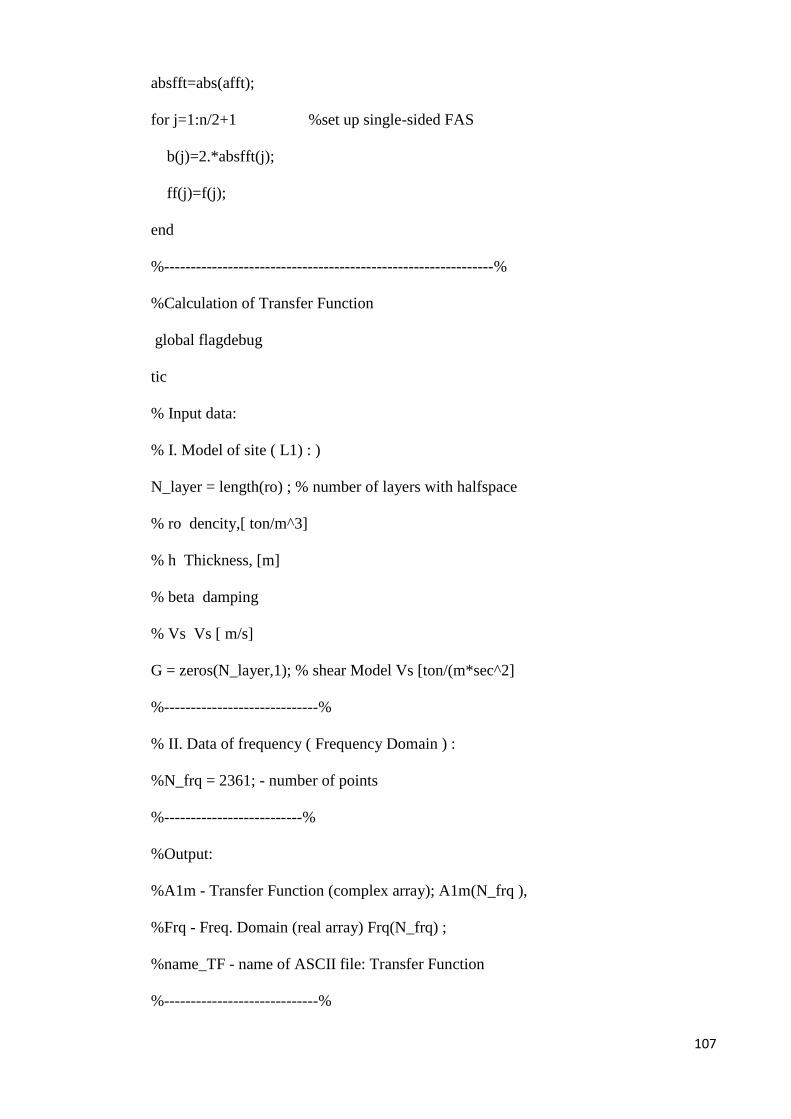
107

absfft=abs(afft);

for j=1:n/2+1 %set up single-sided FAS

b(j)=2.*absfft(j);

ff(j)=f(j);

end

%--------------------------------------------------------------%

%Calculation of Transfer Function

global flagdebug

tic

% Input data:

% I. Model of site ( L1) : )

N_layer = length(ro) ; % number of layers with halfspace

% ro dencity,[ ton/m^3]

% h Thickness, [m]

% beta damping

% Vs Vs [ m/s]

G = zeros(N_layer,1); % shear Model Vs [ton/(m*sec^2]

%-----------------------------%

% II. Data of frequency ( Frequency Domain ) :

%N_frq = 2361; - number of points

%--------------------------%

%Output:

%A1m - Transfer Function (complex array); A1m(N_frq ),

%Frq - Freq. Domain (real array) Frq(N_frq) ;

%name_TF - name of ASCII file: Transfer Function

%-----------------------------%

108

Vs_sum = 0;

h_sum = 0;

ro_sum = 0;

for j = 1:(N_layer -1),

Vs_sum = Vs_sum + h(j)*Vs(j);

h_sum = h_sum + h(j);

ro_sum = ro_sum + h(j)*ro(j);

end;

%h_sum

Vs_mean = Vs_sum/h_sum;

ro_mean = ro_sum/h_sum;

F_mean = Vs_mean/(4*h_sum);

A_mean = (Vs(N_layer)*ro(N_layer)) / (Vs_mean*ro_mean);

for j = 1: N_layer,

G(j) = ro(j)*Vs(j)^2;

tmp_str(j).t = [ ' : ' num2str(j) ' : ' num2str(ro(j)) ' : ' num2str(h(j)) ' : ' num2str(beta(j)) ' :

' num2str(Vs(j)) ' : ' num2str(G(j ))];

end;

%------------------------------%

if flagdebug,

h_sum;

Vs_mean;

ro_mean;

F_mean;

A_mean;

%------------------%

109

disp ( ' Input Model') ;

disp ;(' ---------------------------------------------------------------------');

disp( [ ' : # : ro : h : beta : Vs : G;)'])

disp( [ ' : # : [t/m^3] : [m] : : [m/s] : [ ton/(m *sec^2'] ) ;

disp ;(' -----------------------------------------------------------------------------');

for j = 1: N_layer,

disp( tmp_str(j).t);

end;

disp ;(' --------------------------------------------------------------------------------')

%==============================================%

% Data for Legend:

lin = ' ---------------------------------------------------------' ;

lgnd(1).t = ' Input Model;';

lgnd(2).t = lin ;

lgnd(3).t = ' : # : ro : h : beta : Vs : G; ';

lgnd(4).t = ' : # : [t/m^3] : [m] : : [m/s] : [ ton/(m *sec^2)]' ;

lgnd(5).t = lin ;

for j = 1: N_layer,

lgnd(5 + j).t = tmp_str(j).t;

end ;

lgnd(6 + N_layer).t = lin;

%=================================%

end;

% if flagdebug,

%Frequency Domain:

N_frq=n+1;

110

Frq = [0:(N_frq-1)]'*ff(j);

%=====================================================%

%Computation Transfer Function :

%Initialization values and define arrays:

K = zeros(N_frq, N_layer);

E = zeros(N_frq, N_layer); % Amplitudes UP

F = zeros(N_frq, N_layer); % Amplitudes DOWN

A1m = zeros(N_frq , 1); % Transfer function : between layers : 1 & m

A1m_cmplx = zeros(N_frq , 1); % Transfer function : between layers : 1 & m

G_astr = zeros(1 , N_layer );

ALFA = zeros(1 , (N_layer -1));

gamma = zeros(1 , (N_layer -1 ));

E(:,1) = 0.5 ; % Amplitudes UP

F(:,1) = 0.5 ; % Amplitudes DOWN

%-------------------------%

%Computation values, independent from frequency:

for j = 1:(N_layer ) , % Prepare Loop : on Layers of Model

% disp( [ '# ' num2str(j ;) ] )

Gastr0 = G(j)*( 1 + beta(j)*2*i ) ; % formula #7 : Upgraded : 25.04.2004

G_astr(j) = Gastr0;

end; % for j = 1 : (N_layer -1) , % Prepare Loop : on Layers of Model

%------------------------------------------%

for j = 1:(N_layer - 1) , % Prepare Loop : on Layers of Model

% disp( [ '# ' num2str(j) ] )

alfa0 = sqrt( ro(j)* G_astr(j) / ( ro(j + 1)* G_astr(j + 1) ) ) ; % formula 19

%-------------------%

111

ALFA(j) = alfa0;

gamma(j) = sqrt( ro(j)/ G_astr(j ));

end; % for j = 1 : (N_layer -1) , % Prepare Loop : on Layers of Model

%------------------------------------------%

%Main Loops:

for k = 1:N_frq , % External Loop ( #1 ) : on Frequency

omega = 2*pi*Frq(k); % round frequency

for j = 1 : (N_layer -1) , % Internal Loop ( #2) : on Layers of Model

%-------------------%

% K(k,j) = omega * sqrt( ro(j)/ G_astr(j) ); % formula # 6

K(k,j) = omega * gamma(j); % formula # 6

%-------------------%

exp1 = exp( i*K(k,j)*h(j));

exp1d1 = 1/exp1;

%------------------------------%

E(k,j + 1) = 0.5* E(k,j)*( 1 + ALFA(j) )*exp1 + ...

5.0*F(k,j)*( 1 - ALFA(j) )*exp1d1 ; % formula 17

%-------------------%

F(k,j + 1) = 0.5* E(k,j)*( 1 - ALFA(j) )*exp1 + 5.0 *F(k,j)*( 1 + ALFA(j) )*exp1d1; %

formula 18

end; % Loop #2 : j

%-------------------%

A1m_cmplx(k) = (0.5 / E(k ,N_layer)); % + F(k ,N_layer)/F(k,1) ) ; % % % formula 22

A1m(k) = abs( A1m_cmplx(k)); % + F(k ,N_layer)/F(k,1) ) ; % formula 22

end; % Lopp #1 : k

%-----------------------------%

112

if flagdebug,

%Drawing Transfer Function :

%-----------------------------%

plot( Frq(:) , A1m(:) , 'linewidth' , 1.5 , 'color' , 'k' ) ;

xlabel( 'Frequency [Hz]' , 'fontsize' , 12 ) ;

ylabel( 'Amplitude' , 'fontsize' , 12 ) ;

title(' Transfer Functon by Shake : for input model ' , 'fontsize' ,12 ) ;

lgnd1 = { lgnd(1:(N_layer+6)).t } ;

legend( lgnd1 ) ;

grid on;

end; % if flagdebug,

%--------------------------------%

%calculation of output motion

for k=1:n+1

accs(k)=afft(j)*A1m(k); %compute output motion in frequency

end

for k=1:n/2+1

accs_t(k)=2.*abs(accs(k)); %compute FAS of output motion

end

%% Design High Pass Filter

fs = 8000; % Sampling Rate

fc = 0.6/1; % Cut off Frequency

order = 6; % 6th Order Filter

%% Filter Surface Acceleration Signals

[b1 a1] = butter(order,fc,'high');

af=filtfilt(b1,a1,acc);

113

atime=n*real(ifft(af));

% subplot(5,1,5)

%plot(t,atime)

subplot(5,1,1)

plot(t,accr);

ylabel('BedrockMotion')

subplot(5,1,2)

plot(ff,b);

subplot(5,1,3)

plot( Frq(:) , A1m(:) , 'linewidth' , 1.5 , 'color' , 'k' ) ;

ylabel('Amplitude')

subplot(5,1,4)

plot(ff,accs_t);

subplot(5,1,5)

plot(t,atime);

ylabel('SurfaceMotion')

Code1_test2.m

%Conversion of the bedrock motion to displacement

%% accelerations are integrated twice to produce displacements

load data.dat ;

n;

dt;

t;

accr;


114




%% Filter Acceleration Signals


accrf=filtfilt(b1,a1,accr);

%% First Integration (Acceleration - Veloicty)

velocity=cumtrapz(t,accrf);

%% Filter Veloicty Signals


velf = filtfilt(b2,a2,velocity);

%% Second Integration (Velocity - Displacement)

Displacement=cumtrapz(t, velf);

%---------------------------------------------------------%

%plot figures

%figure 1

subplot(3,1,1);

plot(t,accrf,'r'); hold on

plot(t,accr)

xlabel('Time (sec)')

ylabel('Acceleration (mm/sec^2)')

%figure 2

subplot(3,1,2);

plot(t,velocity)


ylabel('Velocity (mm/sec)')

115

%figure 3

subplot(3,1,3);

plot(t,Displacement)


ylabel('Displacement (mm)')

Code1_test3.m

%Based on,

% T(z) = 0.5*rho*z*(surface acceleration+acceleration at depth z)

% Zeghal & Elgamel quote this.

%

%function [T] = calculatestress(z,a,density)

%---------------------------------------------------

%Input data

%data.dat

%n

%accr

%h Thickness of layer

%ro_k

%---------------------------------------------------

%Input data

load data.dat;

n;

accr;

accr=reshape(accr,787,[]);

h;

ro_k;

116

density=ro_k*0.10197;

atime;

T = 0.5*density(2)*h(2)*(atime(:,2) + accr(:,2));

T(1:200)=0.0;

T(487:787)=0.0;







afT=filtfilt(b1,a1,T);

peakstresses = [max(T); min(T)];

figure(11)

subplot(2,1,1)

plot(afT/1000, 'color', 'R'); ylabel('Shear stress (kPa)'); xlabel('Time (sec)');

Code1_test4.m

%function [g] = calculatestrain(z, u)

%Input data

%Displacement;

%h

%-------------------------------------------------------

%Input data

Displacement;

m=length(Displacement);

117

dt=0.02; %time step

t=0.0:dt:m*dt; %set up time vector

u=Displacement;

u=reshape(u,787,[]);

h;

dh = [h(7) - h(1), h(19) - h(7), h(19) - h(1)];

g = (((u(:,3) - u(:,2))*dh(1)/dh(2)) + ((u(:,2) - u(:,1))*dh(2)/dh(1)))/dh(3);







afg=filtfilt(b1,a1,g);

peakstrains = [max(g); min(g)];

figure(11)

subplot(2,1,2)

plot(afg*100,'r'); ylabel('Shear strain (%)'); xlabel('Time (sec)');

Code1_test5.m

%Calculating the Damping ratio 'e'.

%Inpput data

T; %Shear stress

g; %Shear strain

G; %Max Moduli

%---------------------------

118

G=reshape(G,1,[]);

%----------------------------

%Calculate Moduli

for n=1:787

moduli(n)=T(n,1)/g(n,1);

end

%---------------------------

%Input PI for soil based on the type of the soil(%)

PI=0; %nonplastic soil

PI=30; %plastic soil

%---------------------------

%Calculate Damping Ratio

for m=1:12

e(m)=0.333*((1+exp(-0.0145*(PI^1.3)))/2)*((0.586*(moduli(1,m)/G(1,m))^2)-

1.547*(moduli(1,m)/G(1,m))+1);

end

Code1_test6.m

%Hysteretic loop

%Input data

G; %Max moduli

g; %shear strain

T; %shear stres

T_Max=max(T);

T_min=min(T);

g_Max=max(g);

119

g_min=min(g);

%--------------------------

%backbone function for hysteresis loop backbone

for k=1:12

F_bbM(k)=(G(1,k)*g(k,1))/1+(G(1,k)/T_Max)*abs(g(k,1)); %backbone function

F_bbm(k)=(G(1,k)*g(k,1))/1+(G(1,k)/T_min)*abs(g(k,1));

end

plot(F_bbM*100,F_bbm*100) %plot backbone function

ylabel('Shear stress'); xlabel('Shear Strain (%)');

Code1_test7.m

%Response Spectrum Analysis

%Input data

dt=0.02;

load elcentro.dat

Ag=elcentro(:,2);

zet=2;

g=9810;

endp=5;

%---------------------------%

u=zeros(length(Ag),1);

v=zeros(length(Ag),1);

ac=zeros(length(Ag),1);

Ag(end+1)=0;

T(1,1)=0.00;

fs(1,1)=0.00;

120

for j=1:round(endp/dt) % equation of motion(Newmark linear method)

omega(j,1)=2*pi/T(j); % Natural Frequency

m=19.6602929705203;

k=(omega(j))^2*m;

c=2*m*omega(j)*zet/100;

K=k+2*c/dt+4*m/(dt)^2;

a=4*m/dt+2*c;

b=2*m;

for i=1:length(u)-1

u(1,1)=0; %initial conditions

v(1,1)=0;

ac(1,1)=0;

df=-(Ag(i+1)-Ag(i))+a*v(i,1)+b*ac(i,1); % delta Force

du=df/K;

dv=2*du/dt-2*v(i,1);

fs(i+1,1)=fs(i,1)+K*du;

u(i+1,1)=u(i,1)+du;

v(i+1,1)=v(i,1)+dv;

ac(i+1,1)=(Ag(i+1)-c*v(i+1)-fs(i+1))/m;

end

Sd(j,1)=max(abs((u(:,1))));

%Sv(j,1)=max(abs(v));

%Sa(j,1)=max(abs(ac))/g;

Spv(j,1)=Sd(j)*omega(j);

Spa(j,1)=Sd(j)*(omega(j))^2/g;

T(j+1,1)=T(j)+dt;

121

end

Ag(end)=[];

T(end)=[];

Sd(2,1)=0; Spv(1:2,1)=0;Spa(1:2,1)=max(abs(Ag))/g;

figure('Name','Spectral Displacement','NumberTitle','off')

plot(T,Sd,'LineWidth',2.)

grid on

xlabel('Period (sec)','FontSize',13);

ylabel('Sd (mm)','FontSize',13);

title('Displacement Spectrum','FontSize',13)

figure('Name','Spectral velocity','NumberTitle','off')

plot(T,Spv,'LineWidth',2.)

grid on


ylabel('Spv (mm/s)','FontSize',13);

title('Pseudo Velocity Spectrum','FontSize',13)

figure('Name','Pseudo Acceleration Spectrum','NumberTitle','off')

plot(T,Spa,'LineWidth',2.)

grid on


ylabel('Spa (g)','FontSize',13);

title('Pseudo Acceleration Spectrum','FontSize',13)

122

APPENDIX B

Program Interface

A prototype of the numerical methods used in this research are prepared and written in

MATLAB (Refer to Appendix A). The syntax of a MATLAB program is similar to

other languages such as FORTRAN and BASIC, however, it contains more high level

functions that allow many complicated calculations and graphics command to be

proceed easily. These MATLAB codes are finally converted to C# for the actual site

response analysis program.

Program Display

The interface of the program consists of the several elements; Title Bar, Menu Bar and

Main Tabs (Figure 1).

Figure B.1: New program code interface.

123

Title Bar:

The Title Bar at the top left corner of the program windows shows the name of the

program and the current name of the project.

Menu Bar:

The Menu Bar located directly below the Title Bar, including all the pull-down menus.

Each of the menu options consists of a list of commands that can be selected according

to the computation procedure. The Menu Bar designed with the logical order of the

operations and hindered access to further operations until all the necessary data have

been added. There is also a help button to instruct the user how to operate the system.

Main Tabs:

The main tabs that are located below the Title Bar indicate the step by step procedure of

the program. Each tab have separate interface with different preferences for input data,

manual options that the user needs to choose manually depends on the requirements,

and other features such as graphs and results.

Menus and Tabs

The description of menus are as follows;

1. File Menu

The file menu contains several commands. The user can choose a new project or open

the existing ones, and then save the project as a new project or the existing one. The

pull-down menu “File” is shown in Figure 2.

124

Figure B.2: The pull-down menu “File”.

2. Data Menu

The Data menu is consisting of 2 options where the user can import soil input data or

the earthquake data. Figure 3 shows the pull-down “Data”.

125

Figure B.3: The pull-down menu “Data”.

3. Help Menu

The Help menu is an option for the user to learn about the program, lean about how

does it work and look up necessary instructions for the program to run. The pull-down

menu “Help” is shown in Figure 4.

126

Figure B.4: The pull-down menu “Help”.

The Tabs are presented as follows;

1. Project

o Project Details

o Soil Materials

2. Soil Profile

3. Earthquake

4. Results

Project:

This section is divided into two tabs; Project Details, where the user is able to insert the

project name and the project details if needed in the spaces defined in the tab, and the

Soil Materials where user is able to choose an appropriate curve for the soil type. There

is an option where the user can choose either “sand” or “clay” as a type of a soil

regarding to the soil profile of the project in hand, to identify the G/Gmax vs. shear

strain values and Damping ratio in order to compare it to the calculated damping ratio

done by the new program code (Figure 5).

127

Figure B.5: Project tab.

Soil Profile:

This tab has two sections. One is the table for input data, the other one is the graphs

presented at the bottom of this tab. In the table columns such as; Soil material type,

Thickness of layer, Total unite weight and the shear wave velocity are to be filled by

user, while the rest of the columns will be calculated by the new program code. Figure 6

shows a sample ran by new program code.

128

Figure B.6: Soil profile tab.

Earthquake:

This tab is for the user to insert the earthquake data of the project in hand. The time

period also should be identified by the user (Figure 7).

Figure B.7: Earthquake tab.

129

Results:

This tab contains of several tabs presenting all the results computed such as; Shear

Stress, Shear Strain, Amplification ratio, Fourier Amplification, Acceleration,

Hysteresis loop and finally Response Spectrum (Figure 8).

Figure B.8: Result tab.

Documents

EARTHQUAKE SITE RESPONSE ANALYSES FOR SOIL NASIM …studentsrepo.um.edu.my/9234/8/Nasim_Sarrafi_Aghdam-Thesis_201… · Tajuk Kertas Prokjek/Laporan Penyelidikan/ Disertasi/Tesis