Early Voting Laws, Voter Turnout, and Partisan Vote

Composition: Evidence from Ohio∗

Ethan Kaplan† Haishan Yuan‡

March 28, 2018

Abstract

We estimate effects of early voting on voter turnout using a 2010 homogenization law

from Ohio which forced some counties to expand and others to contract early voting.

Using voter registration data, we compare individuals who live within the same 1 square

mile block but in different counties. We find substantial positive impacts of early voting

on turnout equal to 0.24 percentage points of additional turnout per additional early

voting day. We also find greater impacts on women, Democrats, Independents and

those of child-bearing and working age. We simulate impacts of national early day

laws on recent election outcomes.

1 Introduction

Since its birth, the right to vote has been highly contested. Originally, in most states, the

voting franchise was restricted to propertied white adult men. Even before the Civil War,

political battles were fought to expand the franchise to include those without property. After

the civil war, in 1870, the Fifteenth Amendment granted African-Americans the right to vote.

∗We thank Jeffrey Ferris for numerous extremely valuable conversations. We thank comments madeby Michael Hanmer, Jared McDonald, and seminar participants at Australian National University, CapitalUniversity of Economics and Business in Beijing, Georgetown University, the London School of Economics,the Paris School of Economics, the University of Maryland at College Park, the University of Melbourne, andWarwick University. We thank Jacqueline Smith for suggesting the idea behind Section 6 of the paper. Wethank Lucas Goodman, Max Gross, Ann Hoover, Yuting Huang, Alejandro Perez-Suarez, and Cody Tuttlefor excellent research assistance. All mistakes are, of course, our own.†University of Maryland at College Park; e-mail: kaplan@econ.umd.edu; address: 3114 Tydings Hall,

Department of Economics, University of Maryland, College Park, MD 20742, U.S.A.; Tel.: +1 301 405 3501‡University of Queensland; e-mail: h.yuan@uq.edu.au; address: Level 6, Colin Clark Building (39), School

of Economics, University of Queensland, St Lucia QLD, Australia 4072; Tel.: +61 7 3365 4027

1

However, through a battery of state laws passed starting in the late 1870s, poll taxes and

literacy restrictions were placed upon voting in most Southern states which effectively limited

minority participation in voting. Women were enfranchised at the state level starting with

Wyoming in 1869. States increasingly passed female suffrage laws until the 19th Amendment

to the Constitution was passed in August of 1920. State-level estrictions upon voting, which

dramatically reduced African-American participation in voting, remained in place until the

1965 passage of the Voting Rights Act under the Johnson Administration.

In recent years, political parties have been very active in passing legislation at the state

level expanding or limiting ease of access to voting. State level legislative activity regulating

voting has been primarily concentrated in 4 areas: (1.) Legal changes affecting the ease

of voter registration, (2.) Laws expanding or contracting the ability of felons to vote, (3.)

Laws which tighten or loosen identification requirements at the ballot box, and (4.) Laws

expanding or contracting the prevalence of early voting availability.1

Early voting in particular and pre-election voting in general have become common forms

of voting. Though pre-election voting began first in California back in 1976 and then in

Texas in 1987, most of the rollout of early voting happened in the 1990s and 2000s (Biggers

and Hanmer, 2015).2 As of 1992, 7% of individuals cast their ballots using some form of pre-

election voting (McDonald, 2016). By 2008, the beginning of our main sample, pre-election

voting had expanded to over 30% of ballots cast nationally; these numbers rose to 34.5%

by 2016. Initially, pre-election voting was primarily in the form of mail balloting. However,

in recent years, the importance of in-person early voting has risen. In 2016, over 47 million

of the approximately 136.5 million ballots cast used some form of pre-election voting. 23

million of these were cast in-person. Early voting is potentially important in the United

States because election day is not a national holiday nor a weekend day in the United States

as it is in many developed countries.

In the 2016 general election, there were substantial differences across states in early

voting availability. On the one hand, ten states had no in-person early voting.3 At the other

extreme, Minnesota provided 46 days of early voting. The changes in early voting which

have occurred in the past two decades, have predominantly occurred at the state and county

levels. Reductions in early voting have accelerated since the Supreme Court struck down the

formulas used in Section 4 of the Voting Rights Act. Within months of the Supreme Court’s

1Early voting is otherwise known as “no-excuse” absentee voting.2In this paper, we will refer to in-person early voting as early voting. The other form of early voting is

absentee balloting. Where we discuss the sum of in-person early voting plus absentee balloting, we will referto it as “pre-election voting”.

3The ten states without in-person early voting were Alabama, Connecticut, Delaware, Michigan, Missis-sippi, New Hampshire, Oregon, Pennsylvania, Rhodes Island, and Washington

2

Shelby County vs. Holder (2013) decision, restrictive voting laws had been introduced in

state legislatures in Alabama, Arizona, North Carolina, Ohio, South Carolina, Texas, and

Wisconsin.

Of course, it is not clear that expanding opportunities to vote will actually increase

voting. Some political scientists who have studied early voting have estimated positive

effects on turnout (Herron and Smith, 2012; Herron and Smith, 2014), others have found no

systematic overall impact upon turnout (Gronke et al., 2007) and others yet have found that

early voting expansion has reduced turnout (Burden et al., 2014). The idea that early voting

may reduce turnout may sound strange at first. However, there is a well documented effect

that people vote in part to tell others (DellaVigna et al., 2017). It is also possible that voters

turn out in order to be seen voting and that early voting, by spreading voting across many

weeks, reduces the link between being seen and voting. Burden et al. (2014) have a similar

explanation for their seemingly perverse findings. They claim that early voting weakens a

sense of common solidarity which is important for motivating high turnout.

Unfortunately, given the importance of the subject, there are surprisingly few studies

on the impacts of differences in state voting laws in general and early voting in particular.

Moreover, what studies exist suffer from plausible endogeneity bias. Gronke et al. (2008) has

an early review of the academic literature on the effect of convenience voting (early voting,

absentee balloting, electronic voting, and voting by mail). The early literature largely relied

time series variation (Gronke et al., 2007) within a state. This does a decent job of controlling

for endogeneity arising from characteristics of the electorate but does not control well at all

for endogeneity due to characteristics of the election.

Burden et al. (2014) and Herron and Smith (2014) are more recent papers which esti-

mate impacts of early voting and use different sources of variation. They also focus upon

the impact of early voting laws rather than photo ID laws and are thus more similar to our

own paper. Burden et al. (2014) estimates the impact of of early voting laws on individ-

ual turnout using cross-state variation in legal changes which expanded or contracted the

availability of early voting. They run regressions with county level turnout data as well as

individual regressions with data from the CPS voter supplement. The identification comes

from assuming that state-level trends are uncorrelated with other determinants of turnout

conditional upon controls.

Herron and Smith (2014) also examine the impact of early voting using variation solely

within Florida when Florida reduced early voting from 14 to 8 days. They use voter reg-

istration data and thus view not only whether people vote but also when they vote. They

also view race at the individual level. They find a decline in voting and particularly in early

voting. They also find that the effects are concentrated in minority groups and registered

3

Democrats. However, their identification comes from pure time series variation and thus it is

hard to separate the effect of the legal changes to early voting from secular trends in voting

patterns or election specific effects which may have differentially impacted African-Americans

and Democrats and particularly so during the Obama years.

Card and Moretti (2007) estimated the impact upon turnout of new and improved voting

technology using the roll out of the Help America Vote Act. They use cross-county variation

controlling for covariates. This variation is cleaner than much of the other literature in that

most races that voters pay attention to are at the state level (presidential races at the state

level, Senate elections, and Governor races). Using cross-county variation and controlling

for state fixed effects, Card and Moretti (2007) substantially reduce electoral endogeneity.

However, they do not effectively control for endogeneity due to voter demographics. Voters

of different age, race, sex and partisan leanings have different propensities to turn out and

these are often election-specific.

In this paper, we estimate the impact of early voting on voter turnout. We do this using

voter registration data from Ohio and look at turnout before versus after Ohio homogenized

early voting availability across counties. In many states, counties differ in the number of

hours and days that they are open. In this paper we make use of a natural experiment in

Ohio which homogenized the days and even exact hours of early voting across counties in

Ohio. This change was passed by Republican Governor John Kasich in time for the general

election in 2012.

Our paper, rather than trying to add in covariates to control for unobservables, tries to

construct treatment and control groups which are similar. We do this using geographical

discontinuities in treatment across county borders. We thus follow the literature using spa-

tial neighbors with differential spatial treatment (Dube et al., 2010; Snyder and Stromberg,

2010; Spenkuch and Toniatti, 2016). We also add to a growing literature within economics

estimating the impact of electoral interventions using more credible research designs (Bra-

connier et al., 2016; Naidu, 2012; Pons, forthcoming). Since we use individual level data from

the Ohio voter registration database, we have tight standard errors. However, our spatial

discontinuity approach also allows for credible identification.

We also show estimates using cross county variation. However, we only use within-state

variation which means that we control for state level candidate quality such as US Senator

and Governor quality as well as competitiveness in Senate, gubernatorial and presidential

elections. We also show that cross-county variation in our Ohio sample is not as clean as

our geographical discontinuity estimates. As we increase our bandwidth, our estimates fail

demographic and political placebo tests for endogeneity.

Our best specification estimates effects within 1 × 1 mile blocks which straddle county

4

lines where counties differentially changed early voting availability due to the change in state

law. Besides looking at aggregate turnout effects, we estimate differential turnout effects for

weekend days, same day registration days, and days where polls were open until 7 PM or

later. We also estimate models where we allow for non-linearities in treatment. We not only

show estimates by different types of treatment but also by different types of voters. We

estimate the impacts differentially by sex, party, and age. Overall, we find that an extra day

of early voting increases turnout by 0.24%.

Finally, we use our estimates of partisan effects to linearly simulate the impact of hypo-

thetical national early voting election laws. We find limited impacts on outcomes in the 2012

election. However, for the 2016 election, we find that eliminating early voting would have

reduce Democratic House seats by 10 whereas mandating 23 days nationally (the current

level in Ohio) would have tilted the presidential election to Hillary Clinton. We find that

mandating 46 days nationally (the current level in Minnesota) would also have shifted three

Senate seats and the balance of the Senate to the Democrats.

In Section 2, we give an overview of the electoral law change we use in the state of Ohio.

In Section 3, we describe our data. In Section 4, we present our methodology. In Section

5, we discuss our main estimates. In Section 6, we show results of simulations of national

electoral law changes on election outcomes. Finally, in Section 7, we conclude.

2 Ohio Election Law Changes

Like many states, Ohio saw large expansions of early voting in the 2000s. In 2002, 6.8%

of voters cast pre-election ballots. In 2005, Ohio passed legislation allowing for in-person

early voting. By 2008, 29.7% of the electorate voted pre-election (Kaltenthaler, 2010). In

the general election of 2012, the percent making use of in-person voting before the election

was 10.6% and by 2016, it had risen to 11.8%.4 The contraction in early voting availability

in urban areas happened during a period of increased popularity of early voting.

The expansion in early voting was differential across counties. Urban, Democratic areas

expanded early voting at a faster rate than rural, Republican ones. By 2008, rural Pickaway

County was open for 109 hours of early voting, spanning a total of 11 days including only 1

weekend day, 2 days of same day registration and no weekend days of same day registration

or Sunday voting days. By contrast, urban Franklin County, which contains the city of

Columbus, was open for a total of 340 hours spread over 35 days including 7 days of same

4These numbers on the prevalence of in-person early voting were obtained from the Ohio Secretary ofState website: https://www.sos.state.oh.us/SOS/elections/Research/electResultsMain.aspx.

5

day registration voting5, 10 weekend days of early voting including 2 same day registration

weekend voting days, and 5 Sundays.

In November, 2010, Republican John Kasich defeated incumbent Democrat Ted Strick-

land for the Governorship. In addition, the State Senate remained majority Republican

and the State House of Representatives switched majority control to the Republican party.

Under unified Republican control, the government passed State Bill 295 which homogenized

early voting across counties. Each county early voting station was required to be open the

exact same hours on the exact same days as all other counties. This meant that Cuyahoga

County with a population of 1.266 million in 2012 ended up with identical hours of early

voting as rural Pickaway County with population 56,000. The law eliminated early voting

for the three days prior to the election. This meant that early voting in the weekend before

the election was eliminated from all counties. The total number of days was changed to 26

with 4 same-day registration days though no weekend days of same day registration and 2

Saturdays though no Sundays.

Large pre-2012 discrepancy across counties within Ohio led to large differential changes

due to the state policy changes implemented in 2012. On the one hand, Cuyahoga, Franklin

and Summit Counties all saw reductions of 9 days of early voting. This reduction was largely

due to reduced weekend voting. In each case, 8 of the 9 days were Saturdays or Sundays.

Moreover, Cuyahoga’s total hours were reduced by 56.5; Franklin’s and Summit’s each by

94 hours. By contrast, Wyandot and Pickaway both increased their weekend early voting

by one day. Though Wyandot’s total number of days of early voting availability did not

increase, Pickaway’s did by 15 days. Wyandot’s total hours of early voting increased by 100

and Pickaway’s by 137.

The contracting counties were quite different from the expanding ones in terms of political

orientation. Cuyahoga, which contains Cleveland, is a large urban area with a 1.28 million

population as of the 2010 census. It is 30.3% African American and had a 68.8% vote share for

Obama in 2008. Franklin County, containing Columbus, Ohio, is 21.2% African-American,

has a population of 1.16 million and had a 60.1% Obama vote share in 2008. Summit County,

containing Akron, Ohio, has a population of 540,000, is 13.2% African-American and had a

56.7% Obama vote share in 2008. By contrast, Pickaway, which is a rural county without

a major city, has a population of less than 60,000, is 3.7% African-American and had an

5All states except North Dakota require registration in order to vote. Ten states and Washington, D.C.allow registration on election day. All other states require pre-registration. In Ohio, registration must occur30 days or more before the election in order to participate in a national general election. In practice thishas meant 28 days before the election because 30 days before the election was a Sunday and the next dayhas been Columbus day. The State of Ohio always extends the deadline to the next business day if it fallson a weekend or a holiday. In years where early voting extended before the deadline, citizens could registerto vote and vote at the same time in an early voting station. This is called same day registration.

6

Obama vote share of 39.8%; similarly, Wyandot, another rural county, has a population

slightly above 20,000, is 0.4% African-American and had a 38.6% Obama vote share.

Of course, comparing the counties which contracted versus expanded early voting risks

strong endogeneity bias due to correlation of differences in demographics and thus voting

trends with the magnitudes and signs of early voting changes. Our main strategies thus rely

on finding locations with differential contractions and expansions but similar demographics

and thus voting trends.

In Figure 1, we show the changes in early voting days between 2008 and 2012 by county.

We see large reductions in early voting days in 2012 relative to 2008 for the large urban

counties of Cuyahoga which contains Cleveland, Summit which contains Akron and Franklin

which contains Columbus. We also show changes of early voting by six other different mea-

sures across counties between 2008 and 2012 in Figure A.1. These measures of early voting

access are the numbers of weekend days, days allowing same day registration, days open

late, weekdays, Saturdays, and Sundays. For most measures, urban counties experienced

large reductions of early voting in 2012, while rural counties saw increases, no changes, or

relatively small decreases.

3 Data

Our main data source is the voter registration database from the State of Ohio. The

database contains full name, exact date of birth, date of registration, individual voting

history dating back to the year 2000, address of residence including county, precinct, and

party for those who have participated in primaries.6

Ohio is an open primary state. Therefore, the data does not contain party registration but

instead records the party of the primaries the voter participated in. We record an individual

as a Republican if the most recent primary they participated in was a Republican party

primary, a Democrat if the most recent primary they participated in was a Democratic

party primary, and an Independent for those who have never participated in a primary.

43.1% of registered individuals are listed as Independent in our sample, 30.4% are listed as

Democrats and 26.5% as Republicans.7

Using ArcGIS and Google Maps, we geocoded each individual registration address into

6The registration data for Morgan County is missing from the files that we obtained from the Secretaryof State of Ohio. Morgan County is one of the smallest population counties in Ohio. It has a total of 14,904residents out of state with 7.6 million registered voters. Thus, less than 0.1% of Ohio voters who reside inMorgan County are not included in our sample.

7In our data, which goes back to the year 2000 and covers eight national primaries, only 7.2% of registeredvoters voted in a Republican primary for one election and a Democratic primary for another election.

7

longitude and latitude. We then divide the State of Ohio into a mutually exclusive and

exhaustive set of equal-sized square geographical blocks.

We additionally use the geocoded locations to assign each individual to a census block

group and we then merge demographic information on race, education, and income at the

census block level to each individual. Thus each individual within a census block-group has

a set of demographic variables which do not vary across individuals within the same census

block-group. These set of variables include % white, % black, % Hispanic, median household

income, % high school dropouts, and % college graduates. In approximately 10 percent of

cases, ArcGIS does not match to a census block group. In these cases, we compute minimum

distance to each census block group in the state using latitude and longitude and assign an

individual to the geographic centroid of the closest block group.8 For consistency, we match

all individuals to census block groups using the minimum distance to block group centroids.9

Next, for each of Ohio’s 88 counties, we obtain from each individual county secretary of

state the exact hours of early voting availability for each day of early voting. We do this for

the years 2008 and 2012. We use this data to compute our main treatment variable: number

of days of early voting by county for each election. We also compute other treatment variables

which we use for estimating heterogeneity in the treatment effect by type of treatment. These

additional variables are number of hours, number of weekend days, number of Saturdays,

number of Sundays, number of week days, number of days of same day registration, and

number of days where polls were open until 7 PM or later.

We also compute for each individual, the probability that their sex is female. Ohio voter

registration data does not record sex. However, the social security administration keeps a

registry of all baby first names by sex. These lists are maintained by year. For confidentiality

reasons, the data are truncated. Names with fewer than 5 occurrences in a given year for a

given sex are not reported. As an example, in the year 1980, 94.8% of births in the United

States are in our national baby name list. We obtained both the national lists as well as

the lists for the State of Ohio. For each year and for each of the two lists (national and

Ohio), we compute the probability that a name is female as the proportion of babies with

that name who are female. If a name is not listed for a particular gender, we assume that

zero babies were born with that name for that gender. We use the probability that a baby

is female as our sex variable. We drop unmatched observations. 95.6% of individuals in our

voter registration file match to one of the first names in the national baby name file in their

birth year; 89.9% match to one of the first names in the Ohio state baby name file in their

8We have run our results dropping the individuals with imputed census block group and the results arenear identical.

9Estimates change little when we use a sample by matching through either ArcGIS or minimum distance,or by dropping the individuals unmatched to a census block group by ArcGIS.

8

birth year.

Finally, we use the self-reported ideology question and the party affiliation question from

the 2016 Cooperative Congressional Election Study (CCES). The CCES is a stratified sample

survey, administered by YouGov, which links questionnaire answers by respondents to actual

voting records. We use 40,784 observations from the CCES to show ideological differences

by party affiliation.

4 Methodology

We employ four empirical strategies to estimate the impact of restrictive voting laws

upon voter turnout. The last of these is our preferred strategy. The first is the standard

county-level difference in differences estimator where we regress voter turnout on treatment

controlling for a county fixed effect and a time fixed effect. Our main treatment variable

is the number of days of early voting. However, we also estimate models where we are

interested in the heterogeneity of the treatment effect across different types of treatment (i.e.

weekdays versus weekends, same day registration days versus normal days, days when early

voting extends to 7 PM or later versus regular hour days). In these cases, we simultaneously

regress upon multiple regressors. In order to compare our difference-in-differences estimates

to estimates of the impacts of voting interventions at the county level, ours differ only in

that we do not use cross state variation. Our estimation equation is given by:

Vict = αt + φc + T′

ctβ + εct + θict (1)

where Vic is a binary variable equal to 100 if voter i turns out in county c for the general

election in time period t and is zero otherwise, αt is an election-year fixed effect, φc a

county level fixed effects, Tct is a vector of treatment variables, εct is a mean zero serially

correlated county-specific random term which is independent across counties, and θict is an

idiosyncratic individual level random term. We choose our dependent variable to take on

the values of 100 or zero so that our estimates are expressed in units of percentage point

effects per unit of treatment. We cluster standard errors for equation (1) at the county level.

This specification assumes that aggregate voting trends by county are uncorrelated with

treatment. In particular, it assumes that trends in voter turnout in urban counties which

saw large reductions in early voting would have been the same as in rural counties whose

early voting access stayed constant or increased absent the early voting changes.

Our second main specification replaces the county-level fixed effects φc from equation (1)

with individual fixed effects γi. Since there are no covariates in these regressions, the switch

9

to individual fixed effects operates by dropping those who were not registered continuously

over the time period. First time registrants include those who were previously too young

to register, those who were not too young but had never registered or voted, and those

who moved to Ohio from out of state.10 The individual fixed effects identification strategy

relies upon weaker assumptions than the identification strategy assumed by the best related

papers in the observational methods literature such as Card and Moretti (2007) which use

county instead of individual fixed effects because the county fixed effects results are not

robust to demographic shifts in the registered electorate. Our individual fixed effects model,

by contrast, correctly estimates treatment effects for those whose registration did not change

across elections. However, this is still under the maintained assumption that voting trends

for registered individuals across counties was uncorrelated with treatment. Our model of

turnout, in this case, is given by:

Vict = αt + γi + T′

ctβ + εct + θict (2)

We next restrict our sample to individuals living within k miles of county borders, ex-

cluding borders that coincide with Ohio state borders. We refer to such samples as k-mile

samples and re-estimate equation (2) using the k -mile sample with standard errors still clus-

tered at the county level. We restrict the sample because our fourth and baseline estimation

strategy requires restriction to individuals near county borders and we separately estimate

on that sample using equation (2) in order to isolate the impact of the geographical discon-

tinuity design method. Our benchmark block size is 1 square mile, though we also show

estimation with block sizes ranging from 0.1× 0.1 miles to 20× 20 miles. Individuals living

within one mile of counties borders inside Ohio are marked by violet dots in Figure 2.

Our final and preferred specification is a geographic discontinuity design. We divide up

the State of Ohio into a mutually exclusive and exhaustive set of k × k-mile square blocks

(i.e. k2 square mile blocks). Each individual then belongs to a unique block. We regress the

change in turnout between 2008 and 2012 upon the change in early voting days, using the

k-mile sample and controlling for geographical block fixed effects. We thus estimate:

4Vibc = 4T ′

cβ + ρb + εc + θic (3)

where ρb is a geographical block fixed effect. Notice that the first differencing eliminates

any individual fixed effect and the geographical block fixed effect accounts for any year-

specific local geographical/demographic effects which are constant within small areas across

10The data is already purged of those who have passed away. If there is measurement error in reportingof death, it does not impact our estimation as long as it is not differential across county lines and in a waythat is systematically correlated with treatment.

10

county lines. This specification is our most taxing and is thus the specification which re-

quires the weakest identification assumption. Our maintained assumption under this iden-

tification strategy is that turnout trends for individuals are not correlated with change in

treatment∇Tc, within small geographical blocks.11

In addition to running regressions with voter turnout as our dependent variable, we also

put placebo variables on the left hand side. Placebo variables measured at the individual level

include age and party affiliation (Democrat, Republican, and Independent). However, we

also put in census aggregate variables which come from matching individuals to census block-

groups. For variables measured at the individual level, we also estimate our geographical

fixed effects model interacted with variables for subgroups of the population. We do this for

Democrats, Republicans, and Independents as well as for the estimated probability of being

female. In this case, we estimate interactive models given by:

4Vibc = ρb + β∆Tc +D′

i4Tcγ + εc + θibc (4)

where Di is a vector of demographic variables measured either at the individual level or the

block group level.

We also separately estimate equation (3) by five-year age groups where we break up our

sample into mutually exclusive sets of people born within the same set of 5 contiguous years.

Finally, we additionally estimate models where we allow for non-linearities in treatment

in which case we estimate:

4Vibce = ρbe + β4Tce + θ4T 2ce + εce + θibce (5)

where ∆T 2ce is treatment squared (i.e. squared changes in number of days).

11This estimation strategy derives from the geographical discontinuity design literature which initiallyarose in the context of the empirical literature on the minimum wage (Card and Krueger, 1994; Dube et al.,2010). Here, instead of comparing counties within pairs of counties which straddle state lines and havedifferent minimum wage levels over time, we are comparing individuals within small geographical blockswho live in different counties with differential changes in the availability of early voting over time. Ourestimation strategy would be analogous to the minimum wage literature if we put in block×county fixedeffects instead of first differencing by individual. However, since we only have two data points per individual,first differencing our data by individual is identical to putting in individual fixed effects and putting inindividual fixed effects is a more stringent specification than putting in block×county fixed effects. The firstdifferencing is computationally preferable to the fixed effects approach due to the large sample of individuals.

11

5 Results

In this section, we discuss our main results. We first present covariate balance by size of

geographic blocks after which we present our main aggregate turnout effects. We additionally

show robustness of our main turnout effects by bandwidth. We then break down our results

by age, sex, and party. We end the section by showing evidence on whether turnout effects

are non-linear in the number of days of early voting available.

In Table 1, we show the potential endogeneity issues of cross-county comparisons. We

do this by comparing demographic and voting history characteristics of counties with above-

mean versus below-mean change in number of early voting days. In appendix Table A.1, we

also break down counties by above versus below mean change between presidential election

years in hours, days open late (7 PM or later), weekend days, Sundays, and days with same

day registration respectively.

We discuss the results for our main treatment variable, changes in number of days, as

reported in Table 1; however, the results are broadly similar to those for the other treatment

variables reported in the first two appendix tables. We then show average demographic

characteristics from the Census as well as average individual characteristics from the voter

registration data in 30 rows (15 characteristics for each of expanding and contracting coun-

ties). At the bottom of the table, we show the numbers living in counties with expanding

versus contracting early voting according to the measure in that column. Most individuals

saw expansions in hours, declines in days, expansions in weekend days, and declines in days

with same day registration.

Important for our identification strategy, there are substantial political and demographic

differences which correlate strongly with the size and magnitude of the changes in early

voting days. The distribution of changes in days is left-skewed. As shown in Figure 1,

between 2008 and 2012, only 2 counties increased the number of days of early voting, one

by 4 days and the other by 15. In contrast, 20 counties decreased their early voting, 4 by

between 5 days and 9 days. Counties with below-mean change were fully 12.5 percentage

points less white. Counties with larger reductions were unsurprisingly also more African-

American. Though median household income varies by less than 10% across above-mean

and below-mean counties, the college graduation rate in below-mean counties is more than

25% higher than in above-mean counties. Registered voters in above-mean counties are 9.4

percentage points more likely to have most recently participated in a Republican primary

and 7.7 percentage points less likely to have participated in a Democratic primary. We

geocoded polling stations and computed distance to polling station for each individual based

upon their registration address. Average distance is approximately 10 miles and does not

12

differ substantially across above-mean and below-mean counties. We also show turnout

for 2008, 2010, 2012, and 2014 respectively. There are larger drops in turnout in counties

with larger drops in number of days of early voting. However, demographic and political

differences across expanding and contracting counties should give us pause in interpreting

those differential changes in turnout as causally attributable to changes in early voting policy.

5.1 Aggregate Turnout Effects

We present our main effects in Table 2. The estimates are very tight in large part because

the sample size is so large. Our estimates range from an increase in turnout of 0.0549

percentage points per additional day of early voting for the county fixed effects model to an

increase of 0.2411 percentage points for the baseline geographical fixed effects model. Three

of the four models are statistically significant at a 95% level of confidence or higher. However,

the county difference-in-differences model is not. As shown in Table 1, the places which

expanded early voting hours were Republican counties and the contracting areas were white.

The lower numbers in the county fixed effects model reflects declining support and thus lower

turnout for President Obama in the more rural, Republican areas of Ohio. The Obama vote

share remained largely stable in urban areas but declined by a couple of percentage points

in rural areas where pro-Obama voters were less energized to turn out in 2012. Though we

could control for voter demographics in the the county difference-in-differences model, bias

is a problem if the statistical model does not include all relevant variables correlated with

treatment and also if the functional form of the relationship between turnout and controls is

not correctly specified. The geographic discontinuity model does not, by contrast, rely upon

correctly specifying covariates or upon finding the correct functional form of the relationship

between turnout and covariates.

The standard errors for the individual fixed effects model restricted to the 1-mile border

sample are roughly the same magnitude as the full sample county difference-in-differences

despite the fact that the sample size drops by slightly more than 95%. This is likely, at least

in part, because the border samples are a more homogeneous sample so that the reduction

in sample size does not come at the expense of higher standard errors. The standard errors

rise with the final geographical fixed effects model because they are clustered two-way on

county and county-pair rather than just on county.12 This tells us again that the comparison

across county borders is apt because the increase in standard errors comes from accounting

for positive correlation within a county-pair in addition to controlling for within-county

correlation.

12If we estimate the geographical discontinuity model and cluster only on county, then the standard errorsare smaller.

13

5.2 Covariate Balance

In the prior section, we presented geographical discontinuity estimates with a bandwidth

of one mile. In this section, we motivate our bandwidth choice by running placebo estimates

for a range of different bandwidths. We estimate equation (3) for bandwidths of square blocks

range from 0.1 miles × 0.1 miles to 20 miles × 20 miles. Overall, we include 8 different block

sizes including our benchmark block size of one mile. These results are shown in Table 3. We

regress placebos on our main treatment variable: the change in the number of days of early

voting. Our individually measured placebo variables are dummy variables for Independents,

Democrats, and Republicans, age in 2008, sex and distance to early voting station. We

also put in census variables, measured at the individual’s census block-group, as placebos.

These include % college graduates, % high school dropouts, median household income, %

Hispanic, % black and % white. Out of our ten placebos, none are statistically significant

with presidential year treatments at a 5 percent level of confidence for bandwidths of 0.1,

0.5, 1, 1.5, 2, or 3. At a bandwidth of 0.5 miles, the number of Independents, the number

of Republicans, and the number of Democrats are all statistically different at a 10 percent

level for counties which experienced increases in early voting. The point estimate implies

that for 5 extra days of early voting, there are 1.8 percentage points more Independents.

If all the placebo tests were independent13, the chances that out of 10 covariates and 6

bandwidths totaling 60 tests, three or more would be statistically significant at a 10 percent

level or greater by randomness alone is 95%. Starting with a bandwidth of 5 miles, the share

Democrat becomes larger and statistically significant. The statistical significance is due to

the rise in the coefficient since the standard errors actually uniformly increase across placebo

variables. Interestingly, the standard errors increase due to the increased heterogeneity which

also validates our use of a smaller bandwidth for our benchmark estimates. At a bandwidth

of twenty miles, we find that 4 of the 15 covariates are statistically significant at below a

1 percentage point level: Democrat, Republican, share black and share white. Moreover,

the magnitudes are quite large. An addition of 5 days increases the share Republican by

approximately 5 percentage points. By contrast to the first 5 bandwidths, at a bandwidth of

20, 4 of 10 placebos are statistically significant at the 1% level. The chances of finding 4 or

more covariates out of 10 which are statistically significant at a 1% level by random chance

is 2 × 10−6. When we expand bandwidths, we do not include observations from counties

outside of the county-pair. Therefore, the 20 mile bandwidth estimates are close to a full

county specification with local comparisons14. In fact, sample sizes do not increase much

13The number of Democrats, Republicans and Independents are obviously not statistically independent.14Local county comparisons, moreover, are still probably preferable to a county differences-in-differences

estimation from an identification standpoint.

14

from the 10 mile to the 20 miles bandwidth. This failure of placebos at large bandwidths

suggest problems with cross-county comparisons even when those comparisons are local.

We also consider the possibilty that people might not differ systematically across county

borders but that counties which contract are counties which were more generous in early

voting access as well as more limited in purging of voters. Counties which purge inactive

voters from the voter rolls more liberally might also have lower turnout unrelated to early

voting policy. Though we see no correlation between pre-existing generosity of voting and

average age of registered voters in our placebos, it is possible that more restrictive counties

purge both younger voters who move and older voters who move or pass away. Thus, it is

possible that our null-effect on age differences above is consistent with differential purging

across counties but on both for both younger and older individuals with no net effect on

mean age. We thus consider additional balance placebos using: (1.) Date last voted, (2.)

Date last voted before the 2008 general election, (3.) A dummy for never having voted, (4.)

A dummy for never having voted prior to the 2008 election, and 7 dummies, one for each

decade of age (20, 30, 40, 50, 60, 70, and 80). Of these 11 dummies, 2 are statistically

significantly different at the 10% level. If the tests were all independent, two or more would

be statistically significant at a 10% level or less 30.2% of the time. The two significant

coefficients are on 20 and 30 year olds. A county with a one day larger relative increase

in early voting days has a 0.046% lower probability of an registrant being in their twenties.

Thus a 22 day differential change would be associated with a 1% differential probability of a

registrant being in their twenties. The coefficient on 30s is substantially larger. It is -0.2826

and is by far the largest in magnitude; all other age dummies have coefficients below 0.1. A

1% differential probability of a registrant being in their twenties would be associated with

a 3.6 day differential change. Overall, we are not concerned by differences either in voter

characteristics or other county level voting policies which might effect turnout trends.

5.3 Bandwidth Robustness

We augment our discussion of bandwidth selection by placebo from the prior section by

showing how our estimates change as we change the bandwidth. In Table 4, we show our

estimates. The estimates are remarkably stable across bandwidths. This reflects an absence

of endogeneity bias as seen in the stability of covariate balance across bandwidths for the

changes in days of early voting. However, it also reflects stability of the treatment effects

across bandwidths. Across 7 different bandwidths ranging from 0.1 miles to 10 miles, the

estimates range from 0.1891 per day (bandwidth = 0.5) to 0.2411 (bandwidth = 1). Thus

the range across these 7 bandwidths is less than 27.5% of the baseline estimate. The 20

15

mile bandwidth is an outlier at 0.3264. This is over 35% above our benchmark estimate

and over 72.5% above our minimal estimate. The lack of alignment of the 20 square mile

bandwidth estimate with the other bandwidth estimates is likely driven by endogeneity at

larger bandwidths which is reflected in the failure of a much larger set of placebos at this

highest bandwidth. However, we cannot rule out the covariate imbalance does not lead to

endogeneity bias and the change in the coefficients thus reflects heterogeneity in the impact

for large bandwidths.

5.4 Party Effects

Typically the Democratic party has fought to expand early voting and the Republican

party has fought to reduce it (Biggers and Hanmer, 2015). We now ask whether political

parties are acting in a way which is consistent with their own interest. Of course, parties

acting in their own interest may also be ideologically motivated. In this section, we will

estimate the partisan impacts of early voting expansion and contraction for Democrats,

Republicans, and Independents. To be clear, we are not estimating the causal impact of

party on the treatment effect of early voting expansion. Party preferences are correlated

with gender, race, education and many other determinants of political preferences. We do

not try to isolate the pure impact of party. However, the differential impact by party (and age

and gender) is of great importance both politically and legally. We thus focus on estimation

of differential impacts by party (and in other sections, by age and gender).

In order to estimate early voting impacts by partisan affiliation, we first measure par-

tisanship at the individual level. For those who have participated in a primary, we record

their partisanship as the party whose primary they most recently voted in. For those who

have never voted in a primary or for the very small number of individuals who have most

recently voted in a third party primary, we record them as Independents. We also consider

estimates on a sample of those who turned 18 by the year 2000 and thus had greater chance

to declare partisan leanings through primary participation by the year 2008. We consider

this second sample our preferred one due to better measurement of partisanship. We then

separately estimate the impact of an additional day of early voting upon voter turnout for

Democrats, Republicans and Independents. Our results are reported in Table 5.

We regress change in turnout from 2008 to 2012 on change in days, controlling for ge-

ographical block fixed effects. We also regress on change in early voting interacted with a

dummy for Democrat as well as a dummy for Independent. The baseline change in days

coefficient can, therefore, be interpreted as the effect for Republicans whereas the other two

coefficients reflect the additional effects upon Democrats and Independents.

16

The restricted sample of those who were 18 by 2000 is approximately 10.6%. The rank

order across partisan leaning of the coefficients is the same in the restricted and full sam-

ples. The differences in estimates across samples range are 0.1995 for Democrats, 0.0320 for

independents, and -0.1085 for Republicans. In this section, we focus upon the estimates on

the restricted sample of those who had turned 18 by the year 2000.

An additional day of early voting is estimated to have virtually no effect on Republican

turnout in presidential elections. The coefficient is 0.0002. The coefficient for Democrats

slightly more than 0.1 percentage points higher and is statistically different with greater than

a 99% level of confidence. The effect for Independents is extremely large at 0.5777. The

large size of the impact upon Independents underscores that Independents are more weakly

attached to politics, and in presidential elections, increasing the availability of voting has a

large impact. The way we measure Independents is by their participation in primaries. This

is the only measure available to us because Ohio is an open primary state. Having said that,

our measures of Democrats, Republicans, and Independents roughly correspond to what is

found in closed primary states such as Florida, North Carolina and California.

If we view Independents as more politically moderate, then early voting has a depolarizing

impact upon the vote in presidential elections. In appendix Figure A.2, we show that inde-

pendents are much more likely to identify themselves as ideologically moderate as opposed

to conservative or liberal than either registered Republicans or registered Democrats.

Republicans seem to be more reliable voters. Republican vote shares are also higher in

midterm elections which are less salient for most Americans. A higher fraction of Democrats

and Republicans turn out for presidential elections than do Independents. The marginal

voters are thus Independents who are more politically indifferent in presidential elections.

Easing access to voting differentially impacts Democrats but impacts Independents to a an

even greater degree during presidential election years.

There are three caveats which limit the interpretation of our estimates on differential

effects by partisan leaning as effects upon the partisan vote share. First, we do not know that

those who have voted in a party’s primary will vote for that party in the general election.

Second, we do not know how Independents vote. However, as shown in Table A.2, the

correlation between our measure of Democratic vote share and the precinct-level vote share

is 0.571 for 2008. The correlation coefficients don’t vary much by party. The correlations are

surprisingly high given that different people turn out from election to election. Finally, in

order to compute partisan vote share impacts, we need to weight Republicans and Democrats

by their voter registration shares. We do this in Section 6. Overall, given the very high

correlation between partisanship and voting at the precinct level, we do think we can use

our causal estimates by partisan affiliation to compute the partisan vote share impacts of

17

early voting expansion.

5.5 Effects by Age

The heterogeneity in the effect of early voting expansion by partisan affiliation is interest-

ing in large part because it is informative about the impact on the partisan vote share. We

next turn towards estimation of differential effects by age. These estimates are interesting

not only inherently but also because they are informative about who the marginal voter is

and what that tells us about the costs and benefits of voter turnout. We next estimate the

heterogeneity in the effect of early voting expansion by age. Age heterogeneity tells us about

the age profile of the marginal voter and thus about the life cycle determinants of turnout.

We use our main identification border discontinuity design strategy to estimate the effect

of an additional day of early voting by age. Since there are not many registered voters of

a given age within a one square mile block, we group individuals into bins by five-year age

groups starting with the group 18-22. Each group is centered around a multiple of 5: 20,

25, 30, etc. The final group we use is the one centered around 75 years of age. After the 75

year old group, the numbers become too thin to estimate effects upon.

We show our estimates graphically in Figure 3. We list the estimated treatment effect

for a group on the y-axis and the median age of the age group on the x-axis. The first

thing which we note is that the effects are positive for 9 of the 12 age groups. This would

happen by random chance if the estimates were independent across age group with below a

7.3 percent probability. In addition, the three negative estimates are the three smallest in

magnitudes (-0.0323, -0.0713, and -0.1219). The other nine groups range from +0.1737 to

+0.5036.

Second, we note that all age group pairs have overlapping 95% confidence intervals. We

do not have the statistical power to differentiate the heterogeneity of effect by age group. We

also estimate effects solely using cross-county variation. We present this graph in Figure A.3.

The effects show a similar age pattern but are more pronounced.

In Figure 3, the three age groups with the smallest estimated effects are the lowest age

group (18-22) and the two highest age groups (68-77). These are, in the first case, the group

predominantly without children and, in the second case, the retired. For all three of these

age groups, estimates are very small, statistically insignificant and below zero. In contrast,

all other estimates are larger in magnitude and above zero.

The largest effects are approximately 0.5 percentage points per additional early voting

days for 28-32 year olds. This age group is largely comprised of working parents with infants

and young children. The median age of first birth for women in Ohio was 25 in 2006 (Mathews

18

et al., 2009) and nationally, the first age of first birth for men is two years more than that for

women. We test formally for a difference between the population-weighted average effects for

the 25-65 age groups and the 20, 70 and 75 age groups. The average difference in estimated

effects is 0.22 percentage points of turnout per additional early voting day and the difference

is statistically significant at below a 5% level. Our age results suggest that the costs of voting

are born particularly by those who have limited time: those who work and those with kids.

5.6 Effects by Gender

We also estimate the impact of early voting expansion by gender. In contrast to parti-

sanship and age, which Ohio voting records measure directly, Ohio does not record gender

or sex on voter registration forms. Therefore, we only indirectly measure gender. We impute

gender probabilities for each individual in our data set by matching first names by year of

birth to lists of first names by gender and year of birth from the Social Security Adminis-

tration as described in Section (3.). For uncommon first names (those with less than five

individuals of a given sex born in a given year for both genders), we cannot match them to

the social security files and we drop them. For the remaining sample, we estimate equation

(4). We do this in two ways. First we interact our treatment variable with the estimated

probability that an individual is female. Second, we create a binary variable taking on the

value of 1 if the probability of being female is at least 95% and 0 if the probability of being

female is less than or equal to 5%. For this second specification, we drop all observations

with a probability of being female in between 5% and 95%. As shown in Table 6, using the

binary variable drops the sample size by only 4.5%, reflecting that most names are either

definitively male or definitively female.

In addition to estimating models with continuous and binary gender measures, we also

estimate the impacts using gender imputed by national Social Security lists as well as State

of Ohio Social Security lists. The State of Ohio lists are smaller and thus fewer names

can be matched. However, if gender specificity in naming varies by state, the Ohio data

is probably more accurate for the Ohio voting population. Using the state lists lowers the

sample size by 4.2% for the continuous measure of gender and 2.8% for the binary measure

of gender. In the text, we report estimates using the continuous measure of gender and from

the national sample. However, all estimates of differential effects by gender are very similar.

In all specifications, switching from national to state or from continuous to binary impacts

the estimated coefficient by less than 5%.

We find robust evidence that there is a differential effect across the genders. For men, an

additional day of early voting increases turnout by 0.2013 percentage points. This coefficient

19

is statistically significant with above a 90% level of confidence. There is an additional 0.0428

impact for women which is statistically significant at more than a 99% level. The tightness of

the standard errors on the gender coefficient reflects the uniformity of systematic differences

in voting behavior across the sexes. The effect of early voting laws on female turnout is

roughly 21% higher than that for men.

5.7 Effects by Age and Gender

We also show estimates by age group broken down by gender. Since we have small num-

bers of men and women respectively in many of our geographical cells, we estimate treatment

effects using a two way county-time fixed effects model with days interacted with age group.

We estimate for men and women separately. Our results are in appendix Figure A.4.

In general, we do not see differential patterns by age across males and females.We see

low estimates for the youngest age group followed by large and declining estimates. Both for

men and women, estimates are highest for those in their late 20s and 30s. These estimates

are not as well identified as the prior estimates by gender alone and by age alone. However,

they are suggestive that life cycle effects are strong and that they are present both for men

and women.

5.8 Effects by Type of Early Voting Day

Having shown heterogeneity of effects across different types of voters (by partisanship,

by gender and by age), we now look at the differential impact by type of early voting day.

Appendix Figure A.1 shows the changes in total hours of early voting, number of weekend

days, number of Sundays, number of days of same day registration, number of weekend days

with same day registration, and number of days for presidential elections. Most counties saw

expansions in number of weekend days as well as number of Sundays. The counties which

saw declines in weekend or Sunday early voting were the large urban counties. Same day

registration days are early voting days more than 28 days before the election when people

could still register to vote and then actually vote at the same early voting polling station.

Only two counties saw increases in same day registration between 2008 and 2012. All other

counties saw reductions in early voting. The larger declines occurred in the more urban

areas. Since we have the exact hours that polling stations were open on each day, we also

computed the number of days that polling stations were open until 7 PM or later (which we

term days open late). Most counties saw an increase in days open late. The only exceptions

are 4 counties with large, urban populations.

We estimate heterogeneous effects by type of treatment in Table 7. We look at multiple

20

types of days: week days versus weekend days, same day registration days versus non-

registration days, and days open until 7 p.m. or later versus days closing before 7 p.m. We

even show differential impacts of Saturdays and Sundays. In all cases, we continue to find

positive effects of early voting expansion. Moreover, the estimate magnitudes are relatively

stable. The effects for days or weekdays all range from between +0.1357 percentage points

per day to +0.3027 percentage points per day.

In column 4 of Table 7, we see that the coefficients on Sundays and same day registration

days are sizeable. The coefficients suggest that a Sunday early voting day adds additionally

75% to the main effect and a same day registration day 45%. Even the Saturday point

estimates are fully 25% larger than the baseline weekday effects. Unfortunately, most of

the variation in numbers of weekend days and same day registration days come from a

small number of highly urban counties. Thus, after clustering properly, there is insufficient

variation to determine with statistical precision the effect sizes. Out of five specifications,

the baseline coefficient for days is not statistically significant at conventional levels in two

specifications: columns 2 and 5. However, the effect for same day registration days (the sum

of the coefficients in Column 2) has a p-value below 0.01 and in Column 5, the p-value for the

sum of the three coefficients (weekend days with same day registration) also has a p-value

below 0.01. In contrast to our other estimates, we find very small estimated effect sizes for

days open late.

5.9 Non-Linear Treatment Effects

The average impact of an additional day of early voting is 0.2411 percentage points of

additional turnout. However, some counties saw large contractions in early voting, other

large expansions and yet others very modest changes or even no change at all. Moreover,

some counties increased from low levels of early voting availability while others reduced from

very high levels. In this section, we test whether turnout is linear in the number of early

voting days. We do this by adding a quadratic term to our baseline linear specification

estimating the impact of an additional day of early voting. We note that we first difference

the data at the individual level between 2008 and 2012 after computing the quadratic term so

that our model is quadratic in the number of early voting days rather than in the change in

early voting days. The estimation is given by equation (5). We show these results in column

1 of Table 8. The quadratic term is small and statistically insignificant. Our estimates

show that even at 35 days of early voting (the largest observed in our sample), the linear

component of the effect of early voting expansion is more than twice the size of the quadratic

component.

21

The few urban counties that saw large reductions in the number of days of early voting

also saw reductions in same day registration. It is possible that the effect of reducing large

numbers of days captures the effect of reducing or eliminating same day registration. Non-

linear impacts of days and impacts of same day registration may confound each other. As

a result, we regress turnout changes on a linear change in days term, a quadratic change in

days term and a change in days of same day registration term. The coefficients on same day

registration are very small and statistically insignificant. Moreover, they have a negligible

impact upon both the linear and quadratic term coefficients for the impact of number of

early voting days.

We also consider the possibility that changing the number of early voting days may

have an impact beyond the raw number of days made available. In particular, expansions

may have a smaller impact in the short run than contractions. People may not realize that

early voting changes have occurred. Thus, people may plan to vote early only to realize

that they are too late because the timing of early voting availability has changed. On the

other hand, people who would otherwise not have voted may not be aware of expansions

and may, thus, underutilize them. To deal with these concerns, we estimate the effects of

expansions and contractions separately. We then re-estimate restricting to cases where one

of the counties had no change in early voting days and the other side had either an expansion

or a contraction. Column 2 of Table 8 shows the full sample estimates. We do find that the

impact of expansions is larger than the impact of contractions though the difference is far

from statistically significant. Expansions raise turnout by 0.2584 percentage points per day.

The coefficient is statistically significant at only a 90% level because the standard errors are

high in light of the small number of expansion counties. Contractions reduce turnout by

0.1661 percentage points per day; the estimate is statistically distinguishable from zero at a

99% level.

In cases where we have two neighboring expanding counties, two neighboring contracting

counties, or one of each, it may be difficult to cleanly identify expansion or contraction

effects. We thus also show estimates which restrict to comparisons where one side of the

border had no change in aggregate days. This shrinks our sample size by 36%. Nonetheless,

the greater comparability of the treatments reduces the standard errors for the expansion

coefficient. The two coefficients, in this sample, are near identical. Both are equal to 0.19

rounding to two digits. Thus, our evidence suggests that only the aggregate number of days

matters and that changes in the timing of early voting provision does not have an impact in

addition to the change in the number of days of early voting availalble.

22

6 Aggregate Effects

In this section, we use our geographic fixed effect estimates on turnout in presidential

elections to simulate the impact of the Kasich reform as well as three different benchmark

scenarios for national early voting legislation. In the case of our national simulation, this is

made under the maintained assumption that our estimates from Ohio are externally valid.

6.1 Ohio Impacts

We use the estimates by party to estimate the impact on voter turnout and on the

Democratic vote share of the Kasich reform for 2012. For turnout effects, we multiply the

estimated effect by the number of registered voters in each county and then multiply by the

change in the number of days. We then add up across counties to get the total turnout

effect. We express this in the equation below:

T =∑c

βµcRc (6)

where β is our estimated effect per day of early voting on turnout, µc is the change in the

number of days of early voting available, and Rc is the number of registered voters in a

county. We find that though many counties increased early voting days between 2008 and

2012, large reductions in dense urban counties like Cuyahoga, Franklin, and Summit more

than outweighed the early voting expansions. The net effect was to reduce total voting by

45,225 votes in the 2012 election.

We now look at the impact on the democratic vote share. In order to do this, though

we have estimated the impact of early voting expansion by party, we face two main prob-

lems. First, we do not know that all Democrats vote Democratic and all Republicans vote

Republican. Second, we don’t know who Independents vote for. We proxy the probability

of voting for the Democrats using the precinct-level correlation between a partisan group’s

registration share and the aggregate Democratic vote share. We show these correlations

by year and party in appendix Table A.2. The correlation coefficients are decently stable

across elections. The Republican registration share correlation with the Democratic vote

share ranges is -0.769 in 2012 and -0.822 in 2008. The Democratic registration share is

significantly lower mainly because Independents lean heavily Democrat. The correlation is

0.548 is 2012 and 0.571 in 2008. The Independent share is positively correlated with the

Democratic vote share. It is also unsurprisingly more unstable. The correlation for the

Independent share is 0.380 in 2012 and 0.297 in 2008.

We then compute the net vote change for Democrats by Democrats, Republicans, and

23

Independents. We start by computing the expected increase in votes for Democrats per reg-

istered Democratic primary voter. This is obtained by multiplying the effect of an additional

early voting day on a registrant of party p by the probability that a registrant of party p

votes for the Democrats. We denote by βp the turnout effect for registrants with party p

and by ρp, the correlation between registration shares in a precinct and the Democratic vote

share in the precinct. We then multiply this by the number of registered party p voters in

county c in election e: ωpc . Altogether, this gives us the expected net change in Democratic

votes from a one day increase in early voting in county c. Finally, we multiply this by the net

change in days of early voting in the county which we denote by µc. The expected increase

in votes for Democrats in county c is thus βpρpµcωpc. Our equation for the net change in

Democratic votes, Tp, is given by summing over all counties:

Tp =∑c

βpρpµcωpc.

We compute the total effect on Democratic votes by adding the effect on Democrats to

that on Independents as well as the effect on Republicans. We then divide by total votes in

the election to get the impact of the Democratic vote share:

∆Vp =TD + TR + TI

Turn

where D denotes Democrat, I denotes Independent, R denotes Republican, and Turn is the

actual total election turnout.

On net, our estimates imply an increase in the Republican vote share of 0.36 percentage

points in the 2012 presidential election. This may seem small given the magnitude of the

contractions in Democratic counties combined with the fact that some Republican counties

actually saw increases in days. However, a few things must be kept in mind. First, the

change in the number of days matters more than the distribution of changes over counties.

The reason for this is twofold. First, the effects on Republicans are small. Therefore,

the effects upon the Democratic vote share largely rely upon the magnitude of changes to

Democrats and Independents. In addition, the differences across counties in partisanship

are modest. Going from the 25th to 75th percentile in Democratic share of registrants only

increases the Democratic registrant share by 10 percentage points. Moreover, much of the

overall effect is concentrated in the very large, urban counties which lean Democrat less

heavily than the very rural areas lean Republican. Overall, the changes to early voting in

Ohio had a positive though modest impact on the Republican vote share.

24

6.2 Impacts on Federal Election Outcomes

We now simulate the effect of three potential national early voting laws. The first scenario

is a national ban. The second scenario is a national mandate at 23 days of early voting. This

is what the State of Ohio currently provides. Finally, we consider a third scenario with double

Ohio’s provision of early voting: 46 days. Minnesota has the most generous early voting in

the country and it has 46 days of in-person early voting. One caveat to our results is that

the ban and the 46 day expansion both extrapolate linearly out of sample. Though our

estimates show evidence of linearity, it is possible that increasing the amount of early voting

to 46 days may reduce the marginal effects of early voting expansions and even more so, it is

possible that a shift on the extensive as opposed to intensive margin may have an additional

impact.

To simulate the impact of these three scenarios, we first compute the impact per addi-

tional day of early voting on the Democratic vote share. For each party, we multiply the

effect of an extra day of early voting on each group (Democrats, Independents, and Repub-

licans) by the probability for each group of voting Democrat; we then multiply this product

by the share of each group in the registered population.15 We then sum across parties to get

an effect for presidential elections. We denote by Θ the total effect of an extra day of early

voting in Ohio:

Θ =∑p

βpρpsp

where βp is the effect of an extra day for members of party p, ρp is the correlation between

registration and voting for members of party p, and sp is the share of registrants from party

p.16 If our estimates are externally valid across states, our calculations suggest that though

Minnesota may have added 0.0992 percentage points per day17. This means that 10 days of

additional early voting would add roughly a percentage point to the Democratic vote share.

We now move from computing the impact upon the two-party Democratic votes share

of an additional day of early voting to the impact on the outcome of national elections

of our three different national early voting law scenarios. We can compute the change in

election outcome for chamber c, under scenario r and during year y. We express the outcome

change as ∆Ocry. An outcome is the number of seats for House and Senate elections and

number of electoral votes for presidential elections. We also denote by αcsy the change in

15We use the average across the 2008 and 2012 elections to compute the correlation coefficients and thegroup shares that we use in this equation.

16We take ρp and sp from our Ohio voter registration data.17Ohio, as a swing state, is probably decently representative, particularly in its partisanship composition,

of the distribution of swing state and swing district voters.

25

early voting days for scenario c, state s, and year y.18 F (αcsy) is a function which takes on

+1 if plurality in a state changes towards the Republicans, -1 if plurality in a state changes

towards the Democrats, and 0 otherwise. Finally, we denote by Ecs the electoral votes in

state s and chamber c. For House and Senate elections, the value of Ecs is 1. For presidential

elections, the value of Ecs is equal to the electoral votes in the state.19 The formula we use

for computing outcome changes for national elections is thus given by:

∆Ocry =∑s

ΘeF (αcsy)Ecs

We present the results of our predictions in Table 9. Impacts upon Independents are

large in presidential elections where they are the marginal voters and they swing Democrat

in their voting patterns. In 2012, we predict that in the Senate, one state, Nevada, would

have swung towards the Democrats with 46 days and one state, North Dakota, towards the

Republicans with the elimination of early voting. In 2016, we find no impact of getting rid of

early voting in the Senate, one additional Senate seat for the Democrats (Pennsylvania) from

a move to 23 days of early voting and three additional Senate seats (Missouri, Pennsylvania,

and Wisconsin) with a change to 46 days of early voting. Although the New Hampshire

Senate race in 2016 was the closest with a 0.14 percentage point margin of victory for the

Democrat, New Hampshire has no early voting and thus there would have been no impact in

New Hampshire of moving to a national early voting ban. A switch to a 46-day early voting

law, however, would have led to a switch from a Republican to a Democratic majority in the

Senate.

For House elections, the 2012 election was the one where early voting mattered the most.

This is because of the very large number of close elections. Though we predict no impact of

a national 23-day early voting law, we do predict an increase of 5 Republican seats from a

national early voting ban and a swing of 10 seats to the Democrats from a national 46-day

early voting law. Since there were few close House races in 2016, a 46-day law would only

induce a movement towards the Democrats of 3 seats and an elimination of early voting in

2016 would shift 1 seat towards the Republicans.

Finally, we consider the impact upon the 2012 and 2016 presidential elections. Whereas

we find little impact on the 2012 election, we do find substantial impacts upon the 2016

election. We find a swing towards the Republicans of 10 electoral votes from the elimination

of early voting as Minnesota would have switched to Republican. A national 23-day early

18s denotes House district in the case that the chamber, c, is the House of Representatives.19In the case of Maine and Nebraska, each electoral district decides its own elector and the remaining

two electors are decided by the plurality outcome in the state. For these two states, s indexes each of theelectoral districts as well as the state.

26

voting law would also have turned Minnesota Republican in the 2016 presidential election

but it also would have caused Florida, Michigan, Pennsylvania, and Wisconsin to switch to

the Democrats. This is due to the small margins in these states and their relatively low

levels of early voting. The net change would have been 65 electoral votes and would have

swung the close 2016 presidential election to Hillary Clinton. A national 46-day early voting

law would have eliminated the switch of Minnesota and thus would have resulted in a 75

electoral vote shift in favor of the Democrats.

7 Conclusion

In this paper, we estimate the impact of early voting upon voter turnout. We compare

people within the same square mile block on opposite sides of county borders when Ohio

Governor John Kasich passed laws homogenizing early voting across counties. We find that a

day extra of early voting increases turnout by 0.24 percentage points. We additionally show

evidence that those in child-rearing years and prime working years are particularly impacted

by early voting availability. We further find that women react almost 20% more strongly

than men to additional early voting. We do not find strong responses to days where polls are

open late. However, we do find large (though statistically insignificant) differential turnout

response to Saturday and Sunday voting as well as a sizeable but more modest statistically

insignificant impact of same day registration. The methods we use for this paper are also

well suited for looking at heterogeneity by race which is crucial for electoral law in the United

States.

We further find that effects are larger on Democrats than on Republicans and that effects

on Independents are very large. We use our estimates on partisan impacts of early voting to

simulate the impact of national early voting legislation and find that requiring all states to

implement 46 days of early voting, as was the case in Minnesota during the 2016 presidential

election, would have swung the outcome of both the Presidency and majority control of the

Senate in the close 2016 elections.

We find that early voting expansion likely has a depolarizing effect on the electorate

in that Independents are most impacted. Overall, our evidence demonstrates substantive

electoral impacts of early voting on turnout, on partisan outcomes, and on the polarization

of the electorate.

27

References

Biggers, Daniel R. and Michael J. Hanmer (2015) “Who Makes Voting Convenient? Ex-

plaining the Adoption of Early and No-excuse Absentee Voting in the American States,”

State Politics & Policy Quarterly, Vol. 15, pp. 192–210.

Braconnier, Celine, Jean-Yves Dormagen, and Vincent Pons (2016) “Voter Registration

Costs and Disenfranchisement: Experimental Evidence from France.”

Burden, Barry C., David T. Canon, Kenneth R. Mayer, and Donald P. Moynihan (2014)

“Election Laws, Mobilization, and Turnout: The Unanticipated Consequences of Election

Reform,” American Journal of Political Science, Vol. 58, pp. 95–109.

Card, David and Alan B Krueger (1994) “Minimum Wages and Employment: A Case Study

of the Fast-Food Industry in New Jersey and Pennsylvania,” American Economic Review,

Vol. 84, pp. 772–793.

Card, David and Enrico Moretti (2007) “Does Voting Technology Affect Election Outcomes?

Touch-screen Voting and the 2004 Presidential Election,” Review of Economics and Statis-

tics, Vol. 89, pp. 660–673.

DellaVigna, Stefano, John A List, Ulrike Malmendier, and Gautam Rao (2017) “Voting to

Tell Others,” Review of Economic Studies, Vol. 84, pp. 143–181.

Dube, Arindrajit, T. William Lester, and Michael Reich (2010) “Minimum Wage Effects

across State Borders: Estimates Using Contiguous Counties,” Review of Economics and

Statistics, Vol. 92, pp. 945–964.

Gronke, Paul, Eva Galanes-Rosenbaum, and Peter A. Miller (2007) “Early Voting and

Turnout,” PS: Political Science & Politics, Vol. 40, pp. 639–645.

Gronke, Paul, Eva Galanes-Rosenbaum, Peter A. Miller, and Daniel Toffey (2008) “Conve-

nience Voting,” Annual Review of Political Science, Vol. 11, pp. 437–455.

Herron, Michael C and Daniel A Smith (2012) “Souls to the polls: Early voting in Florida

in the shadow of House Bill 1355,” Election Law Journal, Vol. 11, pp. 331–347.

(2014) “Race, Party, and the Consequences of Restricting Early Voting in Florida

in the 2012 General Election,” Political Research Quarterly, Vol. 67, pp. 646–665.

Kaltenthaler, Karl (2010) “A Study of Early Voting in Ohio Elections,” Working Paper, URL:

http://www.uakron.edu/bliss/research/archives/2010/EarlyVotingReport.pdf.

28

Mathews, T.J., M.S. Brady, and E. Hamilton (2009) “Delayed Childbearing: More Women

Are Having Their First Child Later in Life,” NCHS Data Brief, No. 21, August 2009,

URL: https://www.cdc.gov/nchs/data/databriefs/db21.pdf, Hyattsville, MD: Na-

tional Center for Health Statistics. 2009.

McDonald, Michael (2016) “A Brief History of Early Voting,” URL: HuffingtonPost:http:

//www.huffingtonpost.com/michael-p-mcdonald/a-brief-history-of-early_b_

12240120.html.

Naidu, Suresh (2012) “Suffrage, Schooling, and Sorting in the Post-Bellum U.S. South,”

NBER Working Paper No. 18129.

Pons, Vincent (forthcoming) “Will a Five-Minute Discussion Change Your Mind? A Coun-

trywide Experiment on Voter Choice in France,” American Economic Review.

Snyder, James M and David Stromberg (2010) “Press Coverage and Political Accountability,”

Journal of Political Economy, Vol. 118, pp. 355–408.

Spenkuch, Jorg and David Toniatti (2016) “Political Advertising and Election Outcomes,”

manuscript.

29

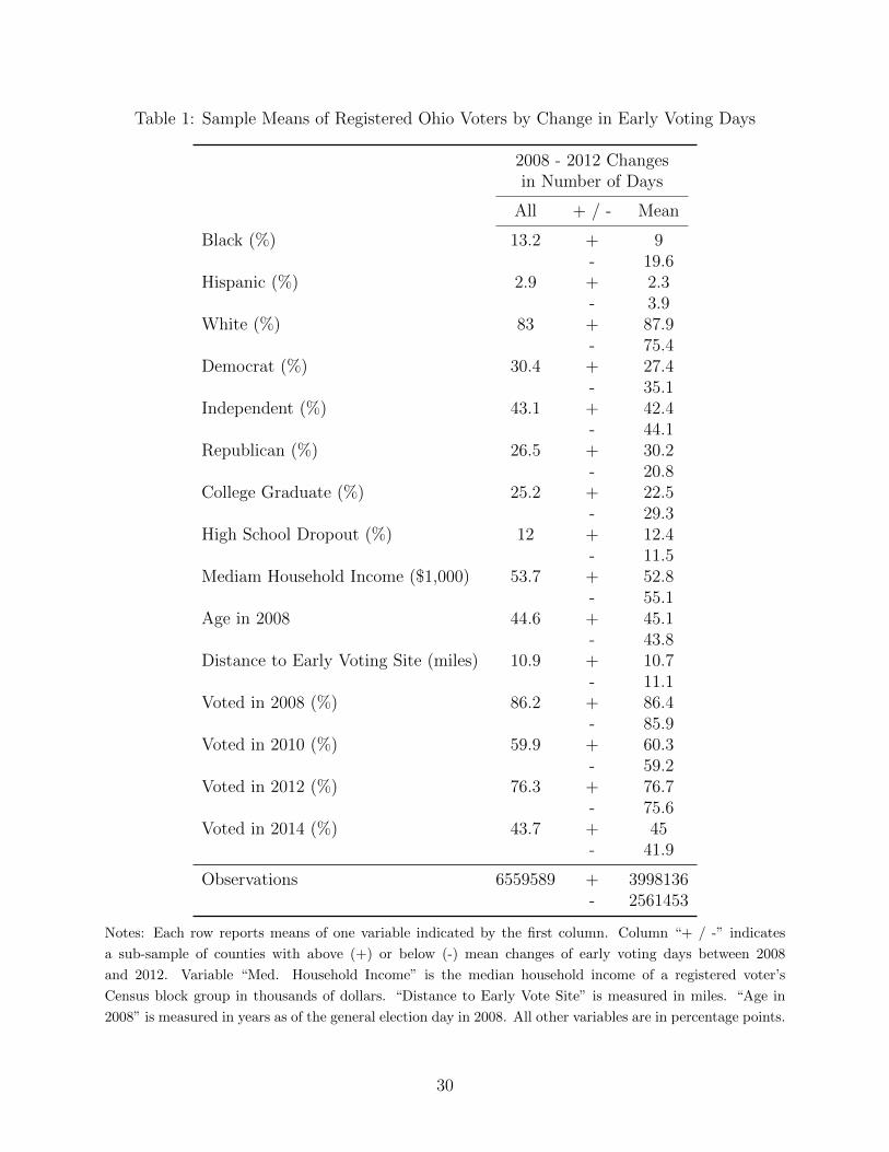
Table 1: Sample Means of Registered Ohio Voters by Change in Early Voting Days

2008 - 2012 Changesin Number of Days

All + / - Mean

Black (%) 13.2 + 9- 19.6

Hispanic (%) 2.9 + 2.3- 3.9

White (%) 83 + 87.9- 75.4

Democrat (%) 30.4 + 27.4- 35.1

Independent (%) 43.1 + 42.4- 44.1

Republican (%) 26.5 + 30.2- 20.8

College Graduate (%) 25.2 + 22.5- 29.3

High School Dropout (%) 12 + 12.4- 11.5

Mediam Household Income ($1,000) 53.7 + 52.8- 55.1

Age in 2008 44.6 + 45.1- 43.8

Distance to Early Voting Site (miles) 10.9 + 10.7- 11.1

Voted in 2008 (%) 86.2 + 86.4- 85.9

Voted in 2010 (%) 59.9 + 60.3- 59.2

Voted in 2012 (%) 76.3 + 76.7- 75.6

Voted in 2014 (%) 43.7 + 45- 41.9

Observations 6559589 + 3998136- 2561453

Notes: Each row reports means of one variable indicated by the first column. Column “+ / -” indicates

a sub-sample of counties with above (+) or below (-) mean changes of early voting days between 2008

and 2012. Variable “Med. Household Income” is the median household income of a registered voter’s

Census block group in thousands of dollars. “Distance to Early Vote Site” is measured in miles. “Age in

2008” is measured in years as of the general election day in 2008. All other variables are in percentage points.

30

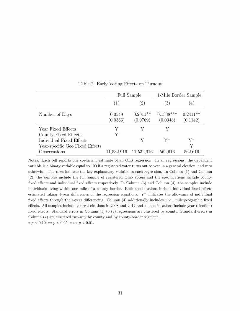
Table 2: Early Voting Effects on Turnout

Full Sample 1-Mile Border Sample

(1) (2) (3) (4)

Number of Days 0.0549 0.2011** 0.1338*** 0.2411**(0.0366) (0.0769) (0.0348) (0.1142)

Year Fixed Effects Y Y YCounty Fixed Effects YIndividual Fixed Effects Y Y− Y−

Year-specific Geo Fixed Effects YObservations 11,532,916 11,532,916 562,616 562,616

Notes: Each cell reports one coefficient estimate of an OLS regression. In all regressions, the dependent

variable is a binary variable equal to 100 if a registered voter turns out to vote in a general election; and zero

otherwise. The rows indicate the key explanatory variable in each regression. In Column (1) and Column

(2), the samples include the full sample of registered Ohio voters and the specifications include county

fixed effects and individual fixed effects respectively. In Column (3) and Column (4), the samples include

individuals living within one mile of a county border. Both specifications include individual fixed effects

estimated taking 4-year differences of the regression equations. Y− indicates the allowance of individual

fixed effects through the 4-year differencing. Column (4) additionally includes 1 × 1 mile geographic fixed

effects. All samples include general elections in 2008 and 2012 and all specifications include year (election)

fixed effects. Standard errors in Column (1) to (3) regressions are clustered by county. Standard errors in

Column (4) are clustered two-way by county and by county-border segment.

∗ p < 0.10; ∗∗ p < 0.05; ∗ ∗ ∗ p < 0.01.

31

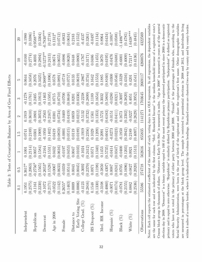
Tab

le3:

Tes

tsof

Cov

aria

tes

Bal

ance

by

Are

aof

Geo

Fix

edE

ffec

ts

0.1

0.5

11.

52

35

1020

Indep

enden

t0.

1951

0.36

17*

0.10

010.

0741

0.19

19-0

.127

80.

0644

-0.0

160

-0.1

980

(0.2

575)

(0.2

063)

(0.2

114)

(0.2

189)

(0.3

610)

(0.1

761)

(0.3

458)

(0.2

774)

(0.3

386)

Rep

ublica

n-0

.116

1-0

.275

6*0.

0057

0.03

01-0

.080

10.

2405

0.20

760.

4693

0.95

88**

*(0

.223

0)(0

.156

5)(0

.158

4)(0

.190

9)(0

.305

3)(0

.191

3)(0

.342

5)(0

.289

4)(0

.330

4)D

emocr

at-0

.107

2-0

.265

3*-0

.216

4-0

.195

0-0

.256

3-0

.146

3-0

.388

9**

-0.5

273*

*-0

.783

0***

(0.2

171)

(0.1

528)

(0.1

531)

(0.1

402)

(0.2

167)

(0.1

505)

(0.1

896)

(0.2

413)

(0.2

718)

Age

in20

08-0

.052

2-0

.006

70.

0432

0.04

190.

0381

0.07

150.

0578

0.06

740.

1312

*(0

.114

2)(0

.063

3)(0

.061

6)(0

.085

9)(0

.073

4)(0

.071

0)(0

.089

1)(0

.065

5)(0

.071

2)F

emal

e0.

2655

*-0

.035

9-0

.019

7-0

.000

1-0

.046

9-0

.070

0-0

.071

8-0

.088

6-0

.083

3(0

.146

3)(0

.051

4)(0

.045

3)(0

.051

5)(0

.041

9)(0

.064

8)(0

.075

7)(0

.062

0)(0

.063

4)D

ista

nce

to0.

0009

0.00

430.

0047

0.01

190.

0059

0.02

010.

0133

0.04

480.

2183

Ear

lyV

otin

gSit

e(0

.000

6)(0

.004

5)(0

.010

3)(0

.018

9)(0

.021

2)(0

.033

6)(0

.061

9)(0

.080

0)(0

.155

2)C

olle

geG

rad.

(%)

-0.4

123

-0.3

692

-0.1

024

-0.1

919

-0.5

132

-0.2

238

-0.2

867

-0.1

767

-0.4

537

(0.2

816)

(0.2

370)

(0.2

412)

(0.2

356)

(0.3

732)

(0.2

899)

(0.3

734)

(0.3

171)

(0.3

261)

HS

Dro

pou

t(%

)0.

1548

0.09

710.

0571

0.10

290.

1561

0.11

890.

1642

0.04

86-0

.049

7(0

.133

0)(0

.119

8)(0

.134

0)(0

.120

9)(0

.135

3)(0

.165

4)(0

.155

3)(0

.145

5)(0

.113

4)M

ed.

HH

.In

com

e-0

.310

8-0

.385

00.

1453

0.20

91-0

.572

10.

3032

0.18

850.

3870

0.89

64(0

.406

0)(0

.430

7)(0

.573

5)(0

.604

1)(0

.618

3)(0

.580

4)(0

.816

0)(0

.619

5)(0

.643

4)H

ispan

ic(%

)-0

.007

10.

0087

-0.0

414

-0.0

273

-0.0

151

-0.0

280

-0.0

300

-0.0

476

-0.1

091*

(0.0

174)

(0.0

241)

(0.0

347)

(0.0

323)

(0.0

411)

(0.0

321)

(0.0

546)

(0.0

488)

(0.0

588)

Bla

ck(%

)-0

.078

10.

0705

-0.0

400

-0.1

850

0.16

73-0

.369

7-0

.332

9-0

.600

1-1

.448

6***

(0.2

155)

(0.1

696)

(0.1

203)

(0.3

942)

(0.2

302)

(0.3

820)

(0.4

316)

(0.4

009)

(0.4

785)

Whit

e(%

)0.

0882

-0.0

827

0.09

210.

2189

-0.0

227

0.40

510.

4201

0.72

11*

1.64

38**

*(0

.253

6)(0

.202

0)(0

.151

3)(0

.409

7)(0

.262

9)(0

.395

2)(0

.454

1)(0

.413

6)(0

.484

5)

Obse

rvat

ions

5558

627

4718

5626

1685

5835

1141

271

1703

645

2669

117

4260

076

4322

569

Not

es:

Eac

hce

llre

por

tsth

ees

tim

ated

coeffi

cien

tof

the

nu

mb

erof

earl

yvo

tin

gday

sin

an

OL

Sre

gre

ssio

n.

Inall

regre

ssio

ns,

the

dep

end

ent

vari

ab

les

are

the

sam

efo

rea

chro

wan

dar

ein

dic

ated

by

the

firs

tco

lum

n.

“M

ed.

Hou

seh

old

Inco

me”

isth

em

edia

nh

ou

seh

old

inco

me

of

are

gis

tere

dvo

ter’

s

Cen

sus

blo

ckgr

oup

inth

ousa

nd

sof

dol

lars

.“D

ista

nce

toE

arl

yV

ote

Sit

e”is

mea

sure

din

mil

es.

“A

ge

in2008”

inm

easu

red

inye

ars

as

of

the

gen

eral

elec

tion

day

in20

08.

“Dem

ocr

at”

isa

bin

ary

vari

ab

leeq

ual

to100

ifth

em

ost

rece

nt

pri

mary

the

regis

tere

dp

art

icip

ate

din

sin

ce2000

isa

dem

ocr

ati

c

pri

mar

yan

dis

equ

alto

zero

other

wis

e.“R

epu

bli

can

”is

sim

ilarl

yd

efin

edby

Rep

ub

lica

np

rim

ary

part

icip

ati

on

.“In

dep

end

ent”

isd

efin

edas

regis

tere

d

vote

rsw

ho

hav

en

otvo

ted

inth

ep

rim

ary

ofei

ther

part

yb

etw

een

2000

an

d2008.

“F

emale

”is

the

per

centa

ges

of

fem

ale

sw

ho,

acc

ord

ing

toth

e

Soci

alS

ecu

rity

Ad

min

istr

atio

n,

wer

eb

orn

inth

eye

ar

of

bir

thof

the

regis

trant

an

dsh

are

the

regis

trant’

sfi

rst

nam

e.O

ther

dem

ogra

ph

icva

riable

s

are

mea

sure

din

per

centa

ges

atth

eblo

ckgr

oup

leve

l.T

he

sam

ple

isre

stri

cted

top

resi

den

tial

elec

tion

sin

2008

an

d2012,

an

din

div

idu

als

livin

g

wit

hink

mil

esof

aco

unty

bor

der

,w

her

ek

isin

dic

ate

dby

the

colu

mn

hea

din

gs.

Sta

nd

ard

erro

rsare

clu

ster

edtw

o-w

ayby

cou

nty

an

dby

cou

nty

-bord

er.

32

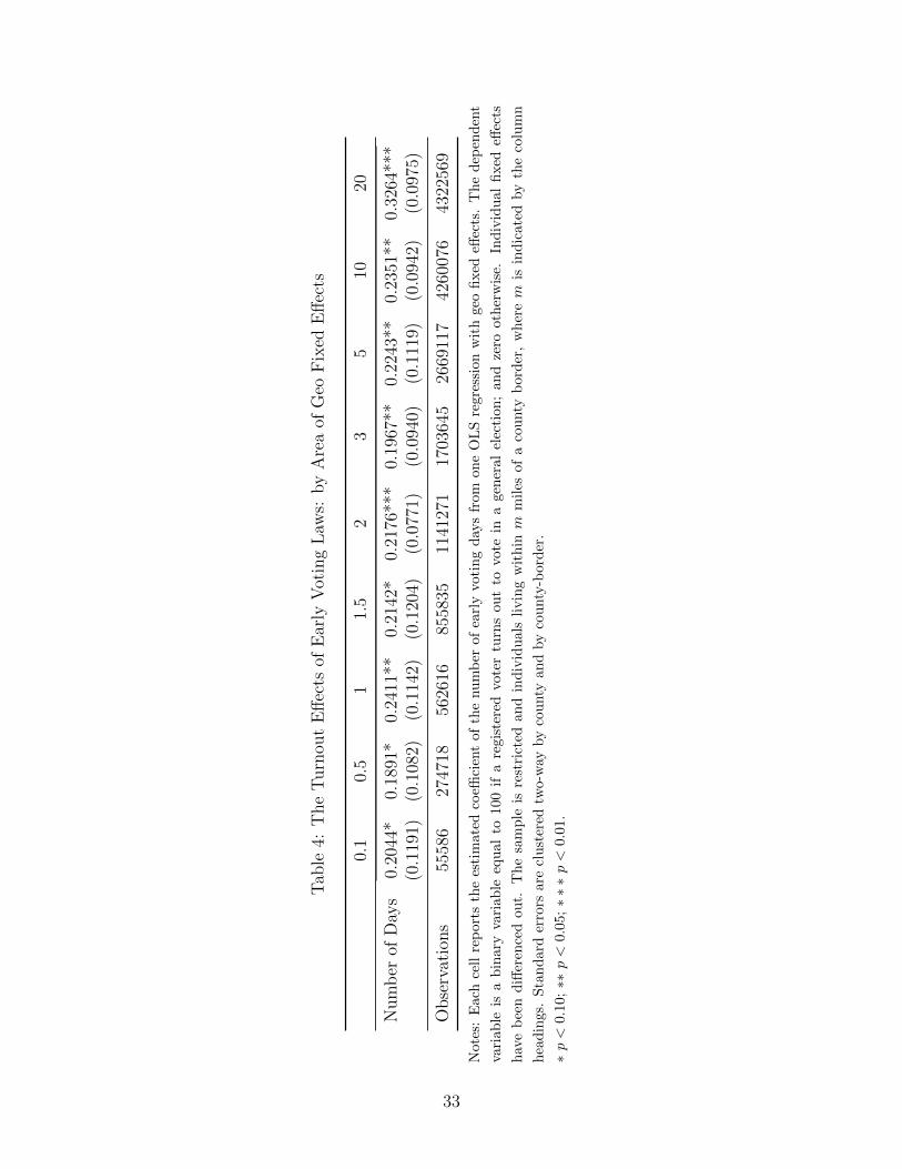
Tab

le4:

The

Turn

out

Eff

ects

ofE

arly

Vot

ing

Law

s:by

Are

aof

Geo

Fix

edE

ffec

ts

0.1

0.5

11.

52

35

1020

Num

ber

ofD

ays

0.20

44*

0.18

91*

0.24

11**

0.21

42*

0.21

76**

*0.

1967

**0.

2243

**0.

2351

**0.

3264

***

(0.1

191)

(0.1

082)

(0.1

142)

(0.1

204)

(0.0

771)

(0.0

940)

(0.1

119)

(0.0

942)

(0.0

975)

Obse

rvat

ions

5558

627

4718

5626

1685

5835

1141

271

1703

645

2669

117

4260

076

4322

569

Not

es:

Eac

hce

llre

por

tsth

ees

tim

ated

coeffi

cien

tof

the

nu

mb

erof

earl

yvo

tin

gd

ays

from

on

eO

LS

regre

ssio

nw

ith

geo

fixed

effec

ts.

Th

ed

epen

den

t

vari

able

isa

bin

ary

vari

able

equ

alto

100

ifa

regis

tere

dvote

rtu

rns

ou

tto

vote

ina

gen

eral

elec

tion

;an

dze

rooth

erw

ise.

Ind

ivid

ual

fixed

effec

ts

hav

eb

een

diff

eren

ced

out.

Th

esa

mp

leis

rest

rict

edan

din

div

iduals

livin

gw

ith

inm

mil

esof

aco

unty

bord

er,

wh

erem

isin

dic

ate

dby

the

colu

mn

hea

din

gs.

Sta

nd

ard

erro

rsar

ecl

ust

ered

two-

way

by

cou

nty

an

dby

cou

nty

-bord

er.

∗p<

0.10

;∗∗

p<

0.05

;∗∗∗p<

0.0

1.

33

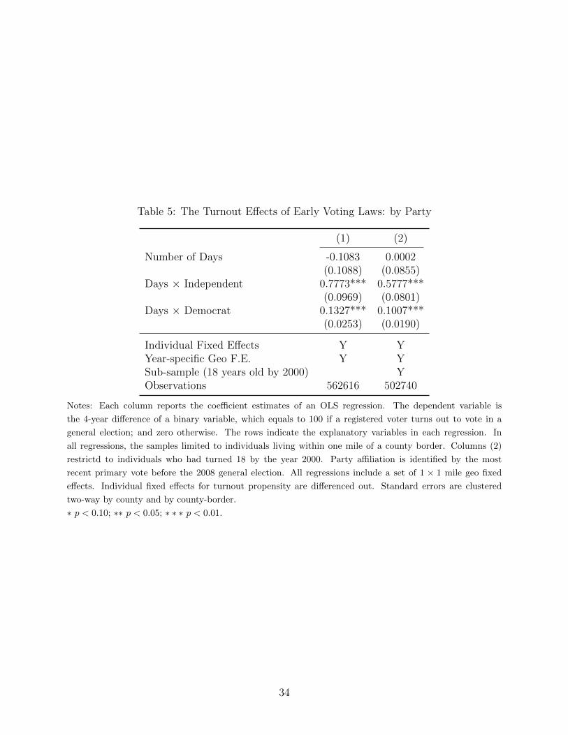
Table 5: The Turnout Effects of Early Voting Laws: by Party

(1) (2)

Number of Days -0.1083 0.0002(0.1088) (0.0855)

Days × Independent 0.7773*** 0.5777***(0.0969) (0.0801)

Days × Democrat 0.1327*** 0.1007***(0.0253) (0.0190)

Individual Fixed Effects Y YYear-specific Geo F.E. Y YSub-sample (18 years old by 2000) YObservations 562616 502740

Notes: Each column reports the coefficient estimates of an OLS regression. The dependent variable is

the 4-year difference of a binary variable, which equals to 100 if a registered voter turns out to vote in a

general election; and zero otherwise. The rows indicate the explanatory variables in each regression. In

all regressions, the samples limited to individuals living within one mile of a county border. Columns (2)

restrictd to individuals who had turned 18 by the year 2000. Party affiliation is identified by the most

recent primary vote before the 2008 general election. All regressions include a set of 1 × 1 mile geo fixed

effects. Individual fixed effects for turnout propensity are differenced out. Standard errors are clustered

two-way by county and by county-border.

∗ p < 0.10; ∗∗ p < 0.05; ∗ ∗ ∗ p < 0.01.

34

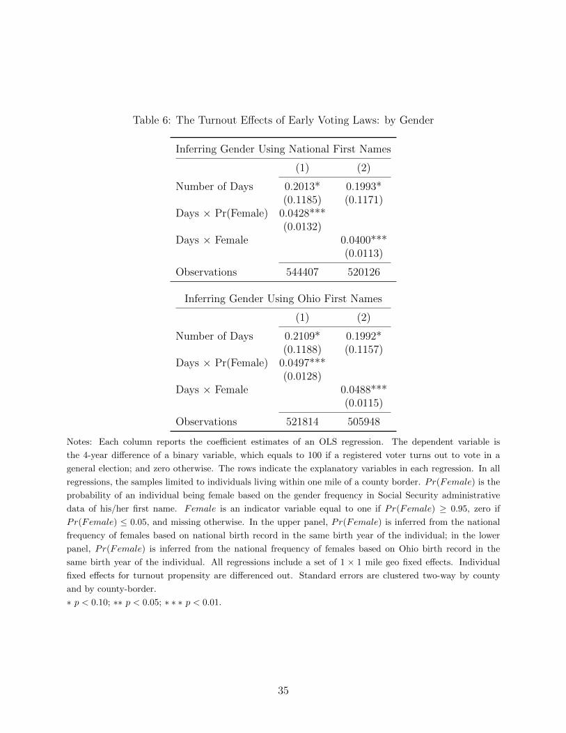
Table 6: The Turnout Effects of Early Voting Laws: by Gender

Inferring Gender Using National First Names

(1) (2)

Number of Days 0.2013* 0.1993*(0.1185) (0.1171)

Days × Pr(Female) 0.0428***(0.0132)

Days × Female 0.0400***(0.0113)

Observations 544407 520126

Inferring Gender Using Ohio First Names

(1) (2)

Number of Days 0.2109* 0.1992*(0.1188) (0.1157)

Days × Pr(Female) 0.0497***(0.0128)

Days × Female 0.0488***(0.0115)

Observations 521814 505948

Notes: Each column reports the coefficient estimates of an OLS regression. The dependent variable is

the 4-year difference of a binary variable, which equals to 100 if a registered voter turns out to vote in a

general election; and zero otherwise. The rows indicate the explanatory variables in each regression. In all

regressions, the samples limited to individuals living within one mile of a county border. Pr(Female) is the

probability of an individual being female based on the gender frequency in Social Security administrative

data of his/her first name. Female is an indicator variable equal to one if Pr(Female) ≥ 0.95, zero if

Pr(Female) ≤ 0.05, and missing otherwise. In the upper panel, Pr(Female) is inferred from the national

frequency of females based on national birth record in the same birth year of the individual; in the lower

panel, Pr(Female) is inferred from the national frequency of females based on Ohio birth record in the

same birth year of the individual. All regressions include a set of 1 × 1 mile geo fixed effects. Individual

fixed effects for turnout propensity are differenced out. Standard errors are clustered two-way by county

and by county-border.

∗ p < 0.10; ∗∗ p < 0.05; ∗ ∗ ∗ p < 0.01.

35

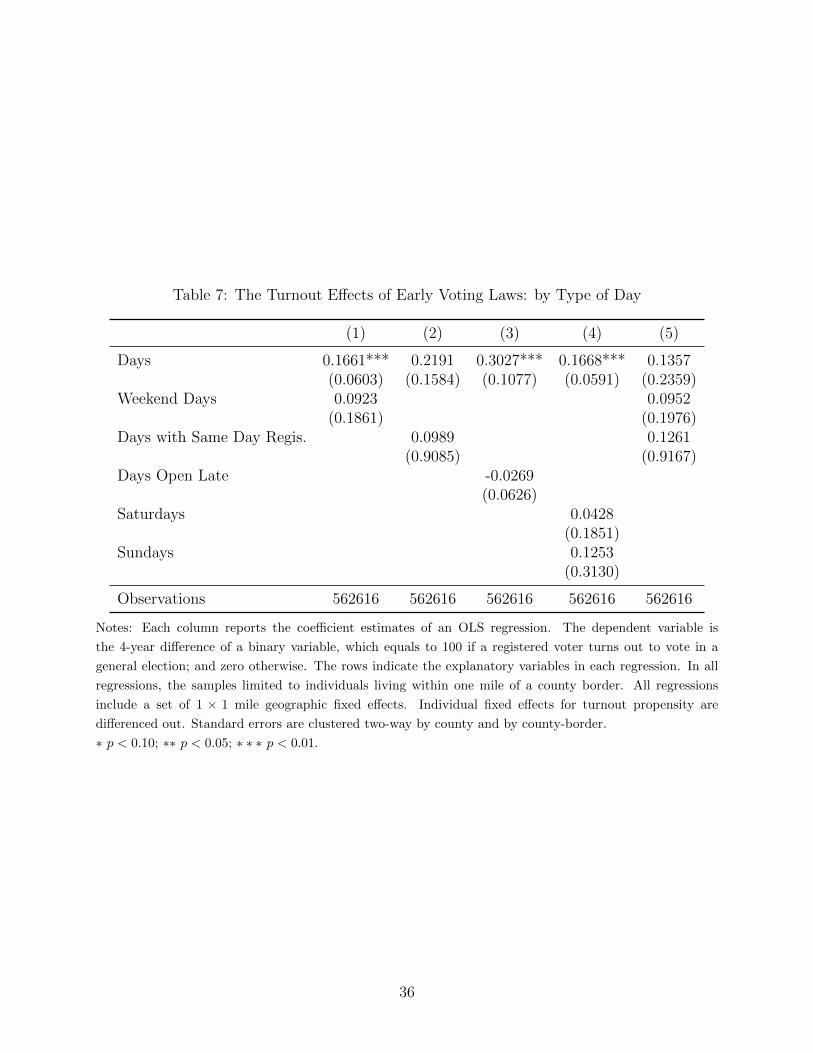
Table 7: The Turnout Effects of Early Voting Laws: by Type of Day

(1) (2) (3) (4) (5)

Days 0.1661*** 0.2191 0.3027*** 0.1668*** 0.1357(0.0603) (0.1584) (0.1077) (0.0591) (0.2359)

Weekend Days 0.0923 0.0952(0.1861) (0.1976)

Days with Same Day Regis. 0.0989 0.1261(0.9085) (0.9167)

Days Open Late -0.0269(0.0626)

Saturdays 0.0428(0.1851)

Sundays 0.1253(0.3130)

Observations 562616 562616 562616 562616 562616

Notes: Each column reports the coefficient estimates of an OLS regression. The dependent variable is

the 4-year difference of a binary variable, which equals to 100 if a registered voter turns out to vote in a

general election; and zero otherwise. The rows indicate the explanatory variables in each regression. In all

regressions, the samples limited to individuals living within one mile of a county border. All regressions

include a set of 1 × 1 mile geographic fixed effects. Individual fixed effects for turnout propensity are

differenced out. Standard errors are clustered two-way by county and by county-border.

∗ p < 0.10; ∗∗ p < 0.05; ∗ ∗ ∗ p < 0.01.

36

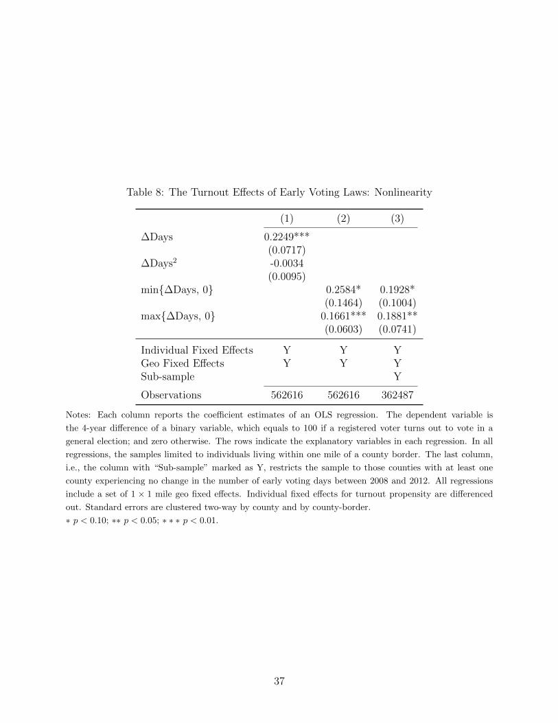
Table 8: The Turnout Effects of Early Voting Laws: Nonlinearity

(1) (2) (3)

∆Days 0.2249***(0.0717)

∆Days2 -0.0034(0.0095)

min{∆Days, 0} 0.2584* 0.1928*(0.1464) (0.1004)

max{∆Days, 0} 0.1661*** 0.1881**(0.0603) (0.0741)

Individual Fixed Effects Y Y YGeo Fixed Effects Y Y YSub-sample Y

Observations 562616 562616 362487

Notes: Each column reports the coefficient estimates of an OLS regression. The dependent variable is

the 4-year difference of a binary variable, which equals to 100 if a registered voter turns out to vote in a

general election; and zero otherwise. The rows indicate the explanatory variables in each regression. In all

regressions, the samples limited to individuals living within one mile of a county border. The last column,

i.e., the column with “Sub-sample” marked as Y, restricts the sample to those counties with at least one

county experiencing no change in the number of early voting days between 2008 and 2012. All regressions

include a set of 1 × 1 mile geo fixed effects. Individual fixed effects for turnout propensity are differenced

out. Standard errors are clustered two-way by county and by county-border.

∗ p < 0.10; ∗∗ p < 0.05; ∗ ∗ ∗ p < 0.01.

37

Table 9: Changes of Republican Seats and Electoral College Votes under Hypothetical Stan-dardized Early Voting

Observed Republican Standardized Early Voting

Election Type Year Seats / Electoral Votes 0 Days 23 Days 46 Days

President 2012 332/538 0 0 -15President 2016 304/538 10 -65* -75*

Senate 2012 51/100 1 -1* -1*Senate 2016 52/100 0 -1 -3*

House 2012 234/435 5 -4 -10House 2016 241/435 1 0 -3

Notes: Each element of the columns under the heading “Standardized Early Voting” reports the simulated

impact of national legislation requiring 0, 23 and 46 days of early voting respectively. Impacts are computed

using estimates by party and election type from Ohio but are applied nationally. For Senate and House

rows, numbers reflect the change in the number of seats to the Republican party. For the President row,

numbers reflect the change in the number of electoral votes to the Republican party. Positive numbers

indicate a net shift in favor of the Republican party and negative numbers indicate a net shift in favor

of the Democratic party. ∗ indicates a change of majority control in the congress or majority of electoral votes.

38

Figure 1: Changes in Early Voting Days

Cincinnati

Cleveland

Columbus

[-9, -5](-5, 0)0415

2008 - 2012

39

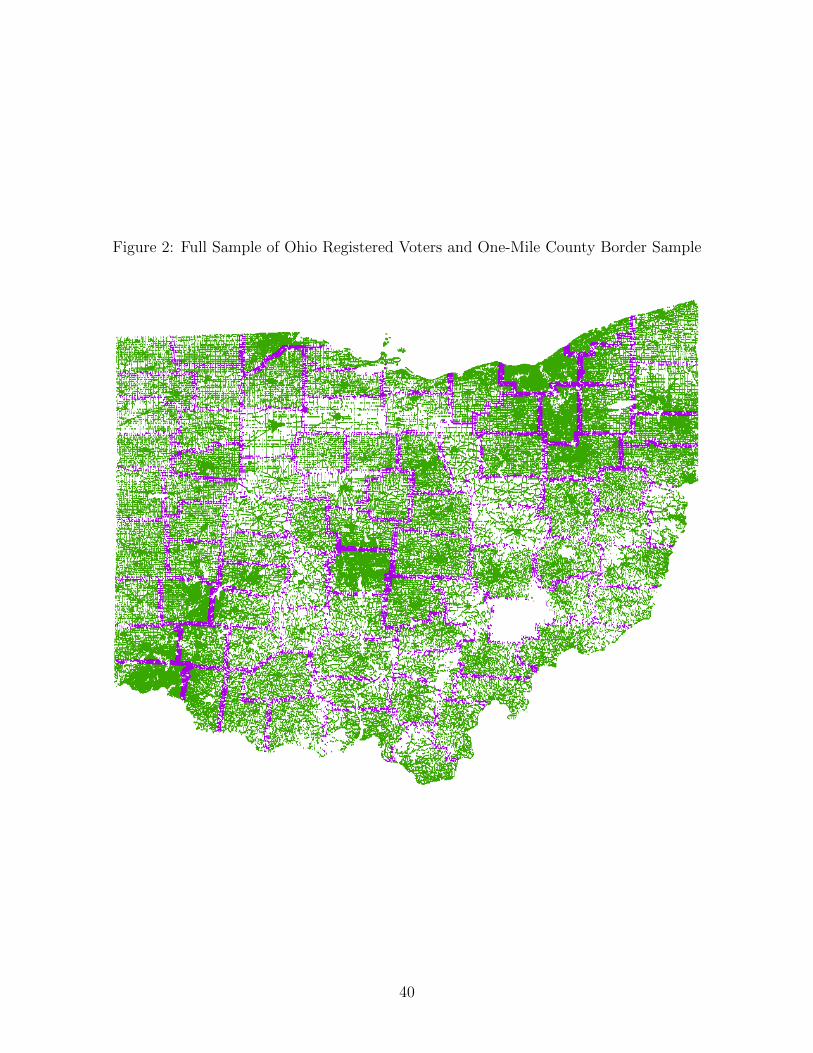
Figure 2: Full Sample of Ohio Registered Voters and One-Mile County Border Sample

40

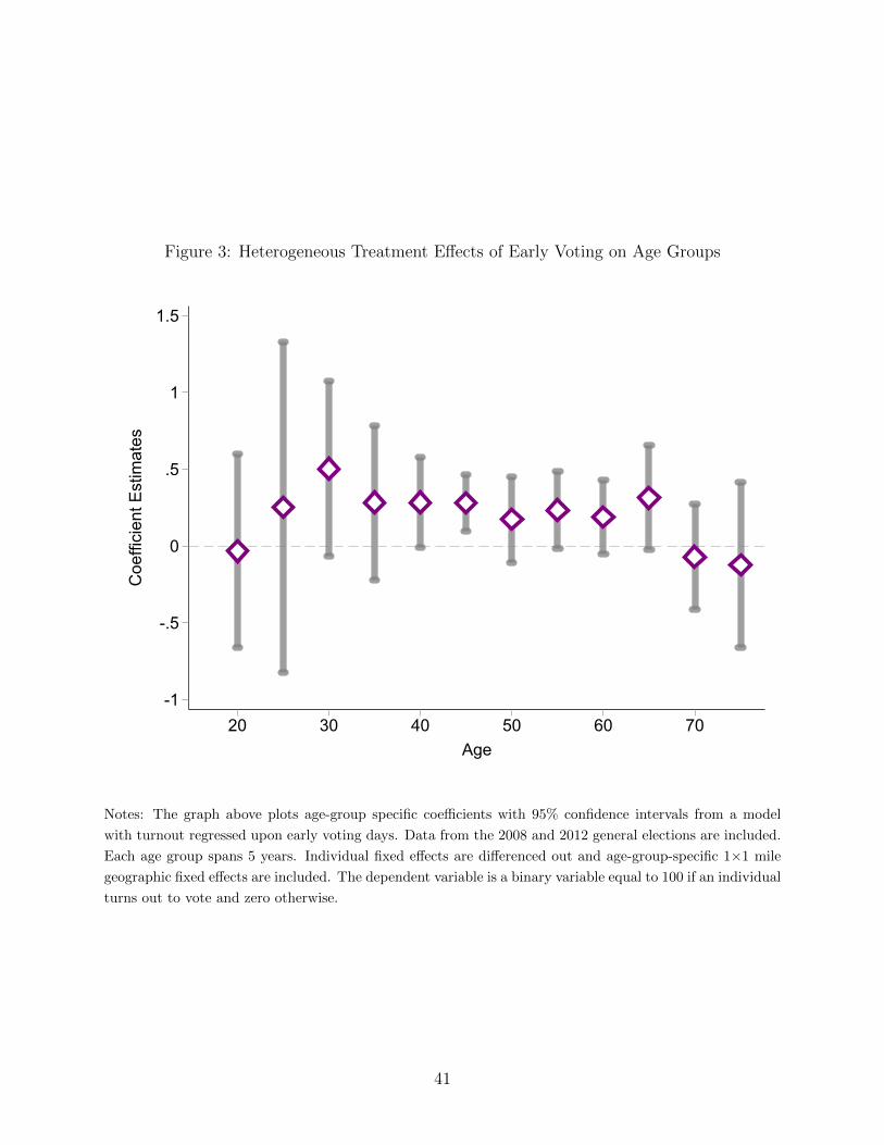
Figure 3: Heterogeneous Treatment Effects of Early Voting on Age Groups

-1

-.5

0

.5

1

1.5

Coe

ffici

ent E

stim

ates

20 30 40 50 60 70Age

Notes: The graph above plots age-group specific coefficients with 95% confidence intervals from a model

with turnout regressed upon early voting days. Data from the 2008 and 2012 general elections are included.

Each age group spans 5 years. Individual fixed effects are differenced out and age-group-specific 1×1 mile

geographic fixed effects are included. The dependent variable is a binary variable equal to 100 if an individual

turns out to vote and zero otherwise.

41

Appendix

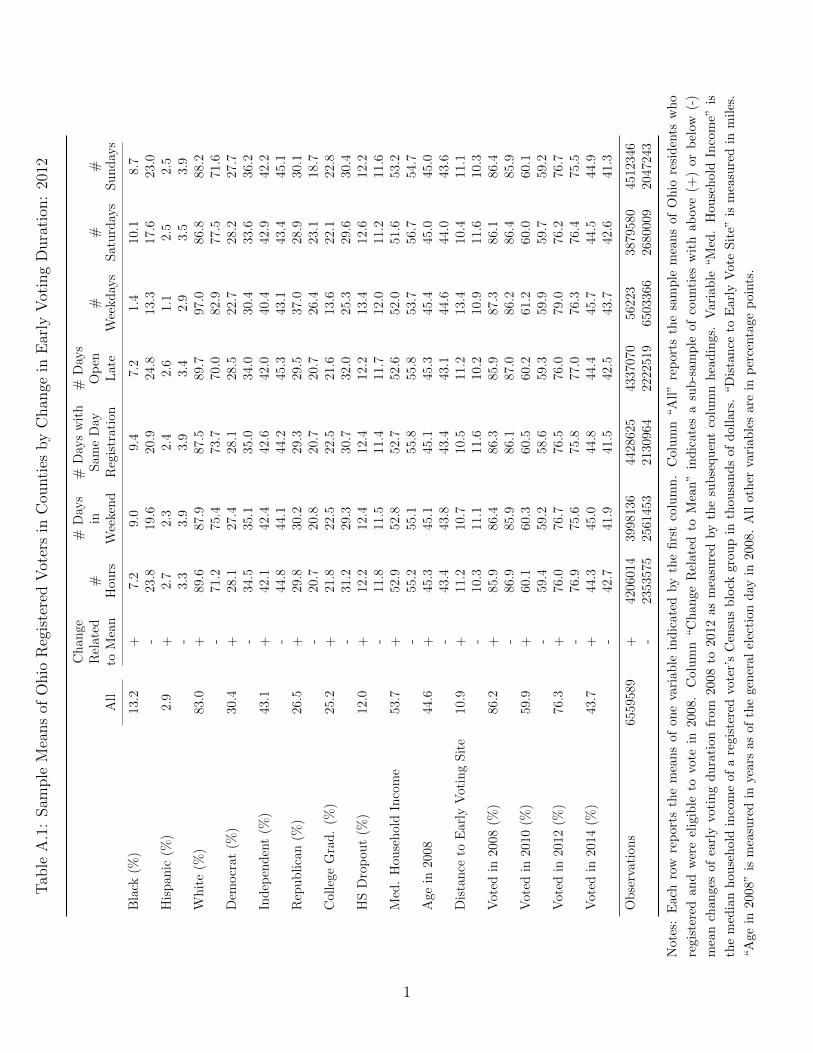
Tab

leA

.1:

Sam

ple

Mea

ns

ofO

hio

Reg

iste

red

Vot

ers

inC

ounti

esby

Chan

gein

Ear

lyV

otin

gD

ura

tion

:20

12

Ch

ange

#D

ays

#D

ays

wit

h#

Day

sR

elat

ed#

inS

ame

Day

Op

en#

##

All

toM

ean

Hou

rsW

eeke

nd

Reg

istr

atio

nL

ate

Wee

kd

ays

Sat

urd

ays

Su

nd

ays

Bla

ck(%

)13

.2+

7.2

9.0

9.4

7.2

1.4

10.1

8.7

-23

.819

.620

.924

.813

.317

.623

.0H

isp

anic

(%)

2.9

+2.

72.

32.

42.

61.

12.

52.

5-

3.3

3.9

3.9

3.4

2.9

3.5

3.9

Wh

ite

(%)

83.0

+89

.687

.987

.589

.797

.086

.888

.2-

71.2

75.4

73.7

70.0

82.9

77.5

71.6

Dem

ocr

at(%

)30

.4+

28.1

27.4

28.1

28.5

22.7

28.2

27.7

-34

.535

.135

.034

.030

.433

.636

.2In

dep

end

ent

(%)

43.1

+42

.142

.442

.642

.040

.442

.942

.2-

44.8

44.1

44.2

45.3

43.1

43.4

45.1

Rep

ub

lica

n(%

)26

.5+

29.8

30.2

29.3

29.5

37.0

28.9

30.1

-20

.720

.820

.720

.726

.423

.118

.7C

olle

geG

rad

.(%

)25

.2+

21.8

22.5

22.5

21.6

13.6

22.1

22.8

-31

.229

.330

.732

.025

.329

.630

.4H

SD

rop

out

(%)

12.0

+12

.212

.412

.412

.213

.412

.612

.2-

11.8

11.5

11.4

11.7

12.0

11.2

11.6

Med

.H

ouse

hol

dIn

com

e53

.7+

52.9

52.8

52.7

52.6

52.0

51.6

53.2

-55

.255

.155

.855

.853

.756

.754

.7A

gein

2008

44.6

+45

.345

.145

.145

.345

.445

.045

.0-

43.4

43.8

43.4

43.1

44.6

44.0

43.6

Dis

tan

ceto

Ear

lyV

otin

gS

ite

10.9

+11

.210

.710

.511

.213

.410

.411

.1-

10.3

11.1

11.6

10.2

10.9

11.6

10.3

Vot

edin

2008

(%)

86.2

+85

.986

.486

.385

.987

.386

.186

.4-

86.9

85.9

86.1

87.0

86.2

86.4

85.9

Vot

edin

2010

(%)

59.9

+60

.160

.360

.560

.261

.260

.060

.1-

59.4

59.2

58.6

59.3

59.9

59.7

59.2

Vot

edin

2012

(%)

76.3

+76

.076

.776

.576

.079

.076

.276

.7-

76.9

75.6

75.8

77.0

76.3

76.4

75.5

Vot

edin

2014

(%)

43.7

+44

.345

.044

.844

.445

.744

.544

.9-

42.7

41.9

41.5

42.5

43.7

42.6

41.3

Ob

serv

atio

ns

6559

589

+42

0601

439

9813

644

2862

543

3707

056

223

3879

580

4512

346

-23

5357

525

6145

321

3096

422

2251

965

0336

626

8000

920

4724

3

Not

es:

Eac

hro

wre

por

tsth

em

ean

sof

one

vari

ab

lein

dic

ate

dby

the

firs

tco

lum

n.

Colu

mn

“A

ll”

rep

ort

sth

esa

mp

lem

ean

sof

Oh

iore

sid

ents

wh

o

regi

ster

edan

dw

ere

elig

ible

tovo

tein

2008

.C

olu

mn

“C

han

ge

Rel

ate

dto

Mea

n”

ind

icate

sa

sub

-sam

ple

of

cou

nti

esw

ith

ab

ove

(+)

or

bel

ow(-

)

mea

nch

ange

sof

earl

yvo

tin

gd

ura

tion

from

2008

to2012

as

mea

sure

dby

the

sub

sequ

ent

colu

mn

hea

din

gs.

Vari

ab

le“M

ed.

Hou

seh

old

Inco

me”

is

the

med

ian

hou

seh

old

inco

me

ofa

regi

ster

edvo

ter’

sC

ensu

sb

lock

gro

up

inth

ou

san

ds

of

doll

ars

.“D

ista

nce

toE

arl

yV

ote

Sit

e”is

mea

sure

din

mil

es.

“Age

in20

08”

ism

easu

red

inye

ars

asof

the

gen

eral

elec

tion

day

in2008.

All

oth

erva

riab

les

are

inp

erce

nta

ge

poin

ts.

1

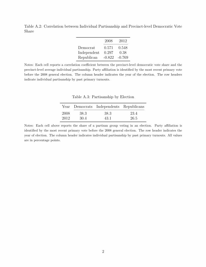
Table A.2: Correlation between Individual Partisanship and Precinct-level Democratic VoteShare

2008 2012

Democrat 0.571 0.548Independent 0.297 0.38Republican -0.822 -0.769

Notes: Each cell reports a correlation coefficient between the precinct-level democratic vote share and the

precinct-level average individual partisanship. Party affiliation is identified by the most recent primary vote

before the 2008 general election. The column header indicates the year of the election. The row headers

indicate individual partisanship by past primary turnouts.

Table A.3: Partisanship by Election

Year Democrats Independents Republicans

2008 38.3 38.3 23.42012 30.4 43.1 26.5

Notes: Each cell above reports the share of a partisan group voting in an election. Party affiliation is

identified by the most recent primary vote before the 2008 general election. The row header indicates the

year of election. The column header indicates individual partisanship by past primary turnouts. All values

are in percentage points.

2

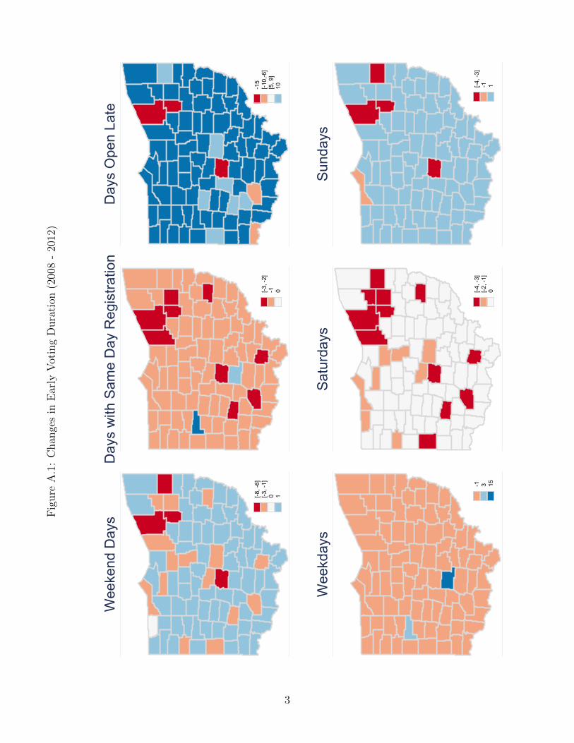
Fig

ure

A.1

:C

han

ges

inE

arly

Vot

ing

Dura

tion

(200

8-

2012

)

[-8, -

6][-3

, -1]

0 1

Wee

kend

Day

s

[-3, -

2]-1 0

Day

s w

ith S

ame

Day

Reg

istra

tion

-15

[-10,

-6]

[5, 9

]10

Day

s O

pen

Late

-1 3 15

Wee

kday

s

[-4, -

3][-2

, -1]

0

Satu

rday

s

[-4, -

3]-1 1

Sund

ays

3

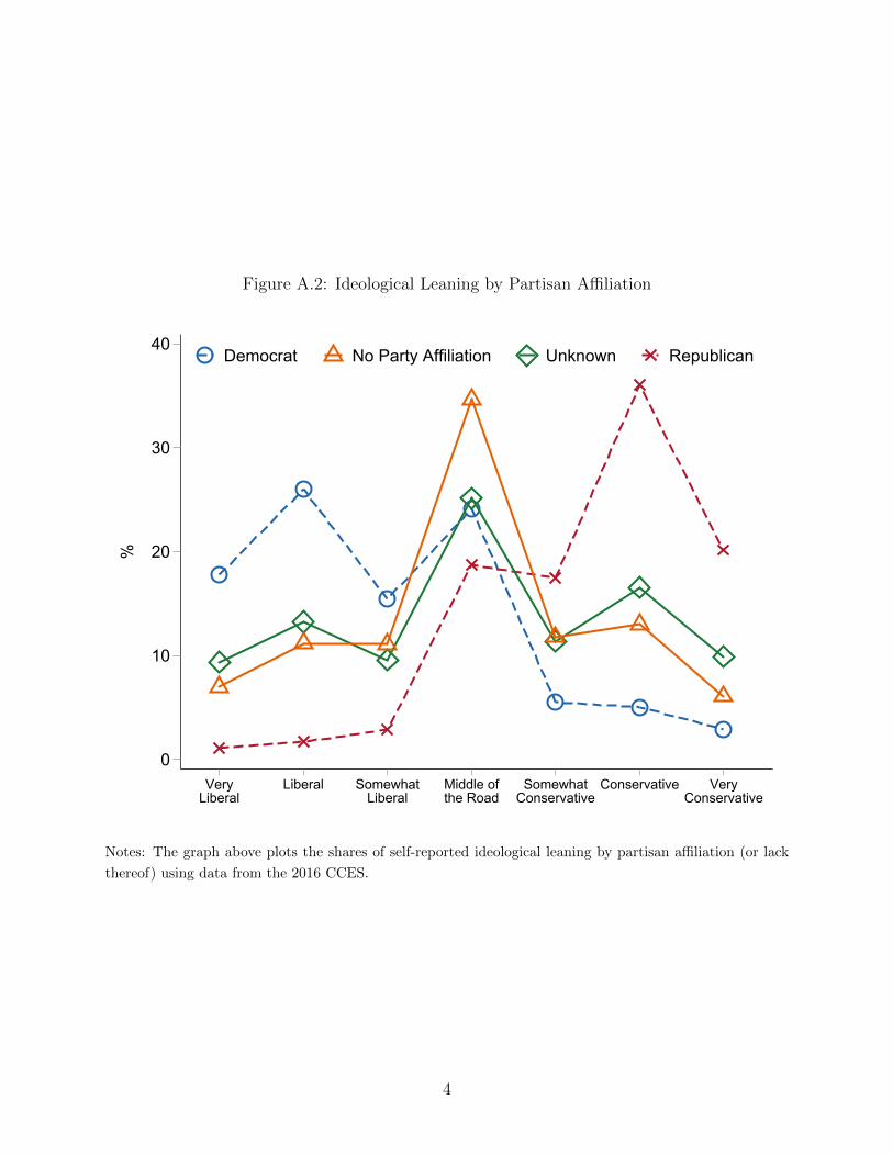
Figure A.2: Ideological Leaning by Partisan Affiliation

0

10

20

30

40

%

VeryLiberal

Liberal SomewhatLiberal

Middle ofthe Road

SomewhatConservative

Conservative VeryConservative

Democrat No Party Affiliation Unknown Republican

Notes: The graph above plots the shares of self-reported ideological leaning by partisan affiliation (or lack

thereof) using data from the 2016 CCES.

4

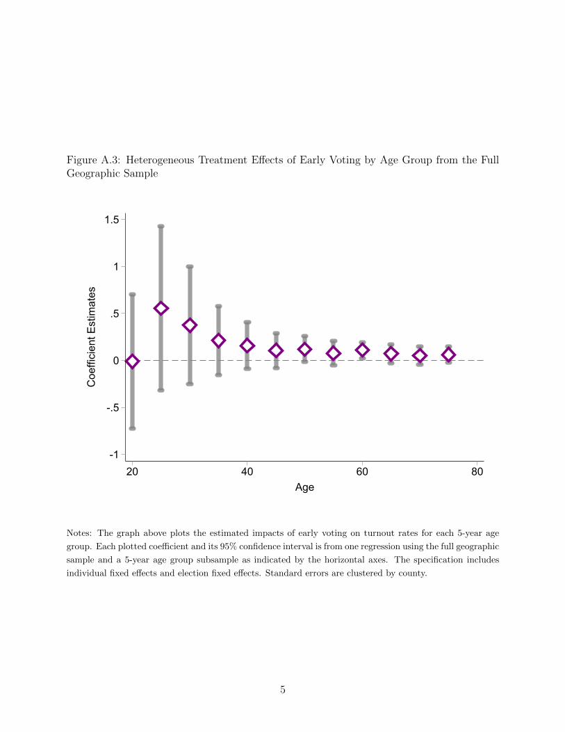
Figure A.3: Heterogeneous Treatment Effects of Early Voting by Age Group from the FullGeographic Sample

-1

-.5

0

.5

1

1.5

Coe

ffici

ent E

stim

ates

20 40 60 80Age

Notes: The graph above plots the estimated impacts of early voting on turnout rates for each 5-year age

group. Each plotted coefficient and its 95% confidence interval is from one regression using the full geographic

sample and a 5-year age group subsample as indicated by the horizontal axes. The specification includes

individual fixed effects and election fixed effects. Standard errors are clustered by county.

5

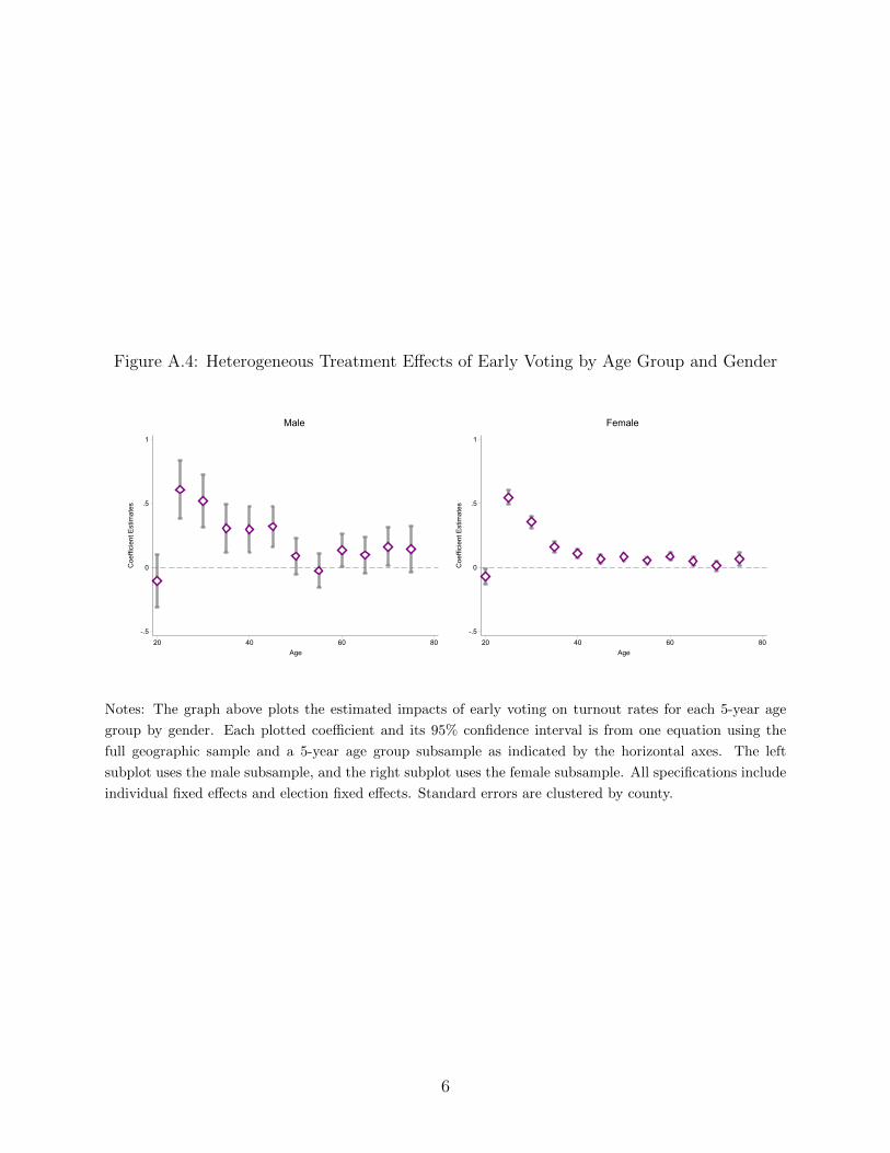
Figure A.4: Heterogeneous Treatment Effects of Early Voting by Age Group and Gender

-.5

0

.5

1

Coe

ffici

ent E

stim

ates

20 40 60 80Age

Male

-.5

0

.5

1

Coe

ffici

ent E

stim

ates

20 40 60 80Age

Female

Notes: The graph above plots the estimated impacts of early voting on turnout rates for each 5-year age

group by gender. Each plotted coefficient and its 95% confidence interval is from one equation using the

full geographic sample and a 5-year age group subsample as indicated by the horizontal axes. The left

subplot uses the male subsample, and the right subplot uses the female subsample. All specifications include

individual fixed effects and election fixed effects. Standard errors are clustered by county.

6