LCTP-19-08

Early-Universe Simulations of the Cosmological Axion

Malte Buschmann, Joshua W. Foster, and Benjamin R. SafdiLeinweber Center for Theoretical Physics, Department of Physics, University of Michigan, Ann Arbor, MI 48109

Ultracompact dark matter (DM) minihalos at masses at and below 10−12 M arise in axionDM models where the Peccei-Quinn (PQ) symmetry is broken after inflation. The minihalos arisefrom density perturbations that are generated from the non-trivial axion self interactions duringand shortly after the collapse of the axion-string and domain-wall network. We perform high-resolution simulations of this scenario starting at the epoch before the PQ phase transition andending at matter-radiation equality. We characterize the spectrum of primordial perturbations thatare generated and comment on implications for efforts to detect axion DM. We also measure theDM density at different simulated masses and argue that the correct DM density is obtained forma = 25.2 ± 11.0 µeV.

The quantum chromodynamics (QCD) axion is a well-motivated dark-matter (DM) candidate capable of pro-ducing the present-day abundance of DM while also re-solving the strong CP problem of the neutron electricdipole moment [1–7]. The axion is an ultralight pseudo-scalar particle whose mass primarily arises from the op-erator aGG/fa, with a the axion field, G the QCD field

strength, G its dual, and fa the axion decay constant.Below the QCD confinement scale, this operator gener-ates a potential for the axion; when the axion minimizesthis potential it dynamically removes the neutron electricdipole moment, thus solving the strong CP problem. Inthe process the axion acquires a mass ma ∼ Λ2

QCD/fa,with ΛQCD the QCD confinement scale. The standardultraviolet completion of the axion low-energy effectivefield theory is that the axion is a pseudo-Goldstone bosonof a symmetry, called the Peccei-Quinn (PQ) symmetry,which is broken at the scale fa [8–12].

The cosmology of the axion depends crucially on theordering of PQ symmetry breaking and inflation. Ifthe PQ symmetry is broken before or during inflation,then inflation produces homogeneous initial conditionsfor axion field and generically the cosmology is relativelystraightforward [13]. In this work we focus on the morecomplex scenario where the PQ symmetry is broken af-ter reheating. Immediately after PQ symmetry break-ing, the initial axion field is uncorrelated on scales largerthan the horizon, with neighboring Hubble patches com-ing into causal contact in the subsequent evolution of theUniverse. This leads to complicated dynamical phenom-ena, such as global axion strings, domain walls, and non-linear field configurations called oscillons (also referredto as axitons) [14–20].

We perform numerical simulations to evolve the axionfield from the epoch directly before PQ symmetry break-ing to directly after the QCD phase transition. Once thefield has entered the linear regime after the QCD phasetransition, we analytically evolve the free-field axion tomatter-radiation equality. The central motivations forthis work are to (i) quantify the spectrum of small-scaleultracompact minihalos that emerges through the non-trivial axion self-interactions and initial conditions, and(ii) to determine the ma that leads to the correct DM

density in this scenario.

The post-inflation PQ symmetry breaking cosmolog-ical scenario has been the subject of considerable nu-merical and analytic studies. It has been conjecturedthat this cosmology gives rise to ultra-dense compactDM minihalos with characteristic masses ∼10−13-10−11

M, though we show that the typical masses are actuallysmaller than this, and initial DM overdensities of orderunity [15–17, 20–23]. In this work we compute the mini-halo mass function precisely, combining state-of-the-artnumerical simulations with a self-consistent cosmologicalpicture. Understanding this mass function is importantas it affects the ways that we look for axions in this cos-mological scenario. For example, it has been claimed thatmicrolensing by minihalos and pulsar timing surveys [24]may constrain the post-inflation PQ symmetry breakingaxion scenario [23], but these analyses rely crucially onthe form of the mass function at high overdensities andmasses. The axion minihalos may also impact indirectefforts to detect axion DM through radio signatures [25–30].

A precise knowledge of the ma that gives the ob-served DM density is of critical importance for ax-ion direct detection experiments [31–41]. We findma = 25.2± 11.0 µeV, which is within range of e.g. theHAYSTAC program [35]. Our axion mass estimateis similar to that found in recent simulations [42] butdisagrees substantially with earlier semi-analytic esti-mates [43–49]. The minihalo mass function is also im-portant for interpreting the results of the laboratory ex-periments. If a large fraction of the energy density of DMis in compact minihalos, it is possible that the expectedDM density at Earth is quite low or highly time de-pendent, which means that direct detection experimentswould need to be more sensitive than previously thoughtor use an alternate observing strategy.

The original simulations that tried to estimate theminihalo mass function were performed in [16] on a gridof size 1003. Ref. [16] found oscillons (soliton-like oscil-latory solutions) that contribute to the high-overdensitytail of the mass function. Note that oscillons are analo-gous to the breather solutions found in the Sine-Gordonequation (see e.g. [50]). Recently [20] performed updated

arX

iv:1

906.

0096

7v1

[as

tro-

ph.C

O]

3 J

un 2

019

2

simulations on a grid of size 81923. Our results expand onand differ from those presented in [20] in many ways, suchas through our initial state that begins before the PQphase transition, measurement of the overall DM density,evolution to matter-radiation equality, and accounting ofnon-Gaussianities.Simulation setup: We begin our simulations with acomplex scalar PQ field Φ, with Lagrangian

LPQ =1

2|∂Φ|2 − λ

4

(|Φ|2 − f2

a

)2 − λT 2

6|Φ|2

−ma(T )2f2a [1− cos Arg(Φ)],

(1)

with T the temperature, λ the PQ quartic couplingstrength, and ma(T ) the temperature-dependent axionmass generated by QCD [51]. We fix λ = 1 for definite-ness, though this does not affect our final results. Theparametrization of the temperature-dependent mass isadopted from the leading-order term in the fit in [46].Explicitly, the axion mass is parametrized by

ma(T )2 = min

[αaΛ4

f2a (T/Λ)n

, m2a

], (2)

for αa = 1.68× 10−7, Λ = 400 MeV and n = 6.68,though in the Supplementary Material (SM) we consideralternate parameterizations. The growth of the massis truncated when it reaches its zero-temperature value,which occurs at T ≈ 100 MeV independent of the axiondecay constant. The zero-temperature mass is given byma ≈ 5.707× 10−5(1011 GeV/fa) eV [52].

For the PQ-epoch simulations we begin well before thebreaking of the PQ symmetry at a time when the PQfield is described by a thermal spectrum. The simula-tion is performed by evolving the equations of motion ona uniformly spaced grid of side-length LPQ = 8000 inunits of 1/(a1H1), with a1 (H1) the scale factor (Hubbleparameter) at the temperature when H1 = fa, at a res-olution of 10243 grid-sites. We use a standard leap-frogalgorithm in the kick-drift-kick form with an adaptivetime-step size and with the numerical Laplacian calcu-lated by the seven-point stencil. It is convenient to usethe rescaled conformal time η = η/η1, where η1 is theconformal time at which point H(η1) ≡ H1 = fa. Thesimulation begins at ηi = 0.0001 and proceeds with ini-tial time-step ∆ηi = 0.004 until η = 250, after whicha variable time-step calculated by ∆ηi(250/η) is used tomaintain temporal resolution of the oscillating PQ fields.Convergence was tested by re-running small time inter-vals of the simulation at smaller time steps. The PQ fieldsevolve from their initial thermal configuration until thePQ phase transition occurs at η ≈ 280, after which theradial mode |Φ/fa| acquires its vacuum expectation value(VEV). We simulate until ηf = 800 in order to proceedto a time at which fluctuations around the radial modeVEV have become highly damped.

Note that the difference in η between η = 1 and thePQ phase transition is proportional to

√mpl/fa, with

mpl the Planck mass. The actual choice of fa here does

not play an important role since we evolve the axion-string network into the scaling regime. In the left panelof Fig. 1 we show the final state of our simulation at thecompletion of the PQ simulation. The string network isseen in yellow, with the blue colors indicating regions ofhigher than average axion density. The length of the sim-ulation box at this point is around 8000/(a(ηf )H(ηf )),and we indeed find that there is around one string perHubble patch as would be expected in the scaling regime.

We use the final state of the PQ-epoch simulation asthe initial state in our QCD-epoch simulation. To do sowe assume that the axion-string network remains in thescaling regime between the two phase transitions (see,e.g., [47]). Recently [53] found evidence for a logarith-mic deviation to the scaling solution and we confirm thisbehavior in the SM. However, we perform tests to showthat this deviation to scaling likely has a minimal impacton both the minihalo mass function and on the DM den-sity, though we still assign a systematic uncertainty toour DM density estimate from the scaling violation.

Anticipating requiring greater spatial resolution forlate-times in our QCD simulation, we increased the reso-lution of our simulation to 20483 grid-sites with a nearest-neighbor interpolation algorithm. We re-interpreted thephysical dimensions of our box from side-length LPQ =8000 in PQ spatial units to LQCD = 4 in units of1/(a1H1). These units are defined such that H1 ≡H(ηQCD

1 ) = ma(ηQCD1 ) at conformal time ηQCD

1 . Fur-

ther, we use the dimensionless parameter η = η/ηQCD1 .

While our PQ simulation ended at ηf = 800 in PQ units,the start time in the QCD phase transition is taken tobe ηi = 0.4 in the QCD units. Modes enter the horizonas their co-moving wavenumber becomes comparable tothe co-moving horizon scale, which scales linearly with η.Therefore, by maintaining the ratio LPQ/ηf = LQCD/ηi,we preserve the status of our modes with respect to hori-zon re-entry.

We then evolve the equations of motion with our ini-tial step size now chosen to be ∆ηi = 0.001. As before,we adaptively refine our time step size, using time-step∆ηi(1.8/η)3.34 after η = 1.8, to maintain resolution of theoscillating axion field. We simulate until ηf = 7.0, peri-odically checking if all topological defects have collapsed.When this occurs, we switch to axion-only equations ofmotion for computational efficiency, since past this pointthe radial mode does not play an important role.

The conformal time ηc at which the mass growth wascut off corresponds to the physical value of the axiondecay constant since it relates the temperature T1 atwhich the axion begins to oscillate and the cutoff tem-perature Tc ≈ 100 MeV at which the axion reaches itszero-temperature mass. We performed simulations at fivevalues of ηc uniformly spaced between 2.8 and 3.6. Thesevalues are chosen to access different values of fa while stillpreserving a hierarchy between ηc and our simulation endtime in order to provide sufficient time for the field to re-lax. At each of the five values of ηc, we performed simu-lations at five different values of the parameter λ, defined

3

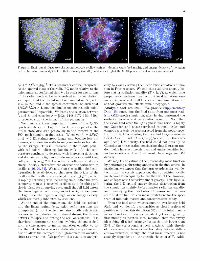
Figure 1. Each panel illustrates the string network (yellow strings), domain walls (red mesh), and energy density of the axionfield (blue-white intensity) before (left), during (middle), and after (right) the QCD phase transition (see animation).

by λ ≡ λf2a/ma(η1)2. This parameter can be interpreted

as the squared mass of the radial PQ mode relative to theaxion mass, at conformal time η1. In order for excitationsof the radial mode to be well-resolved in our simulation,we require that the resolution of our simulation ∆x, withx = a1H1x and x the spatial coordinate, be such that1/(ηλ1/2∆x) > 1, making simulations for realistic axion

parameters λ impossible. We break the relation betweenλ and fa and consider λ = [1024, 1448, 3072, 3584, 5504]in order to study the impact of this parameter.

We illustrate three important phases of the QCD-epoch simulation in Fig. 1. The left-most panel is theinitial state discussed previously in the context of thePQ-epoch simulation final-state. When ma(η) = 3H(η)at η ≈ 1.22, strings grow longer and become less nu-merous, with domain walls forming on surfaces boundedby the strings. This is illustrated in the middle panel,with red colors indicating domain walls. As the tem-perature continues to decrease with increasing η, stringsand domain walls tighten and decrease in size until theycollapse. By η & 2.0, the network collapses in its en-tirety. Shortly thereafter, we observe the formation ofoscillons [16, 20, 54]. We note that the oscillon field con-figuration is relativistic, so that near the origin of theoscillons the oscillation wavelength is ∼ma(η)−1, whichis rapidly shrinking with increasing time. After the zero-temperature mass is reached, oscillons stop shrinking andslowly dissipate at varying rates until the full field entersthe linear regime. White regions in the right-most panelof Fig. 1 denote regions of high axion energy density,which are mostly inhabited by oscillons.

At the end of the simulation, the field has relaxedinto the linear regime (e.g., axion self-interactions areunimportant), but the field remains mildly relativisticbecause axion radiation is produced during the string-network collapse and during the oscillon collapse. It istherefore important to continue evolving the axion fielduntil a time nearer to matter-radiation equality to al-low the field to become non-relativistic everywhere andalso to allow the compact but high-momentum overden-sities to spread out. We perform this evolution analyti-

cally by exactly solving the linear axion equations of mo-tion in Fourier space. We end this evolution shortly be-fore matter-radiation equality (T ∼ keV), at which timeproper velocities have frozen out but local radiation dom-ination is preserved at all locations in our simulation boxso that gravitational effects remain negligible.Analysis and results.— We provide SupplementaryData [55] containing the final state from our most real-istic QCD-epoch simulation, after having performed theevolution to near matter-radiation equality. Note thatthe axion field after the QCD phase transition is highlynon-Gaussian and phase-correlated at small scales andcannot accurately be reconstructed from the power spec-trum. In fact considering that we find large overdensi-ties δ (δ ∼ 10), with δ = (ρ − ρ)/ρ and ρ (ρ) the aver-age (local) DM density, the field could not possibly beGaussian at these scales, considering that Gaussian ran-dom fields have symmetric over and under-densities butunder-densities with δ < −1 would have negative DMdensity.

We may try to estimate the present-day mass functionby performing a clustering analysis on the final states. Inparticular, we expect that the large overdensities will de-tach from the cosmic expansion, due to reaching locallymatter-radiation equality before the rest of the Universe,and collapse onto themselves under gravity. Thus by clus-tering the 3-D spatial energy density distribution fromthe simulation slightly before matter-radiation equalityand quantifying the distribution of masses and overden-sities that we find, we can make predictions for the spec-trum of minihalo masses and concentrations today.

From the final-state we construct an overdensity fieldδ(x), and we identify overdensities as closed regions ofpositive δ. Under this definition 50% of the total mass isin overdensities. In practice, we identify these regions byfirst finding all positive local maxima, then recursivelyidentifying all neighboring grid sites that are larger than20% of the corresponding local maxima. This thresh-old is necessary to have a clear boundary between differ-ent overdensities, though the final mass function is notstrongly dependent on the specific choice of 20%. Addi-

4

tionally, we discard overdensities that consist of less than80 grid sites to avoid discretization issues in the final re-sult. Note that we discard only about 0.8% of the totalmass that would otherwise be assigned to an overdensitydue to the 80 grid-site limit and 20% threshold. We as-sign to each overdensity a mass M and a single meanconcentration parameter δ.

An illustration of our clustering procedure is shownin Fig. 2. In that figure we show a 2-dimensional slice

0.00 0.25 0.50 0.75 1.000.0

0.2

0.4

0.6

0.8

1.0

L[1

/a1H

1]

L [1/a1H1]

η = 7.0

0.25 0.5 0.75 1.0

η = ηMR

−1

0

1

2

3

4

5

6

7

8

δ

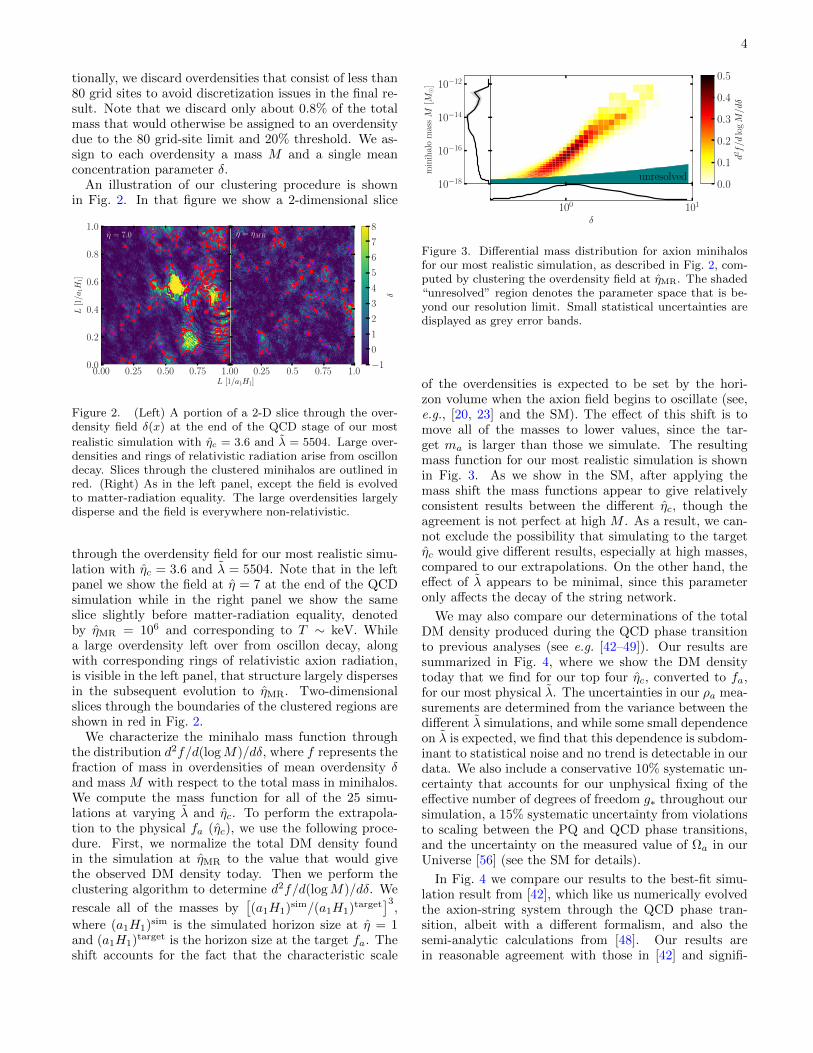
Figure 2. (Left) A portion of a 2-D slice through the over-density field δ(x) at the end of the QCD stage of our most

realistic simulation with ηc = 3.6 and λ = 5504. Large over-densities and rings of relativistic radiation arise from oscillondecay. Slices through the clustered minihalos are outlined inred. (Right) As in the left panel, except the field is evolvedto matter-radiation equality. The large overdensities largelydisperse and the field is everywhere non-relativistic.

through the overdensity field for our most realistic simu-lation with ηc = 3.6 and λ = 5504. Note that in the leftpanel we show the field at η = 7 at the end of the QCDsimulation while in the right panel we show the sameslice slightly before matter-radiation equality, denotedby ηMR = 106 and corresponding to T ∼ keV. Whilea large overdensity left over from oscillon decay, alongwith corresponding rings of relativistic axion radiation,is visible in the left panel, that structure largely dispersesin the subsequent evolution to ηMR. Two-dimensionalslices through the boundaries of the clustered regions areshown in red in Fig. 2.

We characterize the minihalo mass function throughthe distribution d2f/d(logM)/dδ, where f represents thefraction of mass in overdensities of mean overdensity δand mass M with respect to the total mass in minihalos.We compute the mass function for all of the 25 simu-lations at varying λ and ηc. To perform the extrapola-tion to the physical fa (ηc), we use the following proce-dure. First, we normalize the total DM density foundin the simulation at ηMR to the value that would givethe observed DM density today. Then we perform theclustering algorithm to determine d2f/d(logM)/dδ. We

rescale all of the masses by[(a1H1)sim/(a1H1)target

]3,

where (a1H1)sim is the simulated horizon size at η = 1and (a1H1)target is the horizon size at the target fa. Theshift accounts for the fact that the characteristic scale

unresolved0.0

0.1

0.2

0.3

0.4

0.5

d2 f/d

logM/dδ

100 101

δ

10−18

10−16

10−14

10−12

min

ihal

om

assM

[M

]

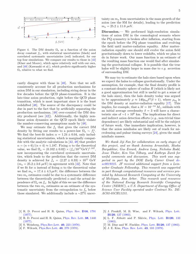
Figure 3. Differential mass distribution for axion minihalosfor our most realistic simulation, as described in Fig. 2, com-puted by clustering the overdensity field at ηMR. The shaded“unresolved” region denotes the parameter space that is be-yond our resolution limit. Small statistical uncertainties aredisplayed as grey error bands.

of the overdensities is expected to be set by the hori-zon volume when the axion field begins to oscillate (see,e.g., [20, 23] and the SM). The effect of this shift is tomove all of the masses to lower values, since the tar-get ma is larger than those we simulate. The resultingmass function for our most realistic simulation is shownin Fig. 3. As we show in the SM, after applying themass shift the mass functions appear to give relativelyconsistent results between the different ηc, though theagreement is not perfect at high M . As a result, we can-not exclude the possibility that simulating to the targetηc would give different results, especially at high masses,compared to our extrapolations. On the other hand, theeffect of λ appears to be minimal, since this parameteronly affects the decay of the string network.

We may also compare our determinations of the totalDM density produced during the QCD phase transitionto previous analyses (see e.g. [42–49]). Our results aresummarized in Fig. 4, where we show the DM densitytoday that we find for our top four ηc, converted to fa,for our most physical λ. The uncertainties in our ρa mea-surements are determined from the variance between thedifferent λ simulations, and while some small dependenceon λ is expected, we find that this dependence is subdom-inant to statistical noise and no trend is detectable in ourdata. We also include a conservative 10% systematic un-certainty that accounts for our unphysical fixing of theeffective number of degrees of freedom g∗ throughout oursimulation, a 15% systematic uncertainty from violationsto scaling between the PQ and QCD phase transitions,and the uncertainty on the measured value of Ωa in ourUniverse [56] (see the SM for details).

In Fig. 4 we compare our results to the best-fit simu-lation result from [42], which like us numerically evolvedthe axion-string system through the QCD phase tran-sition, albeit with a different formalism, and also thesemi-analytic calculations from [48]. Our results arein reasonable agreement with those in [42] and signifi-

5

5× 1014 1015

fa [GeV]

104

Ωa

Klaer and Moore Kawasaki et al. This Work

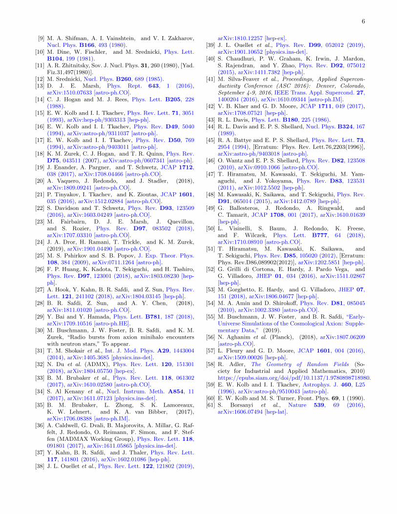
Figure 4. The DM density Ωa as a function of the axiondecay constant fa, with statistical uncertainties (black) andcorrelated systematic uncertainties (red) indicated, for ourtop four simulations. We compare our results to those in [42](Klaer and Moore), which agree relatively well with our own,and [48] (Kawasaki et al.), which predicts significantly higherΩa relative to what we find.

cantly disagree with those in [48]. Note that we self-consistently account for all production mechanisms foraxion DM in our simulation, including string decay in thefew decades before the QCD phase-transition. It is thelate-time axion production, right before the QCD phasetransition, which is most important since it is the leastredshifted [48]. The source of the discrepancy could bedue in part to the fact that by artificially separating theproduction mechanisms, [48] over-counted the DM den-sity produced (see [42]). Additionally, the highly non-linear axion dynamics at the QCD epoch likely violatethe number-conserving assumptions made by [48].

We may estimate the fa that gives the correct DMdensity by fitting our results to a power-law Ωa ∼ fαa .We find the best-fit index α = 1.24 ± 0.04, only includ-ing statistical uncertainties, which is marginally compat-ible with the analytic calculations in [42, 48] that predictα = (n+ 6)/(n+ 4) ≈ 1.187. Fixing α to the theoreticalvalue, we find Ωa = (0.102 ± 0.02) × (fa/1011GeV)1.187,now incorporating the correlated systematic uncertain-ties, which leads to the prediction that the correct DMdensity is achieved for fa = (2.27 ± 0.33) × 1011 GeV(ma = 25.2±3.6 µeV) in agreement with [42]. Note thatif we fit for α instead of fixing α to the theoretical valuewe find ma = 17.4± 4.5µeV; the difference between thetwo ma estimates could be due to a systematic differencebetween the theoretically predicted α and the actual de-pendence of Ωa on fa. In light of this we use the differencebetween the two ma estimates as an estimate of the sys-tematic uncertainty from the extrapolation to fa belowthose simulated. We additionally include a ∼27% uncer-

tainty on ma from uncertainties in the mass growth of theaxion (see the SM for details), leading to the predictionma = 25.2± 11.0 µeV.

Discussion.— We performed high-resolution simula-tions of axion DM in the cosmological scenario wherethe PQ symmetry is broken after inflation, starting fromthe epoch before the PQ phase transition and evolvingthe field until matter-radiation equality. After matter-radiation equality one should still evolve the axion fieldgravitationally down to lower redshifts, which we plan todo in future work. Our mass function is an estimate ofthe resulting mass function one would find after simulat-ing the gravitational collapse. It is possible that the truehalos will be slightly larger in mass due to e.g. accretionof surrounding DM.

We may try to estimate the halo sizes based upon whenwe expect the halos to collapse gravitationally. Under theassumption, for example, that the final density profile isa constant-density sphere of radius R (which is likely nota good approximation but still is useful to get a sense ofthe halo sizes), then the halo density today was arguedto be approximately ρ ≈ 140ρeqδ

3(δ + 1), where ρeq isthe DM density at matter-radiation equality [17]. Thisimplies, for example, that a M = 10−14 M subhalo withan initial average overdensity δ = 3 will have a charac-teristic size of ∼1× 106 km. The implications for directand indirect axion detection efforts (e.g., non-trivial timedependence) are likely substantial and will be the subjectof future work. One immediate implication, however, isthat the axion minihalos are likely out of reach for mi-crolensing and pulsar timing surveys [24], given the smallminihalo masses.

We thank Jiji Fan for collaboration on early stages ofthis project, and we thank Asimina Arvanitaki, MashaBaryakhtar, Gus Evrard, Andrew Long, Nicholas Rodd,Jesse Thaler, Ken Van Tilburg, and Kathryn Zurek foruseful comments and discussion. This work was sup-ported in part by the DOE Early Career Grant de-sc0019225. JF received additional support from a Lein-weber Graduate Fellowship. This research was supportedin part through computational resources and services pro-vided by Advanced Research Computing at the Universityof Michigan, Ann Arbor. This research used resourcesof the National Energy Research Scientific ComputingCenter (NERSC), a U.S. Department of Energy Office ofScience User Facility operated under Contract No. DE-AC02-05CH11231.

[1] R. D. Peccei and H. R. Quinn, Phys. Rev. D16, 1791(1977).

[2] R. D. Peccei and H. R. Quinn, Phys. Rev. Lett. 38, 1440(1977).

[3] S. Weinberg, Phys.Rev.Lett. 40, 223 (1978).[4] F. Wilczek, Phys.Rev.Lett. 40, 279 (1978).

[5] J. Preskill, M. B. Wise, and F. Wilczek, Phys. Lett.B120, 127 (1983).

[6] L. F. Abbott and P. Sikivie, Phys. Lett. B120, 133(1983).

[7] M. Dine and W. Fischler, Phys. Lett. B120, 137 (1983).[8] J. E. Kim, Phys. Rev. Lett. 43, 103 (1979).

6

[9] M. A. Shifman, A. I. Vainshtein, and V. I. Zakharov,Nucl. Phys. B166, 493 (1980).

[10] M. Dine, W. Fischler, and M. Srednicki, Phys. Lett.B104, 199 (1981).

[11] A. R. Zhitnitsky, Sov. J. Nucl. Phys. 31, 260 (1980), [Yad.Fiz.31,497(1980)].

[12] M. Srednicki, Nucl. Phys. B260, 689 (1985).[13] D. J. E. Marsh, Phys. Rept. 643, 1 (2016),

arXiv:1510.07633 [astro-ph.CO].[14] C. J. Hogan and M. J. Rees, Phys. Lett. B205, 228

(1988).[15] E. W. Kolb and I. I. Tkachev, Phys. Rev. Lett. 71, 3051

(1993), arXiv:hep-ph/9303313 [hep-ph].[16] E. W. Kolb and I. I. Tkachev, Phys. Rev. D49, 5040

(1994), arXiv:astro-ph/9311037 [astro-ph].[17] E. W. Kolb and I. I. Tkachev, Phys. Rev. D50, 769

(1994), arXiv:astro-ph/9403011 [astro-ph].[18] K. M. Zurek, C. J. Hogan, and T. R. Quinn, Phys. Rev.

D75, 043511 (2007), arXiv:astro-ph/0607341 [astro-ph].[19] J. Enander, A. Pargner, and T. Schwetz, JCAP 1712,

038 (2017), arXiv:1708.04466 [astro-ph.CO].[20] A. Vaquero, J. Redondo, and J. Stadler, (2018),

arXiv:1809.09241 [astro-ph.CO].[21] P. Tinyakov, I. Tkachev, and K. Zioutas, JCAP 1601,

035 (2016), arXiv:1512.02884 [astro-ph.CO].[22] S. Davidson and T. Schwetz, Phys. Rev. D93, 123509

(2016), arXiv:1603.04249 [astro-ph.CO].[23] M. Fairbairn, D. J. E. Marsh, J. Quevillon,

and S. Rozier, Phys. Rev. D97, 083502 (2018),arXiv:1707.03310 [astro-ph.CO].

[24] J. A. Dror, H. Ramani, T. Trickle, and K. M. Zurek,(2019), arXiv:1901.04490 [astro-ph.CO].

[25] M. S. Pshirkov and S. B. Popov, J. Exp. Theor. Phys.108, 384 (2009), arXiv:0711.1264 [astro-ph].

[26] F. P. Huang, K. Kadota, T. Sekiguchi, and H. Tashiro,Phys. Rev. D97, 123001 (2018), arXiv:1803.08230 [hep-ph].

[27] A. Hook, Y. Kahn, B. R. Safdi, and Z. Sun, Phys. Rev.Lett. 121, 241102 (2018), arXiv:1804.03145 [hep-ph].

[28] B. R. Safdi, Z. Sun, and A. Y. Chen, (2018),arXiv:1811.01020 [astro-ph.CO].

[29] Y. Bai and Y. Hamada, Phys. Lett. B781, 187 (2018),arXiv:1709.10516 [astro-ph.HE].

[30] M. Buschmann, J. W. Foster, B. R. Safdi, and K. M.Zurek, “Radio bursts from axion minihalo encounterswith neutron stars,” To appear.

[31] T. M. Shokair et al., Int. J. Mod. Phys. A29, 1443004(2014), arXiv:1405.3685 [physics.ins-det].

[32] N. Du et al. (ADMX), Phys. Rev. Lett. 120, 151301(2018), arXiv:1804.05750 [hep-ex].

[33] B. M. Brubaker et al., Phys. Rev. Lett. 118, 061302(2017), arXiv:1610.02580 [astro-ph.CO].

[34] S. Al Kenany et al., Nucl. Instrum. Meth. A854, 11(2017), arXiv:1611.07123 [physics.ins-det].

[35] B. M. Brubaker, L. Zhong, S. K. Lamoreaux,K. W. Lehnert, and K. A. van Bibber, (2017),arXiv:1706.08388 [astro-ph.IM].

[36] A. Caldwell, G. Dvali, B. Majorovits, A. Millar, G. Raf-felt, J. Redondo, O. Reimann, F. Simon, and F. Stef-fen (MADMAX Working Group), Phys. Rev. Lett. 118,091801 (2017), arXiv:1611.05865 [physics.ins-det].

[37] Y. Kahn, B. R. Safdi, and J. Thaler, Phys. Rev. Lett.117, 141801 (2016), arXiv:1602.01086 [hep-ph].

[38] J. L. Ouellet et al., Phys. Rev. Lett. 122, 121802 (2019),

arXiv:1810.12257 [hep-ex].[39] J. L. Ouellet et al., Phys. Rev. D99, 052012 (2019),

arXiv:1901.10652 [physics.ins-det].[40] S. Chaudhuri, P. W. Graham, K. Irwin, J. Mardon,

S. Rajendran, and Y. Zhao, Phys. Rev. D92, 075012(2015), arXiv:1411.7382 [hep-ph].

[41] M. Silva-Feaver et al., Proceedings, Applied Supercon-ductivity Conference (ASC 2016): Denver, Colorado,September 4-9, 2016, IEEE Trans. Appl. Supercond. 27,1400204 (2016), arXiv:1610.09344 [astro-ph.IM].

[42] V. B. Klaer and G. D. Moore, JCAP 1711, 049 (2017),arXiv:1708.07521 [hep-ph].

[43] R. L. Davis, Phys. Lett. B180, 225 (1986).[44] R. L. Davis and E. P. S. Shellard, Nucl. Phys. B324, 167

(1989).[45] R. A. Battye and E. P. S. Shellard, Phys. Rev. Lett. 73,

2954 (1994), [Erratum: Phys. Rev. Lett.76,2203(1996)],arXiv:astro-ph/9403018 [astro-ph].

[46] O. Wantz and E. P. S. Shellard, Phys. Rev. D82, 123508(2010), arXiv:0910.1066 [astro-ph.CO].

[47] T. Hiramatsu, M. Kawasaki, T. Sekiguchi, M. Yam-aguchi, and J. Yokoyama, Phys. Rev. D83, 123531(2011), arXiv:1012.5502 [hep-ph].

[48] M. Kawasaki, K. Saikawa, and T. Sekiguchi, Phys. Rev.D91, 065014 (2015), arXiv:1412.0789 [hep-ph].

[49] G. Ballesteros, J. Redondo, A. Ringwald, andC. Tamarit, JCAP 1708, 001 (2017), arXiv:1610.01639[hep-ph].

[50] L. Visinelli, S. Baum, J. Redondo, K. Freese,and F. Wilczek, Phys. Lett. B777, 64 (2018),arXiv:1710.08910 [astro-ph.CO].

[51] T. Hiramatsu, M. Kawasaki, K. Saikawa, andT. Sekiguchi, Phys. Rev. D85, 105020 (2012), [Erratum:Phys. Rev.D86,089902(2012)], arXiv:1202.5851 [hep-ph].

[52] G. Grilli di Cortona, E. Hardy, J. Pardo Vega, andG. Villadoro, JHEP 01, 034 (2016), arXiv:1511.02867[hep-ph].

[53] M. Gorghetto, E. Hardy, and G. Villadoro, JHEP 07,151 (2018), arXiv:1806.04677 [hep-ph].

[54] M. A. Amin and D. Shirokoff, Phys. Rev. D81, 085045(2010), arXiv:1002.3380 [astro-ph.CO].

[55] M. Buschmann, J. W. Foster, and B. R. Safdi, “Early-Universe Simulations of the Cosmological Axion: Supple-mentary Data,” (2019).

[56] N. Aghanim et al. (Planck), (2018), arXiv:1807.06209[astro-ph.CO].

[57] L. Fleury and G. D. Moore, JCAP 1601, 004 (2016),arXiv:1509.00026 [hep-ph].

[58] R. Adler, The Geometry of Random Fields (So-ciety for Industrial and Applied Mathematics, 2010)https://epubs.siam.org/doi/pdf/10.1137/1.9780898718980.

[59] E. W. Kolb and I. I. Tkachev, Astrophys. J. 460, L25(1996), arXiv:astro-ph/9510043 [astro-ph].

[60] E. W. Kolb and M. S. Turner, Front. Phys. 69, 1 (1990).[61] S. Borsanyi et al., Nature 539, 69 (2016),

arXiv:1606.07494 [hep-lat].

1

Supplementary Material for Early-Universe Simulations of the Cosmological Axion

Malte Buschmann, Joshua W. Foster, and Benjamin R. Safdi

Leinweber Center for Theoretical Physics, Department of Physics, University of Michigan, Ann Arbor, MI 48109

This Supplementary Material contains additional results and explanations of our methods that clarify and supportthe results presented in the main Letter. We begin with a detailed explanation of the equations of motion andinitial conditions used in our simulations. Next, we present extended results for the overdensity spectrum and DMdensity. We then present a modified simulation that allows us to quantify the systematic uncertainty in the DMdensity determination by assuming a fixed number of relativistic degrees of freedom. Additionally, we quantify theuncertainty on the DM density induced by uncertainties in the mass growth of the axion, and finally we consider theeffects of violations to the scaling solution on our final results.

I. SIMULATION EQUATIONS OF MOTION

Our phenomenological Lagrangian describing the PQ field is adopted from the construction of [51] and is of theform

LPQ =1

2|∂Φ|2 − λ

4

(|Φ|2 − f2

a

)2 − λT 2

6|Φ|2 −ma(T )2f2

a [1− cos Arg(Φ)], (S1)

where Φ is the complex PQ scalar, T is the temperature, λ is the PQ quartic coupling strength, fa is the PQ-scaleidentified as the axion decay constant, and ma(T ) is the temperature-dependent axion mass [51]. The parametrizationof the temperature-dependent mass is adopted from the leading order term in the fit in [46]. Explicitly, the axionmass is parametrized by

ma(T )2 = min

[αaΛ4

f2a (T/Λ)n

, ma

], (S2)

for α = 1.68 × 10−7, Λ = 400 MeV and n = 6.68. The growth of the mass is truncated at T ≈ 100 MeV. Thezero-temperature mass is given by

m2a =

m2πf

2π

f2a

mumd

(mu +md)2, (S3)

where mπ is the pion mass, fπ is the pion decay constant, mu/d is the up/down quark mass. Details of the temperature-dependent axion mass, or equivalently, the topological susceptibility, remain uncertain, especially at low temperatures.Note that we do not explore here how our results are affected by uncertainties in the temperature-dependent axionmass, though doing so is a worthwhile direction for future work.

Decomposing the complex scalar as Φ = φ1 + iφ2, and assuming a radiation-dominated cosmological background,leads to equations of motion in metric coordinates of the form

φ1 + 3Hφ1 −1

R2∇2φ1 +

1

3λφ1

[3(φ2

1 + φ22 − f2

a

)+ T 2

]− ma(T )2φ2

2

(φ21 + φ2

2) 3/2= 0 (S4)

φ2 + 3Hφ2 −1

R2∇2φ2 +

1

3λφ2

[3(φ2

1 + φ22 − f2

a

)+ T 2

]+ma(T )2φ1φ2

(φ21 + φ2

2)3/2

= 0 . (S5)

Over temperatures T & 100 MeV, the number of relativistic degrees of freedom g∗ in the Standard Model is expectedto vary only mildly. For simplicity, we therefore assume g∗ = 81, which is a typical value adopted at high temperatures(though later in the SM we explore the systematic uncertainty introduced by this assumption). It is useful to definea dimensionless conformal time η such that

η =R

R(T = T1)=

R

R1=

(t

t1

)1/2

, (S6)

where R is the scale factor and the time t1 (with T (t1) ≡ T1) is a reference time that will be defined differently in thePQ and QCD epoch simulations.

The axion-mass term is not included in our PQ-epoch simulations. In our QCD-epoch simulations, on the otherhand, the mass term is included and drives the dynamics. In this case, the mass grows until the cutoff temperature

2

Tc at which point the axion mass reaches its zero-temperature value; the corresponding conformal time is given byηc = R(T = Tc)/R1. Rewriting (S5) with the dimensionless coordinates, we then find

ψ′′1 +2

ηψ′1 − ∇2ψ1 +

1

H21

[λψ1

(η2f2

a

(ψ2

1 + ψ22 − 1

)+

1

3T 2

1

)−m2

a(T1)η2min(η, ηc)n

(ψ2

2

(ψ21 + ψ2

2) 3/2

)]= 0 (S7)

ψ′′2 +2

ηψ′2 − ∇2ψ2 +

1

H21

[λψ2

(η2f2

a

(ψ2

1 + ψ22 − 1

)+

1

3T 2

1

)+m2

a(T1)η2min(η, ηc)n

(ψ1ψ2

(ψ21 + ψ2

2)3/2

)]= 0 , (S8)

where φ = faψ, primes denote derivatives with respect to η, and the spatial gradient is taken with respect tox = a1H1x.

A. The PQ Epoch

Simulations in the PQ epoch occur at T ΛQCD and so the temperature-dependent axion mass may be neglected.We therefore take our equations of motion to be

ψ′′1 +2

ηψ′1 − ∇2ψ1 + λψ1

[η2(ψ2

1 + ψ22 − 1

)+

T 21

3f2a

]= 0 (S9)

ψ′′2 +2

ηψ′2 − ∇2ψ2 + λψ2

[η2(ψ2

1 + ψ22 − 1

)+

T 21

3f2a

]= 0 , (S10)

and we fix η = 1 to be the time at which H1 = fa. Note that for our PQ-epoch simulations we refer to η, definedin (S6), as η in order to avoid confusion with the dimensionless conformal time η used in the QCD-epoch simulations.The ratio (T1/fa)2 is determined by (

T1

fa

)2

≈ 8.4× 105

(1012 GeV

fa

). (S11)

In principle, it would seem that axions of different decay constants would require different simulations in the PQepoch. However, this ratio is degenerate with our choice of physical box size and dynamical range in η in a particularsimulation, allowing us to perform only one PQ simulation and interpret its output as the initial state of the axionfield for several different values of fa. The key assumption behind this, however, is that at late times after the PQphase transition the field enters the scaling regime so that we may reinterpret the output of the PQ simulation inthe appropriately rescaled box as the initial state of the QCD simulation at much lower temperatures. Note that thevalue of λ is a free parameter, which we naturally choose to be λ = 1 though it has little effect.

1. Initial Conditions for a PQ Scalar

We generate initial conditions for our PQ scalar by taking it to be described by a thermal distribution characterizedby the temperature T at the initial early time. As can be read off from the Lagrangian, each of the two fields has aneffective mass of the form

m2eff = λ

(T 2

3− f2

a

). (S12)

Correlation functions of the initially-free massive scalar fields are given by

〈φi(x)φj(y)〉 = δij

∫dk

2π

nkωkeik · (x−y) (S13)

〈φi(x)φj(y)〉 = δij

∫dk

2πnkωke

ik · (x−y) (S14)

〈φi(x)φj(y)〉 = 0 , (S15)

where overdots denote differentiation with respect to time, and we have defined

nk =1

eωk/T − 1, ωk =

√k2 +m2

eff . (S16)

3

In momentum space, these correlation functions take the form

〈φi(k)φj(k′)〉 =

2πnkωk

δ(k + k′)δij (S17)

〈φi(k)φj(k′)〉 = 2πnkωkδ(k + k′)δij (S18)

〈φi(k)φj(k′)〉 = 0 . (S19)

Our simulations occur on a discrete lattice of finite size, so the correlation functions above lead to initial conditionsset by a realization of a Gaussian random field specified in Fourier space by

〈φi(k)〉 = 0, 〈|φi(k)|2〉 =nkωkL, (S20)

〈φi(k)〉 = 0, 〈|φi(k)|2〉 = nkωkL . (S21)

Note that we include the 50 lowest k-modes in each of the three directions when constructing the initial conditions,and we have verified that including more modes does not affect our results.

B. Early Times in the QCD Epoch

During the QCD epoch, T ∼ ΛQCD, and so the axion mass is non-negligible. Here, we define η = 1 to be the timeat which H1 = ma(T1), with the axion field beginning to oscillate shortly thereafter when ma = 3H. The equationsof motion are then given by

ψ′′1 +2

ηψ′1 − ∇2ψ1 + λη2ψ1(ψ2

1 + ψ22 − 1)−min(η, ηc)

nη2

(ψ2

2

(ψ21 + ψ2

2)3/2

)= 0 (S22)

ψ′′2 +2

ηψ′2 − ∇2ψ2 + λη2ψ2(ψ2

1 + ψ22 − 1) + min(η, ηc)

nη2

(ψ1ψ2

(ψ21 + ψ2

2)3/2

)= 0 , (S23)

where we have neglected the T1 contribution to the PQ scalar mass as it is small compared to fa. The parameter λis defined by

λ = λ

(fa

ma(T1)

)2

(S24)

and can be interpreted as the squared mass of the radial mode |Φ/fa|. For physical parameters we expect λ 1,

though in practice we find that the final results are relatively independent of λ for moderately sized values of theparameter, as described in the main text and later in the SM. Indeed, our choices for λ allow us to resolve the radialmode mass by more than a few grid-spacings, satisfying the requirement of [53] to accurately study the axion spectrum

from string radiation, unlike [20]. There exist additional criteria on the largeness of λ such that the metastability

of topological defects is preserved despite the unphysical smallness of simulated λ in comparison with the rapidlyincreasing axion mass. At all times prior to expected defect collapse, our choices of λ satisfy the simplest constructionof these conditions [20], with our choice of λ = 5504 satisfying the most stringent criteria established in [57]. We note

that we are largely unable to differentiate between simulations at any two particular values of λ, and that our choiceof values appear to have minimal impact, as illustrated further below.

C. Late Times in the QCD Epoch

The presence of topological defects in the axion field at early times during the QCD epoch requires that we fullysimulate both degrees of freedom of the PQ field. Once the topological defects have collapsed, however, we are freeto use the axion-only equations of motion. Our axion is defined by a = faarctan2(φ1, φ2) and has the Lagrangian

L =1

2(∂a)2 −m2

a(T )f2a

[1− cos

(a

fa

)], (S25)

along with corresponding equations of motion

θ′′ +2

ηθ′ − ∇2θ + min(η, ηc)

nη2 sin θ = 0 . (S26)

4

Above, we define θ = a/fa. Evolving these equations of motion is formally equivalent to freezing out excitations of

the radial mode by taking λ→∞, which more accurately recovers the true physics of the evolution of the axion fieldfor realistic values of fa. Note that the coordinate x and η here are identical to those used in evolving the two degreesof freedom of the complex scalar performed prior to defect collapse.

D. Analytically Evolving in the Fixed-Mass Small-Field Limit

At late times when the axion mass has reached its zero-temperature value and the axion field has redshiftedconsiderably so that |θ| 1, the equations of motion are linear and well-approximated by

θ′′ +2

ηθ′ −∇2θ + ηnc η

2θ = 0. (S27)

We may solve this equation analytically by going to Fourier space and adopting an ansatz for the solution as

θ(η) = f(η) exp(ik ·x) . (S28)

This ansatz leads to the equation

f ′′(η) +2f ′(η)

η+ f(η)

(η2ηnc + k2

)= 0 , (S29)

which has the general solution

f(η) =exp(− i

2 η2ηn/2c )

η

[C1H− 1

2 η−n/2c

(ηn/2c +ik2

) ( 4√−1ηηn/4c

)+ C2 1F1

(1

4η−n/2c

(ηn/2c + ik2

);

1

2; iη2ηn/2c

)], (S30)

for coefficients C1 and C2 determined by boundary conditions, and where Hn and 1F1 are the analytic continuations ofthe Hermite polynomials and the confluent hypergeometric function of the first kind, respectively. From this analyticsolution, we can transfer late-time field configurations from our simulation to arbitrary large η. Differentiation withrespect to η may be straightforwardly performed to find f ′(η) at large η as well. The computation of the analyticallycontinued Hermite polynomials and hypergeometric functions was performed with the python package mpmath.

We directly compare the differential mass spectrum at η = 7 with the same field analytically evolved to η = ηMR

in Fig. S1. While the basic differential shape is the same, the η = 7 results have a much wider distribution in δ. Inparticular, all overdensities above δ > 10 have vanished by the time matter-radiation equality is reached. However,the peak of the distribution is still around δ = 1. Evolving the fields down to matter-radiation equality is importantbecause many of the modes are generated with high momentum at the QCD epoch, causing the large overdensitiesto disperse by the time of matter-radiation equality.

II. STUDYING THE (OVER)DENSITY FIELD

Our interest in this work is studying the energy density field ρ and the overdensity field δ = (ρ − ρ)/ρ realizedin the axion field from our simulations. The axion energy density for the axion field a = faθ is computed by theHamiltonian density

H = f2a

[1

2θ2 +

1

2R2(∇θ)2 +m2

a(1− cos θ)

], (S31)

which can be rewritten in simulation units as

H = m2af

2a

[θ′2 + (∇θ)2

2η6.68c η2

+ (1− cos θ)

], (S32)

assuming η > ηc. At late times, the Hamiltonian is approximately

H ≈ m2af

2a

2

(θ′2

ηnc η2

+ θ2

), (S33)

when all modes in the simulation are non-relativistic and the field values are small.

5

10−1 100 101 102

δ

10−18

10−16

10−14

10−12m

inih

alo

mas

sM

[M

]

unresolved

η = 7

0.00

0.02

0.04

0.06

0.08

0.10

0.12

0.14

d2 f/d

logM/dδ

10−17 10−16 10−15 10−14 10−13 10−12

M [M]

0.0

0.1

0.2

0.3

0.4

0.5

df/d

logM

η = 7

η = ηMR

10−1 100 101 102

δ

10−18

10−16

10−14

10−12

min

ihal

om

assM

[M

]

unresolved

η = ηMR

0.00

0.05

0.10

0.15

0.20

0.25

0.30

0.35

0.40

d2 f/d

logM/dδ

10−1 100 101 102

δ

10−4

10−3

10−2

10−1

df/dδ

η = 7

η = ηMR

Figure S1. Double differential mass fractions for axion minihalos as a function of the concentration parameter δ and mass M .In the top left we compute that mass function using the field immediately after the QCD phase transition, at η = 7, while inthe bottom left we use the more correct procedure of first evolving to η = ηMR before performing the clustering procedure.Evolving to matter-radiation equality gives the most over-dense regions time to expand and results in less dense overdensities,as compared to the incorrect procedure shown in the top left. This is perhaps even more apparent in the single differentialmass fractions as a function of the mass M (top right) and concentration parameter δ (bottom right). These results are based

on our most realistic simulation with ηc = 3.6 and λ = 5504. Error bars are statistical, and we do not extend the df/d logMcurves to lower masses as we are unable to resolve those properly.

A. Oscillons

Large overdensities right after the QCD phase transition are caused by oscillons. Oscillons are, in contrast tostrings and domain walls, not topological defects but arise due to non-linearities in the equation of motions, formingat locations where the the axion self-interaction dominates the Hubble friction. As a result, the first oscillons format the location of collapsed strings and domain walls, where the axion remains excited and reaches large field values.However, at later times, oscillons are observed forming throughout the simulation box. The dynamics of the oscillonsare highly non-trivial, especially as the axion self-interaction increases in strength with the growing axion mass.

Oscillons decrease in size over time following the oscillation wavelength ∼ma(T )−1, as axions in the core arerelativistic. Good spatial resolution is therefore needed to resolve them. In order to study their behavior we performa 2D (two spatial dimensions, one time) simulation using the same simulation setup in the PQ- and QCD-epoch asin 3D. We find that there is no qualitative difference between 2D and 3D simulations regarding oscillons, but goingto 2D allows us to increase the spatial resolution to 40962 grid sites and to subsequently increase ηc.

We illustrate the evolution of an oscillon in Fig. S2. Two scenarios are considered with different truncation points ofthe mass growth, ηc = 4.0 and ηc = 6.0. Note how the radius of the oscillon decreases as long as ma(T ) is increasing.The circles in S2 have radius ma(T )−1, and the oscillon cores are seen to track this scale. Subsequently, if the massgrowth is truncated at ηc = 4.0, the radius of the oscillon is constant as well. When the mass growth is cut-off, thedensity contrast at the core of the oscillon slowly decreases over time and the oscillons dissipate, as can be seen inthe two lower right panels in Fig. S2.

B. Calculating the Axion Relic Abundance

To calculate the axion DM abundance as a function of ma, we first need to understand the relationship between themass cutoff conformal time ηc and the decay constant fa. Here we use the relation T1/ηc = Tc, with Tc ≈ 100 MeV.

6

η = 3.0 η = 3.5 η = 4.0

η = 5.0 η = 6.0

η = 5.0 η = 6.0

ma(T ) keeps growing

ma(T ) constant

Figure S2. Illustration of an oscillon (log(ρ/ρ)) at different times in a 2D simulation. Two scenarios are considered with differenttruncation points of the mass growth, ηc = 4.0 and ηc = 6.0. The three left panels are identical in both scenarios, while thetwo top right panels are for ηc = 6.0, and the two bottom panels are for ηc = 4.0. The radius of the oscillon is proportionalto the oscillation frequency ∼ ma(T )−1 (circles of that radius are shown in dashed blue) and as such is decreasing over time.The oscillon central density slowly dissipates after the mass growth ends, as seen in the bottom right panels for ηc = 4.0.

This allows us to solve for fa in terms of ηc. The energy densities are calculated from the axion field and its derivativesaccording to (S33) after numerically evolving until η = 7, then analytically evolving until ηMR = 106, at which pointthe contribution of the gradient term to the energy density is negligible. As a side note, our definition of ηMR actuallyputs us at slightly earlier times than global matter-radiation equality. This us because matter-radiation equality is,locally, reached earlier for the largest overdensities and because we want to make sure that gravitational interactionscan be neglected. In particular, note that the temperature corresponding to ηMR is given by TMR = Tcηc/ηMR. Forour most realistic simulation with ηc = 3.6 this corresponds to TMR ≈ 0.5 keV. However, if we reinterpret the finalstate for a more realistic axion with ma ≈ 25 µeV, which has a higher ηc, then TMR ≈ 4 keV. In practice, though, theexact value of TMR is not important because by these temperatures the proper motions in the axion field are frozenout and the field is thus not evolving non trivially. As a consequence our results (both for the DM density and forthe spectrum of overdensities) are not sensitive to small (or even relatively large) changes to the exact value of η thatwe evolve to.

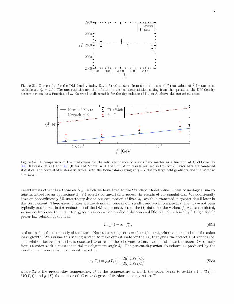
Note that we present our results in terms of the DM density fraction today Ωa, which is defined as the ratio ofthe average energy density today in DM relative to the observed critical energy density. We compute statistical errorbars at each value of fa from the variance as a function of λ at fixed ηc. We note that no trend is visible in the datafor the dependence of Ωa on λ, as is shown in Fig. S3. The statistical noise is inferred from the spread in Ωa values,which are determined from the output at ηMR, between different λ. The observed variations are consistent with theexpected noise from Poisson counting statistics due to having a finite number of overdensities within the simulationbox.

In Fig. S4 we show our results for Ωa as a function of fa, compared to earlier predictions in [48] and [42]. Forreference, we also include predictions for the relic abundance based on the field value and the time derivative at η = 7.Here it is less straightforward to determine the DM axion abundance, relative to taking the results at ηMR, as some ofthe modes in the simulation are still relativistic. This introduces an additional systematic uncertainty, since the fieldis not completely red-shifting like radiation at this time. For these reasons it is important to evolve the field until itis completely non-relativistic before measuring the DM density.

Because the ratio of the axion mass density to entropy density is constant after the axions have become non-relativistic and the number of axions is conserved, we can redshift our energy density from our matter-radiationequality ηMR to today. Then, we compare this energy density to the most up-to-date measurement of the averageDM density in the Universe today ρDM = 33.5 ± 0.6 M/kpc3 [56]. Note that we have propagated all cosmological

7

1000 2000 3000 4000 5000

λ

2000

2200

2400

2600

2800

Ωa

Average

Data

Figure S3. Our results for the DM density today Ωa, inferred at ηMR, from simulations at different values of λ for our mostrealistic ηc: ηc = 3.6. The uncertainties are the inferred statistical uncertainties arising from the spread in the DM densitydeterminations as a function of λ. No trend is discernible for the dependence of Ωa on λ, above the statistical noise.

5× 1014 1015

fa [GeV]

104

Ωa

Klaer and Moore

Kawasaki et al.

This Work

η = 7

Figure S4. A comparison of the predictions for the relic abundance of axions dark matter as a function of fa obtained in[48] (Kawasaki et al.) and [42] (Klaer and Moore) with the simulation results realized in this work. Error bars are combinedstatistical and correlated systematic errors, with the former dominating at η = 7 due to large field gradients and the latter atη = ηMR.

uncertainties other than those on Neff , which we have fixed to the Standard Model value. These cosmological uncer-tainties introduce an approximately 3% correlated uncertainty across the results of our simulations. We additionallyhave an approximately 8% uncertainty due to our assumption of fixed g∗, which is examined in greater detail later inthis Supplement. These uncertainties are the dominant ones in our results, and we emphasize that they have not beentypically considered in determinations of the DM axion mass. From the Ωa data, for the various fa values simulated,we may extrapolate to predict the fa for an axion which produces the observed DM relic abundance by fitting a simplepower law relation of the form

Ωa(fa) = c1 · fαa , (S34)

as discussed in the main body of this work. Note that we expect α = (6+n)/(4+n), where n is the index of the axionmass growth. We assume this scaling is valid to make our estimate for the ma that gives the correct DM abundance.The relation between α and n is expected to arise for the following reason. Let us estimate the axion DM densityfrom an axion with a constant initial misalignment angle θi. The present-day axion abundance as produced by themisalignment mechanism can be estimated by

ρa(T0) = ρa(T3)ma(T0)

ma(T3)

g∗(T0)T 30

g∗(T1)T 33

, (S35)

where T0 is the present-day temperature, T3 is the temperature at which the axion began to oscillate (ma(T3) =3H(T3)), and g∗(T ) the number of effective degrees of freedom at temperature T .

8

The initial axion abundance ρa(T1) is given

ρa(T1) =ma(T1)2f2

a

2θ2i , (S36)

Anharmonicity factors can be included, but have no temperature or fa dependence. The temperature T3 depends on

fa through the relation T3 ∝ f−2/(4+n)a . Substituting these relations in and keeping only terms which depend on fa,

we have

ρa(T0) ∝ f (6+n)/(4+n)a

g∗(T0)

g∗(T3). (S37)

We thus expect the relic abundance to scale with fa like ρa ∝ f (6+n)/(4+n)a . Note that the DM abundance from string

and domain wall production is calculated similarly in [48], and although our results are not consistent with thosepresented in that work, the abundance calculation they present proceeds similarly, yielding string and domain wall

production that scale like f(6+n)/(4+n)a as well.

On the other hand, we may also calculate the the ma that gives the correct DM abundance by using our fit valuefor α, as defined in (S34), instead of the theoretical value. Doing so leads to a slightly lower ma estimate, as describedin the main text.

C. Tests of the Overdensity Field Gaussianity

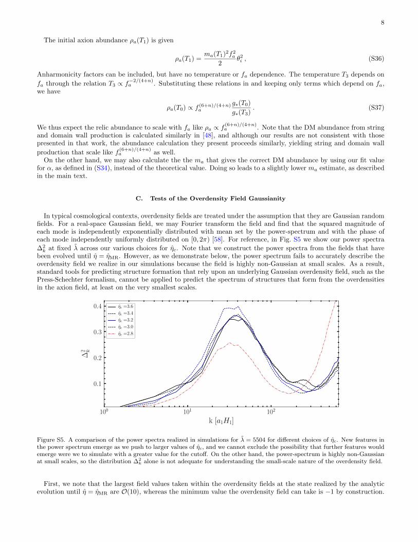
In typical cosmological contexts, overdensity fields are treated under the assumption that they are Gaussian randomfields. For a real-space Gaussian field, we may Fourier transform the field and find that the squared magnitude ofeach mode is independently exponentially distributed with mean set by the power-spectrum and with the phase ofeach mode independently uniformly distributed on [0, 2π) [58]. For reference, in Fig. S5 we show our power spectra

∆2k at fixed λ across our various choices for ηc. Note that we construct the power spectra from the fields that have

been evolved until η = ηMR. However, as we demonstrate below, the power spectrum fails to accurately describe theoverdensity field we realize in our simulations because the field is highly non-Gaussian at small scales. As a result,standard tools for predicting structure formation that rely upon an underlying Gaussian overdensity field, such as thePress-Schechter formalism, cannot be applied to predict the spectrum of structures that form from the overdensitiesin the axion field, at least on the very smallest scales.

100 101 102

k [a1H1]

0.1

0.2

0.3

0.4

∆2 k

ηc =3.6

ηc =3.4

ηc =3.2

ηc =3.0

ηc =2.8

Figure S5. A comparison of the power spectra realized in simulations for λ = 5504 for different choices of ηc. New features inthe power spectrum emerge as we push to larger values of ηc, and we cannot exclude the possibility that further features wouldemerge were we to simulate with a greater value for the cutoff. On the other hand, the power-spectrum is highly non-Gaussianat small scales, so the distribution ∆2

k alone is not adequate for understanding the small-scale nature of the overdensity field.

First, we note that the largest field values taken within the overdensity fields at the state realized by the analyticevolution until η = ηMR are O(10), whereas the minimum value the overdensity field can take is −1 by construction.

9

This is trivially incompatible with the interpretation of the overdensity field as a Gaussian random field, which wouldhave symmetric variance about its mean of 0. For our overdensity fields to realize O(10) maxima with −1 as aconstruction-imposed minimum, there must exist considerable phase-correlations between Fourier modes, contrary tothe uncorrelated phases of a Gaussian random field.

We also may inspect the distribution of power at each mode in the Fourier transformed overdensity field. Ifthe overdensity field were Gaussian, then the power in each mode would be exponentially distributed with meanset by the value of the mean power spectrum. To test this, we plot the probability distribution dP/dx of x =

|δ(k)|2/〈|δ(k)|2〉|k|=k, with δ(k) the Fourier transformed overdensity field at momentum k, as measured in the finalstates of our field at η = ηMR. We compare the observed distributions with the expected Gaussian random fieldassumption of an exponential distribution with unit mean in Fig. S6. Dramatic deviations from the expected behaviorare observed for large |k|. We stress, however, that in addition to these distributions departing from the expectedexponential distributions, the real and imaginary components across modes are also highly phase correlated on smallscales.

0 2 4 6 8

x = |δ(k)|2/〈|δ(k)|2〉|k|=k

10−4

10−3

10−2

10−1

100

dP/dx

Exponential

|k| =62.5

0 2 4 6 8 10

x = |δ(k)|2/〈|δ(k)|2〉|k|=k

10−5

10−4

10−3

10−2

10−1

100

dP/dx

Exponential

|k| =125.0

0.0 2.5 5.0 7.5 10.0 12.5

x = |δ(k)|2/〈|δ(k)|2〉|k|=k

10−5

10−3

10−1

dP/dx

Exponential

|k| =250.0

0 5 10 15 20 25

x = |δ(k)|2/〈|δ(k)|2〉|k|=k

10−6

10−4

10−2

100

dP/dx

Exponential

|k| =500.0

Figure S6. A comparison of the distribution of the squared magnitudes of Fourier components for four different fixed referencemomentum k. The expected exponential distribution for a Gaussian field is also indicated. While the distributions are Gaussianat large scales, they become increasingly non-Gaussian at small scales. These distributions were constructed from our mostrealistic simulation with λ = 5504 and ηc = 3.6.

D. Minihalo Mass Spectrum

In this subsection we give additional details and results for the minihalo mass and density spectrum. In additionto the technical difficulties associated with a non-Gaussian overdensity field, computational limitations prevent usfrom performing realistic simulations of fa ∼ 1011 GeV axions, which would require us to simulate until ηc ≈ 15.We instead interpret our simulation results at smaller ηc in appropriate units to rescale these results to the targetfa ≈ 2×1011 GeV. We do so with the following methods. The total axion mass contained within some set of grid-sites

10

in our simulation can be computed from the Hamiltonian as

Mtot = a(η)3

∫d3xH ≈ a(η)

∑(∆x)3H =

(a(η)3∆x

a1H1

)3∑H =

(η∆x

H1

)3∑(1 + δ)ρ , (S38)

where ρ is computed by the average of our Hamiltonian in (S33) in the simulation box. We calculate H1 from T1

based on our choice of fa, then rescale ρ to the value of the axion energy density at the time η such that the correctrelic abundance is realized today. In this manner, we aim to rescale all dimension-full quantities related to fa to ourtarget fa. In particular, we rescale the DM density ρ to give the correct DM density realized in our Universe, and wealso rescale the minihalo masses by the factor ∝ (a1H1)−3 appearing in (S38) to those for the target fa.

10−16 10−15 10−14 10−13 10−12 10−11 10−10

M [M]

0.0

0.1

0.2

0.3

0.4

df/d

logM

λ = 5504

ηc =3.0

ηc =3.2

ηc =3.4

ηc =3.6

Figure S7. Comparison between differential mass fractions as a function of the minihalo mass M from our simulations atdifferent ηc. In this plot we have rescaled the minihalo masses such that we achieve the correct DM density ρ observed in theUniverse, but for the solid curves we have not applied the Hubble volume rescaling factor to reach our target fa. However, thedashed curves do have the Hubble volume rescaling factor included, but here we take our target fa to be that corresponding toour most realistic simulation with ηc = 3.6. The difference between the dashed mass functions and the solid black mass functionsgives a sense of the systematic uncertainty introduced by applying the naive mass rescaling factors instead of simulating withthe correct value of ηc (fa).

We illustrate the rescaling procedure in Fig. S7. In that figure we show the differential mass distribution of minihalosdf/d logM as a function of minihalo mass M . These mass distributions have been rescaled such that ρ matches theactual DM density. However, the solid curves do not have the a1H1 Hubble volume rescaling included. The dashedcurves, on the other hand, apply the Hubble volume rescaling factor but for a target ηc of ηc = 3.6, which is thatcorresponding to the black curve. Clearly there are still differences between the rescaled dashed curves and the blackcurve, which tells us that there are dynamical effects that arise from changing ηc that are not captured by the simplerescaling. This should not be too surprising considering that e.g. the mass growth affects the oscillon stability, whichdetermines the high-mass part of the distribution. In our work we rescale the mass function to the target fa asdescribed above, but it is important to keep in mind that this almost certainly results in a systematic uncertaintyfrom the fact that we do not capture the full oscillon dynamical range in doing so. Also note that all of the massfunctions abruptly drop off at low halo masses. This is due to our resolution limit on the finite lattice. We also cannotrule out the possibility that the low-mass tail continues down to much smaller masses.

We compare the single-differential mass fractions for different values of ηc and λ as a function of δ and M in Fig. S8.Note that here we have applied the rescaling factors for the masses to our true target fa, which is that which givesthe correct DM density. First of all we note that there is no dependence on λ visible in our parameter range withinthan statistical scatter. As for the differential distribution as a function of δ, there is also no clear dependence on ηcvisible. The only place where a clear dependence on ηc is visible is in the mass fraction as a function of M . Here, thepeak values shift to smaller masses upon increasing ηc, even after including the rescaling factors.

It is useful to have an approximate analytic formula for the differential mass fraction. We find that the differentialmass fraction as function of δ can be accurately described by a Crystal Ball function based on a generalized Gaussian

11

10−17 10−16 10−15 10−14 10−13 10−12

M [M]

0.0

0.1

0.2

0.3

0.4df/d

logM

λ = 5504

ηc =3.0

ηc =3.2

ηc =3.4

ηc =3.6

10−1 100 101

δ

10−4

10−3

10−2

10−1

df/dδ

λ = 5504

ηc =3.0

ηc =3.2

ηc =3.4

ηc =3.6

10−17 10−16 10−15 10−14 10−13 10−12

M [M]

0.0

0.1

0.2

0.3

0.4

df/d

logM

ηc = 3.6

λ =1024

λ =1448

λ =3072

λ =3584

λ =5504

10−1 100 101

δ

10−4

10−3

10−2

10−1

df/dδ

ηc = 3.6

λ =1024

λ =1448

λ =3072

λ =3584

λ =5504

Figure S8. Comparison between differential mass fractions as a function of the concentration parameter δ and minihalo massM for different ηc and λ at η = ηMR. Error bars are statistical. Shown as dotted lines is a fit to the df/dδ curves as describedin the text. We do not extend the df/d logM curves to lower masses as we are unable to resolve those properly.

and a power-law high-end tail together with a suppression factor at high-δ:

df

dδ=

A

1 +(δδF

)Se−[ln(δδG

)/√

2σ]d

for ln(δδG

)≤ σα

B[C + 1

σ ln(δδG

)]−nfor ln

(δδG

)> σα

. (S39)

The parameters B and C are given by

B = e−(|α|√

2

) (√2

|α|

)d|α|nd

n , C = |α|

(√2

|α|

)dn

d− 1

, (S40)

and they are chosen such that df/dδ and its first derivative are continuous. A is not a free parameter as∫∞

0dδ(df/dδ) =

1 must hold. The fit parameters from our most realistic simulation with ηc = 3.6 and λ = 5504 are given by

σ = 0.448± 0.008 n = 115± 8 δG = 1.06± 0.02 S = 4.7± 1.6d = 1.93± 0.02 α = −0.21± 0.07 δF = 3.4± 1.2 .

This fit allows us to make a precise comparison with previous work by Kolb and Tkachev [59]. We present in Fig. S9the cumulative mass fraction that is in overdensities larger than δ0,

F (δ > δ0) =

∫ ∞δ0

df

dδdδ. (S41)

Unsurprisingly, we find considerably less mass in highly concentrated overdensities relative to [59]. Whereas [59]predicts roughly 10% of the mass is in overdensities with δ = 10 or more, we find a similar result only when using thesimulation output at η = 7. Once evolved to matter-radiation equality, that percentage falls to ∼0.1%.

12

100 101 102

δ0

10−4

10−3

10−2

10−1

100

F(δ>δ 0

)Simulation at η = 7.0Simulation at η = ηMR

Fit

Kolb & Tkachev

Figure S9. Comparison between cumulative mass fractions, defined in the text, for our simulation at η = 7 (solid blue) andηMR (solid black). We use our fit to the differential mass fraction df/dδ to extrapolate to high δ0 for our ηMR data (dottedblack). Error bars are statistical. We compare our results to those from Kolb and Tkachev [59] obtained at η = 4 by using thefit to their data presented in [23] (red curve).

III. EQUATIONS OF MOTION FOR VARYING RELATIVISTIC DEGREES OF FREEDOM

In this section we investigate the systematic effect on our results from the assumption of fixed g∗. In truth, thevalue of g∗ is not fixed at g∗ ≈ 81 but instead varies rather sharply in the temperature range of interest; it variesfrom as large as roughly 100 to as little as roughly 10 around the time of the QCD phase transition. This does notrepresent a dire shortcoming of our simulation procedure, however, as varying g∗ should only nontrivially affect thedynamics of the axion field during times when axion number density is not a conserved quantity. By η ≈ 3 most ofthe field has become linear, except for the isolated oscillon configurations, which means that the axion number densityis mostly conserved at this time and beyond. The variation in g∗ before η ≈ 3 for our target fa is relatively minor.To quantify this impact, however, we perform 2D simulations accommodating the varying g∗.

With a change of variable we may rewrite the axion equations of motion, in the two-field formalism during theQCD epoch, as

φ′′1 +

(R1R

R2+

3

η

)φ′1 −

R21R

21

R2R2∇2φ1 +

R21

R2

[λφ1

(φ2

1 + φ22 − 1

)− ma(T )2φ2

2

H21 (φ2

1 + φ22) 3/2

]= 0 (S42)

φ′′2 +

(R1R

R2+

3

η

)φ′2 −

R21R

21

R2R2∇2φ2 +

R21

R2

[λφ2

(φ2

1 + φ22 − 1

)+

ma(T )2φ1φ2

H21 (φ2

1 + φ22)

3/2

]= 0 , (S43)

where we define λ = λf2a/H

21 as before. Citing standard references [60], we have

H ≈ 1.660g∗(T )1/2 T 2

mPl(S44)

t ≈ 0.3012g−1/2∗

mPl

T 2(S45)

R ≈ 3.699× 10−10g∗(T )−1/3 MeV

T. (S46)

13

Using these relations, we may compute

R1R

R2=

(t1t

)1/2 ( g(t)g(t1)

)1/12 (13t2g(t)2 − 12tg(t) (tg(t) + g(t))− 36g(t)2

)(tg(t)− 6g(t))

2 (S47)

= −1

η

[−13t2g(t)2 + 12tg(t) (tg(t) + g(t)) + 36g(t)2

(tg(t)− 6g(t))2

](S48)

= −f1(η)

η. (S49)

Above, we have defined

f1(η) =−13t2g(t)2 + 12tg(t) (tg(t) + g(t)) + 36g(t)2

(tg(t)− 6g(t))2 , (S50)

where the right hand side is evaluated at the time t corresponding to the conformal time η. Similarly, we evaluate

R21R

21

R2R2= f2(η),

R21

R2= η2f2(η) , (S51)

for

f2(η) =

(g(t)g(t1)

)7/3 (t1g (t1)− 6g (t1)) 2

(tg(t)− 6g(t))2 . (S52)

Finally, we define f3(η) = ma(η(T ))2/H21 . Combining these results, the equations of motion take the form

φ′′1 +

(3

η− f1(η)

η

)φ′1 − f2(η)∇2φ1 + η2f2(η)

[λφ1

(φ2

1 + φ22 − 1

)− f3(η)φ2

2

(φ21 + φ2

2) 3/2

]= 0 (S53)

φ′′2 +

(3

η− f1(η)

η

)φ′2 − f2(η)∇2φ2 + η2f2(η)

[λφ2

(φ2

1 + φ22 − 1

)+

f3(η)φ1φ2

(φ21 + φ2

2)3/2

]= 0. (S54)

In the single-field formalism, these results are analogously applied to obtain

θ′′ +

(3

η− f1(η)

η

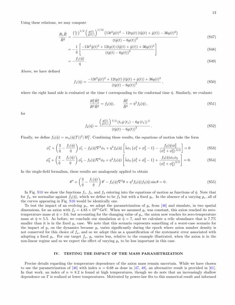
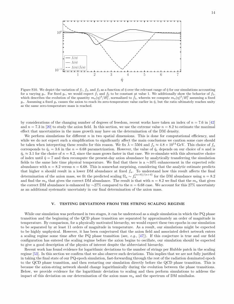
)θ′ − f2(η)∇2θ + η2f2(η)f3(η) sin θ = 0 . (S55)

In Fig. S10 we show the functions f1, f2, and f3 entering into the equations of motion as functions of η. Note thatfor f3, we normalize against f3(η), which we define to be f3 but with a fixed g∗. In the absence of a varying g∗, all ofthe curves appearing in Fig. S10 would be identically one.

To test the impact of an evolving g∗, we adopt the parametrization of g∗ from [46] and simulate, in two spatialdimensions, for an axion with fa = 4.83× 1015 GeV. When we assumed g∗ was constant, this axion reached its zero-temperature mass at η = 3.6, but accounting for the changing value of g∗, the axion now reaches its zero-temperaturemass at η ≈ 5.5. As before, we conclude our simulation at η = 7, and we calculate a relic abundance that is 7.7%smaller than it is in the fixed g∗ case. We note that this scenario represents something of a worst-case scenario forthe impact of g∗ on the dynamics because g∗ varies significantly during the epoch where axion number density isnot conserved for this choice of fa, and so we adopt this as a quantification of the systematic error associated withadopting a fixed g∗. For our target fa, g∗ varies less, relative to the example illustrated, when the axion is in thenon-linear regime and so we expect the effect of varying g∗ to be less important in this case.

IV. TESTING THE IMPACT OF THE MASS PARAMETRIZATION

Precise details regarding the temperature dependence of the axion mass remain uncertain. While we have chosento use the parametrization of [46] with index n = 6.68 as done in [47, 48], an alternative result is provided in [61].In that work, an index of n ≈ 8.2 is found at high temperatures, though we do note that an increasingly shallowdependence on T is realized at lower temperatures. Motivated by power-law fits to this numerical result and informed

14

1 2 3 4 5 6 7

η

10−1

100

f1(η)

f2(η)

f3(η)/f3(η)

Figure S10. We depict the variation of f1, f2, and f3 as a function of η over the relevant range of η for our simulations accountingfor a varying g∗. For fixed g∗, we would expect f1 and f2 to be constant at value 1. We additionally show the behavior of f3,which describes the evolution of the quantity ma(η)2/H2

1 , normalized to f3, wherein we compute ma(η)2/H21 assuming a fixed

g∗. Assuming a fixed g∗ causes the axion to reach its zero-temperature value earlier in η, but the ratio ultimately reaches unityas the same zero-temperature mass is reached.

by considerations of the changing number of degrees of freedom, recent works have taken an index of n = 7.6 in [42]and n = 7.3 in [20] to study the axion field. In this section, we use the extreme value n = 8.2 to estimate the maximaleffect that uncertainties in the mass growth may have on the determination of the DM density.

We perform simulations for different n in two spatial dimensions. This is done for computational efficiency, andwhile we do not expect such a simplification to significantly affect the main conclusions we caution some care shouldbe taken when interpreting these results for this reason. We fix λ = 5504 and fa ≈ 4.8× 1014 GeV. This choice of facorresponds to ηc = 3.6 in the n = 6.68 parametrization. However, the value of ηc depends on our choice of n and isηc ≈ 3.1 for the choice of n = 8.2, since the mass grows faster in that case. We re-simulate with this alternative choiceof index until η = 7 and then recompute the present-day axion abundance by analytically transferring the simulationfields to the same late time physical temperature. We find that there is a ∼10% enhancement in the expected relicabundance with n = 8.2 versus n = 6.68. This is somewhat surprising, considering that the analytic estimate predictsthat higher n should result in a lower DM abundance at fixed fa. To understand how this result affects the final

determination of the axion mass, we fit the predicted scaling Ωa ∼ f (n+6)/(n+4)a for the DM abundance using n = 8.2

and find the ma that gives the correct DM abundance. The result is that with n = 8.2 we find that the ma that givesthe correct DM abundance is enhanced by ∼27% compared to the n = 6.68 case. We account for this 27% uncertaintyas an additional systematic uncertainty in our final determination of the axion mass.

V. TESTING DEVIATIONS FROM THE STRING SCALING REGIME

While our simulation was performed in two stages, it can be understood as a single simulation in which the PQ phasetransition and the beginning of the QCD phase transition are separated by approximately an order of magnitude intemperature. By comparison, for a physically motivated hierarchy, we would expect these two epochs in our simulationto be separated by at least 11 orders of magnitude in temperature. As a result, our simulations might be expectedto be highly unphysical. However, it has been conjectured that the axion field and associated defect network entersa scaling regime some time after the PQ phase transition (see, e.g., [47]). If this conjecture is true and our fieldconfiguration has entered the scaling regime before the axion begins to oscillate, our simulation should be expectedto give a good description of the physics of interest despite the abbreviated hierarchy.

Recent work has found evidence for logarithmic deviations to the number of strings per Hubble patch in the scalingregime [53]. In this section we confirm that we also observe such deviations. This implies that we are not fully justifiedin taking the final state of our PQ-epoch simulation, fast-forwarding through the rest of the radiation dominated epochto the QCD phase transition, and then restarting our simulation directly before the QCD phase transition. This isbecause the axion-string network should change logarithmically during the evolution between the phase transitions.Below, we provide evidence for the logarithmic deviation to scaling and then perform simulations to address theimpact of this deviation on our determination of the axion mass ma and the spectrum of DM minihalos.

15

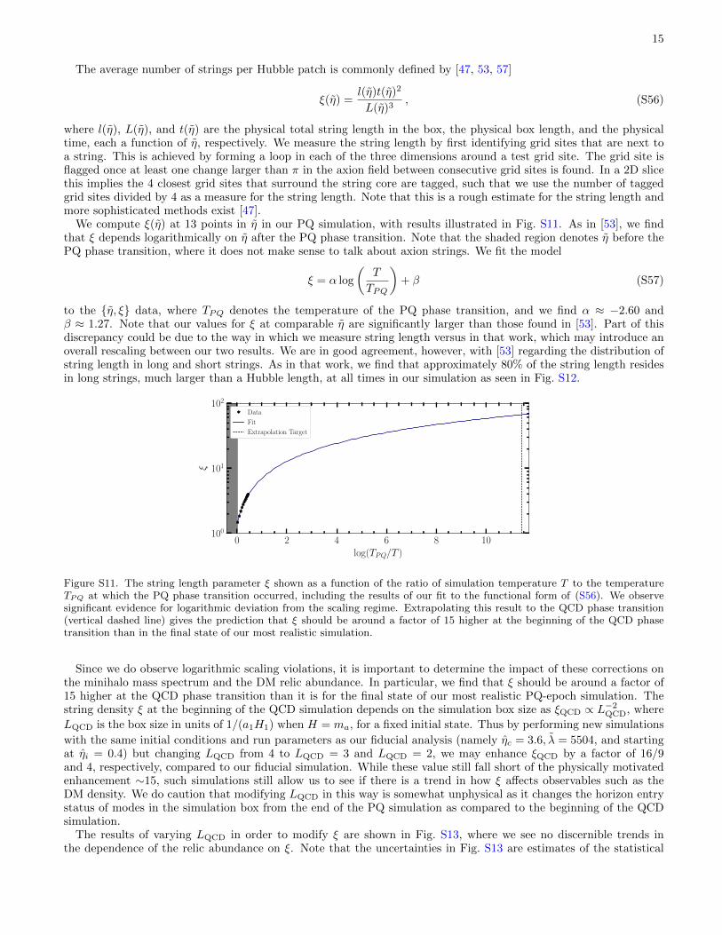
The average number of strings per Hubble patch is commonly defined by [47, 53, 57]

ξ(η) =l(η)t(η)2

L(η)3, (S56)

where l(η), L(η), and t(η) are the physical total string length in the box, the physical box length, and the physicaltime, each a function of η, respectively. We measure the string length by first identifying grid sites that are next toa string. This is achieved by forming a loop in each of the three dimensions around a test grid site. The grid site isflagged once at least one change larger than π in the axion field between consecutive grid sites is found. In a 2D slicethis implies the 4 closest grid sites that surround the string core are tagged, such that we use the number of taggedgrid sites divided by 4 as a measure for the string length. Note that this is a rough estimate for the string length andmore sophisticated methods exist [47].

We compute ξ(η) at 13 points in η in our PQ simulation, with results illustrated in Fig. S11. As in [53], we findthat ξ depends logarithmically on η after the PQ phase transition. Note that the shaded region denotes η before thePQ phase transition, where it does not make sense to talk about axion strings. We fit the model

ξ = α log

(T

TPQ

)+ β (S57)

to the η, ξ data, where TPQ denotes the temperature of the PQ phase transition, and we find α ≈ −2.60 andβ ≈ 1.27. Note that our values for ξ at comparable η are significantly larger than those found in [53]. Part of thisdiscrepancy could be due to the way in which we measure string length versus in that work, which may introduce anoverall rescaling between our two results. We are in good agreement, however, with [53] regarding the distribution ofstring length in long and short strings. As in that work, we find that approximately 80% of the string length residesin long strings, much larger than a Hubble length, at all times in our simulation as seen in Fig. S12.

0 2 4 6 8 10log(TPQ/T )

100

101

102

ξ

Data

Fit

Extrapolation Target

Figure S11. The string length parameter ξ shown as a function of the ratio of simulation temperature T to the temperatureTPQ at which the PQ phase transition occurred, including the results of our fit to the functional form of (S56). We observesignificant evidence for logarithmic deviation from the scaling regime. Extrapolating this result to the QCD phase transition(vertical dashed line) gives the prediction that ξ should be around a factor of 15 higher at the beginning of the QCD phasetransition than in the final state of our most realistic simulation.

Since we do observe logarithmic scaling violations, it is important to determine the impact of these corrections onthe minihalo mass spectrum and the DM relic abundance. In particular, we find that ξ should be around a factor of15 higher at the QCD phase transition than it is for the final state of our most realistic PQ-epoch simulation. Thestring density ξ at the beginning of the QCD simulation depends on the simulation box size as ξQCD ∝ L−2

QCD, where

LQCD is the box size in units of 1/(a1H1) when H = ma, for a fixed initial state. Thus by performing new simulations

with the same initial conditions and run parameters as our fiducial analysis (namely ηc = 3.6, λ = 5504, and startingat ηi = 0.4) but changing LQCD from 4 to LQCD = 3 and LQCD = 2, we may enhance ξQCD by a factor of 16/9and 4, respectively, compared to our fiducial simulation. While these value still fall short of the physically motivatedenhancement ∼15, such simulations still allow us to see if there is a trend in how ξ affects observables such as theDM density. We do caution that modifying LQCD in this way is somewhat unphysical as it changes the horizon entrystatus of modes in the simulation box from the end of the PQ simulation as compared to the beginning of the QCDsimulation.

The results of varying LQCD in order to modify ξ are shown in Fig. S13, where we see no discernible trends inthe dependence of the relic abundance on ξ. Note that the uncertainties in Fig. S13 are estimates of the statistical

16

1.00 1.25 1.50 1.75 2.00 2.25 2.50 2.75TPQ/T

0.80

0.82

0.84

0.86

0.88

0.90

ξ lon

g/ξ

tota

l

Figure S12. The fraction of the string length in super-horizon length strings. Like [53], we find roughly 80% of the string lengthresides within long strings.

4 6 8 10 12 14 16ξQCD

1800

1900

2000

2100

2200

Ωa

LQCD = 4

LQCD = 3

LQCD = 2

Figure S13. The present day axion abundance as a function of the string density parameter ξ at the beginning of the QCDsimulation at ηi = 0.4. Individual data points are labeled by their box length LQCD. The error bars are estimates of thestatistical uncertainties, and no clear trend is visible in the data.

uncertainty. As the box size gets smaller the statistical uncertainty increases. However, we caution that these areestimates only, as we have not run multiple independent simulations for each box size due to computational limitations.It is possible that the true uncertainties at small box sizes are larger than indicated due to the fact that there area small number of e.g. domain walls that form these cases. Still, to be maximally conservative given the availabledatasets, we estimate the difference between the LQCD = 2 and LQCD = 3 values for Ωa as a systematic uncertaintyinduced from the deviation to scaling. However, we cannot be sure that this difference is not a result of statistics or

10−18 10−17 10−16 10−15 10−14 10−13 10−12

M [M]

0.0

0.2

0.4

df/d

logM

LQCD = 4, ηi = 0.4

LQCD = 3, ηi = 0.4

LQCD = 2, ηi = 0.4

LQCD = 3, ηi = 0.3

Figure S14. Differential mass spectrum as a function of the minihalo mass M for different box sizes. Error bands includestatistical errors and the uncertainty on the overall normalisation.

17

from the way in which we artificially mock up initial conditions with higher ξ values. The systematic uncertainty weassign from these tests is 15% correlated between different fa points.

We show in Fig. S14 the impact on the minihalo mass spectrum. Again, all simulations largely agree within theirerror bands (estimated from statistical uncertainties), indicating that an increase in ξ has only a marginal effect onthe late-time axion field. Note that computational resources limit us to just these three additional simulations, andwe leave a more detailed investigation of the dependence of Ωa on ξ to future work.